

1. Introduction
Trade plays a critical role in driving development by facilitating specialization, boosting efficiency, fostering innovation and expanding access to diverse products, among other benefits (Balassa, Reference Balassa1978; Frankel and Romer, Reference Frankel and Romer1999). All these reasons incite countries to participate in trade by adding domestic value to different intermediate and final products and services. The examination of the value-added content of bilateral trade as a measure of trade has become even more necessary nowadays, as the fragmentation of production in many countries is increasing (Antràs and Chor, Reference Antràs and Chor2021). According to the estimation by Johnson and Noguera (Reference Johnson and Noguera2012), approximately two-thirds of global trade can be attributed to the trade in intermediate inputs. The level of domestically generated value added is contingent on diverse characteristics inherent to industries or countries, where the degree of environmental policy stringency (EPS) is a potential factor influencing countries’ participation in bilateral trade (Grossman and Krueger, Reference Grossman and Krueger1991; Porter and van der Linde, Reference Porter and van der Linde1995). Continuously examining the effectiveness and the consequences of environmental policies can yield insights to better shape forthcoming intervention strategies.
Within the literature, policy instruments are divided into two primary categories: market-based and non-market-based (Stavins, Reference Stavins, Mäler and Vincent2003; de Serres et al., Reference de Serres, Murtin and Nicoletti2010; Görlach, Reference Görlach2013). Market-based instruments use changes in market signals to induce behavioural changes; in contrast, non-market-based instruments rely on obligations or non-monetary incentives to influence agent behaviour (Görlach, Reference Görlach2013). These instruments related to environmental regulation may take the form of clauses embedded in non-tariff measures (NTMs) with environmental objectives, environmental provisions within international agreements or negotiations and domestic environmental policies. This paper focuses on the latter. Additionally, the literature addresses the distinct responses of intermediate and final goods and services trade to various factors such as trade costs and market size (Miroudot et al., Reference Miroudot, Lanz and Ragoussis2013). Miroudot et al. (Reference Miroudot, Lanz and Ragoussis2013) argue that trade in intermediates exhibits a relatively high demand elasticity owing to its reduced reliance on consumer preferences and lessened exposure to ‘home bias’. Considering this, in this paper we examine the impact of market and non-market environmental policy instruments on bilateral trade (measured by gross exports and domestic value-added (DVA) in exports) in intermediate and final goods and services at the industry level.
Numerous studies conducted over the years have focused on the complex relationship between stricter environmental standards (including NTMs, environmental provisions in trade agreements or domestic environmental policies) and trade or competitiveness, and the results of these investigations have yielded a diverse range of findings.Footnote 1 Recent empirical literatureFootnote 2 has made notable progress by incorporating trade data expressed in value-added terms, utilizing various types of disaggregated data and employing different estimation methods compared to prior literature. Among these papers, the studies closest to our approach are Koźluk and Timiliotis (Reference Koźluk and Timiliotis2016) and Ederington et al. (Reference Ederington, Paraschiv and Zanardi2022). Koźluk and Timiliotis (Reference Koźluk and Timiliotis2016) estimate a gravity model of bilateral manufacturing exports for 32 countries over 1990–2000, also incorporating DVA exports for selected years. Their main explanatory variable is the EPS gap between countries. Using Poisson Pseudo Maximum Likelihood (PPML), they find no overall effect on manufacturing exports or value added, but show that stricter environmental regulations reduce the competitiveness of high-polluting industries while benefiting low-polluting industries. Ederington et al. (Reference Ederington, Paraschiv and Zanardi2022) examine the effect of differences in international environmental agreements on bilateral manufacturing exports using a gravity model with time-varying country fixed effects. Using data for 63 countries over 1995–2007, they also find negative effects on high-polluting industries and a shift towards low-polluting goods, with stronger long-run effects.
This paper adds three key contributions to the existing literature. Firstly, we empirically estimate a theory-based gravity model, using the exporter-industry-time and importer-industry-time fixed effects as proxies for the Multilateral Resistance Terms (MRTs). Secondly, considering the different tools used by market and non-market instruments, we account for the heterogeneous effects of these instruments on trade, using the latest Organisation for Economic Co-operation and Development (OECD) dataset on EPS. Finally, we analyse gross trade data (for the structural gravity model) as well as trade in value-added terms (for the reduced form model) for intermediate and final goods and services, owing to the growing trade in intermediates and its distinct sensitivity compared to trade in finals. Moreover, we use data from the World Input-Output Database (WIOD) for all 56 industries of the International Standard Industrial Classification Rev.4 (separated into four main sectors: agriculture and fishing; manufacturing; services; and mining, quarrying, water and electricity) in 32 countries during 2000–2014. To the best of our knowledge, this is the first paper to incorporate all of these elements.
The remainder of the paper is organized as follows. Section 2 reviews EPS measures and the theoretical relationship between environmental regulation and trade. Section 3 presents the empirical strategy, data and variables. Section 4 reports the empirical results, including sectoral and manufacturing-level analyses and transmission channels. Section 5 provides robustness checks, and Section 6 concludes.
2. Environmental policy and trade
2.1. Environmental policy instruments and stringency
Based on previous literature, Sorrell et al. (Reference Sorrell, Smith, Betz, Walz, Boemare, Quirion, Sijm, Konidari, Vassos, Haralampopoulos and Pilinis2003) fragment policy design into four elements: instrument, implementation network, target group(s) and outcomes. They define the policy instrument as a law, regulatory tool, initiative, etc., introduced by a governing authority to tackle a specific issue and attain specific goals (Sorrell et al., Reference Sorrell, Smith, Betz, Walz, Boemare, Quirion, Sijm, Konidari, Vassos, Haralampopoulos and Pilinis2003, pp. 14–15). Within the literature, a common classification divides these instruments into two primary categories: market-based and non-market-based (Stavins, Reference Stavins, Mäler and Vincent2003; de Serres et al., Reference de Serres, Murtin and Nicoletti2010; Görlach, Reference Görlach2013). Market-based instruments use changes in market signals (such as prices) to induce behavioural changes; in contrast, non-market-based instruments rely on obligations or non-monetary incentives to encourage or discourage agent behaviour (Görlach, Reference Görlach2013, p. 25).
The stringency of environmental policy is defined as the higher cost of environmentally harmful behaviour or outcomes (Botta and Koźluk, Reference Botta and Koźluk2014). Brunel and Levinson (Reference Brunel and Levinson2013) provide an insightful analysis of the key conceptual hurdles involved in measuring environmental stringency.Footnote 3 Despite the challenges, different indicators measuring EPS have been developed and used in the literature. In their recent work, Galeotti et al. (Reference Galeotti, Salini and Verdolini2020) assess different indicators and group them into four main categories (similar to the five categories of Brunel and Levinson (Reference Brunel and Levinson2013)), specifically, pollution-abatement effort or costs, direct assessments of specific regulations, emission-based indexes,Footnote 4 and composite indicators. More recently, authors have used composite indexes that assess the multidimensionality of environmental regulation.Footnote 5 Considering the drawbacks of the existing environmental stringency indicators and the taxonomy by de Backer and Miroudot (Reference de Backer and Miroudot2013), Botta and Koźluk (Reference Botta and Koźluk2014) constructed a new quantitative policy-based composite index of EPS. They used quantitative and qualitative information to construct an index on market and non-market environmental policy instruments. Kruse et al. (Reference Kruse, Dechezleprêtre, Saffar and Robert2022) updated this index; the updated measure of market and non-market instrument components of environmental policy regulations are shown in Table A1 in Appendix A.Footnote 6
Due to data limitations, the updated EPS index covers climate change and air pollution mitigation policies but excludes other environmental dimensions.Footnote 7 The EPS index is available for 33 countries over 1990–2020 and ranges from 0 to 6, with higher values indicating stricter environmental policies. Market-based instruments include trading schemes and taxes, whereas non-market-based instruments impose emission limits. To our knowledge, the EPS index is the only composite indicator distinguishing between market- and non-market-based instruments while remaining comparable across countries and over time. Given our focus on heterogeneous environmental policy instruments and trade, we use the EPS index (OECD, 2016) and its components as proxies for EPS throughout the analysis.
Figure B1 in Appendix B shows changes in the EPS index and its market and non-market components for OECD and BRIIC (Brazil, Russia, India, Indonesia, and China) countries between 2000 and 2014.Footnote 8 In most countries, standards and emission limits are stricter than pollution pricing instruments and continue to tighten over time, whereas market-based instruments fluctuate more over time. For BRIIC countries (Figure B2 in Appendix B), EPS is generally lower, although China and India have moved towards stricter environmental policies. Figure B1 also shows pronounced increases in non-market-based policy stringency around 2005 and 2012–2013.Footnote 9 These patterns highlight the importance of analysing market- and non-market-based instruments separately, as they follow different dynamics and may generate different incentives for firms.
2.2. Trade
Traditional trade measures, largely based on gross export and import values, have long served as key indicators of trade performance; they remain useful for capturing the scale of cross-border transactions. Given the double-counting issue associated with these measures, alternative analytical frameworks have been developed to disaggregate gross trade flows into components of DVA and double-counted terms. These frameworks can provide insights into the extent to which export values and DVA are directionally aligned and comparable in magnitude. Wang et al. (Reference Wang, Wei and Zhu2013) and Koopman et al. (Reference Koopman, Wang and Wei2014) have presented useful, closely related frameworks for decomposing the sources of value added in gross exports. Wang et al. (Reference Wang, Wei and Zhu2013) group the components of gross exports into four main categories, as illustrated in Figure A1 in Appendix A.Footnote 10 We adopt the decomposing approach followed by these authors as it extends the methodology from a country’s aggregate exports to a bilateral-industry level analysis, which aligns with the focus of this study.
According to this decomposition method, a country’s gross exports contain domestic content (absorbed abroad or returned home), foreign content and double-counted terms. Using the data from the WIODFootnote 11 (Timmer et al., Reference Timmer, Dietzenbacher, Los, Stehrer and De Vries2015) and employing the matrix transformations outlined by Wang et al. (Reference Wang, Wei and Zhu2013), we compute the DVA, foreign value added and double-counted terms in exports, as well as final gross exports and intermediate gross exports, for 2000 and 2014; these calculations are presented in Table B1 in Appendix B. These results further reinforce the notion that a significant portion of trade predominantly involves intermediate goods and services (Johnson and Noguera, Reference Johnson and Noguera2012). A small share of exports is returned home after being exported, while the value of foreign value added and double-counting terms, on average, are more considerable. On average, the DVA in exports has declined from 2000 to 2014, whereas foreign value added and double-counted terms have increased; this can be attributed to production fragmentation in recent years (Antràs and Chor, Reference Antràs and Chor2021). The same pattern holds for gross exports. These statistics indicate a difference between gross exports and exports measured in value-added terms. The difference increases as the level of foreign value added in exports rises (for countries such as Belgium, the Czech Republic, Hungary and Ireland), and vice versa (smaller differences for countries such as Japan, the United States and Brazil); however, these are shares over all industries, and the share for each country’s industry may differ.
In Table B2 in Appendix, we calculated the percentage difference between gross exports and DVA in exports for each industry (averaged across more than 32 countries from 2000 to 2014). On average, industries within the manufacturing sector exhibit the largest differences between gross exports and DVA in exports of intermediate inputs; specifically, in basic metals and non-metal products, coke and refined petroleum products, electrical equipment, and chemicals and chemical products. This can be related to their complex global supply chains (de Backer and Miroudot, Reference de Backer and Miroudot2013).
2.3. Environmental policy and trade – background and hypothesis
The two main hypotheses linking environmental regulation and trade are the Pollution Haven Hypothesis (PHH) and the Porter Hypothesis. The PHH suggests that stringent environmental regulations increase production costs, encouraging firms to relocate pollution-intensive activities to countries with laxer standards (Grossman and Krueger, Reference Grossman and Krueger1991). By contrast, the Porter Hypothesis argues that stringent environmental policies can stimulate innovation and efficiency improvements that enhance firms’ competitiveness (Porter and van der Linde, Reference Porter and van der Linde1995). Policy design plays a central role in shaping the effects of environmental regulation on trade performance through its impact on firms’ production decisions, innovation incentives and productivity dynamics. These effects depend in particular on the distinction between market-based and non-market-based instruments, which generate systematically different optimization environments for firms and therefore distinct channels of transmission to trade outcomes.
Non-market-based instruments operate through direct regulatory constraints, which shift firms’ problem from continuous cost minimization to constraint satisfaction, where the key margin is compliance with exogenously defined requirements. Adjustment is therefore discrete and rule-based, relying on the adoption of existing abatement technologies or incremental process modifications compatible with regulatory thresholds. This tends to generate emission reductions in emission intensity that are achieved in a more ‘stepwise’ and technology-specific manner, and not necessarily present in the short term. Because compliance is evaluated against fixed criteria, firms face limited scope for input substitution or exploration of alternative production pathways. Innovation is thus primarily implementation-oriented, and productivity effects arise mainly through compliance-driven reallocation rather than sustained efficiency improvements (Guo et al., Reference Guo, Fu and Sun2021; Hu et al., Reference Hu, Sun and Dai2021; Lin et al., Reference Lin, Wang and Liu2025). Any innovation response is, moreover, conditional, emerging primarily when standards align with feasible technologies and firms have sufficient absorptive capacity.
By contrast, market-based instruments preserve firms’ optimization problem while introducing a continuous shadow price on emissions. This maintains the full choice set but alters relative prices, embedding environmental regulation within firms’ cost-minimization framework. Firms can continuously trade off abatement and production efficiency through input substitution, process innovation and output adjustment. Because emissions carry a marginal cost rather than a binding constraint, firms face incentives to reduce their overall cost curve, generating cumulative and dynamic innovation under persistent price pressure(Hu et al., Reference Hu, Sun and Dai2021; Fabrizi et al., Reference Fabrizi, Gentile, Guarini and Meliciani2024; Lin et al., Reference Lin, Wang and Liu2025). This mechanism leads to more continuous reductions in emission intensity (mainly in high-polluting industries), as firms optimize along the entire production margin rather than adjusting only at regulatory thresholds. The strength of this mechanism depends on price credibility and policy stability, as uncertainty may weaken intertemporal innovation incentives and shift behaviour towards short-run compliance (Benatti et al., Reference Benatti, Groiss, Kelly and Lopez-Garcia2024).
These differences in adjustment mechanisms imply distinct effects on the firm-level productivity distribution, which is central to heterogeneous-firm models of trade (e.g., Melitz, Reference Melitz2003). Market-based instruments, by inducing continuous cost-reducing innovation, tend to shift and stretch the productivity distribution, making export entry more likely and strengthening export intensity among incumbents. Non-market-based instruments generate more localized and threshold-driven productivity adjustments concentrated around compliance requirements. These adjustments are less likely to translate into persistent productivity gains, thereby limiting both export entry and expansion margins. Taken together, market-based instruments are expected to exert stronger and more persistent effects on trade outcomes than non-market-based instruments.
Before presenting the empirical strategy, we provide graphical evidence to motivate the hypotheses. Given the divergent trends in DVA across intermediate and final exports (Section 2.2), we analyse these variables separately for 2000 and 2014. Figures A2 and A3 in Appendix A present export shares for low-, medium- and high-polluting manufacturing and service sectorsFootnote 12 using data from the WIOD environmental accounts (Corsatea et al., Reference Corsatea, Lindner, Arto, Roman, Rueda-Cantuche, Velazquez Afonso, De Amores and Neuwahl2019) for non-OECD countries, OECD countries with relatively low average EPS values and OECD countries with relatively high average EPS values.Footnote 13 Equivalent graphs using DVA in exports are reported in Figures B2 and B3 in Appendix B.
Figures A2 and A3 in Appendix A show that non-OECD countries and OECD countries with relatively lax environmental policies exhibit higher intermediate export shares in high-polluting industries than in low-polluting sectors. OECD countries with relatively stringent environmental policies exhibit relatively higher final export shares in low-polluting industries. Overall changes between 2000 and 2014 are modest. Non-OECD countries shift towards low-polluting industries, whereas OECD countries exhibit the opposite trend. Manufacturing also appears more environmentally efficient than services, partly due to high emissions in transport services and the downstream nature of the sector. Similar patterns emerge for DVA in exports, although final exports from low-polluting manufacturing industries remain smaller relative to DVA in export shares.
Overall, countries with relatively high EPS values appear to have lower export shares in low-polluting industries. However, these shares decline over time, as do high-polluting export shares in non-OECD countries. This may reflect increasingly stringent environmental policies in major non-OECD countries, particularly China and India. By contrast, several OECD countries using market-based instruments (e.g., Germany, Austria and Greece) exhibit the reverse trend. DVA in export shares show similar patterns. These patterns suggest several hypotheses. First, stricter environmental regulations in countries with traditionally lax standards may shift production away from high-polluting industries or towards cleaner processes. Second, the estimated effects are expected to differ across sectors and between final and intermediate trade, but less between gross and DVA-based exports. The next section outlines the empirical strategy.
3. Empirical strategy and data
We analyse the effects of the EPS gap on international trade measures using a disaggregated structural gravity model. Several authors have derived the disaggregated gravity model from both the supply side (Eaton and Kortum, Reference Eaton and Kortum2002) and the demand side (Anderson and van Wincoop, Reference Anderson and van Wincoop2003). Yotov et al. (Reference Yotov, Piermartini, Monteiro and Larch2016) have shown that in both cases, the disaggregated structural gravity system is given by:
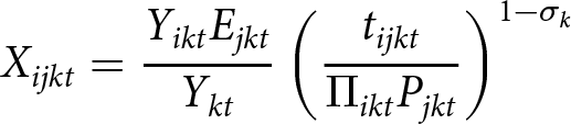 \begin{equation}
X_{ijkt}=\frac{Y_{ikt}E_{jkt}}{Y_{kt}}\left ( \frac{t_{ijkt}}{\Pi_{ikt}P_{jkt}}\right)^{1-\sigma_k}
\end{equation}
\begin{equation}
X_{ijkt}=\frac{Y_{ikt}E_{jkt}}{Y_{kt}}\left ( \frac{t_{ijkt}}{\Pi_{ikt}P_{jkt}}\right)^{1-\sigma_k}
\end{equation}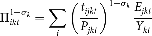 \begin{equation}
\Pi_{ikt} ^{1-\sigma_k}=\sum_{i}^{}\left ( \frac{t_{ijkt}}{P_{jkt}} \right )^{1-\sigma_k }\frac{E_{jkt}}{Y_{kt}}
\end{equation}
\begin{equation}
\Pi_{ikt} ^{1-\sigma_k}=\sum_{i}^{}\left ( \frac{t_{ijkt}}{P_{jkt}} \right )^{1-\sigma_k }\frac{E_{jkt}}{Y_{kt}}
\end{equation}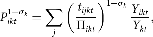 \begin{equation}
P_{ikt} ^{1-\sigma_k}=\sum_{j}^{}\left ( \frac{t_{ijkt}}{\Pi_{ikt}} \right )^{1-\sigma_k}\frac{Y_{ikt}}{Y_{kt}},
\end{equation}
\begin{equation}
P_{ikt} ^{1-\sigma_k}=\sum_{j}^{}\left ( \frac{t_{ijkt}}{\Pi_{ikt}} \right )^{1-\sigma_k}\frac{Y_{ikt}}{Y_{kt}},
\end{equation} where  $X_{ijkt}$ denote the nominal trade flow from exporter $i$ to importer $j$ from industry $k$ at time $t$;
$t$;  $Y_{ikt}$ and $Y_{kt}$ are, respectively, the value of output and the value of global output; $E_{jkt}$ is the level of expenditures; $t_{ijkt}$ denotes bilateral trade costs; $\sigma$ is the elasticity of substitution among different varieties; and $\Pi_{ikt}$ and $P_{jkt}$ are the so-called MRTs. Given the form of the disaggregated structural gravity model in Equation (1), we can log-linearize it and include an additive error term, assuming that this equation holds for each period (Yotov et al., Reference Yotov, Piermartini, Monteiro and Larch2016). The additive form of it looks like the following:
 \begin{equation}
lnX_{ijkt}=lnY_{ikt}+lnE_{jkt}-lnY_{kt}+(1-\sigma_k)\,lnt_{ijkt}-(1-\sigma_k)\,ln\Pi_{ikt}-(1-\sigma_k)\,lnP_{jkt}+\varepsilon_{ijkt}.
\end{equation}
\begin{equation}
lnX_{ijkt}=lnY_{ikt}+lnE_{jkt}-lnY_{kt}+(1-\sigma_k)\,lnt_{ijkt}-(1-\sigma_k)\,ln\Pi_{ikt}-(1-\sigma_k)\,lnP_{jkt}+\varepsilon_{ijkt}.
\end{equation} Anderson and van Wincoop (Reference Anderson and van Wincoop2003) refer to the  $\Pi_{ikt}$ as the outward multilateral resistances and $P_{jkt}$ as inward multilateral resistances, which measure, respectively, the ease that exporter $i$ or importer $j$ have to access markets. The MRTs are not directly observable, and several approaches are reported in the literature to address this issue, including nonlinear programming, estimation of the ratio-based gravity model, construction of ‘remoteness indexes’ and the usage of fixed effects. Using fixed effects is the preferred method for most empirical applications (Head et al., Reference Head, Mayer and Ries2010). However, failing to use the proper form of these fixed effects has been shown to affect coefficient magnitudes and significance (Borchert et al., Reference Borchert, Larch, Shikher and Yotov2022). Yotov et al. (Reference Yotov, Piermartini, Monteiro and Larch2016) and Borchert et al. (Reference Borchert, Larch, Shikher and Yotov2022) suggest that the appropriate fixed effects are exporter-industry-time and importer-industry-time fixed effects when estimating the structural gravity model disaggregated at the industry level.
Moreover, Borchert et al. (Reference Borchert, Larch, Shikher and Yotov2022) recommend that the structural gravity model should be estimated including country-pair fixed effects to account for all time-invariant country-pair variables and to lessen the endogeneity concerns. On the contrary, Aichele and Felbermayr (Reference Aichele and Felbermayr2015) use country-pair-industry fixed effects to capture all unobserved country-pair fixed effects at the industry level (these fixed effects absorb the country-pair factors also). Hence, we use country-pair fixed effects to control for unobserved country-pair and country-pair-industry factors. Also, the sectoral bilateral costs are proxied in the structural gravity model, mostly by using observable variables. We utilize the standard covariates used in empirical literature as determinants of trade frictions between countries, including here the distance between countries, the presence of contiguous borders, the official language or colonial ties, the existence of any regional trade agreements (RTAs), as well as any policy-related variable.Footnote 14 Except for the last two variables, all other variables are absorbed by the fixed effects discussed above. In addition, Borchert et al. (Reference Borchert, Larch, Shikher and Yotov2022) propose using the PPML estimator to account for potential heteroscedasticity and zero trade data flows. Fally (Reference Fally2015) argues that estimating the gravity model with fixed effects using other estimators different from PPML is not consistent with the theoretical gravity framework developed by Anderson and van Wincoop (Reference Anderson and van Wincoop2003).
We employ all the above-mentioned elements and estimate the ‘comprehensive econometric version of the structural gravity model’ (Yotov et al., Reference Yotov, Piermartini, Monteiro and Larch2016). Some of the variables ( $Y^k_{i,t}$, $Y^k_{t}$, $E^k_{j,t}$) in Equation (1) are absorbed by fixed effects, leading to the following form:
 \begin{equation}
X_{ijkt}=exp[\beta_{1}lnt_{ijkt}+\phi_{ikt}+\phi_{jkt} +\phi_{ijk}] \times \varepsilon_{ijkt},
\end{equation}
\begin{equation}
X_{ijkt}=exp[\beta_{1}lnt_{ijkt}+\phi_{ikt}+\phi_{jkt} +\phi_{ijk}] \times \varepsilon_{ijkt},
\end{equation}where  $\phi_{ikt}$ and $\phi_{jkt}$ are, respectively, exporter-industry-time and importer-industry-time fixed effects, $\phi_{ijk}$ are the country-pair-industry fixed effects and $\varepsilon_{ijkt}$ are the regression residuals. As noted above, all other proxies for trade frictions are absorbed by the fixed effects in Equation (5), except for RTAs and policy-related variables (here, environmental policy). We aim to test how differences in environmental policies, and in particular, changes in these differences between countries, affect trade between them. We, therefore, use the difference between the exporter’s EPS and the importer’s EPS as a measure of the difference in the EPS between the two countries:Footnote 15
 \begin{equation}
EPSgap_{ijt}=EPS_{it}-EPS_{jt}.
\end{equation}
\begin{equation}
EPSgap_{ijt}=EPS_{it}-EPS_{jt}.
\end{equation}Including exporter–industry–time and importer–industry–time fixed effects also absorb the effects of this difference due to linearity; to address this, we follow the approach employed by Ederington et al. (Reference Ederington, Paraschiv and Zanardi2022), using a non-linearFootnote 16 measure of relative environmental stringency between two countries:
 \begin{equation}
(non-linear)\,EPSgap_{ijt}={(EPS^2_{it}-EPS^2_{jt})}\,/\,{(EPS_{it}+1)\,(EPS_{jt}+1)}.
\end{equation}
\begin{equation}
(non-linear)\,EPSgap_{ijt}={(EPS^2_{it}-EPS^2_{jt})}\,/\,{(EPS_{it}+1)\,(EPS_{jt}+1)}.
\end{equation} One shortcoming of using Equations (6) or (7) as measures of environmental stringency difference is that we cannot distinguish if the changes in 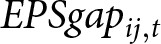 $EPSgap_{ij,t}$ are due to changes in exporters’ EPS index, importers’ EPS index or both. More specifically, an increase in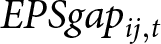 $EPSgap_{ij,t}$ implies stricter environmental regulation by the exporting country or more lax environmental regulation by the importing country, or both; in either case, countries increase ‘divergence’ in the stringency of environmental policies. Our main dependent variables are gross exports and DVA in exports for intermediate and final goods and services. Using gross exports is consistent with the structural gravity model, whereas DVA in exports lacks theoretical grounding and resembles reduced-form estimation. For these variables, we employ the matrix transformation by Wang et al. (Reference Wang, Wei and Zhu2013) using the World Input-Output Tables (WIOTs) for 56 industries published by the WIOD.Footnote 17 Consequently, the final dataset comprises 56 industries across 32 countries for 2000–2014.
To account for the differential effects of changes in EPS gaps on exports across industries by pollution intensity, we introduce an interaction term between the EPS difference and pollution intensity for each industry. Different authors (Levinson, Reference Levinson2009; Shapiro and Walker, Reference Shapiro and Walker2018) decompose the change in a country’s emissions due to changes in production scale, production composition and production techniques (changes in pollution intensity). Changes in environmental regulations may affect production techniques. Because we are interested in production and scale effects (i.e., competitiveness effects), we hold the technique effect constant by keeping emission intensity constant. To do so, we follow the approach by Ederington et al. (Reference Ederington, Paraschiv and Zanardi2022), we calculate sectoral CO2 emissions intensity (CO2 emissions per unit of output) as industry averages over all countries in our dataset during 2000–2014, and we interact it with the EPS difference (a similar strategy is followed by Koźluk and Timiliotis (Reference Koźluk and Timiliotis2016)). We use data from the WIOD environmental accounts (Corsatea et al., Reference Corsatea, Lindner, Arto, Roman, Rueda-Cantuche, Velazquez Afonso, De Amores and Neuwahl2019). Based on WIOT sectors and countries, they provide data on CO2 and energy use; for the main part of our analysis, we use CO2 data (while using energy data for robustness checks). Given that the non-linear EPS gap values differ from the original EPS difference (although highly correlated), we should be cautious in interpreting the coefficient’s magnitude; therefore, the focus of the empirical results should be on the sign and significance. As a consequence, we use the industry CO2 emissions intensity and compute different pollution intensity dummy variables (PIs); the dummy variables are assigned a value of zero when the industry CO2 emissions intensity value (average over all countries and years) is less than the 50th or 75th percentile cutoffs of the intensity of CO2 emissions of all industries.Footnote 18 Consequently, interpreting the interaction term is more complex, as the coefficient on the non-linear EPS gap index lacks a direct interpretation.
As a result of all the aforementioned aspects, the basic specifications that we estimate using the PPML estimator are the following:
 \begin{equation}
X_{ijkt} = exp[\beta_{1}EPSgap_{ijt}+\beta_{2}EPSgap_{ijt}*PI_k+\beta_{3}RTA_{ijt}+\phi_{ikt}+\phi_{jkt} +\phi_{ijk}] \times \varepsilon_{ijkt},
\end{equation}
\begin{equation}
X_{ijkt} = exp[\beta_{1}EPSgap_{ijt}+\beta_{2}EPSgap_{ijt}*PI_k+\beta_{3}RTA_{ijt}+\phi_{ikt}+\phi_{jkt} +\phi_{ijk}] \times \varepsilon_{ijkt},
\end{equation} \begin{equation}
\begin{split}
X_{ijkt} & = exp[\beta_{1}MKTgap_{ijt}+ \beta_{2}NMKTgap_{ijt}+\beta_{3}MKTgap_{ijt}*PI_k+ \\
& \beta_{4}NMKTgap_{ijt}*PI_k+\beta_{5}RTA_{ijt}+\phi_{ikt}+\phi_{jkt} +\phi_{ijk}] \times \varepsilon_{ijkt},
\end{split}
\end{equation}
\begin{equation}
\begin{split}
X_{ijkt} & = exp[\beta_{1}MKTgap_{ijt}+ \beta_{2}NMKTgap_{ijt}+\beta_{3}MKTgap_{ijt}*PI_k+ \\
& \beta_{4}NMKTgap_{ijt}*PI_k+\beta_{5}RTA_{ijt}+\phi_{ikt}+\phi_{jkt} +\phi_{ijk}] \times \varepsilon_{ijkt},
\end{split}
\end{equation} where 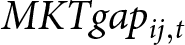 $MKTgap_{ij,t}$ and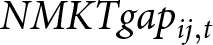 $NMKTgap_{ij,t}$ are the market and non-market instrument differences, respectively. According to Balassa (Reference Balassa1961), RTAs can be classified into five levels of integration: preferential trading arrangement, free trade area, customs union, common market and economic union. Based on this concept, in our analysis,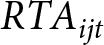 $RTA_{ijt}$ is a categorical variable from 0 to 6 for each level of economic integration (the base category is ‘no-agreement’). The main variables of interest are the non-linear EPS and its interaction with average industry pollution intensity. In Equation (8), $\beta_{1}$ captures the average effect of the EPS difference when the dummy variable of average industry pollution intensity is zero (low-polluting industries), while $\beta_{2}$ captures the effect of changes in EPS gaps for high-polluting compared to low-polluting industries. The coefficients of the variables of interest in Equation (9) can be interpreted using the same intuition.
4. Results
4.1. Baseline results
The estimated results of Equation (8) are reported in Table A3 in Appendix A. This table reveals that there is almost no significant effect of the EPS gap on the export level (measured as gross exports and DVA in exports). The environmental policy gap is weakly significant for final gross exports and DVA in exports; however, given the size of our sample, this significance is not informative for firm conclusions. According to the RTAs, being part of a customs union positively affects trade. The insignificance of other RTA components can be attributed to the relatively large trade flows between countries in our dataset, which do not necessarily exhibit high levels of integration (e.g., several European countries with BRIIC countries).
Table A4 in Appendix A presents the effects of market and non-market environmental policy gaps across countries on gross exports and DVA in exports for intermediate and final goods and services. For the RTA categories,Footnote 19 from here on, we will include only the variables with significant coefficients. When estimating Equation (9) with market- and non-market-based EPS gaps, rather than the EPS gap alone, it is evident that market-environment policy instruments are highly significant and negatively affect intermediate trade (exports and DVA in exports, though for the gross exports the coefficients are relatively higher) for high-polluting industries relative to low-polluting industries. The increase of country differences in these instruments has a positive effect on trade in low-polluting industries, as the coefficient in the market gap variable is positive and highly significant.Footnote 20 Disparities in non-market-based instruments have no significant effect on bilateral trade, a result that may also be influenced by the fact that these instruments vary little over time.
These results, at first glance, seem to confirm the existence of the PHH for trade in intermediates; the stricter the environmental regulations of the exporting country become in comparison to others (or the laxer the environmental policies of the importing country, or both), the more countries export from less-polluting industries while reducing production in high-polluting sectors. However, these patterns may reflect mechanisms beyond the PHH. Stricter environmental regulations may induce innovation and efficiency gains, consistent with the Porter hypothesis, allowing cleaner industries to expand without relocating pollution-intensive production to countries with laxer regulations. These innovation effects may emerge in both low- and high-emission industries, particularly in the long run and alongside innovation in trading partners. Countries may also substitute exports with domestic production and use of pollution-intensive goods. These mechanisms are explored further in Section 4.3.
4.2. Sector level baseline results
In this section, we estimate Equations (8) and (9) for four main sectors: agriculture and fishing; manufacturing; services; and mining, quarrying, water and electricity. The results when using the general EPS index are shown in Tables B4 and B5 in Appendix B, while the results for market and non-market instruments gaps are presented in Tables A5 and A6 in Appendix A.Footnote 21
Consistent with Table A3 in Appendix A, Tables B4 and B5 in Appendix B show no significant effect of environmental regulation differences on bilateral exports in agriculture and fishing, manufacturing or mining, quarrying, water and electricity. For services, Table B5 in Appendix B shows that greater environmental policy divergence increases intermediate exports in low-polluting industries, whereas the opposite pattern emerges for high-polluting industries in final exports. This may reflect that some industries located near the final stages of value chains are relatively pollution-intensive (i.e., transport, postal activities, warehousing and support activities for transportation) (see Table B3 in Appendix B). Moreover, economic integration becomes particularly important for trade in final goods and services, especially in services, agriculture and fishing. These results suggest that countries within common markets or economic unions (e.g., the European Union) trade more intensively in these sectors than in manufacturing or mining and quarrying. This likely reflects the greater geographical dependence of these sectors, whereas manufacturing trade is shaped more by complex supply chains.
In Tables A5 and A6 in Appendix A, we present the results for the market- and non-market-based instrument gaps across the four sectors. Table A5 in Appendix A reports the results for agriculture and fishing, and manufacturing, while Table A6 presents the findings for mining, quarrying, water and electricity and services. Table A5 shows that differences in non-market-based instruments affect final trade (gross exports and DVA in exports) in the agriculture sector, while having no significant effect on manufacturing. By contrast, increases in market-based environmental policy gaps negatively affect bilateral exports (gross exports and DVA in exports) in high-polluting manufacturing industries. Pollution charges and trading schemes are more likely to affect manufacturing firms than agriculture and fishing activities, which generate relatively lower CO2 emissions that are more difficult to monitor and are less exposed to pollution charges.
Turning to Table A6 in Appendix A, we find no significant effect of either market- or non-market-based EPS differences on bilateral exports in the mining, quarrying, water and electricity sector. This supports the argument that these are relatively non-‘footloose’ industries; their high capital intensity limits the ability to relocate production in response to environmental regulations (Ederington et al., Reference Ederington, Levinson and Minier2005). In addition, resource location is likely more important for mining and quarrying activities than regulatory differences across countries. In the service sector, the effect is positive and statistically significant at the 5 per cent level for low-polluting industries when considering intermediate gross exports, although the significance is weaker for DVA in exports of intermediate services. Trade in high-polluting service industries is not negatively affected by changes in market- or non-market-based environmental instrument gaps. Instead, these changes appear to benefit low-polluting service industries, potentially reflecting a ‘first-mover’ advantage for industries already operating with lower pollution levels (Koźluk and Timiliotis, Reference Koźluk and Timiliotis2016).
Table B6 in Appendix B reports results using the 50th-percentile pollution-intensity threshold in the manufacturing and services sectors. The results for services remain broadly consistent with those in Table A6, whereas the estimated effects for manufacturing lose statistical significance relative to Table A5, suggesting that the results are more pronounced when comparing the most polluting industries with all others. As in Tables B4 and B5 in Appendix B, economic integration is particularly important for agriculture and fishing, as well as services. Differences between gross exports and DVA in exports appear to matter mainly for specific industries and country-pair relationships rather than on average, as the results remain broadly similar across both measures, consistent with the correlation coefficients reported in Table A2 in Appendix A.
4.3. Detailed manufacturing sector results
As observed in the previous section, the increase in the gap between non-market-based environmental instruments and other instruments reduces exports from high-polluting manufacturing industries. This negative coefficient is not consistently observed in other sectors; for agriculture, mining, quarrying, water and electricity, the interaction term cannot be estimated due to the limited number of industries within these broader categories. Considering this and the manufacturing sector’s significant contribution to industrial pollution, a more detailed analysis is conducted for this sector. We assess whether the effects observed in Table A5 in Appendix A are attributable to specific bilateral trade relationships. In addition, we explore potential transmission channels.
Given that our dataset includes both OECD and non-OECD countries,Footnote 22 with the latter generally characterized by more lenient environmental regulations, we regress Equation (9) separately for trade flows among four country pairings: non-OECD to non-OECD, non-OECD to OECD, OECD to non-OECD and OECD to OECD. This allows us to determine whether the negative coefficients observed in Table A5 in Appendix A are attributable to particular trade relationships. The detailed results of these regressions are presented in Tables A7 and A8 in Appendix A.Footnote 23
Tables A7 and A8 show that market-based environmental stringency gaps affect trade asymmetrically across country pairs. A widening market-based gap (stricter environmental instruments in origin countries, weaker stringency in destination countries, or both) significantly reduces exports from OECD to non-OECD countries. This pattern suggests that market-based instruments primarily operate through a cost-competitiveness channel, increasing trade frictions for pollution-intensive production; these effects largely drive the aggregate results reported in Table A5 in Appendix A. Within non-OECD country pairs, larger market-based stringency gaps also act as barriers to trade, particularly for final goods that require full compliance with domestic regulations. By contrast, no significant effects are found for exports from non-OECD countries to OECD countries or for trade among OECD countries. By contrast, non-market-based environmental stringency gaps exhibit no significant aggregate effect but substantial bilateral heterogeneity. In particular, wider non-market-based gaps reduce final exports in high-pollution-intensity industries among non-OECD countries, whereas they have no significant effect on exports from non-OECD to OECD countries. Moreover, non-OECD countries increase intermediate exports from low-polluting industries to OECD destinations, which are typically less exposed to final-goods regulatory requirements. Among OECD countries, non-market-based stringency gaps are associated with increases in both final exports from low-polluting industries and intermediate exports from high-polluting industries. These opposing effects explain the non-significant impact on overall manufacturing exports shown in Table A5 in Appendix A.
Taken together, these results highlight important differences across environmental policy instruments and trading partners’ institutional characteristics. Trade with non-OECD countries appears more sensitive to divergence in both market- and non-market-based instruments, particularly the latter. This may reflect that, in countries with weaker regulatory and enforcement capacity, divergence in non-market-based instruments generates compliance costs that are harder to absorb, especially for pollution-intensive final goods. By contrast, exports to OECD countries are generally less adversely affected and often positively associated with greater environmental policy divergence. The expansion of low-polluting final goods exports may reflect a gradual shift towards cleaner production structures, whereas the increase in pollution-intensive intermediate trade within OECD countries more likely reflects technological upgrading or production reorganization rather than a standard pollution haven mechanism. The next section examines these transmission channels in greater detail.
Transmission channels
As discussed in Section 2.3, market-based and non-market-based instruments differ in their adjustment processes. These differences are expected to translate into distinct patterns of efficiency improvement and industrial technology, with implications for international competitiveness.
Emission intensity: A central goal of environmental policy is to reduce overall emissions, which can be achieved by improving emissions intensity through cleaner production processes (Sorrell et al., Reference Sorrell, Smith, Betz, Walz, Boemare, Quirion, Sijm, Konidari, Vassos, Haralampopoulos and Pilinis2003). Emission intensity reductions under non-market-based instruments are more likely to reflect compliance with prescribed standards and are more likely ‘stepwise’, whereas reductions under market-based instruments are more likely continuous and closely linked to cost-minimizing adjustments in production decisions.
Industrial technology: Environmental policy may also shape industrial upgrading by affecting incentives for adopting more advanced production technologies. While market-based instruments are more likely to induce continuous innovation through flexible adjustment margins, non-market-based instruments may also generate upgrading effects when standards align with feasible technologies and firms possess sufficient absorptive capacity. To proxy this, we follow Wang and Ramsey (Reference Wang and Ramsey2024) and construct a measure based on the interaction between revealed comparative advantage (RCA) and labour productivity as follows:
 \begin{equation}
\text{IT}_{k,c} = \frac{\text{x}_{k,c} / \text{X}_c}{\sum_k \text{X}_{k,c} / \sum_c \text{X}_c} \, \text{LP}_{k,c}
= \text{RCA}_{k,c} \, \text{LP}_{k,c},
\end{equation}
\begin{equation}
\text{IT}_{k,c} = \frac{\text{x}_{k,c} / \text{X}_c}{\sum_k \text{X}_{k,c} / \sum_c \text{X}_c} \, \text{LP}_{k,c}
= \text{RCA}_{k,c} \, \text{LP}_{k,c},
\end{equation}where  $k$ denotes the industry, $c$ denotes the country, $X$ are exports and $\text{LP}$ is labour productivity measured as industrial hours worked per unit of value added. As in Wang and Ramsey (Reference Wang and Ramsey2024), rather than using export levels, we use the value added in exports, i.e., the actual value produced in a country and consumed elsewhere.
We examine two transmission channels: first, the impact of market- and non-market environmental instruments on CO2 emissions intensity; and second, their effect on industrial technology. Both channels are estimated using a fixed-effects model at the country–sector level,Footnote 24
 \begin{equation}
\text{CO2Int}_{ckt} = \beta_1 \text{CO2Int}_{c k,t-1} + \,\beta_2 \text{MKT}_{c,t-1} + \,\beta_3 \text{NMKT}_{c,t-1} + \mu_c + \,\lambda_k + \gamma_t + \,\varepsilon_{ckt},
\end{equation}
\begin{equation}
\text{CO2Int}_{ckt} = \beta_1 \text{CO2Int}_{c k,t-1} + \,\beta_2 \text{MKT}_{c,t-1} + \,\beta_3 \text{NMKT}_{c,t-1} + \mu_c + \,\lambda_k + \gamma_t + \,\varepsilon_{ckt},
\end{equation} \begin{equation}
\quad\quad\text{IT}_{ckt} = \beta_1 \text{IT}_{c k,t-1} + \beta_2 \text{MKT}_{c,t-1} + \beta_3 \text{NMKT}_{c,t-1} + \mu_c + \lambda_k + \gamma_t + \varepsilon_{ckt},
\end{equation}
\begin{equation}
\quad\quad\text{IT}_{ckt} = \beta_1 \text{IT}_{c k,t-1} + \beta_2 \text{MKT}_{c,t-1} + \beta_3 \text{NMKT}_{c,t-1} + \mu_c + \lambda_k + \gamma_t + \varepsilon_{ckt},
\end{equation} where  $\mu_c$, $\lambda_k$ and $\gamma_t$ represent country, sector and year fixed effects, respectively. The results, which are presented in Table A9 in Appendix A, indicate that, in non-OECD countries, market-based regulations significantly reduce emission intensity and promote industrial technology upgrading in high-polluting industries. This may help explain why the interaction term for high-polluting industries in Table A7 in Appendix A is insignificant for exports to both OECD and non-OECD destinations. Among OECD countries, non-market-based instruments significantly affect industrial technology in both low- and high-polluting industries, with larger effects in the latter. These findings are consistent with the increase in low-polluting industries reported in Table A8 in Appendix A for the non-market-based instrument gap in columns (6) and (8), suggesting that these effects could be driven by technological changes in these sectors. Moreover, the significant interaction terms in columns (5) and (7) of Table A8 for OECD countries may also reflect an increase in export level due to technological improvements.Footnote 25
As shown in the results section, the manufacturing sector largely drives the decline in exports from high-polluting industries and the expansion of exports from low-polluting industries as gaps in market-based environmental regulations widen. These patterns are mainly driven by OECD–non-OECD trade, with exports declining in high-polluting industries and increasing in low-polluting industries as market-based regulatory divergence rises. The absence of significant effects on emission intensity and industrial technology suggests limited technological adjustment, helping explain the negative export response reported in Table A8 in Appendix A. Consistent with this interpretation, Table B14 in Appendix B shows that the share of high-polluting industries in OECD manufacturing value added declined between 2000 and 2014, while the share of low-polluting industries increased. By contrast, non-OECD countries experienced growth in value added in both low- and high-polluting industries, with no clear evidence of export contraction in pollution-intensive sectors. This is consistent with the positive association between market-based instruments, emission intensity and industrial technology.
By contrast, non-market-based instruments are associated with export expansion in low-polluting industries across both OECD and non-OECD countries. This pattern is reflected in Table B14 in Appendix B, which shows rising value added in low-polluting industries across both country groups, alongside higher exports reported in Tables A7 and A8 in Appendix A. At the same time, greater divergence in non-market-based instruments is associated with higher levels of industrial technology in high-polluting industries within OECD countries and increased intermediate exports to other OECD economies, despite a decline in these industries’ overall share of manufacturing value added between 2000 and 2014. Taken together, these findings suggest that higher exports reflect technological upgrading or specialization within OECD value chains, while declining value-added shares indicate a broader shift towards less pollution-intensive manufacturing.
5. Robustness analysis
5.1. Endogeneity concerns
A central concern in estimating the effects of environmental regulations on trade is endogeneity. This may arise from simultaneity, as governments can adjust environmental policy in response to trade competitiveness, potentially leading to more lenient regulation in export-oriented sectors. In addition, unobserved determinants of trade outcomes may be correlated with environmental stringency, generating omitted variable bias. To address the latter, we include country-pair-industry fixed effects, which absorb time-invariant unobserved heterogeneity at this level of aggregation (Aichele and Felbermayr, Reference Aichele and Felbermayr2015; Yotov et al., Reference Yotov, Piermartini, Monteiro and Larch2016; Borchert et al., Reference Borchert, Larch, Shikher and Yotov2022). Regarding simultaneity, we exploit variation in bilateral differences in environmental policy. Since countries engage in multiple trade relationships across sectors, bilateral industry-level trade flows are unlikely to be a primary determinant of national environmental policy choices. Moreover, we use country-level aggregates of environmental stringency, reducing the influence of industry-specific policy variation potentially driven by trade outcomes. Given that the dependent variable is measured at the country-industry level, this aggregation further limits reverse causality concerns.
A common approach in the literature is to use lagged differences of environmental instruments as explanatory variables, which helps mitigate concerns about contemporaneous reverse causality. This reflects the fact that environmental regulations typically affect production costs and trade flows with a delay due to implementation lags, adjustment costs and pre-existing contractual relationships (Sato and Dechezleprêtre, Reference Sato and Dechezleprêtre2015, Koźluk and Timiliotis, Reference Koźluk and Timiliotis2016). Accordingly, we re-estimate Equations (8) and (9) using first lags of the EPS, market-based and non-market-based instrument gaps between countries; the results are shown in Table B7 in Appendix B. The sign and significance of most interaction terms remain unchanged for market-based instruments. The positive effect of market-based EPS differences largely disappears after the first year, whereas the negative effect on final export competitiveness becomes evident with a one-year lag.
A further concern relates to policy interdependence across countries. A large body of evidence shows that domestic factors are the main determinants of EPS (Athari, Reference Athari2024), although international spillovers and policy diffusion – particularly within economically integrated regions – also play a role in shaping policy convergence (Linsenmeier et al., Reference Linsenmeier, Mohommad and Schwerhoff2023; Cadoret and Padovano, Reference Cadoret and Padovano2024; Döme, Reference Döme2024). Such diffusion is typically gradual and depends on institutional capacity, economic integration and domestic absorptive capacity, thereby reducing cross-country variation. Nevertheless, these processes are unlikely to generate strong contemporaneous bilateral feedback at the industry level.
To further assess this concern, we construct a trade-weighted measure of foreign EPS capturing exposure to trading partners’ regulatory environments. This variable proxies for diffusion operating through trade linkages. However, in our empirical specification, it is absorbed by country-industry-time fixed effects, implying that time-varying exposure to foreign regulations at that level of aggregation is already controlled for in the baseline model. While this mitigates concerns about omitted variable bias from contemporaneous diffusion, it does not fully eliminate slower-moving or network-based diffusion channels not captured by the fixed-effects structure. Although policy diffusion may contribute to longer-run convergence in policy stringency and attenuate coefficients overall, it is unlikely to bias the estimated differential effects between market-based and non-market-based instruments, as importer-industry-time fixed effects absorb contemporaneous exposure to foreign regulatory environments.
Finally, we complement the baseline estimates using the system Generalized Method of Moments estimator of Blundell and Bond (Reference Blundell and Bond1998), with Windmeijer-corrected standard errors (Roodman, Reference Roodman2009). In this setting, we treat environmental instrument gaps (and their interactions) as endogenous, whereas the dependent variables (intermediate exports and DVA in exports) are treated as predetermined. Time dummies are assumed to be strictly exogenous. The results are reported in Table B8 in Appendix B.Footnote 26 The results indicate that the effect of market-based instruments remains robust: the market-based instrument gap retains a positive and statistically significant coefficient, whereas in high-polluting industries a larger gap is associated with a negative and statistically significant effect on intermediate exports. In contrast, the coefficient on non-market-based instruments remains insignificant, consistent with the results reported in Table A4 in Appendix A.
5.2. Control variables
Table A4 in Appendix A shows no statistically significant effect of the gap in non-market-based environmental regulations on bilateral trade. As discussed in Section 4.1, this result may reflect the non-cost-related nature of these instruments and their limited time variation across countries (see Figure B1 in Appendix B). To further investigate this result, and given the close relationship between regulation and enforcement, we re-estimate Equation (9) by interacting the gaps in market- and non-market-based regulations with institutional quality, proxied by the World Bank’s Regulatory Quality Indicator (Kaufmann and Kraay, Reference Kaufmann and Kraay2024).Footnote 27 Moreover, we estimate Equation (9) for 2005 and 2013, during which non-market-based regulations changed more substantially across countries, as well as for 2004–2005, when the Kyoto Protocol entered into force.Footnote 28 Results are reported in Table B9 in Appendix B.Footnote 29 Overall, the main coefficients of Equation (9) remain unchanged. Columns (1)–(4) show that the effect of non-market regulatory gaps on exports from low-polluting industries becomes significant when the destination country has higher institutional quality, suggesting that regulatory differences become more trade-relevant when destination countries have stronger institutions. Furthermore, results for selected years are shown in columns (5)–(8) and indicate that larger non-market-based regulatory gaps are associated with higher bilateral exports of low-polluting goods – both intermediate and final – across low- and high-polluting industries, suggesting a restructuring towards low-polluting industries. The coefficient on the non-market-based gap retains the same sign and significance for 2004–2005.Footnote 30
Although industry rankings may vary across pollutant categories, industries with high pollution levels in one category also tend to be highly polluting in others (Mani and Wheeler, Reference Mani and Wheeler1998; Broner et al., Reference Broner, Bustos and Carvalho2012; Ederington et al., Reference Ederington, Paraschiv and Zanardi2022). This pattern is particularly evident in large industry samples such as ours, supporting the use of CO2 emissions to identify high-polluting industries. This is especially relevant because our pollution-intensity measure is defined as a binary indicator. Nonetheless, we assess the robustness of our results using industry-level data on gross energy use and gross energy use related to CO2 emissions from the WIOD environmental accounts. The results presented in Table B10 in Appendix B show that the coefficients of the interaction terms retain the same signs and significance levels as those reported in Tables A3 and A4. Estimating Equations (8) and (9) using gross energy use related to CO2 emissions yields similar results. Detailed tables are available upon request.
In the literature, authors make different choices regarding the fixed effects used in gravity model estimation. While Borchert et al. (Reference Borchert, Larch, Shikher and Yotov2022) suggest the use of country-industry-time and country-pair fixed effects, Aichele and Felbermayr (Reference Aichele and Felbermayr2015) and Ederington et al. (Reference Ederington, Paraschiv and Zanardi2022) employ country-time, industry-time and country-pair-industry-time fixed effects. We follow the approach proposed by Borchert et al. (Reference Borchert, Larch, Shikher and Yotov2022) and Yotov et al. (Reference Yotov, Piermartini, Monteiro and Larch2016), which effectively addresses MRTs.Footnote 31 To assess the sensitivity of our results to alternative fixed-effects structures, we re-estimate the main regressions following the approach of Aichele and Felbermayr (Reference Aichele and Felbermayr2015) and Ederington et al. (Reference Ederington, Paraschiv and Zanardi2022). The results, reported in Table B11 in Appendix B, indicate a negative and significant effect of market-based EPS differences on exports of final goods and services rather than intermediate inputs. However, country-time fixed effects address MRTs differently from the framework proposed by Yotov et al. (Reference Yotov, Piermartini, Monteiro and Larch2016). Overall, the choice of fixed effects can influence both the sign and significance of estimated coefficients, highlighting the importance of appropriate fixed-effects specification in gravity models.Footnote 32
5.3. Sensitivity analysis
In our first sensitivity analysis, we examine the potential influence of countries with unique development trajectories that may disproportionately affect trade outcomes. To investigate this, we re-estimate Equations (8) and (9) for EPS, as well as the differences between its market and non-market components, excluding China from the dataset. The results are presented in Table B12 in Appendix B. We find that the market-based variable maintains similar signs and significance levels to those reported in Section 4 (see also Tables A3 and A4 in Appendix A). Non-market-based instruments are significant for final exports in low-polluting industries, indicating that changes in this instrument gap confer a comparative advantage on countries in our dataset other than China. Overall, excluding China does not materially alter the main findings.
Lastly, we consider an alternative approach employed by several authors, including Anderson and Yotov (Reference Anderson and Yotov2016) and Borchert et al. (Reference Borchert, Larch, Shikher and Yotov2022), who advocate the use of interval data (e.g., 2-year or 4-year intervals) when estimating structural gravity models. Other authors (Baier and Bergstrand, Reference Baier and Bergstrand2007) use 3-year or 5-year interval data. The rationale is to allow for dynamic adjustment of trade flows to policy changes while reducing short-run fluctuations and potential outliers. Thus, we estimate our main equations using 3-year interval data given the relatively short sample period, and the results are presented in Table B13 in Appendix B. Consistent with the findings of Borchert et al. (Reference Borchert, Larch, Shikher and Yotov2022), we observe almost no changes in coefficient signs or significance levels when employing 3-year interval data relative to the baseline specification. This is also consistent with Egger et al. (Reference Egger, Larch and Yotov2022), who argue that consecutive-year data provide a more efficient identification strategy and allow greater precision in estimating the effects of interest.
6. Conclusions
This paper examines whether differences in relative environmental stringency shape bilateral trade patterns and addresses several gaps in the existing literature. We employ both gross exports and value-added trade data – distinguishing between final and intermediate goods and services – to account for the effect of market-based and non-market-based EPS instrument disparities, and estimate a theoretically grounded gravity model across 56 industries. Specifically, widening gaps in market-based instruments are associated with losses in competitiveness for high-polluting industries producing intermediate goods, whereas low-polluting industries experience short-run gains in comparative advantage.
More specifically, we analyse our baseline results across four key sectors: agriculture and fishing; manufacturing; services; and mining, quarrying, water and electricity, and find that the negative impact does not necessarily span across all these sectors. The manufacturing sector appears particularly sensitive to market-based environmental costs, whereas mining and quarrying industries show limited responsiveness to environmental stringency, consistent with previous evidence (Ederington et al., Reference Ederington, Levinson and Minier2005; Kellenberg, Reference Kellenberg2009). A detailed analysis of the manufacturing sector shows that widening gaps in market-based instruments are associated with declines in exports from high-polluting industries and increases in exports from low-polluting industries, largely driven by changes in OECD–non-OECD trade. Transmission-channel analysis suggests that these trade responses are driven more by structural reallocation across industries than by within-industry technological upgrading. Moreover, in the manufacturing sector, non-market-based instruments are associated with export growth in low-polluting industries across both OECD and non-OECD countries. Non-market-based instruments are also associated with technological upgrading in OECD industries. These findings suggest that pollution haven mechanisms and Porter-type innovation effects may operate simultaneously.
Overall, trade competitiveness in intermediate goods and services appears more sensitive to cross-country differences in environmental regulations and, depending on a country’s characteristics, may facilitate pollution-haven mechanisms, Porter-type innovation effects, or both to operate concurrently. The primary findings remain consistent across various specifications and trade measures. However, gravity model estimates remain sensitive to the specification of fixed effects. Overall, the findings emphasize that the way policies are designed is as important as their strictness. Market-based tools that incorporate environmental costs into companies’ decision-making appear more successful at encouraging environmentally friendly production processes. From a policy perspective, this implies that concerns about competitiveness losses ought to be assessed with greater nuance: rather than universally disadvantaging domestic industries, the implementation of stricter environmental policies – particularly when executed through market-based mechanisms – may facilitate the reallocation of comparative advantage towards less-polluting sectors without inherently compromising overall trade performance.
Supplementary material
The supplementary material for this article can be found at https://doi.org/10.1017/S1355770X26100667.
Acknowledgements
We thank the editor, associate editor and two anonymous referees for their insightful comments and suggestions, which significantly improved the paper.
Competing interests
The author declares none.



 Open access

