

Introduction
Snow ice, formed by the sea-water flooding of basal layers of the snowpack on sea ice and subsequent freezing, has been found throughout the Antarctic pack ice zone (e.g. Eicken and others, Reference Eicken, Lange, Hubberten and Wadhams1994; Worby and others, Reference Worby, Massom, Allison, Lytle and Heil1998; Jeffries and others, Reference Jeffries, Krouse, Hurst-Cushing and Maksym2001). This process is a significant contributor to sea-ice mass balance, particularly when ocean heat retards basal growth (Jeffries and others, Reference Jeffries, Krouse, Hurst-Cushing and Maksym2001; Maksym and others, Reference Maksym, Stammerjohn, Ackley and Massom2012), affects ice properties (Haas and others, Reference Haas, Thomas and Bareiss2001) and is an important contributor to biological productivity for interior sea-ice communities (Fritsen and others, Reference Fritsen, Ackley, Kremer, Sullivan, Lizotte and Arrigo1998). The highest percentage of snow ice in the regional vertical core profiles, as identified by sea ice containing an oxygen isotopic signature of snow, is as much as 40% of the core length, found in the Bellingshausen and Amundsen Seas (Jeffries and others, Reference Jeffries, Krouse, Hurst-Cushing and Maksym2001). During winter, the formation process can be relatively continuous over large regions of the Antarctic sea-ice zone, since high ocean heat flux melts ice from the bottom, while redistribution and precipitation of snow occurs on the top. Both processes, either independently or in concert, can cause the interface between the snow and the ice to be lowered below sea level and become ‘primed’ for flooding (Lytle and Ackley, Reference Lytle and Ackley2001). The flooding occurs when a warming event raises the upper ice temperature above the percolation threshold (Golden and others, Reference Golden, Ackley and Lytle1998) and hydrostatically pushes brine and sea water into the bottom snow layer and floods it. A following cold event then freezes this snow–sea-water slurry or slush, adding a layer of snow ice by freezing on the top. The process can recycle many times through further bottom melting and/or snow accumulation and redistribution, which can then depress the snow–ice interface again, followed by another warming event causing flooding, followed by freezing. If there is a balance between bottom melting and snow-ice formation, then the measurements of ice thickness on the same floe at the beginning and end of winter may therefore show similar values. However, the material within the column of ice itself has been transformed as if on a ‘vertical conveyor belt’, melting from the bottom and reforming through new snow, flooding and slush freezing on the top and so, may have nearly completely different composition at the end than it did at the beginning of winter (Lytle and Ackley, Reference Lytle and Ackley2001; Maksym and others, Reference Maksym, Stammerjohn, Ackley and Massom2012).
In the Pacific sector of the Antarctic, however, a thick snow cover from heavy precipitation is assumed to be the major contributor to snow-ice formation (Maksym and Jeffries, Reference Maksym and Jeffries2000). Perovich and others (Reference Perovich2004), from snow depth and temperature measurements from September to December 2001 in Marguerite Bay, Bellingshausen Sea, found that heavy snowfall (~1 m depth) increased the surface flooding layer depth. However, the layer remained unfrozen until the ice cover melted out in early December because the thick snow cover above prevented it from refreezing. In summer, the primary remaining ice-covered areas are in the western Weddell Sea and the Amundsen Sea, but both the temporal evolution of flooding and ocean heat flux contributions to ice melt are very limited for this region. From ISPOL (Ice Station Polarstern) measurements in the Weddell Sea, McPhee (Reference McPhee2008) found early summer (December) ocean heat fluxes (from the ocean to the ice) averaged ~15 W m−2. By late February (end of summer), measurements in the Weddell Sea (Lytle and Ackley, Reference Lytle and Ackley1996) found heat fluxes of only 7–8 W m−2. Since no measurements are available for January, if these values are partitioned over the summer period, they would suggest up to ~20 cm decrease in ice thickness and consequently perhaps only an additional 7 cm of flooding over the summer (Adolphs, Reference Adolphs1998) from bottom melting. As snow precipitation was presumed light during the summer months (as verified here), little additional flooding from snow loading was expected.
Processes during the midsummer month of January may provide an important missing component of precipitation influences and the ocean heat flux effect on bottom melting-induced flooding in Antarctic pack ice zones. To address this issue, Ice Mass Balance (IMB) buoy measurements are reported here for summer values (January–February) for the Amundsen Sea pack ice for precipitation, ocean heat flux and surface flooding.
Instruments and methods
Instruments
Figure 1 shows the deployment locations and subsequent drift of the two CRREL IMB buoys (also called IMBs here, or individually as the ‘Radiometer’ or R-Buoy and the ‘SeaBird’ or S-Buoy) in the Amundsen Sea during the OSO 10–11 (Oden Southern Ocean 2010–11) program. The buoys were deployed from the icebreaker ODEN in its transit from South America to McMurdo Station (10 December 2010 to 10 January 2011). Table 1 shows the sensors and periods of operation for each buoy.
Drift tracks on the Amundsen sea pack ice of the R-Buoy (blue) deployed 21 Dec 2010 at 72.8S, 113.9W and S-Buoy (red) deployed 30 Dec 2010 at 72.1S, 127.0W. Ice concentrations, prepared from passive microwave satellite data (Cavalieri and others, Reference Cavalieri, Parkinson, Gloersen and Zwally1996), for 11 Jan 2011 are also shown.

Deployment positions, start and end dates, and sensors for the R-Buoy and S-Buoy

As well as the common sensors listed in Table 1, the R-Buoy measured irradiance at the ice undersurface (Satlantic 7 channel underwater radiometer on an L-arm looking upward from ~0.85 m depth) and incoming radiation (PAR, Photosynthetically Active Radiation) above the upper snow surface, while the S-Buoy was equipped to measure conductivity, temperature and depth below the ice (Sea-Bird MicroCAT SBE 37-SI with pressure sensor) mounted on an underwater mast ~0.85 m below the ice bottom. IMB sensors were autonomously sampled at intervals varying from 2 to 6 h, depending on the sensor. Data were saved in a data logger (Campbell CR1000-ST-SW-NC), and transmitted through the Iridium system and are available online at https://www.usap-dc.org/view/dataset/600106 (Ackley, Reference Ackley2013) The IMB life spans were from 30 December 2010 to 13 February 2011 (~45 d) for the S-Buoy and from 20 December 2010 to 13 April 2011 for the R-Buoy (~103 d).
In the Antarctic sea-ice zone, there has been little observed surface ablation in summer, so an interesting characteristic feature is the evolution of ice thickness as bottom melt dominates and whether substantial loss of ice thickness can happen at the ice bottom surface alone. Ice bottom melt is driven by the ocean heat flux.
Methods
Two methods, bulk parameterization and the residual method (Shirasawa and Lepparanta, Reference Shirasawa, Lepparanta, Eicken, Gradinger, Salganek, Shirasawa, Perovich and Lepparanta2009), were employed here to determine the magnitude and variation of the ocean heat flux. Time series temperature records from the snowpack were used to determine the progression of the surface flooding layer depth.
Parameterization of bulk ocean heat flux from ocean measurements
Water temperature elevation above its freezing point has been identified as the measure of the available heat content in the mixed layer beneath the ice (e.g. Josberger, Reference Josberger1987; Morison and others, Reference Morison, McPhee and Maykut1987; Omstedt and Wettlaufer, Reference Omstedt and Wettlaufer1992; McPhee and others, Reference McPhee1996; Sirevaag, and others, Reference Sirevaag, McPhee, Morison, Shaw and Stanton2010). Morison and others (Reference Morison, McPhee and Maykut1987) parameterized the ocean heat flux, Q, using the product of the deviation of the sea-water temperature above the freezing point (T–T f), the friction velocity (u*) and the bulk Stanton number C H times the density ρ w and specific heat of sea water c w. After Morison and others (Reference Morison, McPhee and Maykut1987) and McPhee and others (Reference McPhee, Kottmeier and Morison1999), Q, the ocean heat flux, is:

where ρ w is the sea-water density (1024 kg m−3), c w is the heat capacity (3980 J (kg °C)−1), u* is the friction velocity and C H is the turbulent Stanton number. Ice speed can be considered to scale with the turbulent mixing (u*), because, while surface ocean currents are unknown, they are mostly slow relative to the ice drift (McPhee and others, Reference McPhee, Kottmeier and Morison1999). Josberger (Reference Josberger1987) showed the bulk heat transfer coefficient varied modestly over a wide range of ice melting conditions; however, McPhee and others (Reference McPhee, Kottmeier and Morison1999) suggested it may actually be fairly uniform, and a constant C H = 0.0056 should be used for the Weddell Sea. In the absence of a measurement of the friction velocity, the relative ice speed, scaled by the square root of the drag coefficient, has been substituted for u* for various experiments and modeling for melting sea ice in the Arctic (e.g. Josberger, Reference Josberger1987; Morison and others, Reference Morison, McPhee and Maykut1987; Omstedt and Wettlaufer, Reference Omstedt and Wettlaufer1992). Morison (Reference Morison1995) used the product of a buoy's drift speed and temperature elevation as proportional to the ocean heat flux. Based on drag and heat transfer coefficients measured during the AnzFlux drift stations (McPhee, Reference McPhee1995) at the same time as his buoy data, Morison (Reference Morison1995) derived the constant of proportionality between the product U i (T–T f) and ocean heat flux as 700 W m−2 (°C)−1 (m s−1)−1. With buoy drift speed and temperature elevation measurements only available here also, but with the absence of direct measurements of heat and drag coefficients, we have adopted his relationship to compute ocean heat flux. The ice speed, U i, T (°C), T f (°C) and 700 W m−2 (°C)−1 (m s−1)−1 are used in Eqn (1), to determine the ocean heat flux, Q (W m−2):

After Fujino and others (Reference Fujino, Lewis and Perkin1974), the freezing point temperature, T f, is

where S is the surface water salinity in psu and p is the pressure in decibars.
Surface salinity is computed from SeaBird CTD measurements of conductivity, temperature and pressure at ~2 m depth (~1 m below the ice). The sea-water equation of state (Fofonoff, Reference Fofonoff1985) computes the salinity used in Eqn (3) from conductivity, temperature and pressure from the SeaBird sensor for that buoy. The freezing point is then used in Eqn (2) with the measured water temperature to determine Q, the ocean heat flux. For the R-Buoy, since no salinity measurements were taken, an approximation to its freezing point temperature was calculated using the average salinity (33.3 psu) measured by the Seabird sensor on the other buoy. Together with the R-Buoy's water temperatures, this approximate freezing point temperature was used to calculate Q. The possible error in the ocean heat flux, Q, for the R-Buoy that used this approximation to the freezing point temperature is described in the ‘Results’ section.
Residual method from ice freezing or melting for computing ocean heat flux
When air temperatures are sufficiently cold and the ice–water interface is not in thermal balance, heat may be conducted through the ice and snow and lost to the atmosphere, thereby establishing the potential for ice growth (Weeks and Ackley, Reference Weeks, Ackley and Untersteiner1986; Lytle and Ackley, Reference Lytle and Ackley1996). During such conditions and from the steady-state heat balance, ocean heat flux (Maykut, Reference Maykut and Untersteiner1986) can be written as the residual balance at the ice bottom between the upward conductive heat flux through the ice and the latent heat flux due to ice growth at the bottom (neglecting the small amounts of sensible and latent heat changes within the ice).
During this study, however, the ice was isothermal at the freezing point since surface air temperatures were usually warm during January and February, so the temperature gradients near the ice bottom approached zero then and the conductive heat flux was therefore also near zero. The snow cover was consistently deep enough (>0.2 m) to further insulate the bottom layers from the cold air temperatures when they occasionally occurred, therefore preventing heat conduction between ocean and atmosphere through the ice. Ice at the bottom was instead melting continuously, under the influence of the ocean heat flux alone. As such, the ocean heat flux Q, without a conductive term, is:

ρ i is the density of the sea ice (assumed 920 kg m−3; Weeks and Ackley, Reference Weeks, Ackley and Untersteiner1986), L is the latent heat of fusion and dH/dt is the measured rate of ice thickness change in m s−1. L is given by Ono (Reference Ono1968) as

The average ocean heat flux melts the ice at melt rate dH/dt (m s−1). The melt rate is determined from the slope of the plots of ice thickness (net loss) with time. From these computations, converting ice melt rate from m s−1 to the more conveniently observed m d−1, for example, gives an equivalent ocean heat flux of 28 W m−2 for a melt rate of 0.01 m d−1 (1 cm d−1).
Determination method for surface flooding changes
Because the surface flooding takes place at the interface between the snow and sea ice, the presence or absence of surface flooding can be determined using the sensors there, i.e. from thermistor (temperature) records. These temperature records, if flooded, will reflect a temperature near the freezing point of sea water (~−1.7oC). However, since the flooded layer is an ice-water bath, the freezing point can also be affected by the salinity of the layer, that is, the salinity can be reduced by adding fresh water from snow or ice melt if temperatures or radiation can cause melting. Since air temperatures are near zero, temperatures in the unflooded snow cover can also be found of this value. An assessment of whether a layer is flooded from the temperature records therefore requires a set of logical criteria and evaluation of temperature variation with time. In conditions changing between warm and cold, a particular location is determined to be in ‘snow’ (without flooding) if it shows temperatures that can take on values both above and below the freezing point (−1.7oC) of sea water (with a diurnal cycle also), while flooded snow will be near constant at or near −1.7oC, and without a diurnal cycle.
Data from the buoys
Figure 1 shows the drift tracks of the R-Buoy (blue track) and S-Buoy (red track) starting from their deployment times 10 d apart in late December 2010. On 12 February 2011, the S-Buoy stopped transmitting after melting out as it entered the ice edge zone at that time in the south-central Amundsen Sea. The R-Buoy continued transmitting into the freeze-up period until 13 April 2011, when it then stopped, presumably caused by being overridden by ice in an ice deformation event (since it was in freezing conditions in early April and therefore unlikely to be melted out as the S-Buoy was in February).
In Figure 2, the data for the S-Buoy time series for air pressure, air temperature at 2 m height, ice temperatures and water temperature are shown. Only ice temperatures are shown in Figure 2c (temperatures from thermistors above and in the snow and below the ice bottom are masked out). The air temperature (Fig. 2b) is derived from the thermistor in the ventilated, radiation shielded can at 2.35 m above the snow surface, and the water temperature in Figure 2d is taken from the SeaBird CTD suspended ~0.85 m below the ice bottom. The top surface of the snow was derived from the downward-looking sonar sensor, which measured distance from a height of ~2.35 m above the snow surface from a mast frozen into the ice. From the air temperature record (Fig. 2b) in the early part of January, only a few small excursions of air temperature above 0°C were seen. Ice temperatures below the bottom of the snow layer (at 0.4 m depth) were generally isothermal at ~−1.7°C, i.e. near the freezing point of sea water of ~33 psu as derived from the conductivity in the CTD measurements. This sensor indicated a small fluctuating change in snow depth (<2 cm), so no net accumulation or ablation is discernible during the record length. The bottom surface of the ice, shown as the variable boundary between the ice temperature record and the water below, was derived from the upward-looking sonar record of the transducer fixed below the ice. The bottom surface of the ice generally rose through melting throughout January and then into early February up until the buoy demise on 12 February. From the ice thickness data, the rate of ice bottom melting rapidly accelerated from 3 February until data transmission ceased on 12 February.
Sensor records from the S-Buoy (from top to bottom) with time (4 Jan to 3 Feb) are: (a) barometric pressure (top), (b) air temperature (2nd from top) measured at 2.35 m above the surface, (c) ice temperatures (3rd from top, colored panel) and (d) water temperature (bottom panel, taken at ~0.85 m below the initial ice bottom). Zero line in (c) is at the snow–ice interface at installation.

In Figure 3, similar time series records for the R-Buoy are shown, air pressure, air temperature at 2 m height, ice temperatures from thermistors and water temperature. Only ice temperatures are shown in Figure 3c, with temperatures from thermistors above and in the snow and below the ice bottom masked out. As a CTD was not installed on this buoy, the water temperature is taken from the thermistor on the bottom of the rod, in this case ~1.5 m below the initial ice bottom. The ice temperatures in Figure 3c and water temperature record in Figure 3d show that the buoy captured the warm temperatures for the full summer melting period for the ice floe as ice temperatures transitioned from cold (−2.5°C) initially in late December to isothermal (−1.8°C) by 12 January, and back to cold, at the top of the ice around 10–15 March and dropping to <−3.0°C throughout the ice by the end of the buoy record (around 13 April). Similarly, the water temperature (Fig. 3d) was near the freezing point for ~2 d initially (23 December–25 December) and started to show substantial warming events, some to above −1.0°C, corresponding with ice bottom melt (Fig. 3c), until cooling in the middle of February. Snow elevation increased by ~10 cm on 16–17 February. Since this change corresponded with the lowest barometric pressure (Fig. 3a), low-pressure storm activity could have either precipitated snow or high storm winds could have drifted snow under the sensor. This change was the only snow event in the 4-month buoy record of any significant magnitude.
Sensor records from the R-Buoy (from top to bottom) with time (23 Dec 2010 to 11 April 2011) are: (a) barometric pressure (top), (b) air temperature (2nd from top) measured at 2.35 m above the surface, (c) ice temperatures (3rd from top, colored panel) and (d) water temperature (bottom panel, taken at ~1.5 m below the initial ice bottom). Zero line in (c) is at the snow–ice interface at installation.

Freezing point temperature
In order to calculate the ocean heat flux (Eqn (2)), the data needed are the freezing point temperature (from Eqn (3)), and water temperatures (Figs 2d and 3d) to compute temperature elevation above freezing, and the drift speed (Morison, Reference Morison1995; McPhee and others, Reference McPhee, Kottmeier and Morison1999).
Water temperature elevation above freezing
For the freezing point temperature, we first used the SeaBird (CTD) conductivity measurements to compute salinities using the routine www.mbari.org/staff/etp3/matlab/salinity.m (S. Stammerjohn, pers. comm., equations based on Fofonoff, Reference Fofonoff1985). Salinities were computed at four-hourly intervals (with some data gaps) for the period of operation of the buoy from 31 December 2010 until 13 February 2011. Salinity variations were quite small with all values found between 32.771 psu and 33.817 (±0.0005) psu, a total range of only ~1 psu. The average salinity was 33.3±0.3 psu. Using Eqn (3), the freezing point temperature was then computed. Figure 4a shows the difference between the S-Buoy water temperature and the freezing point, expressed as the temperature elevation above the freezing point where both the salinity to compute the freezing point (Fujino and others, Reference Fujino, Lewis and Perkin1974; Fofonoff, Reference Fofonoff1985) and the water temperature were measured by the CTD. Figure 5a shows the difference between the R-Buoy water temperature and an average freezing point temperature. Since the R-Buoy did not have conductivity (salinity) measurements, we estimated the freezing point temperature for it using the average salinity measured by the S-Buoy (33.3 psu). The small range of salinity variability assumed for the R-Buoy track to estimate the freezing point is reasonable as both buoys tracked closely and we assume they encountered similar on-shelf water masses. The error induced in the ocean heat flux by this assumption was computed and is discussed later.
(a)Temperature elevation of the S-Buoy's water temperature above its in situ freezing point. The water temperature was measured from the SeaBird CTD mounted ~0.85 m below the ice and the freezing point temperature was calculated from the sea-water conductivity (salinity), temperature and pressure measured on the same unit. (b) S-Buoy drift speed with time, computed from differencing GPS positions taken at nominally hourly intervals, then smoothing with a 24 h running mean.
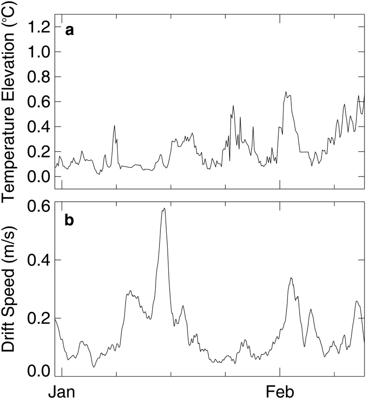
(a) R-Buoy temperature elevation of the water temperature above its in situ freezing point. The water temperature was measured from the radiometer thermistor mounted ~1.5 m below the ice and the freezing point temperature was the calculated freezing point temperature using the R-Buoy temperature and the S-Buoy CTD measurements of average salinity (see text). (b) R-Buoy drift speed with time, computed from differencing GPS positions taken at nominally hourly intervals, then smoothing with a 24 h running mean.

Drift speed
Drift speeds of the buoys were determined by differencing positions obtained by the onboard GPS on each buoy and using the Haversine formula to obtain distances on the curved Earth surface and then dividing by the time interval (usually hourly) between positions. A running mean (24 h) was then applied to this record to smooth out some of the speed errors that are otherwise magnified by small errors in positioning. The resulting smoothed drift speeds for the two buoys are shown in Figures 4b (S-Buoy) and 5b (R-Buoy).
Results
Changes in surface flooding depths
Figure 6 shows four thermistor time series (S-Buoy) initially in snow, distances shown are referenced to near the initial bottom boundary between flooded and dry snow: The thermistor at 0 cm (T11) is near the snow–ice interface at the time of placement; above it in the snow at 10 cm intervals are: +10 cm (T10), +20 cm (T9) and +30 cm (T8). Nearest the top of the snow, at +30 cm (T8) in Figure 6 illustrates the response of a sensor that remained in snow for nearly the entire record. The record for +30 cm (T8) initially shows strong temperature cycling with some solar heating response as its temperature cycles above and below 0oC, as 0oC is the upper limit of temperature in the snow at the snow melting point if shielded from the sun, until 14 January. Generally, its temperature continues to cycle but only up to −1°C until late in the record (28 January–3 February) when this snow temperature, in response to continuing cold air temperatures, cycles below −2°C, while still maintaining a diurnal cycle. The bottom curve, at 0 cm (T11) however, became flooded around 6 January as its temperature dropped to ~−1.7oC and stayed there throughout the record. Little variability is seen there, as the flooded layer provides a latent heat sink as an ice-water bath at a constant temperature, so only phase change, and not temperature change, occurs as heat is conducted into it from above, and therefore, the air diurnal temperature cycles seen in the snow above are not seen here. Similarly, the thermistors between show flooding at +10 cm (T10) on 16 January and +20 cm (T9) on 28 January, and finally, +30 cm (T8) on 4 February, when it appears over half the full depth (0.60 m) of the snowpack was flooded. A similar analysis of the R-Buoy thermistor records (not shown) indicates flooding of similar magnitude (~20–30 cm) during the same period in its thinner snowpack of 0.4 m total depth. With the relatively coarse spacing (10 cm) for the thermistors, there is however uncertainty in the precise level of surface flooding within that 10 cm level from these records.
S-Buoy temperatures with time for distances from the snow–sea-ice interface 0 cm (T11, 0 cm), 10 cm above the interface (T10, +10 cm), 20 cm above the interface (T9, +20 cm) and 30 cm above the interface (T8, +30 cm). Flooding events are indicated by temperatures reaching ~−1.7°C and remaining there. (Note that +30 cm (T8) reached below −1.7°C on 24 Jan, but both warmed and cooled from that time as it was still in snow, until plateauing at −1.7°C on 4 Feb when it became flooded with sea water.)

The level of flooding can also be determined through consideration of isostatic balance. The isostatic balance equation, where mass of water displaced equals the combined mass of ice, snow and slush, is:

where ρ w, ρ s, ρ sl, ρ i are the densities of sea water, snow, slush and ice, respectively, and tis the ice thickness, d is the slush depth and s is the snow depth. We use 1030 kg m−3 for sea-water density, 940 kg m−3 for ice density (Weeks and Ackley, Reference Weeks, Ackley and Untersteiner1986), 300 kg m−3 for snow density (Lewis and others, Reference Lewis2011) and 940 kg m−3 for slush density (Lewis and others, Reference Lewis2011). During the flooding process, we assume that snow compaction takes place such that the flooding snow is at least 50% ice by volume (Jeffries and others, Reference Jeffries, Krouse, Hurst-Cushing and Maksym2001), so we set the slush density the same as the warm ice density. This slush density of 940 kg m−3 was also computed when initial field measured values of snow depth, slush depth and ice thickness were used and Eqn (6) solved for the slush density instead of the slush depth. Solving Eqn (6) for the slush depth in mid-February after 1 m of ice loss on the R-Buoy gives a slush depth of 0.35 m or an increase of slush depth of 0.27 m, a value for flooded depth increase in agreement with that determined from the thermistor string records, of between 0.20 and 0.30 m, within their resolution.
Ice thickness changes from bottom melting
Figure 7a (R-Buoy) shows the ice thickness changes computed from the upward looking sonar data (every 4 h) plotted versus days in January and February. As shown in Figure 3c, the ice thickness stopped decreasing and leveled off to a constant value after 9 February. Total ice thickness change between the start of record (30 December) and end of the melting (around 9 February) was ~1.1 m. As shown in Figure 7a, the ice loss change was divided into five separate periods (by eye) and the data were linearly regressed for each of those periods. The slope of the line is given in m d−1 (Table 2) and varied from a high of 0.068 m d−1 in mid-January (Period 3) to a low of 0.011 m d−1 later in January (Period 4). Period 2 (early January) showed no change within the accuracy of the sonar (estimated at 0.02 m, Ackley and others, Reference Ackley, Xie and Tichenor2015) but is the shortest record (1–2 d), so is not considered. In Figure 7b, the ice thickness changes are shown for the S-Buoy over the same time period. (Days are included here from 3 February to 7 February, not shown in Fig. 2c.) For the S-Buoy, due to the presence of considerable data variability probably caused by a larger rms bottom roughness, only two periods were separable. The variability in sonar return for the ice bottom was probably due to a rougher bottom that melted differentially at the S-Buoy site, compared to a more level, more evenly melting undersurface at the R-Buoy. At the rougher bottom surface, the first sonar return would depend on the distance from the first normal surface to the incoming wave, which may not be the closest point to the sonar. If the angle changed slightly as the block surface melted, then the return may come from a different point that was then flatter and that surface may be 20 cm or more closer to or further away than the initial point. As the angle can change back, the initial surface may again be the reflecting surface so the ice thickness measurements may show high variability that is inconsistent with large changes in actual ice thickness over short periods of time. Over a several week long period however, the trend of the ice thickness changes (Fig. 7b) can effectively show the longer term change due to bottom melting.
(a) R-Buoy ice thickness with time (1 Jan–10 Feb). Linear regression lines with slopes indicative of ice melting rates in cm d−1 are shown for five segments of the data. Ice thickness changes at four-hourly intervals were determined from an upward-looking sonar mounted ~0.85 m below the initial ice bottom. (b) S-Buoy ice thickness with time (10 Jan–7 Feb). Linear regression lines with slopes indicative of ice melting rates in cm d−1 are shown for two segments of the data. Ice thickness changes at four-hourly intervals were determined from an upward-looking sonar mounted ~0.85 m below the initial ice bottom.

Melt rates (m d−1) of the two buoys in different time periods

From 10 January to 1 February, ice melt was generally much lower (0.014 m d−1) than the corresponding period for the R-Buoy (Table 2). As the S-Buoy approached the ice edge in early February, the melt rate increased to 0.065 m d−1, so the overall average melt rates for the two buoys over the entire period of overlap became much closer (last column in Table 2.).
Ocean heat flux from ocean property measurements
Ocean heat fluxes calculated for the S-Buoy and R-Buoy are shown in Figure 8, found with Eqn (2) using the temperature elevation above the freezing point (Figs 4a and 5a) and the drift speed (Figs 4b and 5b) at each co-measured point. The drift speed is used rather than a (scaled) u* in Eqn (2), although strictly speaking, the relative drift speed (the difference between the ice velocity and the surface ocean current) should be used, so ocean currents are presumed small compared to drift velocity in our approximation. For the R-Buoy, in order to calculate ocean heat flux from under-ice water temperatures and drift speeds, we used the average salinity derived from the salinity measurements on the S-Buoy to calculate the freezing point temperature. In order to determine how this affects the ocean heat flux calculation, we computed the difference between the heat flux determined using the S-Buoy instantaneous freezing point temperature compared to the heat flux determined using the S-Buoy average freezing point temperature. This difference is shown in Figure 8 (inset) as the absolute difference for each point. With few exceptions, the difference is <2 W m−2, that is an average absolute error of only ±2 W m−2. These errors in heat flux due to the average freezing point assumption are therefore small compared to the magnitude of the temperature elevation and introduce tolerable error (discussed further in the next section) for warmer water temperatures. When the temperature is close to the freezing point, even though the error as a percentage of the heat flux may be large, the actual heat flux is also small and only results in small ice thickness change errors.
Ocean heat flux determined with time (31 Dec 2010–13 Feb 2011) from the S-Buoy (red line). The ocean heat flux was determined using the temperature and in situ freezing point determined from the measurements of conductivity, temperature and pressure (depth) made by the CTD. Ocean heat flux determined with time (22 Dec 2010–13 Apr 2011) for the R-Buoy (blue line). The ocean heat flux was determined from the water temperature while the freezing point temperature used was the average value determined using the average salinity derived from the SeaBird conductivity record (33.3 psu). Ocean heat flux was nearly zero at the beginning (22 Dec–29 Dec 2010) and end (20 Mar–13 Apr 2011) of the records. (Note from Fig. 3 that temperatures within the ice are colder than the freezing points at these times also.) The smaller inset figure shows ocean heat flux error for the S-Buoy with time, determined by differencing (absolute) the ocean heat flux determined from in situ freezing point with the ocean heat flux determined by using the average salinity for the entire record (31 Dec 2010–13 Feb 2011) to determine a single average freezing point temperature. The average error is ~2 W m−2.

In order to compare the ocean heat flux from the ice thickness changes with that from the ocean measurements, the average of the ocean heat flux of the S-Buoy in Figure 8 (red line) from January 10 to February 1 is 19 W m−2, compared to an estimated 40 W m−2 from ice thickness regression (1.4 cm d−1). From 1 February until 7 February, the average S-Buoy ocean heat flux is 82 W m−2, compared to an estimated ~200 W m−2 from ice thickness change (6.5 cm d−1).
In Figure 8, the estimate for the R-Buoy of ocean heat flux (shown as the blue line) is similarly made. Comparing the R-Buoy ocean heat flux with ice thickness changes, the average ocean heat flux computed from 1 January to 10 February is 55 W m−2, compared to an estimated 79 W m−2 ocean heat flux from measured ice thickness rate change of ~2.7 cm d−1.
Discussion
Differences in heat flux derived from ocean properties and ice thickness determinations
The comparison between the estimated ocean heat flux from ice thickness changes gave larger values for the heat flux compared to ocean heat flux computed from ocean temperature and properties. Expressed in melt rates, the ocean heat flux during January from S-Buoy ocean properties would give a melt rate of only 0.6 cm d−1 compared to measured melt rate of 1.4 cm d−1 from ice thickness changes. From the R-Buoy during January, an ocean heat flux-derived melt rate would be ~2 cm d−1 compared to the melt rate from measured ice thickness change of 2.7–2.8 cm d−1. One of the reasons for this discrepancy may be the latent heat value used for the ice (Eqn (3); Ono, Reference Ono1968). If, instead, the sea ice has undergone a significant amount of interior melt deterioration, it may structurally have cm-sized brine channels as observed previously in cores taken at the end of summer in the Weddell Sea pack ice (Weeks and Ackley, Reference Weeks, Ackley and Untersteiner1986). As this deteriorated ice melts from below, this ice cover could have a smaller apparent latent heat per unit volume and may instead respond as shown here with a higher melt rate than a more intact ice cover would respond to the same ocean heat flux. The error from freezing point temperature changes is apparently small as estimated in Figure 8 and discussed earlier. The data point variations in the ice thickness regression plots (Fig. 7) show that there can be significant (and probably spurious short-term variation) uncertainty in the sonar-determined ice bottom profile that may also make it difficult to determine the ice thickness changes over short times. This variation is probably due to the variable reflection properties of a rough ice bottom as discussed earlier.
The ocean heat flux determination from ocean properties relies on a literature-derived value for the coefficient (Morison, Reference Morison1995; McPhee and others, Reference McPhee, Kottmeier and Morison1999), and uses a constant scaling between ice drift speed and friction velocity. This may be a poor approximation as this relationship depends on ice bottom conditions (rough or smooth) which cannot be independently determined here. Ice drift speed, water salinity profile (stability) and other factors may also change the heat transfer coefficient (e.g. Morison, Reference Morison1995; McPhee and others, Reference McPhee, Kottmeier and Morison1999). However, Ackley and others (Reference Ackley, Xie and Tichenor2015), for similar comparisons of ice thickness changes and bulk parameterization of ocean heat flux from Antarctic IMB buoy measurements in spring and fall, found instead good agreement between the two ocean heat flux determinations using the same heat transfer coefficients as here. With the absence of direct measurements, particularly of drag coefficients, whether changes in the coefficients or the porosity changes in the ice account for the differences is indeterminate at this point. It may also instead be a combination of both these factors.
Summer surface flooding processes in the Amundsen Sea ice pack
Mechanisms previously discussed for surface flooding, particularly for the Amundsen Sea region, focused their attention on winter increases in snow depth causing the ice surface to be pushed below sea level and causing sea water to intrude (Maksym and Jeffries, Reference Maksym and Jeffries2000; Perovich and others, Reference Perovich2004). We investigated instead an increase in surface flooding depth in summer due to ice bottom melting. The mechanism in summer for increasing the depth of flooding was caused by the substantial decrease in ice thickness which progressively raised the sea level into the snow cover to maintain isostatic balance in the floe. The process to increase the depth of the flooded layer was vertical in nature and did not require additional snowfall. At the end of the summer period for both the R-Buoy and S-Buoy sites, a total of ~0.3–0.35 m of flooded snow was found for each site.
Warm surface water as the source of high ocean heat fluxes in the summer pack ice zone
Water temperatures for the R-Buoy (Fig. 3d, bottom), an average of 0.47°C above the freezing point temperature (from 1 January to 10 February), showed high values starting near the end of December and continuing through early February, when cooling back to the freezing point commenced from about mid-February and continued until April. Water temperatures were generally cooler for the S-Buoy (Fig. 2d) (average of 0.21°C above the freezing point from 1 January until 9 February) and, particularly, were cooler during the mid-January period of peak temperatures for both buoys. In spring and fall, however, Ackley and others (Reference Ackley, Xie and Tichenor2015) found near surface water temperature freezing point elevation was <0.10°C, or two to five times lower than these summer values in the Amundsen Sea. The difference in water temperatures (Figs 2d and 3d), higher for the R-Buoy, suggests the water temperatures for the two buoys, despite being in a similar area oceanographically, were controlled by ice concentration differences that the two buoys encountered. Figure 1 shows the ice concentration map on 11 January, derived from passive microwave satellite data (Cavalieri and others, Reference Cavalieri, Parkinson, Gloersen and Zwally1996), and the buoy tracks of the two buoys. We analyzed the ice concentration variations by taking the daily ice concentration at each buoy position. This analysis showed on average 20% less ice concentration at the R-Buoy site than the S-Buoy site from 1 January through mid-January. The R-Buoy was closer to the coast during mid-January where offshore winds generally kept ice away (a coastal polynya), resulting in lower ice concentration (Fig. 1). Because of its lower albedo, the higher amount of open water absorbed more solar radiation prior to and during the buoy drift through the region leading to the warmer water temperatures on the R-Buoy track (Fig. 5). The S-Buoy drift was more offshore over waters covered with ice of higher ice concentration (Fig. 1) and resulted in lower temperatures and lower ocean heat flux along the S-Buoy's path during January.
The low snow accumulation (<10 cm) observed during January and February (Figs 2c and 3c) showed that other observations (e.g. Perovich and others, Reference Perovich2004) showing surface flooding controlled by precipitation in other seasons (spring) was not seen in summer here. For the R-Buoy site, 1.1 m of bottom melt caused by high ocean heat flux also created ~0.3–0.35 m of flooded snow. In March–April, the flooded layer on the R-Buoy site was lowered in temperature and therefore froze as snow ice (Fig. 3c). The total thickness at this time was ~1.1–1.2 m of sea ice with ~25% (0.3–0.35 m) added on as this new snow ice. Measurements of cores taken further west in the outflow regions of the eastern Amundsen Sea have found, on average, larger percentages of snow ice (~30%) than found in other areas of Antarctica (Jeffries and others, Reference Jeffries, Li, Jana, Krouse, Hurst-Cushing and Jeffries1998; Ackley and others, Reference Ackley2003). These larger percentages of snow ice are therefore commensurate with summer bottom melting causing increased flooding, followed by fall freeze-up, as well as possibly greater winter snowfall in the Amundsen Sea than elsewhere (e.g. Maksym and Markus, Reference Maksym and Markus2008). For the offshore S-Buoy site, ocean heat flux values offshore, while lower, still averaged 18.4 W m−2 during January and were similar to SHEBA mass-balance sites in the Arctic where values increased to more than 15 W m−2 during summer (Perovich and Elder, Reference Perovich and Elder2002). The Arctic warming was also attributed to solar heating of the waters in lower ice concentrations and caused high levels of bottom sea-ice melt there.
Conclusions
The variation in water temperature between the two buoy tracks and resulting differences in ocean heat flux-induced bottom melting illustrate the strong control that ice concentration variations have on the process of surface flooding caused by bottom melting in summer. While these measurements are presently only from the Amundsen Sea pack ice, there is implied dependence of water temperature and summer ocean heat flux on ice concentration, rather than regional water mass properties. This behavior suggests that remote sensing and an ice dynamics model, through ice concentration and water temperature predictions, can provide some estimates of bottom melting and surface flooding in summer ice conditions on a wider basis in both the Antarctic and Arctic pack ice zones for climate and biogeochemistry models. Still, additional year-round deployments of IMB buoys, together with high-resolution modeling and remote-sensing analyses over the buoy sites, are needed to better quantify these relationships and for validation of their derivation from these modeling or remote-sensing analyses.
Acknowledgement
This work was supported by the National Science Foundation grant to UTSA, ANT-0839053-Sea Ice System in Antarctic Summer (S.F. Ackley, H. Xie and B. Weissling), and to WHOI, ANT-1341513 (T. Maksym), and by the NASA Center for Advanced Measurements in Extreme Environments or NASA-CAMEE at UTSA, NASA #80NSSC19M0194 (S.F. Ackley, H. Xie, B.Weissling).
Author contribution
D.P. constructed and calibrated the IMBs and reduced the buoy data. B.W. installed the buoys in the Amundsen Sea pack ice. S.A. and H.X. conducted the analyses with assistance from T.M., D.P. and B.W. S.A wrote the first draft of the paper and all authors contributed to rewriting, figure production and editing.


 Open access