


1. Introduction
Magnetic reconnection is an ubiquitous process in magnetised plasmas that involves fast, explosive rearrangements of the magnetic field topology, resulting in the conversion of magnetic energy into thermal and kinetic energy (Yamada, Kulsrud & Ji Reference Yamada, Kulsrud and Ji2010; Zweibel & Yamada Reference Zweibel and Yamada2016; Hesse & Cassak Reference Hesse and Cassak2020; Ji et al. Reference Ji, Daughton, Jara-Almonte, Le, Stanier and Yoo2022). It drives some of the most energetic events in our solar system such as solar flares (Coppi & Friedland Reference Coppi and Friedland1971; Priest Reference Priest1986; Forbes Reference Forbes1991), coronal mass ejections (Gosling, Birn & Hesse Reference Gosling, Birn and Hesse1995) and geomagnetic storms (Phan, Paschmann & Sonnerup Reference Phan, Paschmann and Sonnerup1996). Magnetic reconnection has also been hypothesised to be responsible for the high-energy radiation observed from many extreme astrophysical environments, such as black hole accretion disks and their coronae (Goodman & Uzdensky Reference Goodman and Uzdensky2008; Beloborodov Reference Beloborodov2017; Werner, Philippov & Uzdensky Reference Werner, Philippov and Uzdensky2019; Ripperda, Bacchini & Philippov Reference Ripperda, Bacchini and Philippov2020; Hakobyan et al. Reference Hakobyan, Levinson, Sironi, Philippov and Ripperda2025), jets from active galactic nuclei (Giannios, Uzdensky & Begelman Reference Giannios, Uzdensky and Begelman2009; Nalewajko, Begelman & Sikora Reference Nalewajko, Begelman and Sikora2014; Sironi, Petropoulou & Giannios Reference Sironi, Petropoulou and Giannios2015; Mehlhaff et al. Reference Mehlhaff, Werner, Uzdensky and Begelman2020; Petropoulou, Psarras & Giannios Reference Petropoulou, Psarras and Giannios2023), pulsar wind nebulae (Uzdensky, Cerutti & Begelman Reference Uzdensky, Cerutti and Begelman2011; Schoeffler et al. Reference Schoeffler, Grismayer, Uzdensky and Silva2023; Cerutti et al. Reference Cerutti, Uzdensky and Begelman2012, Reference Cerutti, Werner, Uzdensky and Begelman2014; Cerutti & Philippov Reference Cerutti and Philippov2017), gamma ray bursts (Lyutikov Reference Lyutikov2006; Giannios Reference Giannios2008; McKinney & Uzdensky Reference McKinney and Uzdensky2012), pulsar magnetospheres (Lyubarsky & Kirk Reference Lyubarsky and Kirk2001; Uzdensky & Spitkovsky Reference Uzdensky and Spitkovsky2014; Cerutti et al. Reference Cerutti, Philippov, Parfrey and Spitkovsky2015, Reference Cerutti, Philippov and Spitkovsky2016; Philippov & Spitkovsky Reference Philippov and Spitkovsky2018; Philippov et al. Reference Philippov, Uzdensky, Spitkovsky and Cerutti2019; Hakobyan et al. Reference Hakobyan, Philippov and Spitkovsky2019, Reference Hakobyan, Philippov and Spitkovsky2023) and magnetar magnetospheres (Schoeffler et al. Reference Schoeffler, Grismayer, Uzdensky, Fonseca and Silva2019, Reference Schoeffler, Grismayer, Uzdensky and Silva2023).
For many of the aforementioned astrophysical environments, the energetic contribution of emitted radiation can introduce a myriad of effects such as radiative cooling (dominant in the optically thin regime), radiative drag forces and pair production (optically thick regime), which in turn impact the reconnection dynamics (Somov & Syrovatski Reference Somov and Syrovatski1976; Oreshina & Somov Reference Oreshina and Somov1998; Datta et al. Reference Datta2024b ). Additionally, remote telescopic observations of radiative emission driven by reconnection are often the only diagnostic probe into the dynamics of these extreme environments (Uzdensky Reference Uzdensky2011). Thus, a fundamental model of how radiation interacts with reconnection processes, starting with radiative cooling, is an essential part of understanding the microphysics that governs the behaviour of these radiation-rich astrophysical plasmas.
The importance of radiatively cooled reconnection motivated early numerical studies (Forbes & Malherbe Reference Forbes and Malherbe1991; Oreshina & Somov Reference Oreshina and Somov1998; Jaroschek & Hoshino Reference Jaroschek and Hoshino2009), which show a thinner, denser reconnection layer in the presence of radiative cooling, with slowed-down plasma outflows. More recently, radiative cooling has been included in large-scale particle-in-cell (PIC) simulations of the dynamics of astrophysical environments that are impacted by relativistic reconnection (Nalewajko, Yuan & Chruślińska Reference Nalewajko, Yuan and Chruślińska2018; Werner, Philippov & Uzdensky Reference Werner, Philippov and Uzdensky2018; Sridhar et al. Reference Sridhar, Sironi and Beloborodov2021, Reference Sridhar, Sironi and Beloborodov2023). Whilst there have been several analytic studies on the interaction of resistive tearing modes and radiation (Steinolfson Reference Steinolfson1983; Tachi, Steinolfson & Van Hoven Reference Tachi, Steinolfson and Van Hoven1983; van Hoven, Tachi & Steinolfson Reference van Hoven, Tachi and Steinolfson1984; Tachi, Steinolfson & Van Hoven Reference Tachi, Steinolfson and Van Hoven1985), the first theoretical description of radiatively cooled reconnection was provided by Uzdensky & McKinney (Reference Uzdensky and McKinney2011), building on previous work by Dorman & Kulsrud (Reference Dorman and Kulsrud1995). This description extends the Sweet–Parker (Parker Reference Parker1957, Reference Parker1963) model to account for compressibility due to radiative cooling and predicts the generation of a strongly compressed, colder reconnection layer, which is consistent with results from early simulations (Forbes & Malherbe Reference Forbes and Malherbe1991; Oreshina & Somov Reference Oreshina and Somov1998; Jaroschek & Hoshino Reference Jaroschek and Hoshino2009). Beyond the Sweet–Parker model, recent simulations (Sen & Keppens, Reference Sen and Keppens2022; Schoeffler et al. Reference Schoeffler, Grismayer, Uzdensky and Silva2023; Datta et al. Reference Datta2024b ) and experimental work (Datta et al. Reference Datta2024 a) have studied the impact of radiative cooling on reconnection and the plasmoid instability (Loureiro & Uzdensky Reference Loureiro and Uzdensky2015), showing the susceptibility of the layer and the formed plasmoids to additional instabilities such as radiative collapse.
However, this is only a small part of the total picture; the understanding of radiatively cooled reconnection is in its infancy in comparison with that of reconnection in the classical setting. This paper aims to lay out the groundwork for a more complete theoretical understanding of reconnection in a regime dominated by optically thin radiative cooling by examining the impact of cooling on current sheet formation. This is achieved by revisiting and extending the simple magnetohydrodynamics (MHD) model of current sheet formation through X-point collapse detailed by Chapman & Kendall (Reference Chapman and Kendall1963) and later Syrovatskii (Reference Syrovatskii1971), by including a radiative cooling term in the equation of state. The results show that whilst radiative cooling accelerates the collapse of the X-point along the direction of the inflows, strong cooling can arrest the current sheet elongation in the outflow direction and even result in its reversal and collapse along the outflow direction as well. In context of these results, a steady-state solution for radiatively cooled magnetic reconnection is derived by modifying the model developed by Uzdensky & McKinney (Reference Uzdensky and McKinney2011) to account for varying current sheet length. This is achieved by enforcing an extra condition, requiring the characteristic outflow time to be similar to the cooling time such that a plasma parcel in the layer can be advected out of the layer before undergoing radiatively driven collapse. It is found that, for the strong radiative cooling that dominates compressional heating, the current sheet length is contracted compared with the system size whilst also yielding an increased reconnection rate as compared with the standard Sweet–Parker model.
This paper is organised as follows; § 2 details the derivation of the equations dictating radiatively cooled X-point collapse in the Lagrangian MHD framework, which we adopt for our analytic derivation. Section 3 shows the numerical solutions to the derived equations, analyses the asymptotic behaviour of these solutions and provides a physical interpretation for the same. Section 4 details the calculation used to derive the current sheet length and reconnection rate from our modification of the radiatively cooled Sweet–Parker model. Section 5 discusses the significance of the results.
2. Method
We aim to develop a simple model to understand current sheet formation in an ideal MHD plasma that is radiatively cooled by an optically thin cooling mechanism parameterised as
 $\dot {Q}_{\text{rad}} \sim \rho ^aT^b$
(Rybicki & Lightman Reference Rybicki and Lightman2007), where
$\dot {Q}_{\text{rad}} \sim \rho ^aT^b$
(Rybicki & Lightman Reference Rybicki and Lightman2007), where
 $\dot {Q}_{\text{rad}}$
is the volumetric power loss due to radiative cooling,
$\dot {Q}_{\text{rad}}$
is the volumetric power loss due to radiative cooling,
 $\rho$
is the plasma mass density and
$\rho$
is the plasma mass density and
 $T$
is the plasma temperature.Footnote
1
The plasma is modelled to be compressible, whilst neglecting heat conduction and viscous heating. The equations governing this are
$T$
is the plasma temperature.Footnote
1
The plasma is modelled to be compressible, whilst neglecting heat conduction and viscous heating. The equations governing this are
 \begin{align}&\qquad\qquad\qquad \frac {\partial \rho }{\partial t}+\boldsymbol{\nabla } \boldsymbol{\cdot }(\rho \boldsymbol{v})=0, \end{align}
 \begin{align}&\qquad\quad \rho \left (\frac {\partial \boldsymbol{v}}{\partial t}+\boldsymbol{v} \boldsymbol{\cdot }\boldsymbol{\nabla } \boldsymbol{v}\right )=-\boldsymbol{\nabla } P+\frac {\boldsymbol{j} \times \boldsymbol{B}}{c}, \end{align}
 \begin{align}&\qquad\qquad\qquad\quad \frac {\partial \boldsymbol{B}}{\partial t}=\boldsymbol{\nabla } \times (\boldsymbol{v} \times \boldsymbol{B}), \end{align}
 \begin{align}& \frac {\partial P}{\partial t}=-(\gamma P \boldsymbol{\nabla }\boldsymbol{\cdot }\boldsymbol{v}+\boldsymbol{v}\boldsymbol{\cdot }\boldsymbol{\nabla }P)-(\gamma -1)C_{\text{cool}}\rho ^aT^b , \end{align}
where
 $\boldsymbol{B}$
is the magnetic field,
$\boldsymbol{B}$
is the magnetic field,
 $P$
is the plasma pressure,
$P$
is the plasma pressure,
 $\boldsymbol{v}$
is the fluid velocity,
$\boldsymbol{v}$
is the fluid velocity,
 $c$
is the speed of light and the current density
$c$
is the speed of light and the current density
 $\boldsymbol{j}$
is defined using Ampère’s law
$\boldsymbol{j}$
is defined using Ampère’s law
 $\boldsymbol{j}=c(\boldsymbol{\nabla }\times \boldsymbol{B})/4\pi$
. Here, the values of
$\boldsymbol{j}=c(\boldsymbol{\nabla }\times \boldsymbol{B})/4\pi$
. Here, the values of
 $a$
,
$a$
,
 $b$
and the cooling constant
$b$
and the cooling constant
 $C_{\text{cool}}$
are specific to the cooling mechanism considered. In the case of thermal bremsstrahlung radiation,
$C_{\text{cool}}$
are specific to the cooling mechanism considered. In the case of thermal bremsstrahlung radiation,
 $a=2$
,
$a=2$
,
 $b=1/2$
, yielding
$b=1/2$
, yielding
 $C_{\text{cool}}\rho ^2T^{1/2}\approx 8.3\times 10^{26}\rho ^2T^{1/2}[\text{erg s}^{-1}\text{cm}^{-3}]$
.Footnote
2
$C_{\text{cool}}\rho ^2T^{1/2}\approx 8.3\times 10^{26}\rho ^2T^{1/2}[\text{erg s}^{-1}\text{cm}^{-3}]$
.Footnote
2
2.1. Lagrangian MHD
Following the formalism laid out by Newcomb (Reference Newcomb1961), as detailed in Schekochihin (Reference Schekochihin2025), Lagrangian MHD reformulates the MHD equations into the frame of reference of the fluid parcel. This is particularly useful as it results in a single equation of motion relying solely on the Eulerian fields prescribed at
 $t=0$
.
$t=0$
.
To derive this Lagrangian equation of motion, we start by defining the relevant frames of reference;
 $\boldsymbol{r}_0$
is defined as the Lagrangian coordinate with a corresponding Eulerian coordinate
$\boldsymbol{r}_0$
is defined as the Lagrangian coordinate with a corresponding Eulerian coordinate
 $\boldsymbol{r}=\boldsymbol{r}_0+\boldsymbol{\epsilon }(t,\boldsymbol{r}_0)$
, where
$\boldsymbol{r}=\boldsymbol{r}_0+\boldsymbol{\epsilon }(t,\boldsymbol{r}_0)$
, where
 $\boldsymbol{\epsilon }(t,\boldsymbol{r}_0)$
is the displacement of the fluid parcel from its initial position in the Eulerian frame. Using this definition along with the known expression for convective derivatives
$\boldsymbol{\epsilon }(t,\boldsymbol{r}_0)$
is the displacement of the fluid parcel from its initial position in the Eulerian frame. Using this definition along with the known expression for convective derivatives
 $\partial /\partial t_L={\rm d}/{\rm d}t\equiv \partial /\partial t+\boldsymbol{v}\boldsymbol{\cdot }\boldsymbol{\nabla }$
, where the subscript ‘
$\partial /\partial t_L={\rm d}/{\rm d}t\equiv \partial /\partial t+\boldsymbol{v}\boldsymbol{\cdot }\boldsymbol{\nabla }$
, where the subscript ‘
 $L$
’ denotes quantities in the Lagrangian frame, one can then evaluate the velocities
$L$
’ denotes quantities in the Lagrangian frame, one can then evaluate the velocities
 \begin{equation} \partial _t \boldsymbol{r}\left (t, \boldsymbol{r}_0\right )=\partial _t \boldsymbol{\epsilon }\left (t, \boldsymbol{r}_0\right ) \rightarrow \boldsymbol{v}(t, \boldsymbol{r})=\boldsymbol{v}_L\left (t, \boldsymbol{r}_0\right )\!, \end{equation}
and spatial derivatives
 \begin{equation} \boldsymbol{\nabla }_0=\left (\boldsymbol{\nabla }_0 \boldsymbol{r}\right ) \boldsymbol{\cdot }\boldsymbol{\nabla }=\left (\mathbb{I}+\boldsymbol{\nabla }_0 \boldsymbol{\epsilon }\right )\boldsymbol{\cdot }\boldsymbol{\nabla } ,\end{equation}
where
 $\mathbb{I}$
is the
$\mathbb{I}$
is the
 $N$
-dimensional identity matrix (here,
$N$
-dimensional identity matrix (here,
 $N=3$
).
$N=3$
).
Next, we define the Jacobian relating the Eulerian and Lagrangian frames
 \begin{equation} J\left (t,\boldsymbol{r}_0\right )=\left |\operatorname {det} \boldsymbol{\nabla} _0 \boldsymbol{r}\right |=\frac {1}{6} \varepsilon ^{i j k} \varepsilon ^{l m n} \frac {\partial r_i}{\partial r_{0 l}} \frac {\partial r_j}{\partial r_{0 m}} \frac {\partial r_k}{\partial r_{0 n}} \rightarrow \text{d} \boldsymbol{r}=J\left (t,\boldsymbol{r}_0\right ) \text{d} \boldsymbol{r}_0. \end{equation}
This expression for
 $J(t,\boldsymbol{r}_0)$
, along with the prescribed definitions for velocities and time and spatial derivatives, is everything required to convert all the relevant MHD fields to their Lagrangian counterparts, which will now be denoted using the subscript ‘
$J(t,\boldsymbol{r}_0)$
, along with the prescribed definitions for velocities and time and spatial derivatives, is everything required to convert all the relevant MHD fields to their Lagrangian counterparts, which will now be denoted using the subscript ‘
 $L$
’.
$L$
’.
As an example, an expression for the Lagrangian mass density
 $\rho _L(t,\boldsymbol{r}_0)$
can be derived in terms of
$\rho _L(t,\boldsymbol{r}_0)$
can be derived in terms of
 $\rho _0(\boldsymbol{r}_0)=\rho (t=0,\boldsymbol{r}_0)$
by substituting
$\rho _0(\boldsymbol{r}_0)=\rho (t=0,\boldsymbol{r}_0)$
by substituting
 $J(t,\boldsymbol{r}_0)$
in the continuity equation
$J(t,\boldsymbol{r}_0)$
in the continuity equation
 \begin{equation} \begin{aligned} &\rho _0\left (\boldsymbol{r}_0\right ) {\rm d} \boldsymbol{r}_0=\rho (t,\boldsymbol{r}) {\rm d} \boldsymbol{r}=\rho _L\left (t,\boldsymbol{r}_0\right ) {\rm d} \boldsymbol{r}= \rho _L\left (t,\boldsymbol{r}_0\right ) J(t,\boldsymbol{r}_0){\rm d} \boldsymbol{r}_0, \\ & \Rightarrow \rho _L\left (t, \boldsymbol{r}_0\right )=\frac {\rho _0\left (\boldsymbol{r}_0\right )}{J\left (t,\boldsymbol{r}_0\right )}. \end{aligned} \end{equation}
Similarly, we can use the induction equation and adiabatic equation of state to obtain corresponding Lagrangian expressions for the magnetic field,
 $\boldsymbol{B}_L (t,\boldsymbol{r}_0)$
 \begin{equation} \boldsymbol{B}_{L}(t,\boldsymbol{r}_0)=\frac {\boldsymbol{B}_0\left (\boldsymbol{r}_0\right ) \boldsymbol{\cdot }\boldsymbol{\nabla} _0 \boldsymbol{r}\left (t, \boldsymbol{r}_0\right )}{J\left (t, \boldsymbol{r}_0\right )}, \end{equation}
and pressure,
 $P_L\left (t, \boldsymbol{r}_0\right )$
 \begin{equation} P_L\left (t, \boldsymbol{r}_0\right )=\frac {P_0}{J^\gamma \left (t, \boldsymbol{r}_0\right )}. \end{equation}
Plugging all these quantities into the momentum equation yields the following equation of motion, entirely expressed in terms of the Jacobian
 $J\left (t, \boldsymbol{r}_0\right )$
and initial field values:
$J\left (t, \boldsymbol{r}_0\right )$
and initial field values:
 \begin{equation} \frac {\rho _0}{J} \frac {\partial ^2 \boldsymbol{r}}{\partial t^2}=-\left (\boldsymbol{\nabla }_0 \boldsymbol{r}\right )^{-1} \boldsymbol{\cdot }\boldsymbol{\nabla }_0\left (\frac {P_0}{J^\gamma }+\frac {\left |\boldsymbol{B}_0 \boldsymbol{\cdot }\boldsymbol{\nabla }_0 \boldsymbol{r}\right |^2}{8 \pi J^2}\right )+\frac {1}{4 \pi } \frac {\boldsymbol{B}_0}{J} \boldsymbol{\cdot }\boldsymbol{\nabla }_0 \frac {\boldsymbol{B}_0}{J} \boldsymbol{\cdot }\boldsymbol{\nabla }_0 \boldsymbol{r}. \end{equation}
2.2. Background: X-point collapse
Current sheet formation through X-point collapse in an ideal MHD plasma has been extensively studied in the past, with the most notable solutions for an incompressible plasma, as derived by Chapman & Kendall (Reference Chapman and Kendall1963), describing the exponential growth of current density
 $j$
. However, to include the impact of radiative cooling, the plasma considered is required to be compressible. This can be understood by considering the instantaneous pressure imbalance introduced due to radiative cooling; cooling results in a drop in thermal pressure, resulting in the compression of the cooled plasma by the inward magnetic pressure as a response. The calculation that includes plasma compressibility and spatially uniform pressure with the generalised equation of state
$j$
. However, to include the impact of radiative cooling, the plasma considered is required to be compressible. This can be understood by considering the instantaneous pressure imbalance introduced due to radiative cooling; cooling results in a drop in thermal pressure, resulting in the compression of the cooled plasma by the inward magnetic pressure as a response. The calculation that includes plasma compressibility and spatially uniform pressure with the generalised equation of state
 $P=P(\rho )$
was performed by Syrovatskii (Reference Syrovatskii1971), and will be referred to as S71 for the rest of this paper.
$P=P(\rho )$
was performed by Syrovatskii (Reference Syrovatskii1971), and will be referred to as S71 for the rest of this paper.
The calculation in S71 is approached in the Eulerian frame of reference with the following initial conditions describing a standard X-point configuration with flows in the
 $x-y$
plane:
$x-y$
plane:
 \begin{align} \psi (x, y) & =\frac {1}{2}\left (x^2-y^2\right )\!, \nonumber\\[4pt] v_x(x, y) & =\varGamma _{x,0} x, \quad v_y(x, y)=\varGamma _{y,0} y, \nonumber\\[4pt] \rho (x, y) & =1, \end{align}
where
 $\varGamma _{x,0}$
and
$\varGamma _{x,0}$
and
 $\varGamma _{y,0}$
are the initial collapse rates along the
$\varGamma _{y,0}$
are the initial collapse rates along the
 $x$
-axis and
$x$
-axis and
 $y$
-axis respectively. Here, the X-point is expressed in terms of the magnetic flux function
$y$
-axis respectively. Here, the X-point is expressed in terms of the magnetic flux function
 $\psi$
, which has the standard definition
$\psi$
, which has the standard definition
 $\boldsymbol{B}_0=\boldsymbol{\hat {z}}\boldsymbol{\cdot} \boldsymbol{\nabla }_{\perp }\psi$
for a background field
$\boldsymbol{B}_0=\boldsymbol{\hat {z}}\boldsymbol{\cdot} \boldsymbol{\nabla }_{\perp }\psi$
for a background field
 $\boldsymbol{B}_0$
(and, thus,
$\boldsymbol{B}_0$
(and, thus,
 $\psi =-A_z$
, where
$\psi =-A_z$
, where
 $\mathbf{A}$
is the magnetic vector potential). Dimensionally,
$\mathbf{A}$
is the magnetic vector potential). Dimensionally,
 $\boldsymbol{B}_0$
has been normalised with respect to the upstream magnetic field
$\boldsymbol{B}_0$
has been normalised with respect to the upstream magnetic field
 $B_{\text{up}}$
and
$B_{\text{up}}$
and
 $x$
and
$x$
and
 $y$
have been normalised with respect to a characteristic length scale
$y$
have been normalised with respect to a characteristic length scale
 $L_{\text{sys}}$
. Velocities are normalised with respect to the Alfvén velocity
$L_{\text{sys}}$
. Velocities are normalised with respect to the Alfvén velocity
 $V_A\equiv B_{\text{up}}/(4\pi \rho _0)^{1/2}$
and times are normalised with respect to the Alfvén time
$V_A\equiv B_{\text{up}}/(4\pi \rho _0)^{1/2}$
and times are normalised with respect to the Alfvén time
 $\tau _A\equiv L_{\text{sys}}/V_A$
. Additionally, it is noted that the spatial uniformity of pressure is implied by the condition
$\tau _A\equiv L_{\text{sys}}/V_A$
. Additionally, it is noted that the spatial uniformity of pressure is implied by the condition
 $\rho (x,y)=1$
, which is expressed in normalised units.
$\rho (x,y)=1$
, which is expressed in normalised units.
For these initial conditions, the MHD equations allow exact similarity solutions, expressed as follows:
 \begin{align} \psi (x, y, t) & =\frac {1}{2}\left (\frac {x^2}{\xi ^2(t)}-\frac {y^2}{\eta ^2(t)}\right )\!, \nonumber\\[3pt] v_x(x, y, t) & =\varGamma _x(t) x, \quad v_y(x, y, t)=\varGamma _y(t) y, \nonumber\\[3pt] \rho (x, y, t) & =\rho (t). \end{align}
Substituting these expressions into the MHD equations above ((2.1)–(2.4) with
 $C_{\text{cool}}=0$
) yields the following equations relating
$C_{\text{cool}}=0$
) yields the following equations relating
 $\xi$
,
$\xi$
,
 $\eta$
,
$\eta$
,
 $\varGamma _x$
,
$\varGamma _x$
,
 $\varGamma _y$
and
$\varGamma _y$
and
 $\rho$
:
$\rho$
:
 \begin{align}&\qquad \dot {\rho }+\rho (\varGamma _x+\varGamma _y)=0,\\[-10pt]\nonumber \end{align}
 \begin{align}& \rho \big(\dot {\varGamma }_x+\varGamma _x^2\big)=-\frac {1}{\xi ^2}\left (\frac {1}{\xi ^2}-\frac {1}{\eta ^2}\right )\!, \nonumber\\[5pt] & \rho \big(\dot {\varGamma }_y+\varGamma _y^2\big)=\frac {1}{\eta ^2}\left (\frac {1}{\xi ^2}-\frac {1}{\eta ^2}\right )\!,\\[-13pt]\nonumber \end{align}
 \begin{align}&\qquad \dot {\xi }=\varGamma _x\xi , \quad \dot {\eta }=\varGamma _y \eta . \end{align}
Thus, combining (2.14)–(2.16) yields the following set of equations for
 $\xi$
and
$\xi$
and
 $\eta$
:
$\eta$
:
 \begin{align}& \ddot {\xi }=-\eta \left (\frac {1}{\xi ^2}-\frac {1}{\eta ^2}\right )\!, \end{align}
 \begin{align}& \ddot {\eta }=\xi \left (\frac {1}{\xi ^2}-\frac {1}{\eta ^2}\right )\!, \end{align}
with initial conditions
 $\xi _0=\eta _0=1, \dot {\xi }_0=\varGamma _{x,0}, \dot {\eta }_0=\varGamma _{y,0}$
. The solutions to this set of coupled equations completely prescribe the dynamics of the system. The numerical solutions (with
$\xi _0=\eta _0=1, \dot {\xi }_0=\varGamma _{x,0}, \dot {\eta }_0=\varGamma _{y,0}$
. The solutions to this set of coupled equations completely prescribe the dynamics of the system. The numerical solutions (with
 $\varGamma _x\lt 0$
and
$\varGamma _x\lt 0$
and
 $\varGamma _y\gt 0$
), as seen in figure 1, show that
$\varGamma _y\gt 0$
), as seen in figure 1, show that
 $\eta$
grows over time, while
$\eta$
grows over time, while
 $\xi$
collapses and exhibits a finite-time singularity, representing a forming current sheet with inflows and outflows along the
$\xi$
collapses and exhibits a finite-time singularity, representing a forming current sheet with inflows and outflows along the
 $x$
- and
$x$
- and
 $y$
-axes, respectively, and a diverging current density
$y$
-axes, respectively, and a diverging current density
 $j=(1/\xi ^2-1/\eta ^2)\to \infty$
(obviously, in a realistic system resistivity would eventually become important and kerb the growth of the current).
$j=(1/\xi ^2-1/\eta ^2)\to \infty$
(obviously, in a realistic system resistivity would eventually become important and kerb the growth of the current).
When performing this calculation in Lagrangian MHD, it can be seen that the equations for
 $\xi$
and
$\xi$
and
 $\eta$
can easily be recovered by considering the self-similar solution as a coordinate conversion
$\eta$
can easily be recovered by considering the self-similar solution as a coordinate conversion
 $x=\xi (t) x_0,\ y=\eta (t) y_0, \ z=z_0$
that is substituted into (2.11). Using this coordinate conversion, the following expressions can be obtained for
$x=\xi (t) x_0,\ y=\eta (t) y_0, \ z=z_0$
that is substituted into (2.11). Using this coordinate conversion, the following expressions can be obtained for
 $J$
:
$J$
:
 \begin{equation} J\left (t,\boldsymbol{r}_0\right )=\left |\operatorname {det} \boldsymbol{\nabla} _0 \boldsymbol{r}\right |=\frac {1}{6} \varepsilon ^{i j k} \varepsilon ^{l m n} \frac {\partial r_i}{\partial r_{0 l}} \frac {\partial r_j}{\partial r_{0 m}} \frac {\partial r_k}{\partial r_{0 n}}=\xi (t)\eta (t), \end{equation}
and for
 $\boldsymbol{\nabla }_0 \boldsymbol{r}$
and
$\boldsymbol{\nabla }_0 \boldsymbol{r}$
and
 $\left (\boldsymbol{\nabla }_0 \boldsymbol{r}\right )^{-1}$
 \begin{align} \boldsymbol{\nabla }_0 \boldsymbol{r}= \left[\begin{array}{c@{\quad}c} \xi &0\\[3pt] 0 & \eta \end{array}\right], \quad \left (\boldsymbol{\nabla }_0 \boldsymbol{r}\right )^{-1}=\left[\begin{array}{c@{\quad}c} 1/\xi &0\\[3pt] 0 & 1/\eta \end{array}\right]. \end{align}
Substituting these expressions into (2.11) exactly yields (2.17) and (2.18).
2.3. Lagrangian equation of motion with radiative cooling
Sticking to the Lagrangian formalism, we aim to find modified equations for
 $\xi$
and
$\xi$
and
 $\eta$
which include the effect of optically thin radiative cooling, by keeping the entire right-hand side of the equation of state (2.4). This implies that, whilst the coordinate conversions of density and magnetic field remain the same, the conversion of pressure changes such that it takes a form that satisfies the modified equation of state. To find this, we first recast the equation of state to isolate the cooling term and express it entirely in terms of pressure
$\eta$
which include the effect of optically thin radiative cooling, by keeping the entire right-hand side of the equation of state (2.4). This implies that, whilst the coordinate conversions of density and magnetic field remain the same, the conversion of pressure changes such that it takes a form that satisfies the modified equation of state. To find this, we first recast the equation of state to isolate the cooling term and express it entirely in terms of pressure
 $P$
and mass density
$P$
and mass density
 $\rho$
 \begin{equation} \frac {\rm d}{{\rm d} t} \ln \left [\frac {P}{\rho ^\gamma }\right ]=-(\gamma -1) C_{\text{cool}}\left [\frac {(Z+1)}{m_i+Zm_e}\right ]^{-b} \rho ^{a-b} P^{b-1}. \end{equation}
This additional factor of
 $[(Z+1)/(m_i+Zm_e)]^{-b}$
, where
$[(Z+1)/(m_i+Zm_e)]^{-b}$
, where
 $Z$
is the atomic number,
$Z$
is the atomic number,
 $m_i$
is the ion mass and
$m_i$
is the ion mass and
 $m_e$
is the electron mass, comes from converting number density
$m_e$
is the electron mass, comes from converting number density
 $n$
to mass density
$n$
to mass density
 $\rho$
.
$\rho$
.
Defining
 \begin{equation} \overline {C}_{\text{cool}} \equiv (\gamma -1) C_{\text{cool}}\left [\frac {(Z+1)}{m_i+Zm_e}\right ]^{-b}, \end{equation}
the corresponding Lagrangian equation of state is
 \begin{equation} \frac {\partial }{\partial t} \ln \left [\frac {P_L}{\rho _L^\gamma }\right ]=-\overline {C}_{\text{cool}} \rho _L^{a-b} P_L^{b-1}. \end{equation}
Given that
 $P_L\rho _L^{-\gamma }=P_0\rho _0^{-\gamma }$
at
$P_L\rho _L^{-\gamma }=P_0\rho _0^{-\gamma }$
at
 $t=0$
, we can use the ansatz
$t=0$
, we can use the ansatz
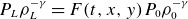 $P_L\rho _L^{-\gamma }=F(t,x,y)P_0\rho _0^{-\gamma }$
, with
$P_L\rho _L^{-\gamma }=F(t,x,y)P_0\rho _0^{-\gamma }$
, with
 $F(t=0,x,y)=1$
, in the equation of state to obtain the following general solution for
$F(t=0,x,y)=1$
, in the equation of state to obtain the following general solution for
 $P_L$
(solved in Appendix A):
$P_L$
(solved in Appendix A):
 \begin{equation} P_L=\frac {P_0}{J^\gamma } \left (C_1-\frac {C_2}{P_0}\left [(\gamma -1)(1-b) \overline {C}_{\text{cool}} \int _0^t J^{b(1-\gamma )+(\gamma -a)}(t',\boldsymbol{r}_0) \text{d} t^{\prime }\right ]^{1 /(1-b)}\right ). \end{equation}
Given that the initial conditions can entirely be satisfied by setting
 $C_1=1$
, the choice of
$C_1=1$
, the choice of
 $C_2(x_0,y_0)$
is unconstrained. It can be seen that
$C_2(x_0,y_0)$
is unconstrained. It can be seen that
 $C_2(x_0,y_0)$
is dimensionally a pressure term, thus, a sensible choice would be to set it to
$C_2(x_0,y_0)$
is dimensionally a pressure term, thus, a sensible choice would be to set it to
 $P_0(x_0,y_0)$
. To fully specify this solution, a pressure profile needs to be selected; for this, we choose to set a parabolic pressure profile
$P_0(x_0,y_0)$
. To fully specify this solution, a pressure profile needs to be selected; for this, we choose to set a parabolic pressure profile
 \begin{equation} P_0\left (x_0, y_0\right )=P_{0, X}\left (1-\frac {1}{2}\left (x_0^2+y_0^2\right )\right )\!, \end{equation}
where
 $P_{0,X}$
is a constant signifying the maximum magnitude of the pressure. This is physically similar to what would be expected in a reconnection layer, with the pressure and heating concentrated near the current sheet. With these choices, (2.24) yields the following final form for
$P_{0,X}$
is a constant signifying the maximum magnitude of the pressure. This is physically similar to what would be expected in a reconnection layer, with the pressure and heating concentrated near the current sheet. With these choices, (2.24) yields the following final form for
 $P_L$
:
$P_L$
:
 \begin{equation} P_L=\frac {P_0\left (x_0, y_0\right )}{J^\gamma }\left (1-\widetilde {C}_{\text{cool}}\left [ \int _0^t J^{b(1-\gamma )+(\gamma -a)}(t',\boldsymbol{r}_0) \text{d} t^{\prime }\right ]^{1 /(1-b)}\right )\!, \end{equation}
with all the relevant cooling constants absorbed into
 $\widetilde {C}_{\text{cool}}$
 \begin{equation} \widetilde {C}_{\text{cool}}=[(\gamma -1)(1-b)\overline {C}_{\text{cool}}]^{1/(1-b)}. \end{equation}
Plugging this into the momentum equation along with the standard definitions for
 $B_L$
and
$B_L$
and
 $\rho _L$
yields the following modified Lagrangian equation of motion:
$\rho _L$
yields the following modified Lagrangian equation of motion:
 \begin{align} \frac {\rho _0}{J} \frac {\partial ^2 \boldsymbol{r}}{\partial t^2}&=-\left (\boldsymbol{\nabla }_0 \boldsymbol{r}\right )^{-1} \boldsymbol{\cdot }\boldsymbol{\nabla }_0\left (\frac {P_0}{J^\gamma }\left [\widetilde {C}_{\text{cool}} I[J]^{1/(1-b)}-1\right ]+\frac {\left |\boldsymbol{B}_0 \boldsymbol{\cdot }\boldsymbol{\nabla }_0 \boldsymbol{r}\right |^2}{8 \pi J^2}\right )\nonumber\\[5pt]&\quad +\frac {1}{4 \pi } \frac {\boldsymbol{B}_0}{J} \boldsymbol{\cdot }\boldsymbol{\nabla }_0 \frac {\boldsymbol{B}_0}{J} \boldsymbol{\cdot }\boldsymbol{\nabla }_0 \boldsymbol{r}, \end{align}
where
 \begin{equation} I[J]=\int _0^t J^{b(1-\gamma )+(\gamma -a)}(t',\boldsymbol{r}_0) \text{d} t^{\prime }. \end{equation}
This expression notably differs from that in (2.11) by including an expression for pressure that is modified by radiative cooling and a non-uniform initial pressure by a factor of
 $\widetilde {C}_{\text{cool}} I[J]^{1/(1-b)}-1$
.
$\widetilde {C}_{\text{cool}} I[J]^{1/(1-b)}-1$
.
Starting with the same X-point configuration as S71 (2.12), a Lagrangian equation of motion that includes radiative cooling can be obtained by plugging in the coordinate conversion
 $x=\xi (t) x_0, \quad y=\eta (t) y_0, \quad z=z_0$
. Similar to § 2.2, substituting the expression for J (2.19) and
$x=\xi (t) x_0, \quad y=\eta (t) y_0, \quad z=z_0$
. Similar to § 2.2, substituting the expression for J (2.19) and
 $\boldsymbol{\nabla }_0 \boldsymbol{r}$
and
$\boldsymbol{\nabla }_0 \boldsymbol{r}$
and
 $\left (\boldsymbol{\nabla }_0 \boldsymbol{r}\right )^{-1}$
(2.20) into (2.28) yields the following matrix equation for
$\left (\boldsymbol{\nabla }_0 \boldsymbol{r}\right )^{-1}$
(2.20) into (2.28) yields the following matrix equation for
 $\xi$
and
$\xi$
and
 $\eta$
:
$\eta$
:
 \begin{equation} \frac {1}{\xi \eta } \begin{bmatrix} x_0\ddot {\xi }\\[3pt] y_0\ddot {\eta } \end{bmatrix} =-\frac {(\widetilde {C}_{\text{cool}} I[\xi \eta ]^{1/(1-b)}-1)}{(\xi \eta )^\gamma } \begin{bmatrix} \partial _{x_0}P_{0}/\xi \\[3pt] \partial _{y_0}P_{0}/\eta \end{bmatrix} + \begin{bmatrix} x_0/\xi ^3 \\[3pt] y_0/\eta ^3 \end{bmatrix} +\frac {1}{\xi \eta } \begin{bmatrix} x_0/\eta \\[3pt] y_0/\xi \end{bmatrix}. \end{equation}
Finally, a set of spatially independent coupled equations for
 $\xi$
and
$\xi$
and
 $\eta$
can be found using the selected form of
$\eta$
can be found using the selected form of
 $P_0\left (x_0, y_0\right )$
in (2.25)
$P_0\left (x_0, y_0\right )$
in (2.25)
 \begin{align} \ddot {\xi } & =-\eta \left [\frac {1}{\xi ^2}-\frac {1}{\eta ^2}+\frac {P_{0,X}(\widetilde {C}_{\text{cool}}\left (I[\xi \eta ]\right )^{{1}/{(1-b)}}-1)}{(\xi \eta )^\gamma }\right ], \nonumber\\[4pt] \ddot {\eta }& =\xi \left [\frac {1}{\xi ^2}-\frac {1}{\eta ^2}-\frac {P_{0,X}(\widetilde {C}_{\text{cool}}\left (I[\xi \eta ]\right )^{{1}/{(1-b)}}-1)}{(\xi \eta )^\gamma }\right ]. \end{align}
The equations derived in S71 ((2.17) and (2.18)) can be recovered by setting
 $\widetilde {C}_{\text{cool}}=0$
(no radiative cooling) and setting
$\widetilde {C}_{\text{cool}}=0$
(no radiative cooling) and setting
 $P_0$
to be uniform. Looking at the form of these equations, we can qualitatively anticipate what the impact of radiation would be. First considering the equation for
$P_0$
to be uniform. Looking at the form of these equations, we can qualitatively anticipate what the impact of radiation would be. First considering the equation for
 $\ddot {\xi }$
; given that the
$\ddot {\xi }$
; given that the
 $1/\xi ^2$
terms and cooling terms have the same sign, radiative cooling contributes to
$1/\xi ^2$
terms and cooling terms have the same sign, radiative cooling contributes to
 $\ddot {\xi }$
becoming more negative, implying that radiation accelerates the collapse of
$\ddot {\xi }$
becoming more negative, implying that radiation accelerates the collapse of
 $\xi$
. In the equation for
$\xi$
. In the equation for
 $\ddot {\eta }$
, the
$\ddot {\eta }$
, the
 $1/\xi ^2$
term and the cooling term have opposite signs;
$1/\xi ^2$
term and the cooling term have opposite signs;
 $\ddot {\eta }$
can become negative if the cooling term dominates over
$\ddot {\eta }$
can become negative if the cooling term dominates over
 $1/{\xi ^2}$
, resulting in the deceleration of the outflows.
$1/{\xi ^2}$
, resulting in the deceleration of the outflows.
To find a reasonable physical interpretation for
 $\widetilde {C}_{\text{cool}}$
, we re-express this term as a function of the cooling parameter
$\widetilde {C}_{\text{cool}}$
, we re-express this term as a function of the cooling parameter
 \begin{equation} R\equiv \frac {\tau _{\text{outflow}}}{\tau _{\text{cool}}}. \end{equation}
Here,
 $\tau _{\text{cool}}$
is the effective cooling time
$\tau _{\text{cool}}$
is the effective cooling time
 \begin{equation} \tau _{\text{cool }} \equiv \frac {P}{\dot {Q}_{\text{rad }}} \approx \frac {P^{1-b}\rho ^{b-a}}{\overline {C}_{\text{cool}}}, \end{equation}
and
 $\tau _{\text{outflow}}$
is the time scale corresponding to the advection of the outflows
$\tau _{\text{outflow}}$
is the time scale corresponding to the advection of the outflows
 \begin{equation} \tau _{\text{outflow}} =\frac {\eta }{v_y(y=\eta )}=\frac {1}{\varGamma _y} , \end{equation}
where
 $\eta$
is the characteristic length of the current sheet at a given time with a corresponding outflow velocity
$\eta$
is the characteristic length of the current sheet at a given time with a corresponding outflow velocity
 $\varGamma _y\eta$
;
$\varGamma _y\eta$
;
 $R$
is directly related to the strength of radiative cooling as it is a measure of how fast a fluid parcel can be radiatively cooled before it is advected away. For the configuration in this paper, the general definitions of
$R$
is directly related to the strength of radiative cooling as it is a measure of how fast a fluid parcel can be radiatively cooled before it is advected away. For the configuration in this paper, the general definitions of
 $\tau _{\text{cool}}$
and
$\tau _{\text{cool}}$
and
 $\tau _{\text{outflow}}$
are expected to be non-uniform and time dependent, thus
$\tau _{\text{outflow}}$
are expected to be non-uniform and time dependent, thus
 $\tau _{\text{cool}}$
and
$\tau _{\text{cool}}$
and
 $\tau _{\text{outflow}}$
in the expression for
$\tau _{\text{outflow}}$
in the expression for
 $R$
need to be defined at a specific time and position. We choose to define
$R$
need to be defined at a specific time and position. We choose to define
 $R$
at
$R$
at
 $t=0$
at the X-point, yielding
$t=0$
at the X-point, yielding
 \begin{equation} R=\overline {C}_{\text{cool}} \varGamma _{y,0}P_{0,X}^{b-1}\rho _0^{a-b}. \end{equation}
By rearranging this expression to isolate
 $\overline {C}_{\text{cool}}$
and substituting it in (2.27), the following relationship between
$\overline {C}_{\text{cool}}$
and substituting it in (2.27), the following relationship between
 $\widetilde {C}_{\text{cool}}$
and
$\widetilde {C}_{\text{cool}}$
and
 $R$
can be obtained:
$R$
can be obtained:
 \begin{equation} \widetilde {C}_{\text{cool}}=\left [\frac {(\gamma -1)(b-1)}{\rho _0^{a-b}P_{0,X}^{b-1}\varGamma _{y,0}}R\right ]^{{1}/{(1-b)}}. \end{equation}
More generally,
 $R$
and
$R$
and
 $\widetilde {C}_{\text{cool}}$
can be physically understood by considering the relative strength of radiative cooling compared with compressional heating in (2.4). First, we define the ratio between the characteristic magnitudes of compressional heating and radiative cooling using a dimensionless variable
$\widetilde {C}_{\text{cool}}$
can be physically understood by considering the relative strength of radiative cooling compared with compressional heating in (2.4). First, we define the ratio between the characteristic magnitudes of compressional heating and radiative cooling using a dimensionless variable
 $\mathcal{R}$
 \begin{equation} \mathcal{R}\equiv \frac {|(\gamma -1)C_{\text{cool}}\rho ^aT^b|}{|\gamma P \boldsymbol{\nabla }\boldsymbol{\cdot }\boldsymbol{v}|} = \frac {\overline {C}_{\text{cool}}\rho ^{a-b}P^b}{\gamma P c_s/L_{\text{sys}}}, \end{equation}
where
 $c_s$
is the sound speed of the ambient plasma
$c_s$
is the sound speed of the ambient plasma
 $u=c_s=(\gamma P_0/\rho _0)^{1/2}$
. Substituting the expression for
$u=c_s=(\gamma P_0/\rho _0)^{1/2}$
. Substituting the expression for
 $\mathcal{R}$
into (2.33), and estimating the outflows to be Alfvénic yields the following simplified expression for
$\mathcal{R}$
into (2.33), and estimating the outflows to be Alfvénic yields the following simplified expression for
 $R$
:
$R$
:
 \begin{equation} R=\frac {\gamma c_s}{V_A}\mathcal{R}=\gamma ^{1/2}\beta ^{1/2}\mathcal{R}, \end{equation}
where
 $\beta$
is the ratio between the plasma pressure and the magnetic pressure. Thus,
$\beta$
is the ratio between the plasma pressure and the magnetic pressure. Thus,
 $R$
and by extension
$R$
and by extension
 $\widetilde {C}_{\text{cool}}$
is measure of the impact of radiative cooling over counteracting plasma compression effects (heating through
$\widetilde {C}_{\text{cool}}$
is measure of the impact of radiative cooling over counteracting plasma compression effects (heating through
 $\mathcal{R}$
and the pressure imbalance through
$\mathcal{R}$
and the pressure imbalance through
 $\beta$
).
$\beta$
).
3. Results and analysis
In this section, we show the numerical solutions to the equations for
 $\ddot {\xi }$
and
$\ddot {\xi }$
and
 $\ddot {\eta }$
in (2.31) and analyse their asymptotic behaviour for cases with both weak and strong radiative cooling.
$\ddot {\eta }$
in (2.31) and analyse their asymptotic behaviour for cases with both weak and strong radiative cooling.
3.1. Numerical solutions
For selected values of
 $\widetilde {C}_{\text{cool}}$
(2.36), (2.31) can be solved numerically to obtain solutions for the location of a plasma parcel initially at
$\widetilde {C}_{\text{cool}}$
(2.36), (2.31) can be solved numerically to obtain solutions for the location of a plasma parcel initially at
 $(x_0,y_0)$
in terms of
$(x_0,y_0)$
in terms of
 $\xi$
and
$\xi$
and
 $\eta$
, and by extension, velocity in terms of
$\eta$
, and by extension, velocity in terms of
 $\varGamma _x=\dot {\xi }/\xi$
and
$\varGamma _x=\dot {\xi }/\xi$
and
 $\varGamma _y=\dot {\eta }/\eta$
. We choose to set the values of
$\varGamma _y=\dot {\eta }/\eta$
. We choose to set the values of
 $\xi$
and
$\xi$
and
 $\eta$
at
$\eta$
at
 $t=0$
to be
$t=0$
to be
 $\xi _0=1$
and
$\xi _0=1$
and
 $\eta _0=1$
to match the configuration used in S71. Additionally, the chosen geometry of the current sheet is such that the outflows are along the
$\eta _0=1$
to match the configuration used in S71. Additionally, the chosen geometry of the current sheet is such that the outflows are along the
 $y$
-axis and the inflows along the
$y$
-axis and the inflows along the
 $x$
-axis; this requires
$x$
-axis; this requires
 $\varGamma _{y,0}\gt 0$
and
$\varGamma _{y,0}\gt 0$
and
 $\varGamma _{x,0}\lt 0$
.
$\varGamma _{x,0}\lt 0$
.
Next, realistic values of
 $\widetilde {C}_{\text{cool}}$
that are astrophysically relevant need to be selected. To achieve this, we choose four values of
$\widetilde {C}_{\text{cool}}$
that are astrophysically relevant need to be selected. To achieve this, we choose four values of
 $R$
; 3 (weak cooling), 30, 300 and 3000 (strong cooling), which correspond to
$R$
; 3 (weak cooling), 30, 300 and 3000 (strong cooling), which correspond to
 $\widetilde {C}_{\text{cool}}$
values of
$\widetilde {C}_{\text{cool}}$
values of
 $1$
,
$1$
,
 $100$
,
$100$
,
 $1\times 10^4$
and
$1\times 10^4$
and
 $1\times 10^6$
respectively. These values represent astrophysical environments ranging from the solar corona, which is dominated by line radiation with
$1\times 10^6$
respectively. These values represent astrophysical environments ranging from the solar corona, which is dominated by line radiation with
 $R\approx 3$
(Ji & Daughton, Reference Ji and Daughton2011; Sen & Keppens, Reference Sen and Keppens2022), to the magnetosphere of the Crab Nebula, which is strongly cooled by synchrotron radiation with
$R\approx 3$
(Ji & Daughton, Reference Ji and Daughton2011; Sen & Keppens, Reference Sen and Keppens2022), to the magnetosphere of the Crab Nebula, which is strongly cooled by synchrotron radiation with
 $R\approx 3000$
(Uzdensky & Spitkovsky Reference Uzdensky and Spitkovsky2013).Footnote
3
$R\approx 3000$
(Uzdensky & Spitkovsky Reference Uzdensky and Spitkovsky2013).Footnote
3
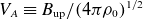
In figure 1(a), it can be seen that initially, close to
 $t=0$
,
$t=0$
,
 $\xi$
and
$\xi$
and
 $\eta$
evolve similarly for all values
$\eta$
evolve similarly for all values
 $R$
, with
$R$
, with
 $\xi$
displaying linear collapse and
$\xi$
displaying linear collapse and
 $\eta$
displaying linear growth. Additionally, it can be seen that irrespective of the strength of radiative cooling, there exists a finite-time singularity in the solution for
$\eta$
displaying linear growth. Additionally, it can be seen that irrespective of the strength of radiative cooling, there exists a finite-time singularity in the solution for
 $\xi$
. However, in the cases with stronger radiative cooling, it can be seen that the time at which
$\xi$
. However, in the cases with stronger radiative cooling, it can be seen that the time at which
 $\xi$
becomes singular, which we define as the critical time
$\xi$
becomes singular, which we define as the critical time
 $t_c$
, is reached earlier, implying that stronger cooling results in faster collapse of the X-point. Another particularly interesting feature that can be seen in the cases with stronger cooling, particularly
$t_c$
, is reached earlier, implying that stronger cooling results in faster collapse of the X-point. Another particularly interesting feature that can be seen in the cases with stronger cooling, particularly
 $R=300$
(black) and
$R=300$
(black) and
 $R=3000$
(yellow) is the presence of a turning point in the solution for
$R=3000$
(yellow) is the presence of a turning point in the solution for
 $\eta$
, implying that, for strong enough cooling, the outflows reverse before the X-point collapses entirely.
$\eta$
, implying that, for strong enough cooling, the outflows reverse before the X-point collapses entirely.
(a) Plot of
 $\xi$
(solid) and
$\xi$
(solid) and
 $\eta$
(dashed) vs time ‘t’ for Syrovatskii’s solution (
$\eta$
(dashed) vs time ‘t’ for Syrovatskii’s solution (
 $R=0$
, blue),
$R=0$
, blue),
 $R=3$
(weak cooling, green),
$R=3$
(weak cooling, green),
 $R=30$
(red),
$R=30$
(red),
 $R=300$
(black) and
$R=300$
(black) and
 $R=3000$
(strong cooling, yellow). It can be seen that stronger radiative cooling causes the X-point to collapse more rapidly in the inflow direction, and also potentially results in a reversal of the direction of the outflows. (b) Plot comparing the impact of non-uniform pressure without radiative cooling (blue) and with weak radiative cooling (
$R=3000$
(strong cooling, yellow). It can be seen that stronger radiative cooling causes the X-point to collapse more rapidly in the inflow direction, and also potentially results in a reversal of the direction of the outflows. (b) Plot comparing the impact of non-uniform pressure without radiative cooling (blue) and with weak radiative cooling (
 $R=3$
, pink) on
$R=3$
, pink) on
 $\xi$
(solid) and
$\xi$
(solid) and
 $\eta$
(dashed). For the same initial magnitude, the pressure modified by radiative cooling has a smaller
$\eta$
(dashed). For the same initial magnitude, the pressure modified by radiative cooling has a smaller
 $t_c$
; thus the effects observed in (a) can be attributed to radiative cooling, rather than just the non-uniform pressure.
$t_c$
; thus the effects observed in (a) can be attributed to radiative cooling, rather than just the non-uniform pressure.

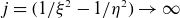
We can compare how the structure of the X-point is impacted by radiative cooling using two-dimensional contour plots of the magnetic flux function
 $\psi$
. In figure 2, we plot
$\psi$
. In figure 2, we plot
 $\psi (x,y)$
at
$\psi (x,y)$
at
 $t=0$
(a), and
$t=0$
(a), and
 $t=0.146$
for
$t=0.146$
for
 $R=0$
(b) and
$R=0$
(b) and
 $R=300$
(c). The time
$R=300$
(c). The time
 $t=0.146$
has been selected as it is close to
$t=0.146$
has been selected as it is close to
 $t_c$
for
$t_c$
for
 $R=300$
, showing a clear contrast between the radiatively cooled and non-radiative case. As expected, both the non-radiative and radiatively cooled cases have a narrower X-point along the inflow direction in comparison with the configuration without radiation (figure 2
a). However, the radiatively cooled X-point is significantly narrower that the non-radiative X-point at the same point in time; this is consistent with the results shown in figure 1(a), implying that radiative cooling results in faster collapse in the inflow direction. Additionally, it can also be seen that the radiatively cooled X-point is also collapsing along the outflow direction, unlike the non-radiative X-point, which continues to elongate; this is consistent with the flow reversal implied by the eventual decrease in
$R=300$
, showing a clear contrast between the radiatively cooled and non-radiative case. As expected, both the non-radiative and radiatively cooled cases have a narrower X-point along the inflow direction in comparison with the configuration without radiation (figure 2
a). However, the radiatively cooled X-point is significantly narrower that the non-radiative X-point at the same point in time; this is consistent with the results shown in figure 1(a), implying that radiative cooling results in faster collapse in the inflow direction. Additionally, it can also be seen that the radiatively cooled X-point is also collapsing along the outflow direction, unlike the non-radiative X-point, which continues to elongate; this is consistent with the flow reversal implied by the eventual decrease in
 $\eta (t)$
observed in figure 1(a).
$\eta (t)$
observed in figure 1(a).
Lastly, in figure 1(b), we compare the impacts of the simple non-uniform pressure term (blue) and the pressure term modified by radiative cooling (pink) on the evolution of
 $\xi$
and
$\xi$
and
 $\eta$
. A crucial difference in the physics in this paper compared with the derivation in S71 is the inclusion of non-uniform pressure; the derivation in S71 assumes the pressure to be uniform and thus not included in the dynamics of
$\eta$
. A crucial difference in the physics in this paper compared with the derivation in S71 is the inclusion of non-uniform pressure; the derivation in S71 assumes the pressure to be uniform and thus not included in the dynamics of
 $\xi$
and
$\xi$
and
 $\eta$
. As the solution that includes radiative cooling approaches the finite-time singularity earlier, the interesting behaviour of the solution for
$\eta$
. As the solution that includes radiative cooling approaches the finite-time singularity earlier, the interesting behaviour of the solution for
 $\eta$
as well as
$\eta$
as well as
 $t_c$
can primarily be attributed to radiative cooling.
$t_c$
can primarily be attributed to radiative cooling.
3.2. Asymptotic behaviour near finite-time singularity
The numerical solutions for both the case in S71 and the radiatively cooled case show the presence of a finite-time singularity at
 $t=t_c$
where
$t=t_c$
where
 $\xi =0$
. The behaviour
$\xi =0$
. The behaviour
 $\xi$
for
$\xi$
for
 $t\approx t_c$
can be analysed analytically as in this region;
$t\approx t_c$
can be analysed analytically as in this region;
 $1/\xi ^2$
is large and
$1/\xi ^2$
is large and
 $\eta \sim \eta (t_c)$
. This is done by Syrovatiskii in S71 (using (2.17)) to yield the scalings
$\eta \sim \eta (t_c)$
. This is done by Syrovatiskii in S71 (using (2.17)) to yield the scalings
 \begin{equation} \begin{aligned} & \xi \sim \left (t_c-t\right )^{2/3}, \eta \sim \eta \left (t_c\right ) \rightarrow \varGamma _x \sim -\left (t_c-t\right )^{-1}, \varGamma _y=\text{ constant } \\ & \Rightarrow \rho \sim \left (t_c-t\right )^{-2/3}, j \sim \left (t_c-t\right )^{-4/3}.\end{aligned} \end{equation}
Applying the same analysis for the radiatively cooled case is non-trivial as the treatment of the integral containing the radiative cooling term is not obvious. Thus, we consider the following two different limiting cases:
-
(i) small
 $R$
, weak radiative cooling: here, we can consider the radiative cooling term as a small correction to S71. The integral in this term can be evaluated using the non-radiative scaling
$\xi \sim (t_c-t)^{2/3}$
, allowing us to solve for
$\xi$
perturbatively; and
$R$
, weak radiative cooling: here, we can consider the radiative cooling term as a small correction to S71. The integral in this term can be evaluated using the non-radiative scaling
$\xi \sim (t_c-t)^{2/3}$
, allowing us to solve for
$\xi$
perturbatively; and -
(ii) large
$R$
, strong radiative cooling: here, we substitute the algebraically parameterised ansatz
$\sim (t_c-t)^{\alpha }$
into the equation for
$\xi$
and assume a dominant balance between
$\ddot {\xi }$
and the radiatively cooled term.


(a) Plot of the initial X-point configuration in terms of
 $\psi$
, where
$\psi$
, where
 $\xi =\xi _0=1$
and
$\xi =\xi _0=1$
and
 $\eta =\eta _0=1$
. Panels (b) and (c) plot the same set of contours of
$\eta =\eta _0=1$
. Panels (b) and (c) plot the same set of contours of
 $\psi$
as panel (a) with no radiative cooling (b) for
$\psi$
as panel (a) with no radiative cooling (b) for
 $t=0.146s$
, which is near the critical time
$t=0.146s$
, which is near the critical time
 $t_c=0.15s$
for the radiatively cooled case with
$t_c=0.15s$
for the radiatively cooled case with
 $R=300$
(c). It can be seen that, whilst both cases have a narrower X-point in the inflow direction, the radiatively cooled X-point is significantly narrower in the inflow direction and also appears to contract in the outflow direction, which is indicative of the flow reversal observed in figure 1.
$R=300$
(c). It can be seen that, whilst both cases have a narrower X-point in the inflow direction, the radiatively cooled X-point is significantly narrower in the inflow direction and also appears to contract in the outflow direction, which is indicative of the flow reversal observed in figure 1.

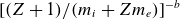
The dominant balances and methodology used for each case are confirmed using the plots in figure 3, which compares the size of each term in the equation for
 $\ddot {\xi }$
in (2.31).
$\ddot {\xi }$
in (2.31).
(a) Plot of each term in the equation for
 $\ddot {\xi }$
(2.28) for
$\ddot {\xi }$
(2.28) for
 $R=3$
(weak cooling) up to
$R=3$
(weak cooling) up to
 $t=t_c$
. It can be seen that, whilst
$t=t_c$
. It can be seen that, whilst
 $1/\xi ^2$
(blue) is the dominant term, there is a small contribution from radiative cooling (red). (b) Plot for
$1/\xi ^2$
(blue) is the dominant term, there is a small contribution from radiative cooling (red). (b) Plot for
 $R=300$
(strong cooling) up to
$R=300$
(strong cooling) up to
 $t=t_c$
, clearly showing radiative cooling (red) to be the dominant term. In both plots, it can be seen that the contribution of
$t=t_c$
, clearly showing radiative cooling (red) to be the dominant term. In both plots, it can be seen that the contribution of
 $1/\eta ^2$
(green) is negligible, whilst the albeit more significant contribution of the
$1/\eta ^2$
(green) is negligible, whilst the albeit more significant contribution of the
 $1/J^{\gamma }$
term (non-uniform pressure, yellow) can be neglected near
$1/J^{\gamma }$
term (non-uniform pressure, yellow) can be neglected near
 $t=t_c$
.
$t=t_c$
.

3.2.1. Weak cooling: small
$R$
corrections

First we consider the case with small
 $R$
; as before, near
$R$
; as before, near
 $t\approx t_c$
,
$t\approx t_c$
,
 $1/\xi ^2\gg 1/\eta ^2$
, allowing us to neglect the
$1/\xi ^2\gg 1/\eta ^2$
, allowing us to neglect the
 $1/\eta ^2$
term. Additionally, as
$1/\eta ^2$
term. Additionally, as
 $\eta \approx \eta (t_c)\gg \xi$
, we also consider the
$\eta \approx \eta (t_c)\gg \xi$
, we also consider the
 $1/(\xi \eta ^{\gamma })$
term to be negligible given that
$1/(\xi \eta ^{\gamma })$
term to be negligible given that
 $\gamma =5/3\lt 2 \to 1/\xi ^2\gg 1/(\eta (t_c)\xi )^{5/3}$
. Substituting
$\gamma =5/3\lt 2 \to 1/\xi ^2\gg 1/(\eta (t_c)\xi )^{5/3}$
. Substituting
 $\xi \sim (t_c-t)^{2/3}$
and
$\xi \sim (t_c-t)^{2/3}$
and
 $\eta \approx \eta (t_c)$
into
$\eta \approx \eta (t_c)$
into
 $I[\xi \eta ]$
thus gives the following expression for
$I[\xi \eta ]$
thus gives the following expression for
 $\ddot {\xi }$
:
$\ddot {\xi }$
:
 \begin{equation} \ddot {\xi } \approx -\eta \left (t_c\right )\left [\frac {1}{\xi ^2}+C_{\text{int}}(t_c-t)^{2\alpha _p/3+(1/(1-b))}\right ] \quad \text{and} \quad \alpha _p=\frac {b-a}{(1-b)}, \end{equation}
where
 \begin{equation} C_{\text{int}}=\widetilde {C}_{\text{cool}} \left [\frac {9}{2} \eta (t_c)^4\right ]^{(b-a)/ 3(1-b)}\left [\frac {3}{2[b(1-\gamma )+(\gamma -a)]+3}\right ]^{1/(1-b)}. \end{equation}
For bremsstrahlung cooling, with
 $a=2,b=1/2$
and
$a=2,b=1/2$
and
 $\gamma =5/3$
, this equation becomes
$\gamma =5/3$
, this equation becomes
 \begin{equation} \ddot {\xi } \approx -\eta (t_c)\left (\frac {1}{\xi ^2}+C_{\text{int}}\right ). \end{equation}
Using the following labeling of constants:
 \begin{align} & c_1=-\eta (t_c), \nonumber\\[3pt] & c_2=-C_{\text{int}} \eta (t_c), \nonumber\\[3pt] & c_3=\frac {c_1^{-1 / 3}/2-c_2c_1^{2 / 3}}{c_1^{1 / 3}}, \nonumber\\[3pt] &\xi (t=t_c)=0, \end{align}
the general solution to this equation (solved in Appendix B) can be written as
 \begin{equation} (t_c-t)=\int ^{\xi (t_c)}_{\xi _0} \sqrt {\frac {\xi }{\big(2 c_3 c_1^{2 / 3} \xi +2 c_2 \xi ^2-2 c_1\big)}} {\rm d} \xi . \end{equation}
For small
 $\xi$
, the integrand is
$\xi$
, the integrand is
 $\sim O(\xi ^{1/2})$
and thus the dominant contribution of this integral comes from the region where
$\sim O(\xi ^{1/2})$
and thus the dominant contribution of this integral comes from the region where
 $t\approx t_c$
, to yield
$t\approx t_c$
, to yield
 \begin{equation} \left (t_c-t\right )=\frac {2}{3} \sqrt {-\frac {1}{c_1}} \xi ^{3 / 2}-\frac {2}{5}\left [c_3 c_1^{2/3}\left (-\frac {1}{c_1}\right )^{3/2}\right ]\xi ^{5/2}+O(\xi ^{7/2}). \end{equation}
To lowest order, this retrieves the S71 scaling of
 $\xi \sim (t_c-t)^{2/3}$
. When plugging in this scaling with a corrective term to
$\xi \sim (t_c-t)^{2/3}$
. When plugging in this scaling with a corrective term to
 $\sim O(\xi ^{5/2})$
, we find a correction term which scales as
$\sim O(\xi ^{5/2})$
, we find a correction term which scales as
 $\sim (t_c-t)^{4/3}$
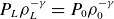
. This scaling (see Appendix B for the full expression) is a good fit for the data, as shown in figure 4(a), where the curve representing this scaling (blue) converges to the data (green) as
$\sim (t_c-t)^{4/3}$
. This scaling (see Appendix B for the full expression) is a good fit for the data, as shown in figure 4(a), where the curve representing this scaling (blue) converges to the data (green) as
 $t$
approaches
$t$
approaches
 $t_c$
.
$t_c$
.
3.2.2. Strong cooling: algebraic parameterisation
Now, the case where
 $R$
is large can be analysed by parameterising
$R$
is large can be analysed by parameterising
 $\xi$
near
$\xi$
near
 $t_c$
as
$t_c$
as
 $\sim (t_c-t)^{\alpha }$
and solving for
$\sim (t_c-t)^{\alpha }$
and solving for
 $\alpha$
in the equation for
$\alpha$
in the equation for
 $\ddot {\xi }$
(2.31) by considering the appropriate dominant balances
$\ddot {\xi }$
(2.31) by considering the appropriate dominant balances
 \begin{align}& \ddot {\xi } \approx - \eta \left (t_c\right )\left [\left (t_c-t\right )^{-2 \alpha }+\frac {C_{\text{int}}\left (t_c-t\right )^{({\alpha [b(1-\gamma )+(\gamma -a)]+1)}/{(1-b)}}}{\eta \left (t_c\right )^\gamma \left (t_c-t\right )^{\alpha \gamma }}\right ],\\[-10pt]\nonumber \end{align}
 \begin{align}& (t_c-t)^{\alpha -2}\approx \eta \left (t_c\right )\left [\left (t_c-t\right )^{-2 \alpha }+\frac {C_{\text{int}}\left (t_c-t\right )^{{(\alpha (b-a)+1)}/{(1-b)}}}{\eta \left (t_c\right )^\gamma }\right ]. \end{align}
There are two reasonable dominant balances here based on the regime. First, with no radiative cooling, the dominant balance is
 \begin{equation} (t_c-t)^{\alpha -2}\sim (t_c-t)^{-2\alpha } \to \alpha =\frac {2}{3}, \end{equation}
which returns the scaling in S71, as expected. The other dominant balance, which is evident for a sufficiently large
 $R$
, as seen in figure 3(b), is
$R$
, as seen in figure 3(b), is
 \begin{align} \ddot {\xi } & \sim \frac {C_{\text{int}}\left (t_c-t\right )^{({\alpha (b-a)+1)}/{(1-b)}}}{\eta \left (t_c\right )^\gamma } \to (t_c-t)^{\alpha -2}\nonumber\\&\sim (t_c-t)^{{(\alpha (b-a)+1)}/{(1-b)}} \to \alpha \approx \left [\frac {3-2b}{1-2b+a}\right ]. \end{align}
For bremsstrahlung cooling, this gives
 $\alpha \approx 1$
, yielding
$\alpha \approx 1$
, yielding
 \begin{equation} \xi \sim (t_c-t), \eta \approx \eta (t_c) . \end{equation}
Here, we still assume that
 $\eta \ll \xi$
near
$\eta \ll \xi$
near
 $t=t_c$
; although technically there is a large enough value of
$t=t_c$
; although technically there is a large enough value of
 $R$
such that
$R$
such that
 $\xi \sim \eta$
. However, we are not aware of any astrophysical environment where such a large value of
$\xi \sim \eta$
. However, we are not aware of any astrophysical environment where such a large value of
 $R$
would be relevant. Similar to the scaling for small
$R$
would be relevant. Similar to the scaling for small
 $R$
, this scaling is shown to be a good fit for the data, in figure 4(b).
$R$
, this scaling is shown to be a good fit for the data, in figure 4(b).
Given the results obtained for weak cooling from (3.7) and strong cooling in (3.12), it can be seen that radiative cooling accelerates the collapse of
 $\xi$
near
$\xi$
near
 $t\approx t_c$
, with stronger cooling resulting in more rapid collapse.
$t\approx t_c$
, with stronger cooling resulting in more rapid collapse.
Plots comparing the derived scalings near the finite-time singularity (blue) with the numerical solution for
 $\xi$
(green) for
$\xi$
(green) for
 $R=3$
(a, weak cooling) and
$R=3$
(a, weak cooling) and
 $R=300$
(b, strong cooling). Here, the range in
$R=300$
(b, strong cooling). Here, the range in
 $t$
has been selected to highlight behaviour near
$t$
has been selected to highlight behaviour near
 $t\approx t_c$
.
$t\approx t_c$
.

3.3. Force balance and critical
$R$

A particularly prominent feature in the solutions for
 $\xi$
and
$\xi$
and
 $\eta$
in figure 1(a) is the presence of a turning point in
$\eta$
in figure 1(a) is the presence of a turning point in
 $\eta$
, implying the reversal of the outflows in the presence of strong radiative cooling (higher values of
$\eta$
, implying the reversal of the outflows in the presence of strong radiative cooling (higher values of
 $R$
). Given this result, we would like to understand what is the underlying physical mechanism that dictates such reversal, and what is the critical value of
$R$
). Given this result, we would like to understand what is the underlying physical mechanism that dictates such reversal, and what is the critical value of
 $\widetilde {C}_{\text{cool}}$
, and thus
$\widetilde {C}_{\text{cool}}$
, and thus
 $R$
, above which this occurs.
$R$
, above which this occurs.
The underlying physical mechanism dictating this reversal of flows can be qualitatively understood by separately considering the pressure imbalance due to radiative cooling and the subsequent response along the
 $x$
-axis and the
$x$
-axis and the
 $y$
-axis. Starting with the initial configuration of dominant forces due to pressure gradients; along the
$y$
-axis. Starting with the initial configuration of dominant forces due to pressure gradients; along the
 $y$
-axis (outflow direction), the force on a plasma parcel due to both the thermal pressure gradient and the
$y$
-axis (outflow direction), the force on a plasma parcel due to both the thermal pressure gradient and the
 $\boldsymbol{j}\times \boldsymbol{B}$
force point in the direction of the outflows, yielding a positive kinetic pressure gradient. This is because the thermal pressure profile is parabolic with its maximum at the X-point, and the outflow velocity is positive (
$\boldsymbol{j}\times \boldsymbol{B}$
force point in the direction of the outflows, yielding a positive kinetic pressure gradient. This is because the thermal pressure profile is parabolic with its maximum at the X-point, and the outflow velocity is positive (
 $\varGamma _{y,0}\gt 0$
). Along the
$\varGamma _{y,0}\gt 0$
). Along the
 $x$
-axis, the force on the plasma parcel due to the magnetic pressure gradient points in the direction of the inflows and is opposed by the force due to the thermal pressure gradient. Dynamically, radiative cooling (which is stronger at
$x$
-axis, the force on the plasma parcel due to the magnetic pressure gradient points in the direction of the inflows and is opposed by the force due to the thermal pressure gradient. Dynamically, radiative cooling (which is stronger at
 $y_0=0$
due to the parabolic pressure profile) results in a drop in temperature and thus thermal pressure. This results in an instantaneous increase in pressure imbalance in the
$y_0=0$
due to the parabolic pressure profile) results in a drop in temperature and thus thermal pressure. This results in an instantaneous increase in pressure imbalance in the
 $x$
-direction, resulting in the compression of the plasma and subsequent increase in density by the magnetic pressure. Whilst both thermal pressure and the radiative cooling power density
$x$
-direction, resulting in the compression of the plasma and subsequent increase in density by the magnetic pressure. Whilst both thermal pressure and the radiative cooling power density
 $\dot {Q} \sim \rho ^aT^b$
increase with an increase in density, cooling mechanisms with
$\dot {Q} \sim \rho ^aT^b$
increase with an increase in density, cooling mechanisms with
 $a\gt 1$
will result in an additional drop in thermal pressure. Notably, this runaway drop in thermal pressure is expected to be more significant at the X-point as the radiative cooling is stronger at
$a\gt 1$
will result in an additional drop in thermal pressure. Notably, this runaway drop in thermal pressure is expected to be more significant at the X-point as the radiative cooling is stronger at
 $(x_0, y_0)=(0,0)$
due to the parabolic pressure profile, resulting in stronger compression at the X-point by the magnetic pressure. As a result, the thermal pressure at the X-point will eventually fall below that of the surrounding plasma, reversing the direction of the thermal pressure gradient. The force induced due to this therefore opposes
$(x_0, y_0)=(0,0)$
due to the parabolic pressure profile, resulting in stronger compression at the X-point by the magnetic pressure. As a result, the thermal pressure at the X-point will eventually fall below that of the surrounding plasma, reversing the direction of the thermal pressure gradient. The force induced due to this therefore opposes
 $\boldsymbol{j}\times \boldsymbol{B}$
force that drives the kinetic pressure gradient of the outflows. For strong enough cooling (large enough
$\boldsymbol{j}\times \boldsymbol{B}$
force that drives the kinetic pressure gradient of the outflows. For strong enough cooling (large enough
 $R$
), this inward pointing thermal pressure gradient can become large enough to not only balance but dominate the opposing forces, consequently stalling and reversing the direction of the outflows.
$R$
), this inward pointing thermal pressure gradient can become large enough to not only balance but dominate the opposing forces, consequently stalling and reversing the direction of the outflows.
We choose to define the critical
 $R\equiv R^{\star }$
to be the value of
$R\equiv R^{\star }$
to be the value of
 $R$
at which the cooling term is of the same order as
$R$
at which the cooling term is of the same order as
 $1/\xi ^2$
near the finite-time singularity; this implies that the cooling term at the very least balances other terms at its maximum, which it reaches at
$1/\xi ^2$
near the finite-time singularity; this implies that the cooling term at the very least balances other terms at its maximum, which it reaches at
 $t=t_c$
. With the natural assumption that the observed impact on
$t=t_c$
. With the natural assumption that the observed impact on
 $\eta$
can be attributed to radiative cooling, we would expect radiative cooling mechanisms with values of
$\eta$
can be attributed to radiative cooling, we would expect radiative cooling mechanisms with values of
 $R$
distinctly greater than
$R$
distinctly greater than
 $R^{\star }$
to result in the deceleration and reversal of the outflows.
$R^{\star }$
to result in the deceleration and reversal of the outflows.
From the analysis of the behaviour of
 $\xi$
near the finite-time singularity and the results in figure 1(a),
$\xi$
near the finite-time singularity and the results in figure 1(a),
 $R^{\star }$
likely inhabits an intermediate cooling regime, for which the behaviour of
$R^{\star }$
likely inhabits an intermediate cooling regime, for which the behaviour of
 $\xi (t)$
near
$\xi (t)$
near
 $t_c$
is unknown. However, it can be assumed that for such a regime, the following terms in the equation for
$t_c$
is unknown. However, it can be assumed that for such a regime, the following terms in the equation for
 $\ddot {\xi }$
(2.31) balance:
$\ddot {\xi }$
(2.31) balance:
 \begin{equation} \frac {\ddot {\xi }}{\eta (t_c)} \sim \frac {1}{\xi ^2}\sim \frac {\widetilde {C}_{\text{cool}} I[\xi \eta (t_c)]^{1/(1-b)}}{\eta (t_c)^{\gamma }\xi ^\gamma }, \end{equation}
and thus have the same time dependence near
 $t_c$
, with an integration constant of order unity. It can be noted that as there is no expected turning point in
$t_c$
, with an integration constant of order unity. It can be noted that as there is no expected turning point in
 $\eta$
for
$\eta$
for
 $t\ll t_c$
in this intermediate regime,
$t\ll t_c$
in this intermediate regime,
 $\xi \ll \eta$
, allowing us to neglect the
$\xi \ll \eta$
, allowing us to neglect the
 $1/(\xi \eta )^{\gamma }$
and
$1/(\xi \eta )^{\gamma }$
and
 $1/\eta ^2$
terms. Thus, considering the average value of
$1/\eta ^2$
terms. Thus, considering the average value of
 $\eta (t_c)$
at that point (see figure 1) along with the integration constants for bremsstrahlung cooling,
$\eta (t_c)$
at that point (see figure 1) along with the integration constants for bremsstrahlung cooling,
 $\widetilde {C}_{\text{cool}}^{\star }$
can be estimated from (3.13) to be
$\widetilde {C}_{\text{cool}}^{\star }$
can be estimated from (3.13) to be
 $\widetilde {C}_{\text{cool}}^{\star } \approx 10$
, with a corresponding
$\widetilde {C}_{\text{cool}}^{\star } \approx 10$
, with a corresponding
 $R^{\star }\approx 10$
.
$R^{\star }\approx 10$
.
(a) Plot of
 $\xi$
(solid) and
$\xi$
(solid) and
 $\eta$
(dashed) vs time
$\eta$
(dashed) vs time
 $t$
for
$t$
for
 $R=3$
(green),
$R=3$
(green),
 $R=10 \approx R^{\star }$
(red),
$R=10 \approx R^{\star }$
(red),
 $R=16$
(blue) and
$R=16$
(blue) and
 $R=30$
(black). (b) Plot of
$R=30$
(black). (b) Plot of
 $\xi$
(solid) and
$\xi$
(solid) and
 $\dot {\eta }$
(dashed) vs time
$\dot {\eta }$
(dashed) vs time
 $t/\tau _{A}$
for
$t/\tau _{A}$
for
 $R=3$
(green),
$R=3$
(green),
 $R=10 \approx R^{\star }$
(red),
$R=10 \approx R^{\star }$
(red),
 $R=16$
(blue) and
$R=16$
(blue) and
 $R=30$
(black) to show that, for
$R=30$
(black) to show that, for
 $R\geqslant R^{\star }$
, the outflows decelerate (
$R\geqslant R^{\star }$
, the outflows decelerate (
 $\dot {\eta }\lt \eta _0$
) and for a high enough
$\dot {\eta }\lt \eta _0$
) and for a high enough
 $R=30$
, the outflows halt (
$R=30$
, the outflows halt (
 $\dot {\eta }=0$
).
$\dot {\eta }=0$
).

The impact of these predicted values can clearly be seen in figures 5(a) and 5(b), which plot
 $\xi$
along with
$\xi$
along with
 $\eta$
(a) and
$\eta$
(a) and
 $\dot {\eta }$
(b) over time for
$\dot {\eta }$
(b) over time for
 $R=3$
, (green),
$R=3$
, (green),
 $R=10 \approx R^{\star }$
(red),
$R=10 \approx R^{\star }$
(red),
 $R= 16$
(blue) and
$R= 16$
(blue) and
 $R=30$
(black) for bremsstrahlung cooling. In figure 5, it can be seen that the evolution of
$R=30$
(black) for bremsstrahlung cooling. In figure 5, it can be seen that the evolution of
 $\eta$
for
$\eta$
for
 $R=10 \approx R^{\star }$
(red) begins to deviate from the weak cooling case (
$R=10 \approx R^{\star }$
(red) begins to deviate from the weak cooling case (
 $R=3$
, green), whilst for
$R=3$
, green), whilst for
 $R=30$
(black),
$R=30$
(black),
 $\eta$
begins to collapse at
$\eta$
begins to collapse at
 $t\lt t_c$
. In figure 5(b), the impact of cooling on the outflows can be seen more clearly. For weak cooling (
$t\lt t_c$
. In figure 5(b), the impact of cooling on the outflows can be seen more clearly. For weak cooling (
 $R=3)$
,
$R=3)$
,
 $\dot {\eta }$
always has a positive slope, however, in contrast, for
$\dot {\eta }$
always has a positive slope, however, in contrast, for
 $R\gtrsim 10 \approx R^{\star }$
,
$R\gtrsim 10 \approx R^{\star }$
,
 $\dot {\eta }$
has some negative slope, indicating the deceleration of the outflows. Crucially, for
$\dot {\eta }$
has some negative slope, indicating the deceleration of the outflows. Crucially, for
 $R=30$
, which is the first value of
$R=30$
, which is the first value of
 $R$
that is distinctly greater than
$R$
that is distinctly greater than
 $R^{\star }$
, the outflows are shown to not just decelerate, but to halt (
$R^{\star }$
, the outflows are shown to not just decelerate, but to halt (
 $\dot {\eta }=0$
) before
$\dot {\eta }=0$
) before
 $t_c$
and reverse in direction (
$t_c$
and reverse in direction (
 $\dot {\eta }\lt 0$
).
$\dot {\eta }\lt 0$
).
4. Modified Sweet–Parker model
In reality, there will be mechanisms that stop the rapid collapse by heating the plasma and counteracting the strong inward thermal pressure gradient. Beyond compressional heating, a candidate for this is ohmic heating. The volumetric ohmic heating rate
 $\int \dot {Q}_{\varOmega }\, \text{d}V$
, where
$\int \dot {Q}_{\varOmega }\, \text{d}V$
, where
 $V$
is taken to be the volume of the current sheet and
$V$
is taken to be the volume of the current sheet and
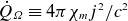 $\dot {Q}_{\varOmega }\equiv 4\pi \chi _mj^2/c^2$
, is deemed to be negligible as the magnetic diffusivity
$\dot {Q}_{\varOmega }\equiv 4\pi \chi _mj^2/c^2$
, is deemed to be negligible as the magnetic diffusivity
 $\chi _m$
is small; however, close to
$\chi _m$
is small; however, close to
 $t_c$
, the gradients in
$t_c$
, the gradients in
 $B$
are strong enough to generate a large enough current
$B$
are strong enough to generate a large enough current
 $j$
such that
$j$
such that
 $\dot {Q}_{\varOmega }$
can no longer be neglected. This can be seen by evaluating the approximate time at which the resistive diffusion rate
$\dot {Q}_{\varOmega }$
can no longer be neglected. This can be seen by evaluating the approximate time at which the resistive diffusion rate
 $\tau _{\chi _m}^{-1}\sim \chi _m/\xi ^2$
and the X-point collapse rate along the
$\tau _{\chi _m}^{-1}\sim \chi _m/\xi ^2$
and the X-point collapse rate along the
 $x$
-axis
$x$
-axis
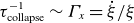 $\tau _{\text{collapse}}^{-1}\sim \varGamma _x=\dot {\xi }/\xi$
balance. Using the asymptotic expressions derived for
$\tau _{\text{collapse}}^{-1}\sim \varGamma _x=\dot {\xi }/\xi$
balance. Using the asymptotic expressions derived for
 $\xi$
in (3.1) and (3.12), these terms balance at some time
$\xi$
in (3.1) and (3.12), these terms balance at some time
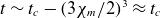 $t\sim t_c - (3\chi _m/2)^3\approx t_c$
for the case without cooling and
$t\sim t_c - (3\chi _m/2)^3\approx t_c$
for the case without cooling and
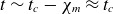 $t\sim t_c -\chi _m \approx t_c$
with strong radiative cooling. Given this result, it is worth considering what a steady-state solution looks like, if one should exist. This can be achieved by expanding on the radiatively cooled Sweet–Parker model developed by Uzdensky & McKinney (Reference Uzdensky and McKinney2011) to include the length of the current sheet as a variable, as our current sheet model predicts that, for strong enough cooling, the current sheet will have already started contracting before a steady state is achieved.
$t\sim t_c -\chi _m \approx t_c$
with strong radiative cooling. Given this result, it is worth considering what a steady-state solution looks like, if one should exist. This can be achieved by expanding on the radiatively cooled Sweet–Parker model developed by Uzdensky & McKinney (Reference Uzdensky and McKinney2011) to include the length of the current sheet as a variable, as our current sheet model predicts that, for strong enough cooling, the current sheet will have already started contracting before a steady state is achieved.
For a current sheet of length
 $2L$
and width
$2L$
and width
 $2\delta$
such that
$2\delta$
such that
 $\delta \ll L$
(this remains true even if the current sheet contracts, see figure 1), we define the upstream magnetic field, velocity, mass density and number density to be
$\delta \ll L$
(this remains true even if the current sheet contracts, see figure 1), we define the upstream magnetic field, velocity, mass density and number density to be
 $B_{\text{in}}$
,
$B_{\text{in}}$
,
 $v_{\text{in}}$
,
$v_{\text{in}}$
,
 $\rho _{\text{in}}$
and
$\rho _{\text{in}}$
and
 $n_{\text{in}}$
, respectively. Similarly, we label the corresponding downstream magnetic field, velocity, mass density and number density to be
$n_{\text{in}}$
, respectively. Similarly, we label the corresponding downstream magnetic field, velocity, mass density and number density to be
 $B_{\text{out}}$
,
$B_{\text{out}}$
,
 $v_{\text{out}}$
,
$v_{\text{out}}$
,
 $\rho _{\text{out}}$
and
$\rho _{\text{out}}$
and
 $n_{\text{out}}$
. In contrast to the standard, incompressible Sweet–Parker model, there are two additional variables here:
$n_{\text{out}}$
. In contrast to the standard, incompressible Sweet–Parker model, there are two additional variables here:
 $n_{\text{out}}$
(or
$n_{\text{out}}$
(or
 $\rho _{\text{out}}$
) due to the inclusion of plasma compressibility, and
$\rho _{\text{out}}$
) due to the inclusion of plasma compressibility, and
 $L$
. The equations are closed by Uzdensky & McKinney (Reference Uzdensky and McKinney2011) to find
$L$
. The equations are closed by Uzdensky & McKinney (Reference Uzdensky and McKinney2011) to find
 $n_{\text{out}}$
by assuming volumetric power balance between ohmic heating (which we approximate to be held locally)
$n_{\text{out}}$
by assuming volumetric power balance between ohmic heating (which we approximate to be held locally)
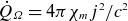 $\dot {Q}_{\varOmega }=4\pi \chi _mj^2/c^2$
and radiative cooling
$\dot {Q}_{\varOmega }=4\pi \chi _mj^2/c^2$
and radiative cooling
 $\dot {Q}_{\text{rad}}=C_{\text{cool}}\rho ^aT^b$
. To close the equations with varying
$\dot {Q}_{\text{rad}}=C_{\text{cool}}\rho ^aT^b$
. To close the equations with varying
 $L$
, we further assume that this steady state is achieved if the advection time
$L$
, we further assume that this steady state is achieved if the advection time
 $\tau _A$
is similar to the cooling time
$\tau _A$
is similar to the cooling time
 $\tau _{\text{cool}}$
, allowing the reconnection process to occur before a given plasma parcel in the layer can radiatively collapse.
$\tau _{\text{cool}}$
, allowing the reconnection process to occur before a given plasma parcel in the layer can radiatively collapse.
Starting with the MHD continuity equation, allowing for compressibility results in
 \begin{equation} \rho _{\text{in}} {v_{\text{in}}} L \sim \rho _{\text{out}} v_{\text{out}} \delta \to {v_{\text{in}}} L \sim A v_{\text{out}} \delta , \end{equation}
where we define the compression ratio
 $A\equiv \rho _X/\rho _{\text{in}}$
. Here, for simplicity, we assume that the steady state has no significant variation in density along the layer such that
$A\equiv \rho _X/\rho _{\text{in}}$
. Here, for simplicity, we assume that the steady state has no significant variation in density along the layer such that
 $\rho _X\approx \rho _{\text{out}}$
and
$\rho _X\approx \rho _{\text{out}}$
and
 $A\approx \rho _{\text{out}}/\rho _{\text{in}}$
; this was also assumed in the calculation performed by Uzdensky & McKinney (Reference Uzdensky and McKinney2011) and is justified by the presence of radiative cooling. Similar to the incompressible Sweet–Parker model, the steady-state assumption enforced via Ohm’s law yields
$A\approx \rho _{\text{out}}/\rho _{\text{in}}$
; this was also assumed in the calculation performed by Uzdensky & McKinney (Reference Uzdensky and McKinney2011) and is justified by the presence of radiative cooling. Similar to the incompressible Sweet–Parker model, the steady-state assumption enforced via Ohm’s law yields
 ${v_{\text{in}}} \sim \chi _m/\delta$
. Additionally, the outflow component of the momentum equation can be used to find the outflow velocity
${v_{\text{in}}} \sim \chi _m/\delta$
. Additionally, the outflow component of the momentum equation can be used to find the outflow velocity
 \begin{equation} \frac {\rho _{\text{out}} v_{\text{out}}^2}{2} \sim P_{\text{in}} -P_{\textrm {out}} + \frac {B_{\text{in}}^2}{8\pi } + \frac {B_{\text{in}}^2}{4\pi } A, \end{equation}
where we have substituted
 $P_X$
using the pressure balance condition in the inflow direction
$P_X$
using the pressure balance condition in the inflow direction
 $P_X=P_{\text{in}}+B_{\text{in}}^2/8\pi$
. We assume, as usual, that
$P_X=P_{\text{in}}+B_{\text{in}}^2/8\pi$
. We assume, as usual, that
 $P_{\text{in}}\approx P_{\textrm {out}}$
, implying
$P_{\text{in}}\approx P_{\textrm {out}}$
, implying
 $T_{\textrm {in}}\gt T_{\textrm {out}}$
for
$T_{\textrm {in}}\gt T_{\textrm {out}}$
for
 $A\gt 1$
, which is consistent with the radiative cooling of the current sheet.Footnote
4
This then yields
$A\gt 1$
, which is consistent with the radiative cooling of the current sheet.Footnote
4
This then yields
 \begin{equation} v_{\text{out}}\approx V_A\left (\frac {1+2A}{A}\right )^{1/2}, \end{equation}
where the factor
 $(1+2A)^{1/2}/A^{1/2}$
can be shown to be of order unity (which we ignore for the purpose of this calculation) by considering the limits of
$(1+2A)^{1/2}/A^{1/2}$
can be shown to be of order unity (which we ignore for the purpose of this calculation) by considering the limits of
 $A$
; for
$A$
; for
 $A\sim \mathcal{O}(1)$
,
$A\sim \mathcal{O}(1)$
,
 $v_{\text{out}}\approx \sqrt {3}V_A$
and for
$v_{\text{out}}\approx \sqrt {3}V_A$
and for
 $A\gg 1$
,
$A\gg 1$
,
 $v_{\text{out}}\approx \sqrt {2}V_A$
.Footnote
5
$v_{\text{out}}\approx \sqrt {2}V_A$
.Footnote
5
Combining the expressions above, the following expression for the reconnection rate can be obtained:
 \begin{equation} \frac {{v_{\text{in}}}}{V_A}\sim A^{1/2}S_L^{-1/2}, \end{equation}
where
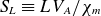 $S_L\equiv LV_A/\chi _m$
is the Lundquist number for a reconnection layer of length
$S_L\equiv LV_A/\chi _m$
is the Lundquist number for a reconnection layer of length
 $L$
. Thus, in order to make a definitive comparison between this expression and the expected incompressible Sweet–Parker reconnection rate in the absence of radiative cooling, explicit expressions for
$L$
. Thus, in order to make a definitive comparison between this expression and the expected incompressible Sweet–Parker reconnection rate in the absence of radiative cooling, explicit expressions for
 $A$
and
$A$
and
 $L$
need to be obtained by enforcing
$L$
need to be obtained by enforcing
 $\dot {Q}_{\varOmega }=\dot {Q}_{\text{rad}}$
and
$\dot {Q}_{\varOmega }=\dot {Q}_{\text{rad}}$
and
 $\tau _{\text{cool}}=\tau _A$
.
$\tau _{\text{cool}}=\tau _A$
.
Starting with the power balance condition, which we approximate as
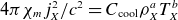 $4\pi \chi _mj_X^2/c^2=C_{\text{cool}}\rho _X^aT_X^b$
, where the subscript ‘
$4\pi \chi _mj_X^2/c^2=C_{\text{cool}}\rho _X^aT_X^b$
, where the subscript ‘
 $X$
’ denotes quantities measured at the X-point, we have
$X$
’ denotes quantities measured at the X-point, we have
 \begin{equation} \chi _m\frac {B_{\text{in}}^2}{4\pi \delta ^2}\sim \frac {\overline {C}_{\text{cool}}}{\gamma -1}\rho _X^{a-b}P_X^b . \end{equation}
Here,
 $P_X$
can be conveniently re-expressed in terms of
$P_X$
can be conveniently re-expressed in terms of
 $B_{\text{in}}$
using the required pressure balance in the inflow direction
$B_{\text{in}}$
using the required pressure balance in the inflow direction
 $P_X=P_{\text{in}}+B_{\text{in}}^2/8\pi =(1+\beta _{\text{in}})B_{\text{in}}^2/8\pi$
, where
$P_X=P_{\text{in}}+B_{\text{in}}^2/8\pi =(1+\beta _{\text{in}})B_{\text{in}}^2/8\pi$
, where
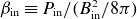 $\beta _{\text{in}}\equiv P_{\text{in}}/(B_{\text{in}}^2/8\pi )$
is the inflow plasma beta. It is also convenient to define
$\beta _{\text{in}}\equiv P_{\text{in}}/(B_{\text{in}}^2/8\pi )$
is the inflow plasma beta. It is also convenient to define
 $\mathcal{R}$
(2.37) for the inflows
$\mathcal{R}$
(2.37) for the inflows
 \begin{equation} \mathcal{R}=\frac {\overline {C}_{\text{cool}}\rho _{\text{in}}^{a-b}P_{\text{in}}^b}{\gamma P_{\text{in}} c_s/L_{\text{sys}}}\approx \frac {\overline {C}_{\text{cool}}\rho _{\text{in}}^{a-b}P_{\text{in}}^{b-1}L_{\text{sys}}}{\gamma ^{3/2}\beta _{\text{in}}^{1/2}V_A}, \end{equation}
where the sound speed is now defined in terms of inflow quantities
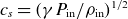 $c_s=(\gamma P_{\text{in}}/\rho _{\text{in}})^{1/2}$
and
$c_s=(\gamma P_{\text{in}}/\rho _{\text{in}})^{1/2}$
and
 $L_{\text{sys}}$
is the characteristic system size. Note that this is expressed entirely in terms of quantities assumed to be known. We are specifically interested in cases where
$L_{\text{sys}}$
is the characteristic system size. Note that this is expressed entirely in terms of quantities assumed to be known. We are specifically interested in cases where
 $\mathcal{R}\gg 1$
.
$\mathcal{R}\gg 1$
.
Plugging these expressions into (4.5) yields
 \begin{equation} \frac {L}{L_{\text{sys}}}\sim \frac {(\gamma -1)}{\mathcal{R}\gamma ^{3/2}}\frac {\beta _{\text{in}}^{b-3/2}}{(1+\beta _{\text{in}})^b}A^{b-a+1}. \end{equation}
Next, enforcing
 $\tau _{\text{cool}}=\tau _A$
implies
$\tau _{\text{cool}}=\tau _A$
implies
 \begin{equation} \frac {L}{V_A}=\frac {P_X}{C_{\text{cool}}\rho _X^aT_X^b}=\frac {(\gamma -1)}{\overline {C}_{\text{cool}}}P_X^{1-b}\rho _X^{b-a}, \end{equation}
which consequently yields the following expression for
 $L/L_{\text{sys}}$
in terms of
$L/L_{\text{sys}}$
in terms of
 $A$
,
$A$
,
 $\mathcal{R}$
and
$\mathcal{R}$
and
 $\beta _{\text{in}}$
:
$\beta _{\text{in}}$
:
 \begin{equation} \frac {L}{L_{\text{sys}}}\sim \frac {(\gamma -1)}{\mathcal{R}\gamma ^{3/2}}\frac {\beta _{\text{in}}^{b-3/2}}{(1+\beta _{\text{in}})^{b-1}}A^{b-a} . \end{equation}
Finally, equating the right-hand sides of (4.7) and (4.9) results in the following explicit expression for
 $A$
:
$A$
:
 \begin{equation} A\approx 1+\beta _{\text{in}}. \end{equation}
This expression is notably independent of the cooling mechanism (at least as long as the radiative power loss due to the cooling mechanism can be parameterised as
 $\dot {Q}_{\text{rad}}=C_{\text{cool}}\rho ^aT^b$
). Unsurprisingly, we find that higher values of the upstream plasma beta result in larger compressibility factors.
$\dot {Q}_{\text{rad}}=C_{\text{cool}}\rho ^aT^b$
). Unsurprisingly, we find that higher values of the upstream plasma beta result in larger compressibility factors.
The expression for
 $A$
, in turn, can be used to obtain an expression for the length of the current sheet
$A$
, in turn, can be used to obtain an expression for the length of the current sheet
 \begin{equation} L\sim \frac {(\gamma -1)}{\mathcal{R}\gamma ^{3/2}} \frac {\beta _{\text{in}}^{b-3/2}}{(1+\beta _{\text{in}})^{a-1}}L_{\text{sys}}. \end{equation}
Consistent with our current sheet model, we find that
 $L\lt L_{\text{sys}}$
when radiative cooling dominates compressional heating,
$L\lt L_{\text{sys}}$
when radiative cooling dominates compressional heating,
 $\mathcal{R}\gg 1$
.
$\mathcal{R}\gg 1$
.
Finally, an explicit expression for the reconnection rate can be obtained by substituting (4.10) and (4.11) into (4.4)
 \begin{equation} \frac {{v_{\text{in}}}}{V_A}\sim \frac {\mathcal{R}^{1/2}\gamma ^{3/4}}{(\gamma -1)^{1/2}}\beta _{\text{in}}^{(3/2-b)/2}(1+\beta _{\text{in}})^{a/2}S_{L_{\text{sys}}}^{-1/2}. \end{equation}
This expression is to be contrasted with the Sweet–Parker reconnection rate for an incompressible plasma with no radiative cooling,
 $\sim S_{L_{\text{sys}}}^{-1/2}$
. Thus, radiative cooling with
$\sim S_{L_{\text{sys}}}^{-1/2}$
. Thus, radiative cooling with
 $\mathcal{R}\geqslant 1$
results in an increase in the reconnection rate – although the dependence is relatively weak and not enough, per se, to account for the values of the reconnection rates expected in the astrophysical environments where radiative cooling is a dominant effect. This higher reconnection rate is consistent with the statement that a larger
$\mathcal{R}\geqslant 1$
results in an increase in the reconnection rate – although the dependence is relatively weak and not enough, per se, to account for the values of the reconnection rates expected in the astrophysical environments where radiative cooling is a dominant effect. This higher reconnection rate is consistent with the statement that a larger
 $\beta _{\text{in}}$
, and thus
$\beta _{\text{in}}$
, and thus
 $A$
, is expected in the presence of radiative cooling as the increased reconnection rate reduces the pile up of flux at the inflows, resulting in a lower inflow magnetic pressure
$A$
, is expected in the presence of radiative cooling as the increased reconnection rate reduces the pile up of flux at the inflows, resulting in a lower inflow magnetic pressure
 $B_{\text{in}}^2/8\pi$
(Priest Reference Priest1986; Datta et al. Reference Datta2024b
).
$B_{\text{in}}^2/8\pi$
(Priest Reference Priest1986; Datta et al. Reference Datta2024b
).
For completeness, the expression obtained from Ohm’s law
 ${v_{\text{in}}} \sim \chi _m/\delta$
and (4.12) can now be used to yield an explicit expression for the current sheet thickness
${v_{\text{in}}} \sim \chi _m/\delta$
and (4.12) can now be used to yield an explicit expression for the current sheet thickness
 $\delta$
 \begin{equation} \delta \sim \frac {(\gamma -1)^{1/2}}{\mathcal{R}^{1/2}\gamma ^{3/4}}\beta _{\text{in}}^{(b-3/2)/2}(1+\beta _{\text{in}})^{-a/2} \delta _{\text{SP}}, \end{equation}
where
 $\delta _{\text{SP}}\sim L_{\text{sys}} S_{L_{\text{sys}}}^{-1/2}$
is the expected current sheet width for incompressible, non-radiative Sweet–Parker reconnection.
$\delta _{\text{SP}}\sim L_{\text{sys}} S_{L_{\text{sys}}}^{-1/2}$
is the expected current sheet width for incompressible, non-radiative Sweet–Parker reconnection.
Lastly, specific expressions for bremsstrahlung cooling can be obtained by setting
 $a=2, b=1/2$
 \begin{align} L & \sim \frac {(\gamma -1)}{\mathcal{R}\gamma ^{3/2}}\frac {1}{\beta _{\text{in}}(1+ \beta _{\text{in}})}L_{\text{sys}},\\[-10pt]\nonumber \end{align}
 \begin{align} \frac {{v_{\text{in}}}}{V_A} & \sim \frac {\mathcal{R}^{1/2}\gamma ^{3/4}}{(\gamma -1)^{1/2}}\beta _{\text{in}}^{1/2}(1+\beta _{\text{in}})S_{L_{\text{sys}}}^{-1/2},\\[-10pt]\nonumber \end{align}
 \begin{align} \delta & \sim \frac {(\gamma -1)^{1/2}}{\mathcal{R}^{1/2}\gamma ^{3/4}}\frac {\delta _{\text{SP}}}{\beta _{\text{in}}^{1/2}(1+\beta _{\text{in}})}, \end{align}
implying that a steady state exists for a reconnection layer cooled by bremsstrahlung radiation. This is in contrast to the prediction made by Uzdensky & McKinney (Reference Uzdensky and McKinney2011), who predict that bremsstrahlung cooling is not thermally stable, and will lead to a thermal cooling catastrophe in the layer. The stability condition that yields this prediction is derived for
 $A\gg 1$
, under the assumption that the initial state is a standard Sweet–Parker current sheet that evolves under radiative cooling. Here, the current sheet forms via the X-point collapse model we derive, which requires us to assume
$A\gg 1$
, under the assumption that the initial state is a standard Sweet–Parker current sheet that evolves under radiative cooling. Here, the current sheet forms via the X-point collapse model we derive, which requires us to assume
 $L$
to be a variable, allowing us to find a steady-state solution.
$L$
to be a variable, allowing us to find a steady-state solution.
5. Conclusions
In this paper, we develop a simple, but analytically solvable, model for current sheet formation through X-point collapse in the presence of radiative cooling. This is achieved by extending the calculation performed by Syrovatskii (Reference Syrovatskii1971) to include an optically thin radiative cooling term
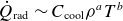 $\dot {Q}_{\text{rad}}\sim C_{\text{cool}}\rho ^aT^b$
in the MHD equation of state. The resultant equations (2.31) for
$\dot {Q}_{\text{rad}}\sim C_{\text{cool}}\rho ^aT^b$
in the MHD equation of state. The resultant equations (2.31) for
 $\xi (t)=x(t)/x_0$
and
$\xi (t)=x(t)/x_0$
and
 $\eta (t)=y(t)/y_0$
for the location of a plasma parcel originally at position (
$\eta (t)=y(t)/y_0$
for the location of a plasma parcel originally at position (
 $x_0$
,
$x_0$
,
 $y_0$
) are derived using Lagrangian MHD (see §§ 2.1–2.3) and account for the strength of radiative cooling using the cooling parameter
$y_0$
) are derived using Lagrangian MHD (see §§ 2.1–2.3) and account for the strength of radiative cooling using the cooling parameter
 $R=\tau _{\text{outflow}}/\tau _{\text{cool}}$
.
$R=\tau _{\text{outflow}}/\tau _{\text{cool}}$
.
The solutions to these equations are obtained numerically for bremsstrahlung cooling with values of
 $R$
ranging from
$R$
ranging from
 $R=3$
(weak cooling) to
$R=3$
(weak cooling) to
 $R=3000$
(strong cooling), and are compared with the solution with uniform pressure and no radiative cooling, as obtained by Syrovatskii (Reference Syrovatskii1971), and the solution with a non-uniform pressure and no radiative cooling (see § 3.1). The results, which can be seen by plotting the evolution of
$R=3000$
(strong cooling), and are compared with the solution with uniform pressure and no radiative cooling, as obtained by Syrovatskii (Reference Syrovatskii1971), and the solution with a non-uniform pressure and no radiative cooling (see § 3.1). The results, which can be seen by plotting the evolution of
 $\xi$
and
$\xi$
and
 $\eta$
(figure 1) and the contours of the magnetic flux function
$\eta$
(figure 1) and the contours of the magnetic flux function
 $\psi (x,y)$
(figure 2), show that stronger radiative cooling causes the X-point to collapse more rapidly in the inflow direction, and also results in a reversal of the direction of the outflows for sufficiently large values of
$\psi (x,y)$
(figure 2), show that stronger radiative cooling causes the X-point to collapse more rapidly in the inflow direction, and also results in a reversal of the direction of the outflows for sufficiently large values of
 $R$
.
$R$
.
The derived asymptotic behaviour of
 $\xi$
(see § 3.2) can be used to show that, for weak cooling, the radiative cooling term adds a corrective term that scales as
$\xi$
(see § 3.2) can be used to show that, for weak cooling, the radiative cooling term adds a corrective term that scales as
 $\sim (t_c-t)^{4/3}$
to the non-radiative asymptotic behaviour
$\sim (t_c-t)^{4/3}$
to the non-radiative asymptotic behaviour
 $\xi \sim (t_c-t)^{2/3}$
. For strong cooling, the cooling term dominates the asymptotic behaviour of
$\xi \sim (t_c-t)^{2/3}$
. For strong cooling, the cooling term dominates the asymptotic behaviour of
 $\xi$
(figure 3
b) resulting in a modified scaling of
$\xi$
(figure 3
b) resulting in a modified scaling of
 $\xi \sim (t_c-t)$
, which has a sharper scaling than that for weak cooling.
$\xi \sim (t_c-t)$
, which has a sharper scaling than that for weak cooling.
The reversal of flows along the
 $y$
-axis can be attributed to the non-uniform compression of the layer by the magnetic pressure, resulting in an inward thermal pressure gradient that opposes the
$y$
-axis can be attributed to the non-uniform compression of the layer by the magnetic pressure, resulting in an inward thermal pressure gradient that opposes the
 $\boldsymbol{j} \times \boldsymbol{B}$
force that drives the kinetic pressure gradient formed by the outflows. Naturally, a stronger
$\boldsymbol{j} \times \boldsymbol{B}$
force that drives the kinetic pressure gradient formed by the outflows. Naturally, a stronger
 $\boldsymbol{j} \times \boldsymbol{B}$
(stronger upstream magnetic field) yielding faster outflows reduces the impact of the inward thermal pressure gradient, and thus radiative cooling. The threshold for when this inward thermal pressure gradient is strong enough to decelerate the outflows is found to occur above a critical value of
$\boldsymbol{j} \times \boldsymbol{B}$
(stronger upstream magnetic field) yielding faster outflows reduces the impact of the inward thermal pressure gradient, and thus radiative cooling. The threshold for when this inward thermal pressure gradient is strong enough to decelerate the outflows is found to occur above a critical value of
 $R\equiv R^{\star } \approx 10$
. At
$R\equiv R^{\star } \approx 10$
. At
 $R^{\star }$
, the cooling term in the equation for
$R^{\star }$
, the cooling term in the equation for
 $\ddot {\xi }$
balances the
$\ddot {\xi }$
balances the
 $1/\xi ^2$
term near the finite-time singularity (see § 3.3).
$1/\xi ^2$
term near the finite-time singularity (see § 3.3).
Given the sharp magnetic field gradient across the width of the current sheet for
 $t\approx t_c$
, ohmic heating is expected to no longer be negligible around this time. Thus, we derived a steady-state solution for the radiatively cooled current sheet by modifying the compressible Sweet–Parker model derived by Uzdensky & McKinney (Reference Uzdensky and McKinney2011). Importantly, our modification includes the current sheet length as a variable, as our current sheet formation model predicts that, for strong cooling, the expected current sheet length will be shorter than the characteristic system size. This additional variable is solved for by imposing the condition
$t\approx t_c$
, ohmic heating is expected to no longer be negligible around this time. Thus, we derived a steady-state solution for the radiatively cooled current sheet by modifying the compressible Sweet–Parker model derived by Uzdensky & McKinney (Reference Uzdensky and McKinney2011). Importantly, our modification includes the current sheet length as a variable, as our current sheet formation model predicts that, for strong cooling, the expected current sheet length will be shorter than the characteristic system size. This additional variable is solved for by imposing the condition
 $\tau _A=\tau _{\text{cool}}$
, allowing for a given plasma parcel to travel the length of the layer before undergoing radiatively driven collapse (see § 4); this condition is required for the existence of a steady state. It is found that the radiative cooling results in an increased reconnection rate as compared with the Sweet–Parker reconnection rate for an incompressible plasma (4.15). Effectively, radiative cooling yields a contracted steady-state current sheet length compared with the system size (4.14), which in turn decreases the Lundquist number and thus results in a higher reconnection rate.
$\tau _A=\tau _{\text{cool}}$
, allowing for a given plasma parcel to travel the length of the layer before undergoing radiatively driven collapse (see § 4); this condition is required for the existence of a steady state. It is found that the radiative cooling results in an increased reconnection rate as compared with the Sweet–Parker reconnection rate for an incompressible plasma (4.15). Effectively, radiative cooling yields a contracted steady-state current sheet length compared with the system size (4.14), which in turn decreases the Lundquist number and thus results in a higher reconnection rate.
It is worth noting that, whilst this paper focuses on radiative cooling, radiation can have a myriad of important effects on magnetic reconnection in extreme astrophysical environments such as radiation pressure, Compton drag and, for extremely high energy densities, pair creation (Uzdensky Reference Uzdensky2011). In addition to this, reconnection layers in higher energy density environments can be optically thick to their dominant cooling mechanism, requiring the inclusion of the radiative transfer equations in the reconnection problem. Given the vast variety of processes that can be accounted for when modelling the interaction between radiation and reconnection, we have chosen to start by considering the simplest set up, involving the dominant effect of radiation, radiative cooling, that is optically thin in the relatively low energy density plasmas for which the Newtonian MHD framework is valid. Thus, influenced by the early progress made in modelling reconnection in the classical setting, the work in this paper provides a starting point for the development of a theoretical framework for reconnection processes in radiatively cooled plasmas. The findings in this paper lay the groundwork for future study on the impact of radiative cooling on reconnection beyond the Sweet–Parker model, including its interaction with the plasmoid instability, its impact on the global reconnection rate and extensions to non-MHD systems. With regards to the latter, it is encouraging that existing PIC simulations of reconnection with strong cooling reveal current sheets that are thinner than their counterparts formed in the absence of radiative cooling, in qualitative agreement with our findings (Nalewajko et al. Reference Nalewajko, Yuan and Chruślińska2018; Werner et al. Reference Werner, Philippov and Uzdensky2018; Sridhar et al. Reference Sridhar, Sironi and Beloborodov2021, Reference Sridhar, Sironi and Beloborodov2023). Interesting directions for future research include numerical verification of the results in this paper and a study on the inclusion of other important thermodynamic effects such as thermal conduction.
Acknowledgments
The authors would like to thank J. Hare and D. Uzdensky for valuable discussions on radiative cooling in reconnection layers. S.C acknowledges support from the MIT MathWorks and the NSE Manson Benedict fellowship awards.
Editor Alex Schekochihin thanks the referees for their advice in evaluating this article.
Declaration of interests
The authors have no conflicts of interest to disclose.
Appendix A
Here, we detail the method used to obtain the final form of the Lagrangian pressure
 $P_L$
in (2.24).
$P_L$
in (2.24).
Starting from the Lagrangian equation of state described by (2.23)
 \begin{equation} \frac {\partial }{\partial t} \ln \left [\frac {P_L}{\rho _L^\gamma }\right ]=-\overline {C}_{\text{cool}} \rho _L^{a-b} P_L^{b-1}, \end{equation}
we define an ansatz
 $P_L\rho _L^{-\gamma }=F(t,x,y)P_0\rho _0^{-\gamma }$
with
$P_L\rho _L^{-\gamma }=F(t,x,y)P_0\rho _0^{-\gamma }$
with
 $F(t,x,y=0)=1$
. To substitute this into the equation of state, we first rearrange the right-hand side term of the equation of state as follows:
$F(t,x,y=0)=1$
. To substitute this into the equation of state, we first rearrange the right-hand side term of the equation of state as follows:
 \begin{equation} \frac {P_L^{b-1}}{\rho _L^{b-a}}=\frac {P_L^{b-1}}{\rho _L^{\gamma (b-1)} \rho _L^{b-a} \rho _L^{-\gamma (b-1)}}. \end{equation}
Using the expression for Lagrangian density
 $\rho _L=\rho _0 / J$
, the following expression for
$\rho _L=\rho _0 / J$
, the following expression for
 $\rho _L^{a-b} P_L^{b-1}$
in terms of
$\rho _L^{a-b} P_L^{b-1}$
in terms of
 $F(x_0,y_0)$
,
$F(x_0,y_0)$
,
 $P_0$
,
$P_0$
,
 $\rho _0$
and
$\rho _0$
and
 $J(t,\boldsymbol{r}_0)$
is obtained:
$J(t,\boldsymbol{r}_0)$
is obtained:
 \begin{equation} \frac {P_L^{b-1}}{\rho _L^{b-a}}=F(x_0,y_0)^{b-1} \frac {P_0^{b-1}}{\rho _0^{b-a}} J(t,\boldsymbol{r}_0)^{b(1-\gamma )+(\gamma -a)}. \end{equation}
This expression thus encodes the time dependence of the left-hand side of the equation into
 $F(x_0,y_0)$
, which we have to solve for, and
$F(x_0,y_0)$
, which we have to solve for, and
 $J(t,\boldsymbol{r}_0)$
, which is evaluated to be
$J(t,\boldsymbol{r}_0)$
, which is evaluated to be
 $J(t,\boldsymbol{r}_0)=\xi \eta$
in (2.31). By simply substituting the expression in (A3) in the equation of state, the following partial differential equation in
$J(t,\boldsymbol{r}_0)=\xi \eta$
in (2.31). By simply substituting the expression in (A3) in the equation of state, the following partial differential equation in
 $F$
can be found:
$F$
can be found:
 \begin{equation} \frac {\partial }{\partial t} \ln \left [F \frac {P_0}{\rho _0^\gamma }\right ]=\frac {1}{F^{b-1}} \frac {\partial }{\partial t} \ln F=\frac {1}{F^b}\frac {\partial F}{\partial t}=-C_{t}\boldsymbol{\cdot} F^{b-1} P_0^{b-1} \rho _0^{a-b} J^{b(1-\gamma )+(\gamma -a)}. \end{equation}
Combining the homogeneous solution
 $C_1$
, which is a constant to be determined, with the particular solution that integrates over
$C_1$
, which is a constant to be determined, with the particular solution that integrates over
 $J(t,\boldsymbol{r}_0)$
results in the following general solution for
$J(t,\boldsymbol{r}_0)$
results in the following general solution for
 $F$
:
$F$
:
 \begin{equation} F=C_1-\frac {C_2(x_0, y_0)}{P_0}[(\gamma -1)(1-b)\overline {C}_{\text{cool}}\int _0^t J(t',\boldsymbol{r}_0)^{b(1-\gamma )+(\gamma -a)}\text{d}t^{\prime }]^{1/(1-b)}. \end{equation}
To completely specify
 $F$
, the constants
$F$
, the constants
 $C_1$
and
$C_1$
and
 $C_2$
need to be determined.
$C_2$
need to be determined.
 $C_1$
can be evaluated using the initial condition
$C_1$
can be evaluated using the initial condition
 $F(t=0,x_0,y_0)=1$
to simply be
$F(t=0,x_0,y_0)=1$
to simply be
 $C_1=1$
. On the other hand,
$C_1=1$
. On the other hand,
 $C_2(x_0,y_0)$
needs to be selected; we define it to be
$C_2(x_0,y_0)$
needs to be selected; we define it to be
 $P_{0}=P_{0,X}\left (1-(x_0^2+y_0^2)/2\right )$
. This expression is just a parabolic, non-uniform pressure profile used to model the plasma in this paper. It is noted that
$P_{0}=P_{0,X}\left (1-(x_0^2+y_0^2)/2\right )$
. This expression is just a parabolic, non-uniform pressure profile used to model the plasma in this paper. It is noted that
 $C_2(x_0,y_0)$
can take any spatial dependence given that the initial condition for
$C_2(x_0,y_0)$
can take any spatial dependence given that the initial condition for
 $F$
is satisfied regardless of the form of
$F$
is satisfied regardless of the form of
 $C_2(x_0,y_0)$
.
$C_2(x_0,y_0)$
.
Finally, substituting this expression for
 $F$
into the ansatz
$F$
into the ansatz
 $P_L\rho _L^{-\gamma }=F(t,x_0,y_0)P_0\rho _0^{-\gamma }$
, with the expression for
$P_L\rho _L^{-\gamma }=F(t,x_0,y_0)P_0\rho _0^{-\gamma }$
, with the expression for
 $\widetilde {C}_{\text{cool}}=\left [(\gamma -1)(b-1) R\right ]^{1/(1-b)}$
yields the expression required for
$\widetilde {C}_{\text{cool}}=\left [(\gamma -1)(b-1) R\right ]^{1/(1-b)}$
yields the expression required for
 $P_L$
$P_L$
 \begin{equation} P_L=\frac {P_0\left (x_0, y_0\right )}{J^\gamma } \times \left (1-\left [(\gamma -1)(1-b) R\int _0^t J^{b(1-\gamma )+(\gamma -a)}(t',\boldsymbol{r}_0) \text{d} t^{\prime }\right ]^{1 /(1-b)}\right )\!, \end{equation}
where
 $R\equiv \tau _{\text{outflow}}/\tau _{\text{cool}}$
is the cooling parameter.
$R\equiv \tau _{\text{outflow}}/\tau _{\text{cool}}$
is the cooling parameter.
Appendix B
Here, we justify and detail the method used to obtain the correction
 $\sim (t_c-t)^{4/3}$
to scaling for
$\sim (t_c-t)^{4/3}$
to scaling for
 $\xi$
for small values of
$\xi$
for small values of
 $R$
. First, we justify the use of our method by considering the alternative method employed in S71, starting with the equation obtained for
$R$
. First, we justify the use of our method by considering the alternative method employed in S71, starting with the equation obtained for
 $\ddot {\xi }$
(3.2), which is expressed in the limit of small
$\ddot {\xi }$
(3.2), which is expressed in the limit of small
 $R$
, near
$R$
, near
 $t\approx t_c$
 \begin{equation} \ddot {\xi } \approx -\eta \left (t_c\right )\left [\frac {1}{\xi ^2}+C_{\text{int}}(t_c-t)^{({2}/{3}) \alpha _p+({1}/{(1-b))}}\right ]; \quad \text{with } \alpha _p=\frac {b-a}{(1-b)}, \end{equation}
where
 $C_{\text{int}}$
is
$C_{\text{int}}$
is
 \begin{equation} C_{\text{int}}=\widetilde {C}_{\text{cool}} \left [\frac {9}{2} \eta (t_c)^4\right ]^{(b-a)/ 3(1-b)}\left [\frac {3}{2[b(1-\gamma )+(\gamma -a)]+3}\right ]^{1/(1-b)}. \end{equation}
Here, we are considering weak enough cooling such that there is no turning point in
 $\eta (t)$
and that
$\eta (t)$
and that
 $1/\xi ^2\gg 1/\eta ^2$
. As such, we take
$1/\xi ^2\gg 1/\eta ^2$
. As such, we take
 $\eta \approx \eta (t_c)$
and neglect the
$\eta \approx \eta (t_c)$
and neglect the
 $1/\eta ^2$
and
$1/\eta ^2$
and
 $1/(\xi \eta )^{\gamma }$
terms (
$1/(\xi \eta )^{\gamma }$
terms (
 $1/\xi ^2\gg 1/(\xi \eta )^{\gamma }$
as
$1/\xi ^2\gg 1/(\xi \eta )^{\gamma }$
as
 $\gamma =5/3 \lt 2$
).
$\gamma =5/3 \lt 2$
).
For bremsstrahlung radiation (
 $a=2,b=1/2)$
, this yields the following second-order ordinary differential equation (ODE) for
$a=2,b=1/2)$
, this yields the following second-order ordinary differential equation (ODE) for
 $\xi$
:
$\xi$
:
 \begin{equation} \ddot {\xi } \approx -\eta (t_c)\left (\frac {1}{\xi ^2}+C_{\text{int}}\right ) .\end{equation}
In S71, this second-order ODE is reduced to a first-order ODE by substituting the expression for
 $\ddot {\xi }$
in the following Taylor expansion, taken in the limit
$\ddot {\xi }$
in the following Taylor expansion, taken in the limit
 $t\approx t_c$
:
$t\approx t_c$
:
 \begin{equation} \xi (t_c)=0 \approx \xi (t)+(t_c-t)\dot {\xi }+\frac {(t_c-t)^2}{2}\ddot {\xi }+\mathcal{O}\left ((t_c-t)^3\right ). \end{equation}
Defining
 $(t_c-t)\equiv s$
, this yields the following first-order ODE for
$(t_c-t)\equiv s$
, this yields the following first-order ODE for
 $\xi$
in
$\xi$
in
 $s$
:
$s$
:
 \begin{equation} \xi ^3-\xi ^2s\frac {\text{d}\xi }{\text{d}s}-\eta (t_c)C_{\text{int}}\xi ^2s=\eta (t_c)s. \end{equation}
This equation can be identified as a form Chini’s equation; properties of this can be used to show that an analytic solution to this equation does not exist. Analytic solutions are possible for such equations if their corresponding Chini invariant (
 $I_{ch}$
, defined below) is independent of the variable (Kamke Reference Kamke1944). For the general form of Chini’s equation for some function
$I_{ch}$
, defined below) is independent of the variable (Kamke Reference Kamke1944). For the general form of Chini’s equation for some function
 $y(x)$
 \begin{equation} \frac {\text{d}y(x)}{\text{d}x}=f(x)y(x)^n-g(x)y(x)+h(x), \end{equation}
the expression for the Chini invariant
 $I_{ch}$
is defined as follows:
$I_{ch}$
is defined as follows:
 \begin{equation} I_{ch}=f(x)^{-(n+1)}h(x)^{-2n+1}\left (f(x)\frac {\text{d}h(x)}{\text{d}x}-h(x)\frac {\text{d}f(x)}{\text{d}x}-n\boldsymbol{\cdot} g(x)f(x)h(x)\right )^n \times n^{-n}. \end{equation}
Our differential equation can be re-expressed to match the general form of Chini’s equation
 \begin{equation} \frac {\text{d}\xi }{\text{d}s}=\frac {\xi }{s}-C_{\text{int}}\eta (t_c)-\frac {\eta (t_c)}{\xi ^{2}}, \end{equation}
yielding a corresponding Chini invariant
 \begin{equation} I_{ch}=[C_{\text{int}}\eta (t_c)^2]^{-3}\times \left (-2 \times C_{\text{int}}\eta (t_c)^2 \times \frac {1}{s}\right )^{-2}\times (-2)^{2}=[C_{\text{int}}\eta (t_c)^2]^{-5}s^2. \end{equation}
Here,
 $I_{ch}$
is clearly a function of the variable
$I_{ch}$
is clearly a function of the variable
 $s$
and thus there is no analytic solution for (B5). Thus, we choose to proceed using a different method, that employs the use of the Taylor expansion in (B4) at a later step.
$s$
and thus there is no analytic solution for (B5). Thus, we choose to proceed using a different method, that employs the use of the Taylor expansion in (B4) at a later step.
Returning to (B3) for bremsstrahlung radiation, we can use the substitution
 $\xi \equiv c_1^{1 / 3} z$
to yield the simpler equation
$\xi \equiv c_1^{1 / 3} z$
to yield the simpler equation
 \begin{equation} \ddot {z}=\frac {1}{z^2}+\frac {c_2}{c_1^{1 / 3}}, \end{equation}
where
 $c_1=-\eta (t_c)$
and
$c_1=-\eta (t_c)$
and
 $c_2=-C_{\text{int}} \eta (t_c)$
. Then, by simply integrating by parts, we can reduce this equation to the following first-order ODE:
$c_2=-C_{\text{int}} \eta (t_c)$
. Then, by simply integrating by parts, we can reduce this equation to the following first-order ODE:
 \begin{equation} \frac {1}{2}\left (\dot {z}\right )^2=c_3+\frac {c_2}{c_1^{1/3}} z-\frac {1}{z}, \end{equation}
where
 $c_3=c_1^{1 / 3}(c_1^{-1 / 3}/2-c_2c_1^{2 / 3})$
. By rearranging this ODE and integrating over time, a solution in the functional form
$c_3=c_1^{1 / 3}(c_1^{-1 / 3}/2-c_2c_1^{2 / 3})$
. By rearranging this ODE and integrating over time, a solution in the functional form
 $\Delta t(z)$
, where
$\Delta t(z)$
, where
 $\Delta t=(t_c-t)$
, can be obtained
$\Delta t=(t_c-t)$
, can be obtained
 \begin{equation} \left (t_c-t\right )+c_4=\int ^{\xi (t_c)}_{\xi _0} \sqrt {\frac {\xi }{c_3 c_1^{2 / 3} \xi +c_2 \xi ^2-c_1} }\,\text{d} \xi , \end{equation}
where
 $c_4=0$
as
$c_4=0$
as
 $\xi (t=t_c)=0$
. Treating
$\xi (t=t_c)=0$
. Treating
 $\xi$
as the relevant small parameter, the integrand can be expanded to yield
$\xi$
as the relevant small parameter, the integrand can be expanded to yield
 \begin{align} \left (t_c-t\right ) &\approx \int \sqrt {-\frac {1}{c_1} \xi }-\frac {1}{2} \xi ^{3/2}\left (c_3 c_1^{2/3} \sqrt {-\frac {1}{c_1}}\right )+\mathcal{O}\left (\xi ^{5/2}\right ) \,\text{d} \xi \nonumber\\[5pt] & \approx \frac {2}{3} \sqrt {-\frac {1}{c_1}} \xi ^{3/2}-\frac {1\left (c_3 c_1^{2/3} \sqrt {-\frac {1}{c_1}}\right )}{5} \xi ^{5/2}+\mathcal{O}\left (\xi ^{7/2}\right ). \end{align}
Lastly, substituting the ansatz
 $\xi \sim (9\eta (t_c)/4)^{1/3}(t_c-t)^{2/3}+c_\alpha (t_c-t)^{\alpha }$
, and keeping terms up to
$\xi \sim (9\eta (t_c)/4)^{1/3}(t_c-t)^{2/3}+c_\alpha (t_c-t)^{\alpha }$
, and keeping terms up to
 $\mathcal{O}(\xi ^{5/2})$
gives
$\mathcal{O}(\xi ^{5/2})$
gives
 $\alpha =4/3$
, yielding the required scaling for
$\alpha =4/3$
, yielding the required scaling for
 $\xi$
$\xi$
 \begin{equation} \xi \sim \left (\frac {9}{4}\eta (t_c)\right )^{1/3}(t_c-t)^{2/3}+\frac {2}{15}\left (\frac {9}{4}\right )^{13/6}c_3(-c_1)^{7/3}(t_c-t)^{4/3}. \end{equation}


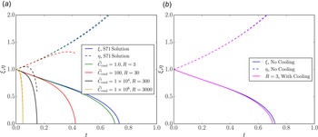


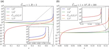


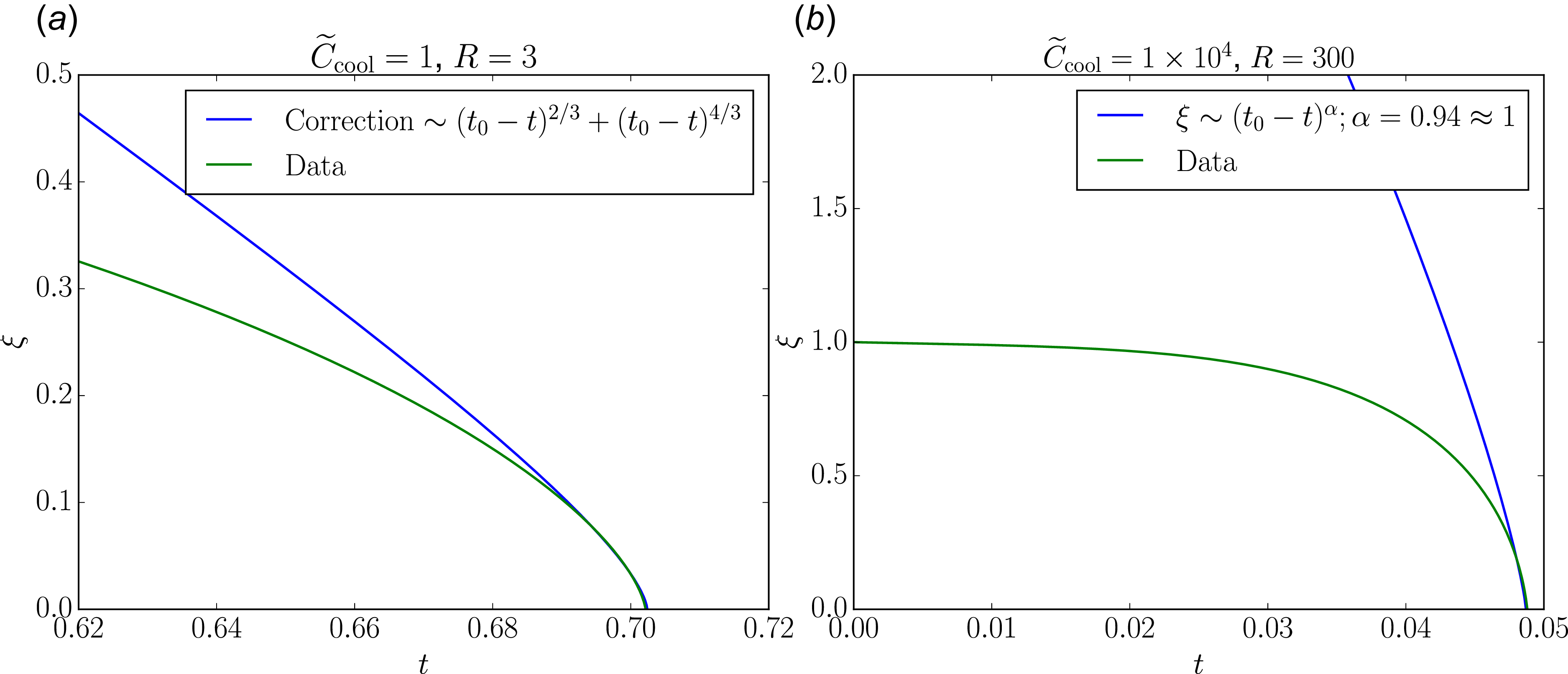


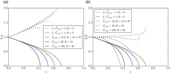


 Open access