


1. Introduction
Shock-containing shear flows involve a rich variety of phenomena including shock–turbulence interaction (STI). In free shear layers, STI leads to an increase in turbulence levels and mixing downstream of the shock (Génin & Menon Reference Génin and Menon2010). In wall-bounded flows, in addition to the enhancement of turbulence, STI may also be accompanied by boundary layer separation and the formation of a separation bubble (Delery Reference Delery1983; Dolling Reference Dolling2001; Clemens & Narayanaswamy Reference Clemens and Narayanaswamy2014). The STI is also an important feature of supersonic combustion in scramjets (Yang, Kubota & Zukoski Reference Yang, Kubota and Zukoski1993). In imperfectly expanded propulsive jets, STI underpins the generation of broad-band shock associated noise (Tanna Reference Tanna1977; Tam & Tanna Reference Tam and Tanna1982) and screech (Powell Reference Powell1953; Tam, Seiner & Yu Reference Tam, Seiner and Yu1986; Raman Reference Raman1999; Edgington-Mitchell Reference Edgington-Mitchell2019).
Linear theory has been widely used to study the interaction between disturbance fields and shocks. Ribner (Reference Ribner1954) considered the interaction between a vorticity wave and a normal shock. The analysis was later extended to consider STI, where a homogeneous turbulence was modelled as a superposition of Fourier vorticity waves (Ribner Reference Ribner1955). Moore (Reference Moore1954) considered the interaction between sound waves and an oblique shock, and this work was extended by Mahesh et al. (Reference Mahesh, Lee, Lele and Moin1995) to study an isotropic field of acoustic disturbances interacting with a shock. Later, Mahesh, Lele & Moin (Reference Mahesh, Lele and Moin1997) considered the influence of entropy fluctuations on STI as well and Buttsworth (Reference Buttsworth1996) derived expressions for shock-induced vorticity, useful for the estimation of mixing enhancement. The foregoing studies were all based on solution of the Rankine–Hugoniot relations. The unsteady STI was converted into an equivalent steady-flow problem which did not consider the reflection process associated with the incident turbulent disturbance but only the transmission mechanism through the shock wave. A review of these studies and others has been compiled by Andreopoulos, Agui & Briassulis (Reference Andreopoulos, Agui and Briassulis2000). More recently, Kitamura et al. (Reference Kitamura, Nagata, Sakai, Sasoh and Ito2016) used rapid distortion theory to study the interaction between homogeneous isotropic turbulence and a shock wave, and Chen & Donzis (Reference Chen and Donzis2019) considered STI at high turbulence intensities. Similarly to the works reported above, the authors mainly focused on the turbulence amplification and modification of the turbulence length scales downstream of the shock.
The reflection and transmission of acoustic, vorticity and entropy waves within a convergent–divergent nozzle with and without a shock was studied by Marble & Candel (Reference Marble and Candel1977). The study focused on compact disturbances, that is, with wavelengths larger than the nozzle length, thus limiting the application to low frequencies. The inclusion of non-compactness effects was considered by Stow, Dowling & Hynes (Reference Stow, Dowling and Hynes2002), who provided a first-order correction for the phase of the reflection coefficient for higher frequencies. The correction was extended to the transmission coefficient also by Goh & Morgans (Reference Goh and Morgans2011) and a further development was carried out by Duran & Moreau (Reference Duran and Moreau2013) and Duran & Morgans (Reference Duran and Morgans2015), who extended the high-frequency correction to the amplitude of the reflection and transmission coefficients in the case of planar and circumferential incident waves, respectively. All of these works were motivated by the problem of combustion noise and the role the reflected waves play on the onset of thermo-acoustic instability in the combustion chamber of the burner–turbine–nozzle configuration of an aero-engine.
The problem we consider is motivated by the sound generated by imperfectly expanded, supersonic jets and, in particular, the phenomenon known as screech, a mechanistic explanation for which was first provided by Powell (Reference Powell1953). The mechanism involves turbulent structures that are convected through the shock-cell structure; this STI results in the generation of upstream-travelling sound waves. According to Powell's phenomenological description, when the phases of the upstream-travelling sound waves and downstream-travelling turbulent structures are suitably matched, at the jet exit plane and at the STI locations, resonance may occur. The downstream-travelling turbulent structures considered important for screech are what are often referred to as coherent structures.
A large body of recent work has shown how coherent structures in turbulent jets, and the sound they produce, can be modelled using linear theory (Jordan & Colonius Reference Jordan and Colonius2013; Schmidt et al. Reference Schmidt, Towne, Colonius, Cavalieri, Jordan and Brès2017; Towne, Schmidt & Colonius Reference Towne, Schmidt and Colonius2018; Cavalieri, Jordan & Lesshafft Reference Cavalieri, Jordan and Lesshafft2019; Lesshafft et al. Reference Lesshafft, Semeraro, Jaunet, Cavalieri and Jordan2019; Nogueira et al. Reference Nogueira, Cavalieri, Jordan and Jaunet2019; Edgington-Mitchell et al. Reference Edgington-Mitchell, Wang, Nogueira, Schmidt, Jaunet, Duke, Jordan and Towne2021a). As shown in these studies, downstream-travelling coherent structures are largely underpinned by Kelvin–Helmholtz (K–H) instability. Powell (Reference Powell1953) assumed that the upstream-travelling waves responsible for the feedback mechanism in screech generation were free-stream acoustic waves, but this has been recently questioned. Shen & Tam (Reference Shen and Tam2002) suggested that the upstream-travelling disturbance might comprise a family of guided jet modes, first discussed by Tam & Hu (Reference Tam and Hu1989). This hypothesis has been recently confirmed in studies by Gojon, Bogey & Mihaescu (Reference Gojon, Bogey and Mihaescu2018) and Edgington-Mitchell et al. (Reference Edgington-Mitchell, Jaunet, Jordan, Towne, Soria and Honnery2018), and a simplified screech-tone prediction model based on this idea has been developed and validated by Mancinelli et al. (Reference Mancinelli, Jaunet, Jordan and Towne2019a). In the simplest formulation of the screech-tone model, the spatial growth of the K–H mode is ignored, and a phase-matching criterion is sufficient to provide a reasonable prediction of screech-tone frequencies. A similar resonant mechanism was proposed for subsonic compressible jets (Towne et al. Reference Towne, Cavalieri, Jordan, Colonius, Schmidt, Jaunet and Brès2017), cavity flows (Rossiter Reference Rossiter1964; Rowley, Colonius & Basu Reference Rowley, Colonius and Basu2002) and impinging jets (Tam & Ahuja Reference Tam and Ahuja1990; Bogey & Gojon Reference Bogey and Gojon2017). The reflection of waves is implicitly considered in all these mechanisms, but it is rarely studied in detail. In more complete screech-frequency prediction models (Mancinelli et al. Reference Mancinelli, Jaunet, Jordan, Towne and Girard2019b, Reference Mancinelli, Jaunet, Jordan and Towne2021), where the spatial growth rates of the upstream- and downstream-travelling waves are included, knowledge of the reflection coefficients in the jet exit plane and at the location of STI is required.
In this paper, we investigate the interaction between a downstream-travelling K–H wave and a normal shock and compute the amplitude and phase of the reflected upstream-travelling guided wave active in the screech loop using a mode-matching approach. We consider vortex-sheet (V-S) and finite-thickness (F-T) flow models, which elucidate the role of shear in the reflection and transmission processes. The efficiency of the mode-matching technique in the presence of a discontinuity, as is the shock in the flow we consider herein, has been already shown by Gabard & Astley (Reference Gabard and Astley2008) for the estimation of the sound attenuation in a lined duct. More recently, a mode-matching approach has been used by Dai (Reference Dai2020, Reference Dai2021) to calculate the reflection and transmission coefficients in a duct flow in the presence of a cavity. Consistent with these works, we use linear theory to describe the flow dynamics upstream and downstream of the shock and then match the solutions across the discontinuity.
The paper is organised as follows. The general modelling framework, including the jet models adopted and the mode-matching approach used to calculate the reflection and transmission coefficients, is presented in § 2. Results involving the reflection-coefficient calculation, its dependence on the frequency and jet-flow conditions and the reflected and transmitted pressure fields are presented and discussed in § 3. The paper closes with concluding remarks in § 4.
2. Modelling framework
We here present the shock and jet-dynamics modelling and the procedure adopted to calculate the reflection and transmission coefficients. We consider an axisymmetric, shock-containing supersonic jet. It is known that the organised structure of the jet plume of imperfectly expanded supersonic jets is shaped by oblique shocks and expansion waves (see the many flow visualisations presented in Powell Reference Powell1953; Powell, Umeda & Ishii Reference Powell, Umeda and Ishii1992; Panda Reference Panda1999; Mercier, Castelain & Bailly Reference Mercier, Castelain and Bailly2017). Normal shocks are, however, found in the form of Mach disks for highly imperfectly expanded jets and often encountered in the jet plume of convergent–divergent nozzles and impinging jets (Edgington-Mitchell Reference Edgington-Mitchell2019). Despite many years of research activity (see the many works by Powell Reference Powell1953; Tam & Tanna Reference Tam and Tanna1982; Suzuki & Lele Reference Suzuki and Lele2003; Lele Reference Lele2005; Edgington-Mitchell et al. Reference Edgington-Mitchell, Weightman, Lock, Kirby, Nair, Soria and Honnery2021b), a clear picture of the way by which instability waves interact with shock cells to generate screech is still far from being reached. With the aim of keeping the model as simple as possible and in the absence of a clear and unambiguous description of the interaction between instability and shock waves, the shock is herein assumed to be normal, thus allowing the use of the locally parallel-flow assumption both upstream and downstream of the shock. This assumption implies that the linear response to shock oscillations induced by the incoming instability wave, which is a typical non-parallel feature, is not considered. A sketch of the shock-containing jet and the cylindrical reference system used in this paper are depicted in figure 1. We consider a K–H wave with unitary amplitude,  $I=1$, incident to a shock. The interaction of the incoming wave with the shock generates a collection of reflected and transmitted modes upstream and downstream of the shock, respectively. The sections upstream and downstream of the shock are hereinafter denoted 1 and 2 and the reflection and transmission coefficients of each wave moving away from the shock are indicated with $R_{n_R}$ and $T_{n_T}$, respectively. The state vector is $\boldsymbol {q}^*=\lbrace \rho ^*, u_x^*, u_r^*, u_\theta ^*, T^*, p^*\rbrace$, where $\rho$ is the flow density, u the velocity, T the temperature and p the pressure. The flow variables are normalised by the nozzle diameter $D$ and the ambient density and speed of sound $\rho _\infty$ and $c_\infty$, respectively, thus leading to a non-dimensional state vector $\boldsymbol {q}$.
Schematic representation of the jet model: (a) sketch of the shock-containing jet, (b) control volume representation with identification of the normal to the inlet and outlet surfaces.

2.1. Shock model
The flow regions upstream and downstream of the shock are well described by a locally parallel model. In order to connect these two regions, we impose the conservation laws of mass, momentum and energy through the shock. This is done by dividing the shock into infinitesimal control volumes  $\mathrm {d}V$ of length ${\rm \Delta} x\to 0$ such that the flux terms through the top and bottom surfaces are zero (see figure 1) and enforcing mass, momentum and energy conservation for the control volume, leading to the system of equations
 \begin{gather}\left.\begin{aligned} &\int_{S_1}\rho^*\boldsymbol{u}^*\boldsymbol{\cdot}\boldsymbol{n}\,\mathrm{d}S + \int_{S_2}\rho^*\boldsymbol{u}^*\boldsymbol{\cdot}\boldsymbol{n}\,\mathrm{d}S=0,\\ &\int_{S_1}\rho^*\boldsymbol{u}^*\left(\boldsymbol{u}^*\boldsymbol{\cdot}\boldsymbol{n}\right)\mathrm{d}S + \int_{S_1} p^*\boldsymbol{n}\,\mathrm{d}S + \int_{S_2}\rho^*\boldsymbol{u}^* \left(\boldsymbol{u}^*\boldsymbol{\cdot}\boldsymbol{n}\right)\mathrm{d}S - \int_{S_2} p^*\boldsymbol{n}\,\mathrm{d}S=0,\\ &\int_{S_1}\rho^* \,{\rm e}^*\boldsymbol{u}^*\boldsymbol{\cdot}\boldsymbol{n}\,\mathrm{d}S + \int_{S_2}\rho^* \,{\rm e}^*\boldsymbol{u}^*\boldsymbol{\cdot}\boldsymbol{n}\,\mathrm{d}S=0, \end{aligned}\right\} \end{gather}
where  ${\rm e}^*=h^*+0.5(u_x^{*2}+u_r^{*2}+u_\theta ^{*2})$ is the total specific energy with the enthalpy expressed as $h^*=c_pT^*$, $c_p$ is the specific heat capacity, S is the control volume surface and n the normal to the surface. Normalising the flow variables, performing the Reynolds decomposition,
 \begin{equation} \boldsymbol{q}\left(x,r,\theta,t\right)=\bar{\boldsymbol{q}}\left(r\right)+ \boldsymbol{q}'\left(x,r,\theta,t\right), \end{equation}
and substituting into (2.1a), removing the mean and linearising, the linearised jump equations for the shock become
 \begin{gather}\left.\begin{aligned} &\bar{u}_{1x}\rho_1+\bar{\rho}_1u_{1x}=\bar{u}_{2x} \rho_2+\bar{\rho}_2u_{2x},\\ &p_1+2\bar{\rho}_1\bar{u}_{1x}u_{1x}+\bar{u}_{1x}^2 \rho_1=p_2+2\bar{\rho}_2\bar{u}_{2x}u_{2x}+\bar{u}_{2x}^2\rho_2,\\ &u_{1r}=u_{2r},\\ &u_{1\theta}=u_{2\theta},\\ &T_1+\bar{u}_{1x}u_{1x}=T_2+\bar{u}_{2x}u_{2x}, \end{aligned}\right\} \end{gather}
where we removed the primes from the fluctuating variables for notational simplicity. We note that the adiabatic relation between the thermodynamic variables is implicit in the linearised operator. The perturbations upstream and downstream of the shock are modelled using the normal mode ansatz
 \begin{equation} \boldsymbol{q}'\left(x,r,\theta,t\right)=\hat{\boldsymbol{q}} \left(r\right)\exp({{\rm i}\left(kx+m\theta -\omega t\right)}), \end{equation}
where  $k$ is the wavenumber along the axial direction, $m$ is the azimuthal order and $\omega =2{\rm \pi} St M_a$ is a non-dimensional frequency, with $St=fD/U_j$ the nozzle-diameter-based Strouhal number, $M_a=U_j/c_\infty$ the acoustic Mach number, f the frequency, D the nozzle diameter and $U_j$ the fully expanded jet velocity. Considering that the only incident wave is the K–H wave, the system of (2.3a) can be written in a compact form as follows:
 \begin{equation}
\boldsymbol{\mathsf{A}}_1\left(I\hat{\boldsymbol{q}}_{1I}+
\sum_{n_R=1}^\infty
R_{n_R}\hat{\boldsymbol{q}}_{1R,n_R}\right)=
\boldsymbol{\mathsf{A}}_2\sum_{n_T=1}^\infty
T_{n_T}\hat{\boldsymbol{q}}_{2T,n_T},
\end{equation}
\begin{equation}
\boldsymbol{\mathsf{A}}_1\left(I\hat{\boldsymbol{q}}_{1I}+
\sum_{n_R=1}^\infty
R_{n_R}\hat{\boldsymbol{q}}_{1R,n_R}\right)=
\boldsymbol{\mathsf{A}}_2\sum_{n_T=1}^\infty
T_{n_T}\hat{\boldsymbol{q}}_{2T,n_T},
\end{equation}
where  $\hat {\boldsymbol {q}}_{1I}$, $\hat {\boldsymbol {q}}_{1R,n_R}$ and $\hat {\boldsymbol {q}}_{2T,n_T}$ are the incident, reflected and transmitted waves moving upstream and downstream of the shock, respectively, and
 \begin{equation} \boldsymbol{\mathsf{A}}_1=\begin{bmatrix} \bar{u}_{1x} & \bar{\rho}_1 & 0 & 0 & 0 & 0\\ \bar{u}_{1x}^2 & 2\bar{\rho}_1\bar{u}_{1x} & 0 & 0 & 0 & 1\\ 0 & 0 & 1 & 0 & 0 & 0\\ 0 & 0 & 0 & 1 & 0 & 0\\ 0 & \bar{u}_{1x} & 0 & 0 & 1 & 0 \end{bmatrix},\quad \boldsymbol{\mathsf{A}}_2= \begin{bmatrix} \bar{u}_{2x} & \bar{\rho}_2 & 0 & 0 & 0 & 0\\ \bar{u}_{2x}^2 & 2\bar{\rho}_2\bar{u}_{2x} & 0 & 0 & 0 & 1\\ 0 & 0 & 1 & 0 & 0 & 0\\ 0 & 0 & 0 & 1 & 0 & 0\\ 0 & \bar{u}_{2x} & 0 & 0 & 1 & 0 \end{bmatrix} \end{equation}
are matrices containing information about the mean flow upstream and downstream of the shock. The vector of eigenfunctions  $\hat {\boldsymbol {q}}_{1I}$, $\hat {\boldsymbol {q}}_{1R,n_R}$ and $\hat {\boldsymbol {q}}_{2T,n_T}$ are computed using either a V-S or F-T model (see § 2.3). The procedure used to ascertain whether a wave is reflected or transmitted is described in § 2.3.3.
2.2. Reflection- and transmission-coefficient calculation
Equation (2.5) is exact if a complete basis of jet modes is considered. In order to estimate the reflection- and transmission-coefficient values, we truncate the sum to a finite number of modes  $N_R$ and $N_T$ and we introduce an error density $\epsilon (r)$ for each conservation equation. Equation (2.5) can then be written as
 \begin{equation} \boldsymbol{\mathsf{A}}_1\left(I\hat{\boldsymbol{q}}_{1I}+\sum_{n_R=1}^{N_R} R_{n_R} \hat{\boldsymbol{q}}_{1R,n_R}\right)-\boldsymbol{\mathsf{A}}_2\sum_{n_T=1}^{N_T} T_{n_T} \hat{\boldsymbol{q}}_{2T,n_T}=\boldsymbol{\epsilon}, \end{equation}
where  $\boldsymbol {\epsilon }(r)$ is the error density vector and $\boldsymbol {\epsilon }\to 0$ if the number of modes $N_R$ and $N_T\to \infty$. The reflection and transmission coefficients $R_{n_R}$ and $T_{n_T}$ associated with each mode are estimated by a least-mean-square minimisation of the error densities, formalised as
 \begin{equation} \left[R_{opt,n_R},T_{opt,n_T}\right]=\underset{R_{n_R},T_{n_T} \in \mathcal{C}}{\text{min}}\underbrace{\int_0^\infty\vert\boldsymbol{\epsilon}^2\left(r\right)\vert\,\mathrm{d}r}_{F}. \end{equation}
 The objective function  $F$ corresponds to the sum of the absolute value of the squared error densities associated with each conservation equation integrated along the radial direction. To solve the minimisation problem in (2.8), we write (2.7) in a matrix form
 \begin{equation} \begin{bmatrix} \boldsymbol{\mathsf{A}}_1\hat{\boldsymbol{\mathsf{Q}}}_{1R}\quad -\boldsymbol{\mathsf{A}}_2\hat{\boldsymbol{\mathsf{Q}}}_{2T} \end{bmatrix} \begin{Bmatrix} \boldsymbol{R}\\ \boldsymbol{T} \end{Bmatrix} ={-}I\boldsymbol{\mathsf{A}}_1\hat{\boldsymbol{q}}_{1I}+\boldsymbol{\epsilon}, \end{equation}
where  $\hat {\boldsymbol{\mathsf{Q}}}_{1R}=[\hat {\boldsymbol {q}}_{1R,1},\ldots,\hat {\boldsymbol {q}}_{1R,N_R}]$ and $\hat {\boldsymbol{\mathsf{Q}}}_{2T}=[\hat {\boldsymbol {q}}_{2T,1},\ldots,\hat {\boldsymbol {q}}_{2T,N_T}]$ are the matrices of the eigenfunctions and $\boldsymbol {R}$ and $\boldsymbol {T}$ are the vectors of the reflection and transmission coefficients, respectively. We then define
 \begin{equation} \begin{Bmatrix} \boldsymbol{R}\\ \boldsymbol{T} \end{Bmatrix} = \boldsymbol{X},\quad \begin{bmatrix} \boldsymbol{\mathsf{A}}_1\hat{\boldsymbol{\mathsf{Q}}}_{1R} \quad -\boldsymbol{\mathsf{A}}_2\hat{\boldsymbol{\mathsf{Q}}}_{2T} \end{bmatrix} =\boldsymbol{\mathsf{B}},\quad \boldsymbol{y}=\boldsymbol{\mathsf{A}}_1\hat{\boldsymbol{q}}_{1I}I, \end{equation}
so that (2.9) can be written in the compact form  $\boldsymbol {\epsilon }=\boldsymbol {B}\boldsymbol {X}+\boldsymbol {y}$. The solution of (2.8) is obtained by finding the stationary point of $F$ by setting its gradient to zero
 \begin{equation} \frac{{\rm d} F}{{\rm d}\kern0.06em\boldsymbol{X}}=\frac{{\rm d}\left(\boldsymbol{\epsilon^T} \boldsymbol{W}\boldsymbol{\epsilon}\right)}{{\rm d}\kern0.06em\boldsymbol{X}} = \boldsymbol{B}^{\rm T}\boldsymbol{W}\boldsymbol{B}\boldsymbol{X}+ \boldsymbol{B}^{\rm T}\boldsymbol{\mathsf{W}}\boldsymbol{y}=0, \end{equation}
which leads to
 \begin{equation} \boldsymbol{X}={-}\left(\boldsymbol{B}^{\rm T}\boldsymbol{W}\boldsymbol{B}\right)^{{-}1} \boldsymbol{B}^{\rm T}\boldsymbol{W}\boldsymbol{y}, \end{equation}
where  $\boldsymbol {B}\vert _W^+=(\boldsymbol {B}^{\rm T}\boldsymbol {W}\boldsymbol {B})^{-1}\boldsymbol {B}^{\rm T}\boldsymbol {W}$ is the weighted pseudo-inverse matrix and $\boldsymbol {W}$ is a diagonal matrix of elements $dr$.
$dr$.
2.3. Jet models
We here present a local description of the jet dynamics using the parallel-flow linear stability theory. This theory is applied to two different models: a F-T flow model and a simplified cylindrical vortex sheet. Both are governed by the linearised Euler equations (LEE) (see Appendix A).
2.3.1. Finite-thickness model
Writing the LEE exclusively in terms of pressure, the compressible Rayleigh equation (Schmid & Henningson Reference Schmid and Henningson2001)
 \begin{align} & \frac{\partial^2\hat{p}}{\partial r^2}+\left(\frac{1}{r}-\frac{2k}{\bar{u}_xk-\omega} \frac{\partial\bar{u}_x}{\partial r}-\frac{\gamma -1}{\gamma\bar{\rho}} \frac{\partial\bar{\rho}}{\partial r}+\frac{1}{\gamma\bar{T}} \frac{\partial\bar{T}}{\partial r}\right) \frac{\partial\hat{p}}{\partial r} \nonumber\\ &\quad -\left(k^2+\frac{m^2}{r^2}- \frac{\left(\bar{u}_xk-\omega\right)^2}{\left(\gamma -1\right)\bar{T}}\right)\hat{p}=0, \end{align}
is obtained, where  $\gamma$ is the specific heat ratio for a perfect gas. The solution of the linear stability problem is obtained by specifying a real or complex frequency $\omega$ and solving the resulting augmented eigenvalue problem $k=k(\omega )$, with $\hat {p}(r)$ the associated pressure eigenfunction. The eigenvalue problem is solved numerically by discretising (2.13) in the radial direction using the Chebyshev polynomials and by imposing Dirichlet boundary conditions at the domain boundaries. A mapping function proposed by Lesshafft & Huerre (Reference Lesshafft and Huerre2007) is used to non-uniformly distribute the 500 grid points to efficiently resolve the shear layer of the jet and to ensure convergence of the computed eigenmodes. The eigenfunctions $\hat {u}_i$, $\hat {\rho }$ and $\hat {T}$ are calculated from the knowledge of $\hat {p}$ (see Appendix A). The eigenfunctions are normalised such that $\angle \hat {p}(r)=0$ for $r=0$ and to have unitary energy norm, which, following Chu (Reference Chu1965) and Hanifi, Schmid & Henningson (Reference Hanifi, Schmid and Henningson1996), is defined as
 \begin{equation} E=\frac{1}{2}\int_0^{2{\rm \pi}}\int_0^\infty \left(\bar{\rho}\left(\vert \widehat{u_x}\vert^2+\vert \widehat{u_r}\vert^2+\vert \widehat{u_\theta}\vert^2\right) + \frac{\gamma -1}{\gamma} \frac{\bar{T}}{\bar{\rho}}\vert\hat{\rho}\vert^2 + \frac{\bar{\rho}}{\gamma\bar{T}}\vert \hat{T}\vert^2\right)r\mathrm{d}r\,\mathrm{d}\theta. \end{equation}
The derivation of the energy norm is provided in Appendix B.
2.3.2. Vortex-sheet model
The V-S model is an inviscid idealisation of the jet where the infinitely thin V-S separates the interior flow and the outer quiescent fluid, resulting in a jet with a mean top-hat profile. The V-S was used by Lessen, Fox & Zien (Reference Lessen, Fox and Zien1965) and Michalke (Reference Michalke1970) to study the stability properties of a compressible jet. We recently showed that the standard V-S model for free jets, which was used in the previous studies, does not support free-stream acoustic waves as discrete modes, as required for the mode-matching procedure. To obtain a discrete representation of free-stream acoustic modes, we use the dispersion relation of a confined jet with the radial distance of the boundary ( $r_{MAX}$) sufficiently distant from the jet in order to recover the same dynamical properties of a free jet. The analysis of this surrogate problem allowed us to include the free-stream acoustic modes in the description of the jet dynamics (for more details the reader can refer to Mancinelli et al. Reference Mancinelli, Martini, Jaunet and Jordan2022). We herein use this confined version of the V-S, whose dispersion relation $D(k,\omega ;M_a,T,m,r_{MAX})=0$ is,
 \begin{equation} \begin{gathered}
\frac{1}{\left(1-\dfrac{kM_a}{\omega}\right)^2} +
\frac{1}{T}\frac{I_m\left(\dfrac{\gamma_i}{2}\right)}{K_m\left(\dfrac{\gamma_o}{2}\right)-zI_m
\left(\dfrac{\gamma_o}{2}\right)}\\
\frac{\dfrac{\gamma_o}{2}K_{m-1}\left(\dfrac{\gamma_o}{2}\right)
+
mK_m\left(\dfrac{\gamma_o}{2}\right)+z\left(\dfrac{\gamma_o}{2}I_{m-1}
\left(\dfrac{\gamma_o}{2}\right)-mI_m\left(\dfrac{\gamma_o}{2}\right)\right)}{\dfrac{\gamma_i}{2}I_{m-1}
\left(\dfrac{\gamma_i}{2}\right) -
mI_m\left(\dfrac{\gamma_i}{2}\right)}=0,
\end{gathered}
\end{equation}
\begin{equation} \begin{gathered}
\frac{1}{\left(1-\dfrac{kM_a}{\omega}\right)^2} +
\frac{1}{T}\frac{I_m\left(\dfrac{\gamma_i}{2}\right)}{K_m\left(\dfrac{\gamma_o}{2}\right)-zI_m
\left(\dfrac{\gamma_o}{2}\right)}\\
\frac{\dfrac{\gamma_o}{2}K_{m-1}\left(\dfrac{\gamma_o}{2}\right)
+
mK_m\left(\dfrac{\gamma_o}{2}\right)+z\left(\dfrac{\gamma_o}{2}I_{m-1}
\left(\dfrac{\gamma_o}{2}\right)-mI_m\left(\dfrac{\gamma_o}{2}\right)\right)}{\dfrac{\gamma_i}{2}I_{m-1}
\left(\dfrac{\gamma_i}{2}\right) -
mI_m\left(\dfrac{\gamma_i}{2}\right)}=0,
\end{gathered}
\end{equation}
with
 \begin{equation} \left.\begin{gathered} \gamma_i = \sqrt{k^2-\frac{1}{T}\left(\omega-M_ak\right)^2},\\ \gamma_o = \sqrt{k^2-\omega^2}, \end{gathered}\right\} \end{equation}
where  $I$ and $K$ are modified Bessel functions of the first and second kinds, respectively, $T=T_j/T_\infty$ is the jet-to-ambient temperature ratio such that the relation between the jet and the acoustic Mach numbers is $M_a=M_j\sqrt {T}$ and $z=K_m(\gamma _or_{MAX})/I_m(\gamma _or_{MAX})$. The branch cut in the square root of (2.16) is chosen such that $-{\rm \pi} /2\leq \rm {arg}(\gamma _{i,o})<{\rm \pi} /2$. The dispersion relation in (2.15) for a confined jet differs from the unconfined one for a free jet in the additional terms containing $z(r_{MAX})$. Following Mancinelli et al. (Reference Mancinelli, Martini, Jaunet and Jordan2022), we herein use $r_{MAX}=100$ in order to avoid any effect of the boundary on the eigenmodes. Frequency/wavenumber pairs $(\omega, k)$ that satisfy (2.15) define eigenmodes of the vortex sheet for given values of $m$,
$m$,  $M_a$, $T$ and $r_{MAX}$. To find these pairs, similarly to the F-T model, we specify a frequency $\omega$ (real or complex) and compute the associated eigenvalues $k$. Eigenvalues are computed using a root finder based on the Levenberg–Marquardt method (Levenberg Reference Levenberg1944; Marquardt Reference Marquardt1963).
After imposing bounded solution for  $r=0$ and a soft-wall boundary condition at $r=r_{MAX}$, the solution for the pressure in the inner and outer flows is
 \begin{gather}\left.\begin{aligned}
&\hat{p}_i\left(r\right)=B_iI_m\left(\gamma_ir\right)\quad
r\leq 0.5\\
&\hat{p}_o\left(r\right)=C_o\left({-}zI_m\left(\gamma_or\right)
+ K_m\left(\gamma_or\right)\right) \quad r> 0.5,
\end{aligned}\right\}
\end{gather}
\begin{gather}\left.\begin{aligned}
&\hat{p}_i\left(r\right)=B_iI_m\left(\gamma_ir\right)\quad
r\leq 0.5\\
&\hat{p}_o\left(r\right)=C_o\left({-}zI_m\left(\gamma_or\right)
+ K_m\left(\gamma_or\right)\right) \quad r> 0.5,
\end{aligned}\right\}
\end{gather}
where  $B_i$ and $C_o$ are constants fixed in order to ensure pressure continuity at the V-S location $r=0.5$. The eigenfunctions of the other flow variables are calculated from the knowledge of $\hat {p}_{i,o}(r)$ by exploiting the Fourier-transformed LEE (A4f). The same eigenfunction normalisation procedure described for the F-T model is used for the V-S model as well.
2.3.3. Identification of reflected and transmitted waves
There are two types of waves which appear due to the scattering of the K–H wave at the shock: upstream-travelling reflected waves in region 1, and downstream-travelling transmitted waves in region 2 (see figure 1). Following Towne et al. (Reference Towne, Cavalieri, Jordan, Colonius, Schmidt, Jaunet and Brès2017), we use the terms downstream and upstream travelling to designate the direction of the energy transfer. This property can be characterised using the Briggs–Bers criterion by looking at the asymptotic behaviour of  $k(\omega )$ at large $\omega _i$ (Briggs Reference Briggs1964; Bers Reference Bers1983). The wave is downstream travelling if
 \begin{equation} \lim_{\omega_i\to+\infty}k_i={+}\infty, \end{equation}
and upstream travelling if
 \begin{equation} \lim_{\omega_i\to+\infty}k_i={-}\infty, \end{equation}
where the subscript  $i$ stands for the imaginary part of the variable. The downstream- and upstream-travelling waves are denoted hereinafter with the superscript $+$ and $-$, respectively.
2.3.4. Mean flow
The conditions upstream of the shock in the case of the V-S are provided by

where  $\rho =\rho _j/\rho _\infty$ is the jet-to-ambient density ratio.
In the case of finite thickness, we use the hyperbolic tangent function reported in Lesshafft & Huerre (Reference Lesshafft and Huerre2007) for the velocity profile upstream of the shock,
 \begin{equation} \bar{u}_{1x}=\frac{1}{2}M_{a_1}\left(1+\tanh\left(\frac{R}{4\delta} \left(\frac{R}{r}-\frac{r}{R}\right)\right)\right), \end{equation}
where  $\delta$ is the shear-layer momentum thickness and $R=0.5$ is the nozzle radius. Consistent with particle image velocimetry results presented in Mancinelli et al. (Reference Mancinelli, Jaunet, Jordan and Towne2021) for an under-expanded supersonic jet with jet Mach number $M_{j_1}=1.1$ and temperature ratio $T\approx 0.81$, we choose a shear-layer thickness $R/\delta =10$. Denoting the dimensional variables with the superscript $*$ and the fully expanded variables with the subscript $j$, the mean density profile is calculated as the inverse of the mean temperature profile, $\rho ^*(r)/\rho _j=(T^*(r)/T_j)^{-1}$, where the mean temperature is calculated using the Crocco–Busemann relation (Michalke Reference Michalke1984)
 \begin{equation} \frac{T^*\left(r\right)}{T_j}=\frac{T_\infty}{T_j} + \left(1-\frac{T_\infty}{T_j}\right)\frac{u_x^*\left(r\right)}{U_j} + \left(\gamma -1\right)M_j^2\frac{u_x^*\left(r\right)}{U_j}\frac{1}{2} \left(1-\frac{u_x^*\left(r\right)}{U_j}\right). \end{equation}
The mean flow downstream of the shock can then be determined from the upstream conditions using the jump equations of normal shocks
 \begin{gather}\left.\begin{aligned}
M_{j_2}&=\sqrt{\frac{M_{j_1}^2\left(\gamma-1\right)+2}{2\gamma M_{j_1}^2-\left(\gamma-1\right)}},\\
\frac{\bar{p}_2}{\bar{p}_1}&=\frac{2\gamma M_{j_1}^2-\left(\gamma-1\right)}{\gamma+1},\\
\frac{\bar{\rho}_2}{\bar{\rho}_1}&=\dfrac{\left(\gamma+1\right)M_{j_1}^2}{\left(\gamma-1\right)M_{j_1}^2+2},\\
\frac{\bar{T}_2}{\bar{T}_1}&=\frac{\left(1+\dfrac{\gamma-1}{2}M_{j_1}^2\right)
\left(\dfrac{2\gamma}{\gamma-1}M_{j_1}^2-1\right)}{M_{j_1}^2\left(\dfrac{2\gamma}{\gamma-1}+
\dfrac{\gamma-1}{2}\right)}.
\end{aligned}\right\}
\end{gather}
\begin{gather}\left.\begin{aligned}
M_{j_2}&=\sqrt{\frac{M_{j_1}^2\left(\gamma-1\right)+2}{2\gamma M_{j_1}^2-\left(\gamma-1\right)}},\\
\frac{\bar{p}_2}{\bar{p}_1}&=\frac{2\gamma M_{j_1}^2-\left(\gamma-1\right)}{\gamma+1},\\
\frac{\bar{\rho}_2}{\bar{\rho}_1}&=\dfrac{\left(\gamma+1\right)M_{j_1}^2}{\left(\gamma-1\right)M_{j_1}^2+2},\\
\frac{\bar{T}_2}{\bar{T}_1}&=\frac{\left(1+\dfrac{\gamma-1}{2}M_{j_1}^2\right)
\left(\dfrac{2\gamma}{\gamma-1}M_{j_1}^2-1\right)}{M_{j_1}^2\left(\dfrac{2\gamma}{\gamma-1}+
\dfrac{\gamma-1}{2}\right)}.
\end{aligned}\right\}
\end{gather}
The mean-flow profiles upstream and downstream of the shock in the case of V-S and F-T models for the flow conditions listed above are represented in figure 2. The presence of the shock wave generates a mean pressure gradient along the radial direction downstream of the shock. This  $\partial \bar {p}/\partial r$ induces a mean radial velocity $\bar {u}_r$, thus making the flow slowly diverging. The evaluation of this induced radial velocity in the case of a F-T model is reported in Appendix C, where we show that the induced mean radial velocity is small compared with the axial velocity component. We also point out that the transmission and reflection mechanisms occur locally and hence they are not affected by the flow evolution far away from the shock.
Mean flow upstream and downstream of the shock for the V-S and F-T models for  $M_{j_1}=1.1$: solid blue lines refer to upstream conditions, dashed red lines to downstream ones. (a) The V-S model, (b) F-T model: (i) axial velocity, (ii) temperature, (iii) density, (iv) pressure.

3. Results
In this section we present the results of the reflection-coefficient calculation obtained by modelling the jet dynamics with both the V-S and F-T models. We first consider a Strouhal number  $St=0.68$, a jet Mach number $M_{j_1}=1.1$ and a temperature ratio $T\approx 0.81$ (corresponding to an acoustic Mach number $M_{a_1}\approx 0.987$), which results in a jet Mach number $M_{j_2}=0.91$ and an acoustic Mach number $M_{a_2}\approx 0.84$ downstream of the shock. These upstream jet conditions and Strouhal number are selected to match conditions for which screech has been experimentally observed by Mancinelli et al. (Reference Mancinelli, Jaunet, Jordan and Towne2019a, Reference Mancinelli, Jaunet, Jordan and Towne2021). Due to the axisymmetric nature of the resonance mode, we here study the azimuthal mode $m=0$. Furthermore, we focus on the reflection coefficient of the upstream-travelling guided mode of the second radial order given that this mode has been proven to be the closure mechanism for axisymmetric screech modes (see Edgington-Mitchell et al. Reference Edgington-Mitchell, Jaunet, Jordan, Towne, Soria and Honnery2018; Mancinelli et al. Reference Mancinelli, Jaunet, Jordan and Towne2019a, Reference Mancinelli, Jaunet, Jordan and Towne2021). Finally, for the F-T model, we explore the variation of the reflection coefficient as a function of both $St$ and $M_j$.
3.1. Incident, reflected and transmitted waves
First, we identify the reflected and transmitted waves generated by the interaction of the incident K–H wave with the shock discontinuity for both the V-S and F-T models upstream and downstream of the shock, respectively. Figure 3 shows the V-S eigenspectrum in the complex- $k$ plane upstream of the shock. For the sake of brevity and clarity of the figure, in the present manuscript we show eigenvalues only for real $\omega$ (see Mancinelli et al. (Reference Mancinelli, Martini, Jaunet and Jordan2022) for the corresponding eigenspectrum for $\omega \in \mathcal {C}$). Several distinct families of modes can be identified. The V-S model supports one convectively unstable mode, the K–H mode, which is denoted hereinafter $k_{KH}$. The unstable $k_{KH}$ wave has a complex conjugate and both eigenvalues have positive phase and group velocities according to the criteria (2.18). The V-S model also supports guided modes, i.e. modes that use the jet as a wave guide. These modes, hereinafter denoted $k_p$, belong to a hierarchical family of waves identified by their azimuthal and radial orders $m$ and $n_r$, respectively. According to Towne et al. (Reference Towne, Cavalieri, Jordan, Colonius, Schmidt, Jaunet and Brès2017), these modes are guided or completely trapped inside the jet depending on the $St$ and the radial order considered. Specifically, we observe evanescent $k_p$ waves for $n_r=1$ with supersonic negative phase speed. The wave associated with $k_i>0$ is a downstream-travelling wave, whereas the wave with $k_i<0$ is upstream travelling. The $k_p$ mode for $n_r = 2$ is propagative and upstream travelling and has a slightly subsonic negative phase speed. All the $k_p^\pm$ modes with $n_r\leq 2$ have support both inside and outside of the jet for the $St$ analysed. The $k_p^+$ modes for $n_r> 2$ represent acoustic waves trapped inside the jet due to total reflection at the V-S, which effectively behaves as a soft-walled duct (Towne et al. Reference Towne, Cavalieri, Jordan, Colonius, Schmidt, Jaunet and Brès2017; Martini, Cavalieri & Jordan Reference Martini, Cavalieri and Jordan2019). Finally, we find propagative and evanescent acoustic modes, which are hereinafter denoted $k_a$. Among them, modes lying on the real and imaginary axes with $k_r<0$ and $k_i<0$, respectively, are upstream-travelling modes.
Eigenspectrum upstream of the shock obtained using the V-S model for azimuthal mode  $m=0$, $T\approx 0.81$, $M_{j_1}=1.1$ and $\omega \in \mathcal {R}$. Blue $\diamond$ represent $k_{KH}^+$ and $k_{KH}^{*+}$ waves, red $\circ$ represents propagative $k_p^-$ mode with $n_r=2$, black $\bigtriangleup$ represent evanescent $k_p^\pm$ modes with $n_r=1$, green $\Box$ represent $k_p^+$ modes with $n_r\geq 2$, magenta $\ast$ represent $k_a^\pm$ waves. Dashed lines refer to the sonic speed $\pm c_\infty$. Incident and reflected waves are indicated with arrows and labelled.

Figure 4 shows the eigenspectrum upstream of the shock computed using linear stability theory for a shear layer with finite thickness  $R/\delta =10$. In addition to the mode families supported by the V-S, the F-T model supports critical-layer modes, denoted hereinafter $k_{cr}$. These modes have positive, subsonic phase and group velocities and lie on the real axis. Their spatial support is concentrated in the critical layer of the jet, i.e. the region of the jet where the phase speed equals the local mean-flow velocity (Tissot et al. Reference Tissot, Zhang, Lajús, Cavalieri and Jordan2017). Critical-layer modes with small wavenumbers are characterised by a spatial support mainly concentrated in the core of the jet and possess a phase speed close to the mean jet velocity, whereas $k_{cr}$ modes with larger wavenumbers are mostly concentrated in the shear layer and have a phase-speed value which decreases as the spatial support of the mode moves more and more outside of the jet. To summarise, both the V-S and F-T models support two families of reflected waves upstream of the shock: (i) guided jet modes and (ii) propagative and evanescent acoustic modes. Among the guided modes, we may distinguish the evanescent $k_p^-$ mode with $n_r=1$ and the propagative $k_p^-$ mode with $n_r=2$. In the remainder of this paper, we focus our attention on the reflection coefficient between the K–H wave and the propagative $k_p^-$ mode with $n_r = 2$, since this interaction is responsible for the screech resonance at this frequency and Mach number (Edgington-Mitchell et al. Reference Edgington-Mitchell, Jaunet, Jordan, Towne, Soria and Honnery2018; Mancinelli et al. Reference Mancinelli, Jaunet, Jordan and Towne2019a, Reference Mancinelli, Jaunet, Jordan and Towne2021; Nogueira et al. Reference Nogueira, Jaunet, Mancinelli, Jordan and Edgington-Mitchell2022).
Eigenspectrum upstream of the shock obtained using the F-T model for azimuthal mode  $m=0$, $T\approx 0.81$, $M_{j_1}=1.1$ and $\omega \in \mathcal {R}$. Markers and colours to identify the modes are the same used in figure 3 in the case of the V-S. The modes that are only supported by the F-T model, that is the $k_{cr}^+$ modes, are here indicated by cyan $\times$. Dashed lines refer to the sonic speed $\pm c_\infty$. Incident and reflected waves are indicated with arrows and labelled.

We now consider the eigenspectrum downstream of the shock with the aim of identifying the transmitted modes for both the V-S and F-T models. Figure 5 shows the eigenspectrum obtained using the V-S. According to Towne et al. (Reference Towne, Cavalieri, Jordan, Colonius, Schmidt, Jaunet and Brès2017), in the subsonic regime for  $0.82\leq M< 1$ the guided modes are characterised by two upstream-travelling branches delimited by two saddle points in the $k_r$- $St$ plane: one branch characterised by a larger negative phase speed close to the ambient speed of sound, the above-defined $k_p^-$, and one with a lower phase-speed absolute value, herein denoted $k_d^-$. Similar to the eigenspectrum upstream of the shock, we may identify the $k_{KH}^+$ wave and its complex conjugate $k_{KH}^{*+}$, the downstream- and upstream-travelling $k_p$ waves with $n_r=1$, which are evanescent and have supersonic negative phase speed at this frequency, and the $k_a^\pm$ modes. As outlined in Mancinelli et al. (Reference Mancinelli, Martini, Jaunet and Jordan2022), propagative, downstream-travelling acoustic modes are not found in the vicinity of the sonic line due to numerical issues in the root-finder algorithm. We show in Appendix D that these modes are not relevant for the determination of the reflection coefficient. We then locate the upstream-travelling propagative $k_d^-$ wave for $n_r=1$, which has a duct-like behaviour (Towne et al. Reference Towne, Cavalieri, Jordan, Colonius, Schmidt, Jaunet and Brès2017), and the evanescent $k_p^\pm$ waves with $n_r\geq 2$, which behave like modes in a soft duct as well at this frequency. In this regard, we note that the $k_p$ eigenvalues with $k_i>0$ are associated with $k^+$ waves, whereas the eigenvalues with $k_i<0$ are associated with $k^-$ modes.
Eigenspectrum downstream of the shock obtained using the V-S model for  $\omega \in \mathcal {R}$, azimuthal mode $m=0$, $T\approx 0.85$ and $M_{j_2}=0.91$ (which corresponds to $M_{a_2}=0.84$): (a) global view, (b) zoom around the origin. Blue $\diamond$ represent $k_{KH}^+$ and $k_{KH}^{*+}$ waves, red $\circ$ represents propagative $k_d^-$ mode with $n_r=1$, black $\bigtriangleup$ represent evanescent $k_p^\pm$ modes with $n_r=1$, green $\Box$ represent $k_p^\pm$ modes with $n_r\geq 2$, magenta $\ast$ represent $k_a^\pm$ waves. Dashed lines refer to the sonic speed $\pm c_\infty$. Transmitted waves are indicated with arrows and labelled.

Figure 6 shows the eigenspectrum downstream of the shock computed using a F-T model. Unlike those computed by the V-S, the evanescent guided modes for  $n_r>1$ bend towards the supersonic phase-speed region as $n_r$ increases and eventually merge with the evanescent free-stream acoustic modes for $n_r>4$. Additionally, we observe the $k_{cr}^+$ waves that are not supported by the V-S. To summarise, within the V-S model, possible downstream-travelling transmitted modes are: (i) the K–H mode and its complex conjugate, (ii) the evanescent guided mode of first radial order with supersonic phase speed, (iii) the evanescent trapped modes of higher radial order with subsonic phase speed and (iv) the acoustic modes. For the F-T model, in addition to the transmitted modes listed above for the V-S, we include the critical-layer modes. For this flow model, unlike the V-S model and consistent with the eigenspectrum shown in figure 6, we use evanescent $k_p^+$ waves on the transmitted side up to the radial order $n_r=4$, that is, before this mode branch merges with the evanescent $k_a^+$ modes and become no longer distinguishable. A summary of the modes involved in the reflection coefficient computation is reported in table 1.
Eigenspectrum downstream of the shock obtained using the F-T model for  $\omega \in \mathcal {R}$, azimuthal mode $m=0$, $T\approx 0.85$ and $M_{j_2}=0.91$ (which corresponds to $M_{a_2}=0.84$): (a) global view, (b) zoom around the origin. Markers and colours are the same as used in figure 5 to identify the modes in the case of the V-S. The modes that are only supported by the F-T model, that is the $k_{cr}^+$ modes, are here indicated by cyan $\times$. Dashed lines refer to the sonic speed $\pm c_\infty$. Transmitted waves are indicated with arrows and labelled.

Summary of the eigenmodes supported by the V-S and F-T models involved in the reflection coefficient computation.

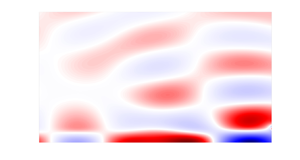
Examples of the normalised pressure eigenfunctions of the waves upstream and downstream of the shock are reported in figure 7. For the V-S (figure 7a), the incident and transmitted K–H waves show a peak at the V-S location and the reflected waves, that is  $k_p^-$ and $k_a^-$ modes, have support both inside and outside the jet. We note that, although there is no energy loss at $r=r_{MAX}$ as a consequence of the imposition of a soft-wall boundary condition, the energy of $k_a$ modes reflected back cannot be transferred to the other discrete modes since the flow is locally parallel. On the transmitted side downstream of the shock, while the evanescent $k_p^+$ wave with $n_r=1$ has a support both in the inner and outer part of the jet, the transmitted $k_p^+$ modes with $n_r>1$ show a spatial support concentrated inside the jet, consistent with their identity as acoustic waves trapped within the jet core. Examples of the pressure eigenfunctions of the waves upstream and downstream of the shock computed using the F-T model are shown in figure 7(b). The incident K–H mode and the reflected $k_p^-$ and $k_a^-$ have a similar shape to that found using the V-S model. As mentioned above, $k_{cr}^+$ modes have eigenfunctions with a spatial support concentrated either inside of the jet or in the shear layer depending on the wavenumber value considered. The spatial support of the critical-layer modes moves to larger $r$ and the phase velocity $U_{\phi }$ decreases as $\vert k_{cr}\vert$ increases.
Pressure eigenfunctions for  $m=0$ and $St=0.68$ computed using (a) the V-S model and (b) the F-T model. The colours are the same as those used in figures 3, 4, 5 and 6 to identify the different mode families upstream and downstream of the shock, respectively. (i) Incident and reflected waves upstream of the shock for $M_j=1.1$ and $T\approx 0.81$: solid blue line refers to the incident $k_{KH}^+$ wave, dashed red line to the propagative $k_p^-$ wave with $n_r=2$, dotted black line to the evanescent $k_p^-$ mode with $n_r=1$, dash-dotted magenta line to the propagative $k_a^-$ wave. (ii) Transmitted waves downstream of the shock for $M_{j_2}=0.91$ and $T\approx 0.85$: solid blue line refers to the transmitted $k_{KH}^+$ mode, dotted black line to the evanescent $k_p^+$ with $n_r=1$, dashed green line to the evanescent $k_p^+$ with $n_r=2$, dash-dotted magenta line to the propagative $k_a^+$ wave, solid and bold cyan lines to $k_{cr}^+$ modes.

3.2. Reflection coefficient
Second, we present the reflection-coefficient values calculated by minimising the error objective function  $F$ in (2.8) via the pseudo-inverse solution (2.12). Figure 8 shows the evolution of the objective function $F$ as a function of the number of reflected and transmitted modes $n=n_R+n_T$ for both the V-S and F-T models. Here, $F$ is normalised so as to have unitary value when the sole incident K–H wave is considered in the minimisation algorithm, thus allowing us to quantify the relevance of the modes added in the computation in terms of error reduction. We here make a convergence analysis showing how the objective function changes by adding reflected and transmitted modes. In the absence of any unquestionable criterion allowing us to know a priori the relevance of each mode in the reflection/transmission dynamics, we choose to add modes as a function of the family they belong to. For each mode family, waves are added by increasing $\vert k\vert$. Specifically, we first add in the calculation the reflected waves, that is the $k_p^-$ and $k_a^-$ mode families, and then we add the transmitted modes downstream of the shock, that is $k_{KH}^+$ and its complex conjugate, the $k_p^+$ modes for $n_r\geq 1$, the $k_a^+$ modes and the $k_{cr}^+$ waves in the case of the F-T model, for a total number of modes $N=N_R+N_T=800$. The final results are independent of the mode arrangement. The objective function remains approximately constant when reflected waves are added. The transmitted K–H mode provides a significant decay in the cost function, which indicates that it has an important role in the reflection/transmission mechanism, as the impinging and transmitted K–H modes have a similar structure. For the V-S, the addition of the other transmitted modes has a small impact on the cost functional, which saturates at a value of ${\approx }10^{-2}$. On the contrary, for the F-T model, the addition of critical-layer modes produces an important reduction of the cost function, which saturates at a value of $5\times 10^{-3}$, lower than that observed in the case of the V-S.

Figure 9 shows the evolution of the amplitude and phase of the reflection coefficient associated with the upstream-travelling guided mode of second radial order as a function of the number of modes  $n$ obtained using the V-S model. On the reflected side, the significant drop of $\vert R\vert$ observed when $k_a^-$ modes are added is due to propagative acoustic modes. Similar to the objective function in figure 8(a), both the amplitude and phase of the reflection coefficient undergo a significant jump when modes on the transmitted side are included in the calculation. Specifically, the solution does not drastically change after the inclusion of the $k_{KH}^+$ mode and remains approximately constant. The solution converges to $5.8\times 10^{-3}$ and $-0.38$ for the amplitude and phase, respectively.
Evolution of the reflection coefficient computed using the V-S as a function of the modes considered in the calculation (markers and colours are the same as those used to identify the modes in the eigenspectra in figures 3 and 5): (a) amplitude, (b) phase. Blue dotted lines indicate  $\pm {\rm \pi}$ in the phase plot.

The evolution of the amplitude and phase of the reflection coefficient as a function of  $n$ in the case of the F-T model is shown in figure 10. Similar to the V-S model, we see a significant change in the value of both amplitude and phase when modes on the transmitted side are included in the calculation. Consistent with what we observed in the objective function trend, the addition of the $k_{cr}^+$ modes plays an important role in the determination of the reflection coefficient. Specifically, a significant drop in amplitude occurs for critical-layer modes with $5.5\leq \vert k\vert \leq 21$, after which both the amplitude and phase values remain approximately constant. These are modes with wavelength in the range $\approx [0.3D,D]$ and, hence, 6 to 20 times the shear-layer thickness. Their phase speed is $\approx$ $0.2U_j\leq U_{\phi }\leq 0.75U_j$, and they are mostly concentrated in the centre of the shear layer, as shown in figure 11.
Evolution of the amplitude and phase of the reflection coefficient computed using the F-T model as a function of the number of modes considered. Markers and colours are the same as those used in figures 4 and 6 to identify the mode families. (a) amplitude, (b) phase. Blue dotted lines indicate  $\pm {\rm \pi}$ in the phase plot.

Normalised eigenfunctions of  $k_{cr}^+$ modes computed using the F-T model as a function of wavenumber $k$ and radial distance $r$: (a) pressure, (b) axial velocity, (c) radial velocity.

A summary of the reflection-coefficient values obtained for both flow models is reported in table 2. A large discrepancy between the V-S and F-T model is found for both the amplitude and phase of the reflection coefficient. This result suggests that the presence of a finite thickness and the associated shear-layer dynamics, which cannot be described using a vortex sheet, plays an important role in the reflection/transmission mechanism and needs to be taken into account to perform a reliable estimation of the reflection coefficient.
Summary of the reflection-coefficient values associated with the upstream-travelling guided mode of second radial order generated by the interaction between an incident K–H wave on a shock. Results obtained using both the V-S and F-T models to describe the jet dynamics are reported.

3.2.1. Reflected and transmitted pressure fields
The reflected and transmitted pressure fields for the flow condition investigated above using a F-T model are here reconstructed in the  $x$–
$x$– $r$ plane. Using the normal-mode ansatz (2.4), the reflected and transmitted fields are given by
 $$\begin{gather} p_R\left(x,r,\theta\right)=\sum_{n_R=1}^{N_R}R_{n_R} \hat{p}_{1R,n_R}\exp({{\rm i}\left(k_{nR}x+m\theta\right)}), \end{gather}$$
 $$\begin{gather}p_T\left(x,r,\theta\right)=\sum_{n_T=1}^{N_T}T_{n_T} \hat{p}_{2T,n_T}\exp({{\rm i}\left(k_{nT}x+m\theta\right)}). \end{gather}$$
 We set  $x=0$ to be the location of the shock discontinuity, so the reflected upstream-travelling and transmitted downstream-travelling waves evolve along negative and positive $x$ directions, respectively. Figure 12 shows the entire reflected field as well as the reflected fields for each type of the upstream-travelling modes considered in the reflection-coefficient calculation, that is the propagative $k_p^-$ mode with $n_r=2$, the evanescent $k_p^-$ mode with $n_r=1$ and an example of the propagative and evanescent $k_a^-$ waves with $\vert k\vert \approx 2.79$ and $2.1$, respectively. The fields reconstructed using the $k_p^-$ modes show a spatial support both inside and outside the jet with a prescribed radial decay. Regarding the axial evolution, the evanescent $k_p^-$ mode with $n_r=1$ exhibits a decay starting from the shock position $x=0$, whereas the $k_p^-$ mode with $n_r=2$ has a fixed axial structure consistent with its neutrally stable nature. A similar behaviour is found for the pressure fields reconstructed using propagative and evanescent free-stream acoustic waves. The entire reflected pressure field, which results from the linear superposition of all the reflected $k^-$ waves, shows an axially and radially decaying structure starting from $x=0$ and $r=0$, respectively.
Reconstruction of the reflected fields in the  $x-r$ plane for a shock discontinuity located at $x=0$: (a) $k_p^-$ mode with $n_r=2$, (b) $k_p^-$ mode with $n_r=1$, (c) propagative $k_a^-$ wave, (d) evanescent $k_a^-$ wave, (e) total field.

The entire transmitted field as well as the transmitted fields for each mode family considered in the reflection-coefficient calculation are shown in figure 13. We here report the fields obtained using the  $k_{KH}^+$ wave, the evanescent supersonic $k_p^+$ mode with $n_r=1$, the evanescent subsonic $k_p^+$ mode with $n_r=2$, the propagative and evanescent $k_a^+$ waves with $\vert k\vert \approx 2.7$ and $2.8$, respectively, and the $k_{cr}^+$ mode for $\vert k\vert \approx 11.5$. Consistent with its unstable nature, the shape and intensity of the total transmitted field is dominated by the K–H mode. The shape of the transmitted fields reconstructed using the individual mode family is consistent with the neutral/evanescent nature and radial structure described above.
Reconstruction of the transmitted fields in the  $x$–
$x$– $r$ plane for a shock discontinuity located at $x=0$: (a) $k_{KH}^+$ wave, (b) supersonic $k_p^-$ mode with $n_r=1$, (c) subsonic $k_p^+$ with $n_r=2$, (d) propagative $k_a^+$ wave, (e) evanescent $k_a^+$ wave, ( f) $k_{cr}^+$ mode, (g) total field.

3.2.2. Frequency–Mach-number dependence of the reflection coefficient
We here explore the frequency–Mach-number dependence of the reflection coefficient associated with the upstream-travelling guided mode with  $n_r=2$ obtained using the F-T model. For this purpose, we let the jet Mach number vary in the range $M_j=[1,1.7]$ and explore the Strouhal-number band for which the guided mode is propagative for such flow conditions, that is the $St$-number range delimited by the branch and saddle points (see Mancinelli et al. Reference Mancinelli, Jaunet, Jordan and Towne2019a, Reference Mancinelli, Jaunet, Jordan and Towne2021). The resolutions for ${\rm \Delta} M_j$ and ${\rm \Delta} St$ were set equal to $10^{-2}$ and $5\times 10^{-3}$, respectively. Figure 14 shows the evolution of the normalised objective function $F$ as a function of $M_j$ and $St$. The errors are very small for low $M_j$ and gradually rise as the jet Mach number increases but never exceed 13 %. The amplitude and the phase modulus of the reflection coefficient as a function of $St$ and $M_j$ are shown in figure 15. The reflection-coefficient amplitude rises with increasing $M_j$ for a given $St$ and appears to be larger in the proximity of the saddle point for all $M_j$, with the jet-flow region $M_j=[1.17,1.37]$ showing the highest amplitude. Overall, the phase gradually increases for larger $M_j$ and lower $St$. We note that a jump from in-phase to out-of-phase conditions is found for $M_j=1.58$ for most frequencies.
Normalised error objective function as a function of Strouhal and jet Mach numbers for the F-T model. Dashed and dash-dotted lines refer to the branch- and saddle-point locations, respectively.

Evolution of the reflection coefficient as a function of Strouhal and jet Mach numbers for the F-T model. Dashed and dash-dotted lines refer to the branch- and saddle-point locations, respectively. (a) Amplitude, (b) phase.

4. Conclusions
The scattering of a K–H wave into a discrete, upstream-travelling guided mode due to a normal shock in a jet flow was computed in the present manuscript. Jets with zero-thickness and F-T shear layers were modelled with an analytical V-S and a numerical solution of the Rayleigh equation, respectively. The reflection coefficient associated with the scattered, upstream-travelling wave was calculated via a mode-matching technique enforcing conservation equations through the shock discontinuity. Assuming small disturbances, the shock equations were linearised about the mean flow and the possible scattered modes, i.e. upstream-travelling reflected waves and downstream-travelling transmitted waves, were identified by assessing the corresponding group velocity using the Briggs–Bers criteria. Solutions based on a truncated set of modes were obtained via the minimisation of the error in the conservation equations, which corresponds to a weighted pseudo-inverse solution. The F-T model showed that critical-layer modes, characterised by eigenfunctions with radial support mostly concentrated in the centre of the shear layer, by a wavelength 6 to 20 times the shear-layer thickness and by a phase velocity between 0.2 and 0.75 of the jet velocity, play an important role in the reflection-coefficient calculation and, thus, most likely in the physical mechanisms underpinning the process. The reconstructed reflected and transmitted pressure fields in the  $x$–
$x$– $r$ plane showed an organised structure consistent with the axial and radial evolution of the modes calculated by the F-T model. The frequency–Mach-number dependence of the reflection coefficient has been explored, revealing that the reflection-coefficient amplitude is larger for frequencies in the proximity of the saddle point and for jet Mach-number values in between 1.17 and 1.37. The phase exhibited a gradual increase as the Strouhal and jet Mach numbers decreased and increased, respectively.
The mode-matching approach described in this paper appears to be a relevant and promising tool for better describing and predicting resonant dynamics found in jets, such as screech in supersonic jets. A similar approach may be developed to evaluate the reflection coefficient at the nozzle exit, thus providing all the elements to make screech-frequency predictions without any input from data using the model presented in Mancinelli et al. (Reference Mancinelli, Jaunet, Jordan and Towne2021).
Acknowledgements
The authors acknowledge the financial support of EU and Nouvelle-Acquitaine region under the program CPER-FEDER. M.M. acknowledges the support of Centre National d’Études Spatiales (CNES) under a post-doctoral grant at the time of the writing of the paper. E.M. acknowledges the financial support of Commissariat à l'Energie Atomique, Centre d'Etudes Scientifiques et Techniques d'Aquitaine (CEA-CESTA) under a post-doctoral grant.
Declaration of interests
The authors report no conflict of interest.
Appendix A. Linearised Euler equations
The non-dimensional Euler equations in cylindrical coordinates are
 \begin{gather}\left.\begin{aligned}
&\dfrac{{\rm D}\rho}{{\rm D} t}+\rho\boldsymbol{\nabla}\boldsymbol{\cdot}\boldsymbol{u}=0,\\
&\rho\dfrac{{\rm D} u_x}{{\rm D} t}=-\dfrac{\partial p}{\partial x},\\
&\rho\left(\dfrac{{\rm D} u_r}{{\rm D} t}-\dfrac{u_\theta^2}{r}\right)=-\dfrac{\partial p}{\partial r},\\
&\rho\left(\dfrac{{\rm D} u_\theta}{{\rm D} t}+\dfrac{u_ru_\theta}{r}\right)=-\dfrac{1}{r}\dfrac{\partial p}{\partial \theta},\\
&\dfrac{{\rm D} T}{{\rm D} t}+\left(\gamma -1\right)T\boldsymbol{\nabla}\boldsymbol{\cdot}\boldsymbol{u}=0,\\
&p=\dfrac{\gamma - 1}{\gamma}\rho T,
\end{aligned}\right\}
\end{gather}
\begin{gather}\left.\begin{aligned}
&\dfrac{{\rm D}\rho}{{\rm D} t}+\rho\boldsymbol{\nabla}\boldsymbol{\cdot}\boldsymbol{u}=0,\\
&\rho\dfrac{{\rm D} u_x}{{\rm D} t}=-\dfrac{\partial p}{\partial x},\\
&\rho\left(\dfrac{{\rm D} u_r}{{\rm D} t}-\dfrac{u_\theta^2}{r}\right)=-\dfrac{\partial p}{\partial r},\\
&\rho\left(\dfrac{{\rm D} u_\theta}{{\rm D} t}+\dfrac{u_ru_\theta}{r}\right)=-\dfrac{1}{r}\dfrac{\partial p}{\partial \theta},\\
&\dfrac{{\rm D} T}{{\rm D} t}+\left(\gamma -1\right)T\boldsymbol{\nabla}\boldsymbol{\cdot}\boldsymbol{u}=0,\\
&p=\dfrac{\gamma - 1}{\gamma}\rho T,
\end{aligned}\right\}
\end{gather}
where
 $$\begin{gather} \frac{{\rm D}}{{\rm D} t}=\frac{\partial}{\partial t}+u_x\frac{\partial}{\partial x}+u_r\frac{\partial}{\partial r}+\frac{u_\theta}{r}\frac{\partial}{\partial\theta}, \end{gather}$$
 $$\begin{gather}\boldsymbol{\nabla}\boldsymbol{\cdot}\boldsymbol{u}=\frac{\partial u_x}{\partial x}+\frac{\partial u_r}{\partial r}+\frac{u_r}{r}+\frac{1}{r}\frac{\partial u_\theta}{\partial \theta}. \end{gather}$$
Inserting the Reynolds decomposition (2.2), removing the mean and linearising, the LEE are written
 \begin{gather}\left.\begin{aligned}
&\dfrac{\partial\rho}{\partial t}+\bar{u}_x\dfrac{\partial\rho}{\partial x}+u_r\dfrac{\partial\bar{\rho}}{\partial r}+\bar{\rho}\left(\dfrac{\partial u_x}{\partial x}+
\dfrac{\partial u_r}{\partial r}+\dfrac{u_r}{r}+\dfrac{1}{r}\dfrac{\partial u_\theta}{\partial\theta}\right)=0,\\
&\bar{\rho}\left(\dfrac{\partial u_x}{\partial t}+\bar{u}_x\dfrac{\partial u_x}{\partial x}+u_r\dfrac{\partial\bar{u}_x}{\partial r}\right)=-\dfrac{\partial p}{\partial x},\\
&\bar{\rho}\left(\dfrac{\partial u_r}{\partial t}+\bar{u}_x\dfrac{\partial u_r}{\partial x}\right)=-\dfrac{\partial p}{\partial r},\\
&\bar{\rho}\left(\dfrac{\partial u_\theta}{\partial t}+\bar{u}_x\dfrac{\partial u_\theta}{\partial x}\right)=-\dfrac{1}{r}\dfrac{\partial p}{\partial \theta},\\
&\dfrac{\partial T}{\partial t}+\bar{u}_x\dfrac{\partial T}{\partial x}+u_r\dfrac{\partial \bar{T}}{\partial r}+\left(\gamma -1\right)\bar{T}\left(\dfrac{\partial u_x}{\partial x}+
\dfrac{\partial u_r}{\partial r}+\dfrac{u_r}{r}+\dfrac{1}{r}\dfrac{\partial u_\theta}{\partial\theta}\right)=0,\\
&p=\dfrac{\gamma -1}{\gamma}\left(\bar{\rho}T+\bar{T}\rho\right),
\end{aligned}\right\}
\end{gather}
\begin{gather}\left.\begin{aligned}
&\dfrac{\partial\rho}{\partial t}+\bar{u}_x\dfrac{\partial\rho}{\partial x}+u_r\dfrac{\partial\bar{\rho}}{\partial r}+\bar{\rho}\left(\dfrac{\partial u_x}{\partial x}+
\dfrac{\partial u_r}{\partial r}+\dfrac{u_r}{r}+\dfrac{1}{r}\dfrac{\partial u_\theta}{\partial\theta}\right)=0,\\
&\bar{\rho}\left(\dfrac{\partial u_x}{\partial t}+\bar{u}_x\dfrac{\partial u_x}{\partial x}+u_r\dfrac{\partial\bar{u}_x}{\partial r}\right)=-\dfrac{\partial p}{\partial x},\\
&\bar{\rho}\left(\dfrac{\partial u_r}{\partial t}+\bar{u}_x\dfrac{\partial u_r}{\partial x}\right)=-\dfrac{\partial p}{\partial r},\\
&\bar{\rho}\left(\dfrac{\partial u_\theta}{\partial t}+\bar{u}_x\dfrac{\partial u_\theta}{\partial x}\right)=-\dfrac{1}{r}\dfrac{\partial p}{\partial \theta},\\
&\dfrac{\partial T}{\partial t}+\bar{u}_x\dfrac{\partial T}{\partial x}+u_r\dfrac{\partial \bar{T}}{\partial r}+\left(\gamma -1\right)\bar{T}\left(\dfrac{\partial u_x}{\partial x}+
\dfrac{\partial u_r}{\partial r}+\dfrac{u_r}{r}+\dfrac{1}{r}\dfrac{\partial u_\theta}{\partial\theta}\right)=0,\\
&p=\dfrac{\gamma -1}{\gamma}\left(\bar{\rho}T+\bar{T}\rho\right),
\end{aligned}\right\}
\end{gather}
where we removed the primes from the fluctuating variables for notational simplicity. The locally parallel-flow assumption implies that the derivatives along the axial and azimuthal directions  $x$ and $\theta$ are zero as well as the mean radial and azimuthal velocities $\bar {u}_r$ and $\bar {u}_\theta$. Assuming the normal-mode ansatz (2.4) yields
 \begin{gather}\left.\begin{aligned}
&-{\rm i}\omega\hat{\rho}+\bar{u}_x{\rm i}k\hat{\rho}+\dfrac{\partial\bar{\rho}}{\partial r}\hat{u}_r+\bar{\rho}\left({\rm
i}k\hat{u}_x+ \dfrac{\partial\hat{u}_r}{\partial r}+\dfrac{\hat{u}_r}{r}+\dfrac{{\rm i}m}{r}\widehat{u_\theta}\right)=0,\\
&\bar{\rho}\left(-{\rm i}\omega\hat{u}_x+\bar{u}_x{\rm i}k\hat{u}_x+\dfrac{\partial\bar{u}_x}{\partial r}\hat{u}_r\right)=-{\rm i}k\hat{p},\\
&\bar{\rho}\left(-{\rm i}\omega\hat{u}_r+\bar{u}_x{\rm i}k\hat{u}_r\right)=-\dfrac{\partial\hat{p}}{\partial r},\\
&\bar{\rho}\left(-{\rm i}\omega\hat{u}_\theta+\bar{u}_x{\rm i}k\hat{u}_\theta\right)=-\dfrac{{\rm i}m}{r}\hat{p},\\
&-{\rm i}\omega\hat{T}_+\bar{u}_x{\rm i}k\hat{T}+\dfrac{\partial\bar{T}}{\partial r}\hat{u}_r+\left(\gamma -1\right)
\bar{T}\left({\rm i}k\hat{u}_x+\dfrac{\partial\hat{u}_r}{\partial r}+\dfrac{\hat{u}_r}{r}+\dfrac{{\rm i}m}{r}\widehat{u_\theta}\right)=0,\\
&\hat{p}=\dfrac{\gamma-1}{\gamma}\left(\bar{\rho}\hat{T}+\bar{T}\hat{\rho}\right).
\end{aligned}\right\}
\end{gather}
\begin{gather}\left.\begin{aligned}
&-{\rm i}\omega\hat{\rho}+\bar{u}_x{\rm i}k\hat{\rho}+\dfrac{\partial\bar{\rho}}{\partial r}\hat{u}_r+\bar{\rho}\left({\rm
i}k\hat{u}_x+ \dfrac{\partial\hat{u}_r}{\partial r}+\dfrac{\hat{u}_r}{r}+\dfrac{{\rm i}m}{r}\widehat{u_\theta}\right)=0,\\
&\bar{\rho}\left(-{\rm i}\omega\hat{u}_x+\bar{u}_x{\rm i}k\hat{u}_x+\dfrac{\partial\bar{u}_x}{\partial r}\hat{u}_r\right)=-{\rm i}k\hat{p},\\
&\bar{\rho}\left(-{\rm i}\omega\hat{u}_r+\bar{u}_x{\rm i}k\hat{u}_r\right)=-\dfrac{\partial\hat{p}}{\partial r},\\
&\bar{\rho}\left(-{\rm i}\omega\hat{u}_\theta+\bar{u}_x{\rm i}k\hat{u}_\theta\right)=-\dfrac{{\rm i}m}{r}\hat{p},\\
&-{\rm i}\omega\hat{T}_+\bar{u}_x{\rm i}k\hat{T}+\dfrac{\partial\bar{T}}{\partial r}\hat{u}_r+\left(\gamma -1\right)
\bar{T}\left({\rm i}k\hat{u}_x+\dfrac{\partial\hat{u}_r}{\partial r}+\dfrac{\hat{u}_r}{r}+\dfrac{{\rm i}m}{r}\widehat{u_\theta}\right)=0,\\
&\hat{p}=\dfrac{\gamma-1}{\gamma}\left(\bar{\rho}\hat{T}+\bar{T}\hat{\rho}\right).
\end{aligned}\right\}
\end{gather}
The Fourier-transformed LEE (A4f) can be written exclusively in terms of pressure, leading to the compressible Rayleigh equation (2.13). The eigenfunctions  $\hat {u}_i(r)$, $\hat {\rho }(r)$ and $\hat {T}(r)$ are recovered from the pressure
 $$\begin{gather} \hat{u}_x\left(r\right)={-}\frac{1}{\bar{\rho} \left(\bar{u}_xk-\omega\right)^2}\frac{\partial\bar{u}_x}{\partial r} \frac{\partial\hat{p}}{\partial r}-\frac{k}{\bar{\rho}\left(\bar{u}_xk-\omega\right)}\hat{p}, \end{gather}$$
 $$\begin{gather}\hat{u}_r\left(r\right)={-}\frac{1}{\bar{\rho}\left(\bar{u}_x{\rm i}k-{\rm i}\omega\right)} \frac{\partial\hat{p}}{\partial r}, \end{gather}$$
 $$\begin{gather}\hat{u}_\theta\left(r\right)={-}\frac{m}{\bar{\rho}r\left(\bar{u}_xk-\omega\right)}\hat{p}, \end{gather}$$
 $$\begin{gather}\hat{\rho}\left(r\right)={-}\frac{1}{\left(\bar{u}_xk-\omega\right)^2} \left(\frac{\partial^2\hat{p}}{\partial r^2}+\left(\frac{1}{r}-\frac{2k}{\bar{u}_xk-\omega} \frac{\partial\bar{u}_x}{\partial r}\right) \frac{\partial\hat{p}}{\partial r}-\left(k^2+\frac{m^2}{r^2}\right)\hat{p}\right), \end{gather}$$
 \begin{gather} \hat{T}\left(r\right)={-}\frac{\left(\gamma -1\right)\bar{T}}{\bar{\rho}\left(\bar{u}_xk-\omega\right)^2} \left(\frac{\partial^2\hat{p}}{\partial r^2}+\left(\frac{1}{r}-\frac{2k}{\bar{u}_xk-\omega}\frac{\partial\bar{u}_x}{\partial r}-\frac{1}{\bar{\rho}}\frac{\partial\bar{\rho}}{\partial r}+\frac{1}{\left(\gamma -1\right)\bar{T}}\frac{\partial\bar{T}}{\partial r}\right)\frac{\partial\hat{p}}{\partial r} \right.\nonumber\\ \left. -\left(k^2+\frac{m^2}{r^2}\right)\hat{p}\right). \end{gather}
Appendix B. Energy norm derivation
Eigenfunctions are normalised to have zero phase for the pressure eigenfunction on the centreline and to have unitary energy norm. Following Chu (Reference Chu1965), the energy norm is defined as
 \begin{equation} E=\frac{1}{2}\int_V\left(A u_i^*u_i + B\rho^*\rho+C T^*T\right)\mathrm{d}V, \end{equation}
where the  $*$ indicates the complex conjugate and the constants $A$,
$A$,  $B$ and $C$ have to determined on the basis of the flow considered (Hanifi et al. Reference Hanifi, Schmid and Henningson1996). We assume a medium at rest, thus implying $\bar {u}_x=0$ and $\partial \bar {q}/\partial r=0$. Hence, the LEE reduce to the following:
 \begin{gather}\left.\begin{aligned}
&\frac{\partial\rho}{\partial t}+\bar{\rho}\boldsymbol{\nabla}\boldsymbol{\cdot}\boldsymbol{u}=0,\\
&\bar{\rho}\frac{\partial u_x}{\partial t}=-\frac{\partial p}{\partial x},\\
&\bar{\rho}\frac{\partial u_r}{\partial t}=-\frac{\partial p}{\partial r},\\
&\bar{\rho}\frac{\partial u_\theta}{\partial t}=-\frac{1}{r}\frac{\partial p}{\partial \theta},\\
&\frac{\partial T}{\partial t}+\left(\gamma -1\right)\bar{T}\boldsymbol{\nabla}\boldsymbol{\cdot}\boldsymbol{u}=0,\\
&p=\frac{\gamma-1}{\gamma}\left(\bar{\rho}T+\bar{T}\rho\right),
\end{aligned}\right\}
\end{gather}
\begin{gather}\left.\begin{aligned}
&\frac{\partial\rho}{\partial t}+\bar{\rho}\boldsymbol{\nabla}\boldsymbol{\cdot}\boldsymbol{u}=0,\\
&\bar{\rho}\frac{\partial u_x}{\partial t}=-\frac{\partial p}{\partial x},\\
&\bar{\rho}\frac{\partial u_r}{\partial t}=-\frac{\partial p}{\partial r},\\
&\bar{\rho}\frac{\partial u_\theta}{\partial t}=-\frac{1}{r}\frac{\partial p}{\partial \theta},\\
&\frac{\partial T}{\partial t}+\left(\gamma -1\right)\bar{T}\boldsymbol{\nabla}\boldsymbol{\cdot}\boldsymbol{u}=0,\\
&p=\frac{\gamma-1}{\gamma}\left(\bar{\rho}T+\bar{T}\rho\right),
\end{aligned}\right\}
\end{gather}
where we have removed the prime for the fluctuating part for notational simplicity. We calculate the time evolution of the energy norm
 \begin{equation} \frac{\partial E}{\partial t}=\frac{\partial E}{\partial u_i} \frac{\partial u_i}{\partial t} + \frac{\partial E}{\partial \rho} \frac{\partial \rho}{\partial t} + \frac{\partial E}{\partial T}\frac{\partial T}{\partial t}, \end{equation}
which, exploiting (B2a), can be written as
 \begin{equation} \frac{\partial E}{\partial t}={-}\frac{1}{2}\int_V \left(A u_i\frac{1}{\bar{\rho}}\boldsymbol{\nabla} p + B\rho \bar{\rho}\boldsymbol{\nabla}\boldsymbol{\cdot} \boldsymbol{u} + CT\left(\gamma -1\right)\bar{T}\boldsymbol{\nabla}\boldsymbol{\cdot}\boldsymbol{u}\right)\mathrm{d}V. \end{equation}
 Expressing  $\rho =({\gamma }/{\gamma -1})({p}/{\bar {T}})-({\bar {\rho }}/{\bar {T}})T$ from (B2f) and applying integration by parts on the first term on the right-hand side of (B4), the time evolution of the energy norm becomes
 \begin{gather} \frac{\partial E}{\partial t}={-}\int_{\partial V}u_ip\,\mathrm{d}S + \int_V \left(\frac{A}{\bar{\rho}}p - B\bar{\rho}\left(\frac{\gamma}{\gamma -1} \frac{p}{\bar{T}}-\frac{\bar{\rho}}{\bar{T}}T\right) - CT\left(\gamma -1\right)\bar{T}\right) \boldsymbol{\nabla}\boldsymbol{\cdot}\boldsymbol{u}\,\mathrm{d}V, \end{gather}
where  $\int _{\partial V}u_ip\,\mathrm {d}S$ represents the acoustic power crossing the domain $V$. Hence, $\partial E/\partial t+\int _{\partial V}u_ip\,\mathrm {d}S$ can be interpreted as the total energy variation, which we impose to be conservative thus leading to the following expression:
 \begin{equation} \int_V \left(\frac{A}{\bar{\rho}} - B\frac{\bar{\rho}}{\bar{T}} \frac{\gamma}{\gamma -1}\right)p\boldsymbol{\nabla}\boldsymbol{\cdot}\boldsymbol{u}\,\mathrm{d}V + \int_V \left(B\frac{\bar{\rho}^2}{\bar{T}} - C\left(\gamma -1\right)\bar{T}\right)T\boldsymbol{\nabla}\boldsymbol{\cdot}\boldsymbol{u}\,\mathrm{d}V = 0. \end{equation}
Equation (B6) can be equal to zero if and only if
 \begin{gather}\left.\begin{aligned} &\frac{A}{\bar{\rho}} - B\frac{\bar{\rho}}{\bar{T}}\frac{\gamma}{\gamma -1}=0,\\ &B\frac{\bar{\rho}^2}{\bar{T}} - C\left(\gamma -1\right)\bar{T}=0. \end{aligned}\right\} \end{gather}
 By legitimately imposing  $A=\bar {\rho }$, it is straightforward to calculate the values for the other two constants
 \begin{gather}\left.\begin{aligned} B&=\frac{\gamma -1}{\gamma}\frac{\bar{T}}{\bar{\rho}},\\ C&=\frac{\bar{\rho}}{\gamma\bar{T}}. \end{aligned}\right\} \end{gather}
For an inviscid locally parallel flow with medium at rest, the energy norm is finally given by (2.14).
Appendix C. Mean radial velocity downstream of the shock
The presence of the shock wave generates a mean pressure gradient along the radial direction downstream of the shock. This induces the appearance of a mean radial velocity. This radial velocity is here evaluated in the case of a finite thickness model in order to establish that it does not affect the calculation of the reflection coefficient. We consider the momentum equation along the radial direction (A1c). The conservation equation for the mean flow is
 \begin{equation} \bar{\rho}\bar{u}_r\frac{\partial\bar{u}_r}{\partial r}={-}\frac{\partial\bar{p}}{\partial r}, \end{equation}
which gives for the mean radial velocity the following expression:
 \begin{equation} \bar{u}_r=\sqrt{-2\int_0^\infty\frac{1}{\bar{\rho}}\frac{\partial\bar{p}}{\partial r}\mathrm{d}r}. \end{equation}
 The radial derivative is computed using a centred finite-difference method. The radial profile of the mean radial velocity normalised by the jet Mach number downstream of the shock is reported in figure 16. We note that  $\bar {u}_r\neq 0$ in the shear-layer region with a peak for $r=0.5$. Nevertheless, since the maximum value is approximately 10 % of the jet velocity, we may assert that the jet is slowly diverging downstream of the shock, but this feature does not affect the evaluation of the reflection coefficient given that both the reflection and transmission mechanisms happen locally and are not influenced by the flow evolution far away from the shock.
Mean radial velocity profile along the radial direction downstream of the shock for  $M_{j_1}$ and $M_{j_2}$ equal to 1.1 and 0.91, respectively.

Appendix D. Relevance of the near-sonic, downstream-travelling acoustic modes
As outlined in Mancinelli et al. (Reference Mancinelli, Martini, Jaunet and Jordan2022), propagative, downstream-travelling acoustic modes in the vicinity of the sonic line cannot be described using the confined V-S model due to numerical issues in the root-finder algorithm when searching for zeros of the dispersion relation. Furthermore, the resolution of the acoustic branch close to the sonic line is function of the distance of the wall boundary  $r_{MAX}$, as exemplified in figure 17, which shows the maximum value of the acoustic eigenvalue of the propagative, downstream-travelling branch as a function of $r_{MAX}$. The resolution in the vicinity of the sonic line deteriorates for increasing $r_{MAX}$, thus bringing into question the reliability of the results obtained using the V-S. To prove the little relevance of near-sonic, downstream-travelling acoustic modes in the determination of the reflection coefficient we consider the F-T model and compute $R$ both including and excluding near-sonic modes. The comparison in figure 18 shows no discrepancy in terms of both amplitude and phase when near-sonic acoustic modes are artificially removed from the reduced basis of the transmitted modes, thus suggesting the small influence of these modes in the reflection coefficient calculation and confirming the reliability of the results obtained using the V-S. To further support this assertion, we finally show in figure 19 the variation of the objective function $F$, the reflection-coefficient amplitude and phase as a function of $r_{MAX}$ when using the V-S to describe the jet dynamics. The variation is relative to the results obtained using $r_{MAX}=100$ and presented throughout the manuscript. We observe variation lower than 0.1 % for the objective function and of the order of 10 % and 7 % at maximum for the reflection-coefficient amplitude and phase, respectively. These variations are considered acceptable especially given that, as outlined by Mancinelli et al. (Reference Mancinelli, Martini, Jaunet and Jordan2022), the change of $r_{MAX}$ implies a change of the discretisation of the acoustic branch and, hence, of the number of modes considered in the calculation of the reflection coefficient.
Maximum eigenvalue of the propagative, downstream-travelling acoustic branch as a function of the wall distance using the confined V-S model. Flow conditions are the same reported in figure 5 downstream of the shock. Blue  $\circ$ represent the eigenvalue, dashed red line the position of the sonic line.

Evolution of the reflection coefficient as a function of the number of modes considered using the F-T model: blue  $\diamond$ refer to results obtained including near-sonic, downstream-travelling acoustic modes, red $\circ$ refer to results obtained artificially removing near-sonic acoustic modes ( $k_{a_{MAX}}^+=3.2$). (a) Amplitude, (b) phase.

Variation of the objective function, amplitude and phase of the reflection coefficient as a function of the wall distance using the confined V-S model. Variations are relative to the results obtained for  $r_{MAX}=100$ presented throughout the manuscript. (a) Objective function, (b) reflection-coefficient amplitude, (c) reflection-coefficient phase.


 Open access