


1. Introduction
Water-wave propagation and scattering near menisci occur in diverse natural, laboratory and engineered settings. These menisci form around structures like plant stems, floating debris and aquatic insects, altering local wave generation and transmission. Consequently, meniscus-modified wave scattering influences small-scale fluid processes ranging from aquatic insect communication via ripples (Wilcox Reference Wilcox1995) and water-strider locomotion (Hu, Chan & Bush Reference Hu, Chan and Bush2003) to droplet manipulation (Tran et al. Reference Tran, Byun, Nguyen and Kang2009), thin-film transport (Tsuda et al. Reference Tsuda, de, Juan and Scriven2010), fluid motion in open channels (Tokihiro et al. Reference Tokihiro, Tu, Berthier, Lee, Dostie, Khor, Eakman, Theberge and Berthier2023) and aquatic robots (Tarr et al. Reference Tarr, Brunner, Soto and Goldman2024). Meniscus effects have been studied in relation to travelling-wave speed and wave sloshing parameters, including frequency, damping and instability threshold (Scott & Benjamin Reference Scott and Benjamin1978; Benjamin & Scott Reference Benjamin and Scott1979; Miles Reference Miles1990, Reference Miles1992; Perlin & Schultz Reference Perlin and Schultz2000; Kidambi & Shankar Reference Kidambi and Shankar2004; Nicolás Reference Nicolás2005; Kidambi Reference Kidambi2009; Nguyem Thu Lam & Caps Reference Nguyem Thu Lam and Caps2011; Shao et al. Reference Shao, Gabbard, Bostwick and Saylor2021; Monsalve et al. Reference Monsalve, Maurel, Pagneux and Petitjeans2022). However, their specific influence on surface wave scattering has remained largely unexplored until recently.
Recent experiments by Wang, Liu & Zhang (Reference Wang, Liu and Zhang2025) demonstrate that a meniscus formed near a vertical barrier can significantly alter wave transmission. Raising a hydrophobically coated, surface-piercing barrier initially increases transmission as the meniscus evolves from a depressed to an elevated configuration. Further lifting steepens the interface and eventually produces an overturning meniscus, after which transmission decreases sharply relative to the predictions of flat-surface models. While equilibrium interfaces have simple geometries in the absence of gravity (e.g. spherical droplets), on Earth, gravity produces a meniscus with spatially varying curvature near the contact line. This equilibrium geometry modifies the propagation and scattering of capillary–gravity waves.
Despite these experimental observations, most existing theories of capillary–gravity wave scattering assume a flat free surface (Evans Reference Evans1968; Hocking Reference Hocking1987; Mahdmina & Hocking Reference Mahdmina and Hocking1990; Rhodes-Robinson Reference Rhodes-Robinson1996; Zhang & Thiessen Reference Zhang and Thiessen2013; Liu & Zhang Reference Liu and Zhang2025). These models extend classical gravity wave theories (Dean Reference Dean1945; Ursell Reference Ursell1947; Mei Reference Mei1989) by incorporating surface tension into the dynamic boundary condition. This addition raises the order of the boundary condition, requiring edge conditions at three-phase (liquid, solid and air) contact lines. However, these models neglect the equilibrium meniscus that forms near surface-piercing structures and, therefore, cannot explain recent experimental observations of meniscus-induced modifications to wave transmission (Wang et al. Reference Wang, Liu and Zhang2025).
In this paper we develop a model for linearised capillary–gravity wave propagation and scattering by expanding about a prescribed equilibrium meniscus formed by a surface-piercing barrier (figure 1). This formulation extends classical flat-surface models to examine how the meniscus geometry modifies wave transmission, dispersion and subsurface flow and energy flux. The flow is assumed to be two-dimensional (2-D), inviscid and irrotational, with linearised perturbations about a prescribed equilibrium meniscus (§ 2). The kinematic and dynamic boundary conditions (§ 3) are formulated to incorporate the meniscus geometry, while the three-phase contact lines are assumed to be pinned at barrier edges. The resulting time-harmonic boundary-value problem yields a coupled system for the velocity potential and surface elevation, which is solved for their complex amplitudes using a finite-element method (§ 4). The model captures the experimentally observed increase in transmission as the interface transitions from a negative to a positive meniscus (§ 5). The modelling further provides insight into how the meniscus geometry redistributes subsurface flow and energy flux in modulating wave–barrier coupling (§ 6). A local dispersion analysis (§ 7) complements these findings by quantifying how variations in meniscus height, slope and curvature alter the effective wave propagation characteristics. Finally, § 8 summarises the main findings and discusses implications for future research.
2. Problem statement
First, we formulate the complete boundary-value problem for capillary–gravity wave scattering in a 2-D configuration (see figure 1). We begin by considering an equilibrium configuration in which a vertically placed rectangular barrier of width $w$
contacts the fluid of depth
$w$
contacts the fluid of depth $H$
solely along its bottom, located at a height
$H$
solely along its bottom, located at a height $h$
relative to the fluid surface level away from the meniscus. The bottom of the barrier remains horizontal and does not move with the waves. The contact lines, which reduce to contact points in the 2-D geometry, are pinned at the edges of the barrier, so the height
$h$
relative to the fluid surface level away from the meniscus. The bottom of the barrier remains horizontal and does not move with the waves. The contact lines, which reduce to contact points in the 2-D geometry, are pinned at the edges of the barrier, so the height $h$
represents the capillary rise of the meniscus at the contact points. We assume the contact points remain pinned at the barrier’s edges under wave perturbation. We vary
$h$
represents the capillary rise of the meniscus at the contact points. We assume the contact points remain pinned at the barrier’s edges under wave perturbation. We vary $h$
from negative (depressed meniscus) to positive (raised meniscus) values to investigate how the equilibrium meniscus geometry affects wave dynamics.
$h$
from negative (depressed meniscus) to positive (raised meniscus) values to investigate how the equilibrium meniscus geometry affects wave dynamics.
Schematic of an incident capillary–gravity surface wave (solid line) perturbing the equilibrium meniscus (dashed line). The wave is scattered by a surface-piercing rectangular plate barrier of width $w$
. The barrier’s bottom is positioned at a capillary height
$w$
. The barrier’s bottom is positioned at a capillary height $h$
relative to the undisturbed flat fluid level, with the fluid pinned at the edges. The contact angle, measured between the vertical extension of the barrier and the tangent to the liquid surface, oscillates about the equilibrium value
$h$
relative to the undisturbed flat fluid level, with the fluid pinned at the edges. The contact angle, measured between the vertical extension of the barrier and the tangent to the liquid surface, oscillates about the equilibrium value $\theta$
given by (3.6).
$\theta$
given by (3.6).

A Cartesian coordinate system $(x, y)$
is introduced, with
$(x, y)$
is introduced, with $x=0$
aligned along the barrier’s centreline and
$x=0$
aligned along the barrier’s centreline and $y=0$
coincident with the equilibrium fluid surface level away from the meniscus. The fluid, characterised by density
$y=0$
coincident with the equilibrium fluid surface level away from the meniscus. The fluid, characterised by density $\rho$
and surface tension
$\rho$
and surface tension $\sigma$
, meets the barrier bottom edges at an equilibrium (static) contact angle
$\sigma$
, meets the barrier bottom edges at an equilibrium (static) contact angle $\theta$
, defined as the angle between the barrier’s vertical face and the tangent to the liquid–air interface at the pinning point. Under wave perturbation, the contact angle deviates from
$\theta$
, defined as the angle between the barrier’s vertical face and the tangent to the liquid–air interface at the pinning point. Under wave perturbation, the contact angle deviates from $\theta$
and oscillates around it. We vary
$\theta$
and oscillates around it. We vary $h$
so that the equilibrium contact angle spans a wide range, from nearly
$h$
so that the equilibrium contact angle spans a wide range, from nearly $180^\circ$
(strongly depressed) to nearly
$180^\circ$
(strongly depressed) to nearly $0^\circ$
(strongly raised), in order to study how the meniscus geometry affects the propagation and scattering of time-harmonic capillary–gravity waves incident from
$0^\circ$
(strongly raised), in order to study how the meniscus geometry affects the propagation and scattering of time-harmonic capillary–gravity waves incident from $x \rightarrow -\infty$
.
$x \rightarrow -\infty$
.
For the time-harmonic field considered here with angular frequency $\omega$
and wavenumber
$\omega$
and wavenumber $k$
, the surface elevation of the incident wave is
$k$
, the surface elevation of the incident wave is
 \begin{equation} \eta _I(x,t) = \eta _A \mathrm{e}^{ \mathrm{i} (k x - \omega t)}+\text{c.c.}, \end{equation}
where $\text{c.c.}$
denotes the complex conjugate. At large distances from the barrier, the surface elevation takes the far-field form
$\text{c.c.}$
denotes the complex conjugate. At large distances from the barrier, the surface elevation takes the far-field form
 \begin{align} \eta &= \eta _I + \eta _R \quad \text{at } \quad x \rightarrow -\infty , \\[-12pt]\nonumber \end{align}
 \begin{align} \eta &= \eta _T \quad \text{at } \quad x \rightarrow +\infty , \end{align}
where the reflected and transmitted waves are given by
 \begin{align} \eta _R &= R \eta _A \mathrm{e}^{ \mathrm{i} (-k x - \omega t)}+\text{c.c.}, \\[-12pt]\nonumber \end{align}
 \begin{align} \eta _T &= T \eta _A \mathrm{e}^{ \mathrm{i} (k x - \omega t)}+\text{c.c.}, \end{align}
with the complex reflection and transmission coefficients $R$
and
$R$
and $T$
to be determined.
$T$
to be determined.
The governing equations and boundary conditions describing this boundary-value problem are as follows.
-
(i) Laplace equation in the fluid domain: consider the 2-D motion of an inviscid, incompressible and irrotational fluid of density $\rho$
. The fluid is subject to gravity
$g$
and surface tension
$\sigma$
. We introduce the velocity potential
$\phi$
with
$\boldsymbol{v} = \boldsymbol{\nabla }\phi$
, satisfying Laplace’s equation:(2.3)
\begin{equation} \boldsymbol{\nabla} ^2 \phi = 0 \quad \text{in the fluid domain.} \end{equation}
$\rho$
. The fluid is subject to gravity
$g$
and surface tension
$\sigma$
. We introduce the velocity potential
$\phi$
with
$\boldsymbol{v} = \boldsymbol{\nabla }\phi$
, satisfying Laplace’s equation:(2.3)
\begin{equation} \boldsymbol{\nabla} ^2 \phi = 0 \quad \text{in the fluid domain.} \end{equation}
-
(ii) Free-surface kinematic boundary condition: let the free surface be described by
$y = \eta (x, t)$
. On this free surface, the kinematic boundary condition states that a fluid particle on the surface must remain on it. In differential form, this can be written as(2.4)or equivalently in vector form as
\begin{equation} \partial _t \eta + \partial _x\phi \partial _x\eta = \partial _y\phi \quad \text{evaluated at }y=\eta (x,t), \end{equation}
(2.5)where the unit normal
\begin{equation} \hat{\boldsymbol{n}} \boldsymbol{\cdot }\boldsymbol{\nabla }\phi = \frac {\partial _t \eta }{\sqrt {1+(\partial _x\eta )^2}}, \end{equation}
$\hat{\boldsymbol{n}}$
pointing out of the fluid is given by(2.6)Physically, the kinematic boundary condition states that the normal fluid velocity at the free surface matches the time rate of change of the interface elevation, including horizontal advection.
\begin{equation} \hat{\boldsymbol{n}} = \frac {-\partial _x \eta \hat{\boldsymbol{e}}_x + \hat{\boldsymbol{e}}_y}{\sqrt {1+(\partial _x\eta )^2}}. \end{equation}
-
(iii) Free-surface dynamic boundary condition: for irrotational and incompressible flow with velocity
$\boldsymbol{v} = \boldsymbol{\nabla }\phi$
, the fluid motion is governed by Bernoulli’s equation, i.e.(2.7)where
\begin{align} \partial _t\phi + gy + \frac {1}{2} (\boldsymbol{\nabla }\phi )^2 + \frac {p}{\rho } &= C(t), \end{align}
$C(t)$
is an integration constant. It is convenient to take a gauge transformation,(2.8)with
\begin{equation} \phi \rightarrow \phi - \frac {p_{\textit{atm}}}{\rho } t + \int ^t \text{d}t' C(t'), \end{equation}
$p_{\textit{atm}}$
being the atmospheric pressure. This transformation leaves the velocity
$\boldsymbol{v} = \boldsymbol{\nabla }\phi$
unchanged. Bernoulli’s equation then reduces to(2.9)At the free surface
\begin{align} \partial _t\phi + gy + \frac {1}{2} (\boldsymbol{\nabla }\phi )^2 + \frac {p-p_{\textit{atm}}}{\rho } &= 0. \end{align}
$y=\eta$
, the pressure jump between the fluid pressure
$p$
and atmospheric pressure
$p_{\textit{atm}}$
equals the capillary pressure,(2.10)where
\begin{align} p - p_{\textit{atm}} &= -\sigma \kappa (x, t), \end{align}
$\kappa$
is the local curvature of the free surface,(2.11)Substituting (2.10) into (2.9) leads to the dynamic boundary condition:
\begin{equation} \kappa = -\boldsymbol{\nabla }\boldsymbol{\cdot }\hat{\boldsymbol{n}} = \frac {\partial _x^2\eta }{\big ( 1 + (\partial _x\eta )^2 \big )^{3/2}}. \end{equation}
(2.12)
\begin{equation} \partial _t\phi + \frac {1}{2} (\boldsymbol{\nabla }\phi )^2 = \frac {\sigma }{\rho } \kappa - g\eta \quad \text{evaluated at }y=\eta (x,t). \end{equation}
-
(iv) Solid boundaries: the barrier bottom at
$y=h$
,
$x\in [-{w}/{2}, {w}/{2}]$
, and the fluid bottom at
$y=-H$
both enforce a no-penetration condition,(2.13)where
\begin{equation} \hat{\boldsymbol{n}}_{\mathrm{b}} \boldsymbol{\cdot }\boldsymbol{\nabla }\phi = 0, \end{equation}
$\hat{\boldsymbol{n}}_{\mathrm{b}}$
denotes the outward normal to the solid boundary.
-
(v) Pinned contact points: the meniscus is pinned at the bottom edges of the barrier. Accordingly, the surface perturbation vanishes at the contact points. The free surface therefore satisfies
(2.14)where
\begin{equation} \eta = h \quad \text{at the contact points}, \end{equation}
$h$
is the capillary rise of the equilibrium meniscus (see figure 1).


In the presence of wave perturbations, the contact angle determined by the meniscus slope $\partial _x \eta (x,t)$
deviates from its equilibrium contact angle
$\partial _x \eta (x,t)$
deviates from its equilibrium contact angle $\theta$
. The contact points remain pinned provided that the contact-angle variation remains within the hysteresis range associated with dynamic contact-line motion.
$\theta$
. The contact points remain pinned provided that the contact-angle variation remains within the hysteresis range associated with dynamic contact-line motion.
3. Linear theory for waves on a meniscus
We now derive the linearised form for small-amplitude waves on a curved free surface under both gravity and surface tension. Let the free surface be
 \begin{equation} \eta = \eta _0(x) + \epsilon \eta _1(x, t), \end{equation}
where $\eta _0(x)$
is the equilibrium meniscus profile,
$\eta _0(x)$
is the equilibrium meniscus profile, $\eta _1(x, t)$
is the vertical displacement induced by the waves and
$\eta _1(x, t)$
is the vertical displacement induced by the waves and $\epsilon$
is a small dimensionless parameter measuring the relative amplitude of the perturbation. In our model, we assume that
$\epsilon$
is a small dimensionless parameter measuring the relative amplitude of the perturbation. In our model, we assume that $|\epsilon | \ll 1$
. Similarly, let the velocity potential be expanded as
$|\epsilon | \ll 1$
. Similarly, let the velocity potential be expanded as
 \begin{equation} \phi = \phi _0 + \epsilon \phi _1(x, y, t). \end{equation}
Here $\phi _0$
is a constant (a gauge) since we consider no background flow besides the wave perturbation
$\phi _0$
is a constant (a gauge) since we consider no background flow besides the wave perturbation $\phi _1(x, y, t)$
.
$\phi _1(x, y, t)$
.
The velocity potential $\phi _1$
satisfies Laplace’s equation (2.3) within the fluid and the solid boundaries (2.13). The pinned contact point condition (2.14) gives
$\phi _1$
satisfies Laplace’s equation (2.3) within the fluid and the solid boundaries (2.13). The pinned contact point condition (2.14) gives $\eta _1=0$
at the contact points. Together with the equilibrium meniscus profile and the linearised free-surface boundary conditions to be derived below, these relations form a complete boundary-value problem for small-amplitude capillary–gravity waves on a meniscus, with the wave displacement
$\eta _1=0$
at the contact points. Together with the equilibrium meniscus profile and the linearised free-surface boundary conditions to be derived below, these relations form a complete boundary-value problem for small-amplitude capillary–gravity waves on a meniscus, with the wave displacement $\eta _1(x,t)$
measured in the vertical direction from
$\eta _1(x,t)$
measured in the vertical direction from $\eta _0(x)$
. This approach captures the key meniscus effect, allowing a straightforward validation against experimental results.
$\eta _0(x)$
. This approach captures the key meniscus effect, allowing a straightforward validation against experimental results.
3.1. Equilibrium meniscus profile
The equilibrium meniscus profile $\eta = \eta _0(x)$
under the effect of both surface tension and gravity is determined by the Young–Laplace balance between hydrostatics and curvature,
$\eta = \eta _0(x)$
under the effect of both surface tension and gravity is determined by the Young–Laplace balance between hydrostatics and curvature,
 \begin{equation} \rho g \eta _0 = \sigma \kappa _0, \end{equation}
which can be rewritten as an equation for the meniscus curvature, i.e.
 \begin{equation} \kappa _0 = \frac {\eta _0''}{\left ( 1 + (\eta _0')^2 \right )^{3/2}} = \frac {\eta _0}{a^2}, \end{equation}
where $a$
defines a capillary length,
$a$
defines a capillary length,
 \begin{equation} a = \sqrt {\sigma /\rho g}. \end{equation}
Here $\eta _0$
depends only on
$\eta _0$
depends only on $x$
, so derivatives with respect to
$x$
, so derivatives with respect to $x$
are strictly total derivatives:
$x$
are strictly total derivatives: $\partial _x \eta _0 = \eta _0'$
and
$\partial _x \eta _0 = \eta _0'$
and $\partial _x^2 \eta _0 = \eta _0''$
.
$\partial _x^2 \eta _0 = \eta _0''$
.
Schematic for two differently oriented menisci: (a) a left-going meniscus, extending from the contact point to $x \to -\infty$
; (b) a right-going meniscus, extending from the contact point to
$x \to -\infty$
; (b) a right-going meniscus, extending from the contact point to $x \to +\infty$
.
$x \to +\infty$
.

Integrating (3.3) once yields an implicit form of the meniscus slope $\eta _0'$
:
$\eta _0'$
:
 \begin{equation} \frac {1}{ \sqrt { 1 + ( \eta _0' )^2 } } = 1 - \frac { \eta ^2_0 }{ 2 a^2 }. \end{equation}
This matches the flat boundary condition at the far end of the profile ( $\eta _0 =0$
and
$\eta _0 =0$
and $\eta _0'=0$
as
$\eta _0'=0$
as $|x|\rightarrow \infty$
), and at the other end, the capillary rise at the contact points (denoted by
$|x|\rightarrow \infty$
), and at the other end, the capillary rise at the contact points (denoted by $ \eta _0 = h$
) leads to an equilibrium contact angle
$ \eta _0 = h$
) leads to an equilibrium contact angle $ \theta$
(measured from the barrier’s vertical face to the tangent of the interface; see figure 1) given by
$ \theta$
(measured from the barrier’s vertical face to the tangent of the interface; see figure 1) given by
 \begin{equation} \sin \theta = 1 - \frac { h^2 }{ 2 a^2 }. \end{equation}
The capillary rise height $h$
can be either positive or negative to form a positive or negative meniscus, respectively.
$h$
can be either positive or negative to form a positive or negative meniscus, respectively.
Equation (3.5) can be reorganised as an explicit form of the meniscus slope, i.e.
 \begin{equation} - \eta _0' = \pm \frac {\eta _0}{a} \frac {\sqrt {1 - \eta _0^2/4a^2}}{1 - \eta _0^2/2a^2} , \end{equation}
where ‘ $\pm$
’ distinguishes between the two kinds of meniscus: ‘
$\pm$
’ distinguishes between the two kinds of meniscus: ‘ $-$
’ for the left-going meniscus (figure 2
a), ‘
$-$
’ for the left-going meniscus (figure 2
a), ‘ $+$
’ for the right-going meniscus (figure 2
b).
$+$
’ for the right-going meniscus (figure 2
b).
Integrating (3.7) subsequently gives the implicit form for the equilibrium meniscus profile $\eta _0(x)$
(see Appendix A), i.e.
$\eta _0(x)$
(see Appendix A), i.e.
 \begin{equation} F(\eta _0) - F(h) = \pm (x-x_c), \quad F(\eta _0) \equiv a \cosh ^{-1} \left ( \frac { 2 a }{ \eta _0 } \right ) - \sqrt {4 a^2 - \eta ^2_0 }, \end{equation}
which matches the capillary rise height $\eta _0 = h$
at the contact points
$\eta _0 = h$
at the contact points $x = x_c$
, and the asymptotic limit
$x = x_c$
, and the asymptotic limit $\eta _0 \rightarrow 0$
at the limit of
$\eta _0 \rightarrow 0$
at the limit of $x \rightarrow \pm \infty$
. For the barrier in figure 1,
$x \rightarrow \pm \infty$
. For the barrier in figure 1, $x_c = \pm w/2$
. This expression agrees with the classical profile equation given in standard references (Landau & Lifshitz Reference Landau and Lifshitz1987; Gennes, Brochard-Wyart & Quéré Reference Gennes, Brochard-Wyart and Quéré2004), where the positive branch is typically presented.
$x_c = \pm w/2$
. This expression agrees with the classical profile equation given in standard references (Landau & Lifshitz Reference Landau and Lifshitz1987; Gennes, Brochard-Wyart & Quéré Reference Gennes, Brochard-Wyart and Quéré2004), where the positive branch is typically presented.
3.2. Linearised free-surface boundary conditions on the meniscus
Recall the full nonlinear forms of the kinematic and dynamic boundary conditions at the free surface, (2.5) and (2.12):

They serve as the fundamental boundary conditions to derive the free-surface boundary conditions for the linear waves on the meniscus.
Substituting (3.1) into the exact free-surface boundary conditions (3.9) leads to

Here the surface normal $\hat{\boldsymbol{n}}$
and curvature
$\hat{\boldsymbol{n}}$
and curvature $\kappa$
are now evaluated at
$\kappa$
are now evaluated at $y = \eta _0 + \epsilon \eta _1$
with
$y = \eta _0 + \epsilon \eta _1$
with
 \begin{equation} \kappa = -\boldsymbol{\nabla }\boldsymbol{\cdot }\hat{\boldsymbol{n}} \quad \text{and} \quad \hat{\boldsymbol{n}} = \frac {-\partial _x (\eta _0 + \epsilon \eta _1) \hat{\boldsymbol{e}}_x + \hat{\boldsymbol{e}}_y}{\sqrt {1+(\partial _x(\eta _0 + \epsilon \eta _1))^2}}. \end{equation}
Since $\eta _0$
is independent of
$\eta _0$
is independent of $t$
and
$t$
and $\epsilon \eta _1$
is small, we linearise (3.10) about
$\epsilon \eta _1$
is small, we linearise (3.10) about $y = \eta _0$
. We take a corresponding expansion of the curvature and normal, i.e.
$y = \eta _0$
. We take a corresponding expansion of the curvature and normal, i.e.
 \begin{equation} \kappa = \kappa _0 + \epsilon \kappa _1 + O(\epsilon ^2), \quad \hat{\boldsymbol{n}} = \hat{\boldsymbol{n}}_0 + \epsilon \hat{\boldsymbol{n}}_1 + O(\epsilon ^2), \end{equation}
where $\kappa _1$
and
$\kappa _1$
and $\hat{\boldsymbol{n}}_1$
are the first-order corrections from the equilibrium
$\hat{\boldsymbol{n}}_1$
are the first-order corrections from the equilibrium $\kappa _0$
and
$\kappa _0$
and $\hat{\boldsymbol{n}}_0$
, and
$\hat{\boldsymbol{n}}_0$
, and
 \begin{equation} \kappa _0 = -\boldsymbol{\nabla }\boldsymbol{\cdot }\hat{\boldsymbol{n}}_0, \quad \kappa _1 = -\boldsymbol{\nabla }\boldsymbol{\cdot }\hat{\boldsymbol{n}}_1, \end{equation}
where $\kappa _0$
is given in (3.3).
$\kappa _0$
is given in (3.3).
Considering the first-order terms $O(\epsilon )$
, (3.10) becomes
$O(\epsilon )$
, (3.10) becomes

where, following from (3.10c ), it has
 \begin{align} & \hat{\boldsymbol{n}}_0 = \frac {-\eta _0' \hat{\boldsymbol{e}}_x + \hat{\boldsymbol{e}}_y}{\sqrt {1+(\eta _0')^2}}, \quad \hat{\boldsymbol{n}}_1 = -\frac {\partial _x\eta _1(\hat{\boldsymbol{e}}_x+\eta _0'\hat{\boldsymbol{e}}_y)}{\left (1+(\eta _0')^2\right )^{3/2}}, \\[-12pt]\nonumber \end{align}
 \begin{align} & \kappa _1 = -\boldsymbol{\nabla }\boldsymbol{\cdot }\hat{\boldsymbol{n}}_1 = \frac {\partial }{\partial x}\left (\frac {\partial _x \eta _1}{\left (1+(\eta _0')^2\right )^{3/2}}\right )\!. \end{align}
Equations (3.13) constitute the linearised kinematic and dynamic boundary conditions for small-amplitude capillary–gravity waves, explicitly assuming that the perturbation $\eta _1(x,t)$
is a vertical displacement from the equilibrium meniscus profile
$\eta _1(x,t)$
is a vertical displacement from the equilibrium meniscus profile $\eta _0(x)$
. In (3.13), the
$\eta _0(x)$
. In (3.13), the $\eta _0(x)$
and its derivatives
$\eta _0(x)$
and its derivatives $\eta _0'(x)$
and
$\eta _0'(x)$
and $\eta _0''(x)$
terms arise from the local profile, slope and curvature of the meniscus and are
$\eta _0''(x)$
terms arise from the local profile, slope and curvature of the meniscus and are $x$
dependent.
$x$
dependent.
We now implement this formulation of the linearised kinematic and dynamic conditions (3.13) on the equilibrium meniscus $y=\eta _0(x)$
specified by (3.8). By carrying out the differentiation in (3.13c
) and replacing the meniscus curvature and slope terms with expressions in terms of the meniscus profile
$y=\eta _0(x)$
specified by (3.8). By carrying out the differentiation in (3.13c
) and replacing the meniscus curvature and slope terms with expressions in terms of the meniscus profile $\eta _0$
itself (see Appendix B), we reduce the boundary conditions to
$\eta _0$
itself (see Appendix B), we reduce the boundary conditions to

where $a = \sqrt {\sigma /\rho g}$
is the capillary length defined in (3.4).
$a = \sqrt {\sigma /\rho g}$
is the capillary length defined in (3.4).
Equations (3.14) constitute the linearised kinematic and dynamic boundary conditions we have derived for capillary–gravity waves $\eta _1(x,t)$
propagating on a single-valued equilibrium meniscus surface
$\eta _1(x,t)$
propagating on a single-valued equilibrium meniscus surface $\eta _0(x)$
given by (3.8). On the right-hand side of (3.14b), the first two terms are from the surface tension force and the last term is from the gravity force. Recall that ‘
$\eta _0(x)$
given by (3.8). On the right-hand side of (3.14b), the first two terms are from the surface tension force and the last term is from the gravity force. Recall that ‘ $\pm$
’ distinguishes between the two kinds of meniscus (see figure 2): ‘
$\pm$
’ distinguishes between the two kinds of meniscus (see figure 2): ‘ $+$
’ for the right-going meniscus, ‘
$+$
’ for the right-going meniscus, ‘ $-$
’ for the left-going meniscus. The conditions are expressed in the form (3.14) for ease of implementation in finite-element simulations.
$-$
’ for the left-going meniscus. The conditions are expressed in the form (3.14) for ease of implementation in finite-element simulations.
3.3. Far-field form
At the far field $x\rightarrow \pm \infty$
, where the unperturbed surface is flat with
$x\rightarrow \pm \infty$
, where the unperturbed surface is flat with $\eta _0 = 0$
, (3.14) reduce to the classical linearised boundary conditions for capillary–gravity waves on a flat surface (Fetter & Walecka Reference Fetter and Walecka2003):
$\eta _0 = 0$
, (3.14) reduce to the classical linearised boundary conditions for capillary–gravity waves on a flat surface (Fetter & Walecka Reference Fetter and Walecka2003):
 \begin{align} \partial _y \phi _1 &= \partial _t \eta _1, \\[-12pt]\nonumber \end{align}
 \begin{align} \rho \partial _t \phi _1 &= \sigma \partial _x^2\eta _1 - \rho g \eta _1. \end{align}
At the free surface of the fluid of depth $H$
, the incident surface wave of angular frequency
$H$
, the incident surface wave of angular frequency $\omega$
and wavenumber
$\omega$
and wavenumber $k$
has the form of (Fetter & Walecka Reference Fetter and Walecka2003)
$k$
has the form of (Fetter & Walecka Reference Fetter and Walecka2003)
 \begin{align} \phi _1(x,y,t) &= \phi _A \frac {\cosh (k (y + H))}{\sinh (k H)} \mathrm{e}^{\mathrm{i} (k x -\omega t)} + \text{c.c.}, \\[-12pt]\nonumber \end{align}
 \begin{align} \eta _1(x,t) &= \eta _A \mathrm{e}^{\,\mathrm{i} (k x -\omega t)} + \text{c.c.}, \end{align}
where, following from (3.15a
), amplitudes $\phi _A$
and
$\phi _A$
and $\eta _A$
have the relation
$\eta _A$
have the relation
 \begin{equation} \phi _A = -\mathrm{i} \frac {\omega }{k} \eta _A, \end{equation}
and, following from (3.15b
), $\omega$
and
$\omega$
and $k$
satisfy the dispersion relation
$k$
satisfy the dispersion relation
 \begin{equation} \omega ^2 = \left(gk + \frac {\sigma }{\rho }k^3\right)\tanh (kH), \end{equation}
or equivalently,
 \begin{equation} \omega ^2 = \frac {\sigma }{\rho }k^3\,(1 + B)\tanh (kH), \end{equation}
where
 \begin{equation} B = \frac {\rho g}{\sigma k^2} \end{equation}
is the Bond number, characterising the relative effect between gravity and surface tension.
4. Steady scattering problem of the time-harmonic fields
Since the governing equations are linearised about the equilibrium meniscus, all physical quantities (such as the velocity potential $\phi _1$
and surface elevation
$\phi _1$
and surface elevation $\eta _1$
) can be represented as complex amplitudes multiplied by
$\eta _1$
) can be represented as complex amplitudes multiplied by $\mathrm{e}^{-\mathrm{i} \omega t}$
. In the subsequent analysis and numerical computations, this temporal factor
$\mathrm{e}^{-\mathrm{i} \omega t}$
. In the subsequent analysis and numerical computations, this temporal factor $\mathrm{e}^{-\mathrm{i} \omega t}$
is suppressed, so the problem is formulated and solved as a steady spatial boundary-value problem for the complex amplitudes. The time dependence can be trivially reintroduced by multiplying the final results by
$\mathrm{e}^{-\mathrm{i} \omega t}$
is suppressed, so the problem is formulated and solved as a steady spatial boundary-value problem for the complex amplitudes. The time dependence can be trivially reintroduced by multiplying the final results by $\mathrm{e}^{-\mathrm{i} \omega t}$
.
$\mathrm{e}^{-\mathrm{i} \omega t}$
.
4.1. Steady fields
Specifically, we consider time-harmonic fields with
 \begin{align} \phi _1(x,y,t) = \psi (x,y) \mathrm{e}^{-\mathrm{i}\omega t} + \text{c.c.}, \\[-12pt]\nonumber \end{align}
 \begin{align} \eta _1(x,t) = \zeta (x) \mathrm{e}^{-\mathrm{i}\omega t} + \text{c.c.}, \end{align}
where $\psi (x,y)$
and
$\psi (x,y)$
and $\zeta (x)$
define the steady problem of the velocity potential and the surface elevation. The steady far-field surface elevation takes the form
$\zeta (x)$
define the steady problem of the velocity potential and the surface elevation. The steady far-field surface elevation takes the form
 \begin{align} \zeta &= \eta _A (\mathrm{e}^{\mathrm{i} k x} + R \mathrm{e}^{-\mathrm{i} kx}) \quad\text{at } x \rightarrow -\infty , \\[-12pt]\nonumber \end{align}
 \begin{align} \zeta &= \eta _A T \mathrm{e}^{\mathrm{i} k x}\quad\text{at } x \rightarrow +\infty , \end{align}
and the steady velocity potential takes the form
 \begin{align} \psi &= \phi _A \frac {\cosh (k (y + H))}{\sinh (k H)} ( \mathrm{e}^{\mathrm{i} k x } + R \mathrm{e}^{-\mathrm{i} kx})\quad\text{at } x \rightarrow -\infty , \\[-12pt]\nonumber \end{align}
 \begin{align} \psi &= \phi _A \frac {\cosh (k (y + H))}{\sinh (k H)} T \mathrm{e}^{\mathrm{i} k x }\quad\text{at } x \rightarrow +\infty , \end{align}
where the amplitude and the dispersion relation are given by (3.17)–(3.20).
For the steady fields, the free-surface boundary conditions (3.14) reduce to

where the equilibrium meniscus profile $\eta _0$
is given by (3.8),
$\eta _0$
is given by (3.8), $a=\sqrt {\sigma /\rho g}$
is the capillary length and the ‘
$a=\sqrt {\sigma /\rho g}$
is the capillary length and the ‘ $\pm$
’ distinguishes between the two kinds of meniscus: ‘
$\pm$
’ distinguishes between the two kinds of meniscus: ‘ $-$
’ is for the left-going meniscus (figure 2
a), ‘
$-$
’ is for the left-going meniscus (figure 2
a), ‘ $+$
’ is for the right-going meniscus (figure 2
b).
$+$
’ is for the right-going meniscus (figure 2
b).
4.2. Coupled boundary-value problems
Following the approach in Zhang & Thiessen (Reference Zhang and Thiessen2013) and Liu & Zhang (Reference Liu and Zhang2025), we now form the problem as solving two coupled boundary-value problems, the steady potential $\psi (x,y)$
and the steady surface elevation
$\psi (x,y)$
and the steady surface elevation $\zeta (x)$
, which are coupled through the free-surface boundary conditions, where one acts as the source of the other.
$\zeta (x)$
, which are coupled through the free-surface boundary conditions, where one acts as the source of the other.
Specifically, for the $\psi (x,y)$
problem, we solve the Laplace equation
$\psi (x,y)$
problem, we solve the Laplace equation
 \begin{align} & \boldsymbol{\nabla} ^2 \psi = 0 \quad \text{in the fluid domain} \ -H \leqslant y \leqslant \eta _0(x) \end{align}
together with boundary conditions at solid surfaces, far fields and the free-surface kinematic boundary condition where $\zeta$
acts as a source, i.e.
$\zeta$
acts as a source, i.e.
 \begin{align} & \hat{\boldsymbol{n}}_0 \boldsymbol{\cdot }\boldsymbol{\nabla }\psi = -\mathrm{i} \omega \left ( 1 - \frac {\eta ^2_0}{2 a^2} \right ) \zeta \quad \text{at } y=\eta _0, \\[-12pt]\nonumber \end{align}
 \begin{align} & \hat{\boldsymbol{n}}_{\mathrm{b}} \boldsymbol{\cdot }\boldsymbol{\nabla }\psi = 0 \quad \text{at solid surfaces with } \hat{\boldsymbol{n}}_{\mathrm{b}} {\text{the outward normal to the solid boundary,}} \\[-12pt]\nonumber \end{align}
 \begin{align} & \psi = \phi _A \frac {\cosh (k (y + H))}{\sinh (k H)} ( \mathrm{e}^{\mathrm{i} k x } + R \mathrm{e}^{-\mathrm{i} kx}) \quad \text{at } x \rightarrow -\infty , \\[-12pt]\nonumber \end{align}
 \begin{align} & \psi = \phi _A \frac {\cosh (k (y + H))}{\sinh (k H)} T \mathrm{e}^{\mathrm{i} k x } \quad \text{at } x \rightarrow +\infty . \end{align}
For the $\zeta (x)$
problem, defined outside the barrier span,
$\zeta (x)$
problem, defined outside the barrier span, $x \in (-\infty ,-w/2]\cup [w/2,\infty )$
, we solve the dynamic boundary equation where
$x \in (-\infty ,-w/2]\cup [w/2,\infty )$
, we solve the dynamic boundary equation where $\psi (x,\eta _0(x))$
acts as a source, i.e.
$\psi (x,\eta _0(x))$
acts as a source, i.e.
 \begin{align} & \left ( 1 - \frac {\eta ^2_0}{2 a^2} \right ) ^3 \frac {d^2\zeta }{\text{d}x^2} \pm \frac {3 \eta _0^2}{a^3} \left ( 1 - \frac {\eta ^2_0}{2 a^2} \right ) \sqrt {1 - \frac {\eta _0^2}{4a^2}}\; \frac{\text{d}\zeta }{\text{d}x} - a^{-2} \zeta = -\mathrm{i} \omega \frac {\rho }{\sigma } \psi (x,\eta _0(x)), \end{align}
together with boundary conditions at the contact points and far fields:
 \begin{align} & \zeta = 0 \quad \text{at contact points } x = \pm w/2, \\[-12pt]\nonumber \end{align}
 \begin{align} &\zeta = \eta _A (\mathrm{e}^{\mathrm{i} k x} + R \mathrm{e}^{-\mathrm{i} kx}) \quad \text{at } x \rightarrow -\infty , \\[-12pt]\nonumber \end{align}
 \begin{align} &\zeta = \eta _A T \mathrm{e}^{\mathrm{i} k x} \quad \text{at } x \rightarrow +\infty . \end{align}
Here the coefficients in (4.6a
) are functions of the meniscus profile $\eta _0(x)$
given by (3.8) and depend on the spatial variable
$\eta _0(x)$
given by (3.8) and depend on the spatial variable $x$
.
$x$
.
4.3. Truncated domain
For numerical implementation using finite-element methods, we truncate the $x$
direction to
$x$
direction to $x\in [-L, L]$
, where
$x\in [-L, L]$
, where $L$
is large compared with the wavelength so that radiation boundary conditions at
$L$
is large compared with the wavelength so that radiation boundary conditions at $x=\pm L$
approximate the far-field behaviour and allow outgoing waves to exit.
$x=\pm L$
approximate the far-field behaviour and allow outgoing waves to exit.
Specifically, for $\psi (x,y)$
, we impose (Zhang & Thiessen Reference Zhang and Thiessen2013)
$\psi (x,y)$
, we impose (Zhang & Thiessen Reference Zhang and Thiessen2013)
 \begin{align} &\partial _x \psi + \mathrm{i} k \psi = 2 \mathrm{i} k \phi _A \frac {\cosh (k(y + H))}{\sinh (kH)} \mathrm{e}^{ - \mathrm{i} k L } \quad \text{at } x=-L, \\[-12pt]\nonumber \end{align}
 \begin{align} &\partial _x \psi - \mathrm{i} k \psi = 0 \quad \text{at } x=L, \end{align}
which replace the far-field conditions (4.5d
) and (4.5e
), and for $\zeta (x)$
, we impose (Zhang & Thiessen Reference Zhang and Thiessen2013)
$\zeta (x)$
, we impose (Zhang & Thiessen Reference Zhang and Thiessen2013)
 \begin{align} &\partial _x \zeta + \mathrm{i} k \zeta = 2 \mathrm{i} k \eta _A \mathrm{e}^{ - \mathrm{i} k L } \quad \text{at } x=-L, \\[-12pt]\nonumber \end{align}
 \begin{align} &\partial _x \zeta - \mathrm{i} k \zeta = 0 \quad \text{at } x=L, \end{align}
which replace (4.6c ) and (4.6d ).
We then extract $R$
and
$R$
and $T$
by comparing the computed
$T$
by comparing the computed $\zeta$
at
$\zeta$
at $x=\pm L$
with the known incident wave amplitude
$x=\pm L$
with the known incident wave amplitude $\eta _A$
:
$\eta _A$
:
 \begin{align} R &= \left [ \frac {\zeta (x)\mathrm{e}^{\mathrm{i} k x}}{\eta _A} - \mathrm{e}^{\mathrm{i} 2 k x}\right ]_{x=-L}, \\[-12pt]\nonumber \end{align}
 \begin{align} T &= \left [ \frac {\zeta (x)\mathrm{e}^{- \mathrm{i} k x}}{\eta _A} \right ]_{x=L}. \end{align}
4.4. Numerical set-up and convergence tests
We numerically solve the steady fields using finite-element methods by implementing the two sets of coupled boundary-value equations, (4.5) and (4.6), into commercial software COMSOL $\textrm {Multiphysics}^{\circledR }$
. Instead of using its built-in models, we use its ‘Laplace Equation’ and ‘Coefficient Form Boundary PDE’ solvers within a ‘Blank Model’, where the coupled equations are implemented manually.
$\textrm {Multiphysics}^{\circledR }$
. Instead of using its built-in models, we use its ‘Laplace Equation’ and ‘Coefficient Form Boundary PDE’ solvers within a ‘Blank Model’, where the coupled equations are implemented manually.
We take water with density $\rho = 997\,\mathrm{kg\,m}^{-3}$
, surface tension
$\rho = 997\,\mathrm{kg\,m}^{-3}$
, surface tension $\sigma = 71.99\,\mathrm{mN\,m}^{-1}$
, gravitational acceleration
$\sigma = 71.99\,\mathrm{mN\,m}^{-1}$
, gravitational acceleration $g=9.8$
ms
$g=9.8$
ms $^{-2}$
and fluid depth
$^{-2}$
and fluid depth $H = 9.2\,\mathrm{cm}$
. The barrier thickness is
$H = 9.2\,\mathrm{cm}$
. The barrier thickness is $w=3.18\,\mathrm{mm}$
. A wave of frequency
$w=3.18\,\mathrm{mm}$
. A wave of frequency $f=15\,\mathrm{Hz}$
implies an angular frequency
$f=15\,\mathrm{Hz}$
implies an angular frequency $\omega = 2\pi f = 94.2\,\mathrm{rad\,s}^{-1}$
. The corresponding wavenumber is
$\omega = 2\pi f = 94.2\,\mathrm{rad\,s}^{-1}$
. The corresponding wavenumber is $k = 408.71\,\mathrm{rad\,m}^{-1}$
, giving a Bond number
$k = 408.71\,\mathrm{rad\,m}^{-1}$
, giving a Bond number $B \approx 0.813$
and wavelength
$B \approx 0.813$
and wavelength $\lambda \approx 15.4\,\mathrm{mm}$
. The capillary length is
$\lambda \approx 15.4\,\mathrm{mm}$
. The capillary length is $a=2.7\,\mathrm{mm}$
. The amplitude of the incident wave is set to
$a=2.7\,\mathrm{mm}$
. The amplitude of the incident wave is set to $\eta _A = 0.01 a$
, though this value serves only as a scaling parameter in the linearised problem for reflection/transmission calculated from (4.9). These parameters match the experiment by Wang et al. (Reference Wang, Liu and Zhang2025). We vary
$\eta _A = 0.01 a$
, though this value serves only as a scaling parameter in the linearised problem for reflection/transmission calculated from (4.9). These parameters match the experiment by Wang et al. (Reference Wang, Liu and Zhang2025). We vary $h$
from
$h$
from $-\sqrt {2}a$
to
$-\sqrt {2}a$
to $\sqrt {2}a$
, corresponding to equilibrium contact angles spanning nearly
$\sqrt {2}a$
, corresponding to equilibrium contact angles spanning nearly $180^\circ$
to nearly
$180^\circ$
to nearly $0^\circ$
(figure 5), as follows from (3.6).
$0^\circ$
(figure 5), as follows from (3.6).
We take the domain size as $L = 10 \lambda$
. Convergence tests of
$L = 10 \lambda$
. Convergence tests of $L$
were performed by doubling
$L$
were performed by doubling $L$
for typical cases, which revealed a change of transmission
$L$
for typical cases, which revealed a change of transmission $|T|$
less than 0.3 %. We set up the mesh by specifying a maximum mesh size
$|T|$
less than 0.3 %. We set up the mesh by specifying a maximum mesh size $\lambda /25$
and a minimum mesh size
$\lambda /25$
and a minimum mesh size $\lambda /10\,000$
, which automatically generates finer elements near the bottom of the barrier (figure 3). The output mesh size is about 0.7 mm away from the meniscus and about 0.1 mm near the bottom of the barrier in both
$\lambda /10\,000$
, which automatically generates finer elements near the bottom of the barrier (figure 3). The output mesh size is about 0.7 mm away from the meniscus and about 0.1 mm near the bottom of the barrier in both $x$
and
$x$
and $y$
directions. Convergence tests with finer and coarser meshes (doubled and halved mesh densities) indicated that changes in the computed transmission coefficient
$y$
directions. Convergence tests with finer and coarser meshes (doubled and halved mesh densities) indicated that changes in the computed transmission coefficient $|T|$
remained below 1 %, demonstrating sufficient convergence.
$|T|$
remained below 1 %, demonstrating sufficient convergence.
Schematic of the mesh condition near the barrier used in the numerical modelling calculations in the finite-element solver. The coordinate axes are in the space of $kx$
and
$kx$
and $ky$
, where
$ky$
, where $k=2\pi /\lambda$
. The truncated window is zoomed in with a range from
$k=2\pi /\lambda$
. The truncated window is zoomed in with a range from $-1.5\lambda$
to
$-1.5\lambda$
to $1.5\lambda$
for visualisation of the near-field finer meshes.
$1.5\lambda$
for visualisation of the near-field finer meshes.

5. Meniscus-modified transmission
Due to the pinned contact-point condition (2.14), the contact point does not slip along the barrier, preventing frictional energy loss. Consequently, we numerically verified that $|T|^2 + |R|^2 = 1$
within numerical tolerance, confirming overall energy conservation. Therefore, we focus on
$|T|^2 + |R|^2 = 1$
within numerical tolerance, confirming overall energy conservation. Therefore, we focus on $|T|$
as the primary indicator of how barrier height, equilibrium contact angle and meniscus geometry influence wave transmission.
$|T|$
as the primary indicator of how barrier height, equilibrium contact angle and meniscus geometry influence wave transmission.
5.1. Validation against theoretical formulas in limiting cases by Liu & Zhang (Reference Liu and Zhang2025)
We start by examining the limiting case of transmission through an infinitesimal barrier. The results serve to validate our model by comparison with an analytical formula recently reported in Liu & Zhang (Reference Liu and Zhang2025) for a flat surface without a meniscus effect under the deep-water assumption (namely, capillary rise $h=0$
, equilibrium contact angle
$h=0$
, equilibrium contact angle $\theta = 90^\circ$
and fluid depth
$\theta = 90^\circ$
and fluid depth $H\gg \lambda$
). The infinitesimal barrier corresponds to our modelling in the limit of zero barrier width
$H\gg \lambda$
). The infinitesimal barrier corresponds to our modelling in the limit of zero barrier width $w=0$
. Numerically, we approximate such an infinitesimal barrier by imposing a zero-velocity condition at a single mesh point located at
$w=0$
. Numerically, we approximate such an infinitesimal barrier by imposing a zero-velocity condition at a single mesh point located at $(x,y)=(0,h)$
, where both the horizontal and vertical components of the fluid velocity are set to zero, resembling a pinned contact point at a fixed infinitesimal barrier (see top panels in figure 4). Mesh refinement tests confirm that the computed transmission converges as the local mesh is refined near this point. We run our numerical calculations for wave frequency
$(x,y)=(0,h)$
, where both the horizontal and vertical components of the fluid velocity are set to zero, resembling a pinned contact point at a fixed infinitesimal barrier (see top panels in figure 4). Mesh refinement tests confirm that the computed transmission converges as the local mesh is refined near this point. We run our numerical calculations for wave frequency $f=15$
Hz, corresponding to Bond number
$f=15$
Hz, corresponding to Bond number $B=0.813$
in (3.20), and the capillary rise
$B=0.813$
in (3.20), and the capillary rise $h$
ranges from
$h$
ranges from $-\sqrt {2}a$
to nearly
$-\sqrt {2}a$
to nearly $\sqrt {2}a$
(negative to positive meniscus).
$\sqrt {2}a$
(negative to positive meniscus).
The computed results (figure 4) show that the transmission as a function of capillary rise $h$
varies by approximately 0.095 per 1 mm increase in
$h$
varies by approximately 0.095 per 1 mm increase in $h$
. The results are shown for contact angles down to
$h$
. The results are shown for contact angles down to $4.89^\circ$
, approaching the limit of a vanishingly thin fluid layer beneath the barrier, which would occur at
$4.89^\circ$
, approaching the limit of a vanishingly thin fluid layer beneath the barrier, which would occur at $0^\circ$
. At the flat-surface limit corresponding to a contact angle of
$0^\circ$
. At the flat-surface limit corresponding to a contact angle of $90^\circ$
(i.e. capillary rise height
$90^\circ$
(i.e. capillary rise height $h=0$
), the results agree with the theoretical value, providing validation of the model against the closed-form formulas in Liu & Zhang (Reference Liu and Zhang2025). These formulas follow from (7.9) therein for the case of pinned contact points, where the reflection and transmission coefficients,
$h=0$
), the results agree with the theoretical value, providing validation of the model against the closed-form formulas in Liu & Zhang (Reference Liu and Zhang2025). These formulas follow from (7.9) therein for the case of pinned contact points, where the reflection and transmission coefficients, $T$
and
$T$
and $R$
, are given as a function of the Bond number
$R$
, are given as a function of the Bond number $B$
:
$B$
:
 \begin{align} T = \frac {X}{X+\mathrm{i}}, \,\, R = -\frac {\mathrm{i}}{X+\mathrm{i}}, \,\, \text{and} \,\, X = \frac {1}{\pi }\left [ \frac {3+2B}{\sqrt {3+4B}}\tan ^{-1}\big (\sqrt {3+4B}\big ) + \frac {1}{2}\ln (1+B) \right ]\!. \end{align}
Transmission coefficient $|T|$
as a function of height
$|T|$
as a function of height $h$
for an infinitesimally thin barrier in the presence of a meniscus. The top panels illustrate the free-surface profiles and typical barrier heights corresponding to equilibrium contact angles
$h$
for an infinitesimally thin barrier in the presence of a meniscus. The top panels illustrate the free-surface profiles and typical barrier heights corresponding to equilibrium contact angles $\theta = 180,\,90,\,0^\circ$
, where
$\theta = 180,\,90,\,0^\circ$
, where $a=2.7$
mm is the capillary length given in (3.4). The bottom plot compares numerical results from a zero-width barrier with the analytical solution in the limiting case according to (5.1). The results are for a 15 Hz wave; see table 1 for the associated data.
$a=2.7$
mm is the capillary length given in (3.4). The bottom plot compares numerical results from a zero-width barrier with the analytical solution in the limiting case according to (5.1). The results are for a 15 Hz wave; see table 1 for the associated data.

Transmission coefficient $|T|$
versus barrier height
$|T|$
versus barrier height $h$
for a 15 Hz wave interacting with a 3.18 mm-wide, surface-piercing plate barrier, comparing model results and experiments using superhydrophobic (yellow), hydrophobic (blue) and hydrophilic (orange) coated barriers by Wang et al. (Reference Wang, Liu and Zhang2025). The four insets at the top illustrate the meniscus profiles and barrier heights corresponding to equilibrium contact angles
$h$
for a 15 Hz wave interacting with a 3.18 mm-wide, surface-piercing plate barrier, comparing model results and experiments using superhydrophobic (yellow), hydrophobic (blue) and hydrophilic (orange) coated barriers by Wang et al. (Reference Wang, Liu and Zhang2025). The four insets at the top illustrate the meniscus profiles and barrier heights corresponding to equilibrium contact angles $\theta = 180,\,90,\,0\,\textrm {and}\,{-}90^\circ$
.
$\theta = 180,\,90,\,0\,\textrm {and}\,{-}90^\circ$
.

5.2. Numerical results and comparisons with measurements by Wang et al. (Reference Wang, Liu and Zhang2025)
In the experiment by Wang et al. (Reference Wang, Liu and Zhang2025), wave transmission $|T|$
is measured as a function of barrier height
$|T|$
is measured as a function of barrier height $h$
(see figure 5). The barrier is hydrophobically coated and initially positioned at
$h$
(see figure 5). The barrier is hydrophobically coated and initially positioned at $h = -1.1$
mm so that the pinned contact point forms an equilibrium contact angle
$h = -1.1$
mm so that the pinned contact point forms an equilibrium contact angle $\theta = 113.6^\circ$
. From this configuration, raising the barrier forces the meniscus to rise along with the edge of the barrier, reducing
$\theta = 113.6^\circ$
. From this configuration, raising the barrier forces the meniscus to rise along with the edge of the barrier, reducing $\theta$
below
$\theta$
below $113.6^\circ$
. As the meniscus is pulled higher, it may overturn (corresponding to
$113.6^\circ$
. As the meniscus is pulled higher, it may overturn (corresponding to $\theta \lt 0^\circ$
) and eventually break once its curvature becomes too large to sustain (at around
$\theta \lt 0^\circ$
) and eventually break once its curvature becomes too large to sustain (at around $h=4.8$
mm). The incident wave in the experiment is a time-harmonic surface disturbance generated by a paddle wavemaker located at a distance of
$h=4.8$
mm). The incident wave in the experiment is a time-harmonic surface disturbance generated by a paddle wavemaker located at a distance of $10\lambda$
from the barrier and driven by horizontal oscillation. The oscillation frequency and amplitude are adjustable to control the wave parameters. The surface-elevation amplitude was set to be of the order of
$10\lambda$
from the barrier and driven by horizontal oscillation. The oscillation frequency and amplitude are adjustable to control the wave parameters. The surface-elevation amplitude was set to be of the order of $0.01\lambda$
, where the waves remained well within the linear regime.
$0.01\lambda$
, where the waves remained well within the linear regime.
Figure 5 compares experimentally measured transmission coefficients $|T|$
(coloured solid lines) by Wang et al. (Reference Wang, Liu and Zhang2025) with our numerical predictions (black solid line) for
$|T|$
(coloured solid lines) by Wang et al. (Reference Wang, Liu and Zhang2025) with our numerical predictions (black solid line) for $0^\circ \leqslant \theta \leqslant 180^\circ$
, corresponding to the single-valued equilibrium meniscus regime. Both experimental and numerical results consider a 15 Hz capillary–gravity wave scattered by a 3.18 mm-wide surface-piercing plate barrier in a 9.2 cm depth tank. Initially, the barrier is positioned so that the equilibrium contact angle is
$0^\circ \leqslant \theta \leqslant 180^\circ$
, corresponding to the single-valued equilibrium meniscus regime. Both experimental and numerical results consider a 15 Hz capillary–gravity wave scattered by a 3.18 mm-wide surface-piercing plate barrier in a 9.2 cm depth tank. Initially, the barrier is positioned so that the equilibrium contact angle is $\theta = 180^\circ$
, and raising the barrier reduces
$\theta = 180^\circ$
, and raising the barrier reduces $\theta$
from hydrophobic (
$\theta$
from hydrophobic ( $\gt 90^\circ$
) to
$\gt 90^\circ$
) to $90^\circ$
(flat meniscus) and then toward
$90^\circ$
(flat meniscus) and then toward $0^\circ$
(positively curved meniscus). Across this range,
$0^\circ$
(positively curved meniscus). Across this range, $|T|$
increases steadily as the meniscus transitions from hydrophobic to positively curved, and the model captures this trend accurately, showing how moderate meniscus curvature enhances transmission beyond what a flat interface would predict.
$|T|$
increases steadily as the meniscus transitions from hydrophobic to positively curved, and the model captures this trend accurately, showing how moderate meniscus curvature enhances transmission beyond what a flat interface would predict.
As $\theta$
approaches
$\theta$
approaches $0^\circ$
, the experimental
$0^\circ$
, the experimental $|T|$
begins to saturate. For
$|T|$
begins to saturate. For $\theta \lt 0^\circ$
, the meniscus becomes overturned (multi-valued) and
$\theta \lt 0^\circ$
, the meniscus becomes overturned (multi-valued) and $|T|$
subsequently decreases. Our linearised model relies on a single-valued representation
$|T|$
subsequently decreases. Our linearised model relies on a single-valued representation $y = \eta (x)$
and, therefore, cannot represent the overturned geometry, making it inapplicable for predicting transmission in this regime. Consequently, comparison between model and experiment is restricted to the single-valued regime
$y = \eta (x)$
and, therefore, cannot represent the overturned geometry, making it inapplicable for predicting transmission in this regime. Consequently, comparison between model and experiment is restricted to the single-valued regime $0^\circ \leqslant \theta \leqslant 180^\circ$
. In comparison with the infinitesimal-barrier results, the transmission exhibits a similar rate of variation, increasing by about 0.08 for every 1 mm increase in capillary height, although the overall transmission is symmetrically reduced by approximately 0.2 due to the finite barrier width.
$0^\circ \leqslant \theta \leqslant 180^\circ$
. In comparison with the infinitesimal-barrier results, the transmission exhibits a similar rate of variation, increasing by about 0.08 for every 1 mm increase in capillary height, although the overall transmission is symmetrically reduced by approximately 0.2 due to the finite barrier width.
Different coatings on the barrier can produce different degrees of effective slip along the bottom surface of the barrier (Truesdell et al. Reference Truesdell, Mammoli, Vorobieff, van Swol and Brinker2006; Rothstein Reference Rothstein2010), which may contribute to the quantitative differences among the experimental results in figure 5. The discrepancy between the numerical predictions and experimental measurements is of the same order as the variation among the experimental results themselves for different coatings. In our model, the potential-flow assumption implies a free-slip condition at the solid bottom surface of the barrier. In contrast, hydrophobic or hydrophilic coated barriers may exhibit partial-slip behaviour, which may partly explain the quantitative differences between model and measurements. Overall, these results demonstrate the accuracy of our linearised model for gentle, single-valued menisci by comparison with experimental results.
6. Meniscus-modified flow and energy-flux fields
6.1. Flow fields
While the experiments in Wang et al. (Reference Wang, Liu and Zhang2025) only measured the surface elevation acoustically, our numerical modelling provides the entire flow field. Figure 6 shows snapshots of the numerical velocity potential field and the surface elevation for a negative ( $\theta = 180^\circ$
), flat (
$\theta = 180^\circ$
), flat ( $\theta = 90^\circ$
) and positive (
$\theta = 90^\circ$
) and positive ( $\theta = 0^\circ$
) meniscus. The results highlight how the meniscus geometry and equilibrium contact angle
$\theta = 0^\circ$
) meniscus. The results highlight how the meniscus geometry and equilibrium contact angle $\theta$
affect both the wave profile and the underlying flow in the model.
$\theta$
affect both the wave profile and the underlying flow in the model.
Snapshots of the normalised velocity potential $\phi /2\phi _A$
at
$\phi /2\phi _A$
at $t=0$
for three characteristic equilibrium contact angles:
$t=0$
for three characteristic equilibrium contact angles: $\theta = 180^\circ , 90^\circ , 0^\circ$
. The dashed black curves denote the unperturbed meniscus, whereas the perturbed (wave-bearing) surface
$\theta = 180^\circ , 90^\circ , 0^\circ$
. The dashed black curves denote the unperturbed meniscus, whereas the perturbed (wave-bearing) surface $\eta$
is shown by the solid black curve. The barrier is drawn in the centre and the colour scale denotes the normalised velocity potential field
$\eta$
is shown by the solid black curve. The barrier is drawn in the centre and the colour scale denotes the normalised velocity potential field $\phi /2\phi _A$
at
$\phi /2\phi _A$
at $t=0$
, where red/blue represent positive/negative values. The amplitude of the surface elevation
$t=0$
, where red/blue represent positive/negative values. The amplitude of the surface elevation $\eta _A$
has been set to
$\eta _A$
has been set to $0.15 a$
for visualisation purposes only. See also supplementary movie 1 for the corresponding time-dependent evolution.
$0.15 a$
for visualisation purposes only. See also supplementary movie 1 for the corresponding time-dependent evolution.

From figure 6, showing the normalised snapshots $\phi _1/2\phi _A$
at
$\phi _1/2\phi _A$
at $t=0$
, we note the following key observations, aligned with the interpretations in Wang et al. (Reference Wang, Liu and Zhang2025).
$t=0$
, we note the following key observations, aligned with the interpretations in Wang et al. (Reference Wang, Liu and Zhang2025).
-
(i) For
$\theta = 180^\circ$
: the disturbance of the downstream free surface is slight, indicating that the barrier size effect in blocking the transmission of the capillary–gravity wave is significant when the barrier is below the water level. -
(ii) Transition from
$\theta = 180^\circ$
to
$\theta = 90^\circ$
: as the meniscus evolves from a negative shape to a nearly flat interface, the wave amplitude on the upstream side grows and the overall transmission rises. Reducing the meniscus deformation increases the effective coupling between the upstream and downstream flows. -
(iii) Transition from
$\theta = 90^\circ$
to
$\theta = 0^\circ$
: transmission continues to increase as a positively curved meniscus develops. The formation of the water column beneath the barrier enhances the coupling of the flow from the incident side to the transmitted side, leading to an increase in transmission.


Snapshots of the velocity potential field may also be interpreted as snapshots of the pressure field perturbed by the waves. Writing the fluid pressure as the sum of the hydrostatic pressure $p_0 = p_{\textit{atm}} - \rho g y$
(in the absence of waves) and the dynamic pressure perturbation
$p_0 = p_{\textit{atm}} - \rho g y$
(in the absence of waves) and the dynamic pressure perturbation $p_1(x,y,t)$
,
$p_1(x,y,t)$
,
 \begin{equation} p = p_0 + \epsilon p_1, \end{equation}
and linearising Bernoulli’s equation (2.9) about the equilibrium state while neglecting the quadratic term, the $O(\epsilon )$
equation gives
$O(\epsilon )$
equation gives
 \begin{equation} p_1 = -\rho \partial _t \phi _1. \end{equation}
For purely time-harmonic motion, using the complex potential notation (4.1a ),
 \begin{equation} \phi _1(x,y,t) = \psi (x,y)e^{-\mathrm{i}\omega t} + \text{c.c.}, \end{equation}
which implies that
 \begin{equation} p_1(x,y,t) = \mathrm{i}\omega \rho \psi (x,y)e^{-\mathrm{i}\omega t}+\text{c.c.} = \rho \omega \,\phi _1(x,y,t-T/4). \end{equation}
Thus, a snapshot of the velocity potential field corresponds to a snapshot of the dynamic pressure field with the amplitude scaled by $\rho \omega$
and with a phase shift of
$\rho \omega$
and with a phase shift of $90^\circ$
(equivalently a time shift of one quarter of the period
$90^\circ$
(equivalently a time shift of one quarter of the period $T$
).
$T$
).
Videos of the dynamic pressure field together with particle motion in the fluid are provided in supplementary movies 2–4 (corresponding to $\theta =180^\circ , 90^\circ , 0^\circ$
, respectively) available at https://doi.org/10.1017/jfm.2026.11584, where the particle trajectories are computed as
$\theta =180^\circ , 90^\circ , 0^\circ$
, respectively) available at https://doi.org/10.1017/jfm.2026.11584, where the particle trajectories are computed as
 \begin{equation} \Delta \boldsymbol{x}(x,y,t) = (-\mathrm{i}\omega )^{-1} \boldsymbol{\nabla }\psi (x,y) \, e^{- \mathrm{i} \omega t} + \text{c.c.}, \end{equation}
with $\Delta \boldsymbol{x}(x,y,t)$
denoting the instantaneous displacement of a particle from its equilibrium position
$\Delta \boldsymbol{x}(x,y,t)$
denoting the instantaneous displacement of a particle from its equilibrium position $(x,y)$
.
$(x,y)$
.
6.2. Interpretations using energy-flux fields
We now calculate the energy-flux field using the velocity potential solution to gain insight into the influence of the meniscus near the barrier. The energy conservation equation defines the energy flux, whose average over a wave cycle can be written in terms of the velocity potential as (see Appendix C)
 \begin{align} \langle \boldsymbol{j} \rangle = - \rho \, \langle \partial _t \phi _1 \boldsymbol{\nabla }\phi _1 \rangle . \end{align}
For a time-harmonic field,
 \begin{align} \phi _1(x,y,t) = \psi (x,y)\mathrm{e}^{-\mathrm{i}\omega t} + \text{c.c.}, \end{align}
where substitution into (6.6) yields
 \begin{align} \langle \boldsymbol{j} \rangle = 2\rho \omega \,\text{Im}[\psi ^* \boldsymbol{\nabla }\psi ], \end{align}
with $\psi ^*$
denoting the complex conjugate of the steady complex potential
$\psi ^*$
denoting the complex conjugate of the steady complex potential $\psi$
and
$\psi$
and $\text{Im}$
denoting the imaginary part. We use this expression to compute the flux fields from the steady complex potential and its spatial gradient.
$\text{Im}$
denoting the imaginary part. We use this expression to compute the flux fields from the steady complex potential and its spatial gradient.
Meniscus-induced energy-flux fluctuations for three characteristic equilibrium contact angles (top: $\theta =180^\circ$
; middle:
$\theta =180^\circ$
; middle: $\theta =90^\circ$
; bottom:
$\theta =90^\circ$
; bottom: $\theta =0^\circ$
). Left panels: time-averaged energy flux (arrows) and its vertical component
$\theta =0^\circ$
). Left panels: time-averaged energy flux (arrows) and its vertical component $\langle j_y\rangle$
(colours), calculated from (6.8). Right panels: vertical profiles of the horizontal energy flux
$\langle j_y\rangle$
(colours), calculated from (6.8). Right panels: vertical profiles of the horizontal energy flux $\langle j_x\rangle$
along the centreline
$\langle j_x\rangle$
along the centreline $x=0$
, where the horizontal dashed lines indicate the water level and vertical dashed lines denote the energy-flux value right beneath the bottom of the barrier. The energy-flux arrows are scaled by the transmitted surface energy flux, while the components
$x=0$
, where the horizontal dashed lines indicate the water level and vertical dashed lines denote the energy-flux value right beneath the bottom of the barrier. The energy-flux arrows are scaled by the transmitted surface energy flux, while the components $\langle j_x\rangle$
and
$\langle j_x\rangle$
and $\langle j_y\rangle$
are normalised by the incident surface energy flux
$\langle j_y\rangle$
are normalised by the incident surface energy flux $\langle j_0\rangle$
in the absence of both the barrier and the meniscus.
$\langle j_0\rangle$
in the absence of both the barrier and the meniscus.

Figure 7 presents the numerical results of the energy-flux fields for a 15 Hz capillary–gravity wave scattered by a 3.18 mm-wide surface-piercing plate barrier in a 9.2 cm depth tank. The left panels illustrate the time-averaged energy flux (arrows) and its vertical component (colours) computed by (6.8). A particular observation is that the energy bypasses underneath the barrier for both negative and flat menisci, generating a downward (blue) and then upward (red) behaviour of its vertical component. In contrast, a positive water column allows energy to pass through it almost horizontally at the water level, providing an additional up–down mode of vertical flux. The results support the interpretation that the water column enlarges the effective cross-section for energy passing through and enhances the coupling of the water surface on the two sides of the barrier.
From the right panels of figure 7, we observe that the horizontal component of the energy flux is significantly larger above the water level when a positive water column exists, consistent with enhanced transmission beneath the barrier. The positive meniscus-induced water column is therefore consistent with stronger free-surface coupling and increased energy transmission. Overall, these results reveal how the meniscus curvature impacts small-scale wave–structure interactions.
To further verify global energy conservation, we computed the vertically integrated horizontal energy flux,
 \begin{align} P(x)=\int _{-H}^{\eta _0(x)} \langle j_x \rangle \, \text{d}y, \end{align}
and confirmed that $P(x)$
evaluated at the left boundary, right boundary and along the central line beneath the barrier are equal within numerical tolerance. This demonstrates that the total wave power transported through the domain is conserved and is consistent with the scattering relation
$P(x)$
evaluated at the left boundary, right boundary and along the central line beneath the barrier are equal within numerical tolerance. This demonstrates that the total wave power transported through the domain is conserved and is consistent with the scattering relation $1-|R|^2 = |T|^2$
obtained from the far-field amplitudes.
$1-|R|^2 = |T|^2$
obtained from the far-field amplitudes.
7. Meniscus-modified dispersion relation
Since the governing $O(\epsilon )$
problem is linear, it can be recast in an eigenvalue framework by seeking time-harmonic solutions of the form
$O(\epsilon )$
problem is linear, it can be recast in an eigenvalue framework by seeking time-harmonic solutions of the form ${\rm e}^{-\mathrm{i} \omega t}$
, where the frequency (or phase speed) appears as an eigenvalue. However, the equilibrium meniscus
${\rm e}^{-\mathrm{i} \omega t}$
, where the frequency (or phase speed) appears as an eigenvalue. However, the equilibrium meniscus $\eta _0(x)$
breaks horizontal translational invariance, so the resulting operator depends explicitly on
$\eta _0(x)$
breaks horizontal translational invariance, so the resulting operator depends explicitly on $x$
and does not admit a single global Fourier eigenbasis. The problem is therefore more naturally interpreted as a scattering-type stability problem in which far-field propagating modes are coupled through a localised geometric inhomogeneity.
$x$
and does not admit a single global Fourier eigenbasis. The problem is therefore more naturally interpreted as a scattering-type stability problem in which far-field propagating modes are coupled through a localised geometric inhomogeneity.
Far from the meniscus region, where $\eta _0 \to 0$
, the wave field recovers the usual plane-wave form and satisfies the classical capillary–gravity dispersion relation. Within the meniscus region, the coefficients of the linearised boundary conditions depend explicitly on
$\eta _0 \to 0$
, the wave field recovers the usual plane-wave form and satisfies the classical capillary–gravity dispersion relation. Within the meniscus region, the coefficients of the linearised boundary conditions depend explicitly on $\eta _0(x)$
and modify the local wave dynamics. We therefore analyse the local dispersion properties under progressively refined approximations of the meniscus geometry. This yields a spatial eigenvalue formulation in which either
$\eta _0(x)$
and modify the local wave dynamics. We therefore analyse the local dispersion properties under progressively refined approximations of the meniscus geometry. This yields a spatial eigenvalue formulation in which either $\omega$
(temporal stability) or
$\omega$
(temporal stability) or $k$
(spatial stability) may be complex, enabling assessment of growth, decay and transmission induced by the meniscus profile.
$k$
(spatial stability) may be complex, enabling assessment of growth, decay and transmission induced by the meniscus profile.
Given that $\phi _1(x,y,t)$
satisfies Laplace’s equation
$\phi _1(x,y,t)$
satisfies Laplace’s equation
 \begin{align} \boldsymbol{\nabla} ^2 \phi _1 = 0 \end{align}
and the bottom condition $\partial _y \phi _1(x,-H,t)=0$
, we seek a local plane-wave mode of the form
$\partial _y \phi _1(x,-H,t)=0$
, we seek a local plane-wave mode of the form
 \begin{align} \phi _1(x,y,t) &\approx A \cosh\, [k(y+H)] \exp (\mathrm{i} kx -\mathrm{i} \omega t), \\[-12pt]\nonumber \end{align}
 \begin{align} \eta _1(x,t) &\approx B \exp (\mathrm{i} kx -\mathrm{i} \omega t), \end{align}
where $A$
and
$A$
and $B$
are amplitudes to be solved. It follows that
$B$
are amplitudes to be solved. It follows that
 \begin{align} \partial _t \phi _1 &= -\mathrm{i} \omega \phi _1, \quad \partial _t \eta _1 = -\mathrm{i} \omega \eta _1, \\[-12pt]\nonumber \end{align}
 \begin{align} \partial _y \phi _1(x,\eta _0,t) &= k A \sinh\, [k(H+\eta _0)] \exp (\mathrm{i} kx -\mathrm{i} \omega t). \end{align}
If the wavenumber varies slowly in space, the progressive-wave phase may be written as
 \begin{equation} \phi _1,\eta _1 \sim \exp \!\big (\mathrm{i}\varTheta (x)\big ), \quad \varTheta '(x)=k(x), \quad \varTheta (x)=\int ^{x} k(\xi )\,\text{d}\xi . \end{equation}
In the local, i.e. eikonal/Wentzel–Kramers–Brillouin (WKB), approximation, derivatives of $k(x)$
and amplitude variations are neglected at leading order in the asymptotic expansion. Its validity may be quantified by (see Appendix D)
$k(x)$
and amplitude variations are neglected at leading order in the asymptotic expansion. Its validity may be quantified by (see Appendix D)
 \begin{equation} \delta _k(x) \equiv \frac {|k'(x)|}{|k(x)|^{2}}, \end{equation}
which measures the fractional change of wavenumber over one wavelength. Under this approximation,
 \begin{align} \partial _x \eta _1 &\approx \mathrm{i} k \eta _1, \\[-12pt]\nonumber \end{align}
 \begin{align} \partial _x^2 \eta _1 &\approx - k^2 \eta _1, \\[-12pt]\nonumber \end{align}
 \begin{align} \partial _x \phi _1(x,\eta _0,t) &\approx \mathrm{i} k \phi _1(x,\eta _0,t). \end{align}
7.1. Dispersion analysis at leading order
To leading order, we apply the classical flat-surface boundary conditions (3.15), evaluated at $y=\eta _0(x)$
:
$y=\eta _0(x)$
:

Substituting (7.2) and (7.5) yields a $2\times 2$
homogeneous system for
$2\times 2$
homogeneous system for $(A,B)$
. Requiring a non-trivial solution gives the dispersion relation
$(A,B)$
. Requiring a non-trivial solution gives the dispersion relation
 \begin{equation} \omega ^2 = \left(gk + \frac {\sigma }{\rho }k^3\right)\tanh\, (kd), \end{equation}
where
 \begin{equation} d \equiv H+\eta _0(x) \end{equation}
is the vertical distance from the bottom $y=-H$
to the local free surface
$y=-H$
to the local free surface $y=\eta _0(x)$
.
$y=\eta _0(x)$
.
Thus, at leading order the meniscus modifies the dispersion only through the effective depth $H+\eta _0(x)$
. In the deep-water regime (
$H+\eta _0(x)$
. In the deep-water regime ( $kd\gg 1$
), this correction is small since
$kd\gg 1$
), this correction is small since $\tanh (kd)\approx 1$
. Consequently, this leading-order approximation does not modify wave transmission to the extent predicted by the exact linearised boundary conditions (figure 8
a).
$\tanh (kd)\approx 1$
. Consequently, this leading-order approximation does not modify wave transmission to the extent predicted by the exact linearised boundary conditions (figure 8
a).
Transmission coefficient $|T|$
as a function of barrier height
$|T|$
as a function of barrier height $h$
. Blue squares in (a) denote results from the leading-order formulation (7.6) and orange diamonds in (b) from the small-slope approximation (7.12). Both are compared with black circles obtained from the exact linearised boundary conditions (figure 5). Results are shown for the
$h$
. Blue squares in (a) denote results from the leading-order formulation (7.6) and orange diamonds in (b) from the small-slope approximation (7.12). Both are compared with black circles obtained from the exact linearised boundary conditions (figure 5). Results are shown for the $15\,\mathrm{Hz}$
wave and the barrier of width
$15\,\mathrm{Hz}$
wave and the barrier of width $3.18\,\mathrm{mm}$
.
$3.18\,\mathrm{mm}$
.

7.2. Small-slope dispersion analysis
We now include first-order corrections in the meniscus slope. Let
 \begin{equation} \delta _0=\max |\eta _0'|\ll 1, \end{equation}
and since the meniscus varies over the capillary length scale $a$
, we estimate
$a$
, we estimate
 \begin{equation} \eta _0' \sim \frac {\eta _0}{a} \sim O(\delta _0). \end{equation}
Specifically, under the small-slope approximation, the Young–Laplace equation (3.3) reduces to $\eta _0'' = \eta _0/a^2$
, which yields the equilibrium profile,
$\eta _0'' = \eta _0/a^2$
, which yields the equilibrium profile,
 \begin{equation} \eta _0 = h \exp (-|x-x_c|/a), \end{equation}
where $x_c$
denotes contact-point locations and
$x_c$
denotes contact-point locations and $|x|\geqslant |x_c|$
.
$|x|\geqslant |x_c|$
.
Expanding the boundary conditions (3.14) to $O(\delta _0)$
gives
$O(\delta _0)$
gives

Substitution yields
 \begin{equation} \omega ^2 = \left(gk + \frac {\sigma }{\rho }k^3\right) \left [ \tanh (kd) - \mathrm{i}\,\eta _0' \right ]\!, \end{equation}
with the local effective depth $d = H + \eta _0(x)$
given in (7.8). In deep water,
$d = H + \eta _0(x)$
given in (7.8). In deep water,
 \begin{equation} \omega ^2 = \left(gk + \frac {\sigma }{\rho }k^3\right) \left ( 1 - \mathrm{i}\,\eta _0' \right )\!. \end{equation}
Thus, at this order, the slope $\eta _0'$
introduces an imaginary contribution to the dispersion relation. For real
$\eta _0'$
introduces an imaginary contribution to the dispersion relation. For real $\omega$
, this implies a complex spatial wavenumber
$\omega$
, this implies a complex spatial wavenumber $k$
, corresponding to spatial amplification or attenuation induced by the meniscus geometry.
$k$
, corresponding to spatial amplification or attenuation induced by the meniscus geometry.
A further calculation of the transmission using the small-slope $O(\delta _0)$
boundary conditions (7.12) shows close agreement with that obtained from the full set of linearised boundary conditions (3.13); see figure 8
b. The results further show that the small-slope approximation remains accurate beyond its formal asymptotic regime of validity.
$O(\delta _0)$
boundary conditions (7.12) shows close agreement with that obtained from the full set of linearised boundary conditions (3.13); see figure 8
b. The results further show that the small-slope approximation remains accurate beyond its formal asymptotic regime of validity.
7.3. Dispersion analysis beyond small-slope meniscus
Substituting (7.2) and (7.5) into the full set of linearised boundary conditions (3.13) yields a homogeneous linear system for $(A,B)$
, i.e.
$(A,B)$
, i.e.
 \begin{equation} \begin{pmatrix} k\big (\sinh (kd)-\mathrm{i}\,\eta _0'\cosh (kd)\big ) & -\,\mathrm{i}\omega \\[6pt] -\,\mathrm{i}\omega \cosh (kd) & g+\dfrac {\sigma }{\rho }\left ( \dfrac {k^2}{Q^{3/2}} +\mathrm{i} k\,\dfrac {3\eta _0'\eta _0''}{Q^{5/2}} \right ) \end{pmatrix} \begin{pmatrix} A\\[4pt] B \end{pmatrix} = \begin{pmatrix} 0\\[4pt] 0 \end{pmatrix}, \end{equation}
where $d = H+\eta _0(x)$
is the effective depth given in (7.8) and
$d = H+\eta _0(x)$
is the effective depth given in (7.8) and
 \begin{equation} Q \equiv 1 + (\eta _0')^2. \end{equation}
A non-trivial solution $(A,B)\neq (0,0)$
requires the determinant to vanish, yielding
$(A,B)\neq (0,0)$
requires the determinant to vanish, yielding
 \begin{equation} \omega ^2 = \left [ kg+\frac {\sigma }{\rho }k^3\left ( \frac {1}{Q^{3/2}} +\mathrm{i} \,\frac {3\eta _0'\eta _0''}{k^2 Q^{5/2}} \right ) \right ] \big (\tanh (kd)-i\eta _0'\big ). \end{equation}
This dispersion relation explicitly incorporates the effects of the local elevation $\eta _0(x)$
through the effective depth
$\eta _0(x)$
through the effective depth $d=H+\eta _0(x)$
, the local slope
$d=H+\eta _0(x)$
, the local slope $\eta _0'$
through the imaginary correction terms and the local curvature
$\eta _0'$
through the imaginary correction terms and the local curvature $\eta _0''$
through the higher-order geometric contribution in the surface tension term.
$\eta _0''$
through the higher-order geometric contribution in the surface tension term.
In the small-slope regime,
 \begin{equation} \frac {1}{Q^{3/2}} = 1 + O\big(\delta _0^2\big), \quad \frac {\eta _0'\eta _0''}{Q^{5/2}} = O \big(\delta _0^2\big), \end{equation}
so (7.17) reduces to the small-slope $O(\delta _0)$
dispersion (7.13), providing a consistency check.
$O(\delta _0)$
dispersion (7.13), providing a consistency check.
(a) Equilibrium meniscus profile with capillary rise height $h=a=2.7$
mm. (b) Real (black) and imaginary (grey) parts of the complex wavenumber
$h=a=2.7$
mm. (b) Real (black) and imaginary (grey) parts of the complex wavenumber $k(x)$
, which approach the flat-surface limit
$k(x)$
, which approach the flat-surface limit $k_0$
far from the meniscus (dots). (c) Imaginary part of
$k_0$
far from the meniscus (dots). (c) Imaginary part of $\exp \!(\mathrm{i} k(x)\,x)$
(black) compared with a sinusoidal wave of constant wavenumber
$\exp \!(\mathrm{i} k(x)\,x)$
(black) compared with a sinusoidal wave of constant wavenumber $k_0$
(dots). (d) Dimensionless validity measure
$k_0$
(dots). (d) Dimensionless validity measure $\delta _k(x)$
(given in (7.4)). Results correspond to the
$\delta _k(x)$
(given in (7.4)). Results correspond to the $15\,\mathrm{Hz}$
wave. The locations
$15\,\mathrm{Hz}$
wave. The locations $x_c$
denote the contact points.
$x_c$
denote the contact points.

7.4. Local eigenvalue calculations
In the present configuration, the base state is spatially varying due to the localised meniscus. Rather than performing a global eigenvalue analysis about a spatially uniform base state, we instead formulate a spatial eigenvalue problem by computing the complex wavenumber
 \begin{equation} k(x)=k_r(x)+\mathrm{i}\,k_i(x), \end{equation}
using (7.17) for a prescribed real forcing frequency of $15\,\mathrm{Hz}$
and a given meniscus with capillary rise height
$15\,\mathrm{Hz}$
and a given meniscus with capillary rise height $h=a$
as an example (figure 9
a). In the far field (figure 9
b),
$h=a$
as an example (figure 9
a). In the far field (figure 9
b), $k\to k_0$
, the flat-surface wavenumber, consistent with radiation conditions.
$k\to k_0$
, the flat-surface wavenumber, consistent with radiation conditions.
Once $k(x)$
is obtained, the local wave profile takes the form
$k(x)$
is obtained, the local wave profile takes the form
 \begin{equation} \eta _1 \sim \exp (\mathrm{i} kx -\mathrm{i} \omega t) = \exp (- k_i x)\exp (\mathrm{i} k_r x - \mathrm{i} \omega t). \end{equation}
The imaginary part $k_i(x)$
represents spatial attenuation (
$k_i(x)$
represents spatial attenuation ( $k_i x\gt 0$
) or amplification (
$k_i x\gt 0$
) or amplification ( $k_i x\lt 0$
) induced by the meniscus geometry (figure 9
c). The validity of the local (WKB) approximation is monitored via the parameter
$k_i x\lt 0$
) induced by the meniscus geometry (figure 9
c). The validity of the local (WKB) approximation is monitored via the parameter $\delta _k(x)$
defined in (7.4). For the experimental configurations considered,
$\delta _k(x)$
defined in (7.4). For the experimental configurations considered, $\delta _k \ll 1$
except in a narrow region near the contact points, indicating that the spatial eigenvalue description remains accurate over most of the meniscus region (figure 9
d).
$\delta _k \ll 1$
except in a narrow region near the contact points, indicating that the spatial eigenvalue description remains accurate over most of the meniscus region (figure 9
d).
This spatial eigenvalue formulation provides a stability interpretation of the transmission problem: the meniscus modifies the local spectrum and thereby controls phase modulation and attenuation of propagating waves. The present linearised problem could also be formulated as a global eigenvalue problem (Wei et al. Reference Wei, Rivero-Rodríguez, Zou and Scheid2021; Keeler & Blyth Reference Keeler and Blyth2024). Such a formulation would treat the frequency $\omega$
(or phase speed
$\omega$
(or phase speed $c=\omega /k$
) as an eigenvalue of a boundary-value problem posed on the full fluid domain with radiation conditions imposed in the far field. Such a global eigenvalue computation lies beyond the scope of the present study, which focuses instead on the experimentally relevant forced problem and on spatial modulation of propagating modes. Nevertheless, the local spatial eigenvalue analysis developed above may be viewed as a WKB reduction of this global formulation, valid when the meniscus geometry varies slowly relative to the wavelength. In this sense, the present approach captures the leading-order stability and transmission mechanisms induced by the meniscus.
$c=\omega /k$
) as an eigenvalue of a boundary-value problem posed on the full fluid domain with radiation conditions imposed in the far field. Such a global eigenvalue computation lies beyond the scope of the present study, which focuses instead on the experimentally relevant forced problem and on spatial modulation of propagating modes. Nevertheless, the local spatial eigenvalue analysis developed above may be viewed as a WKB reduction of this global formulation, valid when the meniscus geometry varies slowly relative to the wavelength. In this sense, the present approach captures the leading-order stability and transmission mechanisms induced by the meniscus.
8. Summary and discussion
In this paper we investigated how meniscus curvature near a surface-piercing barrier affects the propagation and transmission of capillary–gravity waves, particularly in regimes where classical flat-surface assumptions fail to capture experimentally observed behaviour. Recent laboratory studies demonstrated a notable reduction or enhancement in transmitted wave energy when the barrier intersects a negative or positive meniscus, followed by a significant drop as the barrier is raised further and the meniscus becomes overturned or breaks. Motivated by these findings, we developed a theoretical model that incorporates meniscus geometry into the modelling of linearised capillary–gravity wave propagation and scattering.
The model extends the standard formulation by measuring wave elevations as perturbations of the equilibrium meniscus profile $y=\eta _0(x)$
. We derived linearised surface boundary conditions for small-amplitude wave perturbations
$y=\eta _0(x)$
. We derived linearised surface boundary conditions for small-amplitude wave perturbations $\eta _1(x,t)$
travelling on the meniscus
$\eta _1(x,t)$
travelling on the meniscus $\eta _0(x)$
, which reduce to the well-known capillary–gravity wave equations if
$\eta _0(x)$
, which reduce to the well-known capillary–gravity wave equations if $\eta _0=0$
(a flat interface). This formulation requires the meniscus to remain single valued in
$\eta _0=0$
(a flat interface). This formulation requires the meniscus to remain single valued in $x$
. Although the present analysis is restricted to 2-D configurations, the formulation naturally extends to three-dimensional meniscus geometries and wave fields.
$x$
. Although the present analysis is restricted to 2-D configurations, the formulation naturally extends to three-dimensional meniscus geometries and wave fields.
To validate these formulations, we first simulated a 15 Hz capillary–gravity wave interacting with an infinitesimal barrier, recovering the classical flat-surface results corresponding to zero capillary rise reported in Liu & Zhang (Reference Liu and Zhang2025); see (5.1) for the dependence on the Bond number. We then compared the numerically predicted transmission coefficient $\lvert T\rvert$
for a
$\lvert T\rvert$
for a $3.18\,\mathrm{mm}$
-wide barrier with recent experimental measurements (Wang et al. Reference Wang, Liu and Zhang2025) across a range of capillary rises and corresponding equilibrium contact angles
$3.18\,\mathrm{mm}$
-wide barrier with recent experimental measurements (Wang et al. Reference Wang, Liu and Zhang2025) across a range of capillary rises and corresponding equilibrium contact angles $\theta$
. Our model reproduces the initial increase in
$\theta$
. Our model reproduces the initial increase in $\lvert T\rvert$
as the meniscus varies from a negative capillary rise to a positive one, in agreement with experimental observations. The transmission varies on the order of
$\lvert T\rvert$
as the meniscus varies from a negative capillary rise to a positive one, in agreement with experimental observations. The transmission varies on the order of $0.1$
for each
$0.1$
for each $1\,\mathrm{mm}$
increase in capillary rise, while the overall level is reduced by about 0.2 for the
$1\,\mathrm{mm}$
increase in capillary rise, while the overall level is reduced by about 0.2 for the $3.18\,\mathrm{mm}$
-wide barrier relative to the infinitesimal case.
$3.18\,\mathrm{mm}$
-wide barrier relative to the infinitesimal case.
Our modelling also enables visualisation of the velocity potential and time-averaged energy-flux fields. The results reveal enhanced horizontal energy transport through the water column beneath a positive meniscus and a bypass-type redistribution of flux for negative or flat menisci. These flow-field observations confirm that the meniscus geometry modifies transmission through two coupled mechanisms: redistribution of wave energy beneath the barrier and geometry-induced modulation of local wave propagation along the interface (Wang et al. Reference Wang, Liu and Zhang2025).
To further interpret these observations, we analysed the meniscus-modified dispersion relation. At leading order, the meniscus alters the dispersion only through an effective local depth $H+\eta _0(x)$
. Including first-order slope corrections introduces an imaginary contribution to the dispersion relation, implying a complex spatial wavenumber and corresponding spatial attenuation or amplification. The full linearised boundary conditions yield an exact local dispersion relation incorporating elevation, slope and curvature effects. A spatial eigenvalue analysis demonstrated how the meniscus modifies the local wave spectrum and phase evolution, while the WKB validity parameter confirmed that this local description remains accurate except in a narrow region near the contact points.
$H+\eta _0(x)$
. Including first-order slope corrections introduces an imaginary contribution to the dispersion relation, implying a complex spatial wavenumber and corresponding spatial attenuation or amplification. The full linearised boundary conditions yield an exact local dispersion relation incorporating elevation, slope and curvature effects. A spatial eigenvalue analysis demonstrated how the meniscus modifies the local wave spectrum and phase evolution, while the WKB validity parameter confirmed that this local description remains accurate except in a narrow region near the contact points.
While the model successfully reproduces the measured transmission trends for a given wave frequency and fixed barrier width, the dependence of transmission on frequency and barrier geometry requires further investigation to deepen understanding of meniscus effects (Wang et al. Reference Wang, Liu and Zhang2025). Moreover, because the vertical displacement $\eta _1(x)$
cannot represent extremely large slopes or an overturning meniscus, the model is restricted to single-valued interfaces and, therefore, cannot capture the sudden drop in
$\eta _1(x)$
cannot represent extremely large slopes or an overturning meniscus, the model is restricted to single-valued interfaces and, therefore, cannot capture the sudden drop in $\lvert T\rvert$
that occurs around the onset of negative
$\lvert T\rvert$
that occurs around the onset of negative $\theta$
, when the meniscus begins to overturn. In addition, the local dispersion analysis relies on a slowly varying geometry assumption; its accuracy deteriorates in regions where the WKB parameter becomes large near the contact points.
$\theta$
, when the meniscus begins to overturn. In addition, the local dispersion analysis relies on a slowly varying geometry assumption; its accuracy deteriorates in regions where the WKB parameter becomes large near the contact points.
Schematic of models for surface wave oscillations (solid curves) perturbing the equilibrium meniscus (dashed curves).

A possible evolution of the model is to parametrise the free surface in terms of arc length and measure wave perturbations perpendicular (normal) to the meniscus (Liu, Wang & Zhang Reference Liu, Wang and Zhang2025), as illustrated in figure 10. Then the model could potentially incorporate arbitrary meniscus shapes, including those that loop back or exhibit vertical tangents, to overcome this geometric restriction. The extended model would not only enable quantitative predictions of transmission for overturned meniscus configurations and, thus, permit direct comparison between numerical simulations and experimental observations, but could also reveal the associated energy dynamics in these extreme cases and provide further physical insight into the sudden drop in $\lvert T\rvert$
.
$\lvert T\rvert$
.
Here we have used finite-element methods to solve the coupled problems of the velocity potential in the fluid domain and the surface elevations on the free surface. One might alternatively consider a classical boundary integral framework for this linear scattering problem under the potential-flow assumption. It is required to handle higher-order derivatives on a curved free surface in the dynamic boundary condition, which takes the form of a second-order boundary ordinary differential equation with spatially varying coefficients depending on $\eta _0(x)$
; see (3.13) or (3.14).
$\eta _0(x)$
; see (3.13) or (3.14).
Although the present work accounts for meniscus geometry, it is limited to pinned contact points and neglects the possibility that the contact point itself may move. Extending the model to incorporate dynamic contact points (Liu & Zhang Reference Liu and Zhang2025) would allow more realistic simulations of wave scattering under changing wetting conditions. In that case, hysteresis in the dynamic contact-point motion could lead to time-dependent behaviour due to nonlinear coupling between contact-point velocity and deviation of the contact angle.
The full nonlinear Navier–Stokes equations together with nonlinear free-surface boundary conditions could be solved numerically, potentially relaxing the potential-flow and linear assumptions to include higher-order and viscous effects as well as dynamic contact-point motion. The problem could also be formulated using a conformal mapping approach (Liu & Zhang Reference Liu and Zhang2025), though formulating it in Cartesian coordinates remains more readily extendable to viscous effects and three-dimensional configurations where conformal-mapping-based approaches may be less straightforward.
Meanwhile, a full linear-stability eigenvalue analysis of the meniscus-modified base state would be valuable to broaden the scope of initial-condition-independent natural modes and growth rates. Such an analysis could also build upon prior spectral-stability approaches for capillary–gravity and capillary waves, including the Galerkin-based method (Zhang & Melville Reference Zhang and Melville1987), the Ablowitz–Fokas–Musslimani formulation (Deconinck & Trichtchenko Reference Deconinck and Trichtchenko2014) and the Fourier–Floquet–Hill method (Trichtchenko, Deconinck & Wilkening Reference Trichtchenko, Deconinck and Wilkening2016). Alternative formulations facilitating such analyses may include non-local surface-variable frameworks and time-dependent conformal-mapping-based evolution equations (Choi & Camassa Reference Choi and Camassa1999; Tiron & Choi Reference Tiron and Choi2012) in related free-surface settings.
Supplementary movies
Supplementary movies are available at https://doi.org/10.1017/jfm.2026.11584.
Funding
This work was supported by the U.S. National Science Foundation (Grant No. 2306106).
Declaration of interests
The authors report no conflict of interest.
Appendix A. Static meniscus profile
This section derives the equilibrium meniscus profile (3.8) starting from the Young–Laplace equation in the form of (3.7), i.e.
 \begin{equation} -\eta _0' = \pm \frac {\eta _0}{a} \frac {\sqrt {1 - \eta _0^2/4a^2}}{1 - \eta _0^2/2a^2}, \end{equation}
where the ‘ $\pm$
’ distinguishes between the two kinds of meniscus: ‘
$\pm$
’ distinguishes between the two kinds of meniscus: ‘ $-$
’ for the left-going meniscus (figure 2
a) and ‘
$-$
’ for the left-going meniscus (figure 2
a) and ‘ $+$
’ for the right-going meniscus (figure 2
b).
$+$
’ for the right-going meniscus (figure 2
b).
Separating variables gives
 \begin{equation} -\frac {a }{\eta _0 } \frac {1 - \eta _0^2/(2 a^2)} {\sqrt {1 - \eta _0^2/(4 a^2)}} \, \text{d}\eta _0 = \pm \text{d}x. \end{equation}
The integrand can be decomposed into two simpler terms:
 \begin{equation} -\frac {a }{\eta _0 } \frac {1 - \eta _0^2/(2 a^2)} {\sqrt {1 - \eta _0^2/(4 a^2)}} = -\frac {2 a^2}{\eta _0 \sqrt {4 a^2 - \eta _0^2}} +\frac {\eta _0}{\sqrt {4 a^2 - \eta _0^2}}. \end{equation}
Each term can be integrated using standard formulas:
 \begin{align} \int \frac {2 a^2}{\eta _0 \sqrt {4 a^2 - \eta _0^2}} \, \text{d}\eta _0 &= - a \cosh ^{-1} \left ( \frac {2 a}{\eta _0} \right )\!, \\[-12pt]\nonumber \end{align}
 \begin{align} \int \frac {\eta _0}{\sqrt {4 a^2 - \eta _0^2}} \, \text{d}\eta _0 &= - \sqrt {4 a^2 - \eta _0^2}. \end{align}
Combining these results yields
 \begin{equation} a \cosh ^{-1} \left ( \frac {2 a}{\eta _0} \right ) - \sqrt {4 a^2 - \eta _0^2} = \pm (x - x_0), \end{equation}
where $x_0$
is an integration constant.
$x_0$
is an integration constant.
Equation (A6) gives the implicit form of the equilibrium meniscus profile $\eta _0(x)$
. The ‘
$\eta _0(x)$
. The ‘ $-$
’ sign corresponds to the left-going meniscus and the ‘
$-$
’ sign corresponds to the left-going meniscus and the ‘ $+$
’ sign to the right-going meniscus, consistent with figure 2. Matching the capillary rise height
$+$
’ sign to the right-going meniscus, consistent with figure 2. Matching the capillary rise height $\eta _0=h$
at the contact point
$\eta _0=h$
at the contact point $x=x_c$
determines
$x=x_c$
determines $x_0$
and reduces (A6) to (3.8).
$x_0$
and reduces (A6) to (3.8).
Appendix B. Free-surface dynamic boundary condition on a meniscus
This section shows the steps to eliminate the slope $\eta _0'$
and curvature
$\eta _0'$
and curvature $\eta _0''$
terms in the free-surface dynamic boundary condition (3.13b) on an equilibrium meniscus profile
$\eta _0''$
terms in the free-surface dynamic boundary condition (3.13b) on an equilibrium meniscus profile $\eta _0$
:
$\eta _0$
:
 \begin{equation} \partial _t \phi _1 = \frac {\sigma }{\rho } \kappa _1 - g \eta _1 \quad \text{with } \kappa _1 = -\boldsymbol{\nabla }\boldsymbol{\cdot }\hat{\boldsymbol{n}}_1 = \frac {\partial }{\partial x}\left (\frac {\partial _x \eta _1}{\left (1+(\eta _0')^2\right )^{3/2}}\right )\!. \end{equation}
We eliminate the slope $\eta _0'$
terms by recalling the slope (3.5),
$\eta _0'$
terms by recalling the slope (3.5),
 \begin{equation} \frac {1}{ \sqrt { 1 + ( \eta _0' )^2 } } = 1 - \frac { \eta ^2_0 }{ 2 a^2 }, \end{equation}
such that
 \begin{equation} \kappa _1 = \frac {\partial }{\partial x}\left [\left (1 - \frac { \eta ^2_0 }{ 2 a^2 }\right )^3 \partial _x \eta _1\right ] = \left (1 - \frac { \eta ^2_0 }{ 2 a^2 }\right )^3 \, \partial _x^2 \eta _1 - \frac {3\eta _0\eta _0'}{a^2} \left (1 - \frac { \eta ^2_0 }{ 2 a^2 }\right )^2 \partial _x \eta _1. \end{equation}
Using the explicit slope (3.7),
 \begin{equation} -\eta _0' = \pm \frac {\eta _0}{a} \frac {\sqrt {1 - \eta _0^2/4a^2}} {1 - \eta _0^2/2a^2}, \end{equation}
we reduce $\kappa _1$
to the form containing the profile
$\kappa _1$
to the form containing the profile $\eta _0$
only, i.e.
$\eta _0$
only, i.e.
 \begin{equation} \kappa _1 = \left ( 1 - \frac {\eta ^2_0}{2 a^2} \right ) ^3\partial _x^2 \eta _1 \pm \frac {3 \eta _0^2}{a^3} \left ( 1 - \frac {\eta ^2_0}{2 a^2} \right ) \sqrt {1 - \frac {\eta _0^2}{4a^2}} \, \partial _x \eta _1. \end{equation}
Substituting this into the dynamic boundary condition (B1) and multiplying the equation by $\rho /\sigma$
, we obtain the final form of the dynamic boundary condition (3.14b) expressed solely in terms of the meniscus profile
$\rho /\sigma$
, we obtain the final form of the dynamic boundary condition (3.14b) expressed solely in terms of the meniscus profile $\eta _0$
:
$\eta _0$
:
 \begin{equation} \frac {\rho }{\sigma } \partial _t \phi _1 = \left ( 1 - \frac {\eta ^2_0}{2 a^2} \right ) ^3 \partial _x^2 \eta _1 \pm \frac {3 \eta _0^2}{a^3} \left ( 1 - \frac {\eta ^2_0}{2 a^2} \right ) \sqrt {1 - \frac {\eta _0^2}{4a^2}}\; \partial _x \eta _1 - a^{-2} \eta _1. \end{equation}
Appendix C. Energy flux
This section derives the time-averaged energy-flux formula in terms of the velocity potential for time-harmonic fields, starting from conservation of energy.
For an incompressible fluid subject to a conservative body force $\boldsymbol{f}=-\boldsymbol{\nabla }U$
per unit mass, the energy conservation equation reads (Fetter & Walecka Reference Fetter and Walecka2003)
$\boldsymbol{f}=-\boldsymbol{\nabla }U$
per unit mass, the energy conservation equation reads (Fetter & Walecka Reference Fetter and Walecka2003)
 \begin{align} \partial _t\left ( \frac {1}{2} \rho v^2 + \rho U \right ) + \boldsymbol{\nabla }\boldsymbol{\cdot } \left[ \left( \frac {1}{2} \rho v^2 + \rho U \right)\boldsymbol{v} + p\,\boldsymbol{v} \right] = 0, \end{align}
where $U=gy$
is the gravitational potential energy per unit mass. This identifies the energy flux as
$U=gy$
is the gravitational potential energy per unit mass. This identifies the energy flux as
 \begin{align} \boldsymbol{j}_{\mathrm{f}} = \left( \frac {1}{2} \rho v^2 + \rho U + p \right)\boldsymbol{v}. \end{align}
Using $\boldsymbol{v}=\boldsymbol{\nabla }\phi$
and recalling the gauge-transformed Bernoulli equation (2.9), we obtain
$\boldsymbol{v}=\boldsymbol{\nabla }\phi$
and recalling the gauge-transformed Bernoulli equation (2.9), we obtain
 \begin{align} \frac {1}{2} \rho v^2 + \rho U + p = -\rho \,\partial _t \phi + p_{\textit{atm}}, \end{align}
where $p_{\textit{atm}}$
is the atmospheric pressure. Substituting this into (C2) gives
$p_{\textit{atm}}$
is the atmospheric pressure. Substituting this into (C2) gives
 \begin{align} \boldsymbol{j}_{\mathrm{f}} = -\rho \,\partial _t \phi \,\boldsymbol{\nabla }\phi + p_{\textit{atm}} \boldsymbol{\nabla }\phi . \end{align}
For purely time-harmonic waves, the velocity potential is periodic in time, so that $\langle \boldsymbol{\nabla }\phi \rangle = 0$
over one wave period. Consequently, the second term in (C4) averages to zero and the time-averaged energy flux becomes
$\langle \boldsymbol{\nabla }\phi \rangle = 0$
over one wave period. Consequently, the second term in (C4) averages to zero and the time-averaged energy flux becomes
 \begin{align} \langle \boldsymbol{j}_{\mathrm{f}} \rangle = -\rho \,\langle \partial _t \phi \boldsymbol{\nabla }\phi \rangle . \end{align}
For linearised waves, we write
 \begin{equation} \phi = \epsilon \phi _1, \quad \boldsymbol{v} = \epsilon \boldsymbol{v}_1, \quad \boldsymbol{v}_1 = \boldsymbol{\nabla }\phi _1, \quad p = p_0 + \epsilon p_1, \quad p_1 = -\rho \,\partial _t \phi _1, \end{equation}
where $p_0 = p_{\textit{atm}} - \rho g y$
is the equilibrium pressure in the absence of waves and
$p_0 = p_{\textit{atm}} - \rho g y$
is the equilibrium pressure in the absence of waves and $p_1$
is the dynamic pressure perturbation (6.2) obtained from linearised Bernoulli’s equation. Retaining terms of
$p_1$
is the dynamic pressure perturbation (6.2) obtained from linearised Bernoulli’s equation. Retaining terms of $O(\epsilon ^2)$
, we define the leading-order flux by
$O(\epsilon ^2)$
, we define the leading-order flux by $\boldsymbol{j}_{\mathrm{f}} = \epsilon ^2 \boldsymbol{j}$
, which gives
$\boldsymbol{j}_{\mathrm{f}} = \epsilon ^2 \boldsymbol{j}$
, which gives
 \begin{align} \langle \boldsymbol{j} \rangle = -\rho \,\langle \partial _t \phi _1 \boldsymbol{\nabla }\phi _1 \rangle = \langle p_1 \boldsymbol{v}_1 \rangle . \end{align}
To evaluate (C7) for time-harmonic fields, we write
 \begin{equation} \phi _1(x,y,t)=\psi (x,y)\mathrm{e}^{-\mathrm{i}\omega t}+\text{c.c.}, \end{equation}
so that
 \begin{align} \partial _t\phi _1 &= -\mathrm{i}\omega \psi \,\mathrm{e}^{-\mathrm{i}\omega t}+\text{c.c.}, \\[-12pt]\nonumber \end{align}
 \begin{align} \boldsymbol{\nabla }\phi _1 &= \boldsymbol{\nabla }\psi \,\mathrm{e}^{-\mathrm{i}\omega t}+\text{c.c.} \end{align}
Their product is
 \begin{align} \partial _t\phi _1\,\boldsymbol{\nabla }\phi _1 &= (-\mathrm{i}\omega \psi \boldsymbol{\nabla }\psi )\mathrm{e}^{-2\mathrm{i}\omega t} +(-\mathrm{i}\omega \psi )(\boldsymbol{\nabla }\psi )^* +\text{c.c.} \end{align}
Averaging over one period removes the oscillatory terms proportional to $\mathrm{e}^{\pm 2\mathrm{i}\omega t}$
, yielding
$\mathrm{e}^{\pm 2\mathrm{i}\omega t}$
, yielding
 \begin{align} \left \langle \partial _t\phi _1\,\boldsymbol{\nabla }\phi _1 \right \rangle &= -\mathrm{i}\omega \,\psi (\boldsymbol{\nabla }\psi )^*+\text{c.c.} = -2\omega \,\text{Im}\!\left [\psi ^*\boldsymbol{\nabla }\psi \right ]\!. \end{align}
Substituting into (C5) gives
 \begin{equation} \langle \boldsymbol{j} \rangle = -\left \langle \,\rho \partial _t\phi \,\boldsymbol{\nabla }\phi \right \rangle = 2\rho \omega \,\text{Im}\!\left [\psi ^*\boldsymbol{\nabla }\psi \right ]\!. \end{equation}
Magnitude and phase of the transmitted and reflected waves through an infinitesimal barrier, shown as functions of the capillary rise height $h$
and the equilibrium contact angle
$h$
and the equilibrium contact angle $\theta$
(see also figure 4). The flat-meniscus results marked with stars (
$\theta$
(see also figure 4). The flat-meniscus results marked with stars ( $kh = 0$
and
$kh = 0$
and $\theta = 90^\circ$
) are theoretical values given by (5.1). The results are shown for
$\theta = 90^\circ$
) are theoretical values given by (5.1). The results are shown for $f = 15\,\mathrm{Hz}$
, corresponding to a wavenumber
$f = 15\,\mathrm{Hz}$
, corresponding to a wavenumber $k = \mathrm{408.71}\,\mathrm{rad\,m}^{-1}$
.
$k = \mathrm{408.71}\,\mathrm{rad\,m}^{-1}$
.

Appendix D. Accuracy of the progressive-wave (eikonal) approximation
In the meniscus region the free-surface geometry varies with $x$
, so a global plane wave of the form
$x$
, so a global plane wave of the form ${\rm e}^{\mathrm{i} kx}$
is not an exact eigenfunction. To describe progressive waves without explicitly accounting for reflection, we adopt the eikonal (WKB) ansatz
${\rm e}^{\mathrm{i} kx}$
is not an exact eigenfunction. To describe progressive waves without explicitly accounting for reflection, we adopt the eikonal (WKB) ansatz
 \begin{equation} \eta _1(x,t)=B\,{\rm e}^{\mathrm{i}\varTheta (x)-\mathrm{i} \omega t}, \quad \phi _1(x,y,t)=A\cosh \!\big (k(x)(y+H)\big ) {\rm e}^{\mathrm{i}\varTheta (x)-\mathrm{i} \omega t}, \end{equation}
where the phase satisfies
 \begin{equation} \varTheta '(x)=k(x), \quad \varTheta (x)=\int ^x k(\xi )\,\text{d}\xi . \end{equation}
Here amplitude variations are neglected at leading order; the approximation retains only spatial variation of the phase through $k(x)$
. The local wavenumber
$k(x)$
. The local wavenumber $k(x)$
is determined from the dispersion relation derived in § 7.
$k(x)$
is determined from the dispersion relation derived in § 7.
To identify the small parameter controlling this approximation, consider the oscillatory factor
 \begin{equation} \psi (x)={\rm e}^{\mathrm{i}\varTheta (x)} . \end{equation}
Differentiating yields
 \begin{equation} \partial _x \psi = \mathrm{i} k(x)\psi , \end{equation}
 \begin{equation} \partial _x^2 \psi = \mathrm{i} k'(x)\psi - k(x)^2 \psi . \end{equation}
For a constant-coefficient plane wave, the second derivative is simply $-k^2\psi$
. The additional term
$-k^2\psi$
. The additional term $i k'(x)\psi$
arises solely from the spatial variation of the local wavenumber.
$i k'(x)\psi$
arises solely from the spatial variation of the local wavenumber.
The ratio of the variation term to the leading plane-wave term is
 \begin{equation} \delta _k(x) = \frac {|k'(x)\psi |}{|k(x)^2\psi |} = \frac {|k'(x)|}{|k(x)|^2}. \end{equation}
This dimensionless quantity therefore measures the fractional change of the local wavenumber over one wavelength.
Since the local wavelength is $\lambda (x)=2\pi /|k(x)|$
, the parameter
$\lambda (x)=2\pi /|k(x)|$
, the parameter $\delta _k(x)$
may be interpreted as
$\delta _k(x)$
may be interpreted as
 \begin{equation} \delta _k(x) = \frac {|k'(x)|}{|k(x)|^2} \sim \frac {|k'(x)|\,\lambda (x)}{|k(x)|} \sim \frac {\Delta k}{k}, \end{equation}
where $\Delta k \sim k'(x)\lambda (x)$
represents the change in wavenumber over one local wavelength. Thus, for
$\Delta k \sim k'(x)\lambda (x)$
represents the change in wavenumber over one local wavelength. Thus, for $\delta _k(x) \ll 1$
, the local plane-wave approximation is accurate; for
$\delta _k(x) \ll 1$
, the local plane-wave approximation is accurate; for $\delta _k(x) = O(1)$
, variation of
$\delta _k(x) = O(1)$
, variation of $k$
occurs on the scale of the wavelength and the approximation is no longer asymptotically controlled. In the present study,
$k$
occurs on the scale of the wavelength and the approximation is no longer asymptotically controlled. In the present study, $\delta _k(x)$
provides a quantitative measure of the accuracy of the progressive-wave description within the meniscus region.
$\delta _k(x)$
provides a quantitative measure of the accuracy of the progressive-wave description within the meniscus region.


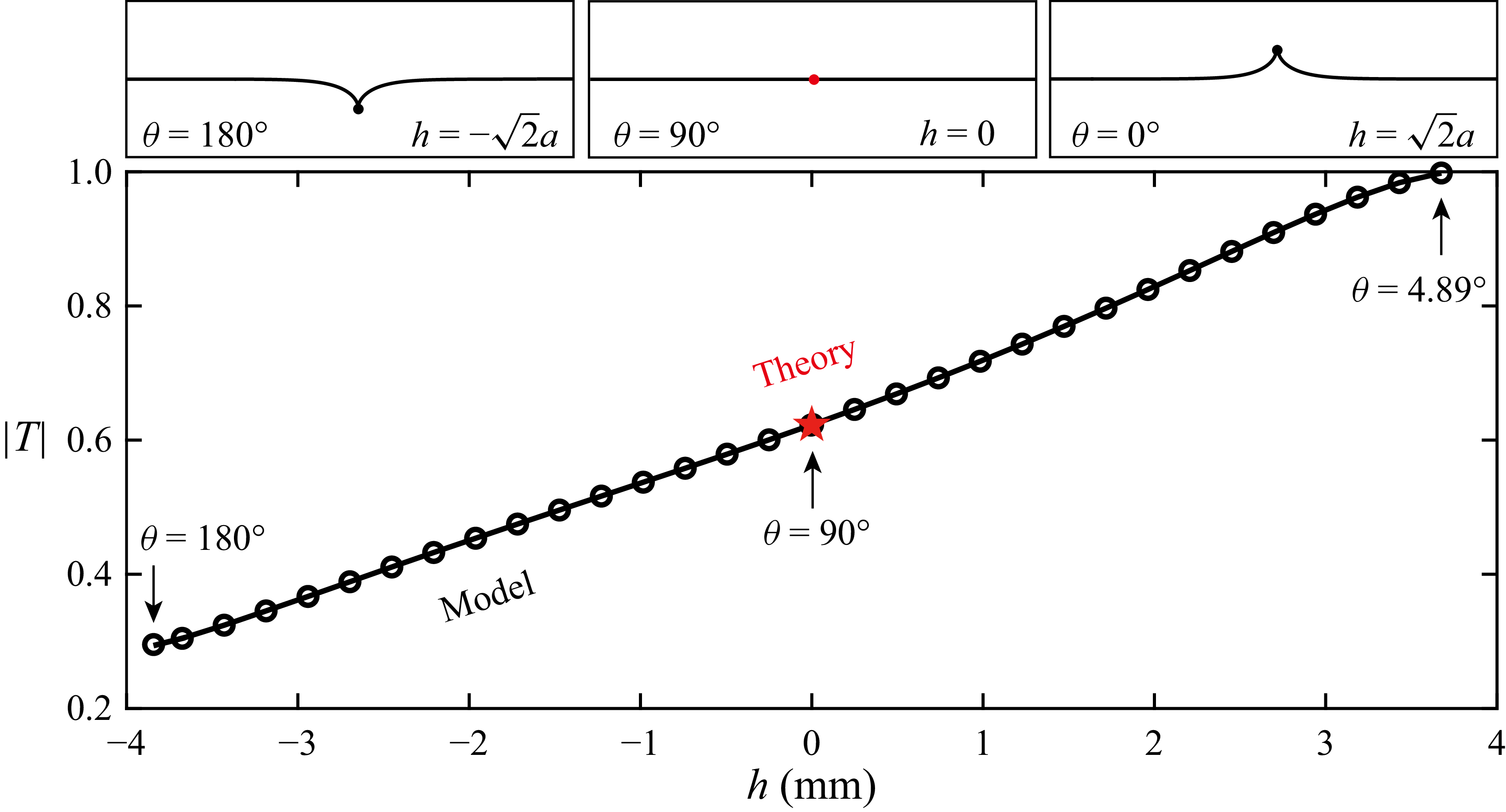


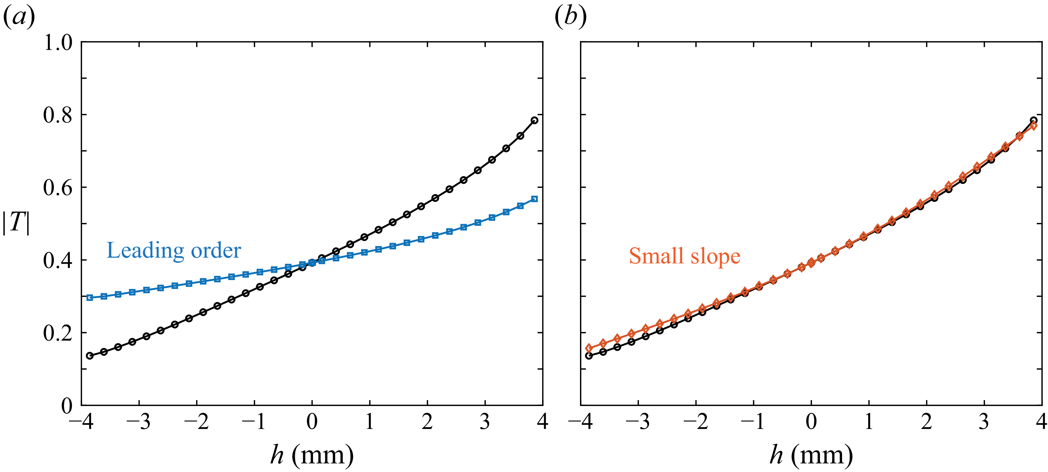


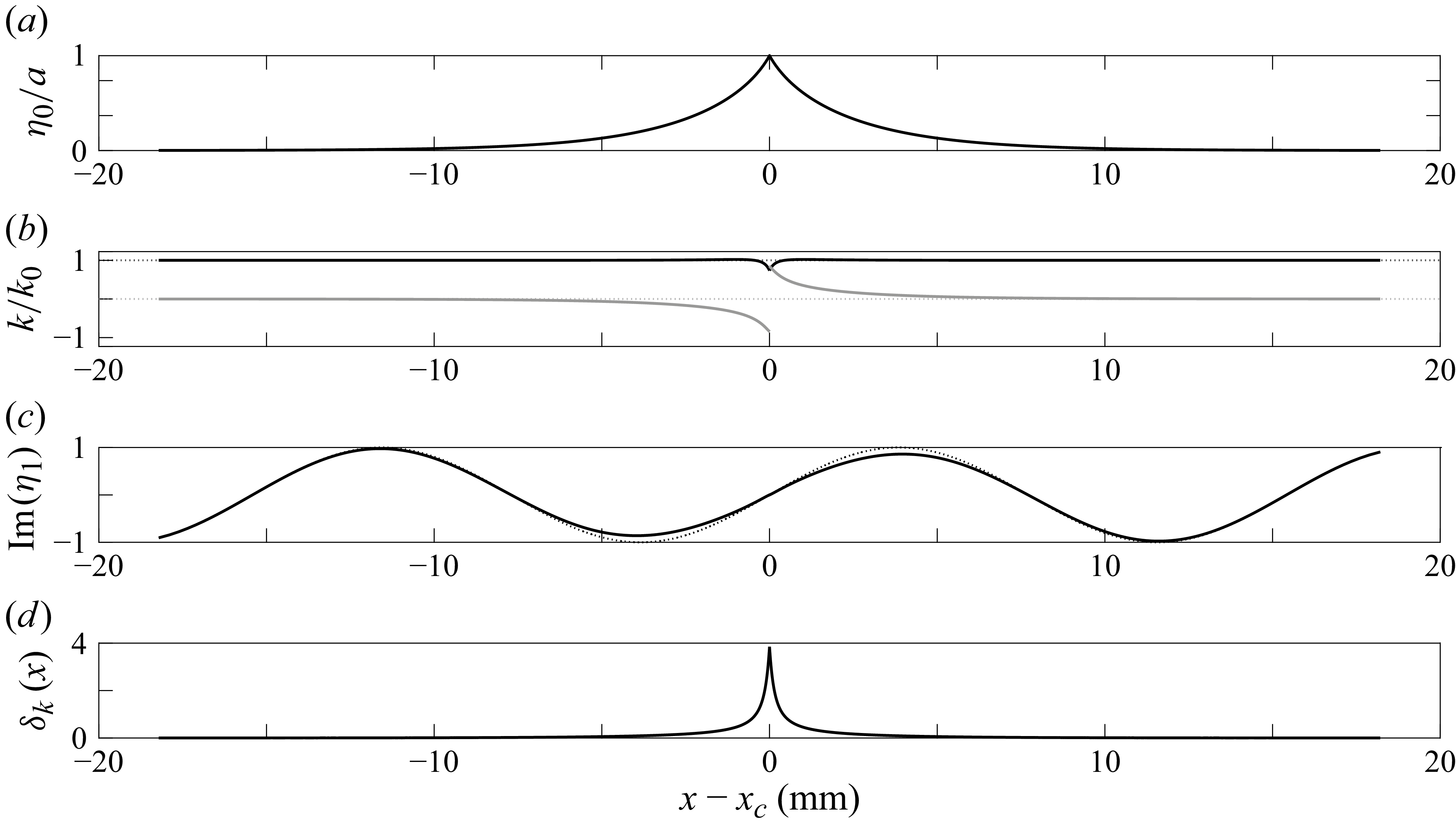


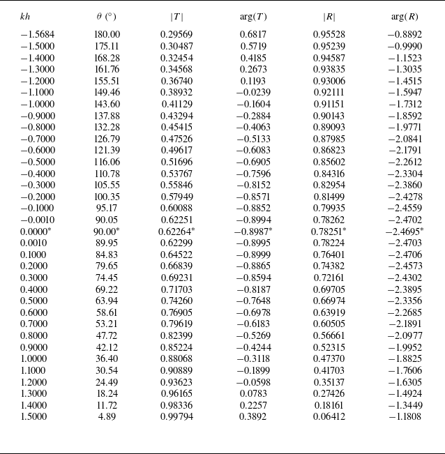


 Open access