


1. Introduction
Variations in seawater temperature and salinity levels establish ocean stratification. Baroclinic forcings within such stratified fluid systems – e.g. tidal flow over bottom topography or opposing background currents – evolve into internal waves propagating along pycnoclines. One class of internal waves – internal solitary waves (ISWs) – can maintain a localised, single-hump structure at the pycnocline over an extended distance through a balance between nonlinear steepening and linear dispersion (Helfrich & Melville Reference Helfrich and Melville2006; Cavaliere et al. Reference Cavaliere, la Forgia, Adduce, Alpers, Martorelli and Falcini2021). The occurrence of ISWs is well documented through both in situ thermistor array and synthetic aperture radar imagery. The ISWs have been observed on continental shelves, in straits and in marginal seas (Apel Reference Apel2002; Duda et al. Reference Duda, Lynch, Irish, Beardsley, Ramp, Chiu, Tang and Yang2004). As they propagate, ISWs transport energy as well as biological and chemical constituents. The interaction between ISWs, bathymetry and ambient shear triggers vertical mixing and plays a key role in biogeochemical processes. For example, mixing often introduces bottom nutrients into the upper water column, thereby fertilising the local region and modifying primary production and related biological processes.
Near-surface obstructions, such as naturally occurring macroalgae mats (e.g. the Sargasso Sea), macroalgae farms, engineered offshore platforms, and sea ice, have the potential to modify the propagation of ISWs. The existence of these obstructions may therefore alter the sustained propagation of ISWs as well as interfacial mixing processes.
Previous investigations into the interaction between ISWs and floating ice have characterised the influence of ice type, ice shape and submergence depth. The experimental study by Carr et al. (Reference Carr2019) explored interactions between ISWs and various ice types, including level, grease and nilas ice. Although not explicitly quantified, the effective porosity of the different ice types may have influenced the resulting dynamics. This study also demonstrated that while ice floes with a shallow submergence depth (relative to the upper-layer depth of the two-layer system) impose a negligible impact on ISWs, deeper submergence significantly alters the ISW evolution. Under conditions of deep submergence, small-amplitude ISWs can be completely dissipated by the obstruction, while large-amplitude ISWs can still propagate with the formation of Kelvin–Helmholtz billows beneath the ice. For the level ice case, the transport speed of long ice floes normalised by the wave speed was found to depend linearly on the length of the ice floe normalised by the wavelength. Subsequent numerical studies by Zhang et al. (Reference Zhang, Xu, Li, You, Yin, Robertson and Zheng2022) and Terletska, Maderich & Tobisch (Reference Terletska, Maderich and Tobisch2024) investigated the influence of fixed ice geometry on ISW propagation. Upon impact, the incident ISW typically disintegrates, radiating energy into smaller secondary waves. Specifically, Zhang et al. (Reference Zhang, Xu, Li, You, Yin, Robertson and Zheng2022) observed wave overturning and trailing edge steepening as the ISW exited the interaction with a deeper obstruction. Their results suggest that the effects of ice shape, width and roughness are secondary to the ice height, which dictates the blockage ratio. Different regimes of energy transformation emerge, depending on the blockage ratio. A solid obstruction thinner than the upper-layer depth of a two-layer system favours energy transmission with dissipation, whereas an obstruction thicker than the upper-layer depth promotes reflection over transmission. The interaction between ISWs and freely floating ice structures was examined by Hartharn-Evans, Carr & Stastna (Reference Hartharn-Evans, Carr and Stastna2024) using weighted floats. Under the freely floating condition, the ice motions are primarily governed by the ice length and the ISW amplitude. Floats with lengths significantly shorter than the ISW wavelength behave as a fluid particle with minimal flow disruption. In contrast, floats with lengths exceeding the ISW wavelength experience increased hydrodynamic resistance from the still water on either side of the ISW, resulting in a reduced translation velocity relative to the phase speed of the ISW.
While studies on the interactions between ISWs and floating solid obstructions have increased in the past five years, relatively less attention has been paid to the interaction between ISWs and surface porous objects, as will be presented herein. The porous canopy structure allows partial flow penetration. Canopy-scale vortices within the porous structure and the shear at the canopy interface are expected to augment dissipation. In addition to providing insight into the interaction between ISWs and surface structures, this study can inform offshore macroalgal farming, proposed as a sustainable strategy for greenhouse gas absorption, biofuel production and food supply (Frieder et al. Reference la Forgia, Cavaliere, Adduce and Falcini2022; Arzeno-Soltero et al. Reference Arzeno-Soltero, Saenz, Frieder, Long, DeAngelo, Davis and Davis2023). Understanding the fundamental dynamics of ISW–canopy interaction provides a foundation for predicting the impacts and benefits to coastal processes. Prior studies have provided substantial insight into the interaction between submerged canopies and unidirectional or wave-induced flows. For a unidirectional flow within an unstratified fluid, the velocity profile remains quasi-logarithmic for sparse submerged canopies. For a dense submerged canopy, the drag discontinuity at the canopy tip generates a shear layer, which can induce canopy-scale vortices that control the exchange within the canopy and overflow (Nepf Reference Nepf2012). For progressive wave forcing within an unstratified fluid, a mean current in the direction of wave propagation is generated within the submerged canopy by a non-zero wave stress (Luhar et al. Reference Luhar, Coutu, Infantes, Fox and Nepf2010). The mean current can promote the net horizontal transport of suspended sediment and organic matter within the canopy structure. In some ways, surface canopies may be regarded as the inverted analogue of submerged canopies with similar behaviours. However, the free-stream flow bounded by the bottom edge of the surface canopy and the solid bed confines the flow development. The no-slip bottom wall boundary imposes a stronger physical restriction on the growth of the shear layer, which is responsible for generating the coherent vortices at the bottom edge of the surface canopy (Plew Reference Plew2011). With the additional background stratification, structures resembling Kelvin–Helmholtz vortices emerge as the shear layer at the bottom edge of the canopy interacts with the underlying stratification, radiating small-scale internal waves (Bo, McWilliams & Chamecki Reference Bo, McWilliams and Chamecki2025). Sufficiently strong stratification is shown to suppress vertical mixing, favouring a horizontal motion instead, and thereby enhancing the dissipation within the canopy structure (Plew et al. Reference Plew, Spigel, Stevens, Nokes and Davidson2006).
In this paper, the effect of a surface canopy on ISWs is examined experimentally and numerically in a system of miscible two-layer stratification. This two-layer system creates stronger confinement between the bottom of the canopy and the pycnocline, which can lead to enhanced interactions between the shear layers generated by the ISWs at the bottom of the canopy and at the pycnocline. Through experimental and numerical efforts, we characterise the influence of canopy porosity and length on the propagation of ISWs of varying amplitudes. Section 2 describes the experimental configuration, measurement techniques and explored parameter maps. Section 3 describes the complementary numerical modelling effort, including the permeability specification for the canopy. Section 4 presents amplitude evolution during the interaction, the corresponding mechanisms at different interacting phases, and the associated energy transformation. Finally, concluding remarks are offered in § 5. An additional simulation-based discussion of extended canopy length in order to isolate transient effects is provided in Appendix A.
(a) Schematic for the experimental set-up of interactions between ISWs and surface porous canopies. (b) Photo image of the JAW.

2. Experimental method
2.1. Experimental set-up
The ISWs were generated by a jet-array wave maker (JAW) (Chu, Lynett & Luhar Reference Chu, Lynett and Luhar2025) in a $2.2$
m long,
$2.2$
m long, $0.2$
m wide, and
$0.2$
m wide, and $0.5$
m deep acrylic flume. Within the flume, a miscible two-layer system was set up as background stratification, separated by a thin pycnocline. The lower layer was filled with a salt solution of density
$0.5$
m deep acrylic flume. Within the flume, a miscible two-layer system was set up as background stratification, separated by a thin pycnocline. The lower layer was filled with a salt solution of density $\rho _2 = 1020 \pm 2$
kg m−3. This was confirmed via multiple measurements using a salinity probe. Fresh water with density
$\rho _2 = 1020 \pm 2$
kg m−3. This was confirmed via multiple measurements using a salinity probe. Fresh water with density $\rho _1 = 998$
kg m−3 was then introduced into the flume until the total depth
$\rho _1 = 998$
kg m−3 was then introduced into the flume until the total depth $H = h_1 + h_2$
reached approximately
$H = h_1 + h_2$
reached approximately $11$
cm. The experiments were carried out with fixed nominal depth ratio
$11$
cm. The experiments were carried out with fixed nominal depth ratio $h_2/h_1 = 9/2$
, with nominal wave amplitudes
$h_2/h_1 = 9/2$
, with nominal wave amplitudes $a = -1, -1.5, -2$
cm.
$a = -1, -1.5, -2$
cm.
The JAW system is composed of two independent, piston-driven cylinders, as shown in figure 1(b). The cylinders containing fresh water and salt solution are connected to the upper and lower layers of the flume, respectively. The pistons were driven by servo motors (Kollmorgen AKM44J), which were controlled using MATLAB scripts interfaced with a National Instruments data acquisition system (NI 6009) to generate prescribed volumetric fluxes (inflows and outflows) within each layer. To ensure near-uniform flow within each layer, fluid was driven from each cylinder through four uniformly spaced pipes, which subsequently fed through honeycomb flow straighteners. For each trial, the signal to drive the JAW system was prescribed based on the closed-form extended Korteweg–de Vries (eKdV) solution using the nominal layer depths and amplitude to determine the required mass flux for the inlet boundary conditions. While the fully nonlinear theories, such as the Dubreil–Jacotin–Long (DJL) equation, may provide a more mathematically rigorous description of ISWs (Lamb Reference Lamb2023), there are minimal differences in the computed inlet time series and initial wave profiles predicted using the DJL solver (Dunphy, Subich & Stastna Reference Dunphy, Subich and Stastna2011) and the eKdV solution for the parameter ranges considered here. We recognise that the wave evolves and transforms during the wave–structure interaction, such that the term ‘internal solitary wave’ may not apply. However, for simplicity, we retain the term ISW to describe the wave throughout the paper. The influence of a slight variation between nominal and actual layer depths on wave generation using the JAW system is addressed in Chu et al. (Reference Chu, Lynett and Luhar2025). For the conditions considered in this paper, the actual layer depths differed from the nominal values by ${\lt } 0.2$
cm. This is expected to translate into wave amplitude differences of 10 % or less relative to the nominal prescribed values.
${\lt } 0.2$
cm. This is expected to translate into wave amplitude differences of 10 % or less relative to the nominal prescribed values.
Surface canopy structures were installed approximately $100$
cm downstream of the inlet, positioned just beneath the free surface at vertical location
$100$
cm downstream of the inlet, positioned just beneath the free surface at vertical location $z_c = 10$
cm as shown in figure 1(a). The canopies were rigidly constrained and not allowed to drift with the waves. The canopies were three-dimensionally printed to span the full channel width, with constant height
$z_c = 10$
cm as shown in figure 1(a). The canopies were rigidly constrained and not allowed to drift with the waves. The canopies were three-dimensionally printed to span the full channel width, with constant height $h_c = 1$
cm. Each canopy consisted of uniform element width
$h_c = 1$
cm. Each canopy consisted of uniform element width $d$
, equal streamwise and lateral spacing
$d$
, equal streamwise and lateral spacing $s_x = s_y$
, and vertical spacing
$s_x = s_y$
, and vertical spacing $s_z$
, as illustrated in figure 2(a). Two canopy lengths (
$s_z$
, as illustrated in figure 2(a). Two canopy lengths ( $l_c = 5h_1 = 10$
cm and
$l_c = 5h_1 = 10$
cm and $l_c = 10h_1 = 20$
cm) and two porosity levels (
$l_c = 10h_1 = 20$
cm) and two porosity levels ( $n = 0.648, 0.964$
) were tested. For the range of ISWs generated in our experiments, the characteristic wavelengths remained at
$n = 0.648, 0.964$
) were tested. For the range of ISWs generated in our experiments, the characteristic wavelengths remained at $\lambda \approx 55$
cm. Consequently, both canopy lengths were significantly shorter than the wavelength (
$\lambda \approx 55$
cm. Consequently, both canopy lengths were significantly shorter than the wavelength ( $l_c \lt 0.5 \lambda$
). Thus transient edge effects from the surface canopy are expected during the interaction. To isolate these transient effects, a numerical study is presented in Appendix A using an extended canopy with canopy length
$l_c \lt 0.5 \lambda$
). Thus transient edge effects from the surface canopy are expected during the interaction. To isolate these transient effects, a numerical study is presented in Appendix A using an extended canopy with canopy length $l_c \gt 2 \lambda$
. The printed dimensions were
$l_c \gt 2 \lambda$
. The printed dimensions were $(d, s_x=s_y, s_z) = (0.4, 0.6, 0.6)$
cm for the lower-porosity canopies
$(d, s_x=s_y, s_z) = (0.4, 0.6, 0.6)$
cm for the lower-porosity canopies $(n=0.648)$
, and
$(n=0.648)$
, and $(d, s_x=s_y, s_z) = (0.2, 2.3, 0.8)$
cm for the higher-porosity canopies
$(d, s_x=s_y, s_z) = (0.2, 2.3, 0.8)$
cm for the higher-porosity canopies $(n=0.964)$
.
$(n=0.964)$
.
(a) Cross-sectional view and nomenclature of the canopy structure. (b) Isometric views of the transitional canopy with porosity $n=0.964$
. (c) Isometric views of the dense canopy with porosity
$n=0.964$
. (c) Isometric views of the dense canopy with porosity $n=0.648$
.
$n=0.648$
.

These two porosities were chosen to span the so-called dense and transitional regimes for canopy flows (Nepf Reference Nepf2012). Previous work shows that flow penetration into canopies from adjacent non-vegetated regions depends on the dimensionless frontal area ratio $\lambda_{\kern-1pt f}$
, which represents the frontal area of the canopy per unit of planar area in the streamwise direction. For
$\lambda_{\kern-1pt f}$
, which represents the frontal area of the canopy per unit of planar area in the streamwise direction. For $\lambda_{\kern-1pt f} \ll 0.1$
, the canopy can be considered sparse, and there is significant flow penetration into the canopy. For
$\lambda_{\kern-1pt f} \ll 0.1$
, the canopy can be considered sparse, and there is significant flow penetration into the canopy. For $\lambda_{\kern-1pt f} \gg 0.1$
, the canopy can be considered dense. In this ‘dense’ case, a region of strong shear develops at the interface between the canopy and the adjacent unobstructed flow. This canopy shear layer can generate large-scale turbulent rollers via mechanisms similar to the Kelvin–Helmholtz instability. Canopies with
$\lambda_{\kern-1pt f} \gg 0.1$
, the canopy can be considered dense. In this ‘dense’ case, a region of strong shear develops at the interface between the canopy and the adjacent unobstructed flow. This canopy shear layer can generate large-scale turbulent rollers via mechanisms similar to the Kelvin–Helmholtz instability. Canopies with $\lambda_{\kern-1pt f} \approx 0.1$
exhibit transitional behaviour between the sparse and dense regimes. For the canopy geometries considered in this paper, the less porous canopy has frontal area ratio
$\lambda_{\kern-1pt f} \approx 0.1$
exhibit transitional behaviour between the sparse and dense regimes. For the canopy geometries considered in this paper, the less porous canopy has frontal area ratio $\lambda_{\kern-1pt f} \approx 0.64$
, and the more porous canopy has frontal area ratio
$\lambda_{\kern-1pt f} \approx 0.64$
, and the more porous canopy has frontal area ratio $\lambda_{\kern-1pt f} \approx 0.16$
. These canopies may therefore be classified as dense and transitional, respectively.
$\lambda_{\kern-1pt f} \approx 0.16$
. These canopies may therefore be classified as dense and transitional, respectively.
Table 1 summarises the parameters for the $12$
experiments conducted. Each case is named after the prescribed wave amplitude (A), canopy length (L) and canopy type – dense (D) or transitional (T) – corresponding to its porosity. In this table,
$12$
experiments conducted. Each case is named after the prescribed wave amplitude (A), canopy length (L) and canopy type – dense (D) or transitional (T) – corresponding to its porosity. In this table, $h_{1,m}$
and
$h_{1,m}$
and $h_{2,m}$
are the measured layer depths obtained using planar laser-induced fluorescence (PLIF), as described below. For the following figures, experimental data are represented by hollow markers as listed in table 1, while the simulation results are represented by the corresponding solid markers.
$h_{2,m}$
are the measured layer depths obtained using planar laser-induced fluorescence (PLIF), as described below. For the following figures, experimental data are represented by hollow markers as listed in table 1, while the simulation results are represented by the corresponding solid markers.
Theoretical and measured values used for the experiments.

2.2. Measurement techniques
Interactions between ISWs and canopies were captured by synchronised PLIF and two-dimensional two-component particle imaging velocimetry (PIV). Polyamide particles with mean diameter $55\,{\unicode{x03BC}}$
m were introduced via floating sponges during the establishment of the upper layer for particle tracking. While the particles are slightly denser than both the fresh water (
$55\,{\unicode{x03BC}}$
m were introduced via floating sponges during the establishment of the upper layer for particle tracking. While the particles are slightly denser than both the fresh water ( $\rho _1 = 998$
kg m−3) and the salt solution (
$\rho _1 = 998$
kg m−3) and the salt solution ( $\rho _2 \approx 1020$
kg m−3), with mean density
$\rho _2 \approx 1020$
kg m−3), with mean density $1030$
kg m−3, the settling rate is negligible over the time scale of the ISW passage. Additional details are provided in Chu et al. (Reference Chu, Lynett and Luhar2025). However, PIV measurements in prior work were subject to insufficient particle density in the uppermost region of the freshwater layer, which is the location of our surface canopy structure, due to particle settling effects (Chu et al. Reference Chu, Lynett and Luhar2025). To ensure sufficient seeding density around the canopy, a revised two-step filling method was employed here. First, the freshwater layer was built with sponges floating on the free surface until the water level reached the canopy height. Second, the sponges were repositioned on top of the canopy as illustrated in figure 3, with the seeded fresh water slowly dripping into the upper layer. Due to the sponge repositioning, the pycnocline thickness estimated from PLIF increased to approximately
$1030$
kg m−3, the settling rate is negligible over the time scale of the ISW passage. Additional details are provided in Chu et al. (Reference Chu, Lynett and Luhar2025). However, PIV measurements in prior work were subject to insufficient particle density in the uppermost region of the freshwater layer, which is the location of our surface canopy structure, due to particle settling effects (Chu et al. Reference Chu, Lynett and Luhar2025). To ensure sufficient seeding density around the canopy, a revised two-step filling method was employed here. First, the freshwater layer was built with sponges floating on the free surface until the water level reached the canopy height. Second, the sponges were repositioned on top of the canopy as illustrated in figure 3, with the seeded fresh water slowly dripping into the upper layer. Due to the sponge repositioning, the pycnocline thickness estimated from PLIF increased to approximately $1.5$
cm in the experiments considered here (as opposed to remaining below
$1.5$
cm in the experiments considered here (as opposed to remaining below $1$
cm in the previous work). The methodology for characterising the pycnocline position (
$1$
cm in the previous work). The methodology for characterising the pycnocline position ( $\zeta$
) and thickness (
$\zeta$
) and thickness ( $\Delta \zeta$
) from the PLIF data follows the framework established by Chu et al. (Reference Chu, Lynett and Luhar2025), in which a hyperbolic tangent function is fitted to the PLIF intensity profile. The inflection point of the fitted profile defines the vertical position of the pycnocline, and the pycnocline thickness is determined by the coefficient parametrising the steepness of the hyperbolic tangent function; half the pycnocline thickness is absorbed into each layer depth (
$\Delta \zeta$
) from the PLIF data follows the framework established by Chu et al. (Reference Chu, Lynett and Luhar2025), in which a hyperbolic tangent function is fitted to the PLIF intensity profile. The inflection point of the fitted profile defines the vertical position of the pycnocline, and the pycnocline thickness is determined by the coefficient parametrising the steepness of the hyperbolic tangent function; half the pycnocline thickness is absorbed into each layer depth ( $h_{1,m}, h_{2,m}$
).
$h_{1,m}, h_{2,m}$
).
An illustration of the two-step filling method to ensure sufficient particle density in the upper layer.

(a) Schematic of the synchronised PLIF and PIV measurement system. Observation window coverage for (bi) short canopy, (bii) long canopy conditions.

The synchronised PLIF and PIV system consisted of two 8-bit CMOS monochrome cameras (Mako-U-130B) of $1024 \times 1280$
pixel resolution operating at
$1024 \times 1280$
pixel resolution operating at $50$
Hz for
$50$
Hz for $40$
s. The measurement duration was chosen to ensure that the entirety of the ISW was captured. A 5 W continuous laser with emission wavelength 532 nm and built-in sheet generation optics was used to illuminate the flow field from below (figure 4
a). For the PLIF measurements, Rhodamine 6G dye with peak excitation wavelength 525 nm and peak emission wavelength 548 nm was pre-mixed with the fresh water. An optical filter with a passband between 536 nm to 564 nm was therefore used to isolate the fluorescent freshwater layer. Assuming single-pixel resolution for the PLIF measurements, the dye field is resolved to better than 0.2 mm.
$40$
s. The measurement duration was chosen to ensure that the entirety of the ISW was captured. A 5 W continuous laser with emission wavelength 532 nm and built-in sheet generation optics was used to illuminate the flow field from below (figure 4
a). For the PLIF measurements, Rhodamine 6G dye with peak excitation wavelength 525 nm and peak emission wavelength 548 nm was pre-mixed with the fresh water. An optical filter with a passband between 536 nm to 564 nm was therefore used to isolate the fluorescent freshwater layer. Assuming single-pixel resolution for the PLIF measurements, the dye field is resolved to better than 0.2 mm.
The cameras shared an overlapping field of view measuring $12\times15\ \text{cm}^2$
. For the short canopy case
$12\times15\ \text{cm}^2$
. For the short canopy case $(l_c/h_1 = 5)$
, the field of view extended from upstream to downstream of the canopy, enabling full observation of the interaction process, as illustrated in figure 4(bi). However, for the long canopy case
$(l_c/h_1 = 5)$
, the field of view extended from upstream to downstream of the canopy, enabling full observation of the interaction process, as illustrated in figure 4(bi). However, for the long canopy case $(l_c/h_1 = 10)$
, the field of view could not cover the entire canopy length. As such, the field of view was positioned to focus on the downstream half of the canopy. Specifically, the field of view encompassed slightly more than the downstream half of the canopy with an additional
$(l_c/h_1 = 10)$
, the field of view could not cover the entire canopy length. As such, the field of view was positioned to focus on the downstream half of the canopy. Specifically, the field of view encompassed slightly more than the downstream half of the canopy with an additional $2$
cm beyond, as illustrated in figure 4(bii). The MATLAB PIVLab package was used to post-process the images using a multi-pass algorithm. The initial pass involved a
$2$
cm beyond, as illustrated in figure 4(bii). The MATLAB PIVLab package was used to post-process the images using a multi-pass algorithm. The initial pass involved a $64\times64\ \text{pixel}^2$
interrogation window. Two subsequent passes with
$64\times64\ \text{pixel}^2$
interrogation window. Two subsequent passes with $32\times32\ \text{pixel}^2$
interrogation windows with
$32\times32\ \text{pixel}^2$
interrogation windows with $50$
% overlap yielded
$50$
% overlap yielded $52\times32$
velocity vectors per snapshot.
$52\times32$
velocity vectors per snapshot.
3. Numerical model
3.1. Model set-up
Numerical simulations of ISW interactions with surface canopies were conducted using ANSYS Fluent. A two-dimensional computational domain was designed to match the experimental set-up illustrated in the previous section, consisting of total depth $H = 0.11$
m and flume length
$H = 0.11$
m and flume length $L=2.2$
m. The domain was discretised using a uniform hexahedral mesh with resolution
$L=2.2$
m. The domain was discretised using a uniform hexahedral mesh with resolution $\Delta x = 2\times 10^{-3}$
m and
$\Delta x = 2\times 10^{-3}$
m and $\Delta z = 1\times 10^{-3}$
m. Grid resolution in the vertical direction
$\Delta z = 1\times 10^{-3}$
m. Grid resolution in the vertical direction $(z)$
was selected to be no greater than 10 % of the smallest wave amplitude. Grid resolution in the streamwise
$(z)$
was selected to be no greater than 10 % of the smallest wave amplitude. Grid resolution in the streamwise $(x)$
direction was controlled by the grid aspect ratio (
$(x)$
direction was controlled by the grid aspect ratio ( $\Delta x / \Delta z$
) to avoid amplified numerical dissipation. To replicate the experimental conditions, the initial stratification was imposed using a hyperbolic tangent density profile with fixed pycnocline thickness 1.5 cm. The upper freshwater layer was assigned density
$\Delta x / \Delta z$
) to avoid amplified numerical dissipation. To replicate the experimental conditions, the initial stratification was imposed using a hyperbolic tangent density profile with fixed pycnocline thickness 1.5 cm. The upper freshwater layer was assigned density $\rho _1 = 998$
kg m−3 and dynamic viscosity
$\rho _1 = 998$
kg m−3 and dynamic viscosity $\mu _1 = 1.00 \times 10^{-3}$
Pa s, while the lower salt solution layer was defined by
$\mu _1 = 1.00 \times 10^{-3}$
Pa s, while the lower salt solution layer was defined by $\rho _2 = 1020$
kg m−3 and dynamic viscosity
$\rho _2 = 1020$
kg m−3 and dynamic viscosity $\mu _2 = 1.09 \times 10^{-3}$
Pa s.
$\mu _2 = 1.09 \times 10^{-3}$
Pa s.
To reproduce the wave-generation mechanism of the JAW system, mass flow inlets were applied at the upstream boundary of both layers, as illustrated in figure 5(a). The upper channel allowed only fresh water ( $\dot {m_1}$
), while the lower channel allowed only ocean water (
$\dot {m_1}$
), while the lower channel allowed only ocean water ( $\dot {m_2}$
). The mass flow rates were calculated by integrating the horizontal velocity profiles from the eKdV solution across the respective layer thicknesses, multiplied by the corresponding fluid density. No-slip boundary conditions were imposed along the channel walls and flume bed. The top surface was modelled as a no-shear boundary to approximate the free surface.
$\dot {m_2}$
). The mass flow rates were calculated by integrating the horizontal velocity profiles from the eKdV solution across the respective layer thicknesses, multiplied by the corresponding fluid density. No-slip boundary conditions were imposed along the channel walls and flume bed. The top surface was modelled as a no-shear boundary to approximate the free surface.
A mixture model was employed to simulate the multiphase configuration of the two-layer stratified system. Turbulence was modelled using the realisable $k\text{-}\epsilon$
Reynolds-averaged Navier–Stokes model. While the
$k\text{-}\epsilon$
Reynolds-averaged Navier–Stokes model. While the $k\text{-}\epsilon$
model has known limitations in handling strong adverse pressure gradients, recent comparisons with field measurements (Trowbridge et al. Reference Trowbridge, Helfrich, Reeder, Medley, Chang, Jan, Ramp and Yang2025) demonstrate its predictive accuracy in the bottom boundary layer beneath ISWs during free-stream acceleration and early deceleration. However, the model is unable to reproduce observations during the late deceleration and within the wake. In the present two-dimensional study, the
$k\text{-}\epsilon$
model has known limitations in handling strong adverse pressure gradients, recent comparisons with field measurements (Trowbridge et al. Reference Trowbridge, Helfrich, Reeder, Medley, Chang, Jan, Ramp and Yang2025) demonstrate its predictive accuracy in the bottom boundary layer beneath ISWs during free-stream acceleration and early deceleration. However, the model is unable to reproduce observations during the late deceleration and within the wake. In the present two-dimensional study, the $k\text{-}\epsilon$
model is employed primarily to characterise the macroscopic ISW–canopy interaction. The realisable formulation was specifically selected for its improved performance in capturing flow separation and boundary layers with variable eddy viscosity. To ensure accurate reproduction of wave amplitude evolution, the model coefficients within the
$k\text{-}\epsilon$
model is employed primarily to characterise the macroscopic ISW–canopy interaction. The realisable formulation was specifically selected for its improved performance in capturing flow separation and boundary layers with variable eddy viscosity. To ensure accurate reproduction of wave amplitude evolution, the model coefficients within the $k\text{-}\epsilon$
formulation were calibrated to avoid overprediction of numerical dissipation relative to experimental measurements. Specifically, the coefficients were set as
$k\text{-}\epsilon$
formulation were calibrated to avoid overprediction of numerical dissipation relative to experimental measurements. Specifically, the coefficients were set as $c_{2,\epsilon } = 1.6$
,
$c_{2,\epsilon } = 1.6$
, $\sigma _k =0.8$
and
$\sigma _k =0.8$
and $\sigma _\epsilon =0.9$
. Numerical solution procedures employed the coupled pressure–velocity scheme combined with the PRESTO pressure discretisation. Second-order implicit upwind schemes were applied to all transport equations, including momentum, turbulent kinetic energy, dissipation rate and transient formulation. A fixed time step
$\sigma _\epsilon =0.9$
. Numerical solution procedures employed the coupled pressure–velocity scheme combined with the PRESTO pressure discretisation. Second-order implicit upwind schemes were applied to all transport equations, including momentum, turbulent kinetic energy, dissipation rate and transient formulation. A fixed time step $ \Delta t = 5 \times 10^{-3}$
s was employed throughout all simulations. This value was selected to satisfy the Courant–Friedrichs–Lewy (CFL) stability criteria. The CFL number was estimated based on the dominant streamwise propagation of an ISW of
$ \Delta t = 5 \times 10^{-3}$
s was employed throughout all simulations. This value was selected to satisfy the Courant–Friedrichs–Lewy (CFL) stability criteria. The CFL number was estimated based on the dominant streamwise propagation of an ISW of $a = 2$
cm by using the nominal phase speed
$a = 2$
cm by using the nominal phase speed $c$
as the upper limit for the horizontal particle speed. This estimation resulted in a maximum CFL number
$c$
as the upper limit for the horizontal particle speed. This estimation resulted in a maximum CFL number $c\, \Delta t/ \Delta x \approx 0.18$
.
$c\, \Delta t/ \Delta x \approx 0.18$
.
Figure 5(b) presents a snapshot of density, horizontal velocity and vertical velocity contours of a simulated ISW corresponding to $(h_1, h_2, a) = (2,9,2)$
cm, evaluated
$(h_1, h_2, a) = (2,9,2)$
cm, evaluated $1$
m downstream from the inlet. For consistency in the subsequent analysis, the streamwise coordinate origin
$1$
m downstream from the inlet. For consistency in the subsequent analysis, the streamwise coordinate origin $(x=0)$
is defined at
$(x=0)$
is defined at $1$
m downstream from the inlet, where the leading edge of the surface canopies would otherwise be. The wave profile of the generated ISW in our numerical model is closely aligned with the eKdV solution for the same layer depths and wave amplitude.
$1$
m downstream from the inlet, where the leading edge of the surface canopies would otherwise be. The wave profile of the generated ISW in our numerical model is closely aligned with the eKdV solution for the same layer depths and wave amplitude.
(a) Schematic showing the numerical model. (b) Density contour for a simulated ISW. The black dashed curve represents the analytical eKdV profile used as the inlet boundary condition.

3.2. Canopy zone characterisation
The surface canopy structure was modelled as a homogeneous porous zone within the computational domain, as illustrated in figure 5. The porous region was defined by a specified porosity $n$
, and a viscous resistance parameter
$n$
, and a viscous resistance parameter $1/K$
, representing the inverse of permeability (
$1/K$
, representing the inverse of permeability ( $K$
). While the porosity was directly calculated as listed in table 1, accurate determination of viscous resistance was more challenging in experiments due to the small measurable pressure gradient across our canopy dimensions.
$K$
). While the porosity was directly calculated as listed in table 1, accurate determination of viscous resistance was more challenging in experiments due to the small measurable pressure gradient across our canopy dimensions.
Previous experimental studies by Vijay & Luhar (Reference Vijay and Luhar2024) characterised discrete viscous resistance values for both isotropic and anisotropic porous substrates with cubic lattice geometries similar to those considered in this paper. However, no general predictive relationship was established for estimating the viscous resistance of these porous structures. In the present study, the following Kozeny–Carman (KC) equation was adopted as a base model for estimating permeability (Carman Reference Carman1939):
 \begin{align} K_{\textit{KC}} = \frac {\beta }{\sigma ^2} \frac {n^3}{(1-n)^2}. \end{align}
In this model, $\sigma$
represents the specific surface area for the structure, and
$\sigma$
represents the specific surface area for the structure, and $\beta$
is the so-called Kozeny constant, which depends on the specific porous geometry. The KC model was initially derived under the assumption of non-interconnected, parallel tube bundles as a simplified representation of complicated porous formations. More recent findings by Schulz et al. (Reference Schulz, Ray, Zech, Rupp and Knabner2019) indicate that a value
$\beta$
is the so-called Kozeny constant, which depends on the specific porous geometry. The KC model was initially derived under the assumption of non-interconnected, parallel tube bundles as a simplified representation of complicated porous formations. More recent findings by Schulz et al. (Reference Schulz, Ray, Zech, Rupp and Knabner2019) indicate that a value $\beta =0.2$
yields the best agreement with experimental data for irregular porous structures. The specific surface is defined as the surface area
$\beta =0.2$
yields the best agreement with experimental data for irregular porous structures. The specific surface is defined as the surface area $S_c$
divided by the solid volume
$S_c$
divided by the solid volume $V_c$
of a unit canopy cell. For the geometries considered in this paper, the unit canopy cell consists of a central cube with side length
$V_c$
of a unit canopy cell. For the geometries considered in this paper, the unit canopy cell consists of a central cube with side length $d$
, and three square columns oriented along the principal axes as shown in figure 6. As such, the specific surface area can be estimated using the equation
$d$
, and three square columns oriented along the principal axes as shown in figure 6. As such, the specific surface area can be estimated using the equation
 \begin{align} \sigma = \frac {S_c}{V_c} = \frac {6d^2 + 4 s_x d + 4 s_y d + 4 s_z d}{d^3 + d^2s_x + d^2 s_y + d^2 s_z}. \end{align}
Unit cell for the calculation of a specific surface.

To evaluate the applicability of the KC model for the cubic lattice geometries considered in this paper, the predicted resistance values were compared against the measurements reported by Vijay & Luhar (Reference Vijay and Luhar2024), as shown in table 2. The experiments of Vijay & Luhar (Reference Vijay and Luhar2024) considered cubic cell geometries with fixed stem thickness $d= 4\times 10^{-3}$
m and varying spacings in the principal directions. Each specimen was labelled with a three-letter code representing the spacings along the principal directions. Here, we consider the isotropic cases HHH, MMM and LLL, denoting high, medium and low spacings (i.e. going from more porous to less porous). As shown in table 2, the KC model provides a reasonable estimate of the measured viscous resistances, with predictions agreeing with the measurements within
$d= 4\times 10^{-3}$
m and varying spacings in the principal directions. Each specimen was labelled with a three-letter code representing the spacings along the principal directions. Here, we consider the isotropic cases HHH, MMM and LLL, denoting high, medium and low spacings (i.e. going from more porous to less porous). As shown in table 2, the KC model provides a reasonable estimate of the measured viscous resistances, with predictions agreeing with the measurements within $\pm 15\,\%$
for the HHH and MMM cases. For the densest LLL case considered by Vijay & Luhar (Reference Vijay and Luhar2024), the predicted viscous resistance is a factor of 2–3 times higher. Following this limited validation exercise, additional numerical sensitivity analyses were carried out to identify the most appropriate resistance values for the canopies considered in the experiments.
$\pm 15\,\%$
for the HHH and MMM cases. For the densest LLL case considered by Vijay & Luhar (Reference Vijay and Luhar2024), the predicted viscous resistance is a factor of 2–3 times higher. Following this limited validation exercise, additional numerical sensitivity analyses were carried out to identify the most appropriate resistance values for the canopies considered in the experiments.
Viscous resistance (permeability) estimates obtained using the KC model, and comparison with measurements by Vijay & Luhar (Reference Vijay and Luhar2024) for similar geometries.

Sensitivity tests evaluating the impact of the chosen viscous resistance on the integrated velocity error $e$
from (3.3).
$e$
from (3.3).

As a sensitivity test, numerical simulations were performed for the dense and transitional surface canopies subjected to ISWs using the exact viscous resistance values predicted by the KC model, and values multiplied by a factor of 5 lower and higher, i.e. corresponding to viscous resistances $5/K_{\textit{KC}}$
,
$5/K_{\textit{KC}}$
, $1/K_{\textit{KC}}$
and
$1/K_{\textit{KC}}$
and $1/5K_{\textit{KC}}$
. These tests compared the predicted and measured horizontal velocity profiles at the primary wave crest for ISWs of
$1/5K_{\textit{KC}}$
. These tests compared the predicted and measured horizontal velocity profiles at the primary wave crest for ISWs of $a = 2$
cm under the long transitional and long dense canopies (A2L2T and A2L2D). Velocity profiles were compared at the streamwise location
$a = 2$
cm under the long transitional and long dense canopies (A2L2T and A2L2D). Velocity profiles were compared at the streamwise location $x/h_1 = 10.5$
immediately downstream of the canopy, where experimental measurements were first available across the full water depth following the interaction between the ISW and the surface canopy. The difference was quantified using the
$x/h_1 = 10.5$
immediately downstream of the canopy, where experimental measurements were first available across the full water depth following the interaction between the ISW and the surface canopy. The difference was quantified using the $l_1$
norm, normalised by the nominal phase speed of the ISW,
$l_1$
norm, normalised by the nominal phase speed of the ISW, $c$
, defined as
$c$
, defined as
 \begin{align} e = \frac {1}{N} \sum _{i=1}^N\left |\frac {u_{n, i}-u_{m, i}}{c}\right |, \end{align}
where $u_n$
and
$u_n$
and $u_m$
are the numerical and measured horizontal velocity components, and
$u_m$
are the numerical and measured horizontal velocity components, and $N$
is the total number of data points across the entire water depth.
$N$
is the total number of data points across the entire water depth.
Comparison of horizontal velocity profiles between experiments and simulations with varying viscous resistances for cases (a) A2L2T and (b) A2L2D. Red hollow markers represent experimental profiles extracted from PIV measurements. Solid curves indicate $1/K_{\textit{KC}}$
, dashed curves indicate
$1/K_{\textit{KC}}$
, dashed curves indicate $5/K_{\textit{KC}}$
, and dotted curves indicate
$5/K_{\textit{KC}}$
, and dotted curves indicate $1/5K_{\textit{KC}}$
.
$1/5K_{\textit{KC}}$
.

Viscous resistance values scaled by a factor of $5$
from the KC model yielded better agreement with experimental results (table 3). For both the transitional and dense canopies, this adjustment more accurately captured the acceleration within the upper-layer fluid and the deceleration downstream of the canopy structure, as demonstrated by the velocity profiles in figure 7. Two factors may contribute to the consistently higher viscous resistance from the KC model. First, the unit cell used to compute the specific surface area (figure 6) neglects the contribution from the bottom stem surfaces. This exclusion may have a negligible impact on multi-layer canopy structures such as those used in the experiments by Vijay & Luhar (Reference Vijay and Luhar2024). However, it becomes increasingly significant in single-layer structures such as the canopies employed in the present study. In particular, the fully exposed lower interface of the canopy to the surrounding fluid likely enhances the impact of the bottom layer on overall resistance. Second, the KC model strictly applies only for the Darcy (creeping) flow regime, characterised by a low pore-scale Reynolds number
$5$
from the KC model yielded better agreement with experimental results (table 3). For both the transitional and dense canopies, this adjustment more accurately captured the acceleration within the upper-layer fluid and the deceleration downstream of the canopy structure, as demonstrated by the velocity profiles in figure 7. Two factors may contribute to the consistently higher viscous resistance from the KC model. First, the unit cell used to compute the specific surface area (figure 6) neglects the contribution from the bottom stem surfaces. This exclusion may have a negligible impact on multi-layer canopy structures such as those used in the experiments by Vijay & Luhar (Reference Vijay and Luhar2024). However, it becomes increasingly significant in single-layer structures such as the canopies employed in the present study. In particular, the fully exposed lower interface of the canopy to the surrounding fluid likely enhances the impact of the bottom layer on overall resistance. Second, the KC model strictly applies only for the Darcy (creeping) flow regime, characterised by a low pore-scale Reynolds number $Re_p \lt 1$
. In the present study, an estimated pore-scale Reynolds number
$Re_p \lt 1$
. In the present study, an estimated pore-scale Reynolds number $Re_p = u d/ \nu \gt O(10)$
– using the stem width
$Re_p = u d/ \nu \gt O(10)$
– using the stem width $d$
, the horizontal velocity component within the upper layer fluid
$d$
, the horizontal velocity component within the upper layer fluid $u$
, and the kinematic viscosity of water
$u$
, and the kinematic viscosity of water $\nu =10^{-6}$
m
$\nu =10^{-6}$
m $^2$
s−1 – places the flow in the transitional regime. The elevated
$^2$
s−1 – places the flow in the transitional regime. The elevated $Re_p$
implies enhanced inertial effects and stronger resistance compared to the conditions assumed in the original KC formulation. Despite these limitations, the numerical simulations capture experimental trends reasonably well using viscous resistance values of
$Re_p$
implies enhanced inertial effects and stronger resistance compared to the conditions assumed in the original KC formulation. Despite these limitations, the numerical simulations capture experimental trends reasonably well using viscous resistance values of $5/K_{\textit{KC}}$
.
$5/K_{\textit{KC}}$
.
4. Results
4.1. Wave amplitude evolution
Figure 8 presents the spatial evolution of ISW amplitudes under various canopy configurations. The pycnocline location $\zeta (t)$
is extracted from the PLIF visualisation using the method outlined in § 3.3 of Chu et al. (Reference Chu, Lynett and Luhar2025), whereby a hyperbolic tangent profile is fitted to the observed vertical fluorescence intensity. The error bars represent the measured pycnocline thickness. In the following discussion, wave amplitude
$\zeta (t)$
is extracted from the PLIF visualisation using the method outlined in § 3.3 of Chu et al. (Reference Chu, Lynett and Luhar2025), whereby a hyperbolic tangent profile is fitted to the observed vertical fluorescence intensity. The error bars represent the measured pycnocline thickness. In the following discussion, wave amplitude $a$
is defined as the maximum vertical displacement of the pycnocline from its initial undisturbed position within the primary wave crest. The corresponding streamwise position
$a$
is defined as the maximum vertical displacement of the pycnocline from its initial undisturbed position within the primary wave crest. The corresponding streamwise position $x$
denotes the location at which this maximum displacement is extracted, ensuring that the definition remains even when the wave profile departs from theoretical eKdV symmetry due to canopy interaction. In the numerical simulations, the pycnocline position is identified by locating the inflection point of the hyperbolic tangent density profile. To improve spatial precision beyond the grid resolution, the raw simulation data are interpolated to a refined vertical resolution
$x$
denotes the location at which this maximum displacement is extracted, ensuring that the definition remains even when the wave profile departs from theoretical eKdV symmetry due to canopy interaction. In the numerical simulations, the pycnocline position is identified by locating the inflection point of the hyperbolic tangent density profile. To improve spatial precision beyond the grid resolution, the raw simulation data are interpolated to a refined vertical resolution ${\rm d}z = 1 \times 10^{-3}$
m prior to extracting the pycnocline profile.
${\rm d}z = 1 \times 10^{-3}$
m prior to extracting the pycnocline profile.
Amplitude evolution in space for cases (a) no canopy, (b) short transitional canopy (L1T), (c) short dense canopy (L1D), (d) long transitional (L2T), (e) long dense canopy (L2D). Black, blue and red markers correspond to ISW amplitudes $a = 1, 1.5 ,2$
cm, respectively.
$a = 1, 1.5 ,2$
cm, respectively.

In the absence of a surface canopy (figure 8
a), wave amplitudes remain nearly constant throughout the entire observation window, with a total reduction of less than $1\,\%$
, in both experiments and simulations. Over a propagation distance
$1\,\%$
, in both experiments and simulations. Over a propagation distance $30h_1$
, the cumulative amplitude decay remains within
$30h_1$
, the cumulative amplitude decay remains within $2{-}3\,\%$
in the simulations. For the transitional canopy cases (figures 8
b,d), the wave amplitudes show dissipation of approximately 5–10 %, depending on the canopy length. There is a modest increase in wave amplitude at the leading edge of the canopy.
$2{-}3\,\%$
in the simulations. For the transitional canopy cases (figures 8
b,d), the wave amplitudes show dissipation of approximately 5–10 %, depending on the canopy length. There is a modest increase in wave amplitude at the leading edge of the canopy.
For the dense canopy cases (figures 8
c,e), pronounced nonlinear interactions are observed. Numerical simulations reveal an initial increase in wave amplitude upstream of the canopy, beginning at $x/h_1\approx -5$
. This amplitude growth, occurring prior to the wave crest reaching the canopy, is caused by the reflection imposed by the dense structure on the leading edge of the wave. The PLIF measurements effectively capture the final portion of this amplification (figure 8
c). The amplitude growth is followed by a sharp decay at
$x/h_1\approx -5$
. This amplitude growth, occurring prior to the wave crest reaching the canopy, is caused by the reflection imposed by the dense structure on the leading edge of the wave. The PLIF measurements effectively capture the final portion of this amplification (figure 8
c). The amplitude growth is followed by a sharp decay at $x/h_1\approx 0$
. This decay is observed in both numerical simulations and experimental measurements for the short dense canopy. Afterwards, a complex wave transformation process occurs over
$x/h_1\approx 0$
. This decay is observed in both numerical simulations and experimental measurements for the short dense canopy. Afterwards, a complex wave transformation process occurs over $0\lt x/h_1\lt 5$
. In the second half of the long dense canopy (
$0\lt x/h_1\lt 5$
. In the second half of the long dense canopy ( $5\lt x/h_1\lt 8$
), the wave amplitudes show a mild recovery and plateau. Downstream of the dense canopy, both the experiments and simulations show evidence of amplitude enhancement. The experimental PLIF measurements do not extend significantly beyond the canopies. However, the numerical simulations predict that this amplitude enhancement is sustained over a distance
$5\lt x/h_1\lt 8$
), the wave amplitudes show a mild recovery and plateau. Downstream of the dense canopy, both the experiments and simulations show evidence of amplitude enhancement. The experimental PLIF measurements do not extend significantly beyond the canopies. However, the numerical simulations predict that this amplitude enhancement is sustained over a distance $\approx 5h_1$
beyond the canopy. These complex transition processes at the leading and trailing edges of the dense canopies are described in greater detail in the following subsections.
$\approx 5h_1$
beyond the canopy. These complex transition processes at the leading and trailing edges of the dense canopies are described in greater detail in the following subsections.
Experimental results for the surface canopies, where available, generally show good agreement with the numerical predictions. Moreover, ISW amplitude does not appear to play a major role in dictating wave evolution underneath the canopies; the normalised amplitude profiles show reasonable collapse across all cases. Downstream of the canopy, however, the numerical simulations do show stronger wave amplitude dependence.
The trends observed in figure 8 indicate that the canopy density can play a significant role in shaping wave transformation. Although the present study considers only two canopy porosities, the results indicate that the geometric thresholds identified in prior work to delineate sparse and dense canopy behaviour (i.e. a strong shear layer only develops at the interface for $\lambda_{\kern-1pt f} \gg 0.1$
) remain appropriate for surface canopy –ISW interactions.
$\lambda_{\kern-1pt f} \gg 0.1$
) remain appropriate for surface canopy –ISW interactions.
4.2. Leading edge shoaling
As the ISW encounters the front edge of the dense canopy, the upper-layer flow is obstructed and diverted below the structure. This obstruction leads to a localised amplitude growth starting from $x/h_1 \approx -5$
, as shown in figures 8(c,e). Meanwhile, a positive vorticity packet begins to develop at the bottom edge of the canopy, as observed in figure 9(bi,bii). This vorticity growth is driven by enhanced shear at the canopy interface, induced by the diversion of high-momentum upper-layer fluid underneath the canopy as the ISW crest approaches. This shear and the intrinsic shear generated at the ISW pycnocline give rise to a counter-rotating vortex pair. The resulting vortex-induced jet accelerates the leading side of the ISW, as illustrated in figure 9(aii,bii). This process accounts for the rapid amplitude drop at
$x/h_1 \approx -5$
, as shown in figures 8(c,e). Meanwhile, a positive vorticity packet begins to develop at the bottom edge of the canopy, as observed in figure 9(bi,bii). This vorticity growth is driven by enhanced shear at the canopy interface, induced by the diversion of high-momentum upper-layer fluid underneath the canopy as the ISW crest approaches. This shear and the intrinsic shear generated at the ISW pycnocline give rise to a counter-rotating vortex pair. The resulting vortex-induced jet accelerates the leading side of the ISW, as illustrated in figure 9(aii,bii). This process accounts for the rapid amplitude drop at $x/h_1 \approx 0$
observed in the dense canopy cases in figures 8(c) and 8(e).
$x/h_1 \approx 0$
observed in the dense canopy cases in figures 8(c) and 8(e).
Simulation results for case A2L2D illustrate the leading edge shoaling process. (ai,aii) Consecutive normalised horizontal velocity contours in time. (bi,bii) Consecutive normalised vorticity contours in time. The solid black lines denote the pycnocline and surface canopy.

In contrast, for the transitional canopy cases, the upper-layer fluid is able to penetrate the canopy structure more easily. This yields a milder horizontal velocity deficit and reduced shear. As a result, the amplitude growth caused by flow obstruction as well as the subsequent amplitude reduction induced by the vortex-driven jet is much less pronounced. This trend is reflected in figures 8(b) and 8(d), where the wave amplitude remains relatively stable.
4.3. Wave crest adjustment
As the ISW propagates further into the canopy, the vortex-induced jet mechanism described in § 4.2 continues to shift upper-layer fluid volume from the trailing edge of the wave towards its leading edge. The wave crest adjustment process occurs over $0 \lt x/h_1 \lt 5$
, as shown in figures 8(c) and 8(e).
$0 \lt x/h_1 \lt 5$
, as shown in figures 8(c) and 8(e).
The forward adjustment of the primary wave crest is directly captured in the PLIF visualisation of the A2L1D configuration (figure 11). At an earlier time step, the primary wave crest remains positioned near the trailing edge of the ISW as indicated by the yellow arrow in figure 11(a), which is consistent with the simulation result in figure 10(ai). At a later time step, the vortex-driven jet shifts the primary wave crest forward towards the leading edge of the ISW (figure 11
b), matching the adjustment process captured in the simulation at figure 10(aii). Similar vortex pairing and vortex-induced jet formation mechanisms were observed in prior experimental studies of floating ice. When the vertical extent of the surface obstruction is small relative to the upper-layer depth ( $h_c/h_1 \ll 1$
), the vortex-induced effects are insignificant, and the ISW profile remains unaffected by the obstruction (Hartharn-Evans et al. Reference Hartharn-Evans, Carr and Stastna2024). On the other hand, for an obstruction exceeding the upper-layer depth (
$h_c/h_1 \ll 1$
), the vortex-induced effects are insignificant, and the ISW profile remains unaffected by the obstruction (Hartharn-Evans et al. Reference Hartharn-Evans, Carr and Stastna2024). On the other hand, for an obstruction exceeding the upper-layer depth ( $h_c/h_1\gt 1$
), the ISW undergoes significant distortion, with Kelvin–Helmholtz billows formed at the bottom edge of the object (Carr et al. Reference Carr2019).
$h_c/h_1\gt 1$
), the ISW undergoes significant distortion, with Kelvin–Helmholtz billows formed at the bottom edge of the object (Carr et al. Reference Carr2019).
4.4. Phase speed adjustment
Immediately following the wave crest adjustment process at the leading side of the canopy, amplitude recovery is observed in the second half of the long dense (L2D) canopy cases (figure 8
e). This recovery is triggered by a phase speed adjustment. For the transitional canopy cases, the wave crest trajectory closely follows the prediction of the eKdV solution (figure 12
a). Upstream of the L2T canopy, the measured phase speed $c_m$
in the simulation is 2 % slower than the theoretical value (figure 13
a). Below and downstream of the L2T canopy, the phase speed remains largely unaffected, with only a marginal 1 % reduction because of the dissipation induced by the L2T canopy.
$c_m$
in the simulation is 2 % slower than the theoretical value (figure 13
a). Below and downstream of the L2T canopy, the phase speed remains largely unaffected, with only a marginal 1 % reduction because of the dissipation induced by the L2T canopy.
Simulated results of case A2L2D illustrate the wave crest adjustment process. (ai,aii) Consecutive normalised horizontal velocity contours in time. (bi,bii) Consecutive normalised vorticity contours in time. The solid black lines denote the pycnocline and surface canopy.

The PLIF visualisation of wave adjustment for case A2L1D. Red dashed curves mark the pycnocline locations. The coloured arrows indicate the relative positions of the global and local vertical displacement maxima.

Hovmöller diagrams showing the evolution of normalised wave profiles (i.e. $\zeta (x,t)/h_1$
) obtained from PLIF measurements for the (a) A2L2T and (b) A2L2D configurations. Solid curves indicate the tracked primary wave crest positions from PLIF data, while dashed lines represent phase speed predictions from the eKdV solution based on nominal layer depths and wave amplitudes.
$\zeta (x,t)/h_1$
) obtained from PLIF measurements for the (a) A2L2T and (b) A2L2D configurations. Solid curves indicate the tracked primary wave crest positions from PLIF data, while dashed lines represent phase speed predictions from the eKdV solution based on nominal layer depths and wave amplitudes.

Simulation results tracking the primary wave crest position for the (a) A2L2T and (b) A2L2D cases.

In contrast, wave propagation underneath the L2D canopy shows significant deviation from the eKdV prediction (figure 12
b). Upstream of the L2D canopy, the measured phase speed matches that of the L2T case. However, immediately after the wave crest adjustment process described in the previous subsection, the wave crest trajectory stabilises into an apparent steady state with an approximately 15 % reduction in phase speed relative to the upstream condition (figure 13
b). These observations are consistent across the experiments and simulations. Downstream of the L2D canopy, simulations show that the phase speed partially recovers, ending up with a residual 4 % reduction compared to the upstream value. A similar wave amplitude recovery process can be observed in the numerical study by Terletska et al. (Reference Terletska, Maderich and Tobisch2024) evaluating the interaction of an ISW with a floating ice sheet. Since wavelengths of the generated ISWs exceed the canopy length of the long canopy, the quasi-steady propagation lasts less than $3h_1$
after phase speed adjustment. This is immediately followed by the edge effect downstream of the canopy (figure 8(e),
$3h_1$
after phase speed adjustment. This is immediately followed by the edge effect downstream of the canopy (figure 8(e), $8 \lt x/h_1 \lt 12$
). To isolate the phase speed adjustment from these transient edge effects, additional simulations on a dense canopy with
$8 \lt x/h_1 \lt 12$
). To isolate the phase speed adjustment from these transient edge effects, additional simulations on a dense canopy with $l_c = 60h_1$
are presented in Appendix A.
$l_c = 60h_1$
are presented in Appendix A.
4.5. Trailing edge steepening
Figures 8(c) and 8(e) show a significant increase in ISW amplitude downstream of the dense canopies. This wave profile steepening is the result of wave dynamics coupling with vortex dynamics at the trailing edge of the canopy. Figure 14 shows normalised profiles for the horizontal velocity downstream of the long canopy. The temporal axis is shifted by subtracting the arrival time of the primary wave crest of the ISW at $x/h_1 = 10.5$
, whereby
$x/h_1 = 10.5$
, whereby $t^* = 0$
represents the primary wave crest arrival time at this location. For the transitional canopy configuration (case A2L2T) shown in figures 14(ai,bi), the upper-layer fluid is able to penetrate the surface canopy. This results in minimal shear at the canopy interface, and limits flow separation downstream of the canopy. Only a minor flow reversal is observed near the end of the interaction at
$t^* = 0$
represents the primary wave crest arrival time at this location. For the transitional canopy configuration (case A2L2T) shown in figures 14(ai,bi), the upper-layer fluid is able to penetrate the surface canopy. This results in minimal shear at the canopy interface, and limits flow separation downstream of the canopy. Only a minor flow reversal is observed near the end of the interaction at $c t^*/h_1 \approx 9$
. Therefore, only the negative vorticity associated with the intrinsic shear of the ISW, resulting from the velocity gradient at the pycnocline, is observed in figures 14(ai) and 14(bi). For the dense canopy configuration (case A2L2D) shown in figures 14(aii,bii), significant flow separation develops downstream of the canopy after
$c t^*/h_1 \approx 9$
. Therefore, only the negative vorticity associated with the intrinsic shear of the ISW, resulting from the velocity gradient at the pycnocline, is observed in figures 14(ai) and 14(bi). For the dense canopy configuration (case A2L2D) shown in figures 14(aii,bii), significant flow separation develops downstream of the canopy after $c t^*/h_1 \approx -2.5$
, and this separation lasts beyond
$c t^*/h_1 \approx -2.5$
, and this separation lasts beyond $c t^*/h_1 = 10$
. This enhanced separation, due to the blockage imposed by the dense canopy, gives rise to an additional positive vorticity pocket at
$c t^*/h_1 = 10$
. This enhanced separation, due to the blockage imposed by the dense canopy, gives rise to an additional positive vorticity pocket at $z/h_1 \approx 5$
.
$z/h_1 \approx 5$
.
Contour plots showing normalised profiles of horizontal velocity at $x/h_1 = 10.5$
as functions of time: (ai,bi) the A2L2T configuration, and (aii,bii) the A2L2D configuration, for (ai,aii) experimental PIV measurements, and (bi,bii) the corresponding simulations. Solid and dashed contours mark regions of normalised vorticity at
$x/h_1 = 10.5$
as functions of time: (ai,bi) the A2L2T configuration, and (aii,bii) the A2L2D configuration, for (ai,aii) experimental PIV measurements, and (bi,bii) the corresponding simulations. Solid and dashed contours mark regions of normalised vorticity at $\omega h_1/c = 0.5$
and
$\omega h_1/c = 0.5$
and $-0.5$
, respectively.
$-0.5$
, respectively.

The flow separation for the A2L2D configuration, captured in figures 14(aii) and 14(bii), is evident immediately downstream of the canopy in the simulation results shown in figure 15. The resulting positive vortex from the flow separation pairs with the negative vortex at the pycnocline, inducing a strong jet. The jet transfers volume and momentum within the upper-layer fluid forward from the trailing side of the ISW to the primary wave crest, leading to wave steepening. The vortex-induced jet is sufficient to trigger a secondary flow reversal at the pycnocline ( $x/h_1 \approx 12$
in figure 15) to locally maintain stability, where the buoyancy gradient prevents the upward penetration of the denser salt solution. This secondary flow reversal leads to the formation of a small positive vortex at the pycnocline, and remained below the threshold of reliable experimental characterisation in the present study. Resolving such small-scale features close to the pycnocline would require a combination of increased spatial resolution, increased tracer particle density around the pycnocline, and rigorous refractive index matching to prevent the optical distortions induced by the strong local density gradient (Xiang et al. Reference Xiang, Madison, Sellappan and Spedding2015).
$x/h_1 \approx 12$
in figure 15) to locally maintain stability, where the buoyancy gradient prevents the upward penetration of the denser salt solution. This secondary flow reversal leads to the formation of a small positive vortex at the pycnocline, and remained below the threshold of reliable experimental characterisation in the present study. Resolving such small-scale features close to the pycnocline would require a combination of increased spatial resolution, increased tracer particle density around the pycnocline, and rigorous refractive index matching to prevent the optical distortions induced by the strong local density gradient (Xiang et al. Reference Xiang, Madison, Sellappan and Spedding2015).
Similar vortex-induced jet formation and trailing edge steepening mechanisms have been reported in the numerical study by Zhang et al. (Reference Zhang, Xu, Li, You, Yin, Robertson and Zheng2022) on ISW evolution beneath a fixed ice keel. In their simulations, an ISW with initial amplitude $|a|=12$
m under the depth ratio
$|a|=12$
m under the depth ratio $(h_1, h_2) = (20, 80)$
m encountered an ice keel with height equal to the upper-layer depth
$(h_1, h_2) = (20, 80)$
m encountered an ice keel with height equal to the upper-layer depth $(h_k = h_1)$
. As the primary wave crest of the ISW passed over the tip of the ice keel, an intensified flow was observed directly downstream. The wave amplitude increased by approximately 50 % from the initial value to
$(h_k = h_1)$
. As the primary wave crest of the ISW passed over the tip of the ice keel, an intensified flow was observed directly downstream. The wave amplitude increased by approximately 50 % from the initial value to $|a| \approx 18$
m downstream of the ice keel. Instead of a secondary flow reversal at the pycnocline in the present study, a strong overturning was observed downstream of the ice keel. This is to be expected for a solid structure with a deeper obstruction relative to the upper-layer depth as compared to the porous canopies considered in this paper.
$|a| \approx 18$
m downstream of the ice keel. Instead of a secondary flow reversal at the pycnocline in the present study, a strong overturning was observed downstream of the ice keel. This is to be expected for a solid structure with a deeper obstruction relative to the upper-layer depth as compared to the porous canopies considered in this paper.
Simulated results of case A2L2D illustrate the vortex-driven steepening process. (ai–aiii) Consecutive normalised horizontal velocity contours in time. (bi–biii) Consecutive normalised vorticity contours in time. The solid black lines denote the pycnocline and surface canopy.

4.6. Wave energy
The trends observed in the preceding subsections can also be evaluated in terms of wave energy budgets. The total energy $(E_t)$
, defined as the sum of instantaneous kinetic energy
$(E_t)$
, defined as the sum of instantaneous kinetic energy $(E_k)$
and potential energy
$(E_k)$
and potential energy $(E_a)$
, is calculated as follows (Zhang et al. Reference Zhang, Xu, Li, You, Yin, Robertson and Zheng2022; la Forgia et al. Reference la Forgia, Cavaliere, Adduce and Falcini2021):
$(E_a)$
, is calculated as follows (Zhang et al. Reference Zhang, Xu, Li, You, Yin, Robertson and Zheng2022; la Forgia et al. Reference la Forgia, Cavaliere, Adduce and Falcini2021):
 \begin{align} E_{t}(t) = E_k(t) + E_a(t), \end{align}
where $E_k$
and
$E_k$
and $E_a$
are respectively expressed as
$E_a$
are respectively expressed as
 \begin{align} E_k\left (t\right )=\frac {1}{2} \iint _D \rho \left (x, z, t\right )\left [u\left (x, z, t\right )^2+w\left (x, z, t\right )^2\right ] \text{d} x \text{d} z \end{align}
and
 \begin{align} E_a\left (t\right )=g \iint _D\left [\rho \left (x, z, t\right )-\rho ^*\left (x, z, t\right )\right ] z \,\text{d} x \text{d} z . \end{align}
In these expressions, $t$
is the time,
$t$
is the time, $u(x,z,t)$
and
$u(x,z,t)$
and $w(x,z,t)$
are the horizontal and vertical velocity components,
$w(x,z,t)$
are the horizontal and vertical velocity components, $\rho (x,z,t)$
is the density distribution, and
$\rho (x,z,t)$
is the density distribution, and $\rho ^*(x,z,t)$
is the density distribution for the stably stratified background condition. Thus
$\rho ^*(x,z,t)$
is the density distribution for the stably stratified background condition. Thus $E_a$
quantifies the potential energy required to displace a stably stratified fluid into the perturbed state, such as the ISW profile. The spatial integration domain,
$E_a$
quantifies the potential energy required to displace a stably stratified fluid into the perturbed state, such as the ISW profile. The spatial integration domain, $D$
, covers the full water depth
$D$
, covers the full water depth $h_1+h_2$
in the vertical direction, and
$h_1+h_2$
in the vertical direction, and $30h_1$
in the horizontal direction centred at the primary wave crest, which encompasses a region slightly larger than the ISW wavelength. Since the energy terms are evaluated over a two-dimensional cross-section, their units are expressed as J m−1.
$30h_1$
in the horizontal direction centred at the primary wave crest, which encompasses a region slightly larger than the ISW wavelength. Since the energy terms are evaluated over a two-dimensional cross-section, their units are expressed as J m−1.
Spatial variation of energy by initial total energy: (ai,bi) total energy, (aii,bii) kinetic energy, and (aiii,biii) available potential energy. Here, (ai–aiii) show the transitional canopy cases (A2L1T, A2L2T), with the red circles representing the corresponding no-canopy case, and (bi–biii) show the dense canopy cases (A2L1D, A2L2D), with the red circles again showing the no-canopy reference.

Figure 16 shows the spatial evolution of different energy components normalised by the initial total energy. In the absence of a canopy, the total energy decreases by approximately 3 % over a distance $30h_1$
(figures 16
ai,bi), primarily due to the dissipation inherent in the simulations. For the transitional canopy cases (L1T and L2T), the energy profiles closely follow the trend observed in the no-canopy scenario, indicating minimal additional energy dissipation (figures 16
ai–aiii). In contrast, the dense canopy cases (L1D and L2D) exhibit a further 3–4 % reduction in total energy relative to the no-canopy condition (figure 16
bi). Energy exchange between
$30h_1$
(figures 16
ai,bi), primarily due to the dissipation inherent in the simulations. For the transitional canopy cases (L1T and L2T), the energy profiles closely follow the trend observed in the no-canopy scenario, indicating minimal additional energy dissipation (figures 16
ai–aiii). In contrast, the dense canopy cases (L1D and L2D) exhibit a further 3–4 % reduction in total energy relative to the no-canopy condition (figure 16
bi). Energy exchange between $E_k$
and
$E_k$
and $E_a$
is observed throughout these processes (figures 16
bii,biii). During the leading edge shoaling (
$E_a$
is observed throughout these processes (figures 16
bii,biii). During the leading edge shoaling ( $-5\lt x/h_1\lt 2$
), part of
$-5\lt x/h_1\lt 2$
), part of $E_k$
is converted into
$E_k$
is converted into $E_a$
in the form of local amplitude growth. As the phase speed adjusts beneath the second half of the longer L2D canopy (
$E_a$
in the form of local amplitude growth. As the phase speed adjusts beneath the second half of the longer L2D canopy ( $5\lt x/h_1\lt 8$
), a portion of
$5\lt x/h_1\lt 8$
), a portion of $E_a$
is transferred back into
$E_a$
is transferred back into $E_k$
. Finally, a small amount of
$E_k$
. Finally, a small amount of $E_k$
is restored to
$E_k$
is restored to $E_a$
due to trailing edge steepening (
$E_a$
due to trailing edge steepening ( $8\lt x/h_1\lt 10$
).
$8\lt x/h_1\lt 10$
).
Variation of mean horizontal velocities within the canopy during the passage of the primary wave crest for the cases corresponding to canopy configurations (ai) L1T, (bi) L1D, (aii) L2T and (bii) L2D. Black, blue and red markers correspond to nominal ISW amplitudes $a = 1, 1.5, 2$
cm, respectively.
$a = 1, 1.5, 2$
cm, respectively.

Total energy reduction in the dense canopy cases occurs primarily at leading edge shoaling ( $-5\lt x/h_1\lt 2$
). Canopy length does not play a significant role for total energy dissipation, as suggested by the near overlap of the A2L1D and A2L2D dissipation curves (figure 16
bi). The weak canopy length dependence results from the rapid flow adjustment under dense canopies. As shown in figures 17(bi) and 17(bii), there is a substantial reduction in the mean in-canopy horizontal velocity during leading edge shoaling, which limits additional dissipation afterwards. In figure 17,
$-5\lt x/h_1\lt 2$
). Canopy length does not play a significant role for total energy dissipation, as suggested by the near overlap of the A2L1D and A2L2D dissipation curves (figure 16
bi). The weak canopy length dependence results from the rapid flow adjustment under dense canopies. As shown in figures 17(bi) and 17(bii), there is a substantial reduction in the mean in-canopy horizontal velocity during leading edge shoaling, which limits additional dissipation afterwards. In figure 17, $\bar{u}_c$
denotes the mean horizontal velocity within the canopy height (
$\bar{u}_c$
denotes the mean horizontal velocity within the canopy height ( $z/h_1 \gt 5$
) evaluated at the primary wave crest. In contrast, under transitional canopies (figures 17
ai,aii),
$z/h_1 \gt 5$
) evaluated at the primary wave crest. In contrast, under transitional canopies (figures 17
ai,aii), $\bar {u}_c$
adjusts over a longer distance, exceeding
$\bar {u}_c$
adjusts over a longer distance, exceeding $x/h_1 = 5$
. The difference in the development length of
$x/h_1 = 5$
. The difference in the development length of $\bar {u}_c$
between the transitional and dense canopies is also consistent with prior observations (Rominger & Nepf Reference Rominger and Nepf2011), which indicate that flow adjustment around canopies would occur over the length scale
$\bar {u}_c$
between the transitional and dense canopies is also consistent with prior observations (Rominger & Nepf Reference Rominger and Nepf2011), which indicate that flow adjustment around canopies would occur over the length scale $\sim h_c / \lambda_{\kern-1pt f}$
. For the dense canopy with
$\sim h_c / \lambda_{\kern-1pt f}$
. For the dense canopy with $\lambda_{\kern-1pt f} \approx O(10^0)$
, this adjustment would take place over a distance
$\lambda_{\kern-1pt f} \approx O(10^0)$
, this adjustment would take place over a distance $h_c \approx h_1/2$
. For the transitional canopy with
$h_c \approx h_1/2$
. For the transitional canopy with $\lambda_{\kern-1pt f} \approx O(10^{-1})$
, this adjustment would take place over a distance
$\lambda_{\kern-1pt f} \approx O(10^{-1})$
, this adjustment would take place over a distance $h_c/0.1 \approx 5h_1$
. These scales are broadly consistent with the observations in figure 17.
$h_c/0.1 \approx 5h_1$
. These scales are broadly consistent with the observations in figure 17.
Spatial variation of (a) total energy normalised by initial value, (b) scaled total energy difference normalised by $a^2$
scaling and (c) scaled total energy normalised by
$a^2$
scaling and (c) scaled total energy normalised by $a^2$
scaling. All cases correspond to the long dense (L2D) canopy. Black, blue and red markers correspond to ISW amplitudes
$a^2$
scaling. All cases correspond to the long dense (L2D) canopy. Black, blue and red markers correspond to ISW amplitudes $a = 1, 1.5 ,2$
cm, respectively.
$a = 1, 1.5 ,2$
cm, respectively.

Under the same L2D configuration, the ISW of a small wave amplitude is subject to stronger total energy dissipation in percentage terms, as shown in figure 18(a). Spatial variations of the scaled total energy difference $\Delta E_t/(\Delta \rho\, g a^2 h_1)$
, and scaled total energy
$\Delta E_t/(\Delta \rho\, g a^2 h_1)$
, and scaled total energy $E_t/(\Delta \rho\, g a^2 h_1)$
, are presented in figures 18(b) and 18(c). After being normalised by
$E_t/(\Delta \rho\, g a^2 h_1)$
, are presented in figures 18(b) and 18(c). After being normalised by $a^2$
, curves for the scaled total energy difference relative to the initial value nearly collapse together, indicating that the dissipation processes depend on amplitude squared. However, the scaled total energy for the large-amplitude case with
$a^2$
, curves for the scaled total energy difference relative to the initial value nearly collapse together, indicating that the dissipation processes depend on amplitude squared. However, the scaled total energy for the large-amplitude case with $|a| = 2$
cm is slightly higher than for the remaining cases. As discussed by Lamb & Nguyen (Reference Lamb and Nguyen2009), the total energy of an ISW does not follow a fixed polynomial scaling, but is a nonlinear function of the layer depth ratio and wave amplitude. For small-amplitude waves, the ISW profiles can be approximated by a weakly nonlinear model, yielding an approximate
$|a| = 2$
cm is slightly higher than for the remaining cases. As discussed by Lamb & Nguyen (Reference Lamb and Nguyen2009), the total energy of an ISW does not follow a fixed polynomial scaling, but is a nonlinear function of the layer depth ratio and wave amplitude. For small-amplitude waves, the ISW profiles can be approximated by a weakly nonlinear model, yielding an approximate $a^2$
scaling of the total energy. However, as the wave amplitude approaches the theoretical limit for a given layer depth ratio, the wavelength and wave profile expand rapidly (Helfrich & Melville Reference Helfrich and Melville2006), causing both
$a^2$
scaling of the total energy. However, as the wave amplitude approaches the theoretical limit for a given layer depth ratio, the wavelength and wave profile expand rapidly (Helfrich & Melville Reference Helfrich and Melville2006), causing both $E_a$
and
$E_a$
and $E_k$
to scale with higher orders of
$E_k$
to scale with higher orders of $a$
due to the increased volume flux of high-momentum fluid. Thus while the energy dissipation scales approximately with
$a$
due to the increased volume flux of high-momentum fluid. Thus while the energy dissipation scales approximately with $a^2$
, the total energy may scale at a higher order, particularly for large-amplitude waves near the theoretical eKdV limit. As a result, the canopy-induced dissipation accounts for a relatively larger fraction of the total energy for small-amplitude waves. This is confirmed by the additional long-canopy simulations presented in Appendix A, which show the highest normalised amplitude reductions for ISWs with amplitude
$a^2$
, the total energy may scale at a higher order, particularly for large-amplitude waves near the theoretical eKdV limit. As a result, the canopy-induced dissipation accounts for a relatively larger fraction of the total energy for small-amplitude waves. This is confirmed by the additional long-canopy simulations presented in Appendix A, which show the highest normalised amplitude reductions for ISWs with amplitude $|a|=1$
cm.
$|a|=1$
cm.
The ISW of $|a| = 1$
cm experiences approximately 7 % of total energy dissipation with the L2D configuration as illustrated in figure 18(a). In comparison, approximately 10 % of the total energy was dissipated, and less than 3 % was reflected, for the ISW of similar layer depth ratio and wave amplitude interacting with a solid ice keel (Zhang et al. Reference Zhang, Xu, Li, You, Yin, Robertson and Zheng2022). In the prior study, reflection only became the dominant mechanism over dissipation when the obstruction thickness exceeded the upper-layer depth (
$|a| = 1$
cm experiences approximately 7 % of total energy dissipation with the L2D configuration as illustrated in figure 18(a). In comparison, approximately 10 % of the total energy was dissipated, and less than 3 % was reflected, for the ISW of similar layer depth ratio and wave amplitude interacting with a solid ice keel (Zhang et al. Reference Zhang, Xu, Li, You, Yin, Robertson and Zheng2022). In the prior study, reflection only became the dominant mechanism over dissipation when the obstruction thickness exceeded the upper-layer depth ( $h_c/h_1\gt 1$
). As such, the observed dissipation for the porous obstructions considered here is consistent with expectations, and the reflected energy component is expected to be less important.
$h_c/h_1\gt 1$
). As such, the observed dissipation for the porous obstructions considered here is consistent with expectations, and the reflected energy component is expected to be less important.
5. Conclusion
The interaction between internal solitary waves (ISWs) and surface porous canopy structures was studied both numerically and experimentally. Laboratory measurements were used to validate complementary Reynolds-averaged Navier–Stokes simulations. The hydraulic resistance of the canopy in numerical simulations was modelled using the established Kozeny–Carman (KC) model for porous media. This led to reasonable agreement in the observed wave transformation processes and velocity profiles across the simulations and experiments. However, empirical tuning of the porous viscous resistance in the KC model was necessary to achieve this agreement, indicating that additional work is needed to accurately characterise canopy resistance.
The results indicated that the less dense (transitional) canopy exerted minimal impact on ISW propagation, producing limited amplitude reduction and negligible additional energy dissipation relative to the no-canopy condition. In contrast, the enhanced shear at the canopy interface generated by the dense canopy interacted with the opposing shear along the pycnocline, giving rise to complex nonlinear dynamics. During the leading edge shoaling stage, canopy obstruction resulted in volume accumulation and thus local amplitude growth upstream of the canopy. As the shear layer developed at the canopy interface, interactions with the opposing shear along the pycnocline generated a vortex-induced jet, which accelerated the upper-layer fluid in the leading half of the ISW. This caused a rapid amplitude drop at the leading edge of the canopy. As the ISW travelled further beneath the canopy structure, it settled into a quasi-steady state with a reduced phase speed. This phase speed adjustment promoted secondary amplitude growth in the second half of the long dense canopy. As the primary wave crest passed over the canopy’s trailing edge, flow separation was observed downstream of the structure. A vortex-induced jet mechanism transferred volume and momentum forwards from the trailing side of the ISW into the wave primary wave crest, resulting in wave steepening.
Wave energy analysis revealed that the dense canopy with porosity $n=0.648$
and canopy height
$n=0.648$
and canopy height $h_c = 0.5h_1$
produced an additional total energy dissipation of 3–7 %, depending on the wave amplitude, compared to the no-canopy case. Owing to the nonlinear nature of ISWs, smaller-amplitude waves experienced greater dissipation in percentage terms compared to larger-amplitude waves. While the dissipated energy scaled approximately with
$h_c = 0.5h_1$
produced an additional total energy dissipation of 3–7 %, depending on the wave amplitude, compared to the no-canopy case. Owing to the nonlinear nature of ISWs, smaller-amplitude waves experienced greater dissipation in percentage terms compared to larger-amplitude waves. While the dissipated energy scaled approximately with $O(a^2)$
, the total energy did not follow a fixed amplitude scaling. For weakly nonlinear, small-amplitude ISWs, the total energy exhibited an
$O(a^2)$
, the total energy did not follow a fixed amplitude scaling. For weakly nonlinear, small-amplitude ISWs, the total energy exhibited an $O(a^2)$
dependence. However, increased nonlinearity in larger-amplitude waves introduced higher-order scaling, associated with an expanded wave profile and broader high-momentum flux. In contrast to its dependence on wave amplitude, the total energy dissipation showed a weak dependence on the canopy length for the dense canopy cases. The total energy dissipation was associated with the drag produced by the canopy structure, where the mean horizontal velocity component within the canopy depth vanished during the early flow adjustment process.
$O(a^2)$
dependence. However, increased nonlinearity in larger-amplitude waves introduced higher-order scaling, associated with an expanded wave profile and broader high-momentum flux. In contrast to its dependence on wave amplitude, the total energy dissipation showed a weak dependence on the canopy length for the dense canopy cases. The total energy dissipation was associated with the drag produced by the canopy structure, where the mean horizontal velocity component within the canopy depth vanished during the early flow adjustment process.
Funding
This work was supported by the US National Science Foundation under grant no. 1943105.
Declaration of interests
The authors report no conflict of interest.
Appendix A. The ISW propagation over a long canopy
Despite the variation in canopy length of $l_c = 5h_1$
and
$l_c = 5h_1$
and $l_c = 10h_1$
in the main discussion, the canopy length is less than half of the incident ISW wavelength. Transient effects at the leading and trailing edges of the canopy can contaminate the development of a semi-steady, fully developed regime beneath the canopy. In order to isolate these transient effects, the interactions of the same ISWs with an extended dense canopy of
$l_c = 10h_1$
in the main discussion, the canopy length is less than half of the incident ISW wavelength. Transient effects at the leading and trailing edges of the canopy can contaminate the development of a semi-steady, fully developed regime beneath the canopy. In order to isolate these transient effects, the interactions of the same ISWs with an extended dense canopy of $l_t = 60h_1$
, which is slightly longer than twice the incident ISW wavelength, were performed inside a numerical flume of
$l_t = 60h_1$
, which is slightly longer than twice the incident ISW wavelength, were performed inside a numerical flume of $3.2$
m.
$3.2$
m.
Amplitude evolution in space for ISWs interacting with the dense canopy of $l_c/h_1 = 60$
: amplitude 2 in red, 1.5 in blue, and 1 in black.
$l_c/h_1 = 60$
: amplitude 2 in red, 1.5 in blue, and 1 in black.

The amplitude evolution under the dense canopy of $l_c/h_1 = 60$
follows a pattern similar to that observed in figure 8(e) under the dense canopy of
$l_c/h_1 = 60$
follows a pattern similar to that observed in figure 8(e) under the dense canopy of $l_c/h_1 = 10$
. The ISW undergoes an initial adjustment, then settles into a semi-steady propagation within
$l_c/h_1 = 10$
. The ISW undergoes an initial adjustment, then settles into a semi-steady propagation within $15\lt x/h_1\lt 25$
, as evidenced by the plateau trend in figure 19. Beyond this interval, the ISW experiences sustained amplitude dissipation driven primarily by the drag at the bottom edge of the canopy until it exits the canopy structure. For the smaller-amplitude case (
$15\lt x/h_1\lt 25$
, as evidenced by the plateau trend in figure 19. Beyond this interval, the ISW experiences sustained amplitude dissipation driven primarily by the drag at the bottom edge of the canopy until it exits the canopy structure. For the smaller-amplitude case ( $a=1$
cm), the wave amplitude decreases by approximately 20 % at the end of the canopy, whereas the wave amplitude remains nearly unchanged for the larger-amplitude case (
$a=1$
cm), the wave amplitude decreases by approximately 20 % at the end of the canopy, whereas the wave amplitude remains nearly unchanged for the larger-amplitude case ( $a=2$
cm). This behaviour is consistent with the trend discussed in § 4.6, where smaller-amplitude ISWs were found to be more vulnerable to dissipation relative to larger-amplitude waves. The influence of the trailing edge dynamics is effectively isolated from transient coupling effects when the canopy length is twice the ISW wavelength. A stronger jet induced by the flow separation downstream of the canopy, as shown in figure 15(bi), unevenly accelerates the leading half of the primary wave crest and produces an abrupt amplitude drop at
$a=2$
cm). This behaviour is consistent with the trend discussed in § 4.6, where smaller-amplitude ISWs were found to be more vulnerable to dissipation relative to larger-amplitude waves. The influence of the trailing edge dynamics is effectively isolated from transient coupling effects when the canopy length is twice the ISW wavelength. A stronger jet induced by the flow separation downstream of the canopy, as shown in figure 15(bi), unevenly accelerates the leading half of the primary wave crest and produces an abrupt amplitude drop at $x/h_1=60$
. The canopy length of twice the ISW wavelength also isolates the trailing edge effect from the transient coupling. The stronger jet induced by the flow separation downstream of the canopy, as shown in figure 15(bi), sucks the leading half of the primary wave crest out, which leads to the sudden amplitude drop at
$x/h_1=60$
. The canopy length of twice the ISW wavelength also isolates the trailing edge effect from the transient coupling. The stronger jet induced by the flow separation downstream of the canopy, as shown in figure 15(bi), sucks the leading half of the primary wave crest out, which leads to the sudden amplitude drop at $x/h_1=60$
. In L1D and L2D, the amplitude drop caused by the flow separation cannot be clearly distinguished (figures 8
c,e). In L1D, it is coupled with the wave crest adjustment phase, and it coincides with the onset of semi-steady propagation in L2D. Afterwards, the vortex-driven steepening process reverses the descending trend locally, yielding a partial recovery of the wave amplitude downstream.
$x/h_1=60$
. In L1D and L2D, the amplitude drop caused by the flow separation cannot be clearly distinguished (figures 8
c,e). In L1D, it is coupled with the wave crest adjustment phase, and it coincides with the onset of semi-steady propagation in L2D. Afterwards, the vortex-driven steepening process reverses the descending trend locally, yielding a partial recovery of the wave amplitude downstream.
Figure 20 presents a three-dimensional view of the spatial wave profile evolution over time for an ISW of $a=2$
cm interacting with the dense canopy of
$a=2$
cm interacting with the dense canopy of $l_t = 60h_1$
. Immediately after the wave crest adjustment near the leading edge at
$l_t = 60h_1$
. Immediately after the wave crest adjustment near the leading edge at $x/h_1=0$
, shoaling and narrowing of the primary wave crest begin at the onset of the phase speed adjustment stage, and continue until the canopy exit at
$x/h_1=0$
, shoaling and narrowing of the primary wave crest begin at the onset of the phase speed adjustment stage, and continue until the canopy exit at $x/h_1=60$
. A dispersive secondary wave is radiated from the narrowed transmitted wave crest, identifiable as a light blue stripe with a slower phase speed. This behaviour resembles the ISW fission process described in the theoretical study of Grimshaw, Pelinovsky & Talipova (Reference Grimshaw, Pelinovsky and Talipova2008) for ISWs encountering a bottom step.
$x/h_1=60$
. A dispersive secondary wave is radiated from the narrowed transmitted wave crest, identifiable as a light blue stripe with a slower phase speed. This behaviour resembles the ISW fission process described in the theoretical study of Grimshaw, Pelinovsky & Talipova (Reference Grimshaw, Pelinovsky and Talipova2008) for ISWs encountering a bottom step.
Evolution of spatial wave profiles over time. The grey transparent planes at $x/h_1 = 0, 60$
indicate the leading and trailing edges of the dense canopy.
$x/h_1 = 0, 60$
indicate the leading and trailing edges of the dense canopy.


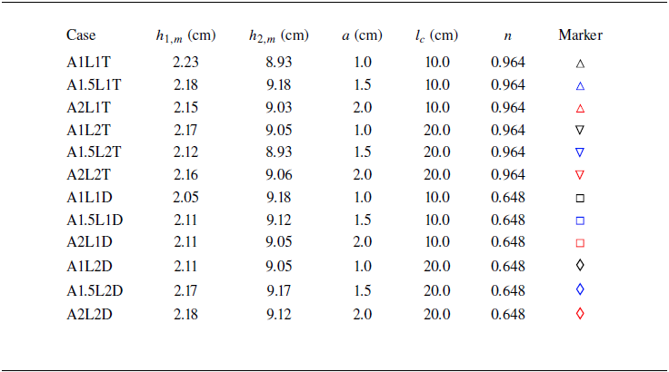


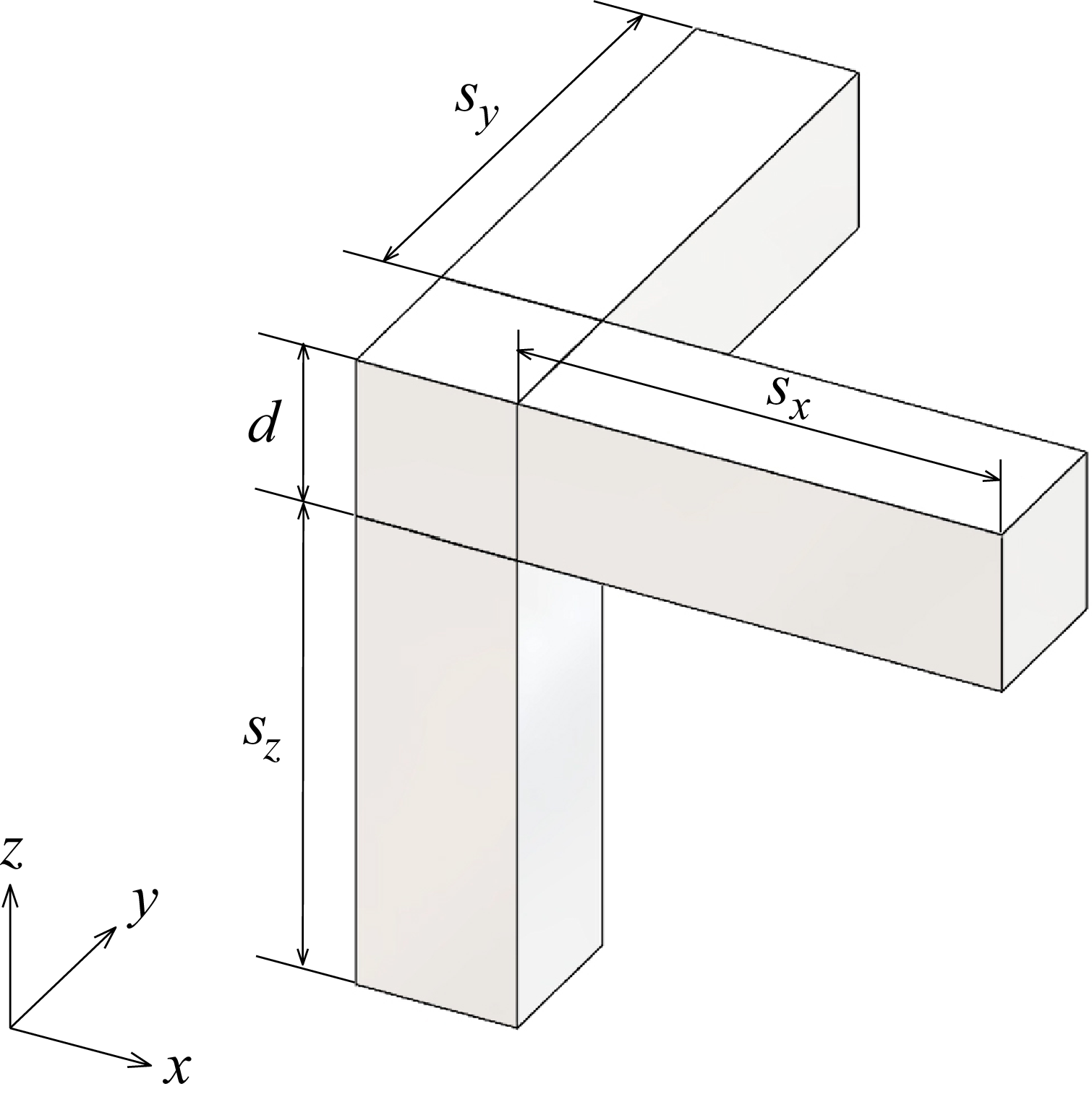

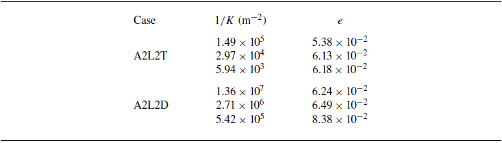

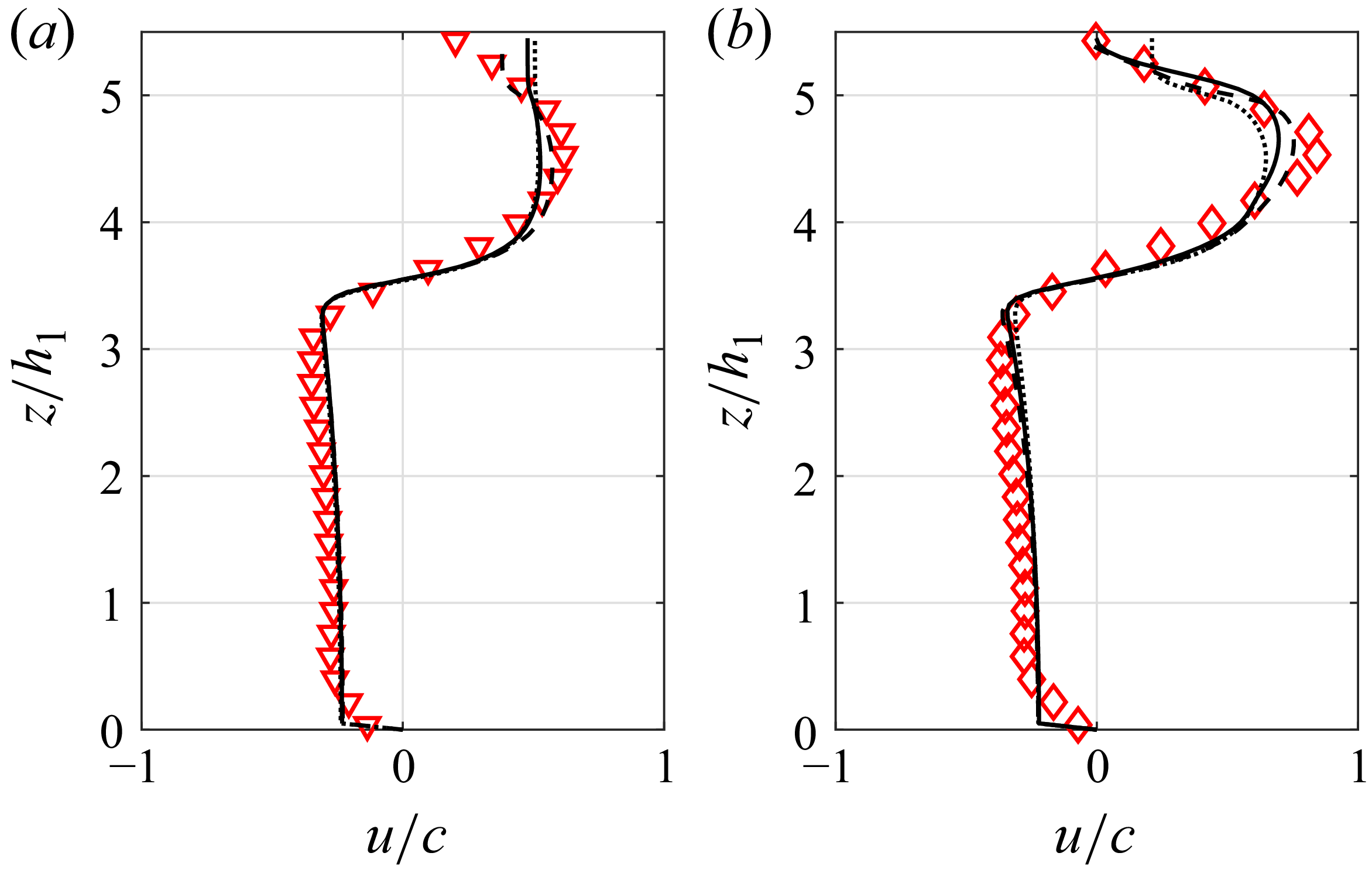


 Open access