





1. Introduction
Venus is comparable to Earth in terms of size, mass and internal composition. However, unlike Earth, Venus lacks an intrinsic global magnetic field, leaving its atmosphere unprotected from the solar wind, which is a continuous stream of charged particles emitted by the Sun. As a result, the upper layers of the Venus atmosphere, particularly the ionosphere, experience significant atmospheric loss because of direct exposure to this solar wind. The plasma environment of Venus is thus regulated by the joint influence of solar wind and solar radiation, leading to extensive ionisation, plasma instabilities and increased atmospheric loss, e.g. acceleration of ionospheric plasma into space like hydrogen and oxygen, because they are light ions. In the absence of an internal magnetic shield, Venus develops a weak induced magnetosphere. This external magnetic shielding arises from the interaction between the solar wind and the dense ionosphere of the planet. Specifically, the interplanetary magnetic field is draped around Venus by the solar-wind flow, and induced electric currents at the ionospheric boundary give rise to localised magnetic fields that partially mediate the solar-wind interaction (Spenner et al. Reference Spenner, Knudsen, Miller, Novak, Russell and Elphic1980; Futaana et al. Reference Futaana, Wieser, Gabriella and Luhmann2017).
The exploration and investigation of Venus are of profound relevance to our knowledge of planetary formation, climate and atmospheric processes, and are therefore an excellent research target for astronomers and planetary scientists alike (Taylor Jr et al. Reference Taylor, Brinton, Bauer, Hartle, Cloutier and Daniell1980; Luhmann Reference Luhmann1986; Bougher, Hunten & Phillips Reference Bougher, Hunten and Phillips2022). Several spacecraft missions, such as Venus Express (VEX) and Pioneer Venus Orbiter (PVO), have investigated the effect of the solar wind on the Venus atmosphere in depth (Luhmann et al. Reference Luhmann, Russell, Schwingenschuh and Yeroshenko1991; Mahajan & Dwivedi Reference Mahajan and Dwivedi2004; Barabash et al. Reference Barabash2007; Futaana et al. Reference Futaana, Wieser, Gabriella and Luhmann2017). Examples of space plasmas that often form collisionless media include ionospheres and magnetospheres. Consequently, other plasma regions gain energy and momentum through plasma waves. They are thus thought to be a crucial aspect of space plasmas. Because space plasma is often in non-thermal equilibrium or contains a significant quantity of free energy, waves have been shown to be widely used everywhere. One of several places in the planet’s environment where electrostatic solitary waves are seen is the magnetosheath (Strangeway Reference Strangeway1991; Pickett et al. Reference Pickett, Menietti, Gurnett, Tsurutani, Kintner, Klatt and Balogh2003). Plasma waves in the Venus mantle (between the magnetosheath and the lobe region) were detected by the Orbiter Electric Field Detector (OEFD) during the PVO mission. During the PVO flyby, several waves were seen, and it was found that the wave observations were in the 100 Hz channel and the Doppler-shifted ion-acoustic waves in the 730 Hz and 5.4 kHz channels. Current research increases the breadth and reliability of studies on wave phenomena in the Venus environment (Scarf et al. Reference Scarf, Taylor, Russell and Elphic1980b ; Strangeway Reference Strangeway1991; Futaana et al. Reference Futaana, Wieser, Gabriella and Luhmann2017; Yadav Reference Yadav2022; Kamalam et al. Reference Kamalam, Singh, Sreeraj and Lakhina2023; Rubia et al. Reference Rubia, Singh, Lakhina, Devanandhan, Dhanya and Kamalam2023).
In space plasma, holes are regions where there is a depletion in a specific physical quantity relative to the surrounding areas, such as a density hole, where the number of charged particles is significantly lower than in the surrounding plasma, and a magnetic hole, where the magnetic field is significantly lower than in the surrounding plasma. The electron hole in the phase space is a localised area of positive potential with an electron density lower than that of the surrounding plasma. This occurs as a result of the phase-space density being decreased by constrained electron orbits. A local maximum charge density is caused by a decrease in electron density, which increases the electric potential. This increased potential, in turn, enhances the trapping of electrons in a self-consistent manner, and this leads to the formation of solitary electrostatic waves in a bipolar parallel electric field (Schamel Reference Schamel1986; Franz et al. Reference Franz, Kintner, Pickett and Chen2005; Hutchinson Reference Hutchinson2017; Kuzichev et al. Reference Kuzichev, Agapitov, Mozer and Artemyev2017; Holmes et al. Reference Holmes, Ergun, Newman, Ahmadi, Andersson, Le Contel, Torbert, Giles, Strangeway and Burch2018; Hadid et al. Reference Hadid2021).
Ion-acoustic waves (IAWs) are important in the study of nonlinear phenomena such as turbulence and solitons when modelling complex plasma systems. These waves are low-frequency (relative to electrons) collective excitations that travel in the plasma medium because of the coupling between electron pressure and ionic inertia. The IAW mechanism is related to the restoring of charge neutrality in the plasma. When a small disturbance compresses the ions in a region, the electrons, since they are much more mobile, redistribute themselves instantaneously to shield the excess positive charge. Their thermal pressure, however, does not allow the shielding to be complete and generates an electrostatic field that pushes the heavier ions back towards equilibrium. This ion movement generates a propagating wave. The IAWs play a key role in numerous plasma processes, such as energy transfer, wave–particle interactions and both space and laboratory plasma dynamics. Electrostatic waves in situ detected by the Parker Solar Probe (PSP) in the mantle region of the Venus atmosphere propagate parallel to the magnetic field (with an average magnitude of $B\sim 100\,\mathrm{nT}$
) or, in its absence, along the local plasma direction (Lundin et al. Reference Lundin, Barabash, Futaana, Sauvaud, Fedorov and Perez-de Tejada2011; Knudsen et al. Reference Knudsen, Jones, Peterson, Knadler and Charles2016; Morsi et al. Reference Morsi, Fayad, Tolba, Fichtner, Lazar and Moslem2024). Parallel propagation with respect to the magnetic field implies that the field does not affect the longitudinal electrostatic structure of the waves, but influences only their transverse dynamics. Accordingly, we adopt a one-dimensional model in which the electrostatic wave propagates strictly parallel to the ambient magnetic field. This configuration has been reported in recent observational and theoretical studies (Hadid et al. Reference Hadid2021; Rubia et al. Reference Rubia, Singh, Lakhina, Devanandhan, Dhanya and Kamalam2023), providing further support for the validity of this assumption. In the parallel case, the magnetic field does not modify the longitudinal electrostatic dynamics, allowing us to neglect magnetic terms and focus on the fundamental wave behaviour. This simplification is appropriate for the cases analysed here, while the characteristics of magnetised or oblique propagation could be explored in future studies. Various wave phenomena, including 100 Hz electromagnetic whistler waves, 5.4 kHz Doppler-shifted electrostatic IAWs and 30 kHz Langmuir oscillations, have been observed in the Venus generated magnetosphere (Scarf, Taylor & Green Reference Scarf, Taylor and Green1979, Reference Scarf, Taylor, Russell and Elphic1980b
; Strangeway Reference Strangeway1991). A phase-space electron hole travelling parallel to the magnetic field is among them; it has a Doppler-shifted frequency of around 5.4 kHz and an electric field of about 15 mV m–1. These results demonstrate how intricate and unpredictable plasma interactions are in the Venus ionosphere (Malaspina et al. Reference Malaspina, Andersson, Ergun, Wygant, Bonnell, Kletzing, Reeves, Skoug and Larsen2014; Hadid et al. Reference Hadid2021; Rubia et al. Reference Rubia, Singh, Lakhina, Devanandhan, Dhanya and Kamalam2023).
$B\sim 100\,\mathrm{nT}$
) or, in its absence, along the local plasma direction (Lundin et al. Reference Lundin, Barabash, Futaana, Sauvaud, Fedorov and Perez-de Tejada2011; Knudsen et al. Reference Knudsen, Jones, Peterson, Knadler and Charles2016; Morsi et al. Reference Morsi, Fayad, Tolba, Fichtner, Lazar and Moslem2024). Parallel propagation with respect to the magnetic field implies that the field does not affect the longitudinal electrostatic structure of the waves, but influences only their transverse dynamics. Accordingly, we adopt a one-dimensional model in which the electrostatic wave propagates strictly parallel to the ambient magnetic field. This configuration has been reported in recent observational and theoretical studies (Hadid et al. Reference Hadid2021; Rubia et al. Reference Rubia, Singh, Lakhina, Devanandhan, Dhanya and Kamalam2023), providing further support for the validity of this assumption. In the parallel case, the magnetic field does not modify the longitudinal electrostatic dynamics, allowing us to neglect magnetic terms and focus on the fundamental wave behaviour. This simplification is appropriate for the cases analysed here, while the characteristics of magnetised or oblique propagation could be explored in future studies. Various wave phenomena, including 100 Hz electromagnetic whistler waves, 5.4 kHz Doppler-shifted electrostatic IAWs and 30 kHz Langmuir oscillations, have been observed in the Venus generated magnetosphere (Scarf, Taylor & Green Reference Scarf, Taylor and Green1979, Reference Scarf, Taylor, Russell and Elphic1980b
; Strangeway Reference Strangeway1991). A phase-space electron hole travelling parallel to the magnetic field is among them; it has a Doppler-shifted frequency of around 5.4 kHz and an electric field of about 15 mV m–1. These results demonstrate how intricate and unpredictable plasma interactions are in the Venus ionosphere (Malaspina et al. Reference Malaspina, Andersson, Ergun, Wygant, Bonnell, Kletzing, Reeves, Skoug and Larsen2014; Hadid et al. Reference Hadid2021; Rubia et al. Reference Rubia, Singh, Lakhina, Devanandhan, Dhanya and Kamalam2023).
A double-layer (DL) or shock-like structure in a plasma is the spontaneous formation of two parallel layers of opposite electrical charges, creating a localised electric field that has the capability to accelerate particles. They are spontaneously formed in a plasma under certain conditions and are responsible for the particle dynamics and energy transfer. Such DLs are usually considered as nonlinear phenomena and can serve as sources of strong electric fields controlling the motion of neighbouring plasma. Using the PSP, electrostatic ion-acoustic DLs were detected in the Venusian magnetosheath (Block Reference Block1978; Gołkowski et al. Reference Gołkowski, Harid and Hosseini2019; Malaspina et al. Reference Malaspina2020).
When hot and cold electron populations interact, fascinating plasma structures known as DLs are created. It has been suggested that the mixing of planetary cold electrons with electrons from the solar wind may activate these formations. Because it has the potential to accelerate or heat planetary cold electrons, this excitation process is important because it can affect the dynamics of the surrounding plasma. The contact between hot and cold plasma populations, which fosters the production of DLs, is one of the basic processes causing this excitation. For Venus in particular, these formations are thought to form in the transition zone where the colder planetary plasma interacts with the solar wind. Due to this special configuration, the two plasma populations could interact more easily, which activates DLs and may be important in determining how the plasma behaves close to the planet (Hultqvist Reference Hultqvist1971; Knorr & Goertz Reference Knorr and Goertz1974).
A solitary wave (SW) is a localised disturbance that arises from a delicate balance between nonlinear and dispersive effects, maintaining its shape while propagating at a constant speed. Such waves are generally encountered in plasmas and fluids, where nonlinearity tends to steepen the wave front and dispersion counteracts this tendency by spreading the wave energy. In planetary ionospheres, such as that of Venus, single waves have been suggested as key contributors to plasma dynamics. The ionosphere of Venus is significant in that it can provide some insights into ion outflow and drivers of atmospheric loss. The creation of solitary structures could be the cause of ion acceleration and transport outside the planet-created magnetosphere and could have a role in long-term atmospheric development on Venus (Rosenau Reference Rosenau1997; Akbari et al. Reference Akbari2022).
In this study, we advance the theoretical description of phase-space electron holes identified in the Venusian mantle, where electrons are confined within localised electrostatic structures, by incorporating the dynamics of trapped ionospheric electrons. To capture the departure of the electron population from a Boltzmann distribution, we adopt a Schamel-type trapping-compatible closure, which introduces modified nonlinear characteristics and supports the existence of both SW and DL solutions. The formulation accounts for the finite nonlinear contribution arising from weak trapping, thereby validating the application of the reductive perturbation method (Scarf et al. Reference Scarf, Taylor and Green1979; Malaspina et al. Reference Malaspina2020; Hadid et al. Reference Hadid2021). The purpose of this work is to investigate the influence of the solar wind on phase-space electron holes that govern the nonlinear evolution of IAWs at the upper mantle barrier, based on temperature, density and velocity measurements obtained by the VEX mission (Lundin et al. Reference Lundin, Barabash, Futaana, Sauvaud, Fedorov and Perez-de Tejada2011; Knudsen et al. Reference Knudsen, Jones, Peterson, Knadler and Charles2016). This treatment complements and extends the approach of Morsi et al. (Reference Morsi, Fayad, Tolba, Fichtner, Lazar and Moslem2024), in which they considered Maxwellian fluid electrons and therefore did not include electron-hole effects. Furthermore, the present normalisation, based on oxygen ion species and Venusian mantle temperatures, provides a physically consistent framework that differs from the hydrogen-based, isothermal model employed by Morsi et al. (Reference Morsi, Fayad, Tolba, Fichtner, Lazar and Moslem2024), which can be regarded as a limiting case of the more general approach developed here. While both studies employ a Zakharov–Kuznetsov-type formulation, the present model establishes a comprehensive and physically consistent framework for describing nonlinear plasma dynamics in the Venusian environment. The novelty of this work lies in its integration of solar-wind effects with Schamel-type electron trapping in a Venusian plasma context, offering new insights into the formation and evolution of electrostatic structures under realistic planetary conditions.
The structure of the work is arranged as follows. In § 2, we investigate the physical representation of our observations and the hydrodynamic model. In § 3, we evaluate our model using the perturbation method and a small percentage of non-isothermal electron distributions (Schamel distribution). While in § 4, our theoretical study’s numerical results are explained. Finally, § 5 presents a summary and conclusion.
2. Formulation of the problem
2.1. Physical representation and observations
Physical morphology and observational data of the mantle region of the Venus ionosphere are important in the mediation of solar wind and planetary plasma interaction. The mantle has been described as an intermediate region between the magnetosheath and the ionosphere with a varying electron energy distribution from planetary to solar wind (Futaana et al. Reference Futaana, Wieser, Gabriella and Luhmann2017).
Despite the importance of this planet, few space missions, such as PVO (Colin Reference Colin1980) and VEX (Titov et al. Reference Titov2006), were equipped with plasma wave detectors. The OEFD on PVO has poor frequency resolution, and wave modes are not easily detectable (Scarf et al. Reference Scarf, Taylor, Russell and Elphic1980b ). Despite the other explanations offered (e.g. whistler waves, lower hybrid waves or IAWs), more recent theory and observations identify IAWs as the leading candidate for wave activity observations (Scarf et al. Reference Scarf, Taylor, Russell and Elphic1980b ; Huba Reference Huba1993; Strangeway & Crawford Reference Strangeway and Crawford1993). Although Venusian IAW observations are important, we need more high-resolution missions to keep monitoring these waves and the role they play in solar wind–Venusian ionosphere energy and momentum transfer. So we study IAWs (SWs and DLs) to know how the solar wind affects the environmental plasma.
2.2. Theoretical model
This paper examines the propagation of electrostatic ion-acoustic excitations through the Venusian mantle. To do so, we use a hydrodynamic model of a one-dimensional, collisionless plasma that includes two adiabatic, positively charged planetary ions, namely hydrogen (subscript $H^+$
) and oxygen (subscript
$H^+$
) and oxygen (subscript $O^+$
), as well as streaming solar-wind protons (subscript
$O^+$
), as well as streaming solar-wind protons (subscript $sp$
). Our model also incorporates inertialess solar-wind thermal and superthermal (Kappa-distributed) electrons (subscripts
$sp$
). Our model also incorporates inertialess solar-wind thermal and superthermal (Kappa-distributed) electrons (subscripts $se$
and
$se$
and $ke$
, respectively), as well as inertialess, free and trapped planetary electrons (subscripts
$ke$
, respectively), as well as inertialess, free and trapped planetary electrons (subscripts $\textit{fe}$
and
$\textit{fe}$
and $te$
).
$te$
).
The continuity and the momentum equations of the ionic species ( $j=O^+, H^+, sp$
) are given by
$j=O^+, H^+, sp$
) are given by
 \begin{align} & \frac {\partial n_j}{\partial t}+\frac {\partial (n_j u_j)}{\partial x} = 0, \nonumber\\[5pt]& \frac {\partial u_j}{\partial t}+u_j \frac {\partial u_j}{\partial x} +\rho _j \frac {\partial \phi }{\partial x} +3 \sigma _j \rho _j n_j \frac {\partial n_j}{\partial x} = 0, \end{align}
where $\sigma _j=T_j/T_{\textit{eff}}$
is the ratio between the
$\sigma _j=T_j/T_{\textit{eff}}$
is the ratio between the $j$
species temperature
$j$
species temperature $T_j$
and the effective electron temperature
$T_j$
and the effective electron temperature $T_{\textit{eff}}$
, and
$T_{\textit{eff}}$
, and $\rho _{j}=m_{O^+}/m_j$
is the mass ratio between the
$\rho _{j}=m_{O^+}/m_j$
is the mass ratio between the $O^+$
and the
$O^+$
and the $j$
species.
$j$
species.
The ionospheric electrons are assumed to be inertialess and consist of a small percentage of non-isothermal trapped electrons (subscript ‘ $te$
’) and isothermal electrons (subscript ‘
$te$
’) and isothermal electrons (subscript ‘ $\textit{fe}$
’) (Schamel Reference Schamel1973; Das, Paul & Karmakar Reference Das, Paul and Karmakar1986):
$\textit{fe}$
’) (Schamel Reference Schamel1973; Das, Paul & Karmakar Reference Das, Paul and Karmakar1986):
 \begin{equation} n_e=\text{exp}{(\phi /\sigma _{\textit{fe}})}-\frac {4}{3}b\left (\phi /\sigma _{te}\right )^{ {3}/{2}}, \end{equation}
with
 \begin{align} b & = \frac {1}{\sqrt \pi }(1-\beta),\quad \beta =\frac {T_{\textit{fe}}}{T_{te}} , \quad \sigma _{\textit{fe}}=\frac {T_{\textit{fe}}}{T_{\textit{eff}}},\quad \sigma _{te}=\frac {T_{te}}{T_{\textit{eff}}},\\[-10pt]\nonumber \end{align}
 \begin{align} T_{\textit{eff}} & = \frac {T_{\textit{fe}} T_{ke}T_{se}\left (\kappa -{3}/{2}\right )}{\mu \left (\kappa -{3}/{2}\right )T_{ke} T_{se}+\omega \left (\kappa -{1}/{2}\right )T_{\textit{fe}} T_{se}+\delta \left (\kappa -{3}/{2}\right )T_{\textit{fe}} T_{ke}}, \end{align}
where $b$
is the trapped electron coefficient,
$b$
is the trapped electron coefficient, $\beta$
is the temperature ratio between the free and trapped electrons,
$\beta$
is the temperature ratio between the free and trapped electrons, $\sigma _{\textit{fe}}$
is the temperature ratio between the free and effective electrons and
$\sigma _{\textit{fe}}$
is the temperature ratio between the free and effective electrons and $\sigma _{te}$
is the temperature ratio between the trapped and effective electrons. The investigation of phase-space electron holes, wherein electrons are confined within a localised region, requires that the fraction of trapped electrons remains significantly smaller than the total electron population. This constraint is quantified by the trapped coefficient
$\sigma _{te}$
is the temperature ratio between the trapped and effective electrons. The investigation of phase-space electron holes, wherein electrons are confined within a localised region, requires that the fraction of trapped electrons remains significantly smaller than the total electron population. This constraint is quantified by the trapped coefficient $b$
, which characterises the degree of electron trapping and dictates how the flattening, depletion or enhancement of the trapped electron distribution influences the effective nonlinearity of the system. In the reductive perturbation expansion we treat the temperature ratios
$b$
, which characterises the degree of electron trapping and dictates how the flattening, depletion or enhancement of the trapped electron distribution influences the effective nonlinearity of the system. In the reductive perturbation expansion we treat the temperature ratios $\beta =T_{\textit{fe}}/T_{te}$
and
$\beta =T_{\textit{fe}}/T_{te}$
and $\sigma _{O}$
as
$\sigma _{O}$
as $O(1)$
and therefore do not expand them in
$O(1)$
and therefore do not expand them in $\varepsilon$
. The trapping parameter
$\varepsilon$
. The trapping parameter $b$
originates from the Schamel distribution and quantifies the trapped-population fraction; its ordering is chosen to balance nonlinearities. With the standard Korteweg de Vries (KdV) stretching
$b$
originates from the Schamel distribution and quantifies the trapped-population fraction; its ordering is chosen to balance nonlinearities. With the standard Korteweg de Vries (KdV) stretching $\phi \sim \varepsilon$
,
$\phi \sim \varepsilon$
, $\partial _{\xi }\sim \varepsilon ^{1/2}$
,
$\partial _{\xi }\sim \varepsilon ^{1/2}$
, $\partial _{\tau }\sim \varepsilon ^{3/2}$
, the convective term scales as
$\partial _{\tau }\sim \varepsilon ^{3/2}$
, the convective term scales as $\phi \,\phi _{\xi }=O(\varepsilon ^{3/2})$
(Washimi & Taniuti Reference Washimi and Taniuti1966). We therefore order
$\phi \,\phi _{\xi }=O(\varepsilon ^{3/2})$
(Washimi & Taniuti Reference Washimi and Taniuti1966). We therefore order $b$
so that the trapping nonlinearity (e.g.
$b$
so that the trapping nonlinearity (e.g. $b\,|\phi |\,\phi _{\xi }$
, or in closures yielding
$b\,|\phi |\,\phi _{\xi }$
, or in closures yielding $b\,|\phi |^{1/2}\phi _{\xi }$
take
$b\,|\phi |^{1/2}\phi _{\xi }$
take $b\sim \varepsilon ^{1/2}$
) enters at the same asymptotic order, producing a Schamel–KdV equation rather than a standard KdV equation (Schamel Reference Schamel1972). If
$b\sim \varepsilon ^{1/2}$
) enters at the same asymptotic order, producing a Schamel–KdV equation rather than a standard KdV equation (Schamel Reference Schamel1972). If $b$
is ordered smaller, the trapping term drops out at leading order; if larger, the KdV-type balance is lost. Thus, smallness is attributed to the trapped population (
$b$
is ordered smaller, the trapping term drops out at leading order; if larger, the KdV-type balance is lost. Thus, smallness is attributed to the trapped population ( $b$
), not to the temperature ratios themselves. On the other hand, the scaling of
$b$
), not to the temperature ratios themselves. On the other hand, the scaling of $b \sim \varepsilon ^{1/2}$
is to include both the nonlinear terms, the results from the trapping and the convective term, in the final evolution equation. Otherwise, we obtain a usual KdV equation without incorporating the trapping effect (Das & Tagare Reference Das and Tagare1975; Das Reference Das1979; Das et al. Reference Das, Paul and Karmakar1986). Under the assumption of a weak electrostatic potential amplitude, the reductive perturbation technique is applied to the governing hydrodynamic equations, ultimately yielding the Schamel–KdV equation (Schamel Reference Schamel1972).
$b \sim \varepsilon ^{1/2}$
is to include both the nonlinear terms, the results from the trapping and the convective term, in the final evolution equation. Otherwise, we obtain a usual KdV equation without incorporating the trapping effect (Das & Tagare Reference Das and Tagare1975; Das Reference Das1979; Das et al. Reference Das, Paul and Karmakar1986). Under the assumption of a weak electrostatic potential amplitude, the reductive perturbation technique is applied to the governing hydrodynamic equations, ultimately yielding the Schamel–KdV equation (Schamel Reference Schamel1972).
Observations from multiple spacecraft, including Helios, Ulysses, Cluster II and PSP (Štverák et al. Reference Štverák, Trávníček, Maksimovic, Marsch, Fazakerley and Scime2008; Abraham et al. Reference Abraham2022; Shaaban et al. Reference Shaaban, Kennis, Lazar, Pierrard and Poedts2025), indicate that solar-wind electrons exhibit a dual velocity distribution, consisting of a cool, dense thermal core with number density $n_{se}$
and a hotter, more dilute suprathermal halo with number density
$n_{se}$
and a hotter, more dilute suprathermal halo with number density $n_{ke}$
. These two populations are well described by a Maxwellian (Boltzmann) distribution for the core,
$n_{ke}$
. These two populations are well described by a Maxwellian (Boltzmann) distribution for the core,
 \begin{align} n_{se}=\text{exp}{\left (\phi \right /\!\sigma _{se})}, \end{align}
and a Kappa distribution for the halo,
 \begin{equation} n_{ke}=\left [1-\frac {\phi /\sigma _{ke}}{\left (\kappa -3/2\right )}\right ]^{-\kappa + {1}/{2}}, \end{equation}
respectively (Afify et al. Reference Afify, Elkamash, Shihab and Moslem2021), where the total solar-wind electron number density is given by $n_W=n_{se}+n_{ke}$
,
$n_W=n_{se}+n_{ke}$
, $\sigma _{se}=T_{se}/T_{\textit{eff}}$
is the ratio of the solar-wind thermal electron to the effective electron temperatures,
$\sigma _{se}=T_{se}/T_{\textit{eff}}$
is the ratio of the solar-wind thermal electron to the effective electron temperatures, $\sigma _{ke}=T_{ke}/T_{\textit{eff}}$
is the ratio of the solar-wind suprathermal electron to the effective electron temperatures and
$\sigma _{ke}=T_{ke}/T_{\textit{eff}}$
is the ratio of the solar-wind suprathermal electron to the effective electron temperatures and $\kappa \in [3/2, \infty ]$
is the Kappa power index.
$\kappa \in [3/2, \infty ]$
is the Kappa power index.
The set of equations (2.1)–(2.5) is completed by the Poisson equation:
 \begin{align} \frac {\partial ^2\phi }{\partial x^2}=\mu n_{e}+{\omega n}_{ke}+\delta n_{se}-\psi n_{sp}-\alpha n_{H^+}-n_{O^+}, \end{align}
where $\mu =n_{te}^{(0)}/n_{O^+}^{(0)}$
,
$\mu =n_{te}^{(0)}/n_{O^+}^{(0)}$
, $\omega =n_{ke}^{(0)}/n_{O^+}^{(0)}$
,
$\omega =n_{ke}^{(0)}/n_{O^+}^{(0)}$
, $\delta =n_{se}^{(0)}/n_{O^+}^{(0)}$
,
$\delta =n_{se}^{(0)}/n_{O^+}^{(0)}$
,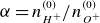 $\alpha =n_{H^+}^{(0)}/n_{O^+}^{(0)}$
and
$\alpha =n_{H^+}^{(0)}/n_{O^+}^{(0)}$
and $\psi =n_{sp}^{(0)}/n_{O^+}^{(0)}$
.
$\psi =n_{sp}^{(0)}/n_{O^+}^{(0)}$
.
It is worth noting that the physical quantities in (2.1)–(2.6), i.e. $n_j$
,
$n_j$
, $u_i$
,
$u_i$
, $\phi$
,
$\phi$
, $x$
,
$x$
, $t$
, are normalised by using the unperturbed density
$t$
, are normalised by using the unperturbed density $n_j^{(0)}$
of the
$n_j^{(0)}$
of the $j$
th species, ion-acoustic speed
$j$
th species, ion-acoustic speed $c_{sO^+}=\sqrt {k_BT_{\textit{eff}}/m_{O^+}}$
, the electrostatic potential
$c_{sO^+}=\sqrt {k_BT_{\textit{eff}}/m_{O^+}}$
, the electrostatic potential $k_BT_{\textit{eff}}/e$
, the inverse of the effective Debye length
$k_BT_{\textit{eff}}/e$
, the inverse of the effective Debye length $\lambda _D ^{-1}=\sqrt {n_{O^+}^{(0)} e^2/\epsilon _0 k_BT_{\textit{eff}}}$
, the ion plasma frequency
$\lambda _D ^{-1}=\sqrt {n_{O^+}^{(0)} e^2/\epsilon _0 k_BT_{\textit{eff}}}$
, the ion plasma frequency ${\omega _{pO^+}}=\,\sqrt {n_{O^+}^{(0)} e^2/\epsilon _0 m_{O^+}}$
,
${\omega _{pO^+}}=\,\sqrt {n_{O^+}^{(0)} e^2/\epsilon _0 m_{O^+}}$
, $\lambda _D / c_{sO^+}=1/\omega _{pO^+}$
, where
$\lambda _D / c_{sO^+}=1/\omega _{pO^+}$
, where $j$
refers to plasma species (
$j$
refers to plasma species ( $H^+$
,
$H^+$
, $O^+$
,
$O^+$
, $e$
,
$e$
, $sp$
,
$sp$
, $ke$
),
$ke$
), $i$
refers to plasma species (
$i$
refers to plasma species ( $H^+$
,
$H^+$
, $O^+$
,
$O^+$
, $sp$
),
$sp$
), $k_B$
is the Boltzmann constant and
$k_B$
is the Boltzmann constant and $e$
is the electron charge. Oxygen is the dominant ion in the studied altitude range; therefore, normalisation is based on its acoustic speed and effective Debye length. Under this scheme, waves can appear either subsonic or supersonic, consistent with observations. In comparison, hydrogen-based normalisation yields
$e$
is the electron charge. Oxygen is the dominant ion in the studied altitude range; therefore, normalisation is based on its acoustic speed and effective Debye length. Under this scheme, waves can appear either subsonic or supersonic, consistent with observations. In comparison, hydrogen-based normalisation yields $U \lt 1$
, making all waves appear subsonic (Sayed et al. Reference Sayed, Turky, Koramy and Moslem2020).
$U \lt 1$
, making all waves appear subsonic (Sayed et al. Reference Sayed, Turky, Koramy and Moslem2020).
3. The evolution equation
The essential characteristics of small but finite-amplitude IAWs are investigated using the reductive perturbation method (Washimi & Taniuti Reference Washimi and Taniuti1966). We introduce the extended space–time transformation $\xi =\varepsilon ^{ {1}/{2}} (x-\lambda t)$
and
$\xi =\varepsilon ^{ {1}/{2}} (x-\lambda t)$
and $\tau =\varepsilon ^{ {3}/{2}} t$
, where
$\tau =\varepsilon ^{ {3}/{2}} t$
, where $\lambda$
is the linear phase velocity normalised to
$\lambda$
is the linear phase velocity normalised to $c_{sO^+}$
and
$c_{sO^+}$
and $\varepsilon$
is a small parameter characterising the smallness of the amplitude or dispersion of the nonlinear modes. The normalised physical quantities
$\varepsilon$
is a small parameter characterising the smallness of the amplitude or dispersion of the nonlinear modes. The normalised physical quantities $n_j$
,
$n_j$
, $u_i$
and
$u_i$
and $\phi$
are extended around their equilibrium values in the power series of
$\phi$
are extended around their equilibrium values in the power series of $\varepsilon$
as
$\varepsilon$
as
 \begin{align} n_j & = 1+\varepsilon n_j^{(1)}+\varepsilon ^2 n_j^{\left (2\right )}+\varepsilon ^3 n_j^{\left (3\right )}+\cdots\! ,\\[-10pt]\nonumber \end{align}
 \begin{align} u_i & = \varepsilon u_i^{(1)}+\varepsilon ^2 u_i^{\left (2\right )}+\varepsilon ^3 u_i^{\left (3\right )}+\cdots\! ,\\[-10pt]\nonumber \end{align}
 \begin{align} u_{sp} & = u_{sp}^{\left (0\right )}+\varepsilon u_{sp}^{(1)}+\varepsilon ^2 u_{sp}^{\left (2\right )}+\varepsilon ^3 u_{sp}^{\left (3\right )}+\cdots\! ,\\[-10pt]\nonumber \end{align}
 \begin{align} \phi & = \varepsilon \phi ^{(1)}+\varepsilon ^2\phi ^{(2)}+\varepsilon ^3\phi ^{(3)}+\cdots\! . \end{align}
Theoretically, IAWs in plasmas are explained by the Schamel–KdV equation, especially when electron trapping is significant. Non-isothermality in this scenario is a description for departures from the isothermality assumption; i.e. the situation in which electron temperature is assumed to be constant. It involves the introduction of a small percentage of non-isothermality to explain small changes in thermal properties occurring due to the existence of both free (Maxwellian) and confined electron species. The Schamel distribution finds application in the case of consideration of electrostatic potentials with small amplitudes. Ion-acoustic waves are generated because of the disturbance of the plasma species around an equilibrium state. These disturbances are mainly generated by the perturbation in number densities, fluid velocities and electrostatic potential. As a result, in our model, we took into account the change of fluid of the plasma species. We take a small percentage of trapped electrons $b=\acute {b}\varepsilon ^{{1}/{2}}$
and apply the stretching space–time coordinates and expansion equations (3.1) to fluid equations (2.1)–(2.6). The lowest-order equations in
$b=\acute {b}\varepsilon ^{{1}/{2}}$
and apply the stretching space–time coordinates and expansion equations (3.1) to fluid equations (2.1)–(2.6). The lowest-order equations in $\varepsilon$
include (Das et al. Reference Das, Paul and Karmakar1986; El-Labany, El-Warraki & Moslem Reference El-Labany, El-Warraki and Moslem2000)
$\varepsilon$
include (Das et al. Reference Das, Paul and Karmakar1986; El-Labany, El-Warraki & Moslem Reference El-Labany, El-Warraki and Moslem2000)
 \begin{align} u_{O^+}^{(1)} & = \frac {\lambda \phi ^{(1)}}{\lambda ^2-3\sigma _{O^+}}, \quad n_{O^+}^{(1)}=\frac {\phi ^{(1)}}{\lambda ^2-3\sigma _{O^+}},\\[-10pt]\nonumber \end{align}
 \begin{align} u_{H^+}^{(1)} & = \frac {\lambda \rho _{H^+}\phi ^{(1)}}{\lambda ^2-3\sigma _{H^+}\rho _{H^+}} ,\quad n_H^{(1)}=\frac {\rho _{H^+}\phi ^{(1)}}{\lambda ^2-3\sigma _{H^+}\rho _{H^+}},\\[-10pt]\nonumber \end{align}
 \begin{align} u_{sp}^{(1)} & = \frac {\big(\lambda -u_{sp}^{(0)}\big)\rho _{sp}\phi ^{(1)}}{\big(\lambda -u_{sp}^{(0)}\big)^2-3\sigma _{sp}\rho _{sp}},\quad n_{sp}^{(1)}=\frac {\rho _{sp}\phi ^{(1)}}{\big(\lambda -u_{sp}^{(0)}\big)^2-3\sigma _{sp}\rho _{sp}},\\[-10pt]\nonumber \end{align}
 \begin{align} n_e^{(1)} & = \phi ^{(1)}/\sigma _{\textit{fe}},\\[-10pt]\nonumber \end{align}
 \begin{align} n_{se}^{(1)} & = \phi ^{(1)}/\sigma _{se},\\[-10pt]\nonumber \end{align}
 \begin{align} n_{ke}^{(1)} & = \frac {(\kappa -1/2)}{(\kappa -3/2)}\frac {\phi ^{(1)}}{\sigma _{ke}}. \end{align}
The Poisson equation (2.6) gives the compatibility condition as
 \begin{align} \frac {\mu }{\sigma _{\textit{fe}}} & +\frac {\omega }{\sigma _{ke}}\left (\frac {\kappa -1/2}{\kappa -3/2}\right )+\frac {\delta }{\sigma _{se}} \nonumber\\[3pt]& -\frac {\psi \rho _{sp}}{\big(\lambda -u_{sp}^{(0)}\big)^2-3\sigma _{sp}\rho _{sp}}-\frac {\alpha \rho _{H^+}}{\lambda ^2-3\sigma _{H^+}\rho _{H^+}}-\frac {1}{\lambda ^2-3\sigma _{O^+}}=0. \end{align}
Extending the perturbation expansion to higher orders of $\varepsilon$
yields a set of equations that characterise the dynamics of the second-order perturbed quantities. To solve this system, we utilise the framework provided by (3.2), which enables the systematic derivation of the Schamel–KdV equation for electrostatic potential:
$\varepsilon$
yields a set of equations that characterise the dynamics of the second-order perturbed quantities. To solve this system, we utilise the framework provided by (3.2), which enables the systematic derivation of the Schamel–KdV equation for electrostatic potential:
 \begin{equation} \frac {\partial \phi }{\partial \tau }+\big[\acute {C}\sqrt \phi +\acute {A}\ \phi \big]\frac {\partial \phi }{\partial \xi }\ +D\frac {\partial ^3\phi }{\partial \xi ^3}=0,\ \end{equation}
where $\acute {C}=CD, \ \acute {A}=DA$
,
$\acute {C}=CD, \ \acute {A}=DA$
, $A$
and
$A$
and $C$
are the coefficients of the nonlinearity and
$C$
are the coefficients of the nonlinearity and $D$
is the coefficient of the dispersion, defined as
$D$
is the coefficient of the dispersion, defined as
 \begin{align} A & = \frac {3\psi {\rho _{sp}}^2\big[\big(\lambda -u_{sp}^{(0)}\big)^2+\sigma _{sp}\rho _{sp}\big]}{\big[\big(\lambda -u_{sp}^{(0)}\big)^2-3\sigma _{sp}\rho _{sp}\big]^3}+\frac {3\lambda ^2+3\sigma _{O^+}}{\left (\lambda ^2-3\sigma _{O^+}\right )^3}+\alpha \frac {3\lambda ^2{\rho _{H^+}}^2+3\sigma _{H^+}{\rho _{H^+}}^3}{\left (\lambda ^2-3\sigma _{H^+}\rho _{H^+}\right )^3}\nonumber \\[4pt]& \quad -\frac {\mu }{\sigma _{\textit{fe}}^2}-\frac {\omega }{\sigma _{ke}^2}\frac {\left (\kappa - {1}/{2}\right )\left (\kappa + {1}/{2}\right )}{\left (\kappa -{3}/{2}\right )^2}-\frac {\delta }{{\sigma _{se}^2}},\\[-6pt]\nonumber \end{align}
 \begin{align} C & = 2\mu \,b\,\sigma _{te}^{-3/2},\\[-6pt]\nonumber \end{align}
 \begin{align} \frac {1}{D} & = \frac {2\left (\lambda -u_{sp}^{(0)}\right )\rho _{sp}\psi }{\big[\big(\lambda -u_{sp}^{(0)}\big)^2-3\sigma _{sp}\rho _{sp}\big]^2}+\frac {2\lambda }{\left (\lambda ^2-3\sigma _{O^+}\right )^2}+\frac {2\lambda \rho _{H^+}\alpha }{\left (\lambda ^2-3\sigma _{H^+}\rho _{H^+}\right )^2}. \end{align}
The nonlinearity and dispersion in the Schamel–KdV equation play a crucial role in understanding the evolution of IAWs. To obtain the analytical solutions of the Schamel–KdV equation, we use travelling-wave transformation $\eta = \xi - U \tau$
which transforms the nonlinear partial differential equation into an ordinary differential equation in terms of
$\eta = \xi - U \tau$
which transforms the nonlinear partial differential equation into an ordinary differential equation in terms of $\eta$
, corresponding to stationary-wave structures in a frame moving with velocity, where
$\eta$
, corresponding to stationary-wave structures in a frame moving with velocity, where $U$
is the normalised propagation speed of the nonlinear wave in the co-moving frame in which the structure is stationary. This equation is integrated by applying the appropriate boundary condition
$U$
is the normalised propagation speed of the nonlinear wave in the co-moving frame in which the structure is stationary. This equation is integrated by applying the appropriate boundary condition $\phi (\eta )= {\rm d}\phi /{\rm d}\eta = {\rm d}^2\phi /{\rm d}\eta ^2 =0$
at
$\phi (\eta )= {\rm d}\phi /{\rm d}\eta = {\rm d}^2\phi /{\rm d}\eta ^2 =0$
at $\eta \rightarrow \pm \infty$
, from which we get the solitary solution. The electrostatic potential due to the localised solitary solution of (3.4) is given by (Tagare & Chakrabarti Reference Tagare and Chakrabarti1974; Das Reference Das1979; Dönmez & Dağhan Reference Dönmez and Dağhan2017)
$\eta \rightarrow \pm \infty$
, from which we get the solitary solution. The electrostatic potential due to the localised solitary solution of (3.4) is given by (Tagare & Chakrabarti Reference Tagare and Chakrabarti1974; Das Reference Das1979; Dönmez & Dağhan Reference Dönmez and Dağhan2017)
 \begin{equation} \phi _s=\left [\frac {4CD}{15U}+\sqrt {\frac {16C^2D^2}{225U^2}+\frac {AD}{3U}}\cosh {\left (\sqrt {\frac {U}{4D}}\ \eta \right )}\ \right ]^{-2}. \end{equation}
The electric field $E_s$
associated with SWs from (3.6) is given by
$E_s$
associated with SWs from (3.6) is given by
 \begin{equation} E_s=-\frac {\sqrt {{U}/{D}} \sqrt {({A D}/{3 U})+ ({16 C^2 D^2}/{225 U^2})} \sinh \left (({1}/{2}) \eta \sqrt {{U}/{D}}\right )}{\big[\sqrt {({A D}/{3 U})+ {16 C^2 D^2}/{225 U^2}} \cosh \left (({1}/{2}) \eta \sqrt {{U}/{D}}\right )+{4 C D}/{15 U}\big]^3}. \end{equation}
When we apply the appropriate boundary conditions $V(\phi )={\rm d}V/{\rm d}\phi =0,$ ${\rm d}V^2/{\rm d}^2\phi \lt 0$
at
${\rm d}V^2/{\rm d}^2\phi \lt 0$
at $\phi =\phi _{max}= 4{C}^2{A}^{-2}/25$
, we will get the DLs. The electrostatic potential due to the DL solution of (3.4) is given by (Das Reference Das1979; Das et al. Reference Das, Paul and Karmakar1986; Dönmez & Dağhan Reference Dönmez and Dağhan2017; Soliman, Zahran & Elkamash Reference Soliman, Zahran and Elkamash2023)
$\phi =\phi _{max}= 4{C}^2{A}^{-2}/25$
, we will get the DLs. The electrostatic potential due to the DL solution of (3.4) is given by (Das Reference Das1979; Das et al. Reference Das, Paul and Karmakar1986; Dönmez & Dağhan Reference Dönmez and Dağhan2017; Soliman, Zahran & Elkamash Reference Soliman, Zahran and Elkamash2023)
 \begin{equation} \phi _D=\ \frac {4{C}^2}{25{A}^2}\left [1-\tanh \left ({\eta }{\sqrt {\frac {U}{16D}}}\right )\right ]^2\!. \end{equation}
The corresponding electric field $E_D$
reads
$E_D$
reads
 \begin{equation} E_D=-\frac {2\sqrt {U}{C}^2}{25\sqrt {D}{A}^2}\left [1-\tanh \left ({\eta }{\sqrt {\frac {U}{16D}}}\right )\right ] \text{sech}^2\left ({\eta }{\sqrt {\frac {U}{16D}}}\right )\!. \end{equation}
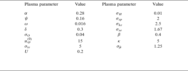
Plasma parameters used in the SW analysis.

Plasma parameters used in the DL analysis.
4. Numerical analysis and discussion
In this section, we investigate the propagation characteristics of IAWs at the upper mantle boundary of Venus and compare them with observed electrostatic structures. The analysis is conducted using plasma parameters adopted from in situ measurements by the VEX spacecraft (Lundin et al. Reference Lundin, Barabash, Futaana, Sauvaud, Fedorov and Perez-de Tejada2011; Knudsen et al. Reference Knudsen, Jones, Peterson, Knadler and Charles2016). The relevant plasma parameters are summarised in tables 1–3, covering SW (table 1) and DL (table 2) cases, as well as the observed plasma parameters, their corresponding normalised quantities and their effects on the electrostatic solutions (table 3). We note that the adopted value $\kappa = 5$
is consistent with in situ solar-wind observations. The Kappa index decreases with heliocentric distance, with electron distributions approaching Maxwellian conditions (large
$\kappa = 5$
is consistent with in situ solar-wind observations. The Kappa index decreases with heliocentric distance, with electron distributions approaching Maxwellian conditions (large $\kappa$
) closer to the Sun and exhibiting stronger suprathermal tails (smaller
$\kappa$
) closer to the Sun and exhibiting stronger suprathermal tails (smaller $\kappa$
) farther out. Typical inner heliospheric values lie in the range
$\kappa$
) farther out. Typical inner heliospheric values lie in the range $\kappa \sim 3{-}7$
(e.g. Maksimovic et al. (Reference Maksimovic2005), Lazar et al. (Reference Lazar, Pierrard, Poedts and Fichtner2020)), with values near the Venus orbit (
$\kappa \sim 3{-}7$
(e.g. Maksimovic et al. (Reference Maksimovic2005), Lazar et al. (Reference Lazar, Pierrard, Poedts and Fichtner2020)), with values near the Venus orbit ( ${\sim} 0.72$
AU) typically
${\sim} 0.72$
AU) typically $\kappa \approx 4{-}6$
.
$\kappa \approx 4{-}6$
.
The observed and normalised (norm.) values of plasma parameters obtained from VEX missions in the Venus ionosphere (Lundin et al. Reference Lundin, Barabash, Futaana, Sauvaud, Fedorov and Perez-de Tejada2011; Knudsen et al. Reference Knudsen, Jones, Peterson, Knadler and Charles2016) and their effects on the electrostatic waves.

We analyse two types of nonlinear electrostatic structures, namely SWs and DLs. Using the compatibility condition given in (3.3), we identify six distinct roots, each corresponding to a separate phase-velocity mode, denoted by $\lambda$
. The existence of multiple distinct roots implies the presence of multiple propagation modes, each associated with a specific species or interaction dynamic in the plasma. In figure 1, we examine the variation of the phase velocities, represented by the roots
$\lambda$
. The existence of multiple distinct roots implies the presence of multiple propagation modes, each associated with a specific species or interaction dynamic in the plasma. In figure 1, we examine the variation of the phase velocities, represented by the roots $\lambda _{1-6}$
, as functions of the hydrogen density ratio
$\lambda _{1-6}$
, as functions of the hydrogen density ratio $\alpha$
(top panel). Among the six modes, four are forward-propagating (
$\alpha$
(top panel). Among the six modes, four are forward-propagating ( $\lambda \gt 0$
), labelled as
$\lambda \gt 0$
), labelled as $\lambda _{3}$
to
$\lambda _{3}$
to $\lambda _{6}$
, and two are backward-propagating (
$\lambda _{6}$
, and two are backward-propagating ( $\lambda \lt 0$
), labelled as
$\lambda \lt 0$
), labelled as $\lambda _1$
and
$\lambda _1$
and $\lambda _2$
. The classification of these modes is based on the mass and initial velocity of the plasma species involved. The faster modes correspond to lighter species, whereas the slower modes correspond to heavier species. Accordingly,
$\lambda _2$
. The classification of these modes is based on the mass and initial velocity of the plasma species involved. The faster modes correspond to lighter species, whereas the slower modes correspond to heavier species. Accordingly, $\lambda _2$
and
$\lambda _2$
and $\lambda _3$
are attributed to planetary oxygen ions,
$\lambda _3$
are attributed to planetary oxygen ions, $\lambda _1$
and
$\lambda _1$
and $\lambda _4$
to planetary hydrogen ions and
$\lambda _4$
to planetary hydrogen ions and $\lambda _5$
and
$\lambda _5$
and $\lambda _6$
to solar-wind protons. Notably, both oxygen and hydrogen ions exhibit forward and backward modes. The bottom panels of figure 1 illustrate the variation of phase velocities for oxygen (
$\lambda _6$
to solar-wind protons. Notably, both oxygen and hydrogen ions exhibit forward and backward modes. The bottom panels of figure 1 illustrate the variation of phase velocities for oxygen ( $\lambda _3$
) and hydrogen (
$\lambda _3$
) and hydrogen ( $\lambda _4$
) ions with respect to
$\lambda _4$
) ions with respect to $\alpha$
. It is observed that the phase velocity
$\alpha$
. It is observed that the phase velocity $\lambda _4$
associated with hydrogen ions increases slightly as
$\lambda _4$
associated with hydrogen ions increases slightly as $\alpha$
increases, whereas the phase velocity
$\alpha$
increases, whereas the phase velocity $\lambda _3$
corresponding to oxygen ions exhibits no significant change with
$\lambda _3$
corresponding to oxygen ions exhibits no significant change with $\alpha$
. Here, the phase velocity is obtained from the linear dispersion relation (3.3), which governs small-amplitude perturbations around the equilibrium state. At this level,
$\alpha$
. Here, the phase velocity is obtained from the linear dispersion relation (3.3), which governs small-amplitude perturbations around the equilibrium state. At this level, $\alpha$
does not influence the restoring forces; therefore, the phase velocity is expected to be independent of
$\alpha$
does not influence the restoring forces; therefore, the phase velocity is expected to be independent of $\alpha$
.
$\alpha$
.
Variation of the phase velocities $\lambda _1$
,
$\lambda _1$
, $\lambda _2$
,
$\lambda _2$
, $\lambda _3$
,
$\lambda _3$
, $\lambda _4$
,
$\lambda _4$
, $\lambda _5$
and
$\lambda _5$
and $\lambda _6$
with the hydrogen density ratio
$\lambda _6$
with the hydrogen density ratio $\alpha$
. Other plasma parameters are
$\alpha$
. Other plasma parameters are $\psi =0.43$
,
$\psi =0.43$
, $\omega =0.05$
,
$\omega =0.05$
, $\delta =0.43$
,
$\delta =0.43$
, $\sigma _{sp}=1.28$
,
$\sigma _{sp}=1.28$
, $\sigma _H=0.26$
,
$\sigma _H=0.26$
, $\sigma _O=0.2$
,
$\sigma _O=0.2$
, $\sigma _{se}=1.28$
,
$\sigma _{se}=1.28$
, $\sigma _{ke}=2.5$
,
$\sigma _{ke}=2.5$
, $\sigma _{\textit{fe}}=1.03$
,
$\sigma _{\textit{fe}}=1.03$
, $\sigma _{te}=5$
,
$\sigma _{te}=5$
, $\beta =0.5$
,
$\beta =0.5$
, $u_{sp}^{(0)}=17$
and
$u_{sp}^{(0)}=17$
and $\kappa =5$
.
$\kappa =5$
.

The presence of streaming solar-wind protons with initial velocity $u_{sp}^{(0)}$
induces a Doppler shift in the phase-velocity mode
$u_{sp}^{(0)}$
induces a Doppler shift in the phase-velocity mode $\lambda _5$
(dashed purple line in figure 1), effectively displacing it from its intrinsic backward-propagating regime into the forward region when viewed in the oxygen plasma frame. Although
$\lambda _5$
(dashed purple line in figure 1), effectively displacing it from its intrinsic backward-propagating regime into the forward region when viewed in the oxygen plasma frame. Although $\lambda _5$
remains negative in its rest frame, it appears as a forward-propagating mode due to this transformation. In contrast,
$\lambda _5$
remains negative in its rest frame, it appears as a forward-propagating mode due to this transformation. In contrast, $\lambda _6$
(solid purple line) intrinsically exceeds
$\lambda _6$
(solid purple line) intrinsically exceeds $u_{sp}^{(0)}$
, affirming its presence in the forward regime. Motivated by the observations of electrostatic structures in the Venusian plasma environment, we now focus on the modes that correspond to these features. The fourth root,
$u_{sp}^{(0)}$
, affirming its presence in the forward regime. Motivated by the observations of electrostatic structures in the Venusian plasma environment, we now focus on the modes that correspond to these features. The fourth root, $\lambda _4$
(solid orange line), is associated with SW structures, while the third root,
$\lambda _4$
(solid orange line), is associated with SW structures, while the third root, $\lambda _3$
(solid blue line), is linked to the generation of DLs. The variation and characteristics of these two modes are discussed in detail in the following sections.
$\lambda _3$
(solid blue line), is linked to the generation of DLs. The variation and characteristics of these two modes are discussed in detail in the following sections.
4.1. Solitary wave
In this section, we perform a comprehensive parametric analysis to investigate the characteristics of solitary structures by examining the electrostatic potential ( $\phi$
), associated electric field (
$\phi$
), associated electric field ( $E$
), characteristic time scale (
$E$
), characteristic time scale ( $T$
), observed frequency (
$T$
), observed frequency ( $f$
) and power spectral features, as functions of key plasma parameters. Table 1 provides a summary of the plasma parameters that were used in our numerical study of the SW, unless otherwise specified.
$f$
) and power spectral features, as functions of key plasma parameters. Table 1 provides a summary of the plasma parameters that were used in our numerical study of the SW, unless otherwise specified.
The electrostatic potential $\phi$
of the SW as a function of
$\phi$
of the SW as a function of $\xi$
and
$\xi$
and $\tau$
. The plasma parameters are tabulated in table 1.
$\tau$
. The plasma parameters are tabulated in table 1.

Variation of the electrostatic potential (amplitude) $\phi$
of the SW as a function of
$\phi$
of the SW as a function of $\eta$
for different plasma parameters:
$\eta$
for different plasma parameters: $\alpha =0.03, 0.04, 0.05$
(top left),
$\alpha =0.03, 0.04, 0.05$
(top left), $\psi =0.16, 0.28, 0.43$
(top right),
$\psi =0.16, 0.28, 0.43$
(top right), $u_{sp}=13, 15, 17$
(middle left),
$u_{sp}=13, 15, 17$
(middle left), $\kappa =1.53, 2, 10$
(middle right),
$\kappa =1.53, 2, 10$
(middle right), $\sigma _{se}=1.28, 2.22, 4$
(bottom left),
$\sigma _{se}=1.28, 2.22, 4$
(bottom left), $\sigma _{\textit{fe}}=1.03, 1.28, 1.67$
(bottom right). Other plasma parameters are tabulated in table 1.
$\sigma _{\textit{fe}}=1.03, 1.28, 1.67$
(bottom right). Other plasma parameters are tabulated in table 1.

Figure 2 illustrates the electrostatic potential of a SW as a function of $\xi$
and
$\xi$
and $\tau$
in three dimensions. The three-dimensional representation is used to provide a comprehensive view of the potential structure and its spatial–temporal variation. Since a soliton (or SW) maintains a fixed shape during propagation, its potential profile is more effectively analysed using the single combined variable
$\tau$
in three dimensions. The three-dimensional representation is used to provide a comprehensive view of the potential structure and its spatial–temporal variation. Since a soliton (or SW) maintains a fixed shape during propagation, its potential profile is more effectively analysed using the single combined variable $\eta$
within the same wave frame, as shown in the subsequent figures.
$\eta$
within the same wave frame, as shown in the subsequent figures.
In figure 3, we present the variation of the electrostatic potential $\phi$
as a function of the normalised distance
$\phi$
as a function of the normalised distance $\eta$
for different plasma parameters. The top-left panel illustrates the influence of the hydrogen-to-oxygen density ratio
$\eta$
for different plasma parameters. The top-left panel illustrates the influence of the hydrogen-to-oxygen density ratio $\alpha$
, while the top-right panel shows the effect of the solar wind proton-to-oxygen density ratio
$\alpha$
, while the top-right panel shows the effect of the solar wind proton-to-oxygen density ratio $\psi$
. The middle-left panel displays the dependence on the streaming velocity of solar-wind protons
$\psi$
. The middle-left panel displays the dependence on the streaming velocity of solar-wind protons $u_{sp}$
and the middle-right panel highlights the role of the suprathermal electrons through the Kappa index
$u_{sp}$
and the middle-right panel highlights the role of the suprathermal electrons through the Kappa index $\kappa$
. Finally, the bottom-left panel demonstrates the variation with the ratio of the solar-wind thermal electron temperature to the effective temperature,
$\kappa$
. Finally, the bottom-left panel demonstrates the variation with the ratio of the solar-wind thermal electron temperature to the effective temperature, $\sigma _{se}$
, whereas the bottom-right panel depicts the effect of the trapped non-isothermal ionospheric electron temperature ratio
$\sigma _{se}$
, whereas the bottom-right panel depicts the effect of the trapped non-isothermal ionospheric electron temperature ratio $\sigma _{\textit{fe}}$
.
$\sigma _{\textit{fe}}$
.
An increase in the hydrogen density ratio $\alpha$
enhances the amplitude
$\alpha$
enhances the amplitude $\phi$
of the SW, as illustrated by the blue curve for
$\phi$
of the SW, as illustrated by the blue curve for $\alpha = n_H/n_O = 0.05$
. One possible explanation is that an increase in the hydrogen density enhances the population of hydrogen ions with higher phase velocities and thermal energies, thereby introducing additional free energy into the system. Consequently, the ion-acoustic speed is increased, which in turn leads to an amplification of the electrostatic potential. In contrast to the linear case shown in figure 1, where the phase velocity remains essentially unaffected by
$\alpha = n_H/n_O = 0.05$
. One possible explanation is that an increase in the hydrogen density enhances the population of hydrogen ions with higher phase velocities and thermal energies, thereby introducing additional free energy into the system. Consequently, the ion-acoustic speed is increased, which in turn leads to an amplification of the electrostatic potential. In contrast to the linear case shown in figure 1, where the phase velocity remains essentially unaffected by $\alpha$
, the nonlinear regime exhibits a pronounced dependence. Within Sagdeev’s pseudopotential framework,
$\alpha$
, the nonlinear regime exhibits a pronounced dependence. Within Sagdeev’s pseudopotential framework, $\alpha$
explicitly modifies the nonlinear coefficients, significantly influencing the amplitude and profile of SWs discussed here and DLs addressed in the following section. The solar-wind protons exert inhibiting effects on the electrostatic SW; the amplitude
$\alpha$
explicitly modifies the nonlinear coefficients, significantly influencing the amplitude and profile of SWs discussed here and DLs addressed in the following section. The solar-wind protons exert inhibiting effects on the electrostatic SW; the amplitude $\phi$
decreases with increasing density
$\phi$
decreases with increasing density $n_{sp}$
or the flow velocity
$n_{sp}$
or the flow velocity $u_{sp}$
of the solar-wind protons, as shown in the top-right and middle-left panels, respectively. An increase in the velocity of the streaming solar protons causes the ions to move faster, thereby reducing the net energy exchange between ions and the plasma environment. This reduction in energy transfer ultimately leads to a decrease in the electrostatic potential.
$u_{sp}$
of the solar-wind protons, as shown in the top-right and middle-left panels, respectively. An increase in the velocity of the streaming solar protons causes the ions to move faster, thereby reducing the net energy exchange between ions and the plasma environment. This reduction in energy transfer ultimately leads to a decrease in the electrostatic potential.
On the other hand, solar-wind and ionospheric electrons exhibit a stimulating effect on the SW; the amplitude $\phi$
increases with increasing electron temperatures
$\phi$
increases with increasing electron temperatures $T_{se}$
and
$T_{se}$
and $T_{\textit{fe}}$
relative to the effective plasma temperature, as shown in the bottom-left and bottom-right panels, respectively. In contrast, the
$T_{\textit{fe}}$
relative to the effective plasma temperature, as shown in the bottom-left and bottom-right panels, respectively. In contrast, the $\kappa$
-distributed solar-wind electrons display an opposite behaviour, with
$\kappa$
-distributed solar-wind electrons display an opposite behaviour, with $\phi$
decreasing as
$\phi$
decreasing as $\kappa$
decreases, i.e. as the suprathermal population increases. This trend is illustrated by the orange curve for
$\kappa$
decreases, i.e. as the suprathermal population increases. This trend is illustrated by the orange curve for $\kappa = 1.53$
in the middle-right panel. This behaviour can be explained as follows: lowering
$\kappa = 1.53$
in the middle-right panel. This behaviour can be explained as follows: lowering $\kappa$
enhances the population of suprathermal electrons, which become more energetic and are more likely to escape, carrying away a significant fraction of the system’s energy. Consequently, both the charge balance and the effective energy exchange between the remaining electrons and ions are reduced, leading to a decrease in the electrostatic potential amplitude. The effects of all plasma parameters in our plasma system are summarised in table 3.
$\kappa$
enhances the population of suprathermal electrons, which become more energetic and are more likely to escape, carrying away a significant fraction of the system’s energy. Consequently, both the charge balance and the effective energy exchange between the remaining electrons and ions are reduced, leading to a decrease in the electrostatic potential amplitude. The effects of all plasma parameters in our plasma system are summarised in table 3.
In figure 4, we examine the characteristics of electrostatic SWs, which exhibit a bipolar pulse structure similar to those observed by PVO in the Venus mantle environment (Scarf et al. Reference Scarf, Taylor, Russell and Elphic1980b
; Hadid et al. Reference Hadid2021), for selected plasma parameters from figure 3, namely $\alpha$
(top row),
$\alpha$
(top row), $\psi$
(second row),
$\psi$
(second row), $\kappa$
(third row) and
$\kappa$
(third row) and $\sigma _{se}$
(bottom row). The left-hand column shows the temporal profiles of the electric field (in mV m−1) as a function of time
$\sigma _{se}$
(bottom row). The left-hand column shows the temporal profiles of the electric field (in mV m−1) as a function of time $T$
(in s), while the right-hand column displays the corresponding power spectra
$T$
(in s), while the right-hand column displays the corresponding power spectra ${\rm dB}$
(in
${\rm dB}$
(in $\rm mV\,m^{-1}/\sqrt {\rm Hz}$
) as a function of the logarithmic frequency
$\rm mV\,m^{-1}/\sqrt {\rm Hz}$
) as a function of the logarithmic frequency $\log_{10}(\nu \ [\rm Hz])$
, computed using the fast Fourier transform (FFT) of the bipolar pulse. The FFT method is particularly suited for analysing signals with periodic or recurrent patterns in time or space, as it decomposes the signal into sinusoidal components (Kakad, Kakad & Omura Reference Kakad, Kakad and Omura2014; Salem et al. Reference Salem, Fayad, El-Shafeay, Sayed, Shihab, Fichtner, Lazar and Moslem2022). From this decomposition, the dominant frequency components of a solitary pulse can be extracted, providing the characteristic frequency of the solitary structure (Salem et al. Reference Salem, Fayad, El-Shafeay, Sayed, Shihab, Fichtner, Lazar and Moslem2022; Morsi et al. Reference Morsi, Fayad, Tolba, Fichtner, Lazar and Moslem2024; Gamal et al. Reference Gamal, Moslem, Yousef and Ellithi2025). These frequencies can then be compared with theoretical predictions for IAWs and with observational data, thereby confirming the validity of our model.
$\log_{10}(\nu \ [\rm Hz])$
, computed using the fast Fourier transform (FFT) of the bipolar pulse. The FFT method is particularly suited for analysing signals with periodic or recurrent patterns in time or space, as it decomposes the signal into sinusoidal components (Kakad, Kakad & Omura Reference Kakad, Kakad and Omura2014; Salem et al. Reference Salem, Fayad, El-Shafeay, Sayed, Shihab, Fichtner, Lazar and Moslem2022). From this decomposition, the dominant frequency components of a solitary pulse can be extracted, providing the characteristic frequency of the solitary structure (Salem et al. Reference Salem, Fayad, El-Shafeay, Sayed, Shihab, Fichtner, Lazar and Moslem2022; Morsi et al. Reference Morsi, Fayad, Tolba, Fichtner, Lazar and Moslem2024; Gamal et al. Reference Gamal, Moslem, Yousef and Ellithi2025). These frequencies can then be compared with theoretical predictions for IAWs and with observational data, thereby confirming the validity of our model.
Variations of the electric field $E$
as a function of
$E$
as a function of $T$
(left-hand column) and the power spectra as a function
$T$
(left-hand column) and the power spectra as a function $\log_{10}\nu $
(right-hand column) for different plasma parameters:
$\log_{10}\nu $
(right-hand column) for different plasma parameters: $\alpha =0.03, 0.04, 0.05$
(top row),
$\alpha =0.03, 0.04, 0.05$
(top row), $\psi =0.16, 0.28, 0.43$
(second row),
$\psi =0.16, 0.28, 0.43$
(second row), $\sigma _{se}=1.28, 2.22, 4$
(third row),
$\sigma _{se}=1.28, 2.22, 4$
(third row), $\kappa =1.53, 2, 10$
(bottom row). Other plasma parameters are tabulated in table 1.
$\kappa =1.53, 2, 10$
(bottom row). Other plasma parameters are tabulated in table 1.

In the left-hand panels, both the amplitude of the electric field and the duration of the bipolar pulse increase with higher hydrogen densities (i.e. increasing $\alpha$
) and solar-wind electron temperatures (i.e. increasing
$\alpha$
) and solar-wind electron temperatures (i.e. increasing $\sigma _{se}$
), while they decrease with higher solar-wind proton densities (i.e. increasing
$\sigma _{se}$
), while they decrease with higher solar-wind proton densities (i.e. increasing $\psi$
) and enhanced suprathermal populations of solar-wind electrons (i.e. decreasing
$\psi$
) and enhanced suprathermal populations of solar-wind electrons (i.e. decreasing $\kappa$
), consistent with the results shown in figure 3. The corresponding FFT power spectra of the electric field are shown in the right-hand panels of figure 4. Within these spectra, the peak frequency corresponds to the single frequency at which the FFT spectrum of the bipolar electric field reaches its maximum, indicating the strongest oscillation or dominant wave mode. In contrast, the dominant frequency captures the broader range of significant frequencies contributing the majority of spectral power, representing the cumulative energy that influences plasma dynamics. The peak frequencies appear at
$\kappa$
), consistent with the results shown in figure 3. The corresponding FFT power spectra of the electric field are shown in the right-hand panels of figure 4. Within these spectra, the peak frequency corresponds to the single frequency at which the FFT spectrum of the bipolar electric field reaches its maximum, indicating the strongest oscillation or dominant wave mode. In contrast, the dominant frequency captures the broader range of significant frequencies contributing the majority of spectral power, representing the cumulative energy that influences plasma dynamics. The peak frequencies appear at $500$
,
$500$
, $524$
and
$524$
and $549$
Hz for
$549$
Hz for $\alpha = 0.05, 0.04$
and
$\alpha = 0.05, 0.04$
and $0.03$
, respectively (top row); at
$0.03$
, respectively (top row); at $501$
,
$501$
, $513$
and
$513$
and $540$
Hz for
$540$
Hz for $\psi = 0.43, 0.28$
and
$\psi = 0.43, 0.28$
and $0.16$
, respectively (second row); at
$0.16$
, respectively (second row); at $560$
,
$560$
, $560$
and
$560$
and $575$
Hz for
$575$
Hz for $\kappa = 10, 2$
and
$\kappa = 10, 2$
and $1.53$
, respectively (third row); and at
$1.53$
, respectively (third row); and at $510$
,
$510$
, $510$
and
$510$
and $525$
Hz for
$525$
Hz for $\sigma _{se} = 4, 2.22$
and
$\sigma _{se} = 4, 2.22$
and $1.28$
, respectively (bottom row). The dominant frequency contributions lie within the ranges
$1.28$
, respectively (bottom row). The dominant frequency contributions lie within the ranges ${\sim} (400\,\text{Hz}{-}3.16 \,\text{kHz})$
,
${\sim} (400\,\text{Hz}{-}3.16 \,\text{kHz})$
, ${\sim} (400\,\text{Hz}{-}3.5\,\text{kHz})$
and
${\sim} (400\,\text{Hz}{-}3.5\,\text{kHz})$
and ${\sim} (400\,\text{Hz}{-}4\,\text{kHz})$
for
${\sim} (400\,\text{Hz}{-}4\,\text{kHz})$
for $\alpha = 0.05, 0.04$
and
$\alpha = 0.05, 0.04$
and $0.03$
, respectively (top row); within
$0.03$
, respectively (top row); within ${\sim} (400\,\text{Hz}{-}4\,\text{kHz})$
,
${\sim} (400\,\text{Hz}{-}4\,\text{kHz})$
, ${\sim} (400\,\text{Hz}{-}3.5\,\text{kHz})$
and
${\sim} (400\,\text{Hz}{-}3.5\,\text{kHz})$
and ${\sim} (400\,\text{Hz}{-}3\,\text{kHz})$
for
${\sim} (400\,\text{Hz}{-}3\,\text{kHz})$
for $\psi = 0.43,0.028$
and
$\psi = 0.43,0.028$
and $0.16$
, respectively (second row); within
$0.16$
, respectively (second row); within ${\sim} (400\,\text{Hz}{-}3.16\,\text{kHz})$
,
${\sim} (400\,\text{Hz}{-}3.16\,\text{kHz})$
, ${\sim} (400\,\text{Hz}-$ $3.2\,\text{kHz})$
and
$3.2\,\text{kHz})$
and ${\sim} (380\,\text{Hz}{-}6\,\text{kHz})$
for
${\sim} (380\,\text{Hz}{-}6\,\text{kHz})$
for $\kappa = 10, 2$
and
$\kappa = 10, 2$
and $1.53$
, respectively (third row); and within
$1.53$
, respectively (third row); and within ${\sim} (400\,\text{Hz}{-}3\,\text{kHz})$
,
${\sim} (400\,\text{Hz}{-}3\,\text{kHz})$
, ${\sim} (400\,\text{Hz}{-}3.2\,\text{kHz})$
and
${\sim} (400\,\text{Hz}{-}3.2\,\text{kHz})$
and ${\sim} (400\,\text{Hz}{-}4\,\text{kHz})$
for
${\sim} (400\,\text{Hz}{-}4\,\text{kHz})$
for $\sigma _{se} = 4, 2.22$
and
$\sigma _{se} = 4, 2.22$
and $1.28$
, respectively (bottom row).
$1.28$
, respectively (bottom row).
At this stage, we conclude that our theoretical predictions for the electric field amplitude, $E \sim 20\,$
mV m–1, the bipolar pulse duration,
$E \sim 20\,$
mV m–1, the bipolar pulse duration, $T = (2.5{-}4)\,$
ms, and the frequency range,
$T = (2.5{-}4)\,$
ms, and the frequency range, $f = 400$
Hz
$f = 400$
Hz $ -5.6$
kHz, are in good agreement with PVO observations, which reported
$ -5.6$
kHz, are in good agreement with PVO observations, which reported $E \sim 20$
mV m–1 and a Doppler-shifted frequency of
$E \sim 20$
mV m–1 and a Doppler-shifted frequency of $5.4$
kHz (with a bandwidth of
$5.4$
kHz (with a bandwidth of $\pm 15\,\%$
around the central frequency) (Scarf et al. Reference Scarf, Taylor, Russell and Brace1980a
; Hadid et al. Reference Hadid2021; Rubia et al. Reference Rubia, Singh, Lakhina, Devanandhan, Dhanya and Kamalam2023). This agreement provides strong support for our model of the phase-space electron hole as an electrostatic phenomenon. Furthermore, our results suggest that IAWs can occur at frequencies consistent with those measured by the OEFD, implying that the mantle waves observed in the 5.4 kHz channels can be interpreted as IAWs (Scarf et al. Reference Scarf, Taylor and Green1979; Malaspina et al. Reference Malaspina, Andersson, Ergun, Wygant, Bonnell, Kletzing, Reeves, Skoug and Larsen2014).
$\pm 15\,\%$
around the central frequency) (Scarf et al. Reference Scarf, Taylor, Russell and Brace1980a
; Hadid et al. Reference Hadid2021; Rubia et al. Reference Rubia, Singh, Lakhina, Devanandhan, Dhanya and Kamalam2023). This agreement provides strong support for our model of the phase-space electron hole as an electrostatic phenomenon. Furthermore, our results suggest that IAWs can occur at frequencies consistent with those measured by the OEFD, implying that the mantle waves observed in the 5.4 kHz channels can be interpreted as IAWs (Scarf et al. Reference Scarf, Taylor and Green1979; Malaspina et al. Reference Malaspina, Andersson, Ergun, Wygant, Bonnell, Kletzing, Reeves, Skoug and Larsen2014).
4.2. Double-layer
In this section, we perform a parametric analysis of the DL or shock-like nonlinear structure, described by the solution (3.8), to investigate the influence of various plasma parameters on its characteristics, namely the electrostatic potential $\phi$
, electric field
$\phi$
, electric field $E$
, time pulse
$E$
, time pulse $\tau$
, frequency
$\tau$
, frequency $f$
and power spectrum
$f$
and power spectrum ${\rm d}B$
. Unless otherwise specified, the plasma parameters used in our numerical study are summarised in table 2.
${\rm d}B$
. Unless otherwise specified, the plasma parameters used in our numerical study are summarised in table 2.
The electrostatic potential of the DL structure $\phi$
, as a function of
$\phi$
, as a function of $\xi$
and
$\xi$
and $\tau$
. Other plasma parameters are tabulated in table 2.
$\tau$
. Other plasma parameters are tabulated in table 2.

Variation of the electrostatic potential of the DL structure $\phi$
with the ion plasma parameters
$\phi$
with the ion plasma parameters $\alpha$
(top left),
$\alpha$
(top left), $\psi$
(top right),
$\psi$
(top right), $\sigma _{sp}$
(middle left) and
$\sigma _{sp}$
(middle left) and $u_{sp}^{(0)}$
(middle right). The DL amplitude
$u_{sp}^{(0)}$
(middle right). The DL amplitude $\phi _{DA}=4C^2A^{-2}/25$
as a function of
$\phi _{DA}=4C^2A^{-2}/25$
as a function of $\alpha$
(bottom). Other plasma parameters are tabulated in table 2.
$\alpha$
(bottom). Other plasma parameters are tabulated in table 2.

Variation of the electrostatic potential of the DL structure $\phi$
with the electron plasma parameters
$\phi$
with the electron plasma parameters $\delta$
(top left),
$\delta$
(top left), $\sigma _{se}$
(top right),
$\sigma _{se}$
(top right), $\omega$
(middle left) and
$\omega$
(middle left) and $\sigma _{\kappa e}$
(middle right). Kappa index
$\sigma _{\kappa e}$
(middle right). Kappa index $\kappa$
at
$\kappa$
at $\alpha =0.2800$
(bottom left) and at
$\alpha =0.2800$
(bottom left) and at $\alpha =0.2801$
(bottom right). Other plasma parameters are tabulated in table 2.
$\alpha =0.2801$
(bottom right). Other plasma parameters are tabulated in table 2.

To gain a comprehensive view of the potential structure, figure 5 illustrates the three-dimensional variation of the electrostatic potential associated with DLs as a function of the independent variables $\xi$
and
$\xi$
and $\tau$
. Although this three-dimensional representation provides valuable insight, the behaviour is more clearly interpreted using the combined variable
$\tau$
. Although this three-dimensional representation provides valuable insight, the behaviour is more clearly interpreted using the combined variable $\eta$
within the same wave frame, as shown in the subsequent figures.
$\eta$
within the same wave frame, as shown in the subsequent figures.
In our analysis of the DLs, we found that the solutions are strongly influenced by the chosen values of $\alpha$
. In particular, there exists a critical (turning point) value at
$\alpha$
. In particular, there exists a critical (turning point) value at $\alpha \sim 0.28$
, where the electrostatic potential undergoes a dramatic change, producing a sharp, thin spike; see the top-left panel of figure 6. Consequently, the overall behaviour and dynamics of the system are significantly altered, as shown in the top-right panel, where the electrostatic potential undergoes a dramatic change within the narrow range
$\alpha \sim 0.28$
, where the electrostatic potential undergoes a dramatic change, producing a sharp, thin spike; see the top-left panel of figure 6. Consequently, the overall behaviour and dynamics of the system are significantly altered, as shown in the top-right panel, where the electrostatic potential undergoes a dramatic change within the narrow range $\alpha \in [0.275, 0.285]$
; see the inset in the top-left panel. One possible explanation is that the electrostatic potential amplitude is governed by the nonlinear coefficient
$\alpha \in [0.275, 0.285]$
; see the inset in the top-left panel. One possible explanation is that the electrostatic potential amplitude is governed by the nonlinear coefficient $A^\prime$
, which introduces a turning point in the DL behaviour. For
$A^\prime$
, which introduces a turning point in the DL behaviour. For $\alpha$
values below this point, increasing
$\alpha$
values below this point, increasing $\alpha$
enhances the amplitude, consistent with the SW trend. Beyond the turning point, the amplitude decreases as the sign and contribution of
$\alpha$
enhances the amplitude, consistent with the SW trend. Beyond the turning point, the amplitude decreases as the sign and contribution of $A^\prime$
change, indicating a shift in the dispersion–nonlinearity balance that controls DL stability. This justifies the use of several significant figures for the value of
$A^\prime$
change, indicating a shift in the dispersion–nonlinearity balance that controls DL stability. This justifies the use of several significant figures for the value of $\alpha$
in the DL analysis. In the remaining panels of figure 6, we examine the effects of the solar-wind proton parameters on the electrostatic potential
$\alpha$
in the DL analysis. In the remaining panels of figure 6, we examine the effects of the solar-wind proton parameters on the electrostatic potential $\phi$
:
$\phi$
: $\psi$
(middle left),
$\psi$
(middle left), $\sigma _{sp}$
(middle right) and
$\sigma _{sp}$
(middle right) and $u_{sp}^{(0)}$
(bottom). All solar-wind proton parameters exhibit inhibiting effects on the DL solutions. In particular, the electrostatic potential
$u_{sp}^{(0)}$
(bottom). All solar-wind proton parameters exhibit inhibiting effects on the DL solutions. In particular, the electrostatic potential $\phi$
decreases markedly with increasing solar-wind proton density (increasing
$\phi$
decreases markedly with increasing solar-wind proton density (increasing $\psi$
), proton temperature (increasing
$\psi$
), proton temperature (increasing $\sigma _{sp}$
) and streaming velocity
$\sigma _{sp}$
) and streaming velocity $u_{sp}^{(0)}$
. A similar behaviour is observed for the SWs, although with reduced effectiveness, as illustrated in the top-right panel of figure 3. Increasing the solar-wind proton density
$u_{sp}^{(0)}$
. A similar behaviour is observed for the SWs, although with reduced effectiveness, as illustrated in the top-right panel of figure 3. Increasing the solar-wind proton density $n^{(0)}_{sp}$
shortens the effective Debye length, which strengthens electrostatic shielding. For fixed plasma parameters, this reduces the net charge separation and lowers the amplitude of the electrostatic potential. Raising the proton temperature increases thermal pressure and the ion velocity, which weakens the nonlinear response, so amplitude decreases. Increasing the solar-wind proton streaming velocity
$n^{(0)}_{sp}$
shortens the effective Debye length, which strengthens electrostatic shielding. For fixed plasma parameters, this reduces the net charge separation and lowers the amplitude of the electrostatic potential. Raising the proton temperature increases thermal pressure and the ion velocity, which weakens the nonlinear response, so amplitude decreases. Increasing the solar-wind proton streaming velocity $u^{(0)}_{sp}$
moves the system away from resonance with the IAW phase speed. Near resonance, ions can efficiently exchange energy with the wave, which supports larger amplitudes. As
$u^{(0)}_{sp}$
moves the system away from resonance with the IAW phase speed. Near resonance, ions can efficiently exchange energy with the wave, which supports larger amplitudes. As $u^{(0)}_{sp}$
increases beyond this range, the coupling becomes weaker and less energy is transferred into the wave, so the amplitude of the electrostatic potential decreases.
$u^{(0)}_{sp}$
increases beyond this range, the coupling becomes weaker and less energy is transferred into the wave, so the amplitude of the electrostatic potential decreases.
Figure 7 illustrates the influence of various solar-wind electron parameters on the electrostatic potential $\phi$
, namely
$\phi$
, namely $\delta$
(top left),
$\delta$
(top left), $\sigma _{se}$
(top right),
$\sigma _{se}$
(top right), $\omega$
(middle left),
$\omega$
(middle left), $\sigma _{ke}$
(middle right) and
$\sigma _{ke}$
(middle right) and $\kappa$
(bottom). Increasing the density of the thermal (Maxwellian) solar-wind electrons
$\kappa$
(bottom). Increasing the density of the thermal (Maxwellian) solar-wind electrons $\delta$
introduces a larger population of low-energy electrons. This leads to a redistribution of the electron energy, reducing the net energy of the system. Consequently, the separation energy between ions and electrons decreases, resulting in a reduction of the electrostatic potential amplitude
$\delta$
introduces a larger population of low-energy electrons. This leads to a redistribution of the electron energy, reducing the net energy of the system. Consequently, the separation energy between ions and electrons decreases, resulting in a reduction of the electrostatic potential amplitude $\phi$
, as shown in the top-left panel. However, by increasing the temperature of the solar-wind thermal electrons (increasing
$\phi$
, as shown in the top-left panel. However, by increasing the temperature of the solar-wind thermal electrons (increasing $\sigma _{se}$
), the overall electron energy increases. This enhances the phase velocity of the electrons and, consequently, leads to an increase in the electrostatic potential amplitude
$\sigma _{se}$
), the overall electron energy increases. This enhances the phase velocity of the electrons and, consequently, leads to an increase in the electrostatic potential amplitude $\phi$
. A similar behaviour is observed for the SWs as illustrated in the bottom-left panel of figure 3. Lowering
$\phi$
. A similar behaviour is observed for the SWs as illustrated in the bottom-left panel of figure 3. Lowering $\kappa$
(bottom panel), which increases the fraction of suprathermal solar-wind electrons, introduces more energetic electrons into the system. However, the impact of
$\kappa$
(bottom panel), which increases the fraction of suprathermal solar-wind electrons, introduces more energetic electrons into the system. However, the impact of $\kappa$
on the DL structure is governed by a critical parameter – the turning point – that acts as a switch, determining the system’s response. When
$\kappa$
on the DL structure is governed by a critical parameter – the turning point – that acts as a switch, determining the system’s response. When $\alpha$
is below this turning point, the electrostatic potential amplitude increases (bottom-left panel), a behaviour opposite to that observed for SWs in the middle-right panel of figure 3. Once
$\alpha$
is below this turning point, the electrostatic potential amplitude increases (bottom-left panel), a behaviour opposite to that observed for SWs in the middle-right panel of figure 3. Once $\alpha$
exceeds the turning point, the response aligns with the SW case, resulting in a decrease in the electrostatic potential amplitude (bottom-right panel). A similar effect is observed for the influence of suprathermal populations on plasma structures even at the microscopic level, such as in kinetic plasma instabilities; see the detailed discussion in Lazar (Reference Lazar2012) and Shaaban et al. (Reference Shaaban, Lazar, López and Poedts2020).
$\alpha$
exceeds the turning point, the response aligns with the SW case, resulting in a decrease in the electrostatic potential amplitude (bottom-right panel). A similar effect is observed for the influence of suprathermal populations on plasma structures even at the microscopic level, such as in kinetic plasma instabilities; see the detailed discussion in Lazar (Reference Lazar2012) and Shaaban et al. (Reference Shaaban, Lazar, López and Poedts2020).
Variations of the electric field $E$
(in mV m–1) as a function of time
$E$
(in mV m–1) as a function of time $T$
(in s) (left panels) and the corresponding power spectra in dB
$T$
(in s) (left panels) and the corresponding power spectra in dB $\,[\mathrm{mV\,m^{-1}}/\sqrt {\mathrm{Hz}}]$
as a function of
$\,[\mathrm{mV\,m^{-1}}/\sqrt {\mathrm{Hz}}]$
as a function of $\log _{10}(\nu \,[\mathrm{Hz}])$
(right panels) for selected ion plasma parameters from figure 6:
$\log _{10}(\nu \,[\mathrm{Hz}])$
(right panels) for selected ion plasma parameters from figure 6: $\alpha$
(top),
$\alpha$
(top), $\psi$
(middle), and
$\psi$
(middle), and $\sigma _{sp}$
(bottom).
$\sigma _{sp}$
(bottom).

Variations of the electric field $E$
as a function of time
$E$
as a function of time $T$
(left-hand column) and the corresponding power spectra as a function of
$T$
(left-hand column) and the corresponding power spectra as a function of $\log _{10}\nu $
(right-hand column) for selected electron plasma parameters from figure 7:
$\log _{10}\nu $
(right-hand column) for selected electron plasma parameters from figure 7: $\delta$
(top row),
$\delta$
(top row), $\sigma _{se}$
(second row),
$\sigma _{se}$
(second row), $\sigma _{\kappa e}$
(third row) and
$\sigma _{\kappa e}$
(third row) and $\kappa$
(bottom row).
$\kappa$
(bottom row).

Figures 8 and 9 present the solutions of the unipolar electrostatic SWs, also referred to as DL structures (Goodrich et al. 2018; Morsi et al. Reference Morsi, Fayad, Tolba, Fichtner, Lazar and Moslem2024), obtained for selected ion and electron plasma parameters from figures 6 and 7, respectively. In both figures, the left-hand panels illustrate the time evolution of the electric field (in mV m−1), while the right-hand panels show the corresponding power spectra ${\rm dB}$
(in
${\rm dB}$
(in $\rm mV\,m^{-1}/\sqrt{Hz}$
) as a function of
$\rm mV\,m^{-1}/\sqrt{Hz}$
) as a function of $\log _{10}(\nu \ [\rm Hz])$
, calculated via FFT of the unipolar field structures displayed in the left-hand panels. In all cases, the maximum amplitude of the electric field pulse
$\log _{10}(\nu \ [\rm Hz])$
, calculated via FFT of the unipolar field structures displayed in the left-hand panels. In all cases, the maximum amplitude of the electric field pulse $E \approx 18\,\mathrm{\rm mV\,m^{-1}}$
is reached within the time interval
$E \approx 18\,\mathrm{\rm mV\,m^{-1}}$
is reached within the time interval $T \in [-0.003, 0.0015]\,\mathrm{s}$
, i.e. within a time duration of
$T \in [-0.003, 0.0015]\,\mathrm{s}$
, i.e. within a time duration of $4.5\,\mathrm{ms}$
. For the ion parameters, the top panels of figure 8 show that the amplitude of the electrostatic potential
$4.5\,\mathrm{ms}$
. For the ion parameters, the top panels of figure 8 show that the amplitude of the electrostatic potential $\phi$
and the corresponding FFT power spectra obtained at the critical value
$\phi$
and the corresponding FFT power spectra obtained at the critical value $\alpha = 0.28$
are the largest among all considered values of
$\alpha = 0.28$
are the largest among all considered values of $\alpha$
. Furthermore, the power spectrum is shifted towards higher frequencies. In this case, the dominant frequency contributions are found in the range
$\alpha$
. Furthermore, the power spectrum is shifted towards higher frequencies. In this case, the dominant frequency contributions are found in the range ${\sim} (400\,\mathrm{Hz} {-} 1.3\,\mathrm{kHz})$
, depending on the specific value of
${\sim} (400\,\mathrm{Hz} {-} 1.3\,\mathrm{kHz})$
, depending on the specific value of $\alpha$
. The solar-wind proton parameters, namely the density
$\alpha$
. The solar-wind proton parameters, namely the density $\psi$
(middle panels) and temperature
$\psi$
(middle panels) and temperature $\sigma _{sp}$
(bottom panels), exhibit an inhibiting effect on the amplitudes of both
$\sigma _{sp}$
(bottom panels), exhibit an inhibiting effect on the amplitudes of both $\phi$
and
$\phi$
and ${\rm d}B$
. Increasing either
${\rm d}B$
. Increasing either $\psi$
or
$\psi$
or $\sigma _{sp}$
leads to a reduction in the amplitudes of
$\sigma _{sp}$
leads to a reduction in the amplitudes of $\phi$
and
$\phi$
and ${\rm d}B$
. Moreover, the power spectra are shifted towards lower frequencies, with the dominant frequency contributions lying in the range
${\rm d}B$
. Moreover, the power spectra are shifted towards lower frequencies, with the dominant frequency contributions lying in the range ${\sim} (400\,\mathrm{Hz} {-} 1.5\,\mathrm{kHz})$
for the different values of
${\sim} (400\,\mathrm{Hz} {-} 1.5\,\mathrm{kHz})$
for the different values of $\psi$
and
$\psi$
and $\sigma _{sp}$
. The effects of the different plasma parameters on the results presented in figure 8 are consistent with the corresponding behaviours observed in figure 7.
$\sigma _{sp}$
. The effects of the different plasma parameters on the results presented in figure 8 are consistent with the corresponding behaviours observed in figure 7.
On the other hand, the effects of the solar-wind electron parameters on $\phi$
and
$\phi$
and ${\rm d}B$
are illustrated in figure 9. In the top panels, increasing the density of thermal electrons leads to a reduction in both the electric field amplitude and the power spectra, with the spectral curves shifted towards lower frequencies. The dominant frequency contributions in this case lie within
${\rm d}B$
are illustrated in figure 9. In the top panels, increasing the density of thermal electrons leads to a reduction in both the electric field amplitude and the power spectra, with the spectral curves shifted towards lower frequencies. The dominant frequency contributions in this case lie within ${\sim} (400\,\text{Hz} {-} 1.5\,\text{kHz})$
for different values of
${\sim} (400\,\text{Hz} {-} 1.5\,\text{kHz})$
for different values of $\delta$
. By contrast, increasing the temperature of the thermal electrons enhances both the electric field and the power spectra amplitudes, while shifting the spectral curves to higher frequencies. The dominant contributions are then located within
$\delta$
. By contrast, increasing the temperature of the thermal electrons enhances both the electric field and the power spectra amplitudes, while shifting the spectral curves to higher frequencies. The dominant contributions are then located within ${\sim} (400\,\text{Hz} {-} 1.6\,\text{kHz})$
for different values of
${\sim} (400\,\text{Hz} {-} 1.6\,\text{kHz})$
for different values of $\sigma _{se}$
, as shown in the second row. Furthermore, increasing the temperature of the suprathermal electrons, as well as the power index
$\sigma _{se}$
, as shown in the second row. Furthermore, increasing the temperature of the suprathermal electrons, as well as the power index $\kappa$
of their distribution, results in a decrease of both the electric field and the power spectra amplitudes, accompanied by a shift of the curves towards lower frequencies. The dominant frequency contributions in these cases are within
$\kappa$
of their distribution, results in a decrease of both the electric field and the power spectra amplitudes, accompanied by a shift of the curves towards lower frequencies. The dominant frequency contributions in these cases are within ${\sim} (400\,\text{Hz} {-} 1.6\,\text{kHz})$
for varying values of
${\sim} (400\,\text{Hz} {-} 1.6\,\text{kHz})$
for varying values of $\sigma _{ke}$
and
$\sigma _{ke}$
and $\kappa$
, as illustrated in the third and bottom rows, respectively.
$\kappa$
, as illustrated in the third and bottom rows, respectively.
From these results, we conclude that the FFT of the unipolar DL electric pulse exhibits a broadband electrostatic spectrum, spanning frequencies approximately in the range ${\sim} 0.4$
–
${\sim} 0.4$
– $1.6\,\text{kHz}$
, which falls within the broader range of frequencies reported by observations (
$1.6\,\text{kHz}$
, which falls within the broader range of frequencies reported by observations ( $0.63$
–
$0.63$
– $5.6\,\text{kHz}$
) (e.g. Malaspina et al. Reference Malaspina2020; Hadid et al. Reference Hadid2021). The effects of all plasma parameters considered in this study, including those not explicitly discussed, on both SW and DL solutions are summarised in table 3. In this table, the symbols ‘
$5.6\,\text{kHz}$
) (e.g. Malaspina et al. Reference Malaspina2020; Hadid et al. Reference Hadid2021). The effects of all plasma parameters considered in this study, including those not explicitly discussed, on both SW and DL solutions are summarised in table 3. In this table, the symbols ‘ $+$
’ and ‘
$+$
’ and ‘ $-$
’ indicate that a given plasma parameter has a stimulating or inhibiting effect, respectively, on the studied electrostatic wave structures. The letter ‘N’ denotes a negligible effect.
$-$
’ indicate that a given plasma parameter has a stimulating or inhibiting effect, respectively, on the studied electrostatic wave structures. The letter ‘N’ denotes a negligible effect.
5. Conclusion
In this work, we employed a fluid model combined with reductive perturbation techniques to investigate the nonlinear electrostatic dynamics associated with phase-space electron holes observed near the upper mantle boundary of Venus. By imposing distinct boundary conditions, we derived two analytical nonlinear solutions describing both ion-acoustic solitary pulses and DL structures. The theoretical framework is consistent with in situ observations from VEX and PSP, which support the presence of compressive SWs and DL-type fluctuations in the Venusian magnetosheath.
Our analysis reveals six distinct phase-velocity modes arising from the compatibility condition, with ion-acoustic SWs propagating in the hydrogen frame and DL structures associated with the oxygen species. For solitary structures, the influence of plasma parameters on the electrostatic potential can be broadly categorised into stimulating parameters – namely $(\alpha , \sigma _{\textit{fe}}, \sigma _{se}, \kappa )$
– and inhibiting parameters –
$(\alpha , \sigma _{\textit{fe}}, \sigma _{se}, \kappa )$
– and inhibiting parameters – $(\psi , \sigma _{H}, u_{sp}^{(0)})$
– while a third group, including
$(\psi , \sigma _{H}, u_{sp}^{(0)})$
– while a third group, including $(\delta , \omega , \sigma _{sp}, \sigma _{O}, \sigma _{te}, \sigma _{ke}, \beta )$
, exhibits negligible impact, as summarised in table 3. These solitary structures yield electric field amplitudes of
$(\delta , \omega , \sigma _{sp}, \sigma _{O}, \sigma _{te}, \sigma _{ke}, \beta )$
, exhibits negligible impact, as summarised in table 3. These solitary structures yield electric field amplitudes of $E \sim 20$
mV m–1, pulse durations of
$E \sim 20$
mV m–1, pulse durations of $T \sim (2.5{-}4)\,$
ms and characteristic frequencies of
$T \sim (2.5{-}4)\,$
ms and characteristic frequencies of $f \sim (0.4{-}5.6)$
kHz, in excellent agreement with PVO measurements (table 4).
$f \sim (0.4{-}5.6)$
kHz, in excellent agreement with PVO measurements (table 4).
Summary of the observed plasma parameters in the Venus ionosphere, based on VEX mission observations (Hadid et al. Reference Hadid2021; Scarf et al. Reference Scarf, Taylor, Russell and Brace1980a ), compared with our theoretical results for SWs and DLs.

In contrast, the DL structures display strong sensitivity to several plasma parameters, particularly $\alpha$
,
$\alpha$
, $\psi$
,
$\psi$
, $\delta$
,
$\delta$
, $\sigma _{sp}$
,
$\sigma _{sp}$
, $\sigma _{\textit{fe}}$
,
$\sigma _{\textit{fe}}$
, $\kappa$
and
$\kappa$
and $u_{sp}^{(0)}$
, each of which reaches critical values beyond which the wave profile undergoes marked modification. Moreover, parameters such as
$u_{sp}^{(0)}$
, each of which reaches critical values beyond which the wave profile undergoes marked modification. Moreover, parameters such as $\sigma _{\textit{fe}}$
,
$\sigma _{\textit{fe}}$
, $\sigma _{se}$
,
$\sigma _{se}$
, $\sigma _{te}$
and
$\sigma _{te}$
and $\alpha$
enhance the DL electrostatic potential amplitude, whereas others act to suppress it. The DL solutions predict electric fields of
$\alpha$
enhance the DL electrostatic potential amplitude, whereas others act to suppress it. The DL solutions predict electric fields of $E \sim 15$
mV m–1 and dominant frequency contributions near
$E \sim 15$
mV m–1 and dominant frequency contributions near ${\sim} 1.5$
kHz, consistent with PSP and PVO observations (table 4).
${\sim} 1.5$
kHz, consistent with PSP and PVO observations (table 4).
Our results further demonstrate, as illustrated in figure 1, that the linear phase velocity is independent of $\alpha$
, highlighting the insensitivity of small-amplitude waves to equilibrium parameters. However, nonlinear structures, including both SWs (figures 3 and 4) and DLs (figures 6–8), exhibit strong
$\alpha$
, highlighting the insensitivity of small-amplitude waves to equilibrium parameters. However, nonlinear structures, including both SWs (figures 3 and 4) and DLs (figures 6–8), exhibit strong $\alpha$
dependence through modifications of the Sagdeev pseudopotential. This distinction demonstrates the fundamentally nonlinear nature of the structures studied here.
$\alpha$
dependence through modifications of the Sagdeev pseudopotential. This distinction demonstrates the fundamentally nonlinear nature of the structures studied here.
To conclude, the SWs and DL structures examined under different model configurations demonstrate notable agreement with PSP and PVO observations. Compared with the results of Morsi et al. (Reference Morsi, Fayad, Tolba, Fichtner, Lazar and Moslem2024), reporting SWs with durations of ${\sim} 0.4\,$
s and electric fields of
${\sim} 0.4\,$
s and electric fields of $0.024$
–
$0.024$
– $8\,\mathrm{mV\,m^{-1}}$
, our solitary structures are characterised by much shorter durations (
$8\,\mathrm{mV\,m^{-1}}$
, our solitary structures are characterised by much shorter durations ( ${\sim} 3\,$
ms), stronger amplitudes (
${\sim} 3\,$
ms), stronger amplitudes ( ${\sim} 20\,\mathrm{mV\,m^{-1}}$
) and higher frequencies (
${\sim} 20\,\mathrm{mV\,m^{-1}}$
) and higher frequencies ( $0.4$
–
$0.4$
– $6\,$
kHz). Similarly, our DLs exhibit durations of
$6\,$
kHz). Similarly, our DLs exhibit durations of ${\sim} 4.5\,$
ms and fields of
${\sim} 4.5\,$
ms and fields of ${\sim} 18\,\mathrm{mV\,m^{-1}}$
, compared with
${\sim} 18\,\mathrm{mV\,m^{-1}}$
, compared with $0.16$
–
$0.16$
– $0.35\,\mathrm{mV\,m^{-1}}$
and
$0.35\,\mathrm{mV\,m^{-1}}$
and ${\sim} 1.6\,$
ms reported in Morsi et al. (Reference Morsi, Fayad, Tolba, Fichtner, Lazar and Moslem2024). These distinctions emphasise the strong sensitivity of nonlinear electrostatic structures to local plasma conditions and propagation geometry, and they reinforce the relevance of the present model in interpreting phase-space electron-hole phenomena in the Venusian magnetosheath.
${\sim} 1.6\,$
ms reported in Morsi et al. (Reference Morsi, Fayad, Tolba, Fichtner, Lazar and Moslem2024). These distinctions emphasise the strong sensitivity of nonlinear electrostatic structures to local plasma conditions and propagation geometry, and they reinforce the relevance of the present model in interpreting phase-space electron-hole phenomena in the Venusian magnetosheath.
Acknowledgements
S.M.S. acknowledges the support of the Alexander von Humboldt Foundation through a short research stay grant at Ruhr University Bochum, Germany. During the preparation of this work, the authors used Microsoft Copilot (https://copilot.microsoft.com/) for proofreading and language refinement.
Editor Antoine C. Bret thanks the referees for their advice in evaluating this article.
Funding
The publication of this article was funded by the Qatar National Library.
Declaration of interests
The authors report no conflict of interest.
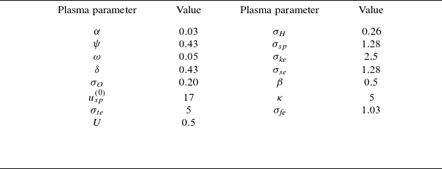
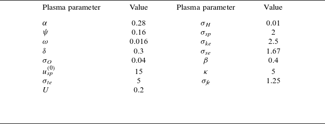
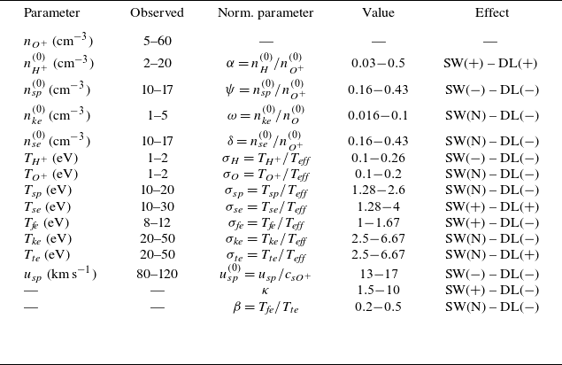
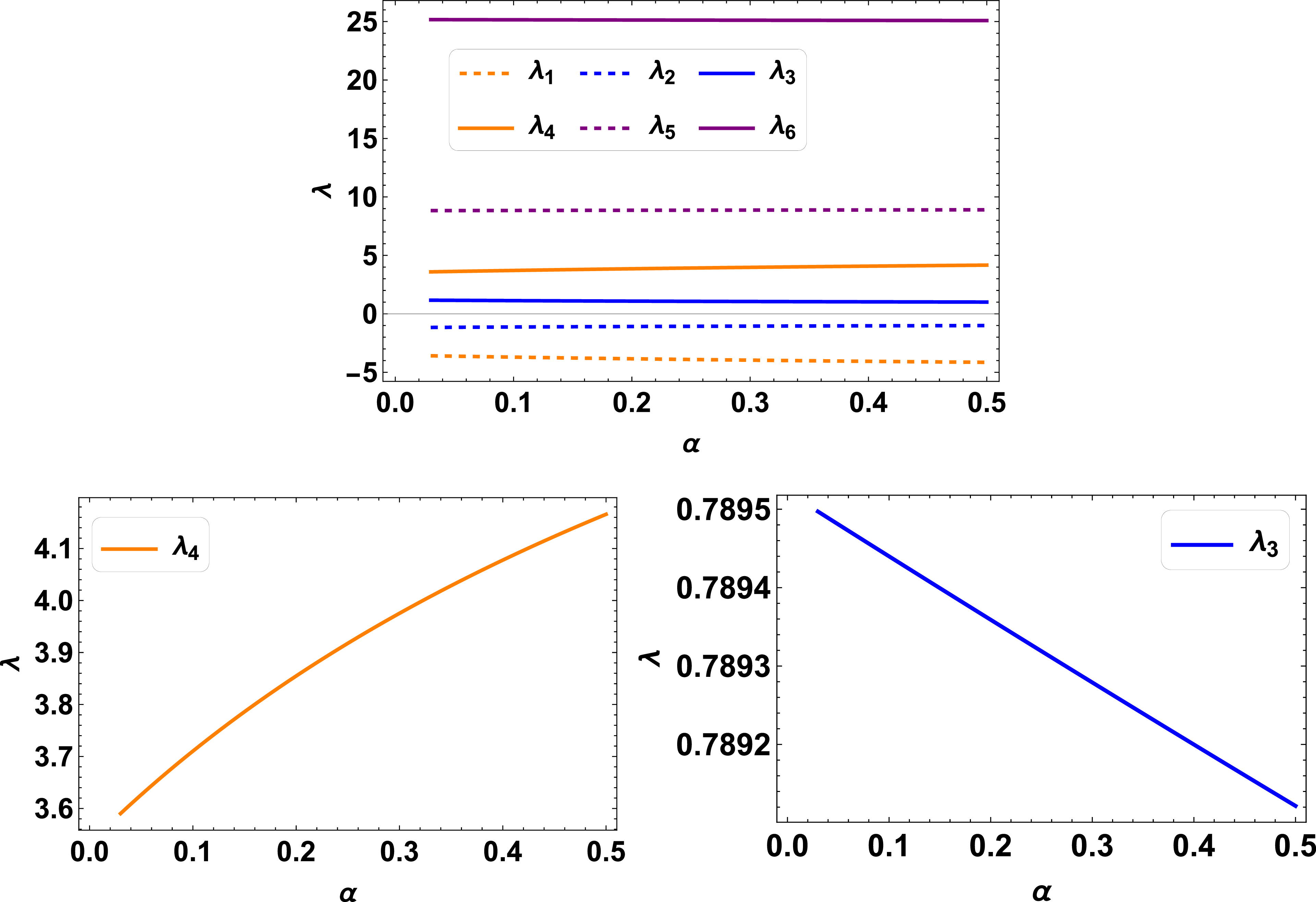


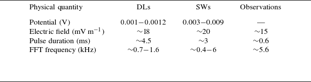

 Open access

