





1. Introduction
The transport of solutes with the flow of couple-stress fluid is highly relevant to micro- and nano-fluidic applications, as the couple-stress fluids, which mimic the rheology of several biofluids, can support couple stresses and body couples within the microstructure of the fluid (Stokes Reference Stokes1984). This model is particularly useful for describing the behaviour of fluids with internal structures or suspended particles, having important implications in biomedical contexts (Chaturani & Upadhya Reference Chaturani and Upadhya1978; Rudraiah, Pal & Siddheshwar Reference Rudraiah, Pal and Siddheshwar1986) and industrial processes (Ramanaiah & Sarkar Reference Ramanaiah and Sarkar1978). While several classical studies have explored electrokinetically actuated transport through microchannels and reported beneficial aspects of this flow actuation parameter in biomedical and industrial applications (Garcia et al. Reference Garcia, Ista, Petsev, O’brien, Bisong, Mammoli, Brueck and López2005; Li Reference Li2005; Tripathi, Bozkurt & Chauhan Reference Tripathi, Bozkurt and Chauhan2005; Masliyah & Bhattacherjee Reference Masliyah and Bhattacharjee2006; Ren & Stein Reference Ren and Stein2008; Schoch, Han & Renaud Reference Schoch, Han and Renaud2008; Ding, Jian & Tan Reference Ding, Jian and Tan2019; Ding & Jian Reference Ding and Jian2021; Ghosal Reference Ghosal2002a ,Reference Ghosal b ,Reference Ghosal c ; Alessio et al. Reference Alessio, Shim, Gupta and Stone2022), most of these works have focused primarily on electrohydrodynamics of Newtonian fluids and provided valuable insights into the underlying transport phenomenon. When the working fluid exhibits couple-stress behaviour, the underlying flow scenario driven by the combined influences of applied pressure gradients and electric field becomes more intricate, as microstructural interactions and intrinsic length scales significantly influence the velocity field. Moreover, much of the prior research has centred on transverse concentration profiles, with limited attention paid to the longitudinal variation rate of solute distribution – a critical aspect that remains unaddressed to date. The wall reactions, which are common in reactive solute transport processes, further highlight the behaviour of solute in electrokinetic transport (Reshadi & Saidi Reference Reshadi and Saidi2019; Sadeghi et al. Reference Sadeghi, Saidi, Moosavi and Sadeghi2020). The seminal works of Taylor (Reference Taylor1953) and Aris (Reference Aris1956) on solute transport phenomena in laminar tube flow provide foundational information into the enhanced mixing and spreading of solutes due to the interaction between molecular diffusion and flow velocity. The fundamental principles of hydrodynamic dispersion involve advection, diffusion and reaction mechanisms, which are often coupled and influenced by fluid properties and system geometry. In microfluidic systems, the reduced scale and high surface-to-volume ratio introduce unique challenges, such as enhanced surface interactions and non-uniform flow behaviours (Gervais & Jensen Reference Gervais and Jensen2006).
Further advancements in modelling solute dispersion have been achieved through multiscale analysis, which bridges the gap between microscopic (molecular) and macroscopic (continuum) scales. Multiscale approaches, such as homogenisation techniques and asymptotic analysis, enable the incorporation of detailed microstructural effects into macroscopic transport equations (Mei, Auriault & Ng Reference Mei, Auriault and Ng1996; Mei & Vernescu 2010). These methods provide a more accurate representation of solute dispersion by capturing the influence of microscopic heterogeneities, such as pore-scale variations and channel roughness, on overall transport behaviour (Hornung Reference Hornung1997; Bensoussan, Lions & Papanicolaou Reference Bensoussan, Lions and Papanicolaou2011). This multiscale framework is particularly useful in microfluidic applications, where intricate microscale interactions significantly impact macroscopic solute distribution and reaction rates. Several researchers have used this technique to study the effects of various key factors on solute dispersion in various flow and fluidic configurations (Wu, Li & Chen Reference Wu, Li and Chen2011; Wu & Chen Reference Wu and Chen2014; Dentz & de Barros Reference Dentz and de Barros2015; Barik & Dalal Reference Barik and Dalal2018; Aruna & Barik Reference Aruna and Barik2023; Chang & Santiago Reference Chang and Santiago2023; Das et al. Reference Das, Poddar, Dhar, Kairi and Mondal2021; Ding Reference Ding2023).
The combined pressure-driven and electro-osmotic effects lead to the development of complex velocity profiles, influencing solute transport and mixing. Moreover, the electric field can affect the movement and reaction of charged solutes, adding to the complexity of the system (Dejam Reference Dejam2019). Understanding these interactions is crucial for predicting and controlling solute transport in microchannels (Paul & Ng Reference Paul and Ng2012a ; Paul & Ng Reference Paul and Ng2012b ; Song, Ng & Law Reference Song, Ng and Law2014; Talebi, Ashrafizadeh & Sadeghi Reference Talebi, Ashrafizadeh and Sadeghi2021; Roy, Debnath & Bég Reference Roy, Debnath and Bég2023; Huang et al. Reference Huang, Debnath, Roy, Wang, Jiang, Bég and Kuharat2024; Das, Poddar & Kairi Reference Das, Poddar and Kairi2024). To this end, several studies have investigated solute dispersion phenomena following theoretical analysis, numerical simulations and explored the effect of pertinent parameters governing the underlying electrohydrodynamics on solute dispersion. Couple-stress fluids are a subclass of non-Newtonian fluids that contain microstructural elements which generate localised internal moments when subjected to deformation. These moments introduce higher-order stresses beyond classical viscous stresses. These stresses are accompanied by body couples, which together capture the influence of rotational interactions between neighbouring fluid elements (Stokes Reference Stokes1984). The foundational couple-stress theory was originally formulated by Stokes (Reference Stokes1984), who extended the classical continuum mechanics framework to include the influence of couple stresses. In this framework, the stress tensor is generalised to incorporate higher-order gradients of velocity, thereby capturing the rotational effects of the microstructures within the fluid. Such effects become particularly significant for the flow of biological fluids in microfluidic systems, where the microstructures induce complex rheological behaviour that departs markedly from Newtonian fluid assumptions. For example, blood flow in capillaries can be modelled accurately using couple-stress fluid dynamics (Valanis & Sun Reference Valanis and Sun1969; Pal, Rudraih & Devanathan Reference Pal, Rudraih and Devanathan1988; Funck, Laun & Wetscherek Reference Funck, Laun and Wetscherek2018; Chen, Lin & Chu Reference Chen, Lin and Chu2022). The transport of solutes in couple-stress fluids is influenced by the fluid’s microstructure and the associated couple stresses, which can alter the velocity profile (Pal et al. Reference Pal, Rudraih and Devanathan1988; Devakar & Iyenger Reference Devakar and Iyengar2010; Ahmed, Anwar Bég & Ghosh Reference Ahmed, Anwar Bég and Ghosh2014; Ishaq et al. Reference Ishaq, Rehman, Riaz and Zahid2024) and enhance mixing, thereby affecting the advection and diffusion of solutes. Additionally, couple stresses can influence solute–fluid interactions, further complicating transport dynamics (Soundalgekar Reference Soundalgekar1971; Almayehu & Radhakrishnamacharya Reference Alemayehu and Radhakrishnamacharya2010; Dhar, Mondal & Chadha Reference Dhar, Mondal and Chadha2024). While most previous works have focused mainly on the velocity behaviour of couple-stress fluids, relatively few have investigated solute dispersion in such systems. The present study aims to bridge this gap by exploring the impact of couple stress on solute transport in microchannels.
In many microfluidic systems, solute transport is significantly affected by chemical reactions, which may occur homogeneously within the bulk fluid or heterogeneously at the channel walls. Even in the case of irreversible reactions, such wall reactions can significantly influence the solute dispersion by depleting or modifying the concentration near the boundaries, thereby altering the effective transport dynamics. Due to the small dimensions and high surface-to-volume ratio, such reactions are often difficult to avoid, particularly in devices designed for biochemical sensing, catalytic processing or lab-on-a-chip applications (Demello Reference Demello2006; Ramon, Agnon & Dosoretz Reference Ramon, Agnon and Dosoretz2011; Sadeghi et al. Reference Sadeghi, Saidi, Moosavi and Sadeghi2020). Albeit several researchers have investigated the effect of wall reactions on solute dispersion in both Newtonian and non-Newtonian fluids flowing through parallel-plate channels or tubes (Wu et al. Reference Wu, Li and Chen2011; Wu & Chen Reference Wu and Chen2014; Barik & Dalal Reference Barik and Dalal2018; Jiang et al. Reference Jiang, Zeng, Fu and Wu2022; Aruna & Barik Reference Aruna and Barik2023; Das et al. 2023; Singh & Murthy Reference Singh and Murthy2023), very few studies have analytically examined this process in microchannel geometries (Gervais & Jensen Reference Gervais and Jensen2006; Ramon et al. Reference Ramon, Agnon and Dosoretz2011).
Over the past two decades, numerous research studies have built upon the work of Wu & Chen (Reference Wu and Chen2014), focusing extensively on the transverse variation rate of concentration distribution. The study by Das et al. (Reference Das, Poddar and Kairi2024) explored dispersion and mean concentration profiles in purely electro-osmotic flow (EOF) using a numerical approach. However, a complete analytical framework is still required to describe solute dispersion in couple-stress fluids under the combined influences of applied pressure gradients and imposed electrical field. This study fulfils the aforementioned need by providing an analytical solution to the two-dimensional convection–diffusion equation that takes into consideration boundary reactions and rheological behaviour in microfluidic systems. While classical Taylor dispersion theory captures longitudinal variations implicitly through an effective axial diffusivity, it does so by averaging over the cross-section and does not resolve the full axial concentration profile. However, our multiscale expansion yields an explicit analytical expression for this profile by going to the third order and enables a detailed examination of how key physical and rheological parameters influence longitudinal dispersion in couple-stress fluids, actuated by the combined effects of applied pressure gradients and electrical field. We define the longitudinal variation rate as a measure of how the concentration changes along the axial direction, evaluated at each transverse location. Specifically, it is computed as the difference between the maximum and minimum concentration values along the axial direction at a fixed transverse location, normalised by a reference concentration. We derive the unidirectional flow profile analytically by solving the Navier–Stokes equations in conjunction with interfacial electrostatics. We then solve the species transport equation using Mei’s multiscale homogenisation technique, considering the effects of couple-stress rheology and the chosen flow actuation parameter. We investigate the longitudinal variation rate of concentration and quantify how key parameters affect the underlying dispersion. Also, we discuss optimisation guidelines of microfluidic devices used in drug delivery, chemical sensing and other biotechnological fields. By addressing these objectives, this study contributes to the growing field of microfluidics and advances the fundamental understanding of solute transport in couple-stress fluids.
The remainder of the paper is organised as follows. Section 2 outlines the flow geometry and physical specifications of the problem, along with the assumptions. Section 3 presents the solution to the governing equations for the electrical double-layer (EDL) potential and axial velocity distribution. Additionally, the dispersion model for solute transport is described, and an analytical solution is derived using the multiple-scale homogenisation approach. Section 4 compares the analytical solution with numerical results and Brownian dynamics simulations, illustrated through graphical representations. Section 5 summarises the main findings of this study and discusses the impact of various parameters on the dispersion process, supported by graphical illustrations.
2. Flow and system set-up
We investigate the unsteady dispersion of a solute in a non-Newtonian couple-stress fluid, propelled by electro-osmotic effect in a long microchannel. We assume that the physical properties of the fluid are constant. We show in figure 1 the schematic depiction of the problem, including dimensions. The coordinate system is attached at the middle centre of the channel. We consider that the length of the microchannel is significantly higher than its height and width ( $2H\lt W\ll L$
). The length of the channel is taken along the
$2H\lt W\ll L$
). The length of the channel is taken along the $x^*$
direction, while the height and width of the channel are taken along the
$x^*$
direction, while the height and width of the channel are taken along the $y^*$
and
$y^*$
and $z^*$
directions, respectively. The flow is assumed to be steady and fully developed with possible solute absorption at the channel walls, modelled using an irreversible first-order boundary reaction. In addition to the electro-osmotic effect, we consider an applied pressure gradient along the
$z^*$
directions, respectively. The flow is assumed to be steady and fully developed with possible solute absorption at the channel walls, modelled using an irreversible first-order boundary reaction. In addition to the electro-osmotic effect, we consider an applied pressure gradient along the $ x^*$
direction to make the flow occur. The microchannel walls possess a net charge as represented by surface potential
$ x^*$
direction to make the flow occur. The microchannel walls possess a net charge as represented by surface potential $\zeta _{\alpha }^*$
. We assume that the surface potential is dependent on interfacial hydrodynamic slip.
$\zeta _{\alpha }^*$
. We assume that the surface potential is dependent on interfacial hydrodynamic slip.
We assume that, at $t^*=0.0$
, the dispersion begins with the instantaneous injection of a small amount of solute, uniformly distributed across the cross-section at
$t^*=0.0$
, the dispersion begins with the instantaneous injection of a small amount of solute, uniformly distributed across the cross-section at $x^*=0.0$
. This solute is subsequently transported by the combined electro-osmotic and pressure-driven flow (PDF) in the microchannel. The presence of couple-stress fluid, along with heterogeneous and homogeneous reactions, significantly affects the underlying dispersion process.
$x^*=0.0$
. This solute is subsequently transported by the combined electro-osmotic and pressure-driven flow (PDF) in the microchannel. The presence of couple-stress fluid, along with heterogeneous and homogeneous reactions, significantly affects the underlying dispersion process.
Schematic diagram describing the flow configuration considered in the present analysis. The height of the fluidic channel and the coordinate system are also shown in the schematic diagram.

3. Assessment of electric potential, flow dynamics and solute concentration
The basic equations describing the flow velocity and solute concentration are derived from the principle of mass conservation, momentum and the unsteady convection–diffusion equations. Pertaining to the symmetric electrolyte solution, the continuity, momentum and species transport equations for the present analysis can be written as follows:
 \begin{align}&\qquad\qquad\qquad {\boldsymbol{\nabla }\boldsymbol{\cdot }\boldsymbol {U}}=0, \end{align}
 \begin{align}& \rho \frac {D \boldsymbol {U}}{Dt^*}=-\boldsymbol{\nabla }P+ \mu {\nabla} ^2 \boldsymbol {U}-\eta {\nabla} ^4 \boldsymbol {U}+ \boldsymbol {F}_{\!d}, \end{align}
 \begin{align}& \frac {\partial C^*}{ \partial t^*}+{ \boldsymbol{\nabla }\boldsymbol{\cdot }(\boldsymbol {U} C^*)}=\boldsymbol{\nabla }(D \boldsymbol{\nabla }C^*){-K^*_1 C^*}{ .} \end{align}
Here, $\boldsymbol {U}$
,
$\boldsymbol {U}$
, $\mu$
,
$\mu$
, $\rho$
and
$\rho$
and $\eta$
represent the velocity, viscosity, density and couple-stress viscosity, respectively. The variable
$\eta$
represent the velocity, viscosity, density and couple-stress viscosity, respectively. The variable $t^*$
denotes time,
$t^*$
denotes time, $P$
is the time-independent pressure gradient,
$P$
is the time-independent pressure gradient, $K^*_1$
is the first-order bulk/body reaction,
$K^*_1$
is the first-order bulk/body reaction, $D$
is the molecular diffusivity, and
$D$
is the molecular diffusivity, and $C^*$
is the solute concentration. The electric body force
$C^*$
is the solute concentration. The electric body force $\boldsymbol {F}_{\!d}$
due to the EDL phenomenon is defined as
$\boldsymbol {F}_{\!d}$
due to the EDL phenomenon is defined as $\boldsymbol {F}_{\!d} = \rho _e\boldsymbol {E}$
, where
$\boldsymbol {F}_{\!d} = \rho _e\boldsymbol {E}$
, where $\boldsymbol {E}=(E_x,0,0)$
represents the electric field, and
$\boldsymbol {E}=(E_x,0,0)$
represents the electric field, and $\rho_e$
represents the net charge density.
$\rho_e$
represents the net charge density.
3.1. Electrical potential field
In this study, a symmetric electrolyte is assumed, wherein both ionic species possess equal but opposite valency (e.g. $\rm NaCl$
). This simplification allows analytical tractability of electrohydrodynamic equations, i.e. the Poisson–Nernst–Planck and momentum transport equations, and captures the essential features of electrokinetic transport in many practical settings. In addition, common electrolytes used in physiological and microfluidic systems, such as
$\rm NaCl$
). This simplification allows analytical tractability of electrohydrodynamic equations, i.e. the Poisson–Nernst–Planck and momentum transport equations, and captures the essential features of electrokinetic transport in many practical settings. In addition, common electrolytes used in physiological and microfluidic systems, such as $\rm NaCl$
and
$\rm NaCl$
and $\rm KCl$
, are typically symmetric in valency, which lends practical relevance to this assumption. Importantly, the focus of this work is to investigate solute dispersion in a couple-stress fluid under the influence of an electric field. Introducing ionic asymmetry would significantly increase the complexity of the model without altering the primary physical mechanisms under investigation. However, the symmetric electrolyte model has limitations, particularly when dealing with systems containing multivalent ions or strong ionic correlations. Recent work by Ding (Reference Ding2023) has shown that ionic asymmetry can lead to significant deviations in the structure of the electric double layer and the resulting EOF profiles.
$\rm KCl$
, are typically symmetric in valency, which lends practical relevance to this assumption. Importantly, the focus of this work is to investigate solute dispersion in a couple-stress fluid under the influence of an electric field. Introducing ionic asymmetry would significantly increase the complexity of the model without altering the primary physical mechanisms under investigation. However, the symmetric electrolyte model has limitations, particularly when dealing with systems containing multivalent ions or strong ionic correlations. Recent work by Ding (Reference Ding2023) has shown that ionic asymmetry can lead to significant deviations in the structure of the electric double layer and the resulting EOF profiles.
The Poisson equation is used to describe the induced electric field in the EDL as follows:
 \begin{equation} \frac {{\rm d}^2 \psi ^*}{{{\rm d}y^*}^2}=-\frac {\rho _e}{\delta }, \end{equation}
where $\psi ^*$
denotes the electric potential, and
$\psi ^*$
denotes the electric potential, and $\delta$
represents the dielectric constant of the electrolyte solution.
$\delta$
represents the dielectric constant of the electrolyte solution.
The ionic charge density can be expressed using the Boltzmann distribution, which for a symmetric electrolyte is given as $\rho _e=-2n_0 z_0 e \sinh ({z_0e\psi ^*}/({k_B T_{ab}}))$
, where
$\rho _e=-2n_0 z_0 e \sinh ({z_0e\psi ^*}/({k_B T_{ab}}))$
, where $n_0$
is the concentration of ions at the bulk,
$n_0$
is the concentration of ions at the bulk, $e$
is the charge of a proton,
$e$
is the charge of a proton, $k_B$
is Boltzmann’s constant,
$k_B$
is Boltzmann’s constant, $z_0$
is valence of the ions in the solution, and
$z_0$
is valence of the ions in the solution, and $T_{ab}$
is the average absolute temperature of the electrolytic solution.
$T_{ab}$
is the average absolute temperature of the electrolytic solution.
We appeal to the Debye–Hückel approximation (at low zeta potentials, typically less than $25\,\rm mV$
,
$25\,\rm mV$
, $\sinh ({z_0e\psi ^*}/({k_B T_{av}} ))$ $\thickapprox$ $({z_0e\psi ^*}/({k_B T_{av}} ))$
) to reduce (3.4) to the following form:
$({z_0e\psi ^*}/({k_B T_{av}} ))$
) to reduce (3.4) to the following form:
 \begin{equation} \frac {{\rm d}^2 \psi ^*}{{{\rm d} y^*}^2}=\kappa ^*{^2}\, \psi ^*, \end{equation}
where $\kappa ^*= ({2\,n_0 e^2 z_0^2}/({\delta \,k_B\,T_{ab}} ))^{1/2}$
.
$\kappa ^*= ({2\,n_0 e^2 z_0^2}/({\delta \,k_B\,T_{ab}} ))^{1/2}$
.
We consider the following expression of slip-dependent zeta potential in the present analysis (Soong, Hwang & Wang Reference Soong, Hwang and Wang2010; Banerjee et al Reference Banerjee, Mehta, Pati and Biswas2021):
 \begin{equation} \zeta ^*_\alpha =\zeta ^*\left [1+\alpha ^* \kappa ^*\right ]\!. \end{equation}
In this context, $\zeta ^*$
refers to the slip-independent (SI) zeta potential, whereas
$\zeta ^*$
refers to the slip-independent (SI) zeta potential, whereas $\zeta ^*_\alpha$
refers to the slip-dependent (SD) zeta potential. Furthermore,
$\zeta ^*_\alpha$
refers to the slip-dependent (SD) zeta potential. Furthermore, $\alpha ^*$
represents the slip length, and
$\alpha ^*$
represents the slip length, and $\kappa ^*$
denotes the dimensional Debye–Hückel parameter.
$\kappa ^*$
denotes the dimensional Debye–Hückel parameter.
We introduce the following dimensionless quantities to cast (3.5) and (3.6) in their dimensionless counterparts:
 \begin{equation} y=\frac {y^*}{H}, \psi =\frac {\psi ^*}{\psi _r}, \kappa =\kappa ^* H, \psi _r=\frac {k_B T_{ab}}{e z_0}, \alpha =\frac {\alpha ^*}{H}, \end{equation}
where, $\kappa$
and
$\kappa$
and $\alpha$
represent dimensionless quantities, with
$\alpha$
represent dimensionless quantities, with $\kappa$
being the Debye–Hückel parameter and
$\kappa$
being the Debye–Hückel parameter and $\alpha$
denoting the slip length.
$\alpha$
denoting the slip length.
The dimensionless forms of (3.5) and (3.6) are written as
 \begin{equation} \frac {{\rm d}^2 \psi }{{{\rm d} y}^2}=\kappa ^2\, \psi \end{equation}
and
 \begin{equation} \zeta _\alpha =\zeta \left [1+\alpha \kappa \right ]\!, \end{equation}
where $\zeta$
is the dimensionless slip-independent (SI) zeta potential. The following dimensionless boundary conditions are employed to calculate the EDL potential, influenced by the interfacial slip:
$\zeta$
is the dimensionless slip-independent (SI) zeta potential. The following dimensionless boundary conditions are employed to calculate the EDL potential, influenced by the interfacial slip:
 \begin{equation} \psi =\zeta _\alpha \quad \mbox{at} \quad y=\pm 1. \end{equation}
We write the expression of the dimensionless EDL potential as
 \begin{equation} \psi (y)=\zeta _\alpha \frac {\cosh (\kappa y)}{\cosh (\kappa )}. \end{equation}
3.2. Velocity distribution
A couple-stress fluid is a non-Newtonian fluid characterised by internal strains arising from microrotations or suspended particles. These stresses are represented by a second-order couple-stress tensor, which extends the conventional stress tensor to account for body couples and rotational effects. The present work utilises the couple-stress fluid model as outlined in the studies by Stokes (Reference Stokes1984), Devakar & Iyenger (Reference Devakar and Iyengar2010) and Siva et al. (Reference Siva, Kumbhakar, Jangili and Mondal2020).
The present analysis is based on the assumption of a unidirectional flow field, such that the leading-order velocity takes the form $\boldsymbol{U} = (u^*(y^*), 0, 0)$
, without dependence on the axial coordinate
$\boldsymbol{U} = (u^*(y^*), 0, 0)$
, without dependence on the axial coordinate $ x^*$
. This simplification is valid for slender geometries (
$ x^*$
. This simplification is valid for slender geometries ( $2H \ll W$
) and low-Reynolds-number flows, where inertial effects are negligible. Under this assumption, the velocity gradients in the axial direction vanish, i.e.
$2H \ll W$
) and low-Reynolds-number flows, where inertial effects are negligible. Under this assumption, the velocity gradients in the axial direction vanish, i.e. $\partial u^* / \partial x^* = 0$
, and the inertial terms are omitted from the momentum equations. However, it is worth mentioning here that the longitudinal variations in the flow field, where
$\partial u^* / \partial x^* = 0$
, and the inertial terms are omitted from the momentum equations. However, it is worth mentioning here that the longitudinal variations in the flow field, where $\boldsymbol{U} = \boldsymbol{U}(x^*, y^*, z^*)$
, can arise in more general settings, such as in the presence of spatial heterogeneities, unsteady forcing or varying channel geometry. Considering the assumption made in this analysis, the equation governing the underlying transport can be written as
$\boldsymbol{U} = \boldsymbol{U}(x^*, y^*, z^*)$
, can arise in more general settings, such as in the presence of spatial heterogeneities, unsteady forcing or varying channel geometry. Considering the assumption made in this analysis, the equation governing the underlying transport can be written as
 \begin{eqnarray} && -\frac {{\rm d}p}{{\rm d}x^*}+\mu \frac {{\rm d}^2u^*}{{{\rm d}y^*}^2}-\eta \frac {{\rm d}^4u^*}{{{\rm d}y^*}^4}+\rho _e E_x=0, \end{eqnarray}
where $p$
is the pressure. Using (3.4), (3.12) reduces to
$p$
is the pressure. Using (3.4), (3.12) reduces to
 \begin{eqnarray} && -\frac {{\rm d}p}{{\rm d}x^*}+\mu \frac {{\rm d}^2u^*}{{{\rm d}y^*}^2}-\eta \frac {{\rm d}^4u^*}{{{\rm d}y^*}^4}-\delta E_x\frac {{\rm d}^2\psi ^*}{{{\rm d}y^*}^2}=0. \end{eqnarray}
We employ in the endeavour slip boundary condition, consistent with the Navier-slip model described as follows:
 \begin{equation} u^*-\alpha ^*\frac {{\rm d} u^*}{{\rm d}y^*} \Bigg |_{\,y^*=-H}=u^*+\alpha ^*\frac {{\rm d} u^*}{{\rm d}y^*} \Bigg |_{\,y^*=H}=\frac {{\rm d}^2u^*}{{{\rm d}y^*}^2}\Bigg |_{\,y^*=\pm H}=0. \end{equation}
The pressure gradient that drives the flow can be represented as
 \begin{equation} \frac {{\rm d} p}{{\rm d} x^*}=G. \end{equation}
To write (3.13) in the dimensionless form in addition to the dimensionless quantities, we introduce a few parameters as follows:
 \begin{equation} u=\frac {u^*}{u_{\textit{HS}}}, \varGamma =\frac {GH^2}{ \mu u_{\textit{HS}}}, u_{\textit{HS}}=-\frac {\delta \psi _r E_x}{\mu }, B=\sqrt {\frac {\mu H^2}{\eta }}, \end{equation}
where $\varGamma$
is the forcing comparison parameter,
$\varGamma$
is the forcing comparison parameter, $u_{\textit{HS}}$
is the Helmholtz–Smoluchowski velocity, and
$u_{\textit{HS}}$
is the Helmholtz–Smoluchowski velocity, and $B$
is the couple-stress parameter.
$B$
is the couple-stress parameter.
Using (3.16), the dimensionless from of (3.13) is given by
 \begin{equation} \frac {{\rm d}^2u}{{\rm d}y^2}-\frac {1}{B^2}\frac {{\rm d}^4u}{{\rm d}y^4}=\frac {GH^2}{ \mu u_{\textit{HS}}}- \zeta _\alpha \kappa ^2\frac {\cosh (\kappa y)}{\cosh (\kappa )}. \end{equation}
The dimensionless form of the boundary condition of (3.14) is given as
 \begin{equation} u-\alpha \frac {{\rm d} u}{{\rm d}y} \Bigg |_{\,y=-1}=u+\alpha \frac {{\rm d} u}{{\rm d}y} \Bigg |_{\,y=1}=\frac {{\rm d}^2u}{{{\rm d}y}^2}\Bigg |_{\,y=\pm 1}=0. \end{equation}
Using the conditions (3.18) in (3.17), the dimensionless velocity profile is found as
 \begin{equation} u(y)=\frac {\varGamma }{B^2}\left (1-\frac {\cosh B y}{\cosh B}\right )+\frac { \zeta _\alpha }{\kappa ^2-B^2}\left (B^2\frac {\cosh \kappa y}{\cosh \kappa }-\kappa ^2\frac {\cosh B y}{\cosh B}\right )-\left(C_1-\varGamma \frac {y^2}{2}\right)\!, \end{equation}
where, $C_1={(\zeta _\alpha B^2}/{(\kappa ^2-B^2))} (1+\alpha \kappa \tanh \kappa )-({1}/{\cosh B}) (({\varGamma }/{B^2})+({(\zeta _\alpha \kappa ^2)}/ {(\kappa ^2-B^2)} ) (\cosh B+\alpha B \sinh B )+\varGamma (({1}/{B^2})+\alpha +({1}/{2})).$
3.3. Homogenisation of concentration
The unsteady transport of solute, driven by solvent flow and molecular diffusion, is described by (3.3). At time $t^*=0.0$
, a solute of known concentration, distributed uniformly across the cross-section, is released instantaneously at the inlet. The solute concentration distribution
$t^*=0.0$
, a solute of known concentration, distributed uniformly across the cross-section, is released instantaneously at the inlet. The solute concentration distribution $C^*(x^*, y^*, t^*)$
in the channel is governed by the following equation:
$C^*(x^*, y^*, t^*)$
in the channel is governed by the following equation:
 \begin{equation} \frac {\partial C^*}{ \partial t^*}+u^*\frac {\partial C^*}{\partial x^* }=D\left (\frac {\partial ^2C^*}{\partial {x^*}^2}+\frac {\partial ^2 C^*}{\partial {y^*}^2}\right )-K_1^*C^*,\quad -H\lt y^*\lt H. \end{equation}
We use the following initial and boundary conditions to solve (3.20):
 \begin{align}& \left .C^* \big(x^*, y^*, t^* \big)\right |_{t^*=0}=C^0\delta \left (\frac {x^*}{H}\right )\!, \end{align}
 \begin{align}&\quad\, \left [D\frac {\partial C^*}{\partial y^*}+\beta _1^{*} C^*\right ]_{y^*= H}=0, \end{align}
 \begin{align}&\quad \left [D\frac {\partial C^*}{\partial y^*}-\beta _2^{*} C^*\right ]_{y^*= -H}=0, \end{align}
 \begin{align}&\quad C^* \big(x^*,y^*,t^* \big)|_{x^*\rightarrow \pm \infty }=0{,} \end{align}
where $\delta (.)$
the Dirac delta function,
$\delta (.)$
the Dirac delta function, $\beta^*_1$
and
$\beta^*_1$
and $\beta^*_2$
are the dimensional boundary absorption at the upper and lower walls of the channel, and
$\beta^*_2$
are the dimensional boundary absorption at the upper and lower walls of the channel, and $C^0$
is the reference concentration.
$C^0$
is the reference concentration.
3.3.1. Dimensionless governing equation
The dimensionless parameters are introduced accordingly
 \begin{equation} x=\frac {x^*}{L}, C=\frac {C^*}{C^0}, t=\frac {t^*}{H^2/D}, \beta ^{\prime}_1=\frac {\beta _1^{*} L}{D}, \beta ^{\prime}_2=\frac {\beta _2^{*} L}{D}, K^{\prime}_1=\frac {K_1^* L^2}{D}. \end{equation}
The dimensionless solute transport equation reads as
 \begin{equation} \frac {\partial C}{ \partial t}+\varepsilon u \textit{Pe}\frac {\partial C}{\partial x}=\varepsilon ^2\frac {\partial ^2C}{\partial {x}^2}+\frac {\partial ^2 C}{\partial {y}^2}-\varepsilon ^2K^{\prime}_1C,\quad -1\lt y\lt 1. \end{equation}
We write the corresponding boundary conditions as
 \begin{align} \left [\frac {\partial C}{\partial y}+\varepsilon \beta ^{\prime}_1 C\right ]_{y= 1}&=0, \end{align}
 \begin{align} \left [\frac {\partial C}{\partial y}-\varepsilon \beta ^{\prime}_2 C\right ]_{y=-1}&=0, \end{align}
where $\varepsilon ={H}/{L}(\ll 1)$
is the perturbation parameter, and
$\varepsilon ={H}/{L}(\ll 1)$
is the perturbation parameter, and ${\textit{Pe}}={u_{\textit{HS}} H}/{D}$
is the diffusive Péclet number, which is defined as the ratio of the convection rate
${\textit{Pe}}={u_{\textit{HS}} H}/{D}$
is the diffusive Péclet number, which is defined as the ratio of the convection rate $ ({1}/{(H/u_{\textit{HS}})})$
to the diffusion rate
$ ({1}/{(H/u_{\textit{HS}})})$
to the diffusion rate $ ({1}/({H^2/D})$
. The Péclet number is taken to be of order unity (
$ ({1}/({H^2/D})$
. The Péclet number is taken to be of order unity ( ${\textit{Pe}} = \mathcal{O}(1)$
) (Mei et al. Reference Mei, Auriault and Ng1996).
${\textit{Pe}} = \mathcal{O}(1)$
) (Mei et al. Reference Mei, Auriault and Ng1996).
3.3.2. Homogenisation
For the present study, we used the multiscale homogenisation method (Mei et al. Reference Mei, Auriault and Ng1996; Mei & Vernescu 2010). The method adopts three different time scales: $T_0={H^2}/{D}$
represents the diffusion time across the channel height,
$T_0={H^2}/{D}$
represents the diffusion time across the channel height, $T_1={L}/{u_{\textit{HS}}}$
represents the convection time across the characteristic length of the microchannel, and
$T_1={L}/{u_{\textit{HS}}}$
represents the convection time across the characteristic length of the microchannel, and $T_2={L^2}/{D}$
represents the diffusion time across the channel length. The ratio of these three time scales is
$T_2={L^2}/{D}$
represents the diffusion time across the channel length. The ratio of these three time scales is
 \begin{equation} T_0:T_1:T_2=1:\frac {1}{\varepsilon }:\frac {1}{\varepsilon ^2}. \end{equation}
We consider the following three time variables, which are inversely proportional to the time scales reported by Mei et al. (Reference Mei, Auriault and Ng1996), corresponding to fast, medium and slow time scales:
 \begin{equation} t_0=t, t_1=\varepsilon t, t_2=\varepsilon ^2t. \end{equation}
Using the chain rule, one can get the original time derivative:
 \begin{equation} \frac {\partial }{\partial t}=\frac {\partial }{\partial t_0}+\varepsilon \frac {\partial }{\partial t_1}+\varepsilon ^2\frac {\partial }{\partial t_2}. \end{equation}
The asymptotic expression of solute concentration $C$
can be expanded into multiscale and given as (Fife & Nicholes Reference Fife and Nicholes1975)
$C$
can be expanded into multiscale and given as (Fife & Nicholes Reference Fife and Nicholes1975)
 \begin{align} C(x,y,t) &=C_0(x,y,t_0,t_1,t_2)+\varepsilon C_1(x,y,t_0,t_1,t_2)+\varepsilon ^2 C_2(x,y,t_0,t_1,t_2)\nonumber \\ &\quad+\varepsilon ^3 C_3(x,y,t_0,t_1,t_2)+O(\varepsilon ^4), \end{align}
where $C_0, C_1, C_2$
and
$C_0, C_1, C_2$
and $C_3$
are the zeroth, first, second, and third order concentration of solute. Substituting (3.31) and (3.32) into (3.26)–(3.28) we get
$C_3$
are the zeroth, first, second, and third order concentration of solute. Substituting (3.31) and (3.32) into (3.26)–(3.28) we get
 \begin{align} &\left (\frac {\partial C_{0}}{\partial t_0}-\frac {\partial ^2 C_{0}}{\partial y^2}\right )+\varepsilon \left (\frac {\partial C_{0}}{\partial t_1}+\frac {\partial C_{1}}{\partial t_0}+uPe\frac {\partial C_{0}}{\partial x}-\frac {\partial ^2 C_{1}}{\partial y^2}\right )+\varepsilon ^2\left (\frac {\partial C_{0}}{\partial t_2}+\frac {\partial C_{1}}{\partial t_1}\right . \nonumber \\&\quad\left .+\frac {\partial C_{2}}{\partial t_0}+uPe\frac {\partial C_{1}}{\partial x}-\frac {\partial ^2 C_{0}}{\partial x^2}-\frac {\partial ^2 C_{2}}{\partial y^2}+K^{\prime}_1C_0\right )+\varepsilon ^3\left (\frac {\partial C_{1}}{\partial t_2}+\frac {\partial C_{2}}{\partial t_1}+\frac {\partial C_{3}}{\partial t_0}\right . \nonumber \\ &\quad \left .+uPe\frac {\partial C_{2}}{\partial x}-\frac {\partial ^2 C_{1}}{\partial x^2}-\frac {\partial ^2 C_{3}}{\partial y^2}+K^{\prime}_1C_1\right )+O(\varepsilon ^4)=0,\quad -1\lt y\lt 1& \end{align}
and
 \begin{align} &\frac {\partial C_{0}}{\partial y}+\varepsilon \left (\!\frac {\partial C_{1}}{\partial y}+\beta ^{\prime}_1 C_0\!\right )+\varepsilon ^2\left (\!\frac {\partial C_{2}}{\partial y}+\beta ^{\prime}_1 C_1\!\right )+\varepsilon ^3\left (\!\frac {\partial C_{3}}{\partial y}+\beta ^{\prime}_1 C_2\!\right )+O(\varepsilon ^4)=0 \mbox{ at }y=1,& \end{align}
 \begin{align} &\frac {\partial C_{0}}{\partial y}+\varepsilon \!\left (\!\frac {\partial C_{1}}{\partial y}-\beta ^{\prime}_2 C_0\!\right )+\varepsilon ^2\!\left (\!\frac {\partial C_{2}}{\partial y}-\beta ^{\prime}_2 C_1\!\right )+\varepsilon ^3\!\left (\!\frac {\partial C_{3}}{\partial y}-\beta ^{\prime}_2 C_2\!\right )+O(\varepsilon ^4)=0 \mbox{ at } y=-1. & \end{align}
3.3.3. Zeroth-order perturbation $(O(\varepsilon ^0))$

For the zeroth-order $(O(\varepsilon ^0))$
perturbation, (3.33) and boundary conditions (3.34)–(3.35) give
$(O(\varepsilon ^0))$
perturbation, (3.33) and boundary conditions (3.34)–(3.35) give
 \begin{equation} \frac {\partial C_{0}}{\partial t_0}=\frac {\partial ^2 C_{0}}{\partial y^2},\quad -1\lt y\lt 1 \end{equation}
and
 \begin{equation} \left .\frac {\partial C_{0}}{\partial y}\right |_{y=\pm 1}=0. \end{equation}
The general solution of (3.36), utilising the boundary conditions in (3.37), is given by
 \begin{equation} C_{0}=C_{0}^{(0)}(x,t_1,t_2) +\sum _{n=1}^{\infty }{Re}\left [C_0^{(n)}(x,t_1,t_2)e^{\textrm{i}n\unicode{x03C0} y}\right ]e^{-n^2\unicode{x03C0} ^2t_0}{.} \end{equation}
The series term is excluded because it rapidly diminishes over long-time evolution, and the solution of (3.38) becomes
 \begin{equation} C_0=C_0(x,t_1,t_2). \end{equation}
3.3.4. First-order perturbation
$(O(\varepsilon ^1))$

Since $C_0$
is independent of
$C_0$
is independent of $y$
also, we obtain the first-order
$y$
also, we obtain the first-order $(O(\varepsilon ^1))$
perturbation problem as follows:
$(O(\varepsilon ^1))$
perturbation problem as follows:
 \begin{equation} \frac {\partial C_{0}}{\partial t_1}+\frac {\partial C_{1}}{\partial t_0}+uPe\frac {\partial C_{0}}{\partial x}=\frac {\partial ^2 C_{1}}{\partial y^2} \end{equation}
and
 \begin{align}&\, \left [\frac {\partial C_{1}}{\partial y}+\beta ^{\prime}_1 C_0\right ]_{y=1}=0, \end{align}
 \begin{align}& \left [\frac {\partial C_{1}}{\partial y}-\beta ^{\prime}_2 C_0\right ]_{y=-1}=0. \end{align}
Following a standard long-time asymptotic approach, we consider $t_0 \gg 1$
while
$t_0 \gg 1$
while $t_1$
remains finite (Teng, Rallabandi & Ault Reference Teng, Rallabandi and Ault2023). Pertaining to this limiting condition, the derivative
$t_1$
remains finite (Teng, Rallabandi & Ault Reference Teng, Rallabandi and Ault2023). Pertaining to this limiting condition, the derivative ${\partial C_{1}}/({\partial t_0})$
becomes negligibly small and has been omitted from (3.40), which yields
${\partial C_{1}}/({\partial t_0})$
becomes negligibly small and has been omitted from (3.40), which yields
 \begin{equation} \frac {\partial C_{0}}{\partial t_1}+uPe\frac {\partial C_{0}}{\partial x}=\frac {\partial ^2 {C_{1}}}{\partial y^2}. \end{equation}
Further, the height average of a function $f$
is defined with respect to
$f$
is defined with respect to $y$
as
$y$
as
 \begin{equation} \left \langle f\right \rangle =\frac {1}{2}\int _{-1}^{1}f {\rm d} y. \end{equation}
The height-average expression of $C_0$
and
$C_0$
and ${\partial ^2 {C_n}}/({ \partial y^2})$
obtained using (3.44) take the form
${\partial ^2 {C_n}}/({ \partial y^2})$
obtained using (3.44) take the form $\langle C_0\rangle =C_0$
and
$\langle C_0\rangle =C_0$
and $\langle {\partial ^2 {C_n}}/({ \partial y^2})\rangle=-({1}/{2}) (\beta ^{\prime}_1 C_{n-1}|_{y=1}+\beta ^{\prime}_2 C_{n-1}|_{y=-1} )$
for
$\langle {\partial ^2 {C_n}}/({ \partial y^2})\rangle=-({1}/{2}) (\beta ^{\prime}_1 C_{n-1}|_{y=1}+\beta ^{\prime}_2 C_{n-1}|_{y=-1} )$
for $n=1,2,3.$
Next by taking the height-average form of (3.43) with respect to the spatial variable $y$
subject to the boundary conditions (3.41) and (3.42), we get
$y$
subject to the boundary conditions (3.41) and (3.42), we get
 \begin{equation} \frac {\partial C_{0}}{\partial t_1}+\left \langle u\right \rangle{\textit{Pe}}\frac {\partial C_{0}}{\partial x}=-\frac {1}{2}\left (\beta ^{\prime}_1+\beta ^{\prime}_2\right )C_0. \end{equation}
By subtracting (3.45) from (3.40), and noting that $C_0$
is independent of
$C_0$
is independent of $y$
, we obtain
$y$
, we obtain
 \begin{equation}{\textit{Pe}}\left (u-\left \langle u\right \rangle \right )\frac {\partial C_{0}}{\partial x}-\frac {1}{2}\left (\beta ^{\prime}_1+\beta ^{\prime}_2\right )C_0=\frac {\partial ^2 C_{1}}{\partial y^2}. \end{equation}
Equation (3.46) indicates the following substitution:
 \begin{equation} C_1=Pe A_1(y)\frac {\partial C_0}{\partial x}+\frac {1}{2}\left (\beta ^{\prime}_1+\beta ^{\prime}_2\right )A_2(y)C_0. \end{equation}
By comparing the terms adhered to $({\partial C_0}/({\partial x}))$
and
$({\partial C_0}/({\partial x}))$
and $C_0$
, we obtain the boundary-value problems for transverse functions
$C_0$
, we obtain the boundary-value problems for transverse functions $A_1(y)$
and
$A_1(y)$
and $A_2(y)$
, which are presented in Appendix A.
$A_2(y)$
, which are presented in Appendix A.
3.3.5. Second-order perturbation
$(O(\varepsilon ^2))$

For second-order $(O(\varepsilon ^2))$
perturbation, (3.33)–(3.35) give
$(O(\varepsilon ^2))$
perturbation, (3.33)–(3.35) give
 \begin{equation} \frac {\partial C_{0}}{\partial t_2}+\frac {\partial C_{1}}{\partial t_1}+\frac {\partial C_{2}}{\partial t_0}+uPe\frac {\partial C_{1}}{\partial x}=\frac {\partial ^2 C_{0}}{\partial x^2}+\frac {\partial ^2 C_{2}}{\partial y^2}-K^{\prime}_1C_0,\quad -1\lt y\lt 1 \end{equation}
and
 \begin{align}&\,\left [\frac {\partial C_{2}}{\partial y}+\beta ^{\prime}_1 C_1\right ]_{y= 1}=0, \end{align}
 \begin{align}& \left [\frac {\partial C_{2}}{\partial y}-\beta ^{\prime}_2 C_1\right ]_{y= -1}=0. \end{align}
Similarly, under the same long-time assumption $t_0 \gg 1$
, the term
$t_0 \gg 1$
, the term $({\partial C_{2}}/({\partial t_0}))$
becomes negligibly small. Eliminating this term from (3.48) simplifies it to the following:
$({\partial C_{2}}/({\partial t_0}))$
becomes negligibly small. Eliminating this term from (3.48) simplifies it to the following:
 \begin{equation} \frac {\partial C_{0}}{\partial t_2}+\frac {\partial {C_{1}}}{\partial t_1}+uPe{\frac {\partial C_{1}}{\partial x}}=\frac {\partial ^2 C_{0}}{\partial x^2}+\frac {\partial ^2 {C_{2}}}{\partial y^2}-K^{\prime}_1C_0. \end{equation}
Further, taking the section average of (3.51) with respect to spatial variable $y$
subject to the boundary conditions (3.49)–(3.50), we get
$y$
subject to the boundary conditions (3.49)–(3.50), we get
 \begin{equation} \frac {\partial C_{0}}{\partial t_2}+\frac {\partial \left \langle {C_{1}}\right \rangle }{\partial t_1}+Pe\left \langle {u\frac {\partial C_{1}}{\partial x}}\right \rangle =\frac {\partial ^2 C_{0}}{\partial x^2}-\frac {1}{2}\left [\beta ^{\prime}_1C_1(1)+\beta ^{\prime}_2C_1(-1)\right ]-K^{\prime}_1C_0. \end{equation}
Subtracting (3.52) from (3.48), one can get
 \begin{equation} \frac {\partial C_{2}}{\partial t_0}+\frac {\partial C_{1}}{\partial t_1}+Pe{u\frac {\partial C_{1}}{\partial x}}-{\textit{Pe}}\left \langle {u\frac {\partial C_{1}}{\partial x}}\right \rangle -\frac {\partial \left \langle {C_{1}}\right \rangle }{\partial t_1}=\frac {\partial ^2 C_{2}}{\partial y^2}+\frac {1}{2}\left [\beta ^{\prime}_1C_1(1)+\beta ^{\prime}_2C_1(-1)\right ]\!. \end{equation}
From (3.45) (3.47), (A3) and (3.19), the following terms of (3.53) can be found as
 \begin{align} &\qquad\qquad\qquad\qquad\qquad\qquad \frac {\partial \left \langle {C_{1}}\right \rangle }{\partial t_1}=0, \end{align}
 \begin{align} & \frac {\partial C_{1}}{\partial t_1}=-{\textit{Pe}}^2\left \langle u\right \rangle A_1\frac {\partial ^2 C_{0}}{\partial x^2}-\frac {\textit{Pe}}{2}\left (\beta ^{\prime}_1+\beta ^{\prime}_2\right )\left (A_1+\left \langle u\right \rangle A_2\right )\frac {\partial C_{0}}{\partial x}-\frac {1}{4}\left (\beta ^{\prime}_1+\beta ^{\prime}_2\right )^2A_2C_0, \end{align}
 \begin{align} &\qquad\qquad\qquad {u\frac {\partial C_{1}}{\partial x}}=Pe\,uA_1\frac {\partial ^2 C_{0}}{\partial x^2}+\frac {1}{2}\left (\beta ^{\prime}_1+\beta ^{\prime}_2\right )uA_2\frac {\partial C_{0}}{\partial x}, \end{align}
 \begin{align} &\qquad\qquad \left \langle {u\frac {\partial C_{1}}{\partial x}}\right \rangle =Pe\left \langle uA_1\right \rangle \frac {\partial ^2 C_{0}}{\partial x^2}+\frac {1}{2}\left (\beta ^{\prime}_1+\beta ^{\prime}_2\right )\left \langle uA_2\right \rangle \frac {\partial C_{0}}{\partial x}. \end{align}
Substituting (3.54)–(3.57) in (3.53), one can get
 \begin{align} \frac {\partial C_{2}}{\partial t_0}&+ {\textit{Pe}}^2\left [uA_1-\left \langle u\right \rangle A_1-\left \langle uA_1\right \rangle \right ]\frac {\partial ^2 C_{0}}{\partial x^2}\nonumber\\& +\frac {\textit{Pe}}{2}\left(\beta ^{\prime}_1+\beta ^{\prime}_2\right)\left [uA_2-\left \langle uA_2\right \rangle -A_1-\left \langle u\right \rangle A_2-\frac {\beta ^{\prime}_1A_1(1)+\beta ^{\prime}_2A_1(-1)}{\beta ^{\prime}_1+\beta ^{\prime}_2}\right ]\frac {\partial C_{0}}{\partial x}\nonumber\\& -\frac {1}{4}(\beta ^{\prime}_1+\beta ^{\prime}_2)^2\left \{A_2+\frac {\beta ^{\prime}_1 A_2(1)+\beta ^{\prime}_2A_2(-1)}{\beta ^{\prime}_1+\beta ^{\prime}_2}\right \}C_0=\frac {\partial ^2 C_{2}}{\partial y^2}. \end{align}
Equation (3.58) indicates the following substitution:
 \begin{equation} C_2={\textit{Pe}}^2A_3(y)\frac {\partial ^2 C_{0}}{\partial x^2}+\frac {\textit{Pe}}{2}\big(\beta ^{\prime}_1+\beta ^{\prime}_2 \big)A_4(y)\frac {\partial C_{0}}{\partial x}+\frac {1}{4} \big(\beta ^{\prime}_1+\beta ^{\prime}_2 \big)^2A_5(y)C_0. \end{equation}
On comparing the terms associated with $({\partial ^2 C_{0}}/({\partial x^2}))$
,
$({\partial ^2 C_{0}}/({\partial x^2}))$
, $({\partial C_{0}}/({\partial x}))$
and
$({\partial C_{0}}/({\partial x}))$
and $C_0$
, we obtain the boundary-value problems for transverse functions
$C_0$
, we obtain the boundary-value problems for transverse functions $A_3(y)$
,
$A_3(y)$
, $A_4(y)$
and
$A_4(y)$
and $A_5(y)$
, which are presented in Appendix B.
$A_5(y)$
, which are presented in Appendix B.
Note that the intermediate mathematical steps and the boundary-value problem corresponding to the third-order perturbation $(O(\varepsilon ^3))$
are provided in Appendix C.
$(O(\varepsilon ^3))$
are provided in Appendix C.
3.3.6. Taylor dispersion coefficient
Substituting (3.54), (3.57) in (3.52), we get
 \begin{align} \frac {\partial C_{0}}{\partial t_2}+\frac {\textit{Pe}}{2}\left (\beta ^{\prime}_1+\beta ^{\prime}_2\right )\left \langle uA_2\right \rangle \frac {\partial C_{0}}{\partial x}& = \big(1-{\textit{Pe}}^2\left \langle uA_1\right \rangle \big)\frac {\partial ^2 C_{0}}{\partial x^2}-\frac {1}{2}\left [\beta ^{\prime}_1C_1(1)+\beta ^{\prime}_2C_1(-1)\right ]\nonumber\\&\quad -K^{\prime}_1C_0. \end{align}
Multiplying (3.45) by $\varepsilon$
and (3.60) by
$\varepsilon$
and (3.60) by $\varepsilon ^2$
and adding them together, we get
$\varepsilon ^2$
and adding them together, we get
 \begin{align} &\frac {\partial C_0}{\partial t_0}+\varepsilon \frac {\partial C_0}{\partial t_1}+\varepsilon ^2\frac {\partial C_0}{\partial t_2}+\varepsilon \textit{Pe}\!\left [\!\left \langle u\right \rangle +\frac {\varepsilon }{2} \big(\beta ^{\prime}_1+\beta ^{\prime}_2 \big)\left \langle uA_2\right \rangle +\frac {\varepsilon }{2}\beta ^{\prime}_1A_1(1)+\frac {\varepsilon }{2}\beta ^{\prime}_2A_1(-1)\!\right ]\frac {\partial C_0}{\partial x} \nonumber\\ &=\varepsilon ^2\left [1-{\textit{Pe}}^2\left \langle uA_1\right \rangle \right ]\frac {\partial ^2 C_0}{\partial x^2}\nonumber \\ &\quad -\left [\frac {\varepsilon }{2} \big(\beta ^{\prime}_1+\beta ^{\prime}_2 \big)+\frac {\varepsilon ^2}{4} \big(\beta ^{\prime}_1+\beta ^{\prime}_2 \big)\left \{\beta ^{\prime}_1A_2(1)+\beta ^{\prime}_2A_2(-1)\right \}+\varepsilon ^2K^{\prime}_1\right ]C_0. \end{align}
In terms of original time variable $t$
, (3.61) can be rewritten as
$t$
, (3.61) can be rewritten as
 \begin{align} &\frac {\partial C_0}{\partial t}+\varepsilon{\textit{Pe}}\left [\left \langle u\right \rangle +\frac {\varepsilon }{2} \big(\beta ^{\prime}_1+\beta ^{\prime}_2 \big)\left \langle uA_2\right \rangle +\frac {\varepsilon }{2}\beta ^{\prime}_1A_1(1)+\frac {\varepsilon }{2}\beta ^{\prime}_2A_1(-1)\right ]\frac {\partial C_0}{\partial x}\nonumber \\ &=\varepsilon ^2\left [1-{\textit{Pe}}^2\left \langle uA_1\right \rangle \right ]\frac {\partial ^2 C_0}{\partial x^2}\nonumber \\ &\quad -\left [\frac {\varepsilon }{2}\big(\beta ^{\prime}_1+\beta ^{\prime}_2 \big)+\frac {\varepsilon ^2}{4} \big(\beta ^{\prime}_1+\beta ^{\prime}_2 \big)\left \{\beta ^{\prime}_1A_2(1)+\beta ^{\prime}_2A_2(-1)\right \}+\varepsilon ^2K^{\prime}_1\right ]C_0. \end{align}
Some new dimensionless quantities are introduced as follows:
 \begin{equation} \beta _1=\varepsilon \beta ^{\prime}_1, \beta _2=\varepsilon \beta ^{\prime}_2, K_1=\varepsilon ^2 K^{\prime}_1{ .} \end{equation}
Using (3.63) in (3.62), we get
 \begin{align} &\frac {\partial C_0}{\partial t}+\varepsilon{\textit{Pe}}\left [\left \langle u\right \rangle +\frac {1}{2}(\beta _1+\beta _2)\left \langle uA_2\right \rangle +\frac {1}{2}\beta _1A_1(1)+\frac {1}{2}\beta _2A_1(-1)\right ]\frac {\partial C_0}{\partial x}\nonumber\\ &=\varepsilon ^2\left [1-{\textit{Pe}}^2\left \langle uA_1\right \rangle \right ]\frac {\partial ^2 C_0}{\partial x^2}\nonumber \\ &\quad -\left [\frac {1}{2}(\beta _1+\beta _2)+\frac {1}{4}(\beta _1+\beta _2)\left \{\beta _1A_2(1)+\beta _2A_2(-1)\right \}+K_1\right ]C_0. \end{align}
Rewriting (3.64), we get
 \begin{equation} \frac {\partial C_0}{\partial t}+\varepsilon \,Pe \chi \frac {\partial C_0}{\partial x}=\varepsilon ^2 D_T^a\frac {\partial ^2 C_0}{\partial x^2}-V^*C_0, \end{equation}
where $\chi , D_T^a, V^*$
are the advection, dispersion and reaction coefficients, respectively. The expressions are given as
$\chi , D_T^a, V^*$
are the advection, dispersion and reaction coefficients, respectively. The expressions are given as
 \begin{align}& \chi =\left \langle u\right \rangle +\frac {1}{2}(\beta _1+\beta _2)\left \langle uA_2\right \rangle +\frac {1}{2}\beta _1A_1(1)+\frac {1}{2}\beta _2A_1(-1), \end{align}
 \begin{align}&\qquad\qquad\qquad\qquad D_T^a=1-{\textit{Pe}}^2\left \langle uA_1\right \rangle \!, \end{align}
and
 \begin{equation} V^*=\frac {1}{2}(\beta _1+\beta _2)+\frac {1}{4}(\beta _1+\beta _2)\left \{\beta _1A_2(1)+\beta _2A_2(-1)\right \}+K_1. \end{equation}
Using the variables $\tau =t, \xi =({x}/{\varepsilon })-{\textit{Pe}}\chi t$
, the solution of (3.65), subject to the initial and boundary conditions in (3.21)–(3.23), yields the longitudinal Gaussian distribution as
$\tau =t, \xi =({x}/{\varepsilon })-{\textit{Pe}}\chi t$
, the solution of (3.65), subject to the initial and boundary conditions in (3.21)–(3.23), yields the longitudinal Gaussian distribution as
 \begin{equation} C_0=\frac {1}{\sqrt {4\unicode{x03C0} D_T^a\tau }}\mbox{exp}\left (-\frac {\xi ^2}{4D_T^a\tau }-V^*\tau \right )\!. \end{equation}
Here, the newly introduced coordinate system $(\xi , \tau )$
makes it possible to observe the mass transport phenomena from a reference frame moving at a speed of
$(\xi , \tau )$
makes it possible to observe the mass transport phenomena from a reference frame moving at a speed of ${\textit{Pe}}\chi$
.
${\textit{Pe}}\chi$
.
3.3.7. Total dispersion coefficient
The classical dispersion coefficient $D_T^a$
captures the spreading of a solute due to advection and diffusion alone without any reactive effects. However, in systems with boundary reactions, the reactions modify the transverse concentration gradients and thereby alter the underlying solute dispersion. To capture this effect, a modified dispersion coefficient
$D_T^a$
captures the spreading of a solute due to advection and diffusion alone without any reactive effects. However, in systems with boundary reactions, the reactions modify the transverse concentration gradients and thereby alter the underlying solute dispersion. To capture this effect, a modified dispersion coefficient $D_T$
, also termed as the total dispersion coefficient, is derived through higher-order perturbations in
$D_T$
, also termed as the total dispersion coefficient, is derived through higher-order perturbations in $\varepsilon$
. It should be noted that
$\varepsilon$
. It should be noted that $D_T$
includes only the effect of boundary absorption. Both bulk and boundary reactions are non-conservative and lead to a net solute gain or loss, as represented by exponential decay terms. On the other hand, boundary reactions can change transverse gradients and thus affect the dispersion coefficient; bulk reactions cannot. Inserting the variable
$D_T$
includes only the effect of boundary absorption. Both bulk and boundary reactions are non-conservative and lead to a net solute gain or loss, as represented by exponential decay terms. On the other hand, boundary reactions can change transverse gradients and thus affect the dispersion coefficient; bulk reactions cannot. Inserting the variable $\xi =({x}/{\varepsilon })-{\textit{Pe}} [\langle u\rangle +({1}/{2})(\beta _1+\beta _2)\langle uA_2\rangle +({1}/{2})\beta _1A_1(1)+({1}/{2})\beta _2A_1(-1) ]t$
into the governing (3.26), and making use of the boundary conditions (3.27) and (3.28), the following dimensionless concentration equation and its boundary conditions are obtained:
$\xi =({x}/{\varepsilon })-{\textit{Pe}} [\langle u\rangle +({1}/{2})(\beta _1+\beta _2)\langle uA_2\rangle +({1}/{2})\beta _1A_1(1)+({1}/{2})\beta _2A_1(-1) ]t$
into the governing (3.26), and making use of the boundary conditions (3.27) and (3.28), the following dimensionless concentration equation and its boundary conditions are obtained:
 \begin{equation} \frac {\partial C}{\partial t} +{\textit{Pe}}\,u_{\chi }\,\frac {\partial C}{\partial \xi } = \frac {\partial ^2 C}{\partial \xi ^2} + \frac {\partial ^2 C}{\partial y^2} - K_1 C \end{equation}
and
 \begin{align} \,\frac {\partial C}{\partial y} + \beta _1 C &= 0, \qquad y=1, \end{align}
 \begin{align} \,\frac {\partial C}{\partial y} - \beta _2 C &= 0, \qquad y=-1. \end{align}
Here, the velocity term $u_\chi$
is expressed as
$u_\chi$
is expressed as $u_\chi = u - \chi$
, with
$u_\chi = u - \chi$
, with
 \begin{align} \chi = \left \langle u\right \rangle + \frac {1}{2}(\beta _1 + \beta _2)\left [\left \langle uA_2\right \rangle + \frac {u A_1(1) + \beta _1 A_1(-1)}{\beta _1 + \beta _2} \right ]\!. \end{align}
On averaging the convection–diffusion equation with respect to the transverse variable $y$
, and then applying the boundary conditions (3.71a
) and (3.71b
), we obtain the following equation:
$y$
, and then applying the boundary conditions (3.71a
) and (3.71b
), we obtain the following equation:
 \begin{equation} \frac {\partial \left \langle C\right \rangle }{\partial t} +{\textit{Pe}}\,\left \langle u\,\frac {\partial C}{\partial \xi }\right \rangle -{\textit{Pe}}\,\chi \left \langle \,\frac {\partial C}{\partial \xi }\right \rangle =\frac {\partial ^2 \left \langle C\right \rangle }{\partial \xi ^2} - \tfrac {1}{2}\big [\beta _1 C(1) + \beta _2 C(-1)\big ] - K_1\left \langle C\right \rangle = 0. \end{equation}
The asymptotic form of the solute concentration, up to the third order, can be expressed as
 \begin{equation} C = C_0 + \varepsilon C_1 + \varepsilon ^2 C_2 + \varepsilon ^3 C_3, \end{equation}
or, equivalently,
 \begin{align} C &= \Bigg [1 + \frac {\beta _1 + \beta _2}{2} A_2(y) + \frac {(\beta _1 + \beta _2)^2}{4} A_5(y) + \frac {(\beta _1 + \beta _2)^3}{8} A_9(y)\Bigg ] C_0 \nonumber \\ &\quad +{\textit{Pe}}\Bigg [A_1(y) + \frac {\beta _1 + \beta _2}{2} A_4(y) + \frac {(\beta _1 + \beta _2)^2}{4} A_8(y)\Bigg ] \frac {\partial C_0}{\partial \xi } \nonumber \\ &\quad + {\textit{Pe}}^2 \Bigg [A_3(y) + \frac {\beta _1 + \beta _2}{2} A_7(y)\Bigg ] \frac {\partial ^2 C_0}{\partial \xi ^2} + {\textit{Pe}}^3 A_6(y) \frac {\partial ^3 C_0}{\partial \xi ^3}, \end{align}
where $A_6, A_7, A_8, A_9$
are transverse functions,
$A_6, A_7, A_8, A_9$
are transverse functions, $C_0$
denotes the mean concentration (since
$C_0$
denotes the mean concentration (since $\langle A_i\rangle = 0$
for
$\langle A_i\rangle = 0$
for $i\geqslant 1$
).
$i\geqslant 1$
).
Finally, we plug in the expression of expanded concentration $C$
, given in (3.75), into the dimensionless transport equation (3.70), and collect the coefficient adhering to the second-order derivative
$C$
, given in (3.75), into the dimensionless transport equation (3.70), and collect the coefficient adhering to the second-order derivative ${\partial ^2 C_0}/({\partial \xi ^2})$
. Following this task, we identify the total dispersion coefficient
${\partial ^2 C_0}/({\partial \xi ^2})$
. Following this task, we identify the total dispersion coefficient $D_T$
in terms of the wall absorption parameters
$D_T$
in terms of the wall absorption parameters $\beta _1$
and
$\beta _1$
and $\beta _2$
(for a detail derivation of this term, one may refer to Appendix D):
$\beta _2$
(for a detail derivation of this term, one may refer to Appendix D):
 \begin{align} D_T &= 1 - {\textit{Pe}}^2 \Bigg \{ \langle u A_1 \rangle + \frac {\beta _1+\beta _2}{2}\!\left [ \langle u A_4 \rangle + \frac {\beta _1 A_3(1) + \beta _2 A_3(-1)}{\beta _1+\beta _2} \right ] \nonumber \\ &\quad + \frac {(\beta _1+\beta _2)^2}{4}\!\left [ \langle u A_8 \rangle + \frac {\beta _1 A_7(1) + \beta _2 A_7(-1)}{\beta _1+\beta _2} \right ] \Bigg \}. \end{align}
Note that (3.76) is essentially the sum of $D_T^a$
and
$D_T^a$
and $D_T^\beta$
. Where
$D_T^\beta$
. Where $D_T^\beta$
is the component of the boundary absorption dependent dispersion coefficient. It is worth adding here that when the absorption parameters
$D_T^\beta$
is the component of the boundary absorption dependent dispersion coefficient. It is worth adding here that when the absorption parameters $\beta _1$
and
$\beta _1$
and $\beta _2$
tend to zero, the expression for the total dispersion coefficient reduces to the classical Taylor dispersion coefficient.
$\beta _2$
tend to zero, the expression for the total dispersion coefficient reduces to the classical Taylor dispersion coefficient.
Consequently, (3.69) transforms to
 \begin{align} C_0&=\frac {1}{\sqrt {4\unicode{x03C0} D_T\tau }}\nonumber\\&\quad\times \mbox{exp}\left (-\frac {\xi ^2}{4D_T\tau }-\left \{\frac {1}{2}(\beta _1+\beta _2)+\frac {1}{4}(\beta _1+\beta _2)\left \{\beta _1A_2(1)+\beta _2A_2(-1)\right \}+K_1\right \}\tau \right )\!. \end{align}
4. Model validation
4.1. Stochastic solution
To verify the analytical solutions obtained by using the multiscale method, we perform Brownian dynamics simulations to numerically solve the governing advection–diffusion equation employing the corresponding initial and boundary conditions. In addition, to establish the credibility of the proposed theoretical framework, we compare our results in the limiting case (Newtonian and non-reactive fluid) with the reported experimental data (Yan et al. Reference Yan, Liu, Zhang, Zhu, Li and Liang2015), as included in Appendix E. It may be mentioned here that the Lagrangian particle-based method has also been extensively used in the literature Jiang & Chen (Reference Jiang and Chen2020). Special attention is required to implement the reacting and absorbing boundary conditions at the channel walls.
The stochastic differential equations (SDEs) representing the particle trajectories consistent with the Fokker–Planck equation can be expressed as
 \begin{align} {\rm d}\xi (t) &={\textit{Pe}}\big[u (y(t)) - \chi \big] \, {\rm d}t + \sigma _x \, {\rm d}W_x(t), \end{align}
 \begin{align} {\rm d}y(t) &= \sigma _y \, {\rm d}W_y(t), \end{align}
where $ \xi (t)$
and
$ \xi (t)$
and $ y(t)$
denote the random longitudinal and transverse coordinates of a particle. Here
$ y(t)$
denote the random longitudinal and transverse coordinates of a particle. Here $W_\xi$
and
$W_\xi$
and $W_y$
are independent standard Wiener processes. The coefficients are given by
$W_y$
are independent standard Wiener processes. The coefficients are given by
 \begin{align} \sigma _\xi = \sqrt {2 D_\xi }, \quad \sigma _y = \sqrt {2 D_y}, \end{align}
with molecular diffusivities $D_\xi = 1$
and
$D_\xi = 1$
and $D_y = 1$
. The flow velocity profile
$D_y = 1$
. The flow velocity profile $u(y)$
includes contributions from couple-stress effects, slip conditions and Debye–Hückel parameters.
$u(y)$
includes contributions from couple-stress effects, slip conditions and Debye–Hückel parameters.
In the numerical implementation, a forward Euler–Maruyama discretisation with time step $\Delta t = 10^{-4}$
is employed. The boundary conditions at the channel walls are treated probabilistically as follows: particles that cross the top
$\Delta t = 10^{-4}$
is employed. The boundary conditions at the channel walls are treated probabilistically as follows: particles that cross the top $(y\gt 1)$
or bottom
$(y\gt 1)$
or bottom $(y\lt -1)$
boundaries at a given time step during the simulation are either absorbed with the specified probabilities
$(y\lt -1)$
boundaries at a given time step during the simulation are either absorbed with the specified probabilities $P_1=\beta _1\sqrt {{\unicode{x03C0} \Delta t}/{D_y}}$
and
$P_1=\beta _1\sqrt {{\unicode{x03C0} \Delta t}/{D_y}}$
and $P_2=\beta _2\sqrt {{\unicode{x03C0} \Delta t}/{D_y}}$
or reflected back to a new position
$P_2=\beta _2\sqrt {{\unicode{x03C0} \Delta t}/{D_y}}$
or reflected back to a new position $y=2-y_n$
and
$y=2-y_n$
and $y=-2-y_n$
(where
$y=-2-y_n$
(where $y_n$
is the position of the particles at
$y_n$
is the position of the particles at $n$
-th time step) in the domain, respectively. Initially
$n$
-th time step) in the domain, respectively. Initially $10^6$
independent particles are released from the line
$10^6$
independent particles are released from the line $\xi =0$
. To obtain the concentration profile from the particle distribution, the domain is discretised into
$\xi =0$
. To obtain the concentration profile from the particle distribution, the domain is discretised into $201\times 201$
blocks. The solute concentration is obtained in each block as
$201\times 201$
blocks. The solute concentration is obtained in each block as $C_{\textit{bro}w\textit{nian}}={n_{\textit{ij}}}/({N\Delta \xi \Delta y})$
, where
$C_{\textit{bro}w\textit{nian}}={n_{\textit{ij}}}/({N\Delta \xi \Delta y})$
, where $n_{\textit{ij}}$
is the number of particle at the
$n_{\textit{ij}}$
is the number of particle at the $i$
,
$i$
, $j$
th block,
$j$
th block, $N$
is the total number of particles, and
$N$
is the total number of particles, and $\Delta x, \Delta y$
are the grid sizes. The mean concentration is obtained by taking the integral over the transverse domain using Simpson’s one-third rule.
$\Delta x, \Delta y$
are the grid sizes. The mean concentration is obtained by taking the integral over the transverse domain using Simpson’s one-third rule.
4.2. Deterministic numerical solution
We employ a multiscale technique to obtain an approximate analytical solution of the solute transport as discussed in § 3.3. To establish the accuracy of the approximate analytical method, we also make an effort to solve the transport equation (3.26) numerically using the boundary conditions described in (3.27)–(3.28). We use the finite difference method, consistent with an implicit scheme. For the numerical simulation, the length of the domain along $\xi$
and
$\xi$
and $y$
is taken as
$y$
is taken as $L_\xi =20.0$
and
$L_\xi =20.0$
and $L_y=2.0$
as with the analytical work (since
$L_y=2.0$
as with the analytical work (since $\varepsilon =0.1$
). The number of points along the
$\varepsilon =0.1$
). The number of points along the $\xi$
and
$\xi$
and $y$
axes is taken as
$y$
axes is taken as $N_\xi =201$
and
$N_\xi =201$
and $N_y=51$
. The increments along
$N_y=51$
. The increments along $\xi$
and
$\xi$
and $y$
are taken as
$y$
are taken as $\Delta \xi ={L_\xi }/{(N_\xi -1)}$
and
$\Delta \xi ={L_\xi }/{(N_\xi -1)}$
and $\Delta y={L_y}/{(N_y-1)}$
. To avoid any stability problem in the numerical solution, the time step is set as
$\Delta y={L_y}/{(N_y-1)}$
. To avoid any stability problem in the numerical solution, the time step is set as $\Delta t={\min (\Delta \xi , \Delta y)^2}/{4}.$
The ranges of
$\Delta t={\min (\Delta \xi , \Delta y)^2}/{4}.$
The ranges of $\xi$
,
$\xi$
, $y$
are
$y$
are $(-L_\xi /2,L_\xi /2)$
and
$(-L_\xi /2,L_\xi /2)$
and $(-L_y/2,L_y/2)$
.
$(-L_y/2,L_y/2)$
.
The two-point forward difference method is chosen for discretisation of $({\partial C}/({\partial t}))$
as
$({\partial C}/({\partial t}))$
as
 \begin{equation} {\frac {\partial C}{\partial t}\Bigg |}_{(m,n)}^l=\frac {C^{l+1}_{(m,n)}-C^l_{(m,n)}}{\Delta t}. \end{equation}
To discretise the advection term $({\partial C}/({\partial \xi }))$
, we employ a two-point forward difference technique, which is expressed as
$({\partial C}/({\partial \xi }))$
, we employ a two-point forward difference technique, which is expressed as
 \begin{equation} {\frac {\partial C}{\partial \xi }\Bigg |}_{(m,n)}^l=\frac {C^l_{(m,n)}-C^l_{(m-1,n)}}{\Delta \xi }. \end{equation}
The discretisation of $({\partial ^2 C}/({\partial \xi ^2}))$
is implemented using a central difference scheme, which can be represented as
$({\partial ^2 C}/({\partial \xi ^2}))$
is implemented using a central difference scheme, which can be represented as
 \begin{align} {\frac {\partial ^2 C}{\partial \xi ^2}\Bigg |}_{(m,n)}^l=\frac {C^l_{(m+1,n)}-2C^l_{(m,n)}+C^l_{(m-1,n)}}{\Delta \xi ^2}{ .} \end{align}
The discretisation of $({\partial ^2 C}/({\partial y^2}))$
is implemented using a central difference scheme, which can be represented as
$({\partial ^2 C}/({\partial y^2}))$
is implemented using a central difference scheme, which can be represented as
 \begin{align} {\frac {\partial ^2 C}{\partial y^2}\Bigg |}_{(m,n)}^l=\frac {C^l_{(m,n+1)}-2C^l_{(m,n)}+C^l_{(m,n-1)}}{\Delta y^2}{ .} \end{align}
Using the discretisation given in (4.4)–(4.7), (3.26) transforms to
 \begin{align} \frac {C^{l+1}_{(m,n)}-C^l_{(m,n)}}{\Delta t}&+{\textit{Pe}}\left [u_n -\left \{\left \langle u\right \rangle +\frac {1}{2}(\beta _1+\beta _2)\left \langle uA_2\right \rangle +\frac {1}{2}\beta _1A_1(1)+\frac {1}{2}\beta _2A_1(-1)\right \}\right ]\nonumber\\& { \times }\frac {C^l_{(m,n)}-C^l_{(m-1,n)}}{\Delta \xi }= \frac {C^l_{(m+1,n)}-2C^l_{(m,n)}+C^l_{(m-1,n)}}{\Delta \xi ^2} \nonumber\\& + \frac {C^l_{(m,n+1)}-2C^l_{(m,n)}+C^l_{(m,n-1)}}{\Delta y^2} -K_1C^l_{(m,n)}{ .} \end{align}
However, it is important to note that this equation is expressed in a different dimensionless coordinate system compared with earlier formulations. Specifically, the coordinate transformation used is $\tau =t, \xi =({x}/{\varepsilon })-{\textit{Pe}} [\langle u\rangle +({1}/{2})(\beta _1+\beta _2)\langle uA_2 \rangle +({1}/{2})\beta _1A_1(1)+({1}/{2})\beta _2A_1(-1) ]t$
, which effectively shifts the reference frame by incorporating the average advection velocity of the solute cloud. As a result, the convection term in the governing equation is modified by the additive term
$\tau =t, \xi =({x}/{\varepsilon })-{\textit{Pe}} [\langle u\rangle +({1}/{2})(\beta _1+\beta _2)\langle uA_2 \rangle +({1}/{2})\beta _1A_1(1)+({1}/{2})\beta _2A_1(-1) ]t$
, which effectively shifts the reference frame by incorporating the average advection velocity of the solute cloud. As a result, the convection term in the governing equation is modified by the additive term $-{\textit{Pe}} [\langle u \rangle +({1}/{2})(\beta _1+\beta _2) \langle u A_2\rangle +({1}/{2})\beta _1A_1(1)+({1}/{2})\beta _2A_1(-1) ]$
even though
$-{\textit{Pe}} [\langle u \rangle +({1}/{2})(\beta _1+\beta _2) \langle u A_2\rangle +({1}/{2})\beta _1A_1(1)+({1}/{2})\beta _2A_1(-1) ]$
even though $\beta _1,\beta _2$
and
$\beta _1,\beta _2$
and $A_1,A_2$
do not appear explicitly in (3.26). This transformation has a significant numerical advantage: it enables the solute cloud to remain nearly stationary in the transformed frame, facilitating more stable and efficient numerical simulations by reducing the need to track a moving front in the physical domain.
$A_1,A_2$
do not appear explicitly in (3.26). This transformation has a significant numerical advantage: it enables the solute cloud to remain nearly stationary in the transformed frame, facilitating more stable and efficient numerical simulations by reducing the need to track a moving front in the physical domain.
The dimensionless initial condition is discretised as
 \begin{equation} C\left (\frac {N_\xi -1}{2}+1,j,1\right )=\frac {1}{\Delta \xi }{ .} \end{equation}
Here, the Kronecker delta approximation is used to discretise the Dirac delta function. The discretised form of boundary conditions (3.27) and (3.28) is given by
 \begin{align} C^l_{(m,1)} = C^l_{(m,2)} - \beta _2\Delta yC^l_{(m,2)}{ ,} \\[-29pt] \nonumber \end{align}
 \begin{align} C^l_{(m,N_y)} = C^l_{(m,N_y-1)} -\beta _1\Delta yC^l_{(m,N_y)}{ .} \end{align}
Figure 2 plots and compares the mean concentration distribution obtained graphically from the approximate analytical technique, Brownian dynamics simulation and numerical method. Specifically, figures 2(a) and 2(b) compare mean concentration distribution for two different dispersion times $\tau =1.0$
and
$\tau =1.0$
and $\tau =2.0$
, with boundary absorption parameters
$\tau =2.0$
, with boundary absorption parameters $\beta _1=\beta _2=0.0$
. In contrast, figure 2(c) is plotted considering boundary absorption
$\beta _1=\beta _2=0.0$
. In contrast, figure 2(c) is plotted considering boundary absorption $\beta _1=\beta _2=1.0$
at time
$\beta _1=\beta _2=1.0$
at time $\tau =1.0$
. From the plots depicted in figure 2, we find a closer agreement between the approximate analytical solution and the numerical result.
$\tau =1.0$
. From the plots depicted in figure 2, we find a closer agreement between the approximate analytical solution and the numerical result.
Comparison of longitudinal mean concentration distribution for (a) $\tau =1,\beta _1=\beta _2=0.0$
, (b)
$\tau =1,\beta _1=\beta _2=0.0$
, (b) $\tau =2,\beta _1=\beta _2=0.0$
and (c)
$\tau =2,\beta _1=\beta _2=0.0$
and (c) $\tau =1,\beta _1=\beta _2=1.0$
when
$\tau =1,\beta _1=\beta _2=1.0$
when $B=20.0, \kappa =15.0, \varGamma =-1.0$
,
$B=20.0, \kappa =15.0, \varGamma =-1.0$
, $K_1=0$
and
$K_1=0$
and $\alpha =0.0001$
.
$\alpha =0.0001$
.

Concentration contour of solute particles for (a) $\tau =1,\beta _1=\beta _2=0.0$
, (b)
$\tau =1,\beta _1=\beta _2=0.0$
, (b) $\tau =2,\beta _1=\beta _2=0.0$
, and (c)
$\tau =2,\beta _1=\beta _2=0.0$
, and (c) $\tau =1,\beta _1=\beta _2=1.0$
when
$\tau =1,\beta _1=\beta _2=1.0$
when $B=20.0, \kappa =15.0, \varGamma =-1.0$
,
$B=20.0, \kappa =15.0, \varGamma =-1.0$
, $K_1=0$
and
$K_1=0$
and $\alpha =0.0001$
(using Brownian dynamics simulations).
$\alpha =0.0001$
(using Brownian dynamics simulations).

Random walk by four different particles along (a) longitudinal (b) transverse directions when $\beta _1=\beta _2=0.0$
,
$\beta _1=\beta _2=0.0$
, $B=20.0, \kappa =15.0, \varGamma =-1.0$
,
$B=20.0, \kappa =15.0, \varGamma =-1.0$
, $K_1=0$
and
$K_1=0$
and $\alpha =0.0001$
(using Brownian dynamics simulations).
$\alpha =0.0001$
(using Brownian dynamics simulations).

We show in figure 3 the temporal evolution of solute concentration contour for different values of boundary absorption parameter, obtained using Brownian dynamics simulations. Figure 3(a) shows the baseline case with $\tau = 1$
and no boundary absorption (
$\tau = 1$
and no boundary absorption ( $\beta _1 = \beta _2 = 0.0$
). It is seen from figure 3 that the solute is symmetrically distributed with a higher concentration. Increasing the dispersion time to
$\beta _1 = \beta _2 = 0.0$
). It is seen from figure 3 that the solute is symmetrically distributed with a higher concentration. Increasing the dispersion time to $\tau = 2$
leads to more axial spreading and reduced concentration strength, as witnessed in figure 3(b). In figure 3(c), with
$\tau = 2$
leads to more axial spreading and reduced concentration strength, as witnessed in figure 3(b). In figure 3(c), with $\tau = 1$
and boundary absorption present (
$\tau = 1$
and boundary absorption present ( $\beta _1 = \beta _2 = 1.0$
), the solute concentration is seen to decrease near the walls. We attribute this observation to the boundary absorption effect on the underlying dispersion phenomenon.
$\beta _1 = \beta _2 = 1.0$
), the solute concentration is seen to decrease near the walls. We attribute this observation to the boundary absorption effect on the underlying dispersion phenomenon.
We show in figure 4 the random walk trajectories of four solute particles along the (panel a) longitudinal and (panel b) transverse directions, obtained using Brownian dynamics simulations. In the longitudinal direction, particles spread further from the source as time increases. In the transverse direction, particles gradually move towards the walls as time progresses.
5. Results and discussion
The focus of this analysis is to investigate the dispersion of a solute in the flow field of couple-stress fluids under the modulation of both applied pressure and electric field. In doing so, we first obtain the velocity field and then look into the concentration distribution of the solute in the fluidic channel, considering both homogeneous and heterogeneous boundary reactions, as discussed in the forthcoming sections systematically.
The order of magnitude analysis of physical parameters, which are pertinent to this analysis, is discussed as follows. The half-height of the channel is taken as $H \sim \mathcal{O}(10)\,\unicode{x03BC} \mathrm{m}$
(Chakraborty, Dey & Chakraborty Reference Chakraborty, Dey and Chakraborty2013; Siva et al. Reference Siva, Jangili, Kumbhakar and Mondal2022), the Helmholtz–Smoluchowski velocity
$H \sim \mathcal{O}(10)\,\unicode{x03BC} \mathrm{m}$
(Chakraborty, Dey & Chakraborty Reference Chakraborty, Dey and Chakraborty2013; Siva et al. Reference Siva, Jangili, Kumbhakar and Mondal2022), the Helmholtz–Smoluchowski velocity $u_{\textit{HS}} \sim 100\,\unicode{x03BC} \mathrm{m\,s^-{^1}}$
(Chakraborty et al. Reference Chakraborty, Dey and Chakraborty2013), the fluid density
$u_{\textit{HS}} \sim 100\,\unicode{x03BC} \mathrm{m\,s^-{^1}}$
(Chakraborty et al. Reference Chakraborty, Dey and Chakraborty2013), the fluid density $\rho \sim \mathcal{O}(10^{3})\,\mathrm{kg\,m^-{^3}}$
and the dynamic viscosity
$\rho \sim \mathcal{O}(10^{3})\,\mathrm{kg\,m^-{^3}}$
and the dynamic viscosity $\mu \sim \mathcal{O}(10^{-3})\,\mathrm{kg\,(m^{-1}\,s^{-1})}$
(Gorthi et al. Reference Gorthi, Mondal, Biswas and Sahu2021), and the applied axial electric field is
$\mu \sim \mathcal{O}(10^{-3})\,\mathrm{kg\,(m^{-1}\,s^{-1})}$
(Gorthi et al. Reference Gorthi, Mondal, Biswas and Sahu2021), and the applied axial electric field is $E_x \sim \mathcal{O}(10^{4})\,\mathrm{V\,m^-{^1}}$
(Gorthi et al. Reference Gorthi, Mondal, Biswas and Sahu2021). Considering the aforementioned scales (length scale
$E_x \sim \mathcal{O}(10^{4})\,\mathrm{V\,m^-{^1}}$
(Gorthi et al. Reference Gorthi, Mondal, Biswas and Sahu2021). Considering the aforementioned scales (length scale $ H \sim \mathcal{O}(10)\,\unicode{x03BC} \mathrm{m}$
and velocity scale
$ H \sim \mathcal{O}(10)\,\unicode{x03BC} \mathrm{m}$
and velocity scale $ u_{\textit{HS}} \sim 100\,\unicode{x03BC} \mathrm{m\,s^-{^1}}$
) and the typical value of molecular diffusivity
$ u_{\textit{HS}} \sim 100\,\unicode{x03BC} \mathrm{m\,s^-{^1}}$
) and the typical value of molecular diffusivity $ D \sim \mathcal{O}(10^{-9})\,\mathrm{m^2\,s^-{^1}}$
(Decuzzi et al. Reference Decuzzi, Causa, Ferrari and Netti2006), we obtain the Péclet number,
$ D \sim \mathcal{O}(10^{-9})\,\mathrm{m^2\,s^-{^1}}$
(Decuzzi et al. Reference Decuzzi, Causa, Ferrari and Netti2006), we obtain the Péclet number, ${\textit{Pe}}$ $\sim$ $ \mathcal{O}(1)$
. The dimensionless slip length is estimated as
$ \mathcal{O}(1)$
. The dimensionless slip length is estimated as $\mathcal{O}(\alpha ) \sim 0{-}0.01$
, and given that
$\mathcal{O}(\alpha ) \sim 0{-}0.01$
, and given that $\alpha ^* = \alpha H$
and
$\alpha ^* = \alpha H$
and $\alpha ^* \sim 0{-}100\,\mathrm{nm},$
we obtain
$\alpha ^* \sim 0{-}100\,\mathrm{nm},$
we obtain $ \alpha \sim \alpha ^*/H \sim 0{-}0.01$
(Banerjee et al Reference Banerjee, Mehta, Pati and Biswas2021). The dimensionless SI surface potential is taken as unity (Banerjee et al Reference Banerjee, Mehta, Pati and Biswas2021). Besides, the following dimensionless parameters are varied in the study: couple-stress parameter
$ \alpha \sim \alpha ^*/H \sim 0{-}0.01$
(Banerjee et al Reference Banerjee, Mehta, Pati and Biswas2021). The dimensionless SI surface potential is taken as unity (Banerjee et al Reference Banerjee, Mehta, Pati and Biswas2021). Besides, the following dimensionless parameters are varied in the study: couple-stress parameter $B \sim 1{-}100$
, forcing comparison parameter
$B \sim 1{-}100$
, forcing comparison parameter $\varGamma \sim 0{-}5$
(Gaikwad et al. Reference Gaikwad, Basu and Mondal2016, Reference Gaikwad, Mondal and Wongwises2018), boundary absorption parameter
$\varGamma \sim 0{-}5$
(Gaikwad et al. Reference Gaikwad, Basu and Mondal2016, Reference Gaikwad, Mondal and Wongwises2018), boundary absorption parameter $\beta_1, \beta_2 \sim 0{-}2$
and Debye–Hückel parameter
$\beta_1, \beta_2 \sim 0{-}2$
and Debye–Hückel parameter $\kappa \sim 10{-}50$
(Chakraborty & Paul Reference Chakraborty and Paul2006; Samuel et al. Reference Samuel, Chang, Ma and Santiago2025).
$\kappa \sim 10{-}50$
(Chakraborty & Paul Reference Chakraborty and Paul2006; Samuel et al. Reference Samuel, Chang, Ma and Santiago2025).
5.1. Analysis of flow velocity
We begin our discussion with the velocity profile for different values of couple-stress parameter $(B)$
and forcing parameter
$(B)$
and forcing parameter $(\varGamma )$
, as shown in figure 5. For the smallest value of the couple-stress parameter (
$(\varGamma )$
, as shown in figure 5. For the smallest value of the couple-stress parameter ( $B=1.0$
), the velocity profile exhibits a parabolic shape and has a relatively lesser magnitude, as witnessed in figure 5(a). The magnitude of flow velocity becomes higher as
$B=1.0$
), the velocity profile exhibits a parabolic shape and has a relatively lesser magnitude, as witnessed in figure 5(a). The magnitude of flow velocity becomes higher as $B$
increases, while for
$B$
increases, while for $B\gt 10.0$
, the flow velocity does not change appreciably in the channel. It is also seen from figure 5(a) that the velocity profiles exhibit plug-type profiles for higher values of
$B\gt 10.0$
, the flow velocity does not change appreciably in the channel. It is also seen from figure 5(a) that the velocity profiles exhibit plug-type profiles for higher values of $B$
. Note that a small
$B$
. Note that a small $B$
signifies more non-Newtonian behaviour of fluid considered in this analysis, which in turn underlines the higher viscosity of the fluid as well. On the other hand, an equal contribution of electrical forcing originating from the EDL phenomenon for
$B$
signifies more non-Newtonian behaviour of fluid considered in this analysis, which in turn underlines the higher viscosity of the fluid as well. On the other hand, an equal contribution of electrical forcing originating from the EDL phenomenon for $\varGamma =-1.0$
to the underlying transport makes the velocity profile nearly plug type for a higher value of
$\varGamma =-1.0$
to the underlying transport makes the velocity profile nearly plug type for a higher value of $B$
.
$B$
.
Velocity profile for (a) couple-stress parameter ( $B$
) and (b) forcing comparison parameter (
$B$
) and (b) forcing comparison parameter ( $\varGamma$
) when
$\varGamma$
) when $B=20.0, \kappa =15.0, \varGamma =-1.0$
and
$B=20.0, \kappa =15.0, \varGamma =-1.0$
and $\alpha =0.0001$
.
$\alpha =0.0001$
.

Figure 5(b) depicts the velocity distribution obtained for different values of the forcing term $\varGamma$
at
$\varGamma$
at $B=20.0$
. The parameter
$B=20.0$
. The parameter $\varGamma$
quantifies the relative strength of forcing due to the applied pressure gradient to the electro-osmotic force
$\varGamma$
quantifies the relative strength of forcing due to the applied pressure gradient to the electro-osmotic force $[\varGamma ={GH^2}/({ \mu u_{\textit{HS}}} )]$
. Following the definition of forcing comparison parameter,
$[\varGamma ={GH^2}/({ \mu u_{\textit{HS}}} )]$
. Following the definition of forcing comparison parameter, $\varGamma =0.0$
indicates a purely electro-osmotically driven flow, as confirmed by the plug-type velocity profile in figure 5(b). However, for non-zero values of
$\varGamma =0.0$
indicates a purely electro-osmotically driven flow, as confirmed by the plug-type velocity profile in figure 5(b). However, for non-zero values of $\varGamma$
, the contribution of forcing due to the applied pressure gradient increases the flow velocity alongside changes to the shape of the velocity profile as well. Notably, for
$\varGamma$
, the contribution of forcing due to the applied pressure gradient increases the flow velocity alongside changes to the shape of the velocity profile as well. Notably, for $\varGamma =-5.0$
, the relatively higher strength of the pressure gradient modulated forcing makes the velocity profile nearly parabolic.
$\varGamma =-5.0$
, the relatively higher strength of the pressure gradient modulated forcing makes the velocity profile nearly parabolic.
5.2. Effective dispersivity for different parameters
Before going on to discuss the variation of concentration distribution in the flow field, we here make an attempt to provide a detailed analysis of the dispersion coefficient for various values of the couple-stress parameter, forcing term and boundary absorption, which is defined in (3.76). The critical value of the Péclet number, ${\textit{Pe}}_{cr}$
, is also identified, which indicates the point at which significant increases in dispersion occur for different parameters. Graphical representations illustrating the critical variation of
${\textit{Pe}}_{cr}$
, is also identified, which indicates the point at which significant increases in dispersion occur for different parameters. Graphical representations illustrating the critical variation of ${\textit{Pe}}_{cr}$
with different parameters (
${\textit{Pe}}_{cr}$
with different parameters ( $B$
,
$B$
, $\varGamma$
and
$\varGamma$
and $\beta _1(=\beta _2)$
) are shown in the insets of figure 6.
$\beta _1(=\beta _2)$
) are shown in the insets of figure 6.
Dispersion coefficient for (a) couple-stress parameter, (b) forcing comparison parameter and (c) boundary absorption when $B=20.0, \kappa =15.0, \varGamma =-1.0$
,
$B=20.0, \kappa =15.0, \varGamma =-1.0$
, $\beta _1=\beta _2=0.01$
and
$\beta _1=\beta _2=0.01$
and $\alpha =0.0001$
.
$\alpha =0.0001$
.

Plots of (a) dispersion coefficient with couple-stress parameter by varying Debye–Hückel parameter, and (b) critical point $B_{cr}$
with Debye–Hückel parameter for different forcing comparison parameter when
$B_{cr}$
with Debye–Hückel parameter for different forcing comparison parameter when ${\textit{Pe}}=10$
,
${\textit{Pe}}=10$
, $\varGamma =-1.0$
,
$\varGamma =-1.0$
, $\beta _1=\beta _2 = 0.0$
and
$\beta _1=\beta _2 = 0.0$
and $\alpha =0.0$
.
$\alpha =0.0$
.

As apparent from (3.76), the dispersion coefficient is a function of diffusive Péclet number ${\textit{Pe}}$
(varies quadratically) and flow velocity (non-linearly). We show in figure 6(a) the variation of dispersion coefficient versus
${\textit{Pe}}$
(varies quadratically) and flow velocity (non-linearly). We show in figure 6(a) the variation of dispersion coefficient versus ${\textit{Pe}}$
for different values of
${\textit{Pe}}$
for different values of $B$
. Quite interestingly, we see that the dispersion coefficient increases with increases in
$B$
. Quite interestingly, we see that the dispersion coefficient increases with increases in $B$
from
$B$
from $1.0$
to
$1.0$
to $5.0$
for a window of
$5.0$
for a window of ${\textit{Pe}} \in (10^0 \,\mbox{to}\, 10^1)$
. However, further increases in
${\textit{Pe}} \in (10^0 \,\mbox{to}\, 10^1)$
. However, further increases in $B$
in the range
$B$
in the range $5 \leqslant B\leqslant 100$
decreases the dispersion coefficient. We attribute this observation as follows. In the range of
$5 \leqslant B\leqslant 100$
decreases the dispersion coefficient. We attribute this observation as follows. In the range of $1\leqslant B \leqslant 5$
, the velocity gradient increases and the velocity profile remains fairly non-uniform. This enhancement in the transverse velocity shear results in higher dispersion in the range of
$1\leqslant B \leqslant 5$
, the velocity gradient increases and the velocity profile remains fairly non-uniform. This enhancement in the transverse velocity shear results in higher dispersion in the range of $1\leqslant B \leqslant 5$
, as apparent from figure 6(a). However, as
$1\leqslant B \leqslant 5$
, as apparent from figure 6(a). However, as $B$
changes beyond
$B$
changes beyond $5$
, a substantial reduction of the microstructural molecular interaction decreases the apparent viscosity of the fluid, which in turn promotes the flow velocity for a given strength of the applied forcing. Albeit the flow velocity increases in the range of
$5$
, a substantial reduction of the microstructural molecular interaction decreases the apparent viscosity of the fluid, which in turn promotes the flow velocity for a given strength of the applied forcing. Albeit the flow velocity increases in the range of $ 5\leqslant B\leqslant 100$
, the velocity gradient accounting for
$ 5\leqslant B\leqslant 100$
, the velocity gradient accounting for $\varGamma =-1.0$
decreases due to lesser viscous resistance. As a result, the dispersion of solute reduces even at a higher flow velocity in this range of
$\varGamma =-1.0$
decreases due to lesser viscous resistance. As a result, the dispersion of solute reduces even at a higher flow velocity in this range of $B$
, as apparent from figure 6(a). This increasing–decreasing trend of the dispersion coefficient with
$B$
, as apparent from figure 6(a). This increasing–decreasing trend of the dispersion coefficient with $B$
in the range of
$B$
in the range of ${\textit{Pe}} \in (10^0 \,\mbox{to}\, 10^1)$
culminates in the existence of a critical value of
${\textit{Pe}} \in (10^0 \,\mbox{to}\, 10^1)$
culminates in the existence of a critical value of $B$
(denoted by
$B$
(denoted by $B_{cr}$
, where dispersion is highest). We discuss the critical value of
$B_{cr}$
, where dispersion is highest). We discuss the critical value of $B$
and its variation with both fluid and electrokinetic parameter in figure 7. In figure 6(b), we depict the variation of the dispersion coefficient for different values of forcing comparison parameter
$B$
and its variation with both fluid and electrokinetic parameter in figure 7. In figure 6(b), we depict the variation of the dispersion coefficient for different values of forcing comparison parameter $\varGamma$
(
$\varGamma$
( $=0.0, -0.5, -1.0, -2.0, -5.0$
). An increase in
$=0.0, -0.5, -1.0, -2.0, -5.0$
). An increase in $\varGamma$
is accompanied by an increase in the magnitude of forcing due to the applied pressure gradient. We may mention here that the pressure gradient acts over the complete lateral extent of the channel. Therefore, a higher value of
$\varGamma$
is accompanied by an increase in the magnitude of forcing due to the applied pressure gradient. We may mention here that the pressure gradient acts over the complete lateral extent of the channel. Therefore, a higher value of $\varGamma$
leads to a steeper velocity gradient and a more pronounced parabolic velocity profile. The combined effect of stronger velocity gradients and increased shear near the walls at higher
$\varGamma$
leads to a steeper velocity gradient and a more pronounced parabolic velocity profile. The combined effect of stronger velocity gradients and increased shear near the walls at higher $\varGamma$
allows for a better solute dispersion as witnessed in figure 6(b). Figure 6(c) shows how changes in boundary absorption parameters affect the dispersion coefficient. The results indicate a significant reduction in the dispersion coefficient as
$\varGamma$
allows for a better solute dispersion as witnessed in figure 6(b). Figure 6(c) shows how changes in boundary absorption parameters affect the dispersion coefficient. The results indicate a significant reduction in the dispersion coefficient as $\beta _1$
and
$\beta _1$
and $\beta _2$
increase. This effect arises from the higher boundary reaction rate, which enhances the interaction between the solute and reactant at the channel walls. Increasing the magnitude of
$\beta _2$
increase. This effect arises from the higher boundary reaction rate, which enhances the interaction between the solute and reactant at the channel walls. Increasing the magnitude of $\beta _1$
and
$\beta _1$
and $\beta _2$
allows the solute species to move from the main stream flow towards the reaction site at the walls. This phenomenon eventually results in the reduction of the dispersion coefficient as seen in figure 6
$\beta _2$
allows the solute species to move from the main stream flow towards the reaction site at the walls. This phenomenon eventually results in the reduction of the dispersion coefficient as seen in figure 6 $(c)$
.
$(c)$
.
The non-intuitive variation of the dispersion coefficient with $B$
for the chosen window of
$B$
for the chosen window of ${\textit{Pe}}$
leads to the existence of the critical
${\textit{Pe}}$
leads to the existence of the critical $B$
. We make an effort in figure 7
$B$
. We make an effort in figure 7 $(a)$
to identify critical
$(a)$
to identify critical $B_{cr}$
, leading to the change of dispersion coefficient for different values of
$B_{cr}$
, leading to the change of dispersion coefficient for different values of $\kappa$
. Here,
$\kappa$
. Here, $B_{cr}$
marks the point of maximum dispersion coefficient. Quite interestingly, in the absence of the electro-osmotic effect, we do not find any critical value of the couple-stress parameter
$B_{cr}$
marks the point of maximum dispersion coefficient. Quite interestingly, in the absence of the electro-osmotic effect, we do not find any critical value of the couple-stress parameter $(B_{cr})$
in figure 7
$(B_{cr})$
in figure 7 $(a)$
. The existence of
$(a)$
. The existence of $B_{cr}$
for non-zero values of
$B_{cr}$
for non-zero values of $\kappa$
is attributed to the intricate effect of these two parameters on the alteration of the velocity gradient and dynamic evolution of the shape of the shear distribution across the channel. Moreover, the critical value of
$\kappa$
is attributed to the intricate effect of these two parameters on the alteration of the velocity gradient and dynamic evolution of the shape of the shear distribution across the channel. Moreover, the critical value of $B$
changes with
$B$
changes with $\kappa$
as one can see in figure 7
$\kappa$
as one can see in figure 7 $(a)$
, which is shown more clearly in figure 7
$(a)$
, which is shown more clearly in figure 7 $(b)$
for different
$(b)$
for different $\varGamma$
. As such, we find that with increasing
$\varGamma$
. As such, we find that with increasing $\kappa$
, the value of
$\kappa$
, the value of $B_{cr}$
decreases for the chosen window of
$B_{cr}$
decreases for the chosen window of $\varGamma$
considered. When
$\varGamma$
considered. When $\kappa$
increases, the EDL becomes thinner and the net electro-osmotic body force for a given strength of applied electric field remains confined over a thin EDL. Thus, the thin EDL for higher
$\kappa$
increases, the EDL becomes thinner and the net electro-osmotic body force for a given strength of applied electric field remains confined over a thin EDL. Thus, the thin EDL for higher $\kappa$
decreases the velocity gradient and makes the velocity profile more plug type with nearly uniform magnitude almost over the channel cross-section. Additionally, the velocity gradient exhibits a transition from an increasing to a decreasing trend at a certain value of
$\kappa$
decreases the velocity gradient and makes the velocity profile more plug type with nearly uniform magnitude almost over the channel cross-section. Additionally, the velocity gradient exhibits a transition from an increasing to a decreasing trend at a certain value of $ B$
(denoted as
$ B$
(denoted as $ B_{\textit{cr}}$
), beyond which the underlying dispersion begins to decrease due to weaker shear-driven transverse solute transport. Consequently, we can infer that higher values of
$ B_{\textit{cr}}$
), beyond which the underlying dispersion begins to decrease due to weaker shear-driven transverse solute transport. Consequently, we can infer that higher values of $ \kappa$
facilitate an earlier onset of reduction in the velocity gradient. This means that the velocity gradient starts transitioning from an increasing to a decreasing behaviour at smaller values of
$ \kappa$
facilitate an earlier onset of reduction in the velocity gradient. This means that the velocity gradient starts transitioning from an increasing to a decreasing behaviour at smaller values of $ B$
, leading to a reduction in
$ B$
, leading to a reduction in $ B_{cr}$
with increasing
$ B_{cr}$
with increasing $ \kappa$
, as witnessed in figure 7
$ \kappa$
, as witnessed in figure 7 $(b)$
. In contrast, as
$(b)$
. In contrast, as $ \varGamma$
increases, the critical value
$ \varGamma$
increases, the critical value $ B_{cr}$
increases. This is because higher values of
$ B_{cr}$
increases. This is because higher values of $ \varGamma$
tend to increase velocity gradient, and results in shifting the transition to a decreasing nature of velocity gradient at higher values of
$ \varGamma$
tend to increase velocity gradient, and results in shifting the transition to a decreasing nature of velocity gradient at higher values of $ B$
. Consequently, the value of
$ B$
. Consequently, the value of $ B$
at which dispersion begins to decrease becomes higher, leading to an increase in
$ B$
at which dispersion begins to decrease becomes higher, leading to an increase in $ B_{cr}$
with larger
$ B_{cr}$
with larger $ \varGamma$
. We find this observation in figure 7
$ \varGamma$
. We find this observation in figure 7 $(b)$
.
$(b)$
.
5.3. Solute transport characteristics
Here we discuss the dynamical evolution of the solute in the chosen flow configuration, as represented by the variation of concentration distribution for different values of $B \in (1.0 \,\mbox{to}\,100.0), \varGamma \in (0.0 \,\mbox{to}\,{-}5.0)$
and
$B \in (1.0 \,\mbox{to}\,100.0), \varGamma \in (0.0 \,\mbox{to}\,{-}5.0)$
and $\beta _1, \beta _2 \in ( 0.0 \,\mbox{to}\,0.2)$
.
$\beta _1, \beta _2 \in ( 0.0 \,\mbox{to}\,0.2)$
.
5.3.1. Analysis of longitudinal variation rate
In this study, we introduce a new term, referred to as the longitudinal variation rate, essentially to examine the symmetry and uniformity of the concentration distribution along the longitudinal direction. We define the longitudinal variation rate as
 \begin{equation} \mathcal{L}(y, \tau )=\frac {\max \limits _{-\infty \leqslant \xi \leqslant \infty }C(\xi ,y,\tau )-\min \limits _{-\infty \leqslant \xi \leqslant \infty }C(\xi ,y,\tau )}{C(0,0,\tau )}\times 100\,\%. \end{equation}
Longitudinal uniformity ensures that the solute spreads evenly, optimising the transport of solutes across the microchannel, which is vital for efficient solute mixing, reaction or separation processes. It reflects how much the solute spreads or remains concentrated in different regions along the channel. While transverse gradients are directly tied to shear-induced spreading, the longitudinal variation rate of the concentration field characterises how rapidly the solute profile evolves downstream – capturing tailing, front-sharpening, or localisation patterns that arise from the coupling of advection, diffusion and boundary reactions.
Longitudinal variation rate of concentration distribution for different values of (a) dispersion time, (b) forcing comparison parameter, (c) couple-stress parameter, (d) boundary absorption $\beta _1$
at
$\beta _1$
at $\beta _2 \to 0.0$
, (e) boundary absorption
$\beta _2 \to 0.0$
, (e) boundary absorption $\beta _2$
at
$\beta _2$
at $\beta _1 \to 0.0$
and ( f) boundary absorption
$\beta _1 \to 0.0$
and ( f) boundary absorption $\beta _1$
and
$\beta _1$
and $\beta _2$
when
$\beta _2$
when $ B=20.0$
,
$ B=20.0$
, $\varGamma=-1.0$
,
$\varGamma=-1.0$
, $\kappa =15.0, K_1=1.0, \tau =1.0, \beta _1=\beta _2 \to 0.0$
and
$\kappa =15.0, K_1=1.0, \tau =1.0, \beta _1=\beta _2 \to 0.0$
and $\alpha =0.0001$
.
$\alpha =0.0001$
.

In figure 8, we show the evolution of the longitudinal concentration variation rates, as expressed by (5.1), along the transverse direction. Here, we discuss the effects of dispersion time, forcing parameter, couple-stress parameter and heterogeneous reaction parameters on the transverse distribution of longitudinal variation rate. The longitudinal variation rate $\mathcal{L}(y,\tau )$
reflects how much the concentration front distorts along the flow direction at each transverse location. It serves as an indicator of mixing quality – higher values correspond to stronger longitudinal inhomogeneities, while lower values indicate smoother and more uniform solute distribution. The curves depicting the longitudinal variation rate become symmetric about the channel centreline (
$\mathcal{L}(y,\tau )$
reflects how much the concentration front distorts along the flow direction at each transverse location. It serves as an indicator of mixing quality – higher values correspond to stronger longitudinal inhomogeneities, while lower values indicate smoother and more uniform solute distribution. The curves depicting the longitudinal variation rate become symmetric about the channel centreline ( $y=0.0$
), attributed primarily to both the symmetric velocity profile and the geometry of the fluidic channel. Notably, the longitudinal variation rate at
$y=0.0$
), attributed primarily to both the symmetric velocity profile and the geometry of the fluidic channel. Notably, the longitudinal variation rate at $y=0$
is always 100 % (see (5.1)), since the minimum concentration approaches zero as
$y=0$
is always 100 % (see (5.1)), since the minimum concentration approaches zero as $x \to \pm \infty$
, while
$x \to \pm \infty$
, while $C(0,0)$
serves as the reference concentration.
$C(0,0)$
serves as the reference concentration.
Figure 8 $(a)$
shows the effect of dispersion time on the longitudinal concentration variation rate. At early temporal instants, the longitudinal variation rate profile displays a parabolic shape with peaks near the centre of the channel (
$(a)$
shows the effect of dispersion time on the longitudinal concentration variation rate. At early temporal instants, the longitudinal variation rate profile displays a parabolic shape with peaks near the centre of the channel ( $y=0$
). As time progresses, the diffusion of solute across the channel becomes significant. This transition underscores increasing influence of diffusion over time, which gradually smooths out the initial sharp concentration gradients. This effect results in a more uniform distribution of the longitudinal variation rate throughout the channel height. Notably, as solute diffusion continues, initially low concentration at the boundaries becomes higher, which in turn promotes longitudinal concentration variation rate at the boundaries. After a certain time, the profile stabilises, showing a nearly uniform variation rate across the channel.
$y=0$
). As time progresses, the diffusion of solute across the channel becomes significant. This transition underscores increasing influence of diffusion over time, which gradually smooths out the initial sharp concentration gradients. This effect results in a more uniform distribution of the longitudinal variation rate throughout the channel height. Notably, as solute diffusion continues, initially low concentration at the boundaries becomes higher, which in turn promotes longitudinal concentration variation rate at the boundaries. After a certain time, the profile stabilises, showing a nearly uniform variation rate across the channel.
In figure 8 $(b)$
, at
$(b)$
, at $\varGamma =0.0$
(flow driven solely by electro-osmotic forces), the highest longitudinal concentration variation occurs at
$\varGamma =0.0$
(flow driven solely by electro-osmotic forces), the highest longitudinal concentration variation occurs at $y=0.0$
, and then gradually decreases toward both walls. As
$y=0.0$
, and then gradually decreases toward both walls. As $\varGamma$
increases, the longitudinal variation rate transforms into an M-shaped profile, indicating a shift toward longitudinal non-uniformity. The flow in the channel becomes higher for larger values of
$\varGamma$
increases, the longitudinal variation rate transforms into an M-shaped profile, indicating a shift toward longitudinal non-uniformity. The flow in the channel becomes higher for larger values of $\varGamma$
. The higher flow velocity establishes a sharper concentration gradient in the transverse direction and produces two distinct peaks in the longitudinal variation rate near
$\varGamma$
. The higher flow velocity establishes a sharper concentration gradient in the transverse direction and produces two distinct peaks in the longitudinal variation rate near $y=\pm 0.5$
. Also, the higher flow velocity accompanied with larger
$y=\pm 0.5$
. Also, the higher flow velocity accompanied with larger $\varGamma$
brings in a sharp contrast in the longitudinal concentration variation rate.
$\varGamma$
brings in a sharp contrast in the longitudinal concentration variation rate.
The influence of the couple-stress parameter $B$
on the longitudinal variation rate is shown in figure 8
$B$
on the longitudinal variation rate is shown in figure 8 $(c)$
. At
$(c)$
. At $B=1.0$
, the variation rate is nearly uniform along the
$B=1.0$
, the variation rate is nearly uniform along the $y$
direction. As
$y$
direction. As $B$
increases up to
$B$
increases up to $10.0$
, the variation rate decreases significantly near the walls. Nevertheless, an increase in
$10.0$
, the variation rate decreases significantly near the walls. Nevertheless, an increase in $B$
beyond
$B$
beyond $10.0$
increases the variation rate in the near-wall regions. We attribute this observation to the rheology modulated variation of flow velocity and its eventual impact on the solute concentration distribution in the channel, as in § 5.3.2.
$10.0$
increases the variation rate in the near-wall regions. We attribute this observation to the rheology modulated variation of flow velocity and its eventual impact on the solute concentration distribution in the channel, as in § 5.3.2.
Figure 8 $(d$
–
$(d$
– $f)$
illustrates the effect of boundary absorption on the longitudinal variation rates. Figure 8
$f)$
illustrates the effect of boundary absorption on the longitudinal variation rates. Figure 8 $(d)$
which corresponds to
$(d)$
which corresponds to $\beta _2 \to 0.0$
, shows a notable reduction in variation rate near the wall
$\beta _2 \to 0.0$
, shows a notable reduction in variation rate near the wall $y=1.0$
with increasing
$y=1.0$
with increasing $\beta _1$
. Notably, the maximum variation rate shifts from the centre of the microchannel to the lower wall. Similarly, figure 8
$\beta _1$
. Notably, the maximum variation rate shifts from the centre of the microchannel to the lower wall. Similarly, figure 8 $(e)$
shows that boundary absorption at the lower wall (
$(e)$
shows that boundary absorption at the lower wall ( $\beta _2 \neq 0$
) with
$\beta _2 \neq 0$
) with $\beta _1 \to 0.0$
reduces the variation rate near
$\beta _1 \to 0.0$
reduces the variation rate near $y=-1.0$
, while allowing the onset of maximum variation rates near the upper wall region. It is observed that when
$y=-1.0$
, while allowing the onset of maximum variation rates near the upper wall region. It is observed that when $\beta _1 \neq \beta _2$
or absorption is applied on only one wall, the variation rate profile loses its symmetry. Finally, we plot figure 8
$\beta _1 \neq \beta _2$
or absorption is applied on only one wall, the variation rate profile loses its symmetry. Finally, we plot figure 8 $(f)$
to demonstrate the effect of boundary absorption (equal in magnitude) applied to both walls. It is seen that the variation rate decreases symmetrically from
$(f)$
to demonstrate the effect of boundary absorption (equal in magnitude) applied to both walls. It is seen that the variation rate decreases symmetrically from $y=0.0$
toward the walls. With increasing the magnitude boundary absorption, the profiles describing the variation rate become parabolic. This observation underlines that when
$y=0.0$
toward the walls. With increasing the magnitude boundary absorption, the profiles describing the variation rate become parabolic. This observation underlines that when $\beta _1,\beta _2$
enhance equally, the longitudinal variation rates also approach a greater degree of non-uniformity.
$\beta _1,\beta _2$
enhance equally, the longitudinal variation rates also approach a greater degree of non-uniformity.
The variations depicted in figure 8 confirm that the longitudinal variation of concentration shows a stronger dependence on the initial condition than the transverse variation. We attribute this observation as follows. The longitudinal gradient is governed directly by the imposed initial concentration profile and advective transport, whereas the transverse variation is controlled predominantly by diffusion, and therefore becomes less sensitive to the initial spatial pattern.
5.3.2. Effects of couple-stress parameter
We show in figure 9 the concentration contours for the range of couple-stress parameter mentioned earlier. A relatively stronger microstructural interaction among the particles of the ionic liquid decelerates the underlying flow (see figure 5
a), which in turn weakens the solute transport in the channel (see figure 6
a). This observation is supported by the localisation of solute concentration in figure 9 $(a)$
, leading to a solute distribution of almost plug type across the cross-section. As
$(a)$
, leading to a solute distribution of almost plug type across the cross-section. As $B$
increases to
$B$
increases to $5.0$
(figure 9
b), microstructural interaction becomes weaker, which allows a relatively lesser resistance to the flow, as verified by higher dispersion in figure 6
$5.0$
(figure 9
b), microstructural interaction becomes weaker, which allows a relatively lesser resistance to the flow, as verified by higher dispersion in figure 6 $(a)$
. This higher dispersion in turn reduces the strength of solute concentration as witnessed in figure 9(b). Quite non-intuitively, a further increase in
$(a)$
. This higher dispersion in turn reduces the strength of solute concentration as witnessed in figure 9(b). Quite non-intuitively, a further increase in $B$
strengthens the concentration distribution across the cross-section, as seen from figures 9
$B$
strengthens the concentration distribution across the cross-section, as seen from figures 9 $(c)$
to 9
$(c)$
to 9 $(e)$
. This occurs primarily due to the electrokinetic effect, which becomes more dominating at higher
$(e)$
. This occurs primarily due to the electrokinetic effect, which becomes more dominating at higher $B$
(
$B$
( $=10, 20, 100$
). Thus, at larger
$=10, 20, 100$
). Thus, at larger $B$
values, the prevailing electro-osmotic effect makes the velocity profile nearly plug type (see figure 2
a), which in turn reduces the solute dispersion, as graphically discussed in figure 5
$B$
values, the prevailing electro-osmotic effect makes the velocity profile nearly plug type (see figure 2
a), which in turn reduces the solute dispersion, as graphically discussed in figure 5 $(a)$
. A reduction in dispersion eventually increases the solute concentration, as verified from figures 9
$(a)$
. A reduction in dispersion eventually increases the solute concentration, as verified from figures 9 $(c)$
to 9
$(c)$
to 9 $(e)$
.
$(e)$
.
Isoconcentration contours for different couple-stress parameters when $\kappa =15.0, \varGamma =-1.0, \beta _1=\beta _2=0.01, K_1=1.0, \alpha =0.0001$
and
$\kappa =15.0, \varGamma =-1.0, \beta _1=\beta _2=0.01, K_1=1.0, \alpha =0.0001$
and $\tau =1.0$
.
$\tau =1.0$
.

In figure 10, we analyse the concentration distribution along both the longitudinal and transverse directions, and transverse variation rates for different values of the couple-stress parameter. Figure 10 $(a)$
displays the concentration distribution at the channel centre
$(a)$
displays the concentration distribution at the channel centre $(y=0.0)$
. As
$(y=0.0)$
. As $B$
increases from
$B$
increases from $1.0$
to
$1.0$
to $5.0$
, the concentration distribution reduces near the source (
$5.0$
, the concentration distribution reduces near the source ( $\xi /Pe=0$
). Beyond this range, however, the concentration increases with higher values of
$\xi /Pe=0$
). Beyond this range, however, the concentration increases with higher values of $B$
. After a threshold value of
$B$
. After a threshold value of $\xi /Pe$
, the concentration trend gets reversed for the chosen values of
$\xi /Pe$
, the concentration trend gets reversed for the chosen values of $B$
, as a result of the reduction in solute dispersion near the line source. Consequently, we observe in figure 10
$B$
, as a result of the reduction in solute dispersion near the line source. Consequently, we observe in figure 10 $(a)$
a relatively lower solute concentration in the region away from the line source and vice versa. Figure 10
$(a)$
a relatively lower solute concentration in the region away from the line source and vice versa. Figure 10 $(b)$
illustrates the couple-stress effect on transverse concentration distribution at fixed longitudinal location
$(b)$
illustrates the couple-stress effect on transverse concentration distribution at fixed longitudinal location $\xi /Pe=0.25$
. The concentration is lower for
$\xi /Pe=0.25$
. The concentration is lower for $B=1.0$
and higher for
$B=1.0$
and higher for $B=5.0$
, except near the channel walls. As
$B=5.0$
, except near the channel walls. As $B$
increases, the solute concentration also increases in the range of
$B$
increases, the solute concentration also increases in the range of $B \in (1.0{-}5.0)$
, and then decreases with further increases in
$B \in (1.0{-}5.0)$
, and then decreases with further increases in $B$
along the transverse direction. These variations plotted in figure 10
$B$
along the transverse direction. These variations plotted in figure 10 $(b)$
depict the concentration contours depicted in figure 9.
$(b)$
depict the concentration contours depicted in figure 9.
(a) Longitudinal concentration distribution, (b) transverse concentration distribution and (c) transverse variation rates of concentration distribution for different values of couple-stress parameter when $y=0.0, \xi /Pe=0.25,\kappa =15.0, \varGamma =-1.0, \beta _1=\beta _2=0.01, K_1=1.0, \alpha =0.0001$
and
$y=0.0, \xi /Pe=0.25,\kappa =15.0, \varGamma =-1.0, \beta _1=\beta _2=0.01, K_1=1.0, \alpha =0.0001$
and $\tau =1.0$
.
$\tau =1.0$
.

The longitudinal distribution of the transverse concentration variation rate is defined as (Wu & Chen Reference Wu and Chen2014)
 \begin{equation} R(\xi , \tau )=\frac {\max \limits _{-1\leqslant y\leqslant 1}C(\xi ,y,\tau )-\min \limits _{-1\leqslant y\leqslant 1}C(\xi ,y,\tau )}{C(0,0,\tau )}\times 100\%. \end{equation}
We show in figure 10 $(c)$
, the transverse variation rates of solute concentration for different
$(c)$
, the transverse variation rates of solute concentration for different $B$
, obtained at
$B$
, obtained at $\tau =10.0$
. The rate at which the concentration variation in the transverse direction becomes uniform is slower compared with the longitudinal normality (Chatwin Reference Chatwin1970; Wu & Chen Reference Wu and Chen2014). It is important to mention here that we have considered time scale up to
$\tau =10.0$
. The rate at which the concentration variation in the transverse direction becomes uniform is slower compared with the longitudinal normality (Chatwin Reference Chatwin1970; Wu & Chen Reference Wu and Chen2014). It is important to mention here that we have considered time scale up to $10 H^2/D$
(where
$10 H^2/D$
(where $H$
is the half height of the channel and
$H$
is the half height of the channel and $D$
is molecular diffusivity) to characterise the initial transition stage toward transverse uniformity (Wu & Chen Reference Wu and Chen2014). The transverse concentration variation rate is lower for
$D$
is molecular diffusivity) to characterise the initial transition stage toward transverse uniformity (Wu & Chen Reference Wu and Chen2014). The transverse concentration variation rate is lower for $B=1.0$
, attributed primary to the minimal solute concentration gradient as displayed in figure 9
$B=1.0$
, attributed primary to the minimal solute concentration gradient as displayed in figure 9 $(a)$
. However, for
$(a)$
. However, for $B=5.0$
the transverse concentration variation rate becomes higher, which is due mainly to the larger concentration gradient as illustrated in figure 9
$B=5.0$
the transverse concentration variation rate becomes higher, which is due mainly to the larger concentration gradient as illustrated in figure 9 $(b)$
. Notably, further increases in
$(b)$
. Notably, further increases in $B$
leads to a reduction in the transverse variation rate of solute concentration, as can be seen from figure 10
$B$
leads to a reduction in the transverse variation rate of solute concentration, as can be seen from figure 10 $(c)$
.
$(c)$
.
5.3.3. Effects of forcing comparison parameter
Figure 11 illustrates how the concentration contours respond to varying $\varGamma$
values. Figure 11
$\varGamma$
values. Figure 11 $(a)$
corresponds to
$(a)$
corresponds to $\varGamma = 0.0$
, signifying that the underlying flow is driven by the electro-osmotic force only. For this case, the concentration remains nearly uniform across the channel cross-section, exhibiting minimal concentration gradients. This uniformity of solute concentration is due sorely to the plug-like velocity profile having nearly uniform velocity along the channel cross-section (see figure 5
$\varGamma = 0.0$
, signifying that the underlying flow is driven by the electro-osmotic force only. For this case, the concentration remains nearly uniform across the channel cross-section, exhibiting minimal concentration gradients. This uniformity of solute concentration is due sorely to the plug-like velocity profile having nearly uniform velocity along the channel cross-section (see figure 5 $a$
). As
$a$
). As $\varGamma$
increases, the pressure gradient begins to act alongside the electro-osmotic forcing on the fluid. At
$\varGamma$
increases, the pressure gradient begins to act alongside the electro-osmotic forcing on the fluid. At $\varGamma = -1.0$
, these two forces have equal contribution to the development of the underlying flow velocity. However, with increasing the value of
$\varGamma = -1.0$
, these two forces have equal contribution to the development of the underlying flow velocity. However, with increasing the value of $\varGamma$
, the forcing due to applied pressure gradient becomes dominating, which strongly influences the flow characteristics and results in better dispersion. Consequently, as witnessed in figure 11
$\varGamma$
, the forcing due to applied pressure gradient becomes dominating, which strongly influences the flow characteristics and results in better dispersion. Consequently, as witnessed in figure 11 $(a$
–
$(a$
– $e)$
, the strength of solute concentration reduces significantly with
$e)$
, the strength of solute concentration reduces significantly with $\varGamma$
. Additionally, the concentration distribution for higher
$\varGamma$
. Additionally, the concentration distribution for higher $\varGamma$
is seen to be parabolic, mimicking the corresponding velocity distribution.
$\varGamma$
is seen to be parabolic, mimicking the corresponding velocity distribution.
Isoconcentration contours for various forcing comparison parameters when $\kappa =15.0, B=20.0, \beta _1=\beta _2=0.01, K_1=1.0, \alpha =0.0001$
and
$\kappa =15.0, B=20.0, \beta _1=\beta _2=0.01, K_1=1.0, \alpha =0.0001$
and $\tau =1.0$
.
$\tau =1.0$
.

(a) Longitudinal concentration distribution, (b) transverse concentration distribution and (c) transverse variation rates of concentration distribution for different values of forcing comparison parameter when $y=0.0, \xi /Pe=0.25,\kappa =15.0, B=20.0, \beta _1=\beta _2=0.01, K_1=1.0, \alpha =0.0001$
and
$y=0.0, \xi /Pe=0.25,\kappa =15.0, B=20.0, \beta _1=\beta _2=0.01, K_1=1.0, \alpha =0.0001$
and $\tau =1.0$
.
$\tau =1.0$
.

In figure 12, we analyse longitudinal concentration, transverse concentration and the rate of transverse concentration variations for $\varGamma =0.0, -0.5, -1.0, -2.0, -5.0$
. As seen in figure 12
$\varGamma =0.0, -0.5, -1.0, -2.0, -5.0$
. As seen in figure 12 $(a)$
, the peak of concentration decreases significantly and spreads in both the upstream and downstream directions of the line source (
$(a)$
, the peak of concentration decreases significantly and spreads in both the upstream and downstream directions of the line source ( $\xi /Pe=0.0$
) with increasing
$\xi /Pe=0.0$
) with increasing $\varGamma$
. We attribute this observation to enhanced solute dispersion at
$\varGamma$
. We attribute this observation to enhanced solute dispersion at $y=0.0$
. This increased dispersion causes the solute cloud to move further away from the source, which results in higher solute concentration at locations further away from the line source for larger
$y=0.0$
. This increased dispersion causes the solute cloud to move further away from the source, which results in higher solute concentration at locations further away from the line source for larger $\varGamma$
. Figure 12
$\varGamma$
. Figure 12 $(b)$
shows the transverse concentration distribution for different values of
$(b)$
shows the transverse concentration distribution for different values of $\varGamma$
, calculated at
$\varGamma$
, calculated at $\xi /Pe = 0.25$
. As seen from this figure, the solute concentration decreases from the centre towards the walls for all values of
$\xi /Pe = 0.25$
. As seen from this figure, the solute concentration decreases from the centre towards the walls for all values of $\varGamma$
considered. This effect stems from the non-uniform velocity profile, which in essence allows higher solute transport further downstream along the centreline. We observe an interesting phenomenon relating the magnitude of solute concentration to
$\varGamma$
considered. This effect stems from the non-uniform velocity profile, which in essence allows higher solute transport further downstream along the centreline. We observe an interesting phenomenon relating the magnitude of solute concentration to $\varGamma$
, calculated at time
$\varGamma$
, calculated at time $\tau =1.0$
and axial location
$\tau =1.0$
and axial location $\xi /Pe = 0.25$
. An increasing flow velocity accompanied with higher values of
$\xi /Pe = 0.25$
. An increasing flow velocity accompanied with higher values of $\varGamma \in [0,-2]$
augments the solute concentration along the transverse direction, calculated at
$\varGamma \in [0,-2]$
augments the solute concentration along the transverse direction, calculated at $\xi /Pe = 0.25$
. However, a substantial increase in flow velocity beyond
$\xi /Pe = 0.25$
. However, a substantial increase in flow velocity beyond $\varGamma =-2.0$
advects the solute further downstream of a predefined axial location at a chosen time instant. This effect eventually reduces transverse solute concentration for higher
$\varGamma =-2.0$
advects the solute further downstream of a predefined axial location at a chosen time instant. This effect eventually reduces transverse solute concentration for higher $\varGamma$ $({-}2.0\;\mbox{and}\;{-}5.0)$
as seen from figure 12
$({-}2.0\;\mbox{and}\;{-}5.0)$
as seen from figure 12 $(b)$
. Finally, figure 12
$(b)$
. Finally, figure 12 $(c)$
displays the transverse concentration variation rates for the chosen values of
$(c)$
displays the transverse concentration variation rates for the chosen values of $\varGamma$
at
$\varGamma$
at $\tau = 10.0$
. Depicted plots reveal that the variation rates are uniform across all the values of
$\tau = 10.0$
. Depicted plots reveal that the variation rates are uniform across all the values of $\varGamma$
considered. Also, the increasing value of
$\varGamma$
considered. Also, the increasing value of $\varGamma$
increases the transverse variation rates and widens the underlying variation in both the upstream and downstream directions.
$\varGamma$
increases the transverse variation rates and widens the underlying variation in both the upstream and downstream directions.
5.3.4. Effects of boundary absorption parameters
Figure 13 illustrates the isoconcentration contours for different boundary absorption parameters $(\beta _1, \beta _2 =0.0 \,\mbox{to} \,0.2)$
. In the absence of boundary absorption (
$(\beta _1, \beta _2 =0.0 \,\mbox{to} \,0.2)$
. In the absence of boundary absorption ( $\beta _1 = \beta _2 \to 0.0$
), the solute concentration gradually decreases outward from the source, maintaining a symmetric solute distribution about
$\beta _1 = \beta _2 \to 0.0$
), the solute concentration gradually decreases outward from the source, maintaining a symmetric solute distribution about $y=0.0$
, as shown in figure 13
$y=0.0$
, as shown in figure 13 $(a)$
. The contour shown in figure 13
$(a)$
. The contour shown in figure 13 $(b)$
, which corresponds to upper-wall absorption only
$(b)$
, which corresponds to upper-wall absorption only $(\beta _1 = 0.1, \beta _2 \to 0.0)$
, indicates a noticeable reduction in concentration near the upper wall. This absorption disrupts the symmetric concentration distribution, rendering an overall decline in concentration levels. The implementation of a first-order boundary absorption at both walls, as shown in figure 13
$(\beta _1 = 0.1, \beta _2 \to 0.0)$
, indicates a noticeable reduction in concentration near the upper wall. This absorption disrupts the symmetric concentration distribution, rendering an overall decline in concentration levels. The implementation of a first-order boundary absorption at both walls, as shown in figure 13 $(c)$
with
$(c)$
with $\beta _1 = \beta _2 = 0.1$
, results in a symmetric distribution of solute concentration in the transverse direction. This shape-preserving behaviour for equal absorption at both walls suggests that the underlying reaction influences the concentration distribution evenly, thereby preventing distortion of concentration distribution. In contrast, figure 13
$\beta _1 = \beta _2 = 0.1$
, results in a symmetric distribution of solute concentration in the transverse direction. This shape-preserving behaviour for equal absorption at both walls suggests that the underlying reaction influences the concentration distribution evenly, thereby preventing distortion of concentration distribution. In contrast, figure 13 $(d)$
presents the scenario where a stronger absorption is applied at the upper wall
$(d)$
presents the scenario where a stronger absorption is applied at the upper wall $(\beta _1 = 0.2, \beta _2 \to 0.0)$
. Pertaining to this scenario, the concentration near the upper wall reduces further compared with the case depicted in figure 13
$(\beta _1 = 0.2, \beta _2 \to 0.0)$
. Pertaining to this scenario, the concentration near the upper wall reduces further compared with the case depicted in figure 13 $(b)$
, signifying an enhanced absorption effect. This stronger absorption intensifies the asymmetry in the distribution, creating a more pronounced concentration gradient across the channel. The opposite phenomenon occurs when absorption is applied exclusively to the lower wall, as seen in figure 13
$(b)$
, signifying an enhanced absorption effect. This stronger absorption intensifies the asymmetry in the distribution, creating a more pronounced concentration gradient across the channel. The opposite phenomenon occurs when absorption is applied exclusively to the lower wall, as seen in figure 13 $(e)$
. In this case, the concentration decreases near the lower wall, reflecting the influence of boundary absorption at that location. Finally, figure 13
$(e)$
. In this case, the concentration decreases near the lower wall, reflecting the influence of boundary absorption at that location. Finally, figure 13 $(f)$
depicts the concentration contour for the boundary absorptions at both walls
$(f)$
depicts the concentration contour for the boundary absorptions at both walls $(\beta _1 = \beta _2 = 0.2)$
. The concentration decreases significantly due to the combined effect of absorption at both boundaries. The absorption parameters act as attractors for solute species, pulling them towards the walls and causing a marked reduction in concentration. This dual absorption scenario results in a rapid decline in the strength of the concentration contour, demonstrating a more pronounced effect compared with situations where absorption is restricted to one wall only.
$(\beta _1 = \beta _2 = 0.2)$
. The concentration decreases significantly due to the combined effect of absorption at both boundaries. The absorption parameters act as attractors for solute species, pulling them towards the walls and causing a marked reduction in concentration. This dual absorption scenario results in a rapid decline in the strength of the concentration contour, demonstrating a more pronounced effect compared with situations where absorption is restricted to one wall only.
Isoconcentration contours for different absorption parameters when $ B=20.0, \varGamma =-1.0, \kappa =15.0, K_1=1.0, \tau =1.0$
and
$ B=20.0, \varGamma =-1.0, \kappa =15.0, K_1=1.0, \tau =1.0$
and $\alpha =0.0001$
.
$\alpha =0.0001$
.

(a) Longitudinal concentration distribution, (b) transverse concentration distribution and (c) transverse variation rates of concentration distribution for different values of boundary absorption parameter when $ y=0.0, \xi /Pe=0.25,\kappa =15.0, B=20.0, \varGamma =-1.0, K_1=1.0$
and
$ y=0.0, \xi /Pe=0.25,\kappa =15.0, B=20.0, \varGamma =-1.0, K_1=1.0$
and $\alpha =0.0001, \tau =1.0$
.
$\alpha =0.0001, \tau =1.0$
.

In figure 14, we discuss the concentration distributions and transverse variation rates for the boundary absorption parameters considered in this analysis. We show, in figure 14 $(a)$
, the longitudinal concentration distribution at
$(a)$
, the longitudinal concentration distribution at $y=0.0$
, while figure 14
$y=0.0$
, while figure 14 $(b)$
depicts the transverse concentration at
$(b)$
depicts the transverse concentration at $\xi /Pe = 0.25$
. Figure 14
$\xi /Pe = 0.25$
. Figure 14 $(c)$
highlights the transverse variation rates of solute concentration. As seen in figure 14
$(c)$
highlights the transverse variation rates of solute concentration. As seen in figure 14 $(a)$
, the concentration diminishes in the presence of absorption at both boundaries. As the boundary reaction intensifies, the increased rate of reaction therein allows more solute to react with the reactive surfaces. This phenomenon leads to a reduction in longitudinal concentration. Figure 14
$(a)$
, the concentration diminishes in the presence of absorption at both boundaries. As the boundary reaction intensifies, the increased rate of reaction therein allows more solute to react with the reactive surfaces. This phenomenon leads to a reduction in longitudinal concentration. Figure 14 $(b)$
reveals that the concentration is higher at the centre
$(b)$
reveals that the concentration is higher at the centre $y=0.0$
and decreases near the walls. With increasing boundary absorption, the transverse concentration diminishes at the downstream location
$y=0.0$
and decreases near the walls. With increasing boundary absorption, the transverse concentration diminishes at the downstream location $(\xi /Pe = 0.25)$
due primarily to more effective surface reaction. Figure 14
$(\xi /Pe = 0.25)$
due primarily to more effective surface reaction. Figure 14 $(c)$
demonstrates the effect of boundary absorption on the transverse variation rates of concentration. Boundary absorption disrupts the symmetrical nature of this variation rate, leading to a loss of uniformity in solute concentration. As boundary absorption intensifies, the degree of non-uniformity of the solute concentration becomes higher. Notably, boundary absorption leads to an increase in the variation rate in the downstream direction, while the centroid of the solute cloud shifts upstream. With higher boundary absorption, the variation rate transitions from a bimodal to an almost unimodal distribution.
$(c)$
demonstrates the effect of boundary absorption on the transverse variation rates of concentration. Boundary absorption disrupts the symmetrical nature of this variation rate, leading to a loss of uniformity in solute concentration. As boundary absorption intensifies, the degree of non-uniformity of the solute concentration becomes higher. Notably, boundary absorption leads to an increase in the variation rate in the downstream direction, while the centroid of the solute cloud shifts upstream. With higher boundary absorption, the variation rate transitions from a bimodal to an almost unimodal distribution.
5.4. Special case: effect of
$\varepsilon$

The solute dispersion in a flow environment is also influenced by the geometrical parameter of the fluidic configuration, defined by the aspect ratio (Ling et al. Reference Ling, Rizzo, Battiato and de Barros2021; Teng et al. Reference Teng, Rallabandi and Ault2023), as discussed here. Teng et al. (Reference Teng, Rallabandi and Ault2023) presented theoretical and numerical results for higher-order solute concentration profiles in a parallel-plate channel flow and observed that their perturbation solution remains accurate up to $\varepsilon \approx 2$
. Beyond this point, a significant deviation appears, particularly at
$\varepsilon \approx 2$
. Beyond this point, a significant deviation appears, particularly at $\varepsilon = 10$
, where the numerical results exhibit a more uniform solute depletion near the channel centreline. This breakdown was attributed to the
$\varepsilon = 10$
, where the numerical results exhibit a more uniform solute depletion near the channel centreline. This breakdown was attributed to the $\varepsilon$
-dependence of the velocity profile in their formulation. In contrast, in the present analysis, the velocity field is independent of the perturbation expansion, which allows our theoretical predictions to remain accurate over a broader range of
$\varepsilon$
-dependence of the velocity profile in their formulation. In contrast, in the present analysis, the velocity field is independent of the perturbation expansion, which allows our theoretical predictions to remain accurate over a broader range of $\varepsilon$
.
$\varepsilon$
.
Effect on the mean concentration for different values of perturbation parameter $\varepsilon$
when
$\varepsilon$
when $\kappa =15.0, B=20.0, \varGamma =-1.0, K_1=1.0$
and
$\kappa =15.0, B=20.0, \varGamma =-1.0, K_1=1.0$
and $\alpha =0.0001, \tau =1.0$
.
$\alpha =0.0001, \tau =1.0$
.

In figure 15, we illustrate the effect of the perturbation parameter $\varepsilon = 10$
on the mean concentration distribution. As
$\varepsilon = 10$
on the mean concentration distribution. As $\varepsilon$
increases, the peak of the mean concentration remains nearly unchanged, but the distribution broadens symmetrically about the centreline. In figure 16, we compare the concentration profiles of
$\varepsilon$
increases, the peak of the mean concentration remains nearly unchanged, but the distribution broadens symmetrically about the centreline. In figure 16, we compare the concentration profiles of $C-C_0$
obtained from our theoretical model (figure 16
a,c) with the current numerical results of
$C-C_0$
obtained from our theoretical model (figure 16
a,c) with the current numerical results of $C - C_0$
for
$C - C_0$
for $\varepsilon = 1$
and
$\varepsilon = 1$
and $10$
(figure 16
b,d) . As witnessed in figure 16, the theoretical predictions exhibit good agreement with the numerical results for both values of
$10$
(figure 16
b,d) . As witnessed in figure 16, the theoretical predictions exhibit good agreement with the numerical results for both values of $\varepsilon$
.
$\varepsilon$
.
Higher-order solute concentration profiles $C - C_0$
in a parallel-plate channel at
$C - C_0$
in a parallel-plate channel at $t = 1$
. Panels (a) and (c) show the theoretical predictions based on (3.26), while (b) and (d) display the numerical simulation results for
$t = 1$
. Panels (a) and (c) show the theoretical predictions based on (3.26), while (b) and (d) display the numerical simulation results for $C - C_0$
. Results are presented for
$C - C_0$
. Results are presented for $\varepsilon = 1$
and
$\varepsilon = 1$
and $\varepsilon = 10$
, when
$\varepsilon = 10$
, when $\kappa =15.0, B=20.0, \varGamma =-1.0, K_1=1.0$
and
$\kappa =15.0, B=20.0, \varGamma =-1.0, K_1=1.0$
and $\alpha =0.0001, \tau =1.0$
, with
$\alpha =0.0001, \tau =1.0$
, with $\chi =\langle u \rangle +({1}/{2})(\beta _1+\beta _2)\langle uA_2 \rangle +({1}/{2})\beta _1A_1(1)+({1}/{2})\beta _2A_1(-1)$
.
$\chi =\langle u \rangle +({1}/{2})(\beta _1+\beta _2)\langle uA_2 \rangle +({1}/{2})\beta _1A_1(1)+({1}/{2})\beta _2A_1(-1)$
.

6. Summary, perspective, outlook
The long-time dispersion of a neutral solute in a two-dimensional microchannel subjected to simultaneous electro-osmotic and pressure-driven flow of a couple-stress fluid is investigated. We first derived the velocity field resulting from the combined action of surface-driven EOF and bulk pressure gradient, accounting for couple-stress effects and a finite Debye length relative to the channel height. A multiscale asymptotic expansion, based on Mei’s homogenisation framework, was then applied to the convection–diffusion equation, allowing us to rigorously derive the effective axial dispersion coefficient. In parallel, we obtained expressions for the cross-sectional deviation from the averaged concentration field, enabling a full two-dimensional reconstruction of the solute concentration in the long-time limit. We further investigated the longitudinal variation rate of solute concentration distribution. We also studied solute transport using Brownian dynamics simulations, and validated the analytical results through comparisons with numerical simulations. To our knowledge, this is the first application of a high-order homogenisation method to derive both the effective dispersion and detailed concentration structure in coupled EOF–PDF transport through a couple-stress fluid.
First, the analytical results were validated using numerical simulations. The velocity field was strongly influenced by the couple-stress parameter $B$
and the electro-osmotic forcing parameter
$B$
and the electro-osmotic forcing parameter $\varGamma$
. Increasing the couple-stress parameter (
$\varGamma$
. Increasing the couple-stress parameter ( $B$
) shifted the flow velocity profile from a parabolic shape to a plug-like profile due to electro-osmotic influence. When
$B$
) shifted the flow velocity profile from a parabolic shape to a plug-like profile due to electro-osmotic influence. When $\varGamma =0.0$
, a plug-type velocity appeared, while increasing
$\varGamma =0.0$
, a plug-type velocity appeared, while increasing $\varGamma$
gradually restored the parabolic profile.
$\varGamma$
gradually restored the parabolic profile.
Second, the dispersion coefficient exhibited a non-monotonic dependence on $B$
: it increased with
$B$
: it increased with $B$
up to a critical value
$B$
up to a critical value $B_{cr}$
, beyond which dispersion declined. In Newtonian fluids, dispersion behaviour is well characterised by Taylor (Reference Taylor1953) and Aris (Reference Aris1956), showing a linear dependence on flow strength. This was later extended to electro-osmotic systems by Ghosal (Reference Ghosal2002a
,Reference Ghosal
b
,Reference Ghosal
c
), who showed that EOF-induced dispersion remains monotonic and symmetric. In contrast, the present analysis reveals a non-monotonic dependence on the couple-stress parameter: dispersion increases up to an optimal point and then diminishes beyond a critical threshold. The critical Péclet number
$B_{cr}$
, beyond which dispersion declined. In Newtonian fluids, dispersion behaviour is well characterised by Taylor (Reference Taylor1953) and Aris (Reference Aris1956), showing a linear dependence on flow strength. This was later extended to electro-osmotic systems by Ghosal (Reference Ghosal2002a
,Reference Ghosal
b
,Reference Ghosal
c
), who showed that EOF-induced dispersion remains monotonic and symmetric. In contrast, the present analysis reveals a non-monotonic dependence on the couple-stress parameter: dispersion increases up to an optimal point and then diminishes beyond a critical threshold. The critical Péclet number ${\textit{Pe}}_{cr}$
followed a similar trend. For small
${\textit{Pe}}_{cr}$
followed a similar trend. For small $B$
, the critical Péclet number (
$B$
, the critical Péclet number ( ${\textit{Pe}}_{cr}$
) is highest and decreases with increasing
${\textit{Pe}}_{cr}$
) is highest and decreases with increasing $B$
, eventually approaching a constant value at larger
$B$
, eventually approaching a constant value at larger $B$
. In contrast, increasing
$B$
. In contrast, increasing $\varGamma$
consistently enhanced dispersion and reduced
$\varGamma$
consistently enhanced dispersion and reduced ${\textit{Pe}}_{cr}$
, reflecting the stronger influence of pressure-driven transport. Boundary absorption, governed by
${\textit{Pe}}_{cr}$
, reflecting the stronger influence of pressure-driven transport. Boundary absorption, governed by $\beta _1$
and
$\beta _1$
and $\beta _2$
, significantly reduced dispersion and raised
$\beta _2$
, significantly reduced dispersion and raised ${\textit{Pe}}_{cr}$
, delaying the onset of axial spreading.
${\textit{Pe}}_{cr}$
, delaying the onset of axial spreading.
Third, the solute concentration field showed distinct behaviours across regimes. At lower values of $B$
, the concentration remained uniform and well distributed. As
$B$
, the concentration remained uniform and well distributed. As $B$
increased, concentration distribution became less uniform and tended toward a plug-like shape at higher values. Boundary absorption reduced overall concentration levels, most prominently near the inlet. The transverse variation rate became uniform over time in the absence of absorption, consistent with the observations of Wu & Chen (Reference Wu and Chen2014), but was disrupted when boundary reactions were included.
$B$
increased, concentration distribution became less uniform and tended toward a plug-like shape at higher values. Boundary absorption reduced overall concentration levels, most prominently near the inlet. The transverse variation rate became uniform over time in the absence of absorption, consistent with the observations of Wu & Chen (Reference Wu and Chen2014), but was disrupted when boundary reactions were included.
Lastly, a detailed investigation of the longitudinal variation rate – a quantity not previously addressed – revealed new structural insights. Previous studies by Chatwin (Reference Chatwin1970) and Wu & Chen (Reference Wu and Chen2014) explored transversal concentration uniformity and longitudinal normality, respectively. This study is the first to examine how different parameters influence the longitudinal variation rate of concentration. Increasing $\varGamma$
and
$\varGamma$
and $B$
sharpened concentration gradients near the walls. Higher boundary absorption reduced the longitudinal variation rates, leading to a more parabolic concentration profile.
$B$
sharpened concentration gradients near the walls. Higher boundary absorption reduced the longitudinal variation rates, leading to a more parabolic concentration profile.
This study provides a comprehensive analysis of solute transport in couple-stress fluids under combined electro-osmotic and pressure-driven flow in microchannels. The findings highlight the crucial role of couple-stress effects and electro-osmotic forces in dispersion processes. These features collectively capture the complex transport behaviours observed in practical microfluidic platforms, such as lab-on-a-chip devices (Stone, Stroock & Ajdari Reference Stone, Stroock and Ajdari2004) and biosensors. In particular, the framework reflects dispersion mechanisms relevant to capillary electrophoresis (CE), capillary electrochromatography (CEC) and field-flow fractionation (FFF) (Datta & Ghosal Reference Datta and Ghosal2009), where accurate control of analyte spreading is critical for resolution. The use of couple-stress fluids introduces rheological realism suitable for biofluids used in drug delivery and diagnostic applications (Stone et al. Reference Stone, Stroock and Ajdari2004; Ibrahim et al. Reference Ibrahim, Meyrueix, Pouliquen, Chan and Cottet2013). While this work is theoretical in nature, it captures transport mechanisms that are experimentally accessible in microfluidic systems. Key predictions from the model – such as the influence of forcing parameter, couple-stress effects and surface reactions on solute dispersion – may be validated using tracer tracking in microchannels with patterned wall coatings or tuneable electric fields. Some experimental connections have been discussed in recent theoretical studies, notably Ding (Reference Ding2023), who proposed extensions to curved geometries, multi-ion systems and time-dependent electric fields. These directions, especially when combined with non-Newtonian rheology, offer promising opportunities for extending the present work toward practical applications in lab-on-a-chip devices, drug delivery and biosensing platforms.
Acknowledgements
The authors gratefully acknowledge K. Agarwal, Research Scholar of Micro/Phytofluidics Laboratory, Department of Mechanical Engineering, IIT Guwahati, for his help pertaining to the preparation of the schematic diagram and the graphical abstract. The authors would like to express their heartfelt gratitude to the anonymous reviewers for their insightful comments, constructive critiques and thoughtful suggestions.
Funding
D.D. sincerely thanks CSIR, India, for their financial support (grant number 09/1219(0007)/2021-EMR-I), and gratefully acknowledges CSIR, India, for providing financial support (grant number: 09/1219(0007)/2021-EMR-I) towards his PhD work.
Declaration of interests
The authors report no conflict of interest.
Author contributions
All authors contributed equally to this work.
Appendix A. Solution of first-order perturbation
 \begin{align} \frac {{\rm d}^2 A_1}{{\rm d} y^2}=&u-\left \langle u\right \rangle \!,\quad -1\lt y\lt 1 \end{align}
 \begin{align}& \left .\frac {{\rm d}A_1}{{\rm d} y}\right |_{y=\pm 1}=0, \end{align}
and
 \begin{align}&\qquad\qquad \left \langle A_1\right \rangle =0. \end{align}
 \begin{align}& \frac {{\rm d}^2 A_2}{{\rm d}y^2}=-1,\quad -1\lt y\lt 1 \end{align}
 \begin{align} &\,\,\,\left .\frac {{\rm d}A_2}{{\rm d}y}\right |_{y=1}=-\frac {2\beta ^{\prime}_1}{\beta ^{\prime}_1+\beta ^{\prime}_2}, \end{align}
 \begin{align} &\,\,\, \left .\frac {{\rm d}A_2}{{\rm d}y}\right |_{y=-1}=\frac {2\beta ^{\prime}_2}{\beta ^{\prime}_1+\beta ^{\prime}_2},\end{align}
and
 \begin{align}&\qquad\qquad\qquad\qquad\qquad\qquad\qquad\quad \left \langle A_2\right \rangle =0. \end{align}
 \begin{align}&\qquad\qquad A_1(y) = \frac {d_1}{B^2} \cosh (\textit{By}) + \frac {d_2}{\kappa ^2} \cosh (\kappa y) - \frac {d_3 + d_5}{2} y^2 + \frac {\varGamma }{24} y^4 + d_6. \end{align}
 \begin{align}&\qquad\qquad\qquad\qquad\qquad\qquad\quad A_2 = -\frac {y^2}{2} - d_8 y + \frac {1}{6}. \end{align}
 \begin{align}&\quad d_1 = -\frac {1}{\cosh (B)} \left ( \frac {\varGamma }{B^2} + \frac {\zeta _a \, \kappa ^2}{\kappa ^2 - B^2} \right ),\quad d_2 = \frac {1}{\cosh (\kappa )} \frac {\zeta _a B^2}{\kappa ^2 - B^2} d_3,\quad d_3 = d_4 - \frac {\varGamma }{B^2}, \end{align}
 \begin{align}& d_4 = \left ( \frac {\zeta _a B^2}{\kappa ^2 - B^2} \right ) \left (1 + \alpha \kappa \tanh (\kappa )\right ) + d_1 \cosh (B) + d_1 \alpha B \sinh (B) + \varGamma \left (\frac {1}{2} + \alpha + \frac {1}{B^2}\right ) \end{align}
 \begin{align}&\qquad\qquad\qquad\qquad d_5 = \frac {d_1 \sinh (B)}{B} + \frac {d_2 \sinh (\kappa )}{\kappa } - d_3 + \frac {\varGamma }{6} \end{align}
 \begin{align}&\qquad\qquad\qquad\quad d_6 = \frac {d_5 + d_3}{6} - \frac {\varGamma }{120} - \frac {d_1 \sinh (B)}{B^3} - \frac {d_2 \sinh (\kappa )}{\kappa ^3}. \end{align}
Appendix B. Solution of second-order perturbation
 \begin{align} \frac {{\rm d}^2 A_3}{{\rm d} y^2}=&uA_1-\left \langle u\right \rangle A_1-\left \langle uA_1\right \rangle \!, \end{align}
 \begin{align}& \left .\frac {{\rm d}A_3}{{\rm d}y}\right |_{y=\pm 1}=0, \end{align}
and
 \begin{align}&\qquad\qquad\qquad\qquad\qquad\quad \left \langle A_3\right \rangle =0. \end{align}
 \begin{align}& \frac {{\rm d}^2A_4}{{\rm d}y^2}=-A_1-\left \langle u\right \rangle A_2+uA_2-\left \langle uA_2\right \rangle -\frac {\beta ^{\prime}_1A_1(1)+\beta ^{\prime}_2A_1(-1)}{\beta ^{\prime}_1+\beta ^{\prime}_2}, \end{align}
 \begin{align}&\qquad\qquad\qquad\qquad \left .\frac {{\rm d}A_4}{{\rm d}y}\right |_{y= -1}=\frac {2\beta ^{\prime}_2A_1(-1)}{\beta ^{\prime}_1+\beta ^{\prime}_2}, \end{align}
 \begin{align}&\qquad\qquad\qquad\qquad \left .\frac {{\rm d}A_4}{{\rm d}y}\right |_{y= 1}=-\frac {2\beta ^{\prime}_1A_1(1)}{\beta ^{\prime}_1+\beta ^{\prime}_2}, \end{align}
and
 \begin{align}&\qquad\qquad\qquad \left \langle A_4\right \rangle =0. \end{align}
 \begin{align}& \frac {{\rm d}^2A_5}{{\rm d}y^2}=-A_2-\frac {\beta ^{\prime}_1 A_2(1)+\beta ^{\prime}_2A_2(-1)}{\beta ^{\prime}_1+\beta ^{\prime}_2}, \end{align}
 \begin{align}&\qquad\quad \left .\frac {{\rm d}A_5}{{\rm d}y}\right |_{y= -1}=\frac {2\beta ^{\prime}_2A_2(-1)}{\beta ^{\prime}_1+\beta ^{\prime}_2}, \end{align}
 \begin{align}&\qquad\quad \left .\frac {{\rm d}A_5}{{\rm d}y}\right |_{y= 1}=-\frac {2\beta ^{\prime}_1A_2(1)}{\beta ^{\prime}_1+\beta ^{\prime}_2}, \end{align}
and
 \begin{align} &\qquad\qquad\qquad\qquad\qquad\qquad\quad \left \langle A_5\right \rangle =0. \end{align}
 \begin{align} A_3(y) &= \frac {d_1^2}{2 B^2} \left ( \frac {y^2}{2} + \frac {\cosh (2 B y)}{4 B^2} \right ) + d_1 d_2 \left ( \frac {1}{2 \kappa ^2} + \frac {1}{2 B^2} \right ) \left ( \frac {\cosh ((B + \kappa ) y)}{(B + \kappa )^2} \right .\nonumber\\ &\quad \left . + \frac {\cosh ((B - \kappa ) y)}{(B - \kappa )^2} \!\right )\! - \frac {d_1 (d_3 + d_5)}{2} \left ( \!\frac {y^2 \cosh (\textit{By})}{B^2} - \frac {4 y \sinh (\textit{By})}{B^3} + \frac {6 \cosh (\textit{By})}{B^4} \!\right ) \nonumber\\ &\quad + \frac {\varGamma d_1}{24} \left ( \frac {y^4 \cosh (\textit{By})}{B^2} - \frac {8 y^3 \sinh (\textit{By})}{B^3} + \frac {36 y^2 \cosh (\textit{By})}{B^4} - \frac {96 y \sinh (\textit{By})}{B^5} \right .\nonumber\\ &\quad \left . + \frac {120 \cosh (\textit{By})}{B^6} \right ) + \frac {d_1 d_6 \cosh (\textit{By})}{B^2} + \frac {d_2^2}{2 \kappa ^2} \left ( \frac {y^2}{2} + \frac {\cosh (2 \kappa y)}{4 \kappa ^2} \right ) \nonumber\\ &\quad - \frac {d_2 (d_3 + d_5)}{2} \left ( \frac {y^2 \cosh (\kappa y)}{\kappa ^2} - \frac {4 y \sinh (\kappa y)}{\kappa ^3} + \frac {6 \cosh (\kappa y)}{\kappa ^4} \right ) \nonumber\\ &\quad + \frac {\varGamma d_2}{24} \left ( \frac {y^4 \cosh (\kappa y)}{\kappa ^2} - \frac {8 y^3 \sinh (\kappa y)}{\kappa ^3} + \frac {36 y^2 \cosh (\kappa y)}{\kappa ^4} - \frac {96 y \sinh (\kappa y)}{\kappa ^5} \right .\nonumber\\ &\quad \left . + \frac {120 \cosh (\kappa y)}{\kappa ^6} \right ) + \frac {d_2 d_6 \cosh (\kappa y)}{\kappa ^2} - (d_3 + d_5) \left ( \frac {d_1 \cosh (\textit{By})}{B^4} + \frac {d_2 \cosh (\kappa y)}{\kappa ^4} \right .\nonumber\\ &\quad \left . - \frac {(d_3 + d_5) y^4}{24} + \frac {\varGamma y^6}{720} + \frac {d_6 y^2}{2} \right ) + \frac {\varGamma }{2} \left ( \frac {d_1}{B^2} \left ( \frac {y^2 \cosh (\textit{By})}{B^2} - \frac {4 y \sinh (\textit{By})}{B^3} \right .\right . \nonumber\\ &\quad \left .\left . + \frac {6 \cosh (\textit{By})}{B^4} \right ) + \frac {d_2}{\kappa ^2} \left ( \frac {y^2 \cosh (\kappa y)}{\kappa ^2} - \frac {4 y \sinh (\kappa y)}{\kappa ^3} + \frac {6 \cosh (\kappa y)}{\kappa ^4} \right ) \right . \nonumber\\ &\quad \left .- \frac {(d_3 + d_5) y^6}{60} + \frac {\varGamma y^8}{1344} + \frac {d_6 y^4}{12} \right ) - \frac {\left \langle u A_{1}\right \rangle y^2}{2} + d_7 \end{align}
 \begin{align} A_4(y) &= -\frac {d_1}{2} \left ( \frac {y^2 \cosh (\textit{By})}{B^2} - \frac {4 y \sinh (\textit{By})}{B^3} + \frac {6 \cosh (\textit{By})}{B^4} \right ) - d_1 d_8 \left ( \frac {y \cosh (\textit{By})}{B^2} \right .\nonumber\\ &\quad \left . - \frac {2 \sinh (\textit{By})}{B^3} \!\right ) + \frac {d_1 \cosh (\textit{By})}{6 B^2} - \frac {d_2}{2} \!\left ( \!\frac {y^2 \cosh (\kappa y)}{\kappa ^2} - \frac {4 y \sinh (\kappa y)}{\kappa ^3} + \frac {6 \cosh (\kappa y)}{\kappa ^4} \!\right ) \nonumber\\ &\quad - d_2 d_8 \left ( \frac {y \cosh (\kappa y)}{\kappa ^2} - \frac {2 \sinh (\kappa y)}{\kappa ^3} \right ) + \frac {d_2 \cosh (\kappa y)}{6 \kappa ^2} - (d_3 + d_5) \left ( -\frac {y^4}{24} - \frac {d_8 y^3}{6}\right . \nonumber\\ &\quad \left .+ \frac {y^2}{12} \right ) + \frac {\varGamma }{2} \left ( -\frac {y^6}{60} - \frac {d_8 y^5}{20} + \frac {y^4}{72} \right ) - \frac {\left \langle u A_{2}\right \rangle y^2}{2} \left ( \frac {d_1 \cosh (\textit{By})}{B^4} + \frac {d_2 \cosh (\kappa y)}{\kappa ^4}\right . \nonumber\\ &\quad \left .- \frac {(d_3 + d_5) y^4}{24} + \frac {\varGamma y^6}{720} + \frac {d_6 y^2}{2} \right ) - \frac {A_{1}(1) y^2}{2} + d_9 y + d_{10} \end{align}
 \begin{align} A_5(y) &= \frac {y^4}{24} + \frac {d_8 y^3}{6} + \left ( \frac {1}{12} + \frac {d_8^2}{2} \right ) y^2 + \frac {5 d_8 y}{6} - \frac {13}{360} - \frac {d_8^2}{6} \end{align}
 \begin{align} \left \langle uA_1\right \rangle &= \left (\!\frac {d_1^2}{2B^2}\right ) \left (1 + \frac {\sinh (2B)}{2B}\!\right ) + d_1 d_2 \left (\!\frac {1}{2 \kappa ^2} + \frac {1}{2B^2}\!\right ) \left (\!\frac {\sinh (B + \kappa )}{B + \kappa } + \frac {\sinh (B - \kappa )}{B - \kappa }\!\right ) \nonumber\\ &\quad - \frac {d_1 (d_3 + d_5)}{2} \left (\frac {\sinh (B)}{B} - \frac {2 \cosh (B)}{B^2} + \frac {2 \sinh (B)}{B^3}\right ) + \frac {\varGamma d_1}{24} \left (\frac {\sinh (B)}{B} \right .\nonumber\\ &\quad \left .- \frac {4 \cosh (B)}{B^2} + \frac {12 \sinh (B)}{B^3} - \frac {24 \cosh (B)}{B^4} + \frac {24 \sinh (B)}{B^5}\right ) + \frac {d_1 d_6 \sinh (B)}{B} \nonumber\\ &\quad + \left (\frac {d_2^2}{2 \kappa ^2}\right ) \left (1 + \frac {\sinh (2 \kappa )}{2 \kappa }\right ) - \frac {d_2 (d_3 + d_5)}{2} \left (\frac {\sinh (\kappa )}{\kappa } - \frac {2 \cosh (\kappa )}{\kappa ^2} + \frac {2 \sinh (\kappa )}{\kappa ^3}\right ) \nonumber\\ &\quad + \frac {\varGamma d_2}{24} \left (\frac {\sinh (\kappa )}{\kappa } - \frac {4 \cosh (\kappa )}{\kappa ^2} + \frac {12 \sinh (\kappa )}{\kappa ^3} - \frac {24 \cosh (\kappa )}{\kappa ^4} + \frac {24 \sinh (\kappa )}{\kappa ^5}\right ) \nonumber\\ &\quad + \frac {d_2 d_6 \sinh (\kappa )}{\kappa } - d_3 \left (\frac {d_1 \sinh (B)}{B^3} + \frac {d_2 \sinh (\kappa )}{\kappa ^3} - \frac {d_3 + d_5}{6} + \frac {\varGamma }{120} + d_6\right ) \nonumber\\ &\quad + \frac {\varGamma }{2} \left [\frac {d_1}{B^2} \left (\frac {\sinh (B)}{B} - \frac {2 \cosh (B)}{B^2} + \frac {2 \sinh (B)}{B^3}\right ) + \frac {d_2}{\kappa ^2} \left (\frac {\sinh (\kappa )}{\kappa } - \frac {2 \cosh (\kappa )}{\kappa ^2} \right .\right .\nonumber\\ &\quad \left .\left .+ \frac {2 \sinh (\kappa )}{\kappa ^3}\right ) - \frac {d_3 + d_5}{10} + \frac {\varGamma }{168} + \frac {d_6}{3}\right ] \end{align}
 \begin{align} d_7 &= -\left (\frac {d_1^2}{2B^2}\right ) \left (\frac {1}{6} + \frac {\sinh (2B)}{8B^3}\right ) - d_1 d_2 \left (\frac {1}{2 \kappa ^2} + \frac {1}{2B^2}\right ) \left (\frac {\sinh (B + \kappa )}{(B + \kappa )^3} \right . \nonumber\\ &\quad \left . + \frac {\sinh (B - \kappa )}{(B - \kappa )^3}\right )- \frac {d_1 (d_3 + d_5)}{2} \left (\frac {\sinh (B)}{B^3} - \frac {6 \cosh (B)}{B^4} + \frac {12 \sinh (B)}{B^5}\right ) \nonumber\\ &\quad + \frac {\varGamma d_1}{24} \left (\frac {\sinh (B)}{B^3} - \frac {12 \cosh (B)}{B^4} + \frac {72 \sinh (B)}{B^5} - \frac {240 \cosh (B)}{B^6} + \frac {360 \sinh (B)}{B^7}\right ) \nonumber\\ &\quad + \frac {d_1 d_6 \sinh (B)}{B^3} + \left (\!\frac {d_2^2}{2 \kappa ^2}\!\right )\! \left (\frac {1}{6} + \frac {\sinh (2 \kappa )}{8 \kappa ^3}\!\right ) - \frac {d_2 (d_3 + d_5)}{2} \left (\!\frac {\sinh (\kappa )}{\kappa ^3} - \frac {6 \cosh (\kappa )}{\kappa ^4} \right .\nonumber\\ &\quad \left .+ \frac {12 \sinh (\kappa )}{\kappa ^5}\right ) + \frac {\varGamma d_2}{24} \left (\frac {\sinh (\kappa )}{\kappa ^3} - \frac {12 \cosh (\kappa )}{\kappa ^4} + \frac {72 \sinh (\kappa )}{\kappa ^5} \right .\nonumber\\ &\quad \left .- \frac {240 \cosh (\kappa )}{\kappa ^6} + \frac {360 \sinh (\kappa )}{\kappa ^7}\right ) + \frac {d_2 d_6 \sinh (\kappa )}{\kappa ^3} \nonumber\\ &\quad - (d_3 + d_5) \left (\frac {d_1 \sinh (B)}{B^5} + \frac {d_2 \sinh (\kappa )}{\kappa ^5} - \frac {d_3 + d_5}{120} + \frac {\varGamma }{5040} + \frac {d_6}{6}\right ) \nonumber\\ &\quad + \frac {\varGamma }{2} \left [\frac {d_1}{B^2} \left (\frac {\sinh (B)}{B^3} - \frac {6 \cosh (B)}{B^4} + \frac {12 \sinh (B)}{B^5}\right ) \right . \nonumber\\ &\quad \left . + \frac {d_2}{\kappa ^2} \left (\!\frac {\sinh (\kappa )}{\kappa ^3} - \frac {6 \cosh (\kappa )}{\kappa ^4} + \frac {12 \sinh (\kappa )}{\kappa ^5}\!\right ) - \frac {d_3 + d_5}{420} + \frac {\varGamma }{12096} + \frac {d_6}{60}\!\right ] - \frac {\left \langle uA1\right \rangle }{6} \end{align}
 \begin{align} d_8 &= \frac {\beta _1 - \beta _2}{\beta _1 + \beta _2} \end{align}
 \begin{align} A_1(1)&=A_1(-1) = \frac {d_1 \cosh (B)}{B^2} + \frac {d_2 \cosh (\kappa )}{\kappa ^2} - \frac {d_3 + d_5}{2} + \frac {\varGamma }{24} + d_6 \end{align}
 \begin{align} \left \langle uA_2\right \rangle &= -\frac {d_1}{2} \left (\frac {\sinh (B)}{B} - \frac {2 \cosh (B)}{B^2} + \frac {2 \sinh (B)}{B^3}\right ) + \frac {d_1 \sinh (B)}{6 B}\nonumber\\ &\quad - \frac {d_2}{2} \left (\frac {\sinh (\kappa )}{\kappa } - \frac {2 \cosh (\kappa )}{\kappa ^2} + \frac {2 \sinh (\kappa )}{\kappa ^3}\right ) + \frac {d_2 \sinh (\kappa )}{6 \kappa } + \frac {\varGamma }{2} \left (-\frac {1}{10} + \frac {1}{18}\right ) \nonumber\\ &\quad d_9 = \left (\frac {\beta _2 - \beta _1}{\beta _1 + \beta _2}\right ) A_1(1) + d_1 d_8 \left (\frac {\sinh (B)}{B} - \frac {\cosh (B)}{B^2}\right ) \nonumber\\ &\quad + d_2 d_8 \left (\frac {\sinh (\kappa )}{\kappa } - \frac {\cosh (\kappa )}{\kappa ^2}\right ) - \frac {d_8 (d_3 + d_5)}{2} + \frac {G d_8}{8} \end{align}
 \begin{align} d_{10}&= -\left [ -\left (\frac {d_1}{2} \left (\frac {\sinh (B)}{B^3} - \frac {6 \cosh (B)}{B^4} + \frac {12 \sinh (B)}{B^5}\right ) + \frac {d_1 \sinh (B)}{6 B^3}\right . \right . \nonumber\\ &\quad - \left .\frac {d_2}{2} \left (\frac {\sinh (\kappa )}{\kappa ^3} - \frac {6 \cosh (\kappa )}{\kappa ^4} + \frac {12 \sinh (\kappa )}{\kappa ^5}\right ) + \frac {d_2 \sinh (\kappa )}{6 \kappa ^3}\right ] \nonumber\\ &\quad - \left [ (d_3 + d_5) \left (-\frac {1}{120} + \frac {1}{36}\right ) + \frac {\varGamma }{2} \left (-\frac {1}{420} + \frac {1}{360}\right ) \right ] \nonumber\\ &\quad - \frac {\left \langle uA_2\right \rangle }{6} - \left [ \frac {d_1 \sinh (B)}{B^5} + \frac {d_2 \sinh (\kappa )}{\kappa ^5} - \frac {d_3 + d_5}{120} + \frac {\varGamma }{5040} + \frac {d_6}{6} \right ] - \frac {A_1(1)}{6} \end{align}
Appendix C. Solution of third-order perturbation
For the third-order approximation $O(\varepsilon ^3)$
, from (3.33)–(3.35), we get,
$O(\varepsilon ^3)$
, from (3.33)–(3.35), we get,
 \begin{equation} \frac {\partial C_{1}}{\partial t_2}+\frac {\partial {C_{2}}}{\partial t_1}+\frac {\partial C_3}{\partial t_0}+uPe{\frac {\partial C_{2}}{\partial x}}=\frac {\partial ^2 C_{1}}{\partial x^2}+\frac {\partial ^2 {C_{3}}}{\partial y^2}-K^{\prime}_1C_1, \end{equation}
and
 \begin{align}&\, \left [\frac {\partial C_{3}}{\partial y}+\beta ^{\prime}_1C_2\right ]_{y=1}=0, \end{align}
 \begin{align}& \left [\frac {\partial C_{3}}{\partial y}-\beta ^{\prime}_2C_2\right ]_{y=-1}=0. \end{align}
Because the time scale $t_0$
is significantly larger than any other time scales, the third term in (C1) can be neglected, resulting in,
$t_0$
is significantly larger than any other time scales, the third term in (C1) can be neglected, resulting in,
 \begin{equation} \frac {\partial C_{1}}{\partial t_2}+\frac {\partial {C_{2}}}{\partial t_1}+uPe{\frac {\partial C_{2}}{\partial x}}=\frac {\partial ^2 C_{1}}{\partial x^2}+\frac {\partial ^2 {C_{3}}}{\partial y^2}-K^{\prime}_1C_1. \end{equation}
Furthermore, taking a cross-sectional average of (C4) with respect to the space variable $y$
, we obtain,
$y$
, we obtain,
 \begin{equation} \frac {\partial \left \langle {C_{1}}\right \rangle }{\partial t_2}+\frac {\partial \left \langle {C_{2}}\right \rangle }{\partial t_1}+Pe\left \langle u\frac {\partial C_2}{\partial x}\right \rangle =\frac {\partial ^2 \left \langle {C_{1}}\right \rangle }{\partial x^2}-\frac {1}{2}\left (\beta ^{\prime}_1C_2(1)+\beta ^{\prime}_2 C_2(-1)\right )-K^{\prime}_1\left \langle {C_{1}}\right \rangle \!. \end{equation}
Subtracting (C5) from (C1), we get,
 \begin{align} &\frac {\partial C_{3}}{\partial t_0}+\frac {\partial C_{1}}{\partial t_2}+\frac {\partial {C_{2}}}{\partial t_1}+Pe\left (u{\frac {\partial C_{2}}{\partial x}}-\left \langle u{\frac {\partial C_{2}}{\partial x}}\right \rangle \right )- \frac {\partial \left \langle {C_{1}}\right \rangle }{\partial t_2}-\frac {\partial \left \langle {C_{2}}\right \rangle }{\partial t_1}=\frac {\partial ^2 C_{1}}{\partial x^2}+\frac {\partial ^2 {C_{3}}}{\partial y^2}\nonumber\\ &\quad -\frac {\partial ^2 \left \langle {C_{1}}\right \rangle }{\partial x^2}+\frac {1}{2}\left (\beta ^{\prime}_1C_2(1)+\beta ^{\prime}_2 C_2(-1)\right )+K^{\prime}_1\left \langle {C_{1}}\right \rangle -K^{\prime}_1C_1. \end{align}
From (3.19), (3.47), (A3), (A6), (3.59), (B3), (B7) and (B11), the following terms of (C6) can be found as,
 \begin{align} \frac {\partial \left \langle {C_{1}}\right \rangle }{\partial t_2}&=0, \end{align}
 \begin{align} \frac {\partial \left \langle {C_{2}}\right \rangle }{\partial t_1}&=0, \end{align}
 \begin{align} \frac {\partial ^2 \left \langle {C_{1}}\right \rangle }{\partial x^2}&=0. \end{align}
Substituting (C7)-(C9) and using (3.45), (3.47), (3.59) in (C6), we get
 \begin{align} \frac {\partial C_{3}}{\partial t_0}&+ {\textit{Pe}}^3\left [uA_3-\left \langle u\right \rangle A_3-\left \langle uA_3\right \rangle -\left \langle uA_1\right \rangle A_1\right ]\frac {\partial ^3 C_0}{\partial x^3}+\frac {{\textit{Pe}}^2}{2}\left (\beta ^{\prime}_1+\beta ^{\prime}_2\right )\left [\vphantom {\frac {\beta _1}{\beta _2}}uA_4-\left \langle u\right \rangle A_4\right .\nonumber\\ & -\left \langle uA_4\right \rangle -A_3-A_2\left \langle uA_1\right \rangle -A_1\left \langle uA_2\right \rangle -A_1\frac {\beta ^{\prime}_1A_1(1)+\beta ^{\prime}_2A_1(-1)}{\beta ^{\prime}_1+\beta ^{\prime}_2}\nonumber\\ &\left . -\frac {\beta ^{\prime}_1A_3(1)+\beta ^{\prime}_2A_3(-1)}{\beta ^{\prime}_1+\beta ^{\prime}_2}\right ]\frac {\partial ^2 C_0}{\partial x^2} +\frac {\textit{Pe}}{4}\left (\beta ^{\prime}_1+\beta ^{\prime}_2\right )^2\left [\vphantom {\frac {\beta ^{\prime}_1}{\beta ^{\prime}_2}}uA_5-\left \langle u\right \rangle A_5-\left \langle uA_5\right \rangle -A_4 \right . \nonumber\\ &\left . -\left \langle uA_2\right \rangle A_2-A_1\frac {\beta ^{\prime}_1A_2(1)+\beta ^{\prime}_2A_2(-1)}{\beta ^{\prime}_1+\beta ^{\prime}_2}-A_2\frac {\beta ^{\prime}_1A_1(1)+\beta ^{\prime}_2A_1(-1)}{\beta ^{\prime}_1+\beta ^{\prime}_2}\right .\nonumber\\ &\left .-\frac {\beta ^{\prime}_1A_4(1)+\beta ^{\prime}_2A_4(-1)}{\beta ^{\prime}_1+\beta ^{\prime}_2}\right ]\frac {\partial C_0}{\partial x}+\frac {1}{8}\left (\beta ^{\prime}_1+\beta ^{\prime}_2\right )^3\left [-A_5 \vphantom{\frac{\partial C_0}{\partial x}}-A_2\frac {\beta ^{\prime}_1A_2(1)+\beta ^{\prime}_2A_2(-1)}{\beta ^{\prime}_1+\beta ^{\prime}_2}\right .\nonumber\\ &\left .-\frac {\beta ^{\prime}_1A_5(1)+\beta ^{\prime}_2A_5(-1)}{\beta ^{\prime}_1+\beta ^{\prime}_2}\right ]C_0=\frac {\partial ^2 C_3}{\partial y^3}. \end{align}
The preceding equation indicates the following substitution,
 \begin{align} C_3&={\textit{Pe}}^3A_6(y)\frac {\partial ^3 C_0}{\partial x^3}+\frac {{\textit{Pe}}^2}{2}\left (\beta ^{\prime}_1+\beta ^{\prime}_2\right )^2A_7(y)\frac {\partial ^2 C_0}{\partial x^2}+\frac {\textit{Pe}}{4}\left (\beta ^{\prime}_1+\beta ^{\prime}_2\right )^2A_8(y)\frac {\partial C_0}{\partial x}\nonumber\\&\quad+\frac {\left (\beta ^{\prime}_1+\beta ^{\prime}_2\right )^3}{8}A_9(y)C_0 \end{align}
On comparing the terms associated with $({\partial ^3 C_0}/({\partial x^3}))$
,
$({\partial ^3 C_0}/({\partial x^3}))$
, $({\partial ^2 C_0}/({\partial x^2}))$
,
$({\partial ^2 C_0}/({\partial x^2}))$
, $({\partial C_0}/({\partial x}))$
,
$({\partial C_0}/({\partial x}))$
, $C_0$
we get four second-order ordinary differential equations of the functions
$C_0$
we get four second-order ordinary differential equations of the functions $A_6(y), A_7(y), A_8(y)$
and
$A_6(y), A_7(y), A_8(y)$
and $A_9(y)$
respectively, which are given as,
$A_9(y)$
respectively, which are given as,
 \begin{align}&\qquad\qquad\quad\qquad \frac {{\rm d}^2 A_6}{{\rm d}y^2}=uA_3-\left \langle u\right \rangle A_3-\left \langle uA_3\right \rangle -\left \langle uA_1\right \rangle A_1, \end{align}
 \begin{align}&\qquad\qquad\qquad\qquad\qquad\quad\qquad \left .\frac {{\rm d}A_6}{{\rm d}y}\right |_{y=\pm 1}=0, \end{align}
 \begin{align}&\qquad\qquad\qquad\qquad\qquad\qquad\qquad \left \langle A_6\right \rangle =0. \end{align}
 \begin{align}&\qquad\qquad \frac {{\rm d}^2 A_7}{{\rm d}y^2}=uA_4-\left \langle u\right \rangle A_4-\left \langle uA_4\right \rangle -A_3-A_2\left \langle uA_1\right \rangle -A_1\left \langle uA_2\right \rangle \nonumber\\ &\qquad\qquad\quad\qquad -A_1\frac {\beta ^{\prime}_1A_1(1)+\beta ^{\prime}_2A_1(-1)}{\beta ^{\prime}_1+\beta ^{\prime}_2} -\frac {\beta ^{\prime}_1A_3(1)+\beta ^{\prime}_2A_3(-1)}{\beta ^{\prime}_1+\beta ^{\prime}_2}, \end{align}
 \begin{align} &\qquad\qquad\qquad\qquad\qquad\left .\frac {{\rm d}A_7}{{\rm d}y}\right |_{y= -1}=\frac {2\beta ^{\prime}_2A_3(-1)}{\beta ^{\prime}_1+\beta ^{\prime}_2}, \end{align}
 \begin{align} &\qquad\qquad\qquad\qquad\qquad \left .\frac {{\rm d}A_7}{{\rm d}y}\right |_{y= 1}=-\frac {2\beta ^{\prime}_1A_3(1)}{\beta ^{\prime}_1+\beta ^{\prime}_2}, \end{align}
 \begin{align}&\qquad\qquad\qquad\qquad\qquad\qquad\qquad \left \langle A_7\right \rangle =0. \end{align}
 \begin{align} & \frac {{\rm d}^2 A_8}{{\rm d}y^2}=uA_5-\left \langle u\right \rangle A_5-\left \langle uA_5\right \rangle -A_4-\left \langle uA_2\right \rangle A_2-A_1\frac {\beta ^{\prime}_1A_2(1)+\beta ^{\prime}_2A_2(-1)}{\beta ^{\prime}_1+\beta ^{\prime}_2}\nonumber\\ &\quad\qquad -A_2\frac {\beta ^{\prime}_1A_1(1)+\beta ^{\prime}_2A_1(-1)}{\beta ^{\prime}_1+\beta ^{\prime}_2}-\frac {\beta ^{\prime}_1A_4(1)+\beta ^{\prime}_2A_4(-1)}{\beta ^{\prime}_1+\beta ^{\prime}_2}, \end{align}
 \begin{align} &\qquad\qquad\qquad\qquad\quad \left .\frac {{\rm d}A_8}{{\rm d} y}\right |_{y= -1}=\frac {2\beta ^{\prime}_2A_4(-1)}{\beta ^{\prime}_1+\beta ^{\prime}_2}, \end{align}
 \begin{align} &\qquad\qquad\qquad\qquad\quad \left .\frac {{\rm d}A_8}{{\rm d}y}\right |_{y= 1}=-\frac {2\beta ^{\prime}_1A_4(1)}{\beta ^{\prime}_1+\beta ^{\prime}_2}, \end{align}
 \begin{align}&\qquad\qquad\qquad\qquad\qquad\qquad\quad \left \langle A_8\right \rangle =0. \end{align}
 \begin{align}&\quad \frac {{\rm d}^2 A_9}{{\rm d} y^2}=-A_5-A_2\frac {\beta ^{\prime}_1A_2(1)+\beta ^{\prime}_2A_2(-1)}{\beta ^{\prime}_1+\beta ^{\prime}_2}-\frac {\beta ^{\prime}_1A_5(1)+\beta ^{\prime}_2A_5(-1)}{\beta ^{\prime}_1+\beta ^{\prime}_2}, \end{align}
 \begin{align} &\qquad\qquad\qquad\qquad\qquad\left .\frac {{\rm d}A_9}{{\rm d}y}\right |_{y= -1}=\frac {2\beta ^{\prime}_2A_5(-1)}{\beta ^{\prime}_1+\beta ^{\prime}_2}, \end{align}
 \begin{align} &\qquad\qquad\qquad\qquad\qquad\left .\frac {{\rm d}A_9}{{\rm d}y}\right |_{y= 1}=-\frac {2\beta ^{\prime}_1A_5(1)}{\beta ^{\prime}_1+\beta ^{\prime}_2}, \end{align}
 \begin{align}&\qquad\qquad\qquad\qquad\qquad\qquad\quad \left \langle A_9\right \rangle =0. \\[9pt] \nonumber \end{align}
Due the large expression of the solutions of third-order differential equations $A_6(y), A_7(y), A_8(y),$
and
$A_6(y), A_7(y), A_8(y),$
and $A_9(y)$
, their solutions are not given here.
$A_9(y)$
, their solutions are not given here.
Appendix D. Derivation of
$\boldsymbol{D}_{\boldsymbol{T}}$
and particle trajectories

 \begin{align} u\frac {\partial C}{\partial \xi } &= \Bigg [u + \frac {\beta _1 + \beta _2}{2} uA_2(y) + \frac {(\beta _1 + \beta _2)^2}{4} uA_5(y) + \frac {(\beta _1 + \beta _2)^3}{8} uA_9(y)\Bigg ] \frac {\partial C_0}{\partial \xi } \nonumber \\ &\quad +{\textit{Pe}}\Bigg [uA_1(y) + \frac {\beta _1 + \beta _2}{2} uA_4(y) + \frac {(\beta _1 + \beta _2)^2}{4} uA_8(y)\Bigg ] \frac {\partial ^2 C_0}{\partial \xi ^2} \nonumber \\ &\quad + {\textit{Pe}}^2 \Bigg [uA_3(y) + \frac {\beta _1 + \beta _2}{2} uA_7(y)\Bigg ] \frac {\partial ^3 C_0}{\partial \xi ^3} + {\textit{Pe}}^3 uA_6(y) \frac {\partial ^4 C_0}{\partial \xi ^4}, \end{align}
 \begin{align} \left \langle u\frac {\partial C}{\partial \xi }\right \rangle &= \Bigg [\left \langle u\right \rangle + \frac {\beta _1 + \beta _2}{2} \left \langle uA_2\right \rangle + \frac {(\beta _1 + \beta _2)^2}{4} \left \langle uA_5\right \rangle + \frac {(\beta _1 + \beta _2)^3}{8} \left \langle uA_9\right \rangle \Bigg ] \frac {\partial C_0}{\partial \xi } \nonumber \\ &\quad +{\textit{Pe}}\Bigg [\left \langle uA_1\right \rangle + \frac {\beta _1 + \beta _2}{2} \left \langle uA_4\right \rangle + \frac {(\beta _1 + \beta _2)^2}{4} \left \langle uA_8\right \rangle \Bigg ] \frac {\partial ^2 C_0}{\partial \xi ^2} \nonumber \\ &\quad + {\textit{Pe}}^2 \Bigg [\left \langle uA_3\right \rangle + \frac {\beta _1 + \beta _2}{2} \left \langle uA_7\right \rangle \Bigg ] \frac {\partial ^3 C_0}{\partial \xi ^3} + {\textit{Pe}}^3 \left \langle uA_6\right \rangle \frac {\partial ^4 C_0}{\partial \xi ^4}, \end{align}
Now,
 \begin{align} &\frac {\partial \left \langle C\right \rangle }{\partial t} +{\textit{Pe}}\, \left \langle u \frac {\partial C}{\partial \xi } \right \rangle -{\textit{Pe}}\,\chi \,\frac {\partial \left \langle C\right \rangle }{\partial \xi } = \frac {\partial ^2 \left \langle C\right \rangle }{\partial \xi ^2} +\frac {1}{2} \frac {\partial C}{\partial y}\Big |_{y=1} - \frac {1}{2} \frac {\partial C}{\partial y}\Big |_{y=-1} - K_1 \left \langle C\right \rangle \end{align}
 \begin{align} &\implies \frac {\partial C_0}{\partial t} +Pe\Bigg [\left \langle u\right \rangle + \frac {\beta _1 + \beta _2}{2} \left \langle uA_2\right \rangle + \frac {(\beta _1 + \beta _2)^2}{4} \left \langle uA_5\right \rangle + \frac {(\beta _1 + \beta _2)^3}{8} \left \langle uA_9\right \rangle \Bigg ] \frac {\partial C_0}{\partial \xi } \nonumber \\ &\quad + {\textit{Pe}}^2 \Bigg [\left \langle uA_1\right \rangle + \frac {\beta _1 + \beta _2}{2} \left \langle uA_4\right \rangle + \frac {(\beta _1 + \beta _2)^2}{4} \left \langle uA_8\right \rangle \Bigg ] \frac {\partial ^2 C_0}{\partial \xi ^2} \nonumber \\ &\quad + {\textit{Pe}}^3 \Bigg [\left \langle uA_3\right \rangle + \frac {\beta _1 + \beta _2}{2} \left \langle uA_7\right \rangle \Bigg ] \frac {\partial ^3 C_0}{\partial \xi ^3} + {\textit{Pe}}^4 \left \langle uA_6\right \rangle \frac {\partial ^4 C_0}{\partial \xi ^4}-{\textit{Pe}}\,\chi \,\frac {\partial C_0}{\partial \xi } = \frac {\partial ^2 C_0}{\partial \xi ^2} \nonumber \\ &\quad +\frac {1}{2}\left [\beta _1 C(1)+\beta _2 C(-1)\right ]- K_1 C_0 \end{align}
where,
 \begin{align} &\beta _1 C(1) + \beta _2 C(-1) = \Bigg [ (\beta _1 + \beta _2) + \frac {1}{2} (\beta _1 + \beta _2) \big ( \beta _1 A_2(1) + \beta _2 A_2(-1) \big ) \nonumber \\ &\quad + \frac {1}{4} (\beta _1 + \beta _2)^2 \big ( \beta _1 A_5(1) + \beta _2 A_5(-1) \big ) + \frac {1}{8} (\beta _1 + \beta _2)^3 \big ( \beta _1 A_9(1) + \beta _2 A_9(-1) \big ) \Bigg ] C_0 \nonumber \\ &\quad + \boldsymbol{Pe} \Big [ \big (\beta _1 A_5(1) + \beta _2A_5(-1)\big ) + \frac {1}{2} (\beta _1 + \beta _2) \big ( \beta _1 A_4(1) + \beta _2 A_4(-1) \big )\nonumber \\ &\quad + \frac {1}{4} (\beta _1 + \beta _2)^2 \big ( \beta _1 A_8(1) + \beta _2 A_8(-1) \Big ] \frac {\partial C_0}{\partial \xi } \nonumber \\ &\quad + \boldsymbol{Pe}^2 \big [ \beta _1 A_3(1) + \beta _2 A_3(-1)+ \frac {1}{2} (\beta _1 + \beta _2) \big ( \beta _1 A_7(1) + \beta _2 A_7(-1) \big ] \frac {\partial ^2 C_0}{\partial \xi ^2}\nonumber \\ &\quad + \boldsymbol{Pe}^3 \big [ \beta _1 A_6(1) + \beta _2 A_6(-1)\big ] \frac {\partial ^3 C_0}{\partial \xi ^3} \end{align}
Random walk of a single solute particle along the transverse direction for (a) $\beta _1=\beta _2=0.5$
, (b)
$\beta _1=\beta _2=0.5$
, (b) $\beta _1=\beta _2=1.0$
, and (c)
$\beta _1=\beta _2=1.0$
, and (c) $\beta _1=\beta _2=2.0$
. The results show that stronger boundary absorption accelerates particle loss, with absorption occurring over progressively shorter times as
$\beta _1=\beta _2=2.0$
. The results show that stronger boundary absorption accelerates particle loss, with absorption occurring over progressively shorter times as $\beta _1$
and
$\beta _1$
and $\beta _2$
increase. Simulations have been performed using Brownian dynamics with fixed parameters
$\beta _2$
increase. Simulations have been performed using Brownian dynamics with fixed parameters $B=20.0$
,
$B=20.0$
, $\kappa =15.0$
,
$\kappa =15.0$
, $\varGamma =-1.0$
,
$\varGamma =-1.0$
, $K_1=0$
, and
$K_1=0$
, and $\alpha =0.0001$
.
$\alpha =0.0001$
.

Appendix E. Benchmarking of our theoretical model with reported experimental results, obtained by considering a non-reactive, Newtonian fluid
To validate the efficacy of our analytical methodology, we undertake an effort in figure 18 to compare our analytical solutions of the asymptotic dispersion coefficient, obtained for a limiting case of non-reactive Newtonian fluid, with the experimental results of Yan et al. (Reference Yan, Liu, Zhang, Zhu, Li and Liang2015). Note that the authors of the reported study (Yan et al. Reference Yan, Liu, Zhang, Zhu, Li and Liang2015) investigated fluorescein dispersion in a pressure-driven laminar flow through rectangular PDMS microchannels and measured solute dispersion using time-resolved fluorescence intensity. The dispersion coefficients were calculated using a Taylor–Aris formulation for different values of Péclet number Yan et al. (Reference Yan, Liu, Zhang, Zhu, Li and Liang2015). It may be mentioned here that we considered the same range of Péclet number as in Yan et al. (Reference Yan, Liu, Zhang, Zhu, Li and Liang2015). Important to mention, Yan et al. (Reference Yan, Liu, Zhang, Zhu, Li and Liang2015) used constant flow velocity to study solute transport in a microchannel experimentally. Hence, to compare the present dispersion coefficient, we divide the apparent dispersivity by $\langle u \rangle ^2$
, and the effective dispersion coefficient becomes
$\langle u \rangle ^2$
, and the effective dispersion coefficient becomes $D_T=1-{\textit{Pe}}^2({\langle u A_1 \rangle }/{\langle u \rangle ^2})$
. As witnessed in figure 18, our theoretical results agree well with the experimental data, measured in a channel having an aspect ratio of 4.88.
$D_T=1-{\textit{Pe}}^2({\langle u A_1 \rangle }/{\langle u \rangle ^2})$
. As witnessed in figure 18, our theoretical results agree well with the experimental data, measured in a channel having an aspect ratio of 4.88.
The minor deviation of the present results from the experimentally measured data can be attributed to the use of a two-dimensional model (see figure 18) in this endeavour. It is worth adding here that results obtained from two-dimensional flow configurations, either with very large or very low aspect ratios, can be used to compare with experimental data. For fluidic channels with moderate aspect ratios, three-dimensional effects become significant and may cause slight discrepancies in the results obtained from two-dimensional simulations. This agreement supports the robustness of our approach in predicting solute transport in shallow rectangular channels and lays the foundation for its credibility to be employed in more complex geometries.
Comparison of the present analytical solution of the effective dispersion coefficient with experimental dispersion data reported by Yan et al. (Reference Yan, Liu, Zhang, Zhu, Li and Liang2015). The experimental study investigated fluorescein dispersion in a pressure-driven laminar flow through a rectangular PDMS microchannel with an aspect ratio of 4.88. The results obtained from the present model are obtained for the same range of Péclet numbers as used in the reported experimental study. The theoretical dispersion coefficient is expressed in dimensionless form as $ D_T = 1 - {\textit{Pe}}^2 \langle u A_1 \rangle / \langle u \rangle ^2$
. The comparison demonstrates a good agreement and supports the validity of the analytical approach developed in this study. For this validation, we considered a Newtonian fluid without electroosmotic flow, setting
$ D_T = 1 - {\textit{Pe}}^2 \langle u A_1 \rangle / \langle u \rangle ^2$
. The comparison demonstrates a good agreement and supports the validity of the analytical approach developed in this study. For this validation, we considered a Newtonian fluid without electroosmotic flow, setting $\beta _1=\beta _2=0$
,
$\beta _1=\beta _2=0$
, $K_1=0$
, and
$K_1=0$
, and $\alpha =0$
.
$\alpha =0$
.


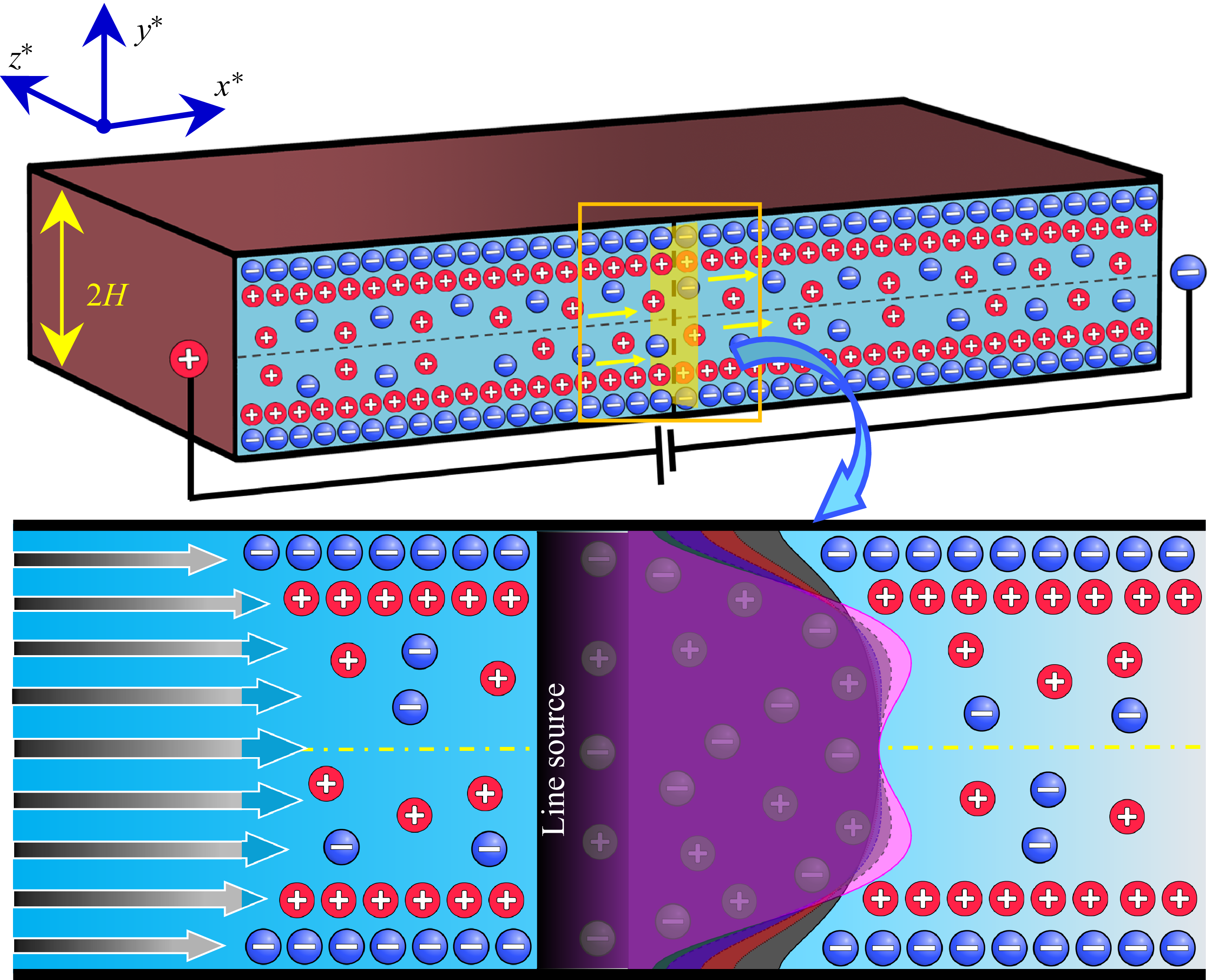
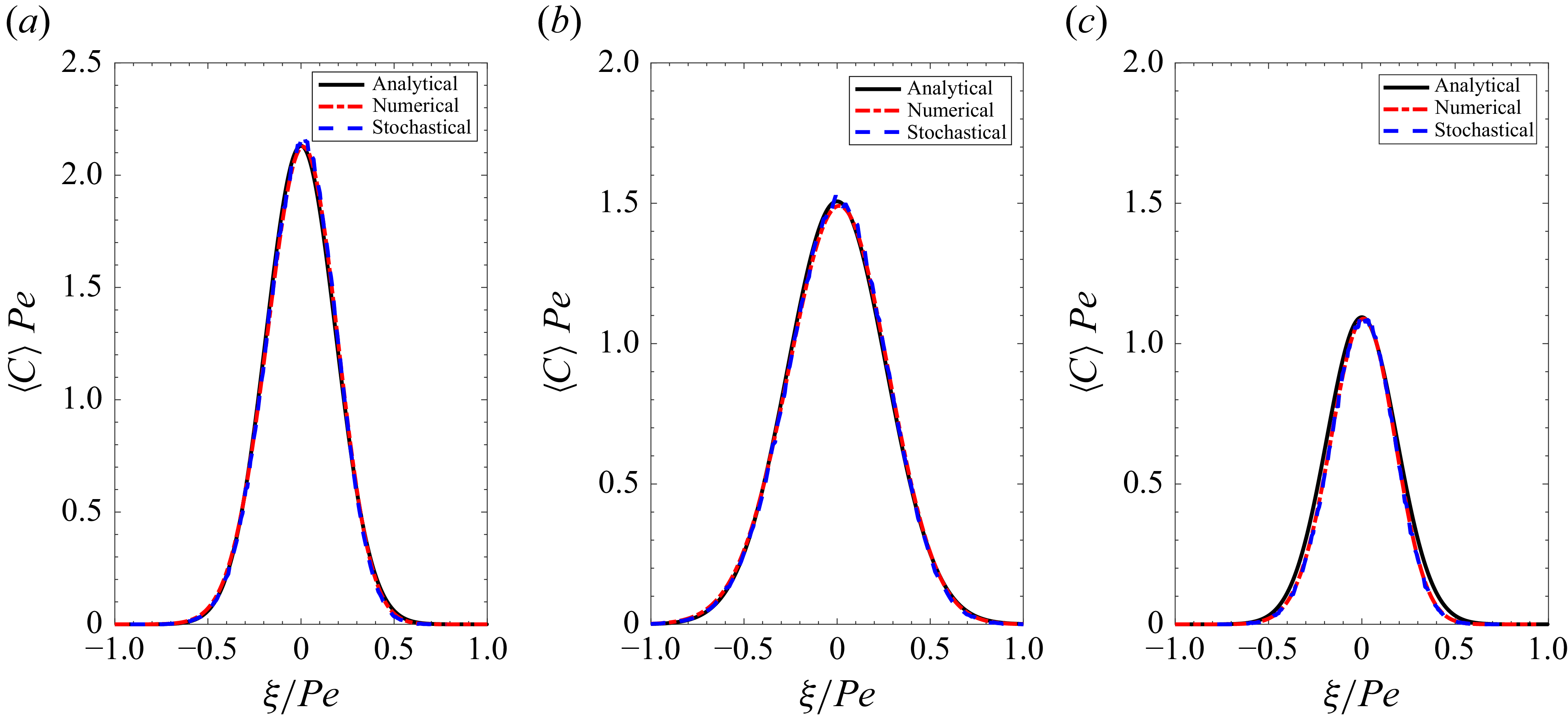


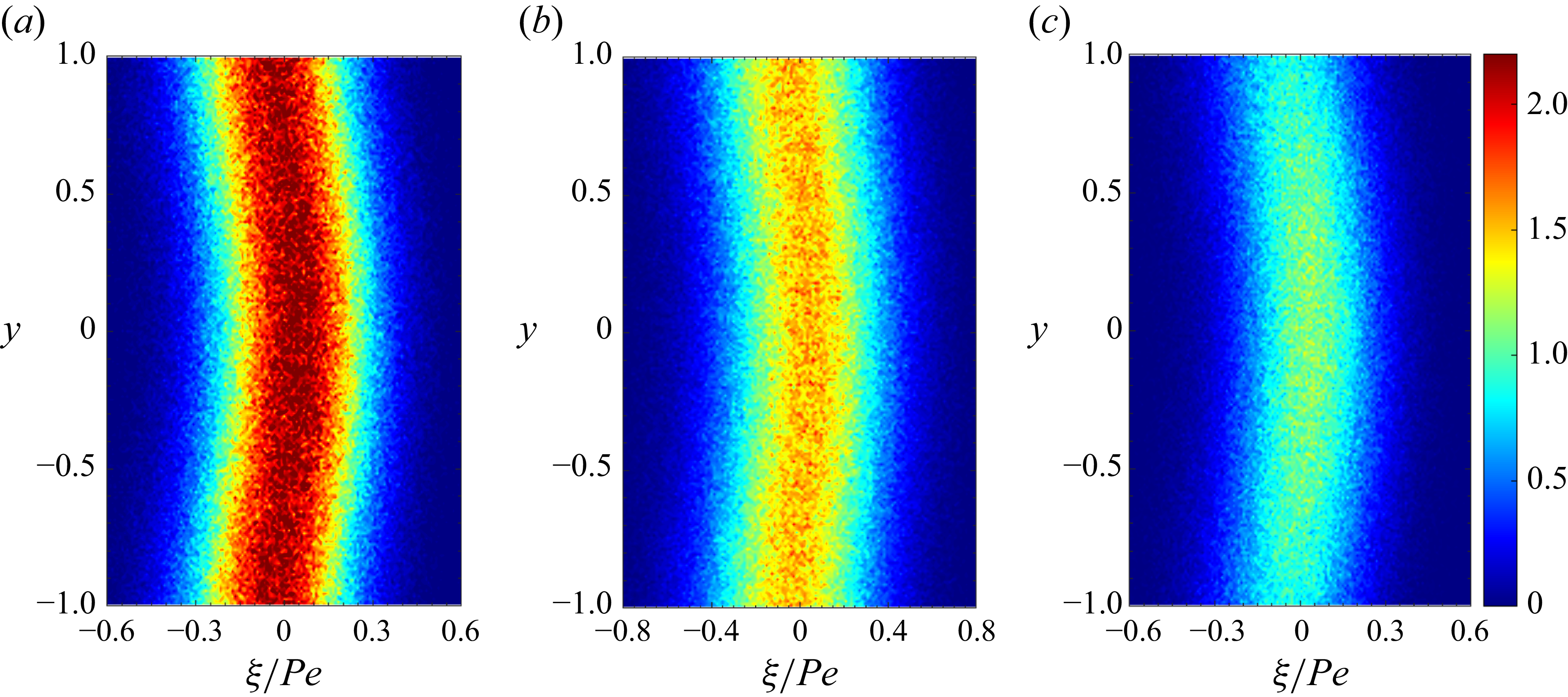


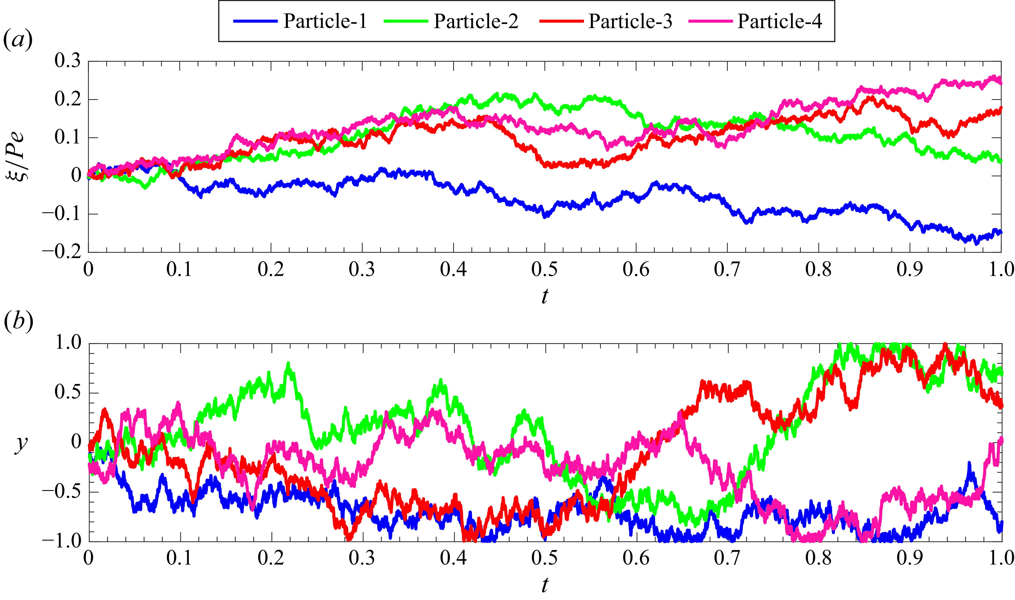


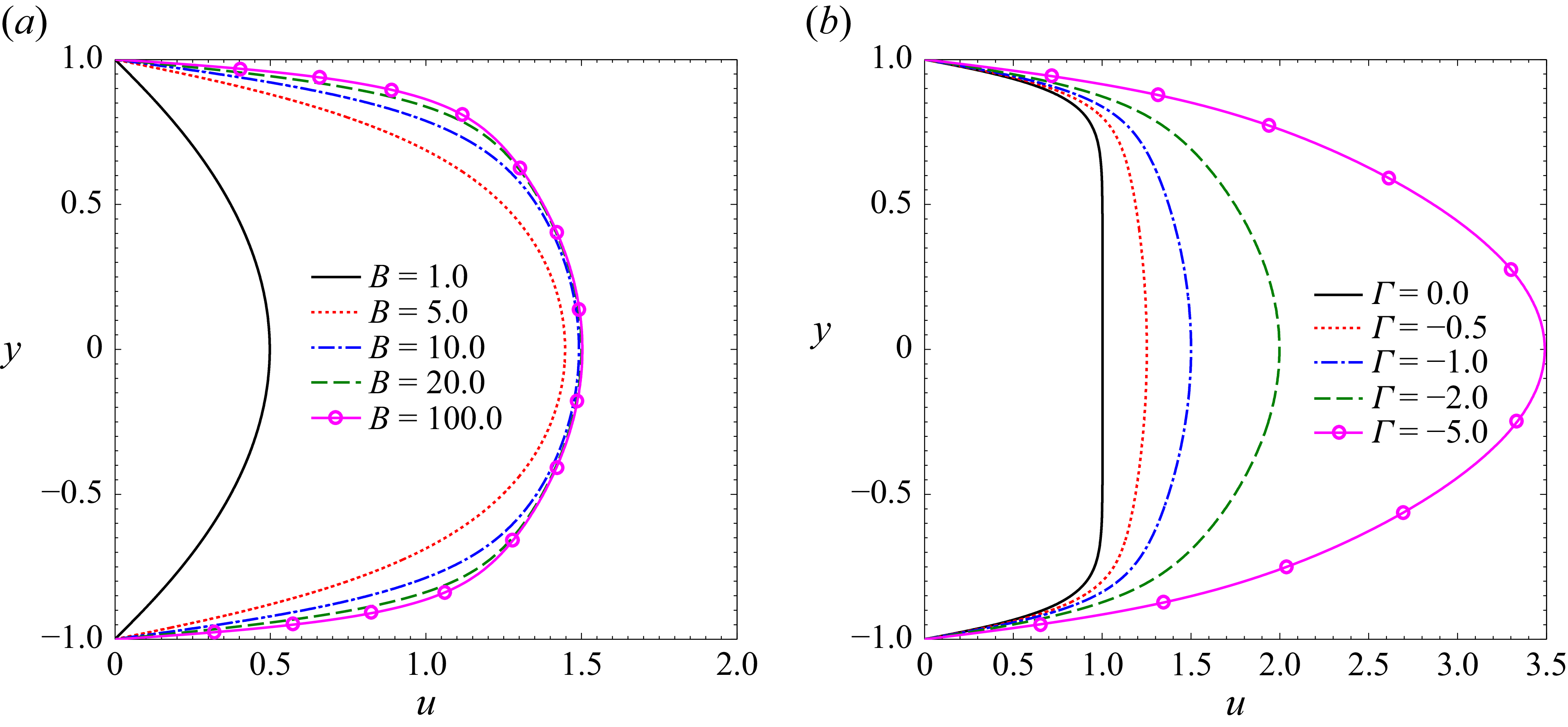


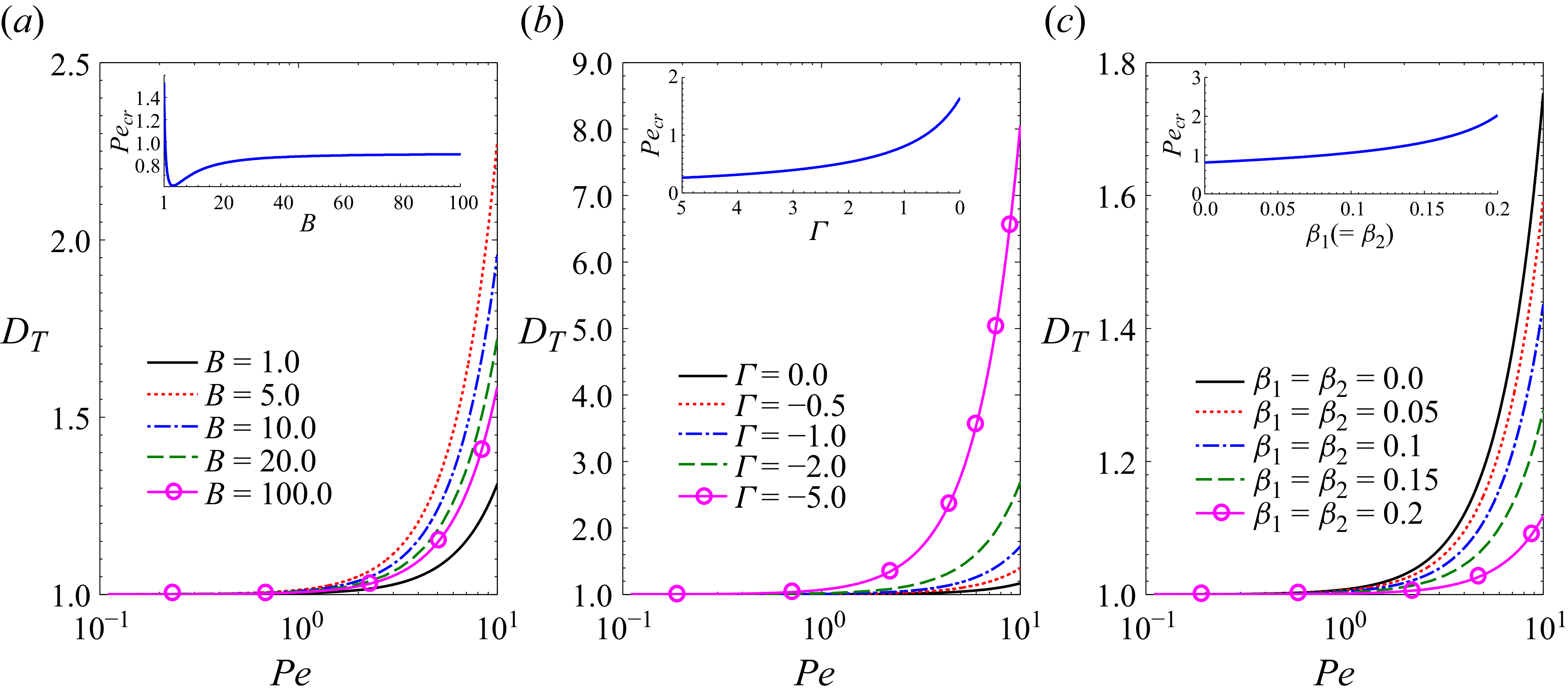


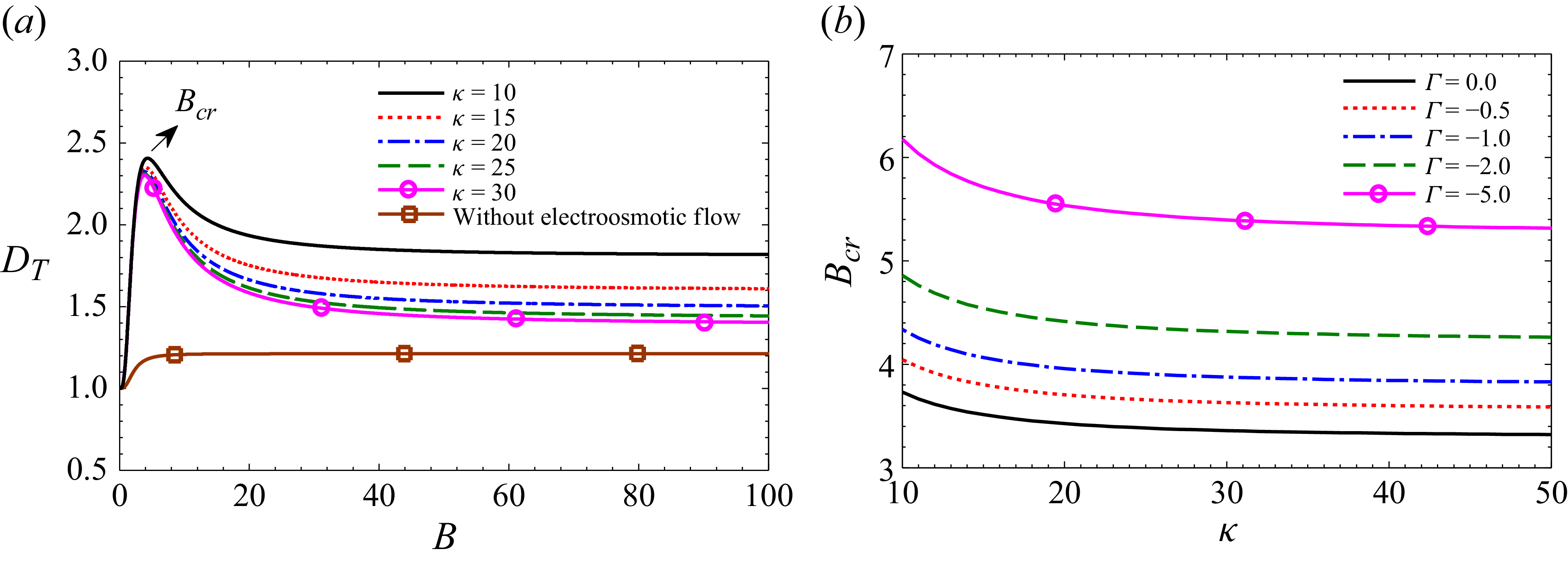


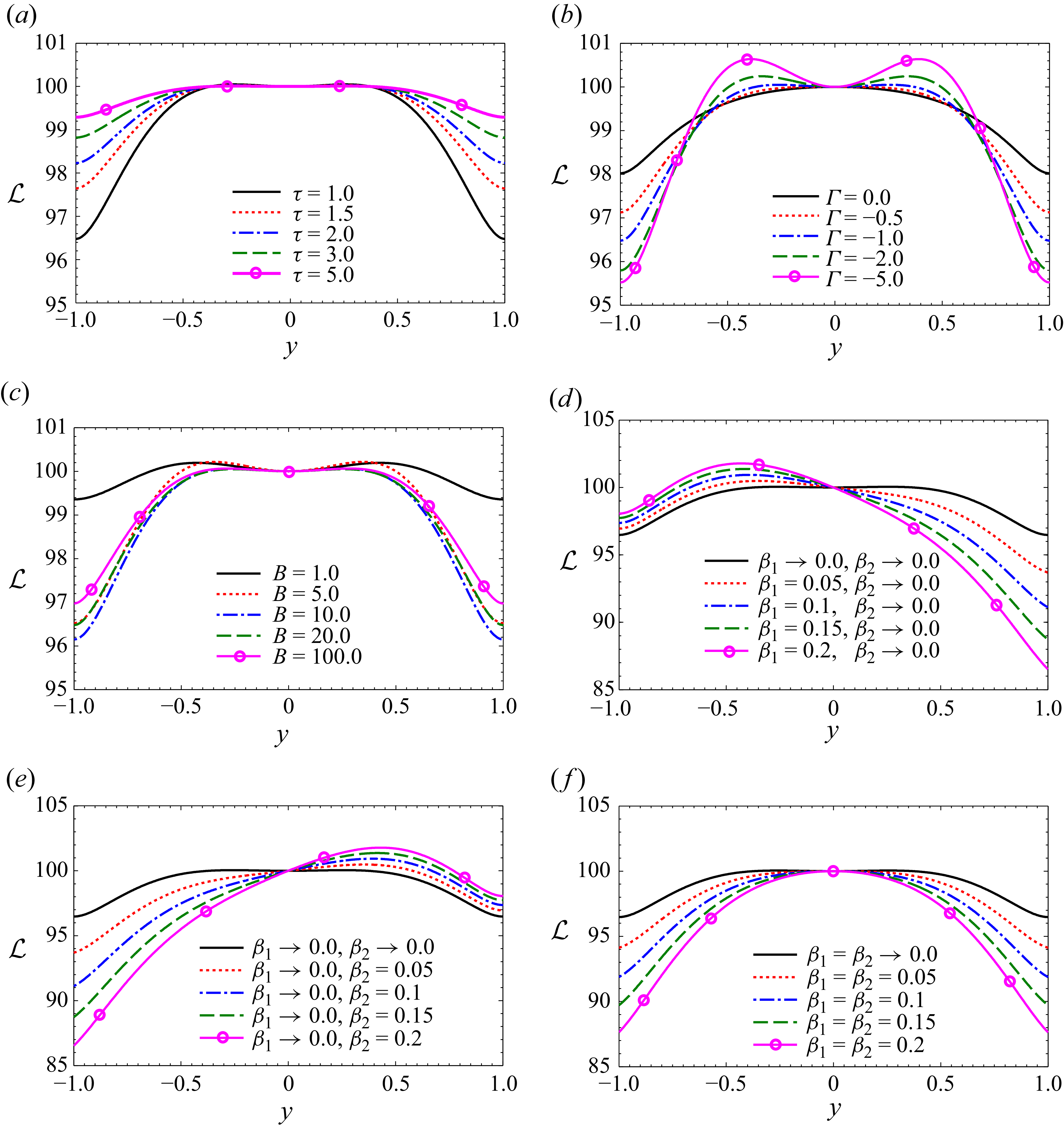


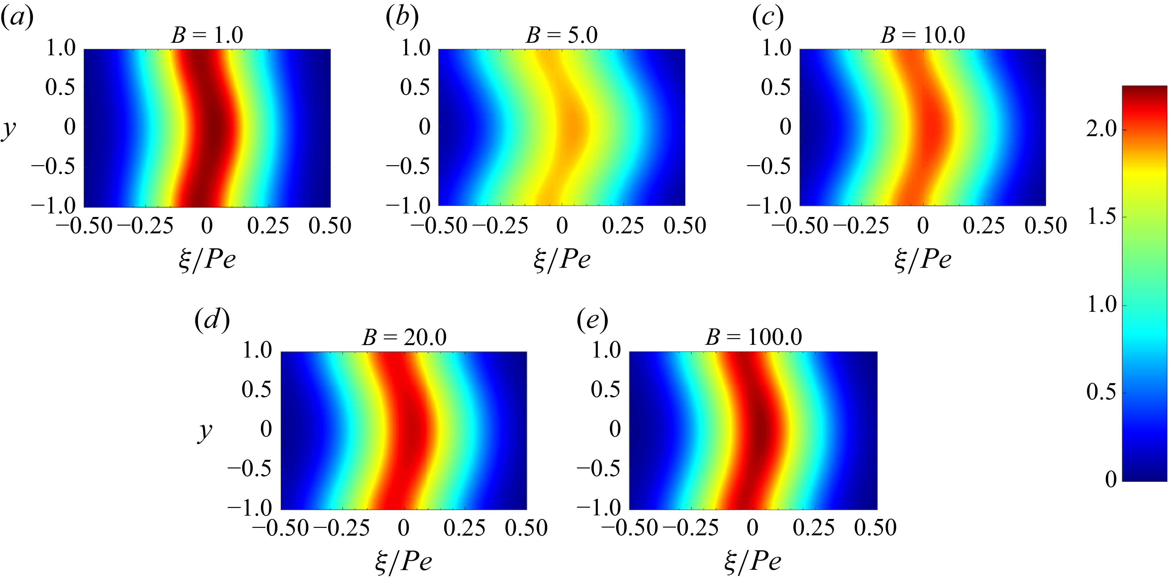


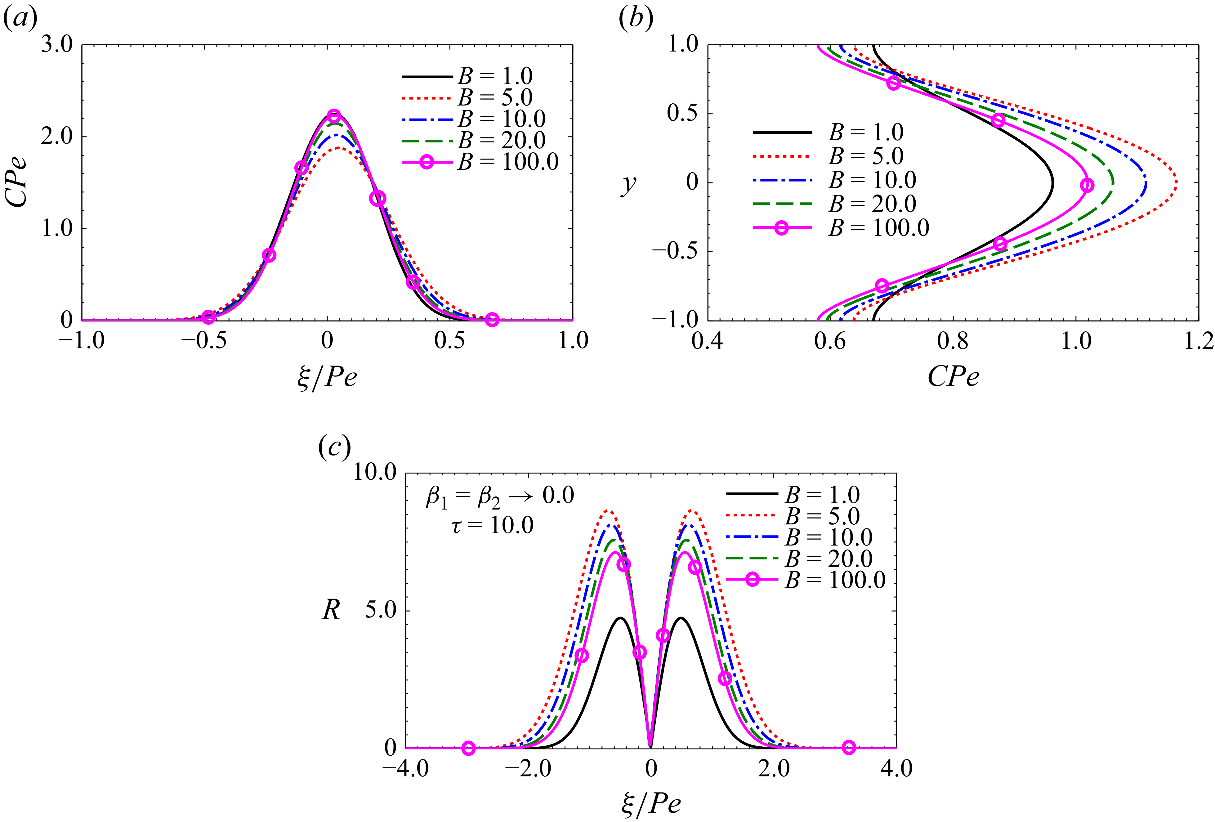


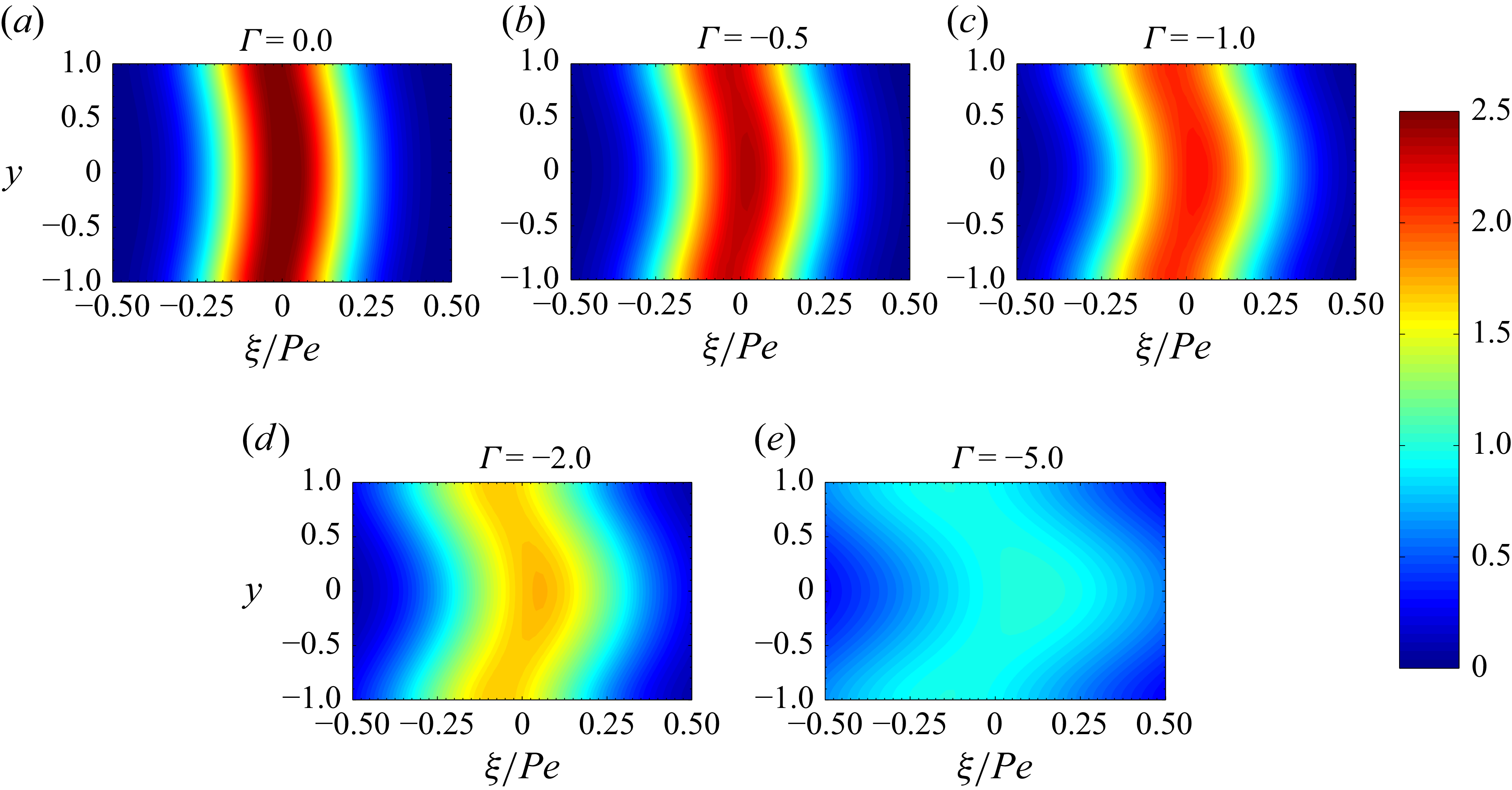


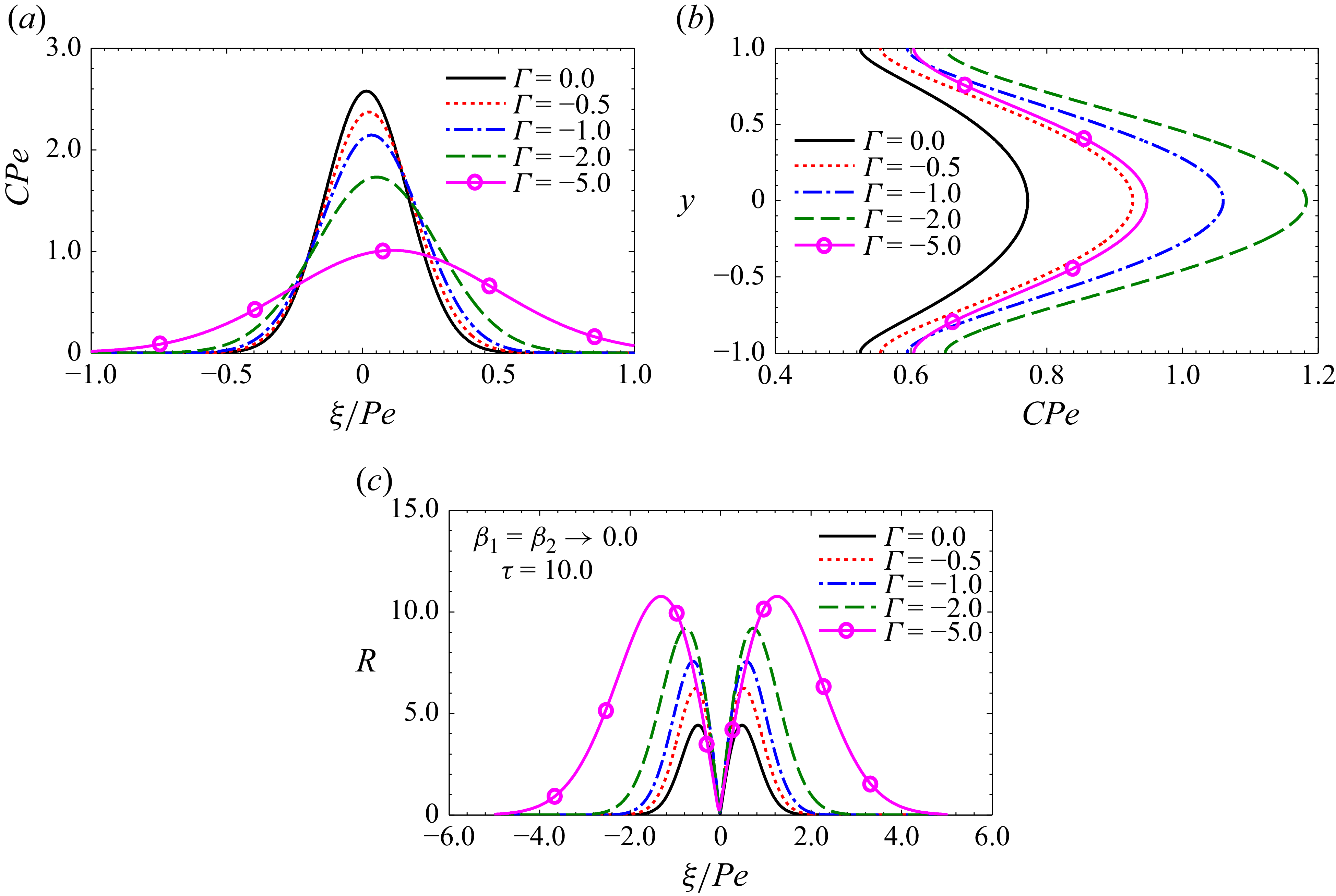


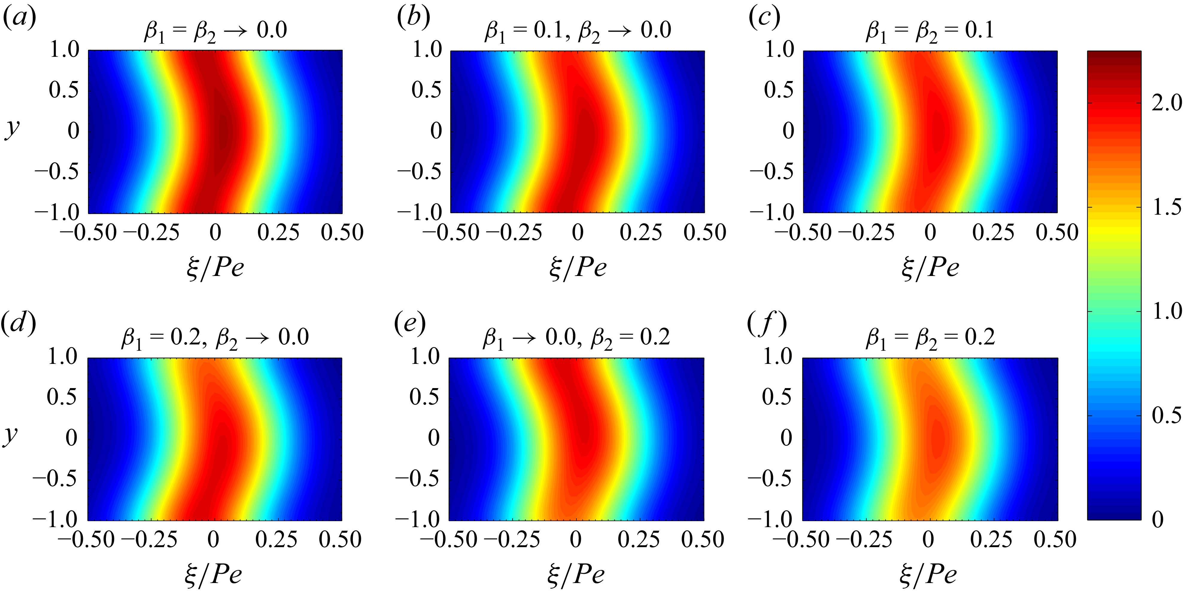


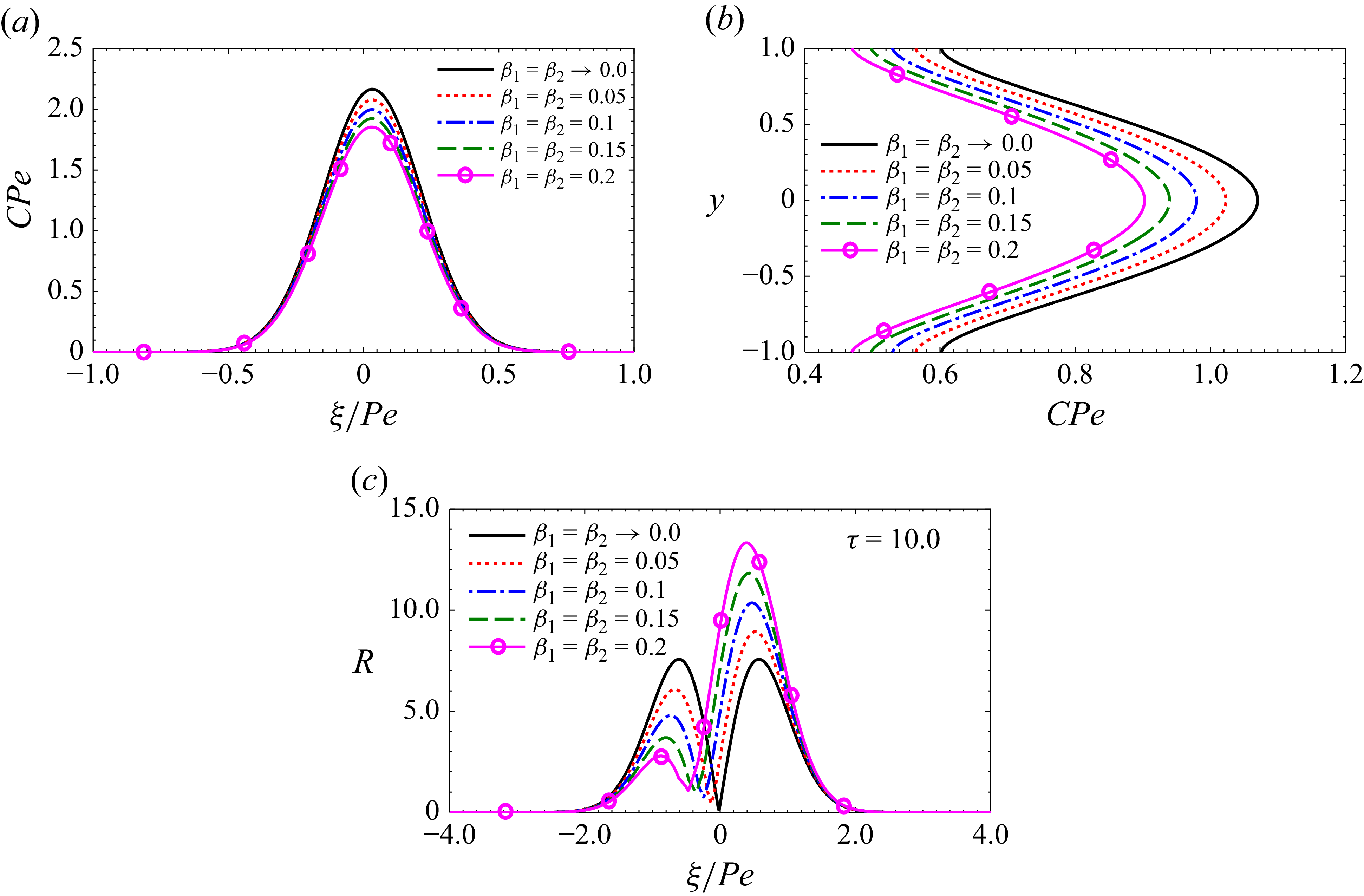


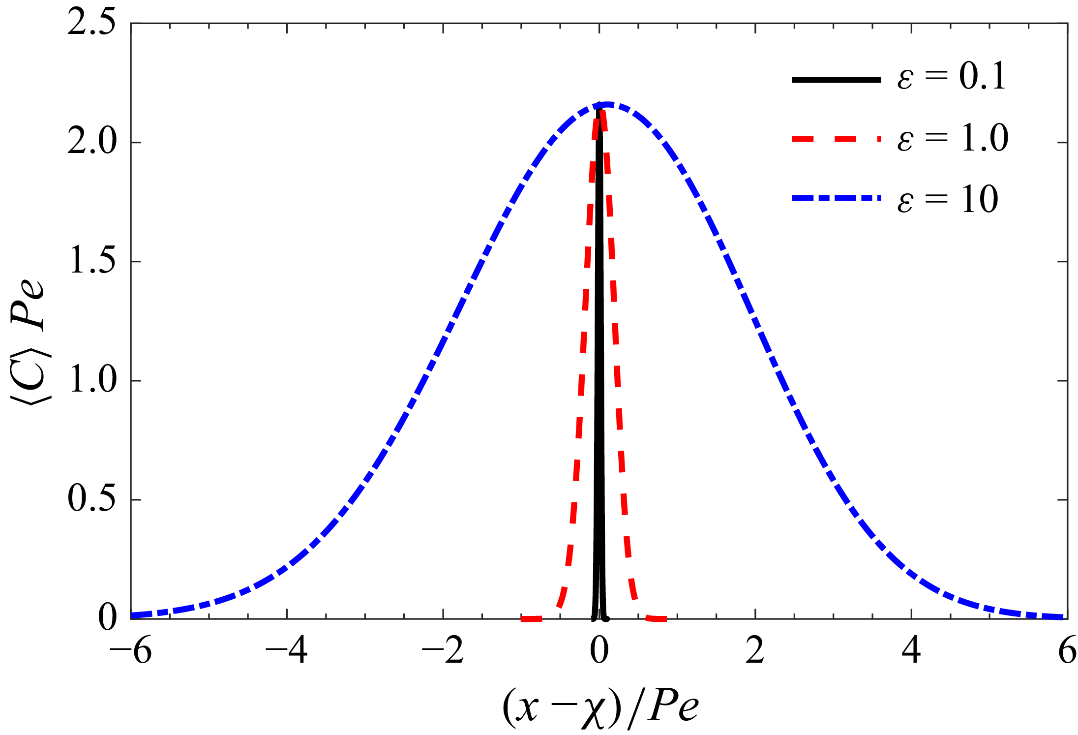


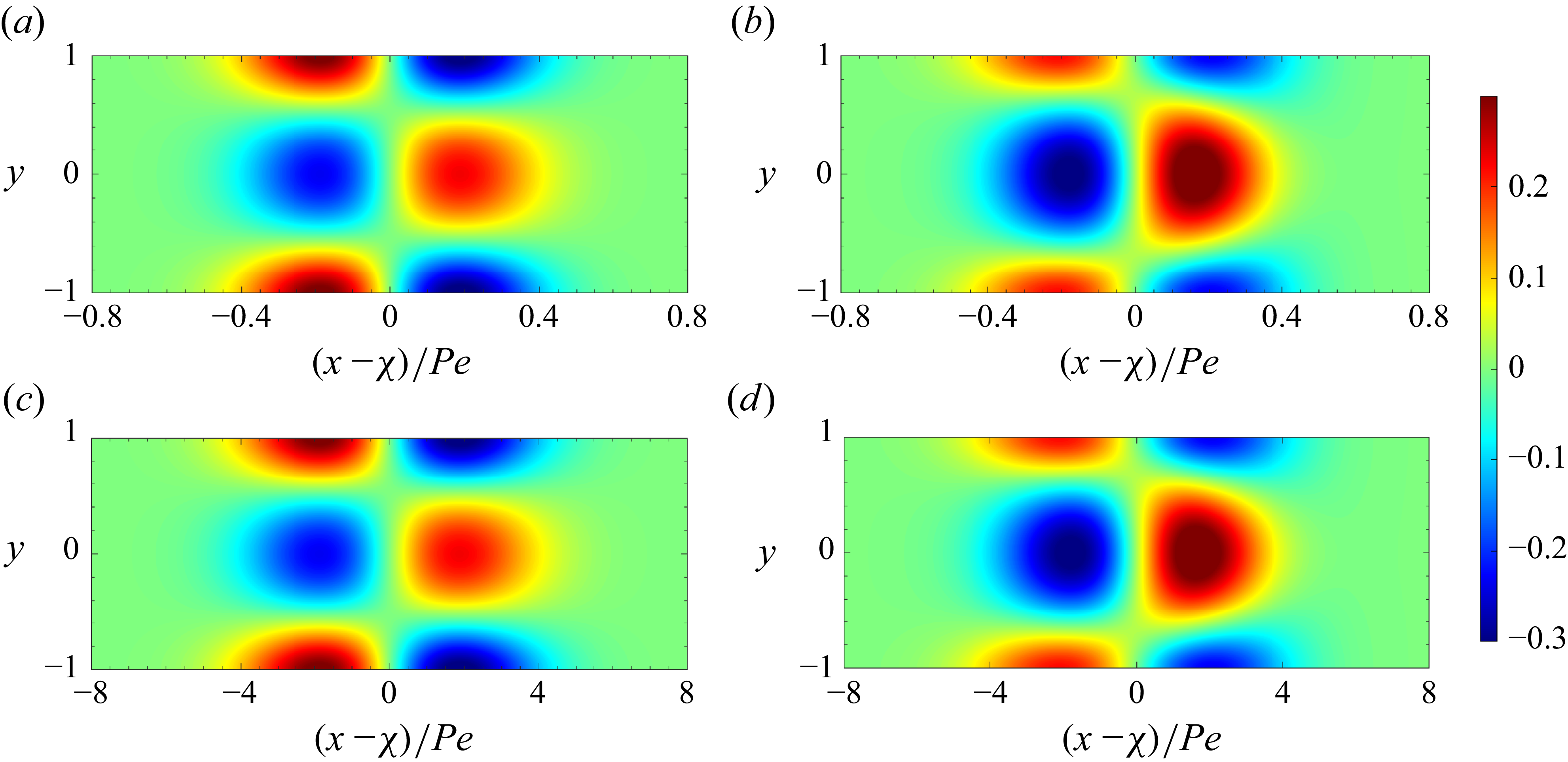


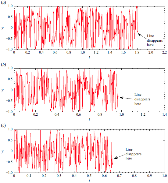


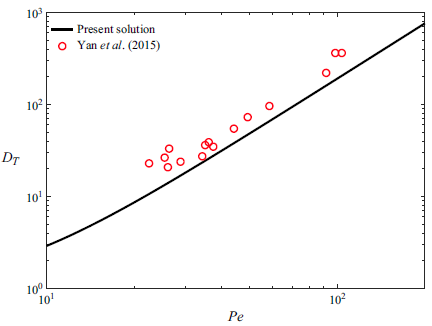


 Open access

