


1 Introduction
The tide in the ocean can readily be predicted, as it constitutes a direct response to the harmonic movement of the celestial bodies (Foreman Reference Foreman1996; Ray, Egbert & Erofeeva Reference Ray, Egbert and Erofeeva2011). Unlike ocean tides, tides in rivers are modulated by variable rainfall runoff (Hoitink & Jay Reference Hoitink and Jay2016). While the tide propagates up river, its amplitude and phase are modified by changes in the cross-section geometry (Green Reference Green1838) as well as by friction (Lorentz Reference Lorentz1926; Ippen Reference Ippen1966). A decrease in the cross-sectional area increases the amplitudes of surface elevation and velocity, while friction has the opposite effect (Jay Reference Jay1991; Savenije et al. Reference Savenije, Toffolon, Haas and Veling2008). Eventually, far upstream, friction prevails and the tidal wave diminishes. It decays the more rapidly, the stronger the river flow (LeBlond Reference LeBlond1978; Godin Reference Godin1985). The cross-section geometry is conventionally considered to be constant (Savenije et al. Reference Savenije, Toffolon, Haas and Veling2008), with the exception of tidal flats in some studies (e.g. Friedrichs & Madsen Reference Friedrichs and Madsen1992). While this assumption holds for strongly width-converging estuaries, it is inappropriate for long rivers with little variation of width. Here, the sloping river bed (Seminara, Pittaluga & Tambroni Reference Seminara, Pittaluga, Tambroni, Rodi and Uhlmann2012), as well as the seasonal variation of river discharge (Dai & Trenberth Reference Dai and Trenberth2002) lead to strongly different backwater profiles throughout the year. Based on a theoretical analysis, this contribution explains why backwater dynamics causes the tide to propagate very differently between periods of high and low river flow. During high flow, the tidal range decreases exponentially along the channel. During low flow, the convergence of the depth into the upstream direction causes the tidal range to decrease less rapidly along the downstream part of the tidal river, while the shallow depth causes the tidal range to decrease more rapidly along the upstream part of the tidal river.
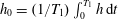
Idealized geometry of a tidal river: the width
 $w$
and bed slope
$w$
and bed slope
 $\unicode[STIX]{x2202}z_{b}/\unicode[STIX]{x2202}x$
remain constant along the river, except for the short funnel-shaped section that connects the river to the sea. The tidally averaged surface elevation
$\unicode[STIX]{x2202}z_{b}/\unicode[STIX]{x2202}x$
remain constant along the river, except for the short funnel-shaped section that connects the river to the sea. The tidally averaged surface elevation
 $z_{0}$
(dashed) depends on the river discharge
$z_{0}$
(dashed) depends on the river discharge
 $Q_{0}$
. It forms a backwater profile (black) when the river discharge is low and a drawdown curve when the river discharge is high (blue). Both the tidally averaged depth
$Q_{0}$
. It forms a backwater profile (black) when the river discharge is low and a drawdown curve when the river discharge is high (blue). Both the tidally averaged depth
 $h_{0}$
and tidal amplitude
$h_{0}$
and tidal amplitude
 $|z_{1}|$
gradually vary along the channel depending on the river discharge. For normal flow (
$|z_{1}|$
gradually vary along the channel depending on the river discharge. For normal flow (
 $Q_{0}=Q_{n}$
) (green), the tidally averaged depth remains constant along the river
$Q_{0}=Q_{n}$
) (green), the tidally averaged depth remains constant along the river
 $(\unicode[STIX]{x2202}h/\unicode[STIX]{x2202}x=\unicode[STIX]{x2202}z_{s}/\unicode[STIX]{x2202}x-\unicode[STIX]{x2202}z_{b}/\unicode[STIX]{x2202}x=0)$
.
$(\unicode[STIX]{x2202}h/\unicode[STIX]{x2202}x=\unicode[STIX]{x2202}z_{s}/\unicode[STIX]{x2202}x-\unicode[STIX]{x2202}z_{b}/\unicode[STIX]{x2202}x=0)$
.

River tides are described by the nonlinear shallow-water equations, which, in general, do not admit a closed-form solution. Theoretical insight into river tides, therefore, builds on simplifications of the underlying equations, as well as a reduced complexity of the river geometry. We focus here on tidal rivers that form long channels of nearly constant width. Seasonally averaged, the net discharge of a tidal river is stronger than that of the tide, so that the flow does not reverse, and where the water remains fresh (Godin Reference Godin1985). Tidal rivers are connected to the sea by a short, width-converging reach, the tidal funnel (figure 1), where the tidal influence is considerable even during periods of strong river flow. The tide travels up the river at a length that exceeds many times the length of the funnel. This geometry sets tidal rivers apart from tidally dominated estuaries that strongly converge in width along their entire length and have brackish water (Pritchard Reference Pritchard and Lauff1967). The bed of long non-converging estuaries is typically horizontal (Savenije Reference Savenije2015) except at the mouth, where there are shallow sandbars. Idealized models thus represent tidal rivers as non-converging channels with a horizontal bed, along which width and depth remain constant (Godin Reference Godin1985, Reference Godin1991a ).
The dependence of the water depth on the river discharge is commonly ignored in models of tidal propagation (Godin Reference Godin1984; Horrevoets et al. Reference Horrevoets, Savenije, Schuurman and Graas2004; Savenije et al. Reference Savenije, Toffolon, Haas and Veling2008). This allows for an analytic solution of the propagation of tidal waves up river, with an amplitude that is much smaller than the water depth (Godin Reference Godin1991a ). If there is no river flow, then the tide is gradually damped and delayed proportionally to the tidal amplitude and the amplitude decreases exponentially along the channel (Ippen Reference Ippen1966; Friedrichs Reference Friedrichs and Valle-Levinson2010). River discharge superimposes a mean flow velocity so that friction increases. The tidal amplitude still decreases exponentially when the river flow is strong, but at a higher rate that is proportional to the square root of the mean flow velocity (LeBlond Reference LeBlond1978; Godin Reference Godin1985, Reference Godin1991a ; Jay Reference Jay1991; Jay & Flinchem Reference Jay and Flinchem1997; Godin Reference Godin1999; Alebregtse & de Swart Reference Alebregtse and de Swart2016). Even the few models that do consider the water level set-up neglect the slope of the bed (Cai, Savenije & Toffolon Reference Cai, Savenije and Toffolon2014). However, the bed of tidal rivers typically slopes up beyond the upstream end of tidal funnels (Seminara et al. Reference Seminara, Pittaluga, Tambroni, Rodi and Uhlmann2012; Kästner et al. Reference Kästner, Hoitink, Vermeulen, Geertsema and Ningsih2017). It is well known that the rising river bed limits the tidal intrusion approximately to the point where the bed reaches sea level (Dalrymple et al. Reference Dalrymple, Kurcinka, Jablonski, Ichaso and Mackay2015; Nienhuis, Hoitink & Törnqvist Reference Nienhuis, Hoitink and Törnqvist2018). Here, we demonstrate that this limit is not because the waves cannot run up the slope, but rather because friction is always strong in the upstream part of the tidal river. The sloping bed causes the tidally averaged water depth to gradually vary along the river except for periods where the river is at normal flow, when the water surface slope is identical to the bed slope (figure 1). The depth can thus converge over a long distance, even though the width may only converge along the short tidal funnel. This contribution explores the implications of systematic depth variations.
Our study is motivated by observations in the Kapuas River, Indonesia, which features a seasonal backwater variation that strongly influences tidal propagation. These observations are not well predicted by conventional models that do not take the backwater effect into account. This paper extends the conceptual understanding of river tides by providing a theoretical model that explains how the tide propagates along a backwater affected river, such as the Kapuas. Section 2 presents observations of the tide and backwater variation in the Kapuas River. Section 3 develops a general theory of river tides, following the classical approach by transforming the shallow-water equations into the wave equation (Lamb Reference Lamb1932; Dronkers Reference Dronkers1964; Ippen Reference Ippen1966; Parker Reference Parker1984). We show that the propagation of the tide along a channel with varying geometry can be interpreted as the transmission and reflection at a sequence of infinitesimal steps. This analogy is used to determine the damping and celerity of the tidal wave along a channel with a gradually varying cross-section geometry. Based on the theory developed in § 3, § 4 shows how the tide propagates along a river with a sloping bed. Section 5 discusses the main results, and in § 6, conclusions are drawn.
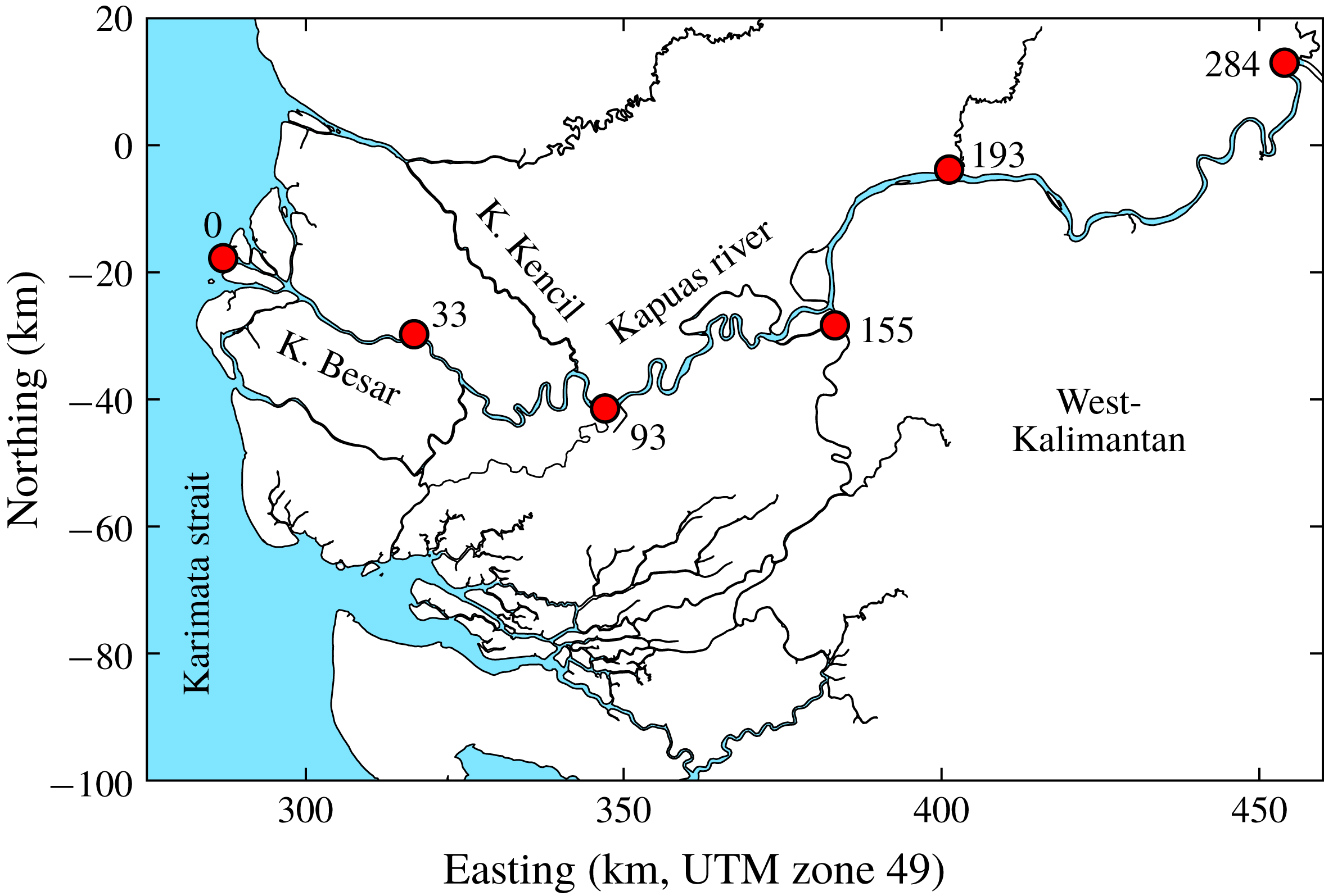
Coastal zone of the Kapuas River: selected gauging stations are labelled with their respective distance to the river mouth.
2 Tidal propagation along the Kapuas River
The Kapuas River is located in West Kalimantan, Indonesia (figure 2). The catchment is situated in the humid tropics so that the river discharge varies strongly with the monsoon (Kästner et al. Reference Kästner, Hoitink, Torfs, Vermeulen, Ningsih and Pramulya2018). The bed of the Kapuas is moderately sloping (Kästner et al. Reference Kästner, Hoitink, Vermeulen, Geertsema and Ningsih2017). These conditions result in different backwater profiles between the wet and the dry season, which in turn strongly affect the propagation of the tide. The Kapuas River has one large distributary, from which three smaller distributaries branch off. The smaller distributaries only slightly affect the tide in the main stem of the river. Due to the microtidal regime, the distributaries only funnel along a short reach close to the sea. This renders the Kapuas an ideal case to study the propagation of tides along a backwater affected tidal river.
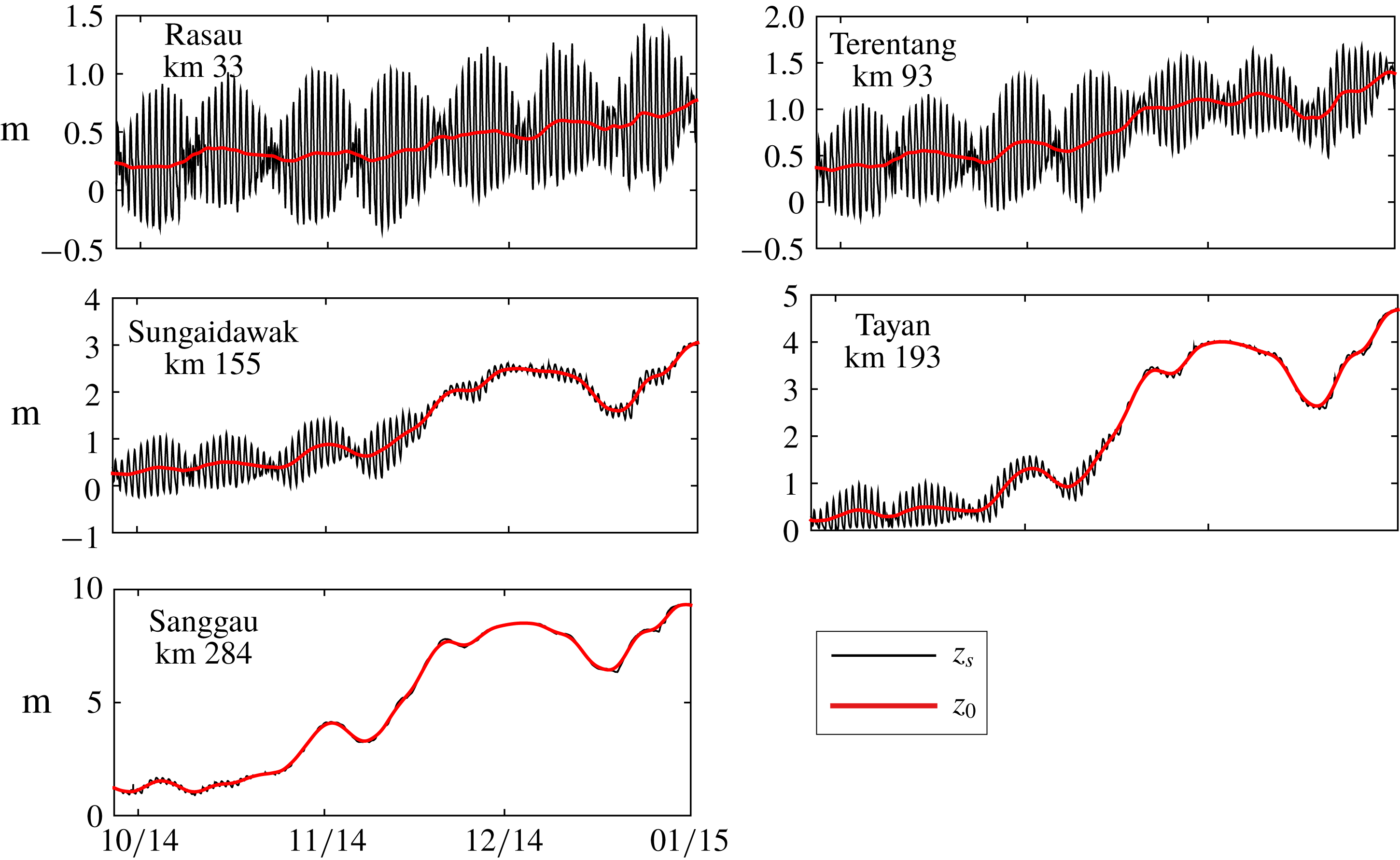
The tidally averaged water surface forms a pronounced backwater profile during low flow but remains nearly parallel to the river bed during high flow (figure 4
a). The tidally averaged water level increases with the river discharge the further that a station is located from the sea. The tidally averaged water level ranges over 10 m at Sanggau, 285 km from the sea, but only by 2 m at Mendawat, 130 km from the sea. The tidal range decreases with the distance from the coast and with the river discharge (figures 3 and 4
b). At high flow, the damping is nearly exponential, and the tidal range drops to half the initial value at 50 km. For lower discharges, the admittance, i.e. the ratio of the tidal surface elevation amplitude along the river and the amplitude at the river mouth, is higher. During low flow, the shape of the admittance along the river is very different from that of a decaying exponential. Close to 150 km, the admittance has a knickpoint, where the damping strongly increases. Up to this point, the tidal amplitude is isosynchronous, i.e. remains constant during low flow. Below a river discharge of
 $5000~\text{m}^{3}~\text{s}^{-1}$
, the tide becomes noticeable at Sanggau. At extremely low flow, the tidal range at Sanggau is still half as large as the range at sea. Conventional tidal models that do not include the backwater effect predict that the tidal admittance decreases exponentially with increasing distance from the sea and thus fail to explain the observed isosynchronous admittance during low flow. The following section extends the theory of river tides by variable backwater effects, which predicts the tide in agreement with the observation.
$5000~\text{m}^{3}~\text{s}^{-1}$
, the tide becomes noticeable at Sanggau. At extremely low flow, the tidal range at Sanggau is still half as large as the range at sea. Conventional tidal models that do not include the backwater effect predict that the tidal admittance decreases exponentially with increasing distance from the sea and thus fail to explain the observed isosynchronous admittance during low flow. The following section extends the theory of river tides by variable backwater effects, which predicts the tide in agreement with the observation.
Time series of the surface elevation
 $z_{s}$
(black) and its tidal average
$z_{s}$
(black) and its tidal average
 $z_{0}$
(red) at five gauging stations along the Kapuas River;
$z_{0}$
(red) at five gauging stations along the Kapuas River;
 $z_{0}$
is determined by low pass filtering with a cutoff period of one tidal cycle so that the subtidal variation over the spring-neap cycle remains.
$z_{0}$
is determined by low pass filtering with a cutoff period of one tidal cycle so that the subtidal variation over the spring-neap cycle remains.
(a) Observed tidally averaged water level and (b) admittance of tidal range along the Kapuas River at different river discharges.

3 Generic model of river tides
3.1 Tidal waves
The tide causes the water surface elevation
 $z_{s}$
and discharge
$z_{s}$
and discharge
 $Q$
to periodically oscillate over time
$Q$
to periodically oscillate over time
 $t$
, which suggests separating them into the components
$t$
, which suggests separating them into the components
 $z_{j}=\text{Re}\{z_{j}\}$
and
$z_{j}=\text{Re}\{z_{j}\}$
and
 $Q_{j}=\text{Re}\{Q_{j}\}$
with frequencies
$Q_{j}=\text{Re}\{Q_{j}\}$
with frequencies
 $\unicode[STIX]{x1D714}_{j}$
(Godin Reference Godin1991b
),
$\unicode[STIX]{x1D714}_{j}$
(Godin Reference Godin1991b
),
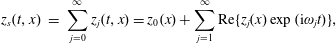 $$\begin{eqnarray}\displaystyle z_{s}(t,x) & = & \displaystyle \mathop{\sum }_{j=0}^{\infty }z_{j}(t,x)=z_{0}(x)+\mathop{\sum }_{j=1}^{\infty }\text{Re}\{z_{j}(x)\exp (\text{i}\unicode[STIX]{x1D714}_{j}t)\},\end{eqnarray}$$
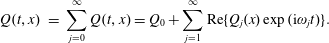 $$\begin{eqnarray}\displaystyle Q(t,x) & = & \displaystyle \mathop{\sum }_{j=0}^{\infty }Q(t,x)=Q_{0}+\mathop{\sum }_{j=1}^{\infty }\text{Re}\{Q_{j}(x)\exp (\text{i}\unicode[STIX]{x1D714}_{j}t)\}.\end{eqnarray}$$
 $x$
is omitted from the notation further on. The subscript
$x$
is omitted from the notation further on. The subscript
 $j$
denotes the frequency. The frequency components are determined by the inner product
$j$
denotes the frequency. The frequency components are determined by the inner product
 $(y)_{j}=(1/T)\int _{T}y(\cos \unicode[STIX]{x1D714}_{j}t+\text{i}\sin \unicode[STIX]{x1D714}_{j}t)\,\text{d}t$
, where the time
$(y)_{j}=(1/T)\int _{T}y(\cos \unicode[STIX]{x1D714}_{j}t+\text{i}\sin \unicode[STIX]{x1D714}_{j}t)\,\text{d}t$
, where the time
 $T$
is the least common multiple of all periods.
$T$
is the least common multiple of all periods. The surface elevation of each frequency component has a distinct amplitude
 $|z_{j}|$
and phase
$|z_{j}|$
and phase
 $\unicode[STIX]{x1D711}_{jz}=\arctan (\text{Im}(z_{j})/\text{Re}\{z_{j}\})$
. The astronomical tide consists of an infinite number of constituents (Pugh Reference Pugh1987). Their frequencies are integer combinations of basic frequencies derived from the orbits of the celestial bodies (Doodson Reference Doodson1921; Cartwright & Tayler Reference Cartwright and Tayler1971; Souchay, Mathis & Tokieda Reference Souchay, Mathis and Tokieda2012). Several dozen constituents are required to accurately predict ocean tides, of which many constituents are of similar frequency and magnitude. Long time series are required to separate these constituents from each other.
$\unicode[STIX]{x1D711}_{jz}=\arctan (\text{Im}(z_{j})/\text{Re}\{z_{j}\})$
. The astronomical tide consists of an infinite number of constituents (Pugh Reference Pugh1987). Their frequencies are integer combinations of basic frequencies derived from the orbits of the celestial bodies (Doodson Reference Doodson1921; Cartwright & Tayler Reference Cartwright and Tayler1971; Souchay, Mathis & Tokieda Reference Souchay, Mathis and Tokieda2012). Several dozen constituents are required to accurately predict ocean tides, of which many constituents are of similar frequency and magnitude. Long time series are required to separate these constituents from each other.
River discharge not only determines the means
 $z_{0}$
and
$z_{0}$
and
 $Q_{0}$
(
$Q_{0}$
(
 $\unicode[STIX]{x1D714}_{0}=0$
) but also modulates the tide. River discharge varies in an irregular manner over much shorter periods than necessary for a meaningful harmonic analysis. Therefore, we consider the tide for successive periods of just one tidal cycle and decompose it into a Fourier series, where the frequencies of the components are integer multiples of a single fundamental frequency,
$\unicode[STIX]{x1D714}_{0}=0$
) but also modulates the tide. River discharge varies in an irregular manner over much shorter periods than necessary for a meaningful harmonic analysis. Therefore, we consider the tide for successive periods of just one tidal cycle and decompose it into a Fourier series, where the frequencies of the components are integer multiples of a single fundamental frequency,
 $\unicode[STIX]{x1D714}_{j}=j\unicode[STIX]{x1D714}_{1}$
. The Fourier components decay rapidly in amplitude, which allows a meaningful truncation of the series to just a few components. These components are referred to as tidal species and effectively lump tidal constituents of similar frequencies together (Kukulka & Jay Reference Kukulka and Jay2003b
; Guo et al.
Reference Guo, van der Wegen, Jay, Matte, Wang, Roelvink and He2015). Alternatively to species, the tidal wave can be interpreted as a periodic function of arbitrary shape that is described by low water and high water (Savenije Reference Savenije2001; Savenije et al.
Reference Savenije, Toffolon, Haas and Veling2008). This approach is supported by the observation that tidal waves travel upstream individually after each other and that the discharge of large rivers changes little over the time it takes a single wave to travel upstream. The incoming tide is thus roughly represented by a single frequency component that has an amplitude equal to half the tidal range. The range of the incoming tide changes from one tidal cycle to the next, most notably over to the spring-neap cycle. The river tide has therefore be predicted for each cycle individually, depending on the incoming tide and the river flow. The amplitude and phase of a wave change as a wave propagates up river, depending on the cross-section geometry and river discharge. For convenience, this is expressed in the form of the admittance
$\unicode[STIX]{x1D714}_{j}=j\unicode[STIX]{x1D714}_{1}$
. The Fourier components decay rapidly in amplitude, which allows a meaningful truncation of the series to just a few components. These components are referred to as tidal species and effectively lump tidal constituents of similar frequencies together (Kukulka & Jay Reference Kukulka and Jay2003b
; Guo et al.
Reference Guo, van der Wegen, Jay, Matte, Wang, Roelvink and He2015). Alternatively to species, the tidal wave can be interpreted as a periodic function of arbitrary shape that is described by low water and high water (Savenije Reference Savenije2001; Savenije et al.
Reference Savenije, Toffolon, Haas and Veling2008). This approach is supported by the observation that tidal waves travel upstream individually after each other and that the discharge of large rivers changes little over the time it takes a single wave to travel upstream. The incoming tide is thus roughly represented by a single frequency component that has an amplitude equal to half the tidal range. The range of the incoming tide changes from one tidal cycle to the next, most notably over to the spring-neap cycle. The river tide has therefore be predicted for each cycle individually, depending on the incoming tide and the river flow. The amplitude and phase of a wave change as a wave propagates up river, depending on the cross-section geometry and river discharge. For convenience, this is expressed in the form of the admittance
 $|z_{j}(x)|/|z_{j}(0)|$
and phase difference
$|z_{j}(x)|/|z_{j}(0)|$
and phase difference
 $\unicode[STIX]{x1D711}_{jz}(x)-\unicode[STIX]{x1D711}_{jz}(0)$
, where
$\unicode[STIX]{x1D711}_{jz}(x)-\unicode[STIX]{x1D711}_{jz}(0)$
, where
 $x$
is the distance from the river mouth. The remainder of this section develops the theory of tidal wave propagation. It builds on previous works by Godin (Reference Godin1985) and Jay (Reference Jay1991). This section advances the theory on how tides propagate along rivers with varying cross-section geometry. The theory is held general and covers both mild depth and width convergence. Section 4 then analyses the backwater effect caused by a varying river discharge and a sloping bed.
$x$
is the distance from the river mouth. The remainder of this section develops the theory of tidal wave propagation. It builds on previous works by Godin (Reference Godin1985) and Jay (Reference Jay1991). This section advances the theory on how tides propagate along rivers with varying cross-section geometry. The theory is held general and covers both mild depth and width convergence. Section 4 then analyses the backwater effect caused by a varying river discharge and a sloping bed.
3.2 Shallow-water equations
The flow in open channels is described by the one-dimensional shallow-water equations (Cunge, Holly & Verwey Reference Cunge, Holly and Verwey1980; Savenije Reference Savenije2012). These are the equation of continuity,
 $$\begin{eqnarray}\frac{\unicode[STIX]{x2202}A}{\unicode[STIX]{x2202}t}+\frac{\unicode[STIX]{x2202}Q}{\unicode[STIX]{x2202}x}=0,\end{eqnarray}$$
as well as the equation of motion,
 $$\begin{eqnarray}\frac{\unicode[STIX]{x2202}Q}{\unicode[STIX]{x2202}t}+\frac{\unicode[STIX]{x2202}}{\unicode[STIX]{x2202}x}\left(\frac{Q^{2}}{A}\right)+\frac{1}{2}\frac{g}{w}\frac{\unicode[STIX]{x2202}A^{2}}{\unicode[STIX]{x2202}x}=-gA\frac{\unicode[STIX]{x2202}z_{b}}{\unicode[STIX]{x2202}x}+g\frac{A^{2}}{w^{2}}\frac{\unicode[STIX]{x2202}w}{\unicode[STIX]{x2202}x}-c_{d}w\frac{Q|Q|}{A^{2}},\end{eqnarray}$$
where
 $A$
is the cross-sectional area,
$A$
is the cross-sectional area,
 $Q$
the discharge,
$Q$
the discharge,
 $w$
the channel width,
$w$
the channel width,
 $z_{b}$
the bed level,
$z_{b}$
the bed level,
 $g$
the gravitational acceleration and
$g$
the gravitational acceleration and
 $c_{d}$
the drag coefficient. We analyse here only the case of a straight non-meandering channel that has a rectangular cross-section, i.e. no intertidal areas (figure 1), so that the depth
$c_{d}$
the drag coefficient. We analyse here only the case of a straight non-meandering channel that has a rectangular cross-section, i.e. no intertidal areas (figure 1), so that the depth
 $h=A/w$
and the surface elevation
$h=A/w$
and the surface elevation
 $z_{s}=z_{b}+h$
. The terms on the right-hand side in (3.2b
) represent the forces acting on the flow per unit distance along the channel. The forces determine how the tidal wave changes while propagating up river. Tidal flats are not taken into account, as intertidal areas are small in rivers. The reader is referred to Speer & Aubrey (Reference Speer and Aubrey1985), Jay (Reference Jay1991), Friedrichs & Madsen (Reference Friedrichs and Madsen1992), Savenije et al. (Reference Savenije, Toffolon, Haas and Veling2008) for the treatment of intertidal storage, and for tidal propagation along channels of arbitrary cross-sections, to Li & Valle-Levinson (Reference Li and Valle-Levinson1999). We assume that the channel is wide enough so that the hydraulic radius is well approximated by the water depth and narrow enough for Rossby circulation to be relatively small. We also neglect spatio-temporal variation of the drag coefficient
$z_{s}=z_{b}+h$
. The terms on the right-hand side in (3.2b
) represent the forces acting on the flow per unit distance along the channel. The forces determine how the tidal wave changes while propagating up river. Tidal flats are not taken into account, as intertidal areas are small in rivers. The reader is referred to Speer & Aubrey (Reference Speer and Aubrey1985), Jay (Reference Jay1991), Friedrichs & Madsen (Reference Friedrichs and Madsen1992), Savenije et al. (Reference Savenije, Toffolon, Haas and Veling2008) for the treatment of intertidal storage, and for tidal propagation along channels of arbitrary cross-sections, to Li & Valle-Levinson (Reference Li and Valle-Levinson1999). We assume that the channel is wide enough so that the hydraulic radius is well approximated by the water depth and narrow enough for Rossby circulation to be relatively small. We also neglect spatio-temporal variation of the drag coefficient
 $c_{d}$
between high and low river flow as well as between flood and ebb flow.
$c_{d}$
between high and low river flow as well as between flood and ebb flow.
3.3 Wave equation
As the tide is a periodic function, it is purposeful to decompose the shallow-water equations into their frequency components. The equations are coupled by the interaction of the species due to the nonlinear terms. To transform the shallow-water equations into the wave equation, we consider the case where the tidal amplitude is small compared to the tidally averaged water depth
 $h_{0}=(1/T_{1})\int _{0}^{T_{1}}h\,\text{d}t$
;
$h_{0}=(1/T_{1})\int _{0}^{T_{1}}h\,\text{d}t$
;
 $T_{1}=2\unicode[STIX]{x03C0}/\unicode[STIX]{x1D714}_{1}$
is the tidal period. We neglect the small effect of nonlinearity in
$T_{1}=2\unicode[STIX]{x03C0}/\unicode[STIX]{x1D714}_{1}$
is the tidal period. We neglect the small effect of nonlinearity in
 $1/h$
, which has been discussed in the literature (Godin Reference Godin1985). We also neglect the advective acceleration term
$1/h$
, which has been discussed in the literature (Godin Reference Godin1985). We also neglect the advective acceleration term
 $(\unicode[STIX]{x2202}/\unicode[STIX]{x2202}x)(Q^{2}/A)$
because its magnitude is small (Savenije Reference Savenije2012). This holds as long as
$(\unicode[STIX]{x2202}/\unicode[STIX]{x2202}x)(Q^{2}/A)$
because its magnitude is small (Savenije Reference Savenije2012). This holds as long as
 $h_{0}>|z_{1}|$
, which is the case as long as the bed slope is moderate or the river flow is strong.
$h_{0}>|z_{1}|$
, which is the case as long as the bed slope is moderate or the river flow is strong.
For the mean flow
 $\unicode[STIX]{x1D714}_{j}=0$
, continuity is trivial (
$\unicode[STIX]{x1D714}_{j}=0$
, continuity is trivial (
 $\unicode[STIX]{x2202}Q_{0}/\unicode[STIX]{x2202}t=\unicode[STIX]{x2202}Q_{0}/\unicode[STIX]{x2202}x=0$
), and the momentum equation simplifies to the backwater equation that determines the tidally averaged water level
$\unicode[STIX]{x2202}Q_{0}/\unicode[STIX]{x2202}t=\unicode[STIX]{x2202}Q_{0}/\unicode[STIX]{x2202}x=0$
), and the momentum equation simplifies to the backwater equation that determines the tidally averaged water level
 $z_{0}$
,
$z_{0}$
,
 $$\begin{eqnarray}\frac{\unicode[STIX]{x2202}z_{0}}{\unicode[STIX]{x2202}x}+\frac{c_{d}w}{\unicode[STIX]{x03C0}gA_{0}^{3}}F_{0}=0,\quad \unicode[STIX]{x1D714}_{j}=0,\end{eqnarray}$$
where
 $A_{0}=wh_{0}$
is the tidally averaged cross-sectional area, and
$A_{0}=wh_{0}$
is the tidally averaged cross-sectional area, and
 $F_{0}$
is the mean component of
$F_{0}$
is the mean component of
 $(1/\unicode[STIX]{x03C0})F=|Q|Q$
, the signed square of the friction term.
$(1/\unicode[STIX]{x03C0})F=|Q|Q$
, the signed square of the friction term.
The oscillatory components (
 $\unicode[STIX]{x1D714}_{j}>0$
) are determined by the wave equation. We obtain the wave equation by first differentiating the continuity equation in time and the momentum equation in space and then eliminating the surface elevation
$\unicode[STIX]{x1D714}_{j}>0$
) are determined by the wave equation. We obtain the wave equation by first differentiating the continuity equation in time and the momentum equation in space and then eliminating the surface elevation
 $z$
by combining the equations,
$z$
by combining the equations,
 $$\begin{eqnarray}\displaystyle -\frac{1}{gh_{0}w}\frac{\unicode[STIX]{x2202}^{2}Q}{\unicode[STIX]{x2202}t^{2}}+\frac{1}{w}\frac{\unicode[STIX]{x2202}^{2}Q}{\unicode[STIX]{x2202}x^{2}}+\frac{1}{w^{2}}\frac{\unicode[STIX]{x2202}w}{\unicode[STIX]{x2202}x}\frac{\unicode[STIX]{x2202}Q}{\unicode[STIX]{x2202}x}-\frac{c_{d}}{g{h_{0}}^{3}w^{2}}\frac{\unicode[STIX]{x2202}Q|Q|}{\unicode[STIX]{x2202}t}=0. & & \displaystyle\end{eqnarray}$$
We approximate the signed square of the friction term with a quadratic Chebyshev polynomial (Dronkers Reference Dronkers1964),
 $$\begin{eqnarray}\displaystyle & \displaystyle \frac{1}{\unicode[STIX]{x03C0}}F\approx |Q|Q, & \displaystyle\end{eqnarray}$$
 $$\begin{eqnarray}\displaystyle & \displaystyle F=f_{0}Q_{hr}^{2}+f_{1}Q_{hr}Q+f_{2}Q^{2}, & \displaystyle\end{eqnarray}$$
where
 $Q_{hr}$
is half the tidal range. The complex conjugate is indicated by the asterisk:
$Q_{hr}$
is half the tidal range. The complex conjugate is indicated by the asterisk:
 $f_{0,1,2}$
are coefficients that depend on the relative strength of the river and the tidal flow;
$f_{0,1,2}$
are coefficients that depend on the relative strength of the river and the tidal flow;
 $f_{0}$
is always small. When the river flow is low so that
$f_{0}$
is always small. When the river flow is low so that
 $Q_{0}<Q_{hr}$
, then
$Q_{0}<Q_{hr}$
, then
 $f_{1}=8/2$
and
$f_{1}=8/2$
and
 $f_{2}$
is small. When the river flow is strong so that
$f_{2}$
is small. When the river flow is strong so that
 $Q_{0}\geqslant Q_{hr}$
, then
$Q_{0}\geqslant Q_{hr}$
, then
 $f_{1}=0$
and
$f_{1}=0$
and
 $f_{2}$
equals
$f_{2}$
equals
 $\unicode[STIX]{x03C0}$
. Appendix C gives the detailed expressions for
$\unicode[STIX]{x03C0}$
. Appendix C gives the detailed expressions for
 $f_{0,1,2}$
.
$f_{0,1,2}$
.
The expansion of the discharge as a Fourier series (3.1b ), yields one equation for each frequency component. By continuity, the tidal discharge is proportional to its derivative with respect to time so that the wave equation reduces to a second-order ordinary differential equation (Ippen Reference Ippen1966). As the surface elevation has been eliminated, the system consists only of one equation per frequency component,
 $$\begin{eqnarray}\frac{\unicode[STIX]{x2202}^{2}Q_{j}}{\unicode[STIX]{x2202}t^{2}}+g\frac{A_{0}}{w^{2}}\frac{\unicode[STIX]{x2202}w}{\unicode[STIX]{x2202}x}\frac{\unicode[STIX]{x2202}Q_{j}}{\unicode[STIX]{x2202}x}-g\frac{A_{0}}{w}\frac{\unicode[STIX]{x2202}^{2}Q_{j}}{\unicode[STIX]{x2202}x^{2}}+\frac{c_{d}w}{\unicode[STIX]{x03C0}A_{0}^{2}}F_{j}^{\prime }=0,\quad \unicode[STIX]{x1D714}_{j}>0,\end{eqnarray}$$
where
 $(1/\unicode[STIX]{x03C0})F_{j}^{\prime }$
are the frequency components of
$(1/\unicode[STIX]{x03C0})F_{j}^{\prime }$
are the frequency components of
 $(\unicode[STIX]{x2202}/\unicode[STIX]{x2202}t)(|Q|Q)$
.
$(\unicode[STIX]{x2202}/\unicode[STIX]{x2202}t)(|Q|Q)$
.
With the Chebyshev approximation, the frequency components
 $F_{j}$
and
$F_{j}$
and
 $F_{j}^{\prime }$
for
$F_{j}^{\prime }$
for
 $\unicode[STIX]{x1D714}_{j}=0$
,
$\unicode[STIX]{x1D714}_{j}=0$
,
 $\unicode[STIX]{x1D714}_{j}=\unicode[STIX]{x1D714}_{1}$
and
$\unicode[STIX]{x1D714}_{j}=\unicode[STIX]{x1D714}_{1}$
and
 $\unicode[STIX]{x1D714}_{j}=2\unicode[STIX]{x1D714}_{1}$
are
$\unicode[STIX]{x1D714}_{j}=2\unicode[STIX]{x1D714}_{1}$
are
 $$\begin{eqnarray}\displaystyle F_{0} & = & \displaystyle f_{0}Q_{hr}^{2}+f_{1}Q_{0}Q_{hr}+f_{2}(Q_{0}|Q_{0}|+{\textstyle \frac{1}{2}}(|Q_{1}|^{2}+|Q_{2}|^{2})),\end{eqnarray}$$
 $$\begin{eqnarray}\displaystyle F_{1}^{\prime } & = & \displaystyle \text{i}\unicode[STIX]{x1D714}_{1}((f_{1}Q_{hr}+2f_{2}Q_{0})Q_{1}+f_{2}Q_{2}Q_{1}^{\ast }),\end{eqnarray}$$
 $$\begin{eqnarray}\displaystyle F_{2}^{\prime } & = & \displaystyle \text{i}\unicode[STIX]{x1D714}_{2}((f_{1}Q_{hr}+2f_{2}Q_{0})Q_{2}+{\textstyle \frac{1}{2}}f_{2}Q_{1}^{2}),\end{eqnarray}$$
 $\unicode[STIX]{x1D714}_{1}$
is the angular frequency of the main tidal species entering the river.
$\unicode[STIX]{x1D714}_{1}$
is the angular frequency of the main tidal species entering the river.Further analysis is limited to two frequency components, representing the main tidal species. For the main tidal species, we use the shorthand notation
 $$\begin{eqnarray}c_{2}\frac{\unicode[STIX]{x2202}^{2}Q_{j}}{\unicode[STIX]{x2202}x^{2}}+c_{1}\frac{\unicode[STIX]{x2202}Q_{j}}{\unicode[STIX]{x2202}x}+c_{0}Q_{j}=0,\end{eqnarray}$$
with
 $$\begin{eqnarray}\displaystyle \frac{c_{1}}{c_{2}} & = & \displaystyle -\frac{1}{w}\frac{\unicode[STIX]{x2202}w}{\unicode[STIX]{x2202}x},\end{eqnarray}$$
 $$\begin{eqnarray}\displaystyle \frac{c_{0}}{c_{2}} & = & \displaystyle \frac{\unicode[STIX]{x1D714}_{1}^{2}}{gh_{0}}-\frac{\text{i}\unicode[STIX]{x1D714}_{1}c_{d}}{\unicode[STIX]{x03C0}wgh_{0}^{3}}(f_{1}Q_{hr}+2f_{2}Q_{0}),\end{eqnarray}$$
where we consider the case in which the magnitude of the overtide is small so that its feedback on the main tidal species through
 $f_{2}Q_{2}Q_{1}^{\ast }$
can be neglected. As the frequency components are trigonometric functions in time (cf. (3.1b
)), they are proportional to their derivative
$f_{2}Q_{2}Q_{1}^{\ast }$
can be neglected. As the frequency components are trigonometric functions in time (cf. (3.1b
)), they are proportional to their derivative
 $\unicode[STIX]{x2202}z_{j}/\unicode[STIX]{x2202}t=\text{i}\unicode[STIX]{x1D714}_{j}z_{j}$
. The surface elevation amplitude of each component can thus be determined by differentiating the discharge along
$\unicode[STIX]{x2202}z_{j}/\unicode[STIX]{x2202}t=\text{i}\unicode[STIX]{x1D714}_{j}z_{j}$
. The surface elevation amplitude of each component can thus be determined by differentiating the discharge along
 $x$
.
$x$
.
Substitution of the tidal average of the friction term (3.8a
) into the backwater equation (3.3) yields
 $h_{0}\approx z_{b}+(f_{1}Q_{0}Q_{hr}+f_{2}Q_{0}|Q_{0}|)x$
near the sea, which shows that the water surface slope increases linearly with the river discharge when the river discharge is low and quadratically when it is high. Conversely, the frequency component of the friction term that corresponds to the main tidal species (3.8b
) increases linearly with the tidal discharge when the tidal discharge is low and quadratically when it is high.
$h_{0}\approx z_{b}+(f_{1}Q_{0}Q_{hr}+f_{2}Q_{0}|Q_{0}|)x$
near the sea, which shows that the water surface slope increases linearly with the river discharge when the river discharge is low and quadratically when it is high. Conversely, the frequency component of the friction term that corresponds to the main tidal species (3.8b
) increases linearly with the tidal discharge when the tidal discharge is low and quadratically when it is high.
As the friction term is nonlinear, it couples the equations between the frequency components. The friction term damps and delays the tide. In addition, it generates components of higher frequency, the overtide (Parker Reference Parker1991). The overtide changes the shape of the tidal wave as it propagates up river (Parker Reference Parker1991). River flow forces an overtide with twice the frequency of the incoming tide so that high water is advanced and low water is delayed (Godin Reference Godin1999). The overtide is different in estuaries with wide tidal flats, where the falling limb of the tide lasts shorter than the rising limb (Friedrichs & Madsen Reference Friedrichs and Madsen1992).
Similarly, the friction term generates lower frequency components when the incoming tide contains components with close frequencies (LeBlond Reference LeBlond1979; Buschman et al.
Reference Buschman, Hoitink, van der Vegt and Hoekstra2009). These modulate the daily mean water level over the spring-neap cycle. Subtidal variations of the surface elevation are captured by the
 $Q_{hr}$
-terms in (3.8a
). Modelling of subtidal harmonics is discussed in Kukulka & Jay (Reference Kukulka and Jay2003a
). The overtide and subtidal harmonics are small in magnitude so that we ignore their feedback on the main tidal component in further analysis.
$Q_{hr}$
-terms in (3.8a
). Modelling of subtidal harmonics is discussed in Kukulka & Jay (Reference Kukulka and Jay2003a
). The overtide and subtidal harmonics are small in magnitude so that we ignore their feedback on the main tidal component in further analysis.
3.4 Propagation of tidal waves
The discharge and tidal amplitude can be expressed as the product of the initial values
 $Q_{j}(0),z_{j}(0)$
at the river mouth and a complex admittance factor that we define as
$Q_{j}(0),z_{j}(0)$
at the river mouth and a complex admittance factor that we define as
 $$\begin{eqnarray}\displaystyle z_{j}(x)=z_{j}(0)\exp \left(-\text{i}\int _{0}^{x}k_{jz}\,\text{d}x^{\prime }\right), & & \displaystyle\end{eqnarray}$$
 $$\begin{eqnarray}\displaystyle Q_{j}(x)=Q_{j}(0)\exp \left(-\text{i}\int _{0}^{x}k_{jQ}\,\text{d}x^{\prime }\right). & & \displaystyle\end{eqnarray}$$
 $\{z_{1},Q_{1}\}$
is thus uniquely determined by the wavenumbers
$\{z_{1},Q_{1}\}$
is thus uniquely determined by the wavenumbers
 $k_{1Q}$
and
$k_{1Q}$
and
 $k_{1z}$
as
$k_{1z}$
as  $$\begin{eqnarray}\displaystyle \frac{1}{Q_{1}}\frac{\unicode[STIX]{x2202}Q_{1}}{\unicode[STIX]{x2202}x} & = & \displaystyle -\text{i}k_{1Q},\end{eqnarray}$$
 $$\begin{eqnarray}\displaystyle \frac{1}{z_{1}}\frac{\unicode[STIX]{x2202}z_{1}}{\unicode[STIX]{x2202}x} & = & \displaystyle -\text{i}k_{1z}=\left(\frac{1}{k_{1Q}}\frac{\unicode[STIX]{x2202}k_{1Q}}{\unicode[STIX]{x2202}x}-\frac{1}{w}\frac{\unicode[STIX]{x2202}w}{\unicode[STIX]{x2202}x}-\text{i}k_{1Q}\right).\end{eqnarray}$$
 $k_{1Q}=k_{1z}=k_{1}$
and remain constant along the channel. This is only the case in a channel of constant width during normal river flow, i.e. when the tidally averaged depth does not change along the river. In this special case, the frequency components of (3.1a
) and (3.1b
) become
$k_{1Q}=k_{1z}=k_{1}$
and remain constant along the channel. This is only the case in a channel of constant width during normal river flow, i.e. when the tidally averaged depth does not change along the river. In this special case, the frequency components of (3.1a
) and (3.1b
) become  $$\begin{eqnarray}\displaystyle z_{j}(t,x) & = & \displaystyle z_{j}(t,0)\exp (\text{i}(\unicode[STIX]{x1D714}_{1}t-k_{1}x)),\end{eqnarray}$$
 $$\begin{eqnarray}\displaystyle Q_{j}(t,x) & = & \displaystyle Q_{j}(t,0)\exp (\text{i}(\unicode[STIX]{x1D714}_{1}t-k_{1}x)).\end{eqnarray}$$
 $\text{Re}\{\exp (\text{i}(\unicode[STIX]{x1D714}_{1}t-k_{1}x))\}=\exp (\text{Im}\{k_{1}\}x)\cos (\unicode[STIX]{x1D714}_{1}t-\text{Re}\{k_{1}\}x)$
reveals the two principal changes the tide undergoes while propagating up river. First, while the tide travels upstream, the wave is delayed in time at a rate equal to
$\text{Re}\{\exp (\text{i}(\unicode[STIX]{x1D714}_{1}t-k_{1}x))\}=\exp (\text{Im}\{k_{1}\}x)\cos (\unicode[STIX]{x1D714}_{1}t-\text{Re}\{k_{1}\}x)$
reveals the two principal changes the tide undergoes while propagating up river. First, while the tide travels upstream, the wave is delayed in time at a rate equal to
 $\text{Re}\{k_{1}\}$
. In upstream parts, high water occurs later than downstream. Second, as friction dissipates energy, the tide is damped at a rate equal to
$\text{Re}\{k_{1}\}$
. In upstream parts, high water occurs later than downstream. Second, as friction dissipates energy, the tide is damped at a rate equal to
 $\text{Im}(k_{1})$
. The tidal range is decreased in the upstream direction. The dimension of
$\text{Im}(k_{1})$
. The tidal range is decreased in the upstream direction. The dimension of
 $k_{1}$
is one over length and assumes typical values of the order of
$k_{1}$
is one over length and assumes typical values of the order of
 $1/100~\text{km}^{-1}$
. When the cross-section geometry varies along the river,
$1/100~\text{km}^{-1}$
. When the cross-section geometry varies along the river,
 $k_{1Q}$
and
$k_{1Q}$
and
 $k_{1z}$
vary as well. The remainder of this section shows how
$k_{1z}$
vary as well. The remainder of this section shows how
 $k_{1Q}$
depends on the river discharge and on variation in cross-section geometry.
$k_{1Q}$
depends on the river discharge and on variation in cross-section geometry. The wave equation (3.9a
) can be separated into two first-order ordinary differential equations when (3.11a
) is inserted into (3.9a
). This yields a Riccati equation, from which
 $k_{1Q}$
can be obtained,
$k_{1Q}$
can be obtained,
 $$\begin{eqnarray}\frac{\unicode[STIX]{x2202}k_{1Q}}{\unicode[STIX]{x2202}x}=\text{i}k_{1Q}^{2}-\frac{c_{1}}{c_{2}}k_{1Q}-\text{i}\frac{c_{0}}{c_{2}}.\end{eqnarray}$$
Far upstream, the flow is uniform and
 $k_{1Q}$
does not change along the channel. The left-hand side of (3.13a
) is then zero so that
$k_{1Q}$
does not change along the channel. The left-hand side of (3.13a
) is then zero so that
 $-\text{i}k_{1Q}$
is a root of the characteristic polynomial
$-\text{i}k_{1Q}$
is a root of the characteristic polynomial
 $c_{2}r^{2}+c_{1}r+c_{0}=0$
. The roots of the characteristic polynomial are
$c_{2}r^{2}+c_{1}r+c_{0}=0$
. The roots of the characteristic polynomial are
 $$\begin{eqnarray}r^{\pm }(x)=\frac{\text{i}}{2w}\frac{\unicode[STIX]{x2202}w}{\unicode[STIX]{x2202}x}\pm \sqrt{\frac{\unicode[STIX]{x1D714}^{2}}{gh}-\frac{1}{4w^{2}}\left(\frac{\unicode[STIX]{x2202}w}{\unicode[STIX]{x2202}x}\right)^{2}+\frac{\text{i}c_{d}\unicode[STIX]{x1D714}}{\unicode[STIX]{x03C0}wgh^{3}}(2f_{2}Q_{0}+f_{1}Q_{1})}.\end{eqnarray}$$
For a river of constant width and depth, the roots remain constant along the channel. In this case, the roots have well-known limits for the case of no river flow:
 $r^{2}=-\unicode[STIX]{x1D714}^{2}/gh+\text{i}(8/3\unicode[STIX]{x03C0})c_{d}\unicode[STIX]{x1D714}(Q_{hr}/gwh^{3})$
, (Lorentz Reference Lorentz1926) and when the river flow is strong,
$r^{2}=-\unicode[STIX]{x1D714}^{2}/gh+\text{i}(8/3\unicode[STIX]{x03C0})c_{d}\unicode[STIX]{x1D714}(Q_{hr}/gwh^{3})$
, (Lorentz Reference Lorentz1926) and when the river flow is strong,
 $r^{2}=2\text{i}\unicode[STIX]{x1D714}c_{d}(Q_{0}/gwh_{0}^{3})$
(Godin Reference Godin1985). When the width changes along the channel, the roots can still remain constant as long as the change is exponential.
$r^{2}=2\text{i}\unicode[STIX]{x1D714}c_{d}(Q_{0}/gwh_{0}^{3})$
(Godin Reference Godin1985). When the width changes along the channel, the roots can still remain constant as long as the change is exponential.
Downstream, where both width and depth converge,
 $k_{1Q}$
changes along the river. Thus,
$k_{1Q}$
changes along the river. Thus,
 $k_{1Q}$
can be determined by integrating the initial value problem (3.13a
) from upstream to downstream. In general, there is no closed-form solution to this initial value problem. Further simplifications are necessary to determine how the tide propagates up river.
$k_{1Q}$
can be determined by integrating the initial value problem (3.13a
) from upstream to downstream. In general, there is no closed-form solution to this initial value problem. Further simplifications are necessary to determine how the tide propagates up river.
3.5 Wave propagation along rivers with a gradually varying cross-section
The solution to the wave equation is the superposition of two waves. One wave travels upstream, and the other one travels downstream. These are analogous to the Riemann invariants of the shallow-water equations. In the case of constant coefficients, which holds in channels of constant cross-section,
 $$\begin{eqnarray}\displaystyle Q_{1}(x) & = & \displaystyle Q_{1}^{+}(0)\exp (r^{+}x)+Q_{1}^{-}(0)\exp (r^{-}x),\end{eqnarray}$$
 $$\begin{eqnarray}\displaystyle z_{1}(x) & = & \displaystyle z_{1}^{+}(0)\exp (r^{+}x)+z_{1}^{-}(0)\exp (r^{-}x),\end{eqnarray}$$
 $r^{\pm }$
are the two roots of the characteristic polynomial. The signs of the real and imaginary parts of the roots are equal. The positive root corresponds to the seaward travelling wave and the negative root to the landward travelling wave. The real part of the wavenumber
$r^{\pm }$
are the two roots of the characteristic polynomial. The signs of the real and imaginary parts of the roots are equal. The positive root corresponds to the seaward travelling wave and the negative root to the landward travelling wave. The real part of the wavenumber
 $k_{1}$
is positive, and its imaginary part is negative, as
$k_{1}$
is positive, and its imaginary part is negative, as
 $k_{1}=+\text{i}r^{-}$
. When no wave enters at the upstream end, then
$k_{1}=+\text{i}r^{-}$
. When no wave enters at the upstream end, then
 $Q_{1}^{+}(x)=0$
,
$Q_{1}^{+}(x)=0$
,
 $z_{1}^{+}(x)=0$
and
$z_{1}^{+}(x)=0$
and
 $Q_{1}=Q_{1}^{-}$
,
$Q_{1}=Q_{1}^{-}$
,
 $z_{1}=z_{1}^{-}$
.
$z_{1}=z_{1}^{-}$
. The wave propagates as a pure exponentially damped sine. The rate at which it travels corresponds to the imaginary part, and at which it is damped, to the real part of the respective root. When the cross-section geometry varies along the channel, then the incoming wave is partially reflected. It follows from (3.13a
) that in this case, the wavenumber differs from the corresponding root of the characteristic polynomial. The coefficients
 $c_{\{0,1,2\}}$
vary as well, and the wave propagates as
$c_{\{0,1,2\}}$
vary as well, and the wave propagates as
 $$\begin{eqnarray}\displaystyle \frac{\unicode[STIX]{x2202}Q_{1}^{-}}{\unicode[STIX]{x2202}x} & = & \displaystyle \left(r^{-}+\underbrace{\frac{-1}{r^{-}-r^{+}}\frac{\unicode[STIX]{x2202}r^{-}}{\unicode[STIX]{x2202}x}}_{T^{-}}\right)Q_{1}^{-}+\underbrace{\frac{-1}{r^{-}-r^{+}}\frac{\unicode[STIX]{x2202}r^{+}}{\unicode[STIX]{x2202}x}}_{R^{+}}Q_{1}^{+},\end{eqnarray}$$
 $$\begin{eqnarray}\displaystyle \frac{\unicode[STIX]{x2202}Q_{1}^{+}}{\unicode[STIX]{x2202}x} & = & \displaystyle \underbrace{\frac{+1}{r^{-}-r^{+}}\frac{\unicode[STIX]{x2202}r^{-}}{\unicode[STIX]{x2202}x}}_{R^{-}}Q_{1}^{-}+\left(r^{+}+\underbrace{\frac{+1}{r^{-}-r^{+}}\frac{\unicode[STIX]{x2202}r^{+}}{\unicode[STIX]{x2202}x}}_{T^{+}}\right)Q_{1}^{+},\end{eqnarray}$$
 $T^{-}$
and
$T^{-}$
and
 $T^{+}$
are the coefficients of transmission, whereas
$T^{+}$
are the coefficients of transmission, whereas
 $R^{-}$
and
$R^{-}$
and
 $R^{+}$
are the coefficients of reflection of the upstream and downstream travelling waves, respectively.
$R^{+}$
are the coefficients of reflection of the upstream and downstream travelling waves, respectively. When the cross-section geometry varies smoothly at a low rate, then the amplitude of the reflected wave is negligible so that
 $Q_{1}\approx Q_{1}^{-}$
and
$Q_{1}\approx Q_{1}^{-}$
and
 $k_{1}\approx -\text{i}(\!r^{-}+(1/(r^{-}-r^{+}))(\unicode[STIX]{x2202}r^{-}/\unicode[STIX]{x2202}x)\!)$
. Thus, even when the reflected wave is small, the incoming wave can change considerably by transmission. For infinitesimally small waves,
$k_{1}\approx -\text{i}(\!r^{-}+(1/(r^{-}-r^{+}))(\unicode[STIX]{x2202}r^{-}/\unicode[STIX]{x2202}x)\!)$
. Thus, even when the reflected wave is small, the incoming wave can change considerably by transmission. For infinitesimally small waves,
 $r^{\pm }$
does not depend on
$r^{\pm }$
does not depend on
 $Q_{1}$
, and (3.15a
) gives direct insight into the propagation of the tidal wave along a river with known geometry.
$Q_{1}$
, and (3.15a
) gives direct insight into the propagation of the tidal wave along a river with known geometry.
For the sake of illustration, consider the case where the width remains constant along the channel so that
 $r^{-}=-r^{+}$
. When the cross-section geometry changes smoothly at a low rate, (3.15a
) and (3.15b
) simplify to
$r^{-}=-r^{+}$
. When the cross-section geometry changes smoothly at a low rate, (3.15a
) and (3.15b
) simplify to
 $$\begin{eqnarray}\displaystyle \frac{1}{Q_{1}}\frac{\unicode[STIX]{x2202}Q_{1}}{\unicode[STIX]{x2202}x} & = & \displaystyle r^{-}-\frac{1}{2r^{-}}\frac{\unicode[STIX]{x2202}r^{-}}{\unicode[STIX]{x2202}x},\end{eqnarray}$$
 $$\begin{eqnarray}\displaystyle \frac{1}{z_{1}}\frac{\unicode[STIX]{x2202}z_{1}}{\unicode[STIX]{x2202}x} & = & \displaystyle r^{-}+\frac{1}{2r^{-}}\frac{\unicode[STIX]{x2202}r^{-}}{\unicode[STIX]{x2202}x},\end{eqnarray}$$
 $\unicode[STIX]{x2202}r^{\pm }/\unicode[STIX]{x2202}x$
and higher derivatives are neglected, as only a small part of the wave is reflected when the geometry changes gradually.
$\unicode[STIX]{x2202}r^{\pm }/\unicode[STIX]{x2202}x$
and higher derivatives are neglected, as only a small part of the wave is reflected when the geometry changes gradually. Equations (3.15b
) and (3.15a
) show that a convergence of the cross-section has the opposite effect on the upstream travelling wave (
 $Q^{-},z^{-}$
) and reflected waves (
$Q^{-},z^{-}$
) and reflected waves (
 $Q^{+},z^{+}$
), as the sign in front of
$Q^{+},z^{+}$
), as the sign in front of
 $\unicode[STIX]{x2202}r^{\pm }/\unicode[STIX]{x2202}x$
is equal. In contrast, friction damps the incoming and outgoing waves at the same rate, as the sign in front
$\unicode[STIX]{x2202}r^{\pm }/\unicode[STIX]{x2202}x$
is equal. In contrast, friction damps the incoming and outgoing waves at the same rate, as the sign in front
 $r^{\pm }$
is the opposite. For the same reason, equations (3.16a
) and (3.16b
) show that convergence likewise has the opposite effect on the discharge
$r^{\pm }$
is the opposite. For the same reason, equations (3.16a
) and (3.16b
) show that convergence likewise has the opposite effect on the discharge
 $Q_{1}$
and surface elevation
$Q_{1}$
and surface elevation
 $z_{1}$
, while they are also damped at the same rate.
$z_{1}$
, while they are also damped at the same rate.
The tide can be approximated by integrating the approximate wavenumber (3.10a
) along the river (3.16a
). The wavenumber thus corresponds to the sum of the negative root of the characteristic polynomial and the coefficient of transmission
 $k_{1Q}\approx -\text{i}(r^{-}+T^{-})$
. The admittance is consequently the product of two factors. The first accounts for the effect of gravity and friction, and the second for the effect of width and depth convergence. Gravity and friction always act on the tide, even if the cross-section geometry does not vary along the river (3.2b
). They form the zero-order terms that enter
$k_{1Q}\approx -\text{i}(r^{-}+T^{-})$
. The admittance is consequently the product of two factors. The first accounts for the effect of gravity and friction, and the second for the effect of width and depth convergence. Gravity and friction always act on the tide, even if the cross-section geometry does not vary along the river (3.2b
). They form the zero-order terms that enter
 $r^{\pm }$
. There is only convergence when the cross-section geometry varies along the river, which is represented by the partial derivatives that enter
$r^{\pm }$
. There is only convergence when the cross-section geometry varies along the river, which is represented by the partial derivatives that enter
 $T^{\pm }$
and
$T^{\pm }$
and
 $R^{\pm }$
.
$R^{\pm }$
.
3.6 The effect of gravity and friction
When only gravity acts on the wave, i.e. when both friction and
 $\unicode[STIX]{x2202}w/\unicode[STIX]{x2202}x$
are zero, the wavenumber (3.16a
) is identical to
$\unicode[STIX]{x2202}w/\unicode[STIX]{x2202}x$
are zero, the wavenumber (3.16a
) is identical to
 $\text{i}$
-times the negative root of the characteristic polynomial (3.13b
) and simplifies to
$\text{i}$
-times the negative root of the characteristic polynomial (3.13b
) and simplifies to
 $$\begin{eqnarray}k_{1,0}=\frac{\unicode[STIX]{x1D714}_{1}}{\sqrt{gh}},\quad a=0.\end{eqnarray}$$
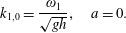
When both gravity and friction act, i.e.
 $\unicode[STIX]{x2202}w/\unicode[STIX]{x2202}x$
is zero, the wavenumber is (cf. Godin (Reference Godin1985))
$\unicode[STIX]{x2202}w/\unicode[STIX]{x2202}x$
is zero, the wavenumber is (cf. Godin (Reference Godin1985))
 $$\begin{eqnarray}k_{1,a}=k_{1,0}\sqrt{1+2\text{i}a},\end{eqnarray}$$
where
 $a$
is measures the strength of friction (cf. (3.8b
))
$a$
is measures the strength of friction (cf. (3.8b
))
 $$\begin{eqnarray}a=\frac{1}{\unicode[STIX]{x03C0}}\frac{c_{d}}{\unicode[STIX]{x1D714}wh_{0}^{2}}\left(f_{2}Q_{0}+\frac{1}{2}f_{1}Q_{hr}\right).\end{eqnarray}$$
The wave travels in the direction into which it is driven by gravity, and friction acts against it. The surface amplitude and discharge are thus affected in the same manner,
 $k_{1,0Q}=k_{1,0z}$
. The friction scale
$k_{1,0Q}=k_{1,0z}$
. The friction scale
 $a$
varies along the river and with the strength of the flow. A Puiseux series expansion with respect to the parameter
$a$
varies along the river and with the strength of the flow. A Puiseux series expansion with respect to the parameter
 $a$
reveals the effect of friction for low river flow
$a$
reveals the effect of friction for low river flow
 $$\begin{eqnarray}k_{1,a}=k_{1,0}(1+\text{i}a),\quad a\rightarrow 0\end{eqnarray}$$
and high river flow, respectively,
 $$\begin{eqnarray}k_{1,a}=k_{1,0}(1+\text{i})\sqrt{a},\quad a\rightarrow \infty .\end{eqnarray}$$
The imaginary and real parts of (3.20a
) and (3.20b
) determine the rates of damping and phase change. Substitution of (3.17) and (3.19) into (3.20a
) reveals that when the flow is low, the friction damps the tide proportionally to the discharge and
 $h_{0}^{-5/2}$
, but it does not influence the phase. When the flow is strong (3.20b
), the friction determines both the rates of damping and phase change. Both rates approach the same value that is proportional to the square root of the discharge and
$h_{0}^{-5/2}$
, but it does not influence the phase. When the flow is strong (3.20b
), the friction determines both the rates of damping and phase change. Both rates approach the same value that is proportional to the square root of the discharge and
 $h_{0}^{-3/2}$
.
$h_{0}^{-3/2}$
.
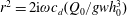
3.6.1 Low river flow
During periods when the river discharge is much smaller than the tidal discharge, the friction coefficients in (3.8a
) and (3.8b
) attain the values
 $f_{1}=3/8$
and
$f_{1}=3/8$
and
 $f_{2}=0$
. This is identical to the approximation by Lorentz (Terra, van de Berg & Maas Reference Terra, van de Berg and Maas2005). In this case,
$f_{2}=0$
. This is identical to the approximation by Lorentz (Terra, van de Berg & Maas Reference Terra, van de Berg and Maas2005). In this case,
 $$\begin{eqnarray}a=\frac{c_{d}}{\unicode[STIX]{x1D714}wh_{0}^{2}}\frac{8}{3\unicode[STIX]{x03C0}}Q_{1}\left(1-4\frac{Q_{0}^{2}}{|Q_{1}|^{2}}\right),\quad |Q_{1}|\gg |Q_{0}|.\end{eqnarray}$$
Damping is thus asymptotically insensitive to river discharge when the tide is strong. River discharge does not add noticeably to the damping as long as
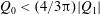 $Q_{0}<(4/3\unicode[STIX]{x03C0})|Q_{1}|$
(figure 5
b). The water depth increases linearly with the river discharge when the river discharge is low, as from (3.3) and (3.8a
), it follows that
$Q_{0}<(4/3\unicode[STIX]{x03C0})|Q_{1}|$
(figure 5
b). The water depth increases linearly with the river discharge when the river discharge is low, as from (3.3) and (3.8a
), it follows that
 $h_{0}\approx h_{0}|_{Q_{0}=0}+x(8/3\unicode[STIX]{x03C0})(c_{d}w/gA_{0}^{3})Q_{hr}Q_{0}$
(figure 5
a). Damping can thus even decrease with the river discharge before a threshold is reached, as the linear increase in water depth can reduce the friction by a larger amount than it is increased by the square of the river discharge, as long as the river flow does not considerably increase the roughness.
$h_{0}\approx h_{0}|_{Q_{0}=0}+x(8/3\unicode[STIX]{x03C0})(c_{d}w/gA_{0}^{3})Q_{hr}Q_{0}$
(figure 5
a). Damping can thus even decrease with the river discharge before a threshold is reached, as the linear increase in water depth can reduce the friction by a larger amount than it is increased by the square of the river discharge, as long as the river flow does not considerably increase the roughness.
Magnitudes of the frequency components of the friction term ((3.8a
)–(3.8c
), bold), depending on the relative strength of river and tidal flow (
 $|Q_{0}|/|Q_{1}|$
), as well as their low flow asymptotes (
$|Q_{0}|/|Q_{1}|$
), as well as their low flow asymptotes (
 $|Q_{0}|/|Q_{1}|\rightarrow 0$
, dash-dotted) and high flow asymptotes (
$|Q_{0}|/|Q_{1}|\rightarrow 0$
, dash-dotted) and high flow asymptotes (
 $|Q_{0}|/|Q_{1}|\rightarrow \infty$
, dashed). Note that the discharge scale is identical to the velocity scale as
$|Q_{0}|/|Q_{1}|\rightarrow \infty$
, dashed). Note that the discharge scale is identical to the velocity scale as
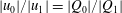 $|u_{0}|/|u_{1}|=|Q_{0}|/|Q_{1}|$
.
$|u_{0}|/|u_{1}|=|Q_{0}|/|Q_{1}|$
.

3.6.2 Strong river flow
When the river discharge is so strong that the flow does not reverse over the tidal cycle, then the friction coefficients (3.8a
) and (3.8b
) obtain the values
 $f_{1}=0$
and
$f_{1}=0$
and
 $f_{2}=\unicode[STIX]{x03C0}$
.
$f_{2}=\unicode[STIX]{x03C0}$
.
 $$\begin{eqnarray}\displaystyle a=\frac{c_{d}}{\unicode[STIX]{x1D714}wh_{0}^{2}}2Q_{0},\quad |Q_{0}|>|Q_{1}|. & & \displaystyle\end{eqnarray}$$
The tide only contributes to the damping rate by modulating the water depth when the river discharge is large, which does not affect the first-order approximation of the damping.
3.7 The effect of width and depth convergence
Width and depth convergence modify the wavenumber by the term
 $\unicode[STIX]{x0394}k_{1}$
. When the cross-section geometry changes smoothly along the river, the term is,
$\unicode[STIX]{x0394}k_{1}$
. When the cross-section geometry changes smoothly along the river, the term is,
 $$\begin{eqnarray}\displaystyle \unicode[STIX]{x0394}k_{1} & = & \displaystyle \frac{1}{4(\text{i}-a)}\left((1+3\text{i}a)\frac{1}{h_{0}}\frac{\unicode[STIX]{x2202}h_{0}}{\unicode[STIX]{x2202}x}+(2+3\text{i}a)\frac{1}{w}\frac{\unicode[STIX]{x2202}w}{\unicode[STIX]{x2202}x}\right),\end{eqnarray}$$
 $$\begin{eqnarray}\displaystyle k_{1z} & = & \displaystyle k_{1,a}+\unicode[STIX]{x0394}k_{1},\end{eqnarray}$$
 $$\begin{eqnarray}\displaystyle k_{1Q} & = & \displaystyle k_{1,a}-\unicode[STIX]{x0394}k_{1}.\end{eqnarray}$$
In contrast to damping, width and depth convergence have the opposite effect on the surface amplitude and the discharge. This corollary of Green’s law (Green Reference Green1838; Jay Reference Jay1991) thus also holds in the presence of friction. The sign of the convergence term also depends on the direction in which the wave travels and in which the cross-section changes. Convergence increases the tidal amplitude when the cross-section becomes narrower and shallower.
In the limit of low friction, the change in wavenumber with the rate of convergence is
 $$\begin{eqnarray}\unicode[STIX]{x0394}k_{1}=-\text{i}\frac{1}{4}\frac{1}{h_{0}}\frac{\unicode[STIX]{x2202}h_{0}}{\unicode[STIX]{x2202}x}-\text{i}\frac{1}{2}\frac{1}{w}\frac{\unicode[STIX]{x2202}w}{\unicode[STIX]{x2202}x},\quad a\rightarrow 0.\end{eqnarray}$$
A relative change in width thus has a larger effect than a relative change in depth of the same magnitude. This is known as Green’s Law (Green Reference Green1838; Jay Reference Jay1991). When friction is strong, the rate of convergence is
 $$\begin{eqnarray}\unicode[STIX]{x0394}k_{1}=-\text{i}\frac{3}{4}\frac{1}{h_{0}}\frac{\unicode[STIX]{x2202}h_{0}}{\unicode[STIX]{x2202}x}-\text{i}\frac{3}{4}\frac{1}{w}\frac{\unicode[STIX]{x2202}w}{\unicode[STIX]{x2202}x},\quad a\rightarrow \infty .\end{eqnarray}$$
Strong friction enhances the effect of convergence, and in contrast to low friction, the relative changes of width and depth have the same effect.
However, the river discharge influences the effect of convergence not only indirectly by increasing friction but also directly, as depth convergence decreases with increasing discharge as
 $\unicode[STIX]{x2202}h_{0}/\unicode[STIX]{x2202}x=\unicode[STIX]{x2202}z_{0}/\unicode[STIX]{x2202}x-\unicode[STIX]{x2202}z_{b}/\unicode[STIX]{x2202}x$
(figure 6
a). The effects of width and depth convergence on the admittance of the tide increase monotonically with the friction and thus with the river and tidal discharge (figure 6
b). However, the depth convergence itself decreases with the river discharge as well, as the upstream water level rises, so that the effect on the admittance has a maximum for intermediate river discharges. Both width and depth convergence primarily affect the amplitude. The rate of phase change is only affected when friction is intermediate.
$\unicode[STIX]{x2202}h_{0}/\unicode[STIX]{x2202}x=\unicode[STIX]{x2202}z_{0}/\unicode[STIX]{x2202}x-\unicode[STIX]{x2202}z_{b}/\unicode[STIX]{x2202}x$
(figure 6
a). The effects of width and depth convergence on the admittance of the tide increase monotonically with the friction and thus with the river and tidal discharge (figure 6
b). However, the depth convergence itself decreases with the river discharge as well, as the upstream water level rises, so that the effect on the admittance has a maximum for intermediate river discharges. Both width and depth convergence primarily affect the amplitude. The rate of phase change is only affected when friction is intermediate.
(a) Relative depth convergence (black) and friction scale (red) at the river mouth depending on the river discharge for infinitesimal waves; (b) effect of depth convergence on the damping rate (black) and rate of phase change (red) depending on the river discharge (solid) or tidal discharge (dashed); damping rate depending on friction and depth convergence (c) as well as width convergence (d) as approximated by (3.23a
), red line shows critical convergence (
 $\text{Im}(k)=0$
), blue and black are asymptotes for high and low friction, respectively.
$\text{Im}(k)=0$
), blue and black are asymptotes for high and low friction, respectively.
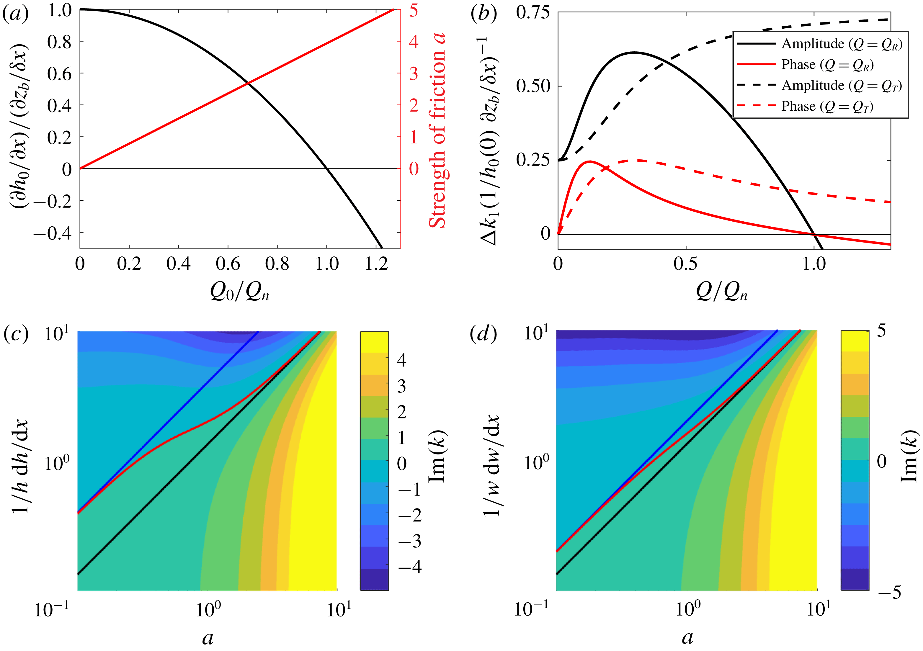
(a) Tidally averaged water level along the river, where the backwater drawdown lengths are indicated by dots; (b) backwater and drawdown length
 $L$
for various states of river flow, defined as the distance to point where water depth deviates no more than 5 %
$L$
for various states of river flow, defined as the distance to point where water depth deviates no more than 5 %
 $(L_{95})$
and approximated by simplified relations.
$(L_{95})$
and approximated by simplified relations.
4 Hydrodynamics of tidal rivers with a sloping bed
This section considers a river with moderate bed slope, where reflection along the channel is small. For illustration, it adopts dimensions that are similar to those of the Kapuas River. At the downstream boundary, the amplitude of the incoming wave is prescribed, and the reflected wave is allowed to pass freely, i.e. without reflection, to the sea. If not otherwise mentioned, the amplitude of this wave is infinitesimal so that the damping is entirely caused by the river flow (3.22). The computational domain ends upstream of the point where the bed reaches sea level, where the tidal wave is allowed to leave the domain without reflection. The examples contrast the propagation of the tide in the presence of backwater effects to that predicted with a conventional model that assumes the tidally averaged water depth to remain constant along the channel and not to change with the river discharge.
4.1 Tidally averaged water level
The tidally averaged water level changes along a river depending on the river discharge. When the river discharge is low, it forms a backwater profile, and depth decreases in the upstream direction (figure 8 black and red). Far upstream, the water surface slope asymptotically approaches the bed slope, so that the tidally averaged water depth remains constant along the river.
There are no analytic solutions to the backwater profile (3.3), with the exception of those of the Bresse type (Vatankhah & Easa Reference Vatankhah and Easa2011), which cannot be integrated into a general solution of the tide because they swap the dependent and independent variables. For the analysis of the river tide, we thus linearize the backwater equation (3.3) and (3.8a ) at the river mouth,
 $$\begin{eqnarray}h_{0}(x)=h_{0}(0)+\left(\left.\frac{\unicode[STIX]{x2202}z_{0}}{\unicode[STIX]{x2202}x}\right|_{0}-\frac{\unicode[STIX]{x2202}z_{b}}{\unicode[STIX]{x2202}x}\right)x+O\left(\left.\frac{\unicode[STIX]{x2202}^{2}z_{0}}{\unicode[STIX]{x2202}x^{2}}\right|_{0}x^{2}\right)=\frac{c_{d}}{g}\frac{Q_{0}|Q_{0}|}{w^{2}h_{0}^{3}},\end{eqnarray}$$
for the reach between the river mouth and the point where the flow becomes approximately uniform
 $(x=|h_{0}(0)-h_{u}|((\unicode[STIX]{x2202}h_{0}/\unicode[STIX]{x2202}x)|_{0})^{-1})$
;
$(x=|h_{0}(0)-h_{u}|((\unicode[STIX]{x2202}h_{0}/\unicode[STIX]{x2202}x)|_{0})^{-1})$
;
 $h_{u}$
is the depth in the reach of uniform flow far upstream.
$h_{u}$
is the depth in the reach of uniform flow far upstream.
When the river is at normal flow
 $(Q=Q_{n})$
, then the water surface slope is identical to the bed slope, and the tidally averaged water depth does not change along the river (blue in figure 7
a). When the river discharge is below normal flow, then the river forms a backwater curve (black, red and green in figure 7
a). When the river discharge is above normal flow, then the water surface forms a drawdown curve so that the depth increases into the upstream direction (orange in figure 7
a). For extremely low river discharge, the point where the flow becomes uniform approaches the point where the bed reaches sea level
$(Q=Q_{n})$
, then the water surface slope is identical to the bed slope, and the tidally averaged water depth does not change along the river (blue in figure 7
a). When the river discharge is below normal flow, then the river forms a backwater curve (black, red and green in figure 7
a). When the river discharge is above normal flow, then the water surface forms a drawdown curve so that the depth increases into the upstream direction (orange in figure 7
a). For extremely low river discharge, the point where the flow becomes uniform approaches the point where the bed reaches sea level
 $x=L_{0}=h_{0}(\unicode[STIX]{x2202}z_{b}/\unicode[STIX]{x2202}x)^{-1}$
. As long as the river is in a state of backwater, this point is located the closer to the river mouth, the higher the discharge is (figure 7
b). As the wavenumber depends on the water depth, the backwater profile strongly influences the admittance of the tide.
$x=L_{0}=h_{0}(\unicode[STIX]{x2202}z_{b}/\unicode[STIX]{x2202}x)^{-1}$
. As long as the river is in a state of backwater, this point is located the closer to the river mouth, the higher the discharge is (figure 7
b). As the wavenumber depends on the water depth, the backwater profile strongly influences the admittance of the tide.
4.2 Admittance along the river
In the case of normal flow, the depth does not converge. The tidal amplitude decreases exponentially along the channel so that the tidal amplitude drops most rapidly near the sea and less rapidly farther upstream (figure 8 b). The wave propagates with constant celerity (figure 9 a). At normal flow, the frictional damping is strong so that the damping rate is proportional to the square root of the river discharge, as given by (3.20a ). This is a well-known relation for the propagation of a tidal wave along a river with constant depth (LeBlond Reference LeBlond1978; Godin Reference Godin1985; Jay Reference Jay1991; Jay & Flinchem Reference Jay and Flinchem1997).
(a) Admittance of the tide for the case where the depth varies along the river (bold) and for the case where the depth remains constant along the river (dashed); inflexion points are indicated by dots, maxima by chevrons; (b) the logarithmic
 $y$
-axis reveals the inversion of the stage–amplitude relation in the asymptotic reach; scenarios as in figure 7(a).
$y$
-axis reveals the inversion of the stage–amplitude relation in the asymptotic reach; scenarios as in figure 7(a).
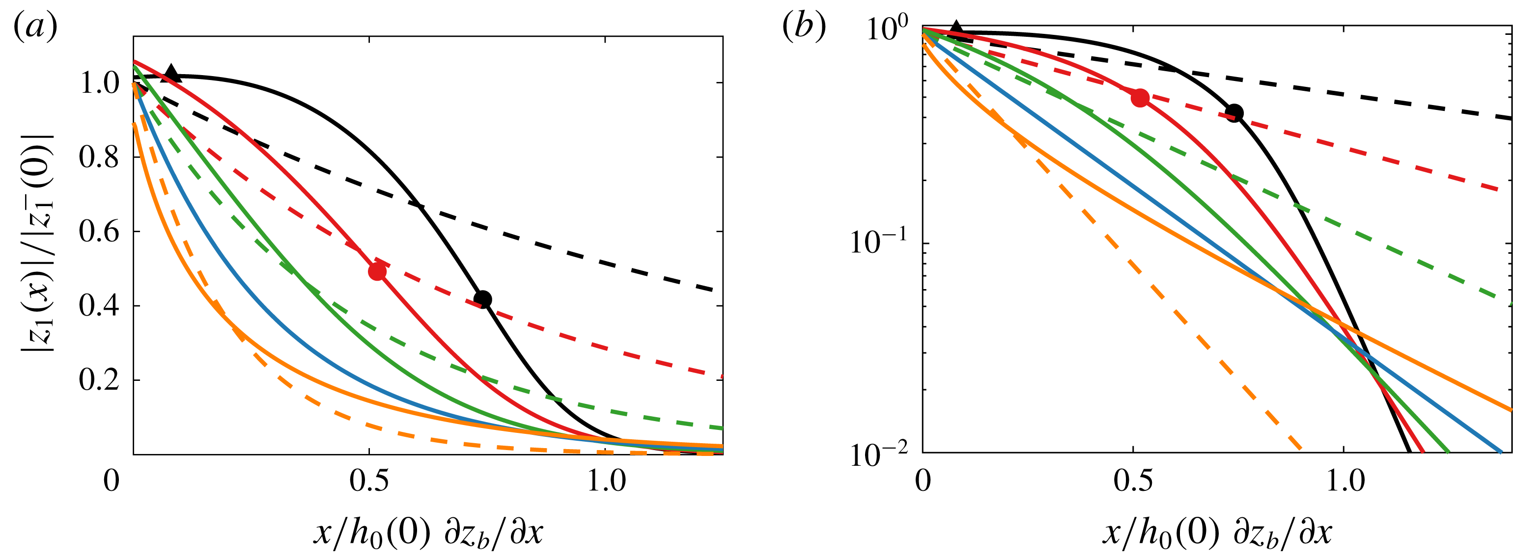
(a) Phase difference between the tidal surface elevation along the river with respect to that at the mouth; (b) phase lag between the tidal velocity and surface level variation along the river. Without backwater effects, the phase difference is zero during low flow, as expected for a progressive wave (black dashed). During high flow, the phase difference is apparently half-way between that of a progressive and a standing wave, although there is no reflection. With the backwater effect, the phase of the tide always appears to be between that of a progressive and a standing wave (solid lines); scenarios as in figure 8.
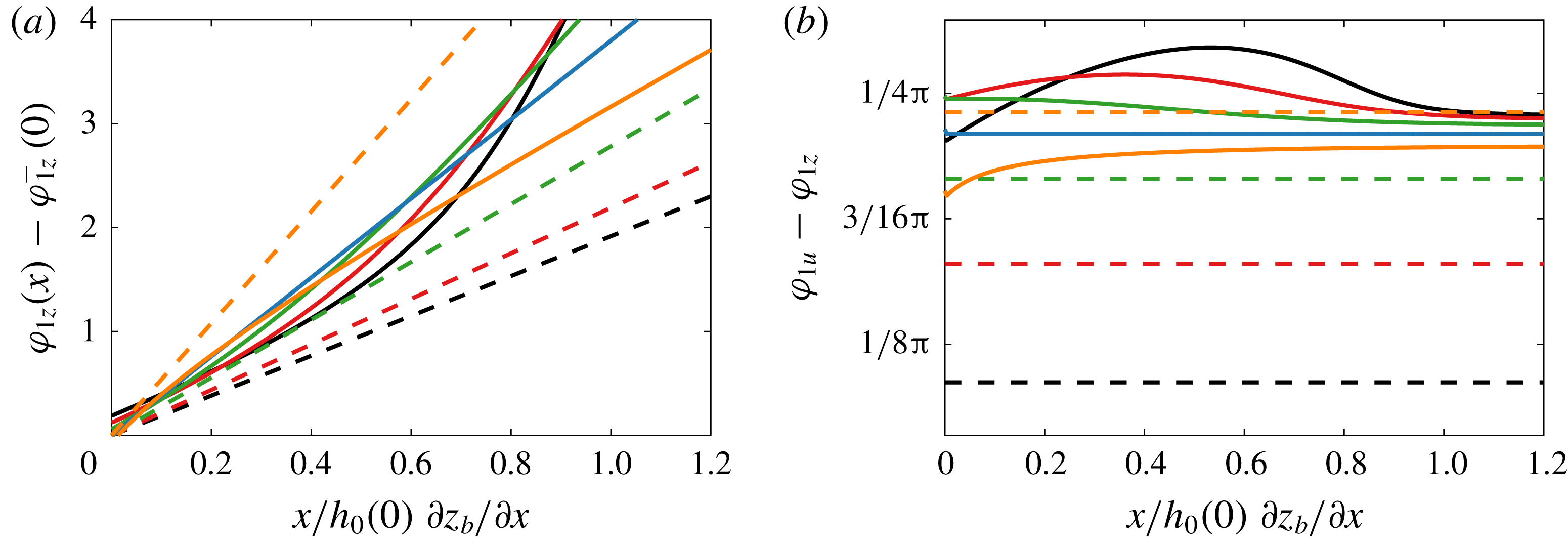
However, when the river is not at normal flow, then the depth changes along the river, and the tide propagates differently compared to the case where the depth remains constant along the river. At low flow (black and red lines in figure 8
a), the tidally averaged water surface forms a backwater profile. The tidal amplitude decreases only slowly near the river mouth, and more rapidly farther upstream (black and red in figure 8
b). The transition is marked by an inflexion point at which
 $\unicode[STIX]{x2202}^{2}|z_{1}|/\unicode[STIX]{x2202}x^{2}=0$
. As (3.11b
) implies
$\unicode[STIX]{x2202}^{2}|z_{1}|/\unicode[STIX]{x2202}x^{2}=0$
. As (3.11b
) implies
 $(1/|z_{1}|)(\unicode[STIX]{x2202}|z_{1}|/\unicode[STIX]{x2202}x)=\text{Im}(k_{1z})$
, this implies
$(1/|z_{1}|)(\unicode[STIX]{x2202}|z_{1}|/\unicode[STIX]{x2202}x)=\text{Im}(k_{1z})$
, this implies
 $$\begin{eqnarray}\frac{\unicode[STIX]{x2202}\text{Im}(k_{1z})}{\unicode[STIX]{x2202}x}-\text{Im}(k_{1z})^{2}=0.\end{eqnarray}$$
The inflexion point is located closer to the sea for higher river discharges, similar to the transition point where the asymptotic flow is reached. For discharges higher than a particular value, the inflexion point is not observed anymore. Only when the river discharge is above this threshold is the tide admitted similarly to the conventional case where the depth is assumed to be constant along the river.
For very low discharges (black), the tidal range even increases in the landward direction to a point where a maximum is reached. The tidal admittance is hypersynchronous. At this point, the imaginary part of the wavenumber is zero,
 $$\begin{eqnarray}\text{Im}(k_{1z})=0.\end{eqnarray}$$
The maximum is located closer to the sea than the inflexion point. This point is related to the concept of critical damping that is used to characterize tidally dominated estuaries (Jay Reference Jay1991). Along such estuaries, width convergence can cancel frictional damping. If the tidally averaged water depth remains constant along an estuary, it can be critically damped along its entire length so that the tidal amplitude neither increases nor decreases, in which case, an estuary is considered to be ‘ideal’. A fundamental difference between tide-dominated estuaries and tidal rivers with a sloping bed is thus that tidal rivers cannot represent ideal estuaries, as the damping can be critical only at one point, and not along the entire tidally influenced reach. The location of this point furthermore depends on the river discharge. Similar to the location of the inflexion point, the maximum is located closer to the sea for higher river discharges and vanishes when the discharge exceeds a certain threshold.
4.3 Damping and convergence rates
The rate of amplitude change along the river is the combined effect of frictional damping and convergence of the width and depth. For large depths, the damping rate is proportional to
 $h_{0}^{-5/2}$
(3.20a
), while depth convergence is proportional to
$h_{0}^{-5/2}$
(3.20a
), while depth convergence is proportional to
 $h_{0}^{-1}$
(3.23a
). At low flow, the river forms a backwater profile, and the depth increases towards the sea. The effects of both the frictional damping and convergence thus decrease towards the sea, but frictional damping decreases more rapidly so that close to the sea, the effect of convergence is larger than that of damping, and the amplitude of waves travelling upstream increases along the downstream part of the tidal river. In this reach, the imaginary part of
$h_{0}^{-1}$
(3.23a
). At low flow, the river forms a backwater profile, and the depth increases towards the sea. The effects of both the frictional damping and convergence thus decrease towards the sea, but frictional damping decreases more rapidly so that close to the sea, the effect of convergence is larger than that of damping, and the amplitude of waves travelling upstream increases along the downstream part of the tidal river. In this reach, the imaginary part of
 $k_{1z}$
is thus positive (figure 10). Conversely, the water depth decreases into the upstream direction towards the point where the bed reaches sea level when the river discharge is low. For small depths, damping is proportional to
$k_{1z}$
is thus positive (figure 10). Conversely, the water depth decreases into the upstream direction towards the point where the bed reaches sea level when the river discharge is low. For small depths, damping is proportional to
 $h_{0}^{-3/2}$
, while convergence is still proportional to
$h_{0}^{-3/2}$
, while convergence is still proportional to
 $h_{0}^{-1}$
. The effects of both damping and convergence thus increase in the upstream direction, but damping increases more rapidly so that eventually frictional damping dominates, and the tidal amplitude is reduced in the upstream part of the tidal river. In this reach, the imaginary part of
$h_{0}^{-1}$
. The effects of both damping and convergence thus increase in the upstream direction, but damping increases more rapidly so that eventually frictional damping dominates, and the tidal amplitude is reduced in the upstream part of the tidal river. In this reach, the imaginary part of
 $k_{1z}$
is thus negative (figure 10). The depth only increases into the upstream direction when the river discharge is very large so that the water surface forms a drawdown curve. In that case, damping is very strong, and convergence has the opposite effect compared to the situation for low flow, so the tidal amplitude rapidly decreases.
$k_{1z}$
is thus negative (figure 10). The depth only increases into the upstream direction when the river discharge is very large so that the water surface forms a drawdown curve. In that case, damping is very strong, and convergence has the opposite effect compared to the situation for low flow, so the tidal amplitude rapidly decreases.
(a) Imaginary (dashed) and real (solid) parts of the wavenumber
 $z_{1}$
, corresponding to the rate of damping and phase change, respectively; critical damping occurs at
$z_{1}$
, corresponding to the rate of damping and phase change, respectively; critical damping occurs at
 $\text{Im}(k_{1z})=0$
. (b) Relative strength of convergence compared to that of gravity and friction (
$\text{Im}(k_{1z})=0$
. (b) Relative strength of convergence compared to that of gravity and friction (
 $\text{Im}(\unicode[STIX]{x0394}k_{1}/k_{1,0})$
, solid) and its approximation by (3.23a
) (dashed), critical damping occurs at
$\text{Im}(\unicode[STIX]{x0394}k_{1}/k_{1,0})$
, solid) and its approximation by (3.23a
) (dashed), critical damping occurs at
 $-1$
; scenarios correspond to those in figure 8.
$-1$
; scenarios correspond to those in figure 8.
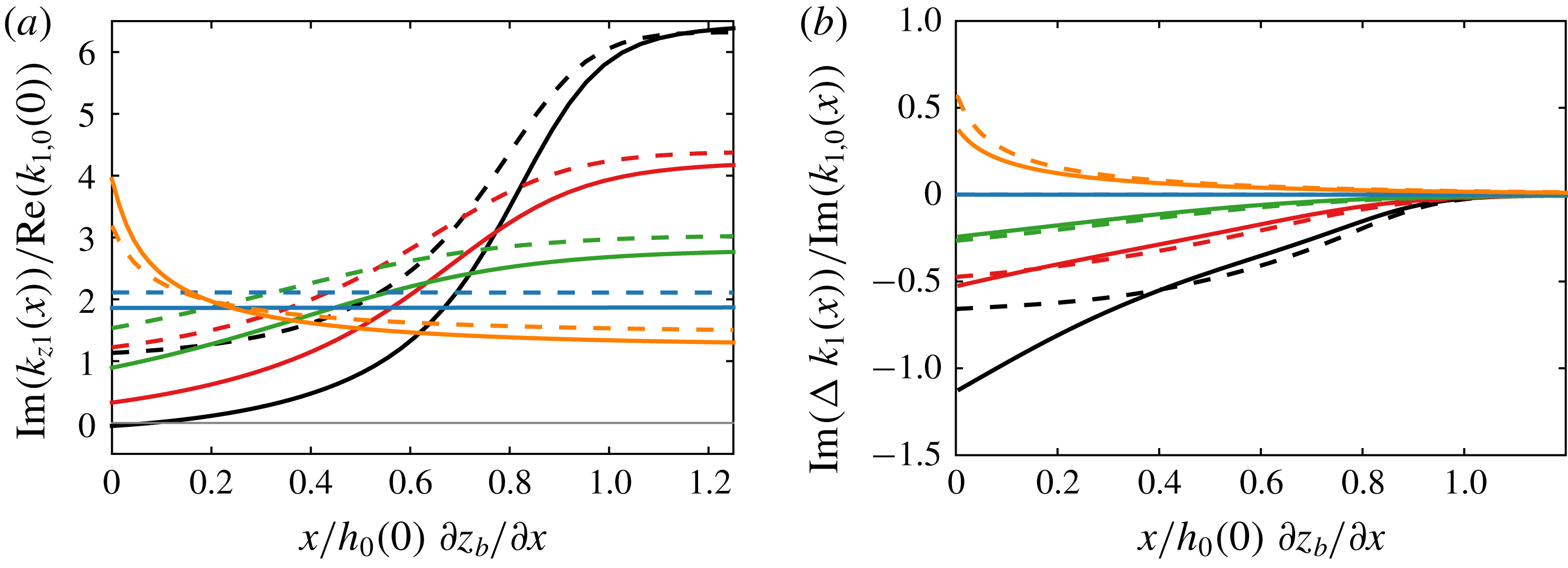
4.4 Asymptotic admittance
The influence of the river discharge on the propagation of the tide in the upstream reach where the flow becomes uniform has been studied by Godin (Reference Godin1985). However, this study does not pay attention to the influence of the river flow on the tidally averaged water depth. When the slope of the river bed is very small, the tidally averaged water depth does not strongly change with the river discharge. In such a case, the damping decreases with the river discharge so that the tide intrudes far upstream during low flow (figure 8 b). However, this is not the case when the slope of the river bed is not small. The admittance is always marginal beyond the point where the bed reaches sea level (figure 8 b). In the asymptotic reach (inset in figure 8), the tidal amplitude even slightly increases with the river discharge. Far upstream, the river flow becomes asymptotically uniform. The ordinary differential equation for the water surface elevation (3.3) simplifies to an algebraic equation referred to as the Chézy formula. The algebraic relation between discharge and surface elevation allows one to eliminate either the river discharge or the water depth from the expression for the wavenumber. Far upstream, damping is strong so that the wavenumber is approximated by (3.20b ),
 $$\begin{eqnarray}\displaystyle k_{1z} & = & \displaystyle -(1-\text{i})\sqrt{\frac{c_{d}\unicode[STIX]{x1D714}Q_{0}}{gwh_{0}^{3}}},\end{eqnarray}$$
 $$\begin{eqnarray}\displaystyle & = & \displaystyle -(1-\text{i})\sqrt{\frac{\unicode[STIX]{x1D714}w}{Q_{0}}\frac{\unicode[STIX]{x2202}z_{b}}{\unicode[STIX]{x2202}x}},\end{eqnarray}$$
 $$\begin{eqnarray}\displaystyle & = & \displaystyle -(1-\text{i})\sqrt[4]{\frac{c_{d}\unicode[STIX]{x1D714}^{2}}{gh_{0}^{3}}\frac{\unicode[STIX]{x2202}z_{b}}{\unicode[STIX]{x2202}x}},\quad x>\left(\frac{1}{h_{0}}\frac{\unicode[STIX]{x2202}z_{b}}{\unicode[STIX]{x2202}x}\right)^{-1}.\end{eqnarray}$$
Tidal admittance for three stations located at a tidal river subject to backwater effects (black) and as predicted by a conventional model that neglects the backwater (red); dashed lines show the admittance of a wave with infinitesimal amplitude, solid lines show the admittance of a wave with finite amplitude; without backwater effects, the admittance decays exponentially; with backwater effects, the admittance decreases hyperbolically along the river.
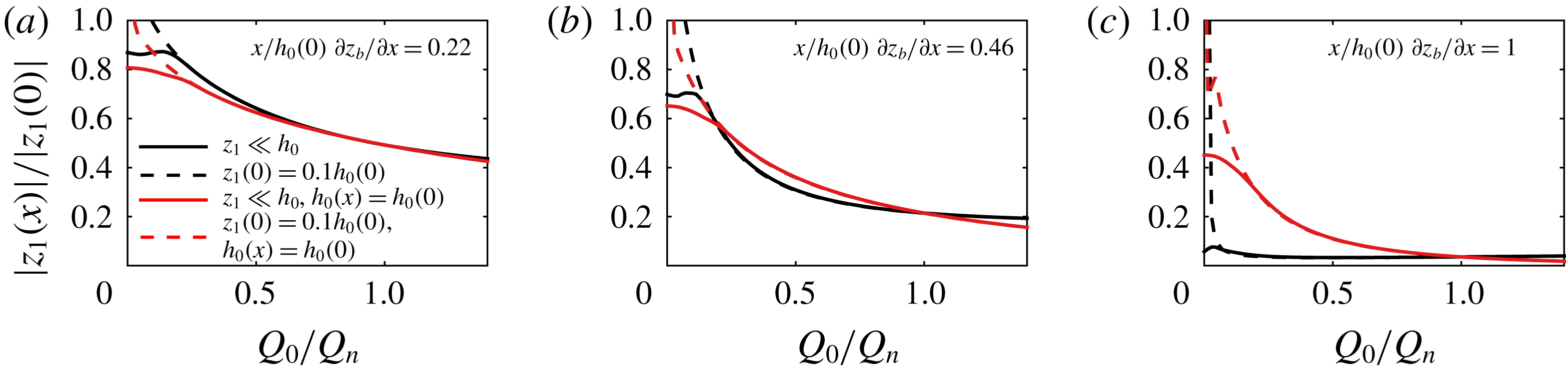
As intuition suggests, the damping becomes the stronger, the larger the slope, due to the higher flow velocity and shallower depth. The expression also shows that damping is indeed asymptotically inversely proportional to the square root of the river discharge so that in the asymptotic reach, the amplitude increases with the river discharge, which is the opposite of what is predicted by conventional models, where the depth remains constant along the river. The expression bears yet another surprise: neither the rate of frictional damping nor that of the phase change asymptotically depend on the drag coefficient for a particular river discharge. The tidal damping along the upstream reach has thus to be calibrated by adjusting other parameters, such as bed slope or channel geometry, rather than the drag coefficient, which is a common parameter for the calibration of hydrodynamic models. Similarly, the rate of damping and phase change are asymptotically independent of the water depth for a particular river discharge.
We point out that upstream propagation of tidal waves is not primarily inhibited by the pull of gravity down the slope, but rather by high friction caused by either the low water depth during low discharges, or by high flow velocities during high discharges. For small discharges, the region where the damping is low extends farther upstream; however, in the asymptotic reach beyond the point where the bed reaches sea level, the tidal amplitude always decreases along the channel. The transition between the reach where friction is low and the asymptotic reach where friction is high is thus more rapid during periods of low river flow than during periods of high river flow.
4.5 At-a-station admittance
The tidal amplitude that is observed at a gauging station depends on the river discharge, in analogy to the admittance of the tide along the river (§ 4.2). Figure 11 shows the admittance of the tide at three stations along a tidal river with a sloping bed in comparison to the admittance that is predicted by a conventional model, which neglects the backwater dynamics and assumes a constant depth along the river.
At a station near the sea, the tidal amplitude is always higher than that predicted by the conventional model (figure 11
a) except at normal flow, when the amplitudes are equal. At a station in the transition reach (figure 11
b), the admittance is higher during low flow and high flow but lower during intermediate river flow. Beyond the point where the river bed reaches sea level (figure 11
c), the admittance is much smaller during low flow and slightly larger during high flow than predicted without bed slope. In general, when the backwater dynamics is neglected, the admittance is predicted to decrease exponentially with the river discharge. The backwater introduces a hyperbolic factor to the admittance due to the gradual change in depth. The tidal amplitude drops less rapidly than predicted by the exponential approximation when the river discharge is low, and more rapidly when the river discharge is high. The hyperbolicity of the tidal admittance can be shown on hand of the propagation of the upstream travelling wave
 $\unicode[STIX]{x2202}z_{1}^{-}/\unicode[STIX]{x2202}x=-\text{i}(k_{1,a}-\unicode[STIX]{x0394}k_{1})z_{1}^{-}$
(3.23c
), when the reflected wave is neglected (
$\unicode[STIX]{x2202}z_{1}^{-}/\unicode[STIX]{x2202}x=-\text{i}(k_{1,a}-\unicode[STIX]{x0394}k_{1})z_{1}^{-}$
(3.23c
), when the reflected wave is neglected (
 $z_{1}\approx z_{1}^{-}$
). The admittance is found by integration
$z_{1}\approx z_{1}^{-}$
). The admittance is found by integration
 $z_{1}(x)=z_{1}(0)\exp (\int _{0}^{x}-\text{i}(k_{1,a}-\unicode[STIX]{x0394}k)\,\text{d}x^{\prime })$
. The linearization of the backwater equation leads to
$z_{1}(x)=z_{1}(0)\exp (\int _{0}^{x}-\text{i}(k_{1,a}-\unicode[STIX]{x0394}k)\,\text{d}x^{\prime })$
. The linearization of the backwater equation leads to
 $\unicode[STIX]{x0394}k_{1}=-\text{i}(p/(1+(1/h_{0}(0))(\unicode[STIX]{x2202}h_{0}/\unicode[STIX]{x2202}x)x))(\unicode[STIX]{x2202}h_{0}/\unicode[STIX]{x2202}x)$
, and an admittance of the form
$\unicode[STIX]{x0394}k_{1}=-\text{i}(p/(1+(1/h_{0}(0))(\unicode[STIX]{x2202}h_{0}/\unicode[STIX]{x2202}x)x))(\unicode[STIX]{x2202}h_{0}/\unicode[STIX]{x2202}x)$
, and an admittance of the form
 $$\begin{eqnarray}\displaystyle z_{1}(x) & {\approx} & \displaystyle \left(\frac{h_{0}(0)}{h_{0}(x)}\right)^{p}\exp \left(\int _{0}^{x}-\text{i}k_{1,a}\,\text{d}x^{\prime }\right)z_{1}(0)\end{eqnarray}$$
 $$\begin{eqnarray}\displaystyle & = & \displaystyle \frac{1}{\displaystyle \left(1+\frac{1}{h_{0}(0)}\frac{\unicode[STIX]{x2202}h}{\unicode[STIX]{x2202}x}x\right)^{p}}\exp \left(\int _{0}^{x}-\text{i}k_{1,a}\,\text{d}x^{\prime }\right)z_{1}(0),\end{eqnarray}$$
 $p$
approaches
$p$
approaches
 $1/4$
for low river flow and
$1/4$
for low river flow and
 $3/4$
for high river flow, according to (3.24) and (3.25).
$3/4$
for high river flow, according to (3.24) and (3.25).4.6 Reflected wave
The approximation (3.16a ) considers only the effect of transmission on the tide but not reflection. However, waves are partially reflected whenever they propagate along a channel where the cross-section changes over a distance that is shorter than its wavelength (Lighthill Reference Lighthill2001). The tide is thus gradually reflected, as the depth diminishes along the backwater affected reach of a tidal river.
When the tidal amplitude is small, the wave reflected back downstream can be approximated by the following double integral,
 $$\begin{eqnarray}Q_{1}^{+}(x)=\int _{x}^{\infty }R^{-}Q_{1}^{-}(x^{\prime })\exp \left(\int _{x^{\prime }}^{x}r^{+}+T^{+}\,\text{d}x^{\prime \prime }\right)\,\text{d}x.\end{eqnarray}$$
The wave that is reflected back downstream is again partially reflected so that the upstream and downstream travelling waves are linearly dependent on each other (Witting Reference Witting1981) ((3.15a
) and (3.15b
)). The step (4.6) can be iterated to decompose the tide into a series that can be interpreted as recursively reflected waves (Wilmer III & Costa Reference Wilmer and Costa2008). The reflected waves decrease rapidly in magnitude, due to the damping and gradual change in depth (
 $|R^{\pm }|\ll 1$
).
$|R^{\pm }|\ll 1$
).
A decomposition of the tidal wave into the incoming and the reflected parts shows that the magnitude of the reflected wave is indeed not entirely negligible (figure 12). The reflected wave increases the amplitude of the total wave. As the reflected wave leaves the river, the amplitude and phase of the tide at the river mouth slightly differ from that of the incoming wave (figure 12, inset). The tide at the river mouth thus depends on the river geometry and river discharge. This is important for the prescription of boundary conditions. It seems natural to specify the surface level
 $z_{s}(t,0)$
at the river mouth, as the astronomical tide can reliably be predicted (Egbert & Erofeeva Reference Egbert and Erofeeva2002). This approach is typically applied in one-dimensional models of tidal rivers that do not include the adjacent sea (Bolla Pittaluga et al.
Reference Bolla Pittaluga, Tambroni, Canestrelli, Slingerland, Lanzoni and Seminara2015). In § 3.6, we apply this to approximate the propagation of the wave. However, this implicitly reduces the amplitude of the tide entering from the sea by the amplitude of the reflected wave and thus violates causality, as it implies that the astronomical tide depended on the estuarine geometry and river discharge. For the numerical computation of the tide in § 4, we therefore only prescribe a value for the incoming wave
$z_{s}(t,0)$
at the river mouth, as the astronomical tide can reliably be predicted (Egbert & Erofeeva Reference Egbert and Erofeeva2002). This approach is typically applied in one-dimensional models of tidal rivers that do not include the adjacent sea (Bolla Pittaluga et al.
Reference Bolla Pittaluga, Tambroni, Canestrelli, Slingerland, Lanzoni and Seminara2015). In § 3.6, we apply this to approximate the propagation of the wave. However, this implicitly reduces the amplitude of the tide entering from the sea by the amplitude of the reflected wave and thus violates causality, as it implies that the astronomical tide depended on the estuarine geometry and river discharge. For the numerical computation of the tide in § 4, we therefore only prescribe a value for the incoming wave
 $\hat{z}_{1}^{-}$
at the seaward boundary, and let the seaward travelling wave
$\hat{z}_{1}^{-}$
at the seaward boundary, and let the seaward travelling wave
 $\hat{z}_{1}^{+}$
pass without reflection. As only one value is specified per frequency component at each boundary, we express it as a linear combination of the incoming and seaward travelling wave, according to (3.14b
). The mean water level at the mouth also varies over a Metonic cycle (Woodworth Reference Woodworth2017) and is due to the river discharge, but these variations are negligible.
$\hat{z}_{1}^{+}$
pass without reflection. As only one value is specified per frequency component at each boundary, we express it as a linear combination of the incoming and seaward travelling wave, according to (3.14b
). The mean water level at the mouth also varies over a Metonic cycle (Woodworth Reference Woodworth2017) and is due to the river discharge, but these variations are negligible.
Conversely, a trivial boundary condition of zero tidal amplitude or discharge causes reflection at the upstream boundary. Reflection at the upstream boundary can be reduced by placing the upstream boundary far from the sea (Godin & Martínez Reference Godin and Martínez1994; Cai et al.
Reference Cai, Savenije and Toffolon2014). We avoid reflection by expressing the upstream boundary condition as a linear combination of the upstream and downstream travelling waves and set only the amplitude of the downstream travelling wave to zero as
 $Q_{1}^{+}=0$
.
$Q_{1}^{+}=0$
.
(a) Admittance of the combined incoming and reflected waves (
 $|z_{1}(x)|/|z_{1}^{-}(0)|$
, solid) and only of the upstream travelling wave (
$|z_{1}(x)|/|z_{1}^{-}(0)|$
, solid) and only of the upstream travelling wave (
 $|z_{1}^{-}(x)|/|z_{1}^{-}(0)|$
, dash-dotted) along the river. (b) amplitude (solid) and phase (dashed) of the combined wave with respect to the incoming wave at the river mouth, depending on the river discharge. Scenarios as in figure 8.
$|z_{1}^{-}(x)|/|z_{1}^{-}(0)|$
, dash-dotted) along the river. (b) amplitude (solid) and phase (dashed) of the combined wave with respect to the incoming wave at the river mouth, depending on the river discharge. Scenarios as in figure 8.

4.7 Tidal propagation where the bed reaches sea level
When the river discharge is very low, the water is shallow near the point where the bed reaches sea level so that the relative change in depth along the river is large. The wave is therefore partially reflected according to (3.15a ). Locally, the reflected wave adds noticeably to the water surface oscillation, but as it travels back, it rapidly decreases in amplitude because the friction is high and the divergence of the cross-sectional area reduces the amplitude of the reflected wave. Near the head of the tidal river, the amplitude of the main tidal species can exceed that of the water depth. The overtide rises low water by changing the shape of the tide so that the river bed does not necessarily fall dry during periods of low river flow.
Without river discharge, the bed dries up beyond the point where the bed reaches sea level so that the tide cannot propagate much farther upstream. The model (3.9a ) forces the tidal amplitude to zero at the point where the bed reaches sea level. The phase of the tide changes at an ever-increasing rate towards the point where the depth reaches zero so that the phase is undefined at this point. This is the case for all waves of zero amplitude and is not an artefact of the model. In practice, a short reach upstream of the head of the tidal river can periodically flood and dry over the tidal cycle. The flow furthermore concentrates near the thalweg, and shallow parts of the cross-section are periodically flooded. A model that has a bed that is not flat across the river can better predict how the tide propagates near the head. However, the solution is sensitive to unevenness of the river bed, to seasonal variation of the sea level as well as to the residual river flow. Wetting and drying of the entire cross-section is also beyond the scope of the shallow-water equations (3.2a ) and (3.2b ), as those require the depth to be non-zero at all time. In any case, the tide does not propagate far beyond the point where the bed reaches sea level during periods without river flow, as it rapidly decays due to the shallow depth as well as storage on the higher parts of the bed that are periodically flooded. The case of the wave vanishing when running up the slope thus contrasts with the case where the wave runs against a wall, where the surface amplitude obtains a maximum, as well as the case with a wave propagation along a channel with a horizontal bed, where the wave propagates incessantly, without ever entirely decaying to zero. A minimum base flow ensures that the bed of the Kapuas never falls entirely dry. However, bars and dunes emerge during low flow beyond the point where the bed reaches sea level, which is slightly upstream of the city of Sanggau.
Magnitudes of tidal discharge (a) and tidal velocity (b), along a tidal river with a sloping bed (solid), and constant depth (dashed); river discharge indicated by dash-dotted line in (a); scenarios as in figure 8.

4.8 Tidal discharge
The tidal discharge decreases with increasing river discharge (figure 13 a). It diminishes gradually along the river so that no extrema or inflexion points occur.
As long as the river discharge is low, the tidally averaged water surface forms a backwater profile, and the tidal discharge at the river mouth decreases at a higher rate than that predicted without a sloping bed.
The most upstream point of flow reversal is located closer to the sea, compared to the conventional model. Similar to the tidal water surface amplitude, the tidal discharge amplitude is marginal beyond the point where the river bed reaches sea level. The higher rate at which the discharge is reduced is caused by depth convergence, which, recalling (3.23a ), has an effect on the discharge that is opposite to the effect on the tidal surface level amplitude. The lower initial discharge at the river mouth is also a direct consequence of depth convergence. Recalling the continuity (3.2a ), the tidal discharge of the main species is
 $$\begin{eqnarray}Q_{1}=\text{i}w\frac{\unicode[STIX]{x1D714}}{k_{1Q}}z_{1},\end{eqnarray}$$
which can be directly evaluated at the river mouth in combination with the approximate wavenumber (3.16a
). The tidal discharge at the river mouth is thus smaller because it is inversely proportional to the wavenumber
 $k_{1Q}$
, which itself is larger in magnitude, due to depth convergence.
$k_{1Q}$
, which itself is larger in magnitude, due to depth convergence.
4.9 Tidal velocity
The cross-section averaged flow velocity is directly proportional to the discharge
 $u=1/A_{0}Q$
and can thus also be explicitly evaluated at the river mouth. The tidal velocity amplitude decreases with the river discharge. However, the magnitude of the tidal velocity amplitude decreases along the river at a lower rate than the tidal discharge when the river is below normal flow, which follows from the chain rule,
$u=1/A_{0}Q$
and can thus also be explicitly evaluated at the river mouth. The tidal velocity amplitude decreases with the river discharge. However, the magnitude of the tidal velocity amplitude decreases along the river at a lower rate than the tidal discharge when the river is below normal flow, which follows from the chain rule,
 $$\begin{eqnarray}k_{1u}=-\text{i}\frac{1}{u_{1}}\frac{\unicode[STIX]{x2202}u_{1}}{\unicode[STIX]{x2202}x}=\text{i}\frac{1}{h_{0}}\frac{\unicode[STIX]{x2202}h_{0}}{\unicode[STIX]{x2202}x}+\text{i}\frac{1}{w}\frac{\unicode[STIX]{x2202}w}{\unicode[STIX]{x2202}x}+k_{1Q}.\end{eqnarray}$$
Width and depth convergence increase the magnitude of the velocity compared to the discharge, similar to the surface elevation amplitude, but the phase is similar to that of the discharge. An inflexion point marks the transition to the upstream reach of the tidal river, where the tidal velocity amplitude is rapidly reduced. The inflexion point of the velocity is located the closer to the river mouth, the higher the river discharge (figure 13), similarly to the inflection point of the tidal surface elevation amplitude. Overall, the magnitude of the tidal velocity amplitude decreases at a slightly higher rate than the magnitude of the tidal surface elevation, and the inflexion point of the velocity is located closer to the sea.
When the river flow is very low, the tidal velocity amplitudes are higher than that predicted by a conventional model along the downstream reach of a tidal river. The value is furthermore lower for intermediate discharges compared to that predicted without a sloping bed. The tidal excursion length near the sea is similar but decreases more rapidly towards upstream than that predicted without bed slope (not shown). As the salinity intrusion depends on the tidal excursion (Savenije Reference Savenije2012), this implies that a sloping bed shortens the distance that salinity intrudes up river, as long as the slope does not strongly change the mixing.
4.10 Phase lag
The damping of the tide is related to the phase lag
 $\unicode[STIX]{x0394}\unicode[STIX]{x1D711}_{1}=\arg (u_{1})-\arg (z_{1})$
between the oscillation of the water surface and velocity. When the tidally averaged water depth does not change along the river, then the damping rate and phase lag are directly proportional as long as the damping is low, which follows from (3.20a
)
$\unicode[STIX]{x0394}\unicode[STIX]{x1D711}_{1}=\arg (u_{1})-\arg (z_{1})$
between the oscillation of the water surface and velocity. When the tidally averaged water depth does not change along the river, then the damping rate and phase lag are directly proportional as long as the damping is low, which follows from (3.20a
)
 $$\begin{eqnarray}\unicode[STIX]{x0394}\unicode[STIX]{x1D711}_{1}=\arctan (a)\approx a,\quad a<1,\end{eqnarray}$$
which coincides with the definition of Savenije (Reference Savenije2012) for the case of non-converging estuaries. For weak damping (
 $a\rightarrow 0$
), the velocity is in phase with the surface elevation, as expected for a progressive wave. For strong damping
$a\rightarrow 0$
), the velocity is in phase with the surface elevation, as expected for a progressive wave. For strong damping
 $(a\gg 1)$
, the phase lag is close to
$(a\gg 1)$
, the phase lag is close to
 $\unicode[STIX]{x03C0}/4$
, according to (3.20b
). The phase lag is apparently in between that of a progressive and a standing wave, although the wave is not reflected.
$\unicode[STIX]{x03C0}/4$
, according to (3.20b
). The phase lag is apparently in between that of a progressive and a standing wave, although the wave is not reflected.
Along rivers with a sloping bed, the tidal amplitudes of the surface level and discharge change at different rates so that damping is no longer proportional to the phase lag (figure 9
b). This is the case because friction is always strong in the upstream part of the tidal river and because a part of the wave is reflected gradually along the backwater affected reach. As a consequence, the phase lag is close to
 $\unicode[STIX]{x03C0}/4$
independent of the river flow and can even exceed
$\unicode[STIX]{x03C0}/4$
independent of the river flow and can even exceed
 $\unicode[STIX]{x03C0}/4$
in the upstream part of the tidal river. The phase lag thus does not linearly increase with the river discharge along the backwater affected reach. In the asymptotic flow reach, the phase lag even decreases with the river discharge, opposite to what occurs in a river with a horizontal bed.
$\unicode[STIX]{x03C0}/4$
in the upstream part of the tidal river. The phase lag thus does not linearly increase with the river discharge along the backwater affected reach. In the asymptotic flow reach, the phase lag even decreases with the river discharge, opposite to what occurs in a river with a horizontal bed.
(a) At a station, water level variation over a tidal cycle for
 $z_{1}(0)=0.1h_{0}(0)$
; (b) along river amplitude of the even overtide; (c) along river subtidal water level set-up; solid lines show the tide in a backwater affected river, and dashed lines show the prediction of the tide when the backwater is neglected; scenarios as in figure 8.
$z_{1}(0)=0.1h_{0}(0)$
; (b) along river amplitude of the even overtide; (c) along river subtidal water level set-up; solid lines show the tide in a backwater affected river, and dashed lines show the prediction of the tide when the backwater is neglected; scenarios as in figure 8.

4.11 Overtide generation
Friction not only damps the tide but also generates higher frequency components, referred to as the overtide. The principal overtide advances high water and delays low water so that the tidal wave changes its shape while travelling upstream (figure 14 a). The river discharge forces the principal overtide with twice the frequency and an amplitude proportional to the square of the main tidal species, which is evident from the frequency decomposition of the friction (3.8a ).
When the tidally averaged width and water depth do not change along the river, then the even overtide is determined by the equation
 $$\begin{eqnarray}\frac{\unicode[STIX]{x2202}^{2}Q_{2}}{\unicode[STIX]{x2202}x^{2}}-2\text{i}r_{2}Q_{2}=-\text{i}\frac{r_{1}^{2}}{w}\frac{Q_{1}^{2}}{Q_{0}},\end{eqnarray}$$
which is a simplification of (3.4) and (3.8c
) for the limit that the river flow is much stronger than the tidal flow. The wavenumber
 $k_{1}$
is given by (3.18);
$k_{1}$
is given by (3.18);
 $r_{1}$
is its imaginary part, and
$r_{1}$
is its imaginary part, and
 $k_{2}=\sqrt{2}k_{1}$
as well as
$k_{2}=\sqrt{2}k_{1}$
as well as
 $r_{2}=\sqrt{2}r_{1}$
. This gives the amplitude of the overtide as
$r_{2}=\sqrt{2}r_{1}$
. This gives the amplitude of the overtide as
 $$\begin{eqnarray}z_{2}=\frac{\unicode[STIX]{x1D714}_{1}w}{8r_{1}Q_{0}}z_{1}(0)^{2}(\exp (-2\text{i}k_{1}x)-\exp (-1\text{i}k_{2}x)),\end{eqnarray}$$
for the case when the amplitude of the overtide is zero at the river mouth. Note that even if the surface elevation amplitude of the overtide is zero at the river mouth, the amplitude of the velocity is not, which is due to continuity (4.7). Equation (4.11) is the sum of two decaying exponentials, which add to zero at the river mouth. Near the mouth the principal overtide increases by 0.6 times the rate of that at which the amplitude of the main tidal species decreases, and far upstream, it decreases by 1.4 times the rate of that of the main tidal species.
In a river with a sloping bed, the principal overtide increases near the sea, similar to the case when the tidally averaged water depth remains constant. However, in the upstream part of the tidal river, the tide is damped more rapidly when the bed is sloping. Similar to the main tidal species, the amplitude becomes marginal beyond the point where the bed level reaches sea level (figure 14 b).
4.12 Water level set-up
The tidal flow raises the tidally averaged water level by increasing friction (3.3). The water level, therefore, oscillates with the tidal range over the spring-neap cycle. Such subtidal harmonics have been described by LeBlond (Reference LeBlond1979), Kukulka & Jay (Reference Kukulka and Jay2003a
), Buschman et al. (Reference Buschman, Hoitink, van der Vegt and Hoekstra2009) and Sassi & Hoitink (Reference Sassi and Hoitink2013). The water level set-up
 $z_{0}^{\prime }$
caused by the tide with respect to the water depth
$z_{0}^{\prime }$
caused by the tide with respect to the water depth
 $h_{0}^{\prime }$
that is only due to river flow can be approximated by a perturbation expansion of the backwater equation (3.3). For dominant river flow, this is done by substituting
$h_{0}^{\prime }$
that is only due to river flow can be approximated by a perturbation expansion of the backwater equation (3.3). For dominant river flow, this is done by substituting
 $h_{0}^{\prime }+z_{0}^{\prime }$
for
$h_{0}^{\prime }+z_{0}^{\prime }$
for
 $h_{0}$
, expanding the equations as a series in
$h_{0}$
, expanding the equations as a series in
 $z_{0}^{\prime }$
and keeping only the terms of largest magnitude,
$z_{0}^{\prime }$
and keeping only the terms of largest magnitude,
 $$\begin{eqnarray}\frac{\unicode[STIX]{x2202}z_{0}^{\prime }}{\unicode[STIX]{x2202}x}=\frac{c_{d}}{gw^{2}h_{0}^{4}}\left(\frac{1}{2}|Q_{1}|^{2}h_{0}-3Q_{0}^{2}z_{0}^{\prime }\right).\end{eqnarray}$$
The first term generates and the second term damps the water level set-up. For a river at normal flow, where the tidally averaged water depth remains constant along the channel, the water level set-up is,
 $$\begin{eqnarray}\displaystyle & \displaystyle z_{0}^{\prime }=\frac{h_{0}}{6}\frac{r_{0}}{r_{0}-r_{1}}\frac{|Q_{1}(0)|^{2}}{|Q_{0}|^{2}}(\exp (-2r_{0}x)-\exp (-2r_{1}x)), & \displaystyle\end{eqnarray}$$
 $$\begin{eqnarray}\displaystyle & \displaystyle r_{0}=\frac{1}{2}\frac{c_{d}Q_{0}^{2}}{gw^{2}h_{0}^{4}}. & \displaystyle\end{eqnarray}$$
A similar relation has recently been published by Tolkova (Reference Tolkova2018). Here,
 $r_{1}=\text{Im}(k_{1,a})$
is the damping rate of the main tidal species as given by (3.18), and
$r_{1}=\text{Im}(k_{1,a})$
is the damping rate of the main tidal species as given by (3.18), and
 $r_{0}$
is the damping rate of the mean water level set-up;
$r_{0}$
is the damping rate of the mean water level set-up;
 $Q_{1}(0)$
is the discharge at the river mouth as given by (4.7). The water level set-up is the difference of two decaying exponentials, which are zero at the river mouth. The water level set-up rises along the river twice as rapidly as the main tidal species is damped but thereafter, decays at a lower rate than the main tidal species, because
$Q_{1}(0)$
is the discharge at the river mouth as given by (4.7). The water level set-up is the difference of two decaying exponentials, which are zero at the river mouth. The water level set-up rises along the river twice as rapidly as the main tidal species is damped but thereafter, decays at a lower rate than the main tidal species, because
 $r_{0}\ll r_{1}$
(figure 14
c).
$r_{0}\ll r_{1}$
(figure 14
c).
In rivers with a sloping bed, the tidally averaged water level set-up is always marginal beyond the point where the bed reaches sea level (figure 14 c). The water level set-up has thus a pronounced local maximum. This maximum is lower and closer to the river mouth for higher river discharge. The rapid reduction of the water level set-up in the upstream part of the tidal river is, as the reduction of the tidal amplitude, caused by the variation of the water depth with the river discharge.
Far upstream, where the flow becomes asymptotically uniform, the damping rate can be expressed as a function of the water level only, similar to that of the main tidal species (4.4c )
 $$\begin{eqnarray}r_{0}=-\frac{1}{2}\frac{1}{h_{0}}\frac{\unicode[STIX]{x2202}z_{b}}{\unicode[STIX]{x2202}x},\quad x\rightarrow \infty .\end{eqnarray}$$
This rate is higher than that of the main tidal species (4.4c ), and similar to it, decreases with the river discharge.
The amplitude of the principal overtide and the subtidal water level set-up change along the channel in a similar manner because they are both forced by the part of the friction term that is proportional to
 $Q_{1}^{2}$
; however, the overtide damps out more rapidly. When the main tidal species is diurnal, as in the Kapuas, then the overtide is superimposed on the semi-diurnal tide that enters the river from the sea so that the semi-diurnal tide along the river strongly depends on the river flow.
$Q_{1}^{2}$
; however, the overtide damps out more rapidly. When the main tidal species is diurnal, as in the Kapuas, then the overtide is superimposed on the semi-diurnal tide that enters the river from the sea so that the semi-diurnal tide along the river strongly depends on the river flow.
5 Discussion
In a channel with a horizontal bed, the tide would intrude thousands of kilometres upstream during low river flow (Godin & Martínez Reference Godin and Martínez1994; Cai et al. Reference Cai, Savenije and Toffolon2014). The limit of tidal intrusion observed in natural rivers is often related to dams or cataracts (Parker Reference Parker2007; Jay et al. Reference Jay, Leffler, Diefenderfer and Borde2015). However, a sloping bed sufficiently explains the extinction of the tide and no physical obstacle is required.
Even when the bed is horizontal, the water depth varies with the river discharge (Cai et al. Reference Cai, Savenije, Jiang, Zhao and Yang2016). Without a sloping bed, the water surface elevation forms a drawdown curve even during low flow, and the river does not asymptotically approach uniform flow. The assumption of a horizontal bed is thus not realistic. With a sloping bed, the water surface forms a backwater profile during low flow so that the tide propagates distinctly differently. This is important because the tide is strongest when the river discharge is low. Tidal rivers can be expected to be more often in a state of backwater than subject to drawdown, as their morphology is shaped by high flows, which occur infrequently.
Near the river mouth, the tidal flow is strong, which is relevant in the context of sediment transport and the intrusion of salinity. The tidal influence is particularly large in the region where the flow reverses. At some point along the river, the amplitude of the tidal discharge approximately equals the river discharge. The tidal discharge decreases more rapidly along the river for a higher bed slope, which moves the most upstream point of flow reversal, and thus the fluvial–tidal transition, closer to the sea (§ 4.8). This more rapid transition between the tidally influenced and the exclusively fluvial reach also leaves traces in the morphology. In the Kapuas, for example, the fluvial–tidal transition is marked by a rapid reduction in bed material grain size as well as of the bed form height (Kästner et al. Reference Kästner, Hoitink, Vermeulen, Geertsema and Ningsih2017).
In rivers with a horizontal bed, the water level set-up induced by the tide reaches far upstream, where the amplitude of the main tidal species has long become insignificant (Hoitink & Jay Reference Hoitink and Jay2016). The point where the tidally averaged water level set-up elevates the spring tidal range more than the tidal range difference between the spring tide and the neap tide is considered to be the upstream end of the fluvial–tidal transition (Jay et al. Reference Jay, Leffler, Diefenderfer and Borde2015). At this point, the lowest low water occurs at neap tide, not at spring tide anymore. In rivers with a sloping bed, the water level set-up becomes marginally small beyond the point where the bed reaches sea level; thus, it does not reach far upstream (§ 4.12).
One important effect of a sloping bed is that the tidal amplitude rapidly decreases beyond the point where the bed level reaches sea level under all flow conditions. This effect limits the extent to which sea level rise poses a risk to upstream areas. A rise in sea level merely shifts the head of tides farther upstream, leaving the reaches beyond the point where the bed reaches the higher sea level unaffected. Surprisingly, the bed slope has so far not been considered to be a major factor that influences the resilience of estuaries and rivers with respect to sea level rise (Prandle & Lane Reference Prandle and Lane2015).
However, the land adjoined to those reaches can be at risk of overland flooding during storm surges in gently sloping coastal lowlands (Frazier et al. Reference Frazier, Wood, Yarnal and Bauer2010). In our idealized analysis, we keep the drag coefficients constant. In practice, the bed roughness varies with the tidal and river discharge in a complex manner (van Rijn Reference van Rijn1984). As the idealized model still reproduces the observations of the river tide in the Kapuas, we conclude that the variation of roughness is less important than that of the water depth and that therefore, the bed slope is a more important factor to consider than varying roughness. This notwithstanding, changes in roughness can be relevant for operational flood forecasting (Reef et al. Reference Reef, Lipari, Roos and Hulscher2018).
The backwater dynamics explains the tidal admittance in the Kapuas, where the tidal amplitude does not decay exponentially during low flow as predicted by conventional models of river tides. Waves joining from the subordinary distributaries may partially increase the tidal amplitude in the main channel, the Kapuas Besar. However, bifurcations only locally affect the tidal amplitude and thus cannot explain the observed gradual deviation from an exponential decay. A small increase of the amplitude can be observed at the bifurcation of the largest side distributary, the Kapuas Kecil. This observation is in line with the theory of transmission and reflection at bifurcations (Lighthill Reference Lighthill2001), according to which a small channel that joins a larger one only exerts a small influence on the latter. In turn, the Kapuas Besar strongly forces the subordinate distributaries. Backwater dynamics is thus the most likely cause for the observed low flow admittance in the Kapuas River.
The estuarine geometry strongly influences how the tide propagates (Friedrichs Reference Friedrichs and Valle-Levinson2010). We analyse the tidal propagation along a river with idealized geometry, as this reveals the general effects of a sloping bed and allows for a mathematical explanation. Our findings are relevant for rivers that do not converge in width and where depth converges approximately linearly during low flow (§ 4.1). This is different from tide-dominated estuaries, where the width converges exponentially and where the tidally averaged water level varies only slightly between the seasons (Savenije et al. Reference Savenije, Toffolon, Haas and Veling2008; van Rijn Reference van Rijn2011; Garel & Cai Reference Garel and Cai2018). The bed slope in our models is constant, whereas on the basin scale, the slope decreases along rivers in the downstream direction (Richards Reference Richards1982). A constant slope approach can be justified based on the results of Seminara et al. (Reference Seminara, Pittaluga, Tambroni, Rodi and Uhlmann2012), who showed the bed slope is approximately constant along tidal rivers in morphological equilibrium.
6 Conclusion
Our observations from the Kapuas River show that the tide propagates distinctly differently during low flow than that expected from idealized models that ignore the bed slope. Rather than decreasing exponentially in amplitude and intruding far upstream, the tide remains isosynchronous near the sea, and then rapidly diminishes where the bed reaches sea level. Conventionally, tidal rivers are conceptualized as non-converging channels with a horizontal bed, where the tidally averaged width and depth neither change along the channel nor over time. However, the tidally averaged water depth remains only constant near the sea, and the bed rises along the river. Farther upstream, the depth thus varies with the river discharge so that the water surface forms a backwater profile during low flow. The backwater effect is relevant because tides are strongest during low flow. We extend the idealized model of tidal rivers to include the effects of backwater. Our idealized model shows that the backwater profile considerably influences how the tide propagates during low flow. The principal effect is a larger than expected tidal range near the sea, due to convergence of the depth, as well as a lower than expected tidal range far upstream, due to lower depth and higher friction. Tidal intrusion is effectively limited to the point where the bed reaches sea level, which also applies to the overtide and the tidally averaged water level set-up. Our extended model not only explains the observed tidal dynamics in the Kapuas River but resembles, in general, a more comprehensive model of river tides, since variation of the river discharge and a sloping bed are common to all rivers.
Acknowledgements
This research was supported by the Royal Netherlands Academy of Arts and Sciences (KNAW) project SPIN3-JRP-29. The authors thank T. J. Geertsema (Wageningen University) and M. Pramulya (Tanjungpura University Pontianak) for supporting the project in the field as well as P. Hazenberg (Wageningen University) for technical support. Bulk raw data are available from the first author (Wageningen University, Hydrology and Quantitative Water Management Group, P.O. box 47, 6700 AA Wageningen, The Netherlands, karl.kastner@wur.nl). E.D. is an honorary Research associate with the Belgian Fund for Scientific Research (F.R.S. – FNRS).
Appendix A. Transformation the shallow water into the wave equation
The cross-sectionally averaged shallow-water equations (3.2a ) and (3.2b ) rely on the following assumptions
(i) hydrostatic flow;
(ii) rectangular cross-section without tidal flats;
(iii) straight channel;
(iv) negligible side inflow;
(v) negligible variation of velocity within the cross-section (unit Boussinesq coefficient);
(vi) negligible Coriolis force;
(vii) negligible density gradients.
The following steps transform the shallow-water equation into the wave equation (3.4):
(i) rewrite the momentum equation (3.2b ) in its reduced form:
(A 1) $$\begin{eqnarray}\frac{\unicode[STIX]{x2202}Q}{\unicode[STIX]{x2202}t}+\frac{\unicode[STIX]{x2202}}{\unicode[STIX]{x2202}x}\left(\frac{Q}{A^{2}}\right)+gA\frac{\unicode[STIX]{x2202}z_{s}}{\unicode[STIX]{x2202}x}+c_{d}\frac{|Q|Q}{AR_{h}}=0;\end{eqnarray}$$
(ii) ignore advective acceleration
$((\unicode[STIX]{x2202}/\unicode[STIX]{x2202}x)(Q/A)\ll \unicode[STIX]{x2202}Q/\unicode[STIX]{x2202}t)$
;(iii) divide the momentum equation by
$A$
;(iv) approximate the hydraulic radius for a wide channel
$R_{h}\rightarrow h$
;(v)
$A\rightarrow wh$
;(vi) expand
$1/h^{p}$
as a truncated Taylor series (
$1/h^{p}\rightarrow 1/h_{0}^{p}$
);(vii)
$h\rightarrow h_{0}+z$
, where
$h_{0}=z_{0}-z_{b}$
;(viii) differentiate the continuity equation with respect to
$x$
;(ix) divide the continuity equation by
$w$
;(x) differentiate the momentum equation with respect to
$t$
;(xi) divide the momentum equation by
$g$
;(xii) eliminate
$z$
by subtracting the continuity from the momentum equation.


The result is the wave equation (3.4).
Appendix B. Friction term
This section derives the frequency components (3.8a
)–(3.8b
) of the Chebyshev approximation of the signed square
 $|Q|Q$
of the friction term (3.6). The products and powers of complex exponentials are reduced by the following identities,
$|Q|Q$
of the friction term (3.6). The products and powers of complex exponentials are reduced by the following identities,
 $$\begin{eqnarray}\displaystyle \text{Re}\{c_{1}\text{e}^{\text{i}\unicode[STIX]{x1D714}_{1}t}\}\text{Re}\{c_{2}\text{e}^{\text{i}\unicode[STIX]{x1D714}_{2}t}\} & = & \displaystyle {\textstyle \frac{1}{2}}\text{Re}\{c_{1}c_{2}\text{e}^{\text{i}(\unicode[STIX]{x1D714}_{1}+\unicode[STIX]{x1D714}_{2})t}\}\nonumber\\ \displaystyle & & \displaystyle +\,{\textstyle \frac{1}{2}}\text{Re}\{c_{2}c_{1}^{\ast }\text{e}^{\text{i}(\unicode[STIX]{x1D714}_{2}-\unicode[STIX]{x1D714}_{1})t}\},\end{eqnarray}$$
 $$\begin{eqnarray}\displaystyle \text{Im}(c) & = & \displaystyle \text{Re}\{-\text{i}c\},\end{eqnarray}$$
 $$\begin{eqnarray}\displaystyle cc^{\ast } & = & \displaystyle |c|^{2},\end{eqnarray}$$
 $^{\ast }$
denotes the complex conjugate. The expansion of the discharge
$^{\ast }$
denotes the complex conjugate. The expansion of the discharge
 $Q$
up to the two leading non-zero frequency components (
$Q$
up to the two leading non-zero frequency components (
 $\unicode[STIX]{x1D714}_{j}=j\unicode[STIX]{x1D714}_{1}$
) yields
$\unicode[STIX]{x1D714}_{j}=j\unicode[STIX]{x1D714}_{1}$
) yields 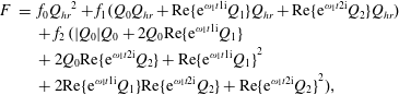 $$\begin{eqnarray}\displaystyle F & = & \displaystyle f_{0}{Q_{hr}}^{2}+f_{1}(Q_{0}Q_{hr}+\text{Re}\{\text{e}^{\unicode[STIX]{x1D714}_{1}t1\text{i}}Q_{1}\}Q_{hr}+\text{Re}\{\text{e}^{\unicode[STIX]{x1D714}_{1}t2\text{i}}Q_{2}\}Q_{hr})\nonumber\\ \displaystyle & & \displaystyle +\,f_{2} (\!|Q_{0}|Q_{0}+2Q_{0}\text{Re}\{\text{e}^{\unicode[STIX]{x1D714}_{1}t1\text{i}}Q_{1}\}\nonumber\\ \displaystyle & & \displaystyle +\,2Q_{0}\text{Re}\{\text{e}^{\unicode[STIX]{x1D714}_{1}t2\text{i}}Q_{2}\}+\text{Re}\{\text{e}^{\unicode[STIX]{x1D714}_{1}t1\text{i}}Q_{1}\}^{2}\nonumber\\ \displaystyle & & \displaystyle +\,2\text{Re}\{\text{e}^{\unicode[STIX]{x1D714}_{1}t1\text{i}}Q_{1}\}\text{Re}\{\text{e}^{\unicode[STIX]{x1D714}_{1}t2\text{i}}Q_{2}\}+\text{Re}\{\text{e}^{\unicode[STIX]{x1D714}_{1}t2\text{i}}Q_{2}\}^{2}\! ),\end{eqnarray}$$
with reduced powers, this is,
 $$\begin{eqnarray}\displaystyle F & = & \displaystyle f_{0}{Q_{hr}}^{2}+f_{1}(Q_{0}Q_{hr}+Q_{1}Q_{2}\text{e}^{\unicode[STIX]{x1D714}_{1}t2\text{i}}+\text{Re}\{\text{e}^{\unicode[STIX]{x1D714}_{1}t1\text{i}}Q_{1}\}Q_{hr}+\text{Re}\{\text{e}^{\unicode[STIX]{x1D714}_{1}t2\text{i}}Q_{2}\}Q_{hr})\nonumber\\ \displaystyle & & \displaystyle +\,f_{2} (\!|Q_{0}|Q_{0}+2Q_{0}\text{Re}\{\text{e}^{\unicode[STIX]{x1D714}_{1}t1\text{i}}Q_{1}\}+2Q_{0}\text{Re}\{\text{e}^{\unicode[STIX]{x1D714}_{1}t2\text{i}}Q_{2}\}\nonumber\\ \displaystyle & & \displaystyle +\,{\textstyle \frac{1}{2}}(|Q_{1}|^{2}+\text{Re}\{Q_{1}^{2}\text{e}^{\unicode[STIX]{x1D714}_{1}t2\text{i}}\})+Q_{2}\text{Re}\{Q_{1}^{\ast }e^{\unicode[STIX]{x1D714}_{3}t1\text{i}}\}+{\textstyle \frac{1}{2}}(|Q_{2}|^{2}+\text{Re}\{Q_{2}^{2}\text{e}^{\unicode[STIX]{x1D714}_{4}t\text{i}}\})\!).\end{eqnarray}$$
 $F_{0}$
(3.8a
) is the mean component (
$F_{0}$
(3.8a
) is the mean component (
 $\unicode[STIX]{x1D714}_{0}=0$
) of this expression. Similarly, for the time derivative
$\unicode[STIX]{x1D714}_{0}=0$
) of this expression. Similarly, for the time derivative
 $F^{\prime }$
 $$\begin{eqnarray}\displaystyle F^{\prime } & = & \displaystyle f_{1}\unicode[STIX]{x1D714}_{1}(\text{Re}\{\text{i}\text{e}^{\text{i}\unicode[STIX]{x1D714}_{1}t}Q_{1}\}Q_{hr}+2\text{Re}\{\text{i}\text{e}^{2\text{i}\unicode[STIX]{x1D714}_{1}t}Q_{2}\}Q_{hr})\nonumber\\ \displaystyle & & \displaystyle +\,2f_{2}\unicode[STIX]{x1D714}_{1} (\!+Q_{0}\text{Re}\{\text{i}\text{e}^{\unicode[STIX]{x1D714}_{1}t1\text{i}}Q_{1}\}+2Q_{0}\text{Re}\{\text{i}\text{e}^{\unicode[STIX]{x1D714}_{1}t2\text{i}}Q_{2}\}\nonumber\\ \displaystyle & & \displaystyle +\,\text{Re}\{\text{e}^{\text{i}\unicode[STIX]{x1D714}_{1}t}Q_{1}\}\text{Re}\{\text{i}\text{e}^{\text{i}\unicode[STIX]{x1D714}_{1}t}Q_{1}\}+\text{Re}\{\text{e}^{2\text{i}\unicode[STIX]{x1D714}_{1}t}Q_{2}\}\text{Re}\{\text{i}\text{e}^{\text{i}\unicode[STIX]{x1D714}_{1}t}Q_{1}\}\nonumber\\ \displaystyle & & \displaystyle +\,2\text{Re}\{\text{e}^{\text{i}\unicode[STIX]{x1D714}_{1}t}Q_{1}\}\text{Re}\{\text{i}\text{e}^{2\text{i}\unicode[STIX]{x1D714}_{1}t}Q_{2}\}+2\text{Re}\{\text{e}^{2\text{i}\unicode[STIX]{x1D714}_{1}t}Q_{2}\}\text{Re}\{\text{i}\text{e}^{2\text{i}\unicode[STIX]{x1D714}_{1}t}Q_{2}\}\! ),\end{eqnarray}$$
 $$\begin{eqnarray}\displaystyle & = & \displaystyle f_{1}\unicode[STIX]{x1D714}_{1}(\text{Re}\{\text{i}\text{e}^{\text{i}\unicode[STIX]{x1D714}_{1}t}Q_{1}\}Q_{hr}+2\text{Re}\{\text{i}\text{e}^{2\text{i}\unicode[STIX]{x1D714}_{1}t}Q_{2}\}Q_{hr})\nonumber\\ \displaystyle & & \displaystyle +\,f_{2}\unicode[STIX]{x1D714}_{1} (\!\text{Re}\{\text{i}|Q_{1}|^{2}\}+\text{Re}\{\text{i}Q_{1}^{2}\text{e}^{\text{i}\unicode[STIX]{x1D714}_{2}t}\}- (\!\text{Re}\{\text{i}Q_{2}Q_{1}^{\ast }\text{e}^{\text{i}\unicode[STIX]{x1D714}_{1}t}\}\nonumber\\ \displaystyle & & \displaystyle +\,\text{Re}\{-\text{i}Q_{1}Q_{2}\text{e}^{\text{i}\unicode[STIX]{x1D714}_{3}t}\}\! )+2(\text{Re}\{\text{i}Q_{2}Q_{1}^{\ast }\text{e}^{\text{i}\unicode[STIX]{x1D714}_{1}t}\}+\text{Re}\{\text{i}Q_{1}Q_{2}\text{e}^{\text{i}\unicode[STIX]{x1D714}_{3}t}\})\nonumber\\ \displaystyle & & \displaystyle +\,2(\text{Re}\{\text{i}|Q_{2}|^{2}\}+\text{Re}\{\text{i}Q_{2}^{2}\text{e}^{\text{i}\unicode[STIX]{x1D714}_{4}t}\})+2Q_{0}\text{Re}\{\text{i}\text{e}^{\text{i}\unicode[STIX]{x1D714}_{1}t}Q_{1}\}\nonumber\\ \displaystyle & & \displaystyle +\,4Q_{0}\text{Re}\{\text{i}\text{e}^{\text{i}\unicode[STIX]{x1D714}_{2}t}Q_{2}\}\! )\end{eqnarray}$$
 $F_{1}^{\prime }$
and
$F_{1}^{\prime }$
and
 $F_{2}^{\prime }$
((3.8b
) and (3.8c
)) are complex amplitudes of the components with frequencies
$F_{2}^{\prime }$
((3.8b
) and (3.8c
)) are complex amplitudes of the components with frequencies
 $\unicode[STIX]{x1D714}_{1}$
and
$\unicode[STIX]{x1D714}_{1}$
and
 $\unicode[STIX]{x1D714}_{2}$
, respectively.
$\unicode[STIX]{x1D714}_{2}$
, respectively.
Appendix C. Friction coefficients
The coefficients of the quadratic Chebyshev polynomial (3.6) determined with the method of Dronkers (Reference Dronkers1964) are
 $$\begin{eqnarray}\unicode[STIX]{x1D6FC}=\min \left(1,\max \left(-1,\frac{Q_{max}+Q_{min}}{Q_{max}-Q_{min}}\right)\right),\end{eqnarray}$$
 $$\begin{eqnarray}\displaystyle f_{0} & = & \displaystyle -\left(\left(\frac{3}{2}\sin (2\unicode[STIX]{x1D6FC})+(2+\cos (2\unicode[STIX]{x1D6FC}))\left(\frac{1}{2}-\frac{\unicode[STIX]{x1D6FC}}{\unicode[STIX]{x03C0}}\right)\right)\right.\nonumber\\ \displaystyle & & \displaystyle +\,\frac{1}{\unicode[STIX]{x03C0}}\left(\cos (2\unicode[STIX]{x1D6FC})\left(\frac{\unicode[STIX]{x03C0}}{2}-\unicode[STIX]{x1D6FC}+\frac{2}{3}\sin (2\unicode[STIX]{x1D6FC})-\frac{1}{12}\sin (4\unicode[STIX]{x1D6FC})\right)\right)\nonumber\\ \displaystyle & & \displaystyle \left.-\,\frac{1}{\unicode[STIX]{x03C0}}\left(\cos (\unicode[STIX]{x1D6FC})\left(\frac{1}{3}\sin (3\unicode[STIX]{x1D6FC})+3\sin (\unicode[STIX]{x1D6FC})+\cos (\unicode[STIX]{x1D6FC})(2\unicode[STIX]{x03C0}-4\unicode[STIX]{x1D6FC})\right)\right)\right),\end{eqnarray}$$
 $$\begin{eqnarray}\displaystyle f_{1} & = & \displaystyle -\frac{1}{\unicode[STIX]{x03C0}}\left(\left(\frac{1}{3}\sin (3\unicode[STIX]{x1D6FC})+3\sin (\unicode[STIX]{x1D6FC})+\cos (\unicode[STIX]{x1D6FC})(2\unicode[STIX]{x03C0}-4\unicode[STIX]{x1D6FC})\right)\right.\nonumber\\ \displaystyle & & \displaystyle -\,\left.\left(4\cos (\unicode[STIX]{x1D6FC})\left(\frac{\unicode[STIX]{x03C0}}{2}-\unicode[STIX]{x1D6FC}+\frac{2}{3}\sin (2\unicode[STIX]{x1D6FC})-\frac{1}{12}\sin (4\unicode[STIX]{x1D6FC})\right)\right)\right),\end{eqnarray}$$
 $$\begin{eqnarray}f_{2}=-\frac{1}{\unicode[STIX]{x03C0}}\left(\unicode[STIX]{x03C0}-2\unicode[STIX]{x1D6FC}+\frac{4}{3}\sin (2\unicode[STIX]{x1D6FC})-\frac{1}{6}\sin (4\unicode[STIX]{x1D6FC})\right).\end{eqnarray}$$
Appendix D. Wave propagation for second-order ordinary differential equations with variable coefficients
When a wave propagates across a sudden change in the cross-section geometry, its amplitude and wavelength change and a reflected wave occurs (Schönfeld Reference Schönfeld1951; Ippen Reference Ippen1966; Lighthill Reference Lighthill2001). This paragraph shows that the propagation of a wave along a gradually varying channel can be understood as a wave travelling across a sequence of infinitesimal steps.
A second-order ordinary differential equation has the form
 $$\begin{eqnarray}c_{2}(x)y^{\prime \prime }(x)+c_{1}(x)y^{\prime }(x)+c_{0}(x)y(x)=s(x).\end{eqnarray}$$
The solution is the superposition of two waves, one that travels to the left and one that travels to the right:
 $y=y^{-}+y^{+}$
. When the coefficients
$y=y^{-}+y^{+}$
. When the coefficients
 $c_{0,1,2}$
are constant, then these waves travel as
$c_{0,1,2}$
are constant, then these waves travel as
 $y^{\pm }=y^{\pm }(0)\exp (r^{\pm }x)$
, where
$y^{\pm }=y^{\pm }(0)\exp (r^{\pm }x)$
, where
 $r^{\pm }$
are the roots of the characteristic polynomial
$r^{\pm }$
are the roots of the characteristic polynomial
 $c_{2}r^{2}+c_{1}r+c_{0}=0$
. When the coefficients
$c_{2}r^{2}+c_{1}r+c_{0}=0$
. When the coefficients
 $c_{0,1,2}$
vary in space, then the solution can be approximated by partitioning the domain into segments over which the coefficients are kept constant. In the limit where the length of each segment becomes infinitesimal, the approximation is exact. Along a segment, the wave travels as
$c_{0,1,2}$
vary in space, then the solution can be approximated by partitioning the domain into segments over which the coefficients are kept constant. In the limit where the length of each segment becomes infinitesimal, the approximation is exact. Along a segment, the wave travels as
 $$\begin{eqnarray}\displaystyle y_{l}={\hat{y}}_{l}^{-}\exp (r_{l}^{-}x)+{\hat{y}}_{l}^{+}\exp (r_{l}^{+}x), & & \displaystyle\end{eqnarray}$$
where
 $l$
is the segment index. In the case of constant coefficients
$l$
is the segment index. In the case of constant coefficients
 ${\hat{y}}_{l}^{\pm }=y^{\pm }(0)$
. When the coefficients vary in space, then the
${\hat{y}}_{l}^{\pm }=y^{\pm }(0)$
. When the coefficients vary in space, then the
 ${\hat{y}}_{l}^{\pm }$
differ between the segments. To determine how the
${\hat{y}}_{l}^{\pm }$
differ between the segments. To determine how the
 ${\hat{y}}_{l}^{\pm }$
change, consider two segments of length
${\hat{y}}_{l}^{\pm }$
change, consider two segments of length
 $\unicode[STIX]{x0394}x$
that border each other at
$\unicode[STIX]{x0394}x$
that border each other at
 $x_{0}$
(figure 15).
$x_{0}$
(figure 15).
Development of the left
 $y^{+}$
and right
$y^{+}$
and right
 $y^{-}$
waves in the case of variable coefficients.
$y^{-}$
waves in the case of variable coefficients.

Solutions to (3.7) are twice differentiable. Therefore, at the border
 $x_{0}$
between two segments,
$x_{0}$
between two segments,
 $$\begin{eqnarray}\displaystyle y_{l}(x_{0}) & = & \displaystyle y_{l+1}(x_{0}),\end{eqnarray}$$
 $$\begin{eqnarray}\displaystyle \frac{\unicode[STIX]{x2202}y_{l}}{\unicode[STIX]{x2202}x}(x_{0}) & = & \displaystyle \frac{\unicode[STIX]{x2202}y_{l+1}}{\unicode[STIX]{x2202}x}(x_{0}),\end{eqnarray}$$
 $$\begin{eqnarray}\left[\begin{array}{@{}cccc@{}}1 & 0 & 0 & 0\\ 1 & 1 & -1 & -1\\ r_{l}^{-} & r_{l}^{+} & -r_{l+1}^{-} & -r_{l+1}^{+}\\ 0 & 0 & 0 & 1\end{array}\right]\left[\begin{array}{@{}c@{}}{\hat{y}}_{l}^{-}\\ {\hat{y}}_{l}^{+}\\ {\hat{y}}_{l+1}^{-}\\ {\hat{y}}_{l+1}^{+}\end{array}\right]=\left[\begin{array}{@{}c@{}}y^{-}(x_{0}-\unicode[STIX]{x0394}x)\\ 0\\ 0\\ y^{+}(x_{0}+\unicode[STIX]{x0394}x)\end{array}\right].\end{eqnarray}$$
When there is only one incoming wave, i.e. when either
 $y^{-}(x_{0}-\unicode[STIX]{x0394}x)$
or
$y^{-}(x_{0}-\unicode[STIX]{x0394}x)$
or
 $y^{+}(x_{0}-\unicode[STIX]{x0394}x)$
are zero, there occurs only transmission and reflection of a single wave. For waves travelling to the left, the reflection and transmission coefficients are
$y^{+}(x_{0}-\unicode[STIX]{x0394}x)$
are zero, there occurs only transmission and reflection of a single wave. For waves travelling to the left, the reflection and transmission coefficients are
 $T^{-}={\hat{y}}_{l+1}^{-}/{\hat{y}}_{l}^{-}=1-(r_{l+1}^{-}-r_{l}^{-})/(r_{l}^{+}-r_{l+1}^{-})$
and
$T^{-}={\hat{y}}_{l+1}^{-}/{\hat{y}}_{l}^{-}=1-(r_{l+1}^{-}-r_{l}^{-})/(r_{l}^{+}-r_{l+1}^{-})$
and
 $R^{-}=1-T^{-}={\hat{y}}_{l}^{+}/{\hat{y}}_{l}^{-}=(r_{l+1}^{-}-r_{l}^{-})/(r_{l}^{+}-r_{l+1}^{-})$
. For waves travelling to the right, these are
$R^{-}=1-T^{-}={\hat{y}}_{l}^{+}/{\hat{y}}_{l}^{-}=(r_{l+1}^{-}-r_{l}^{-})/(r_{l}^{+}-r_{l+1}^{-})$
. For waves travelling to the right, these are
 $T^{+}={\hat{y}}_{l}^{+}/{\hat{y}}_{l+1}^{+}=1+(r_{l+1}^{+}-r_{1}^{+})/(r_{l}^{+}-r_{l+1}^{-})$
and
$T^{+}={\hat{y}}_{l}^{+}/{\hat{y}}_{l+1}^{+}=1+(r_{l+1}^{+}-r_{1}^{+})/(r_{l}^{+}-r_{l+1}^{-})$
and
 $R^{+}=1-T^{+}={\hat{y}}_{l+1}^{-}/{\hat{y}}_{l+1}^{+}=(r_{l+1}^{+}-r_{l}^{+})/(r_{l}^{+}-r_{l+1}^{-})$
.
$R^{+}=1-T^{+}={\hat{y}}_{l+1}^{-}/{\hat{y}}_{l+1}^{+}=(r_{l+1}^{+}-r_{l}^{+})/(r_{l}^{+}-r_{l+1}^{-})$
.
The wave
 $y^{-}$
thus changes while travelling from the centre of the left to the centre of the right segment as
$y^{-}$
thus changes while travelling from the centre of the left to the centre of the right segment as
 $$\begin{eqnarray}\displaystyle y^{-}\!\left(+\frac{\unicode[STIX]{x0394}x}{2}\right) & = & \displaystyle y^{-}\!\left(-\frac{\unicode[STIX]{x0394}x}{2}\right)\exp \left(+r_{l}^{-}\frac{\unicode[STIX]{x0394}x}{2}\right)T^{-}\exp \left(+r_{l+1}^{-}\frac{\unicode[STIX]{x0394}x}{2}\right)\nonumber\\ \displaystyle & & \displaystyle +\,y^{+}\!\left(+\frac{\unicode[STIX]{x0394}x}{2}\right)\exp \left(-r_{l+1}^{+}\frac{\unicode[STIX]{x0394}x}{2}\right)R^{+}\exp \left(+r_{l+1}^{-}\frac{\unicode[STIX]{x0394}x}{2}\right),\end{eqnarray}$$
where the first term is the transmitted part of the wave that comes from the left
 $y^{-}$
, and the second term is the reflected part of the wave
$y^{-}$
, and the second term is the reflected part of the wave
 $y^{+}$
that comes from the right. This is visualized in figure 15.
$y^{+}$
that comes from the right. This is visualized in figure 15.
When the segment length is infinitesimal so that
 $\exp (r^{\pm }\unicode[STIX]{x0394}x)=1+r^{\pm }\unicode[STIX]{x0394}x+O(\unicode[STIX]{x0394}x^{2})$
, and the coefficients
$\exp (r^{\pm }\unicode[STIX]{x0394}x)=1+r^{\pm }\unicode[STIX]{x0394}x+O(\unicode[STIX]{x0394}x^{2})$
, and the coefficients
 $c_{0,1,2}$
are smooth functions so that
$c_{0,1,2}$
are smooth functions so that
 $r_{l+1}^{\pm }=r_{l}^{\pm }+\unicode[STIX]{x0394}x(\unicode[STIX]{x2202}r^{\pm }/\unicode[STIX]{x2202}x)+O(\unicode[STIX]{x0394}x^{2})$
, then the right travelling wave is described by the first-order ordinary differential equation,
$r_{l+1}^{\pm }=r_{l}^{\pm }+\unicode[STIX]{x0394}x(\unicode[STIX]{x2202}r^{\pm }/\unicode[STIX]{x2202}x)+O(\unicode[STIX]{x0394}x^{2})$
, then the right travelling wave is described by the first-order ordinary differential equation,
 $$\begin{eqnarray}\displaystyle \frac{\unicode[STIX]{x2202}y^{-}}{\unicode[STIX]{x2202}x} & = & \displaystyle \lim _{\unicode[STIX]{x0394}x\rightarrow 0}\left(\frac{1}{\unicode[STIX]{x0394}x}\left(y^{-}\left(\frac{\unicode[STIX]{x0394}x}{2}\right)-y^{-}\left(-\frac{\unicode[STIX]{x0394}x}{2}\right)\right)\right)\end{eqnarray}$$
 $$\begin{eqnarray}\displaystyle & = & \displaystyle \left(r^{-}+\underbrace{\frac{-1}{r^{-}-r^{+}}\frac{\unicode[STIX]{x2202}r^{-}}{\unicode[STIX]{x2202}x}}_{T^{-}}\right)y^{-}+\underbrace{\frac{-1}{r^{-}-r^{+}}\frac{\unicode[STIX]{x2202}r^{+}}{\unicode[STIX]{x2202}x}}_{R^{-}}y^{+}.\end{eqnarray}$$
 $y^{+}$
travelling to the right develops as
$y^{+}$
travelling to the right develops as  $$\begin{eqnarray}\displaystyle y^{+}\!\left(-\frac{\unicode[STIX]{x0394}x}{2}\right) & = & \displaystyle y^{+}\!\left(+\frac{\unicode[STIX]{x0394}x}{2}\right)\exp \left(-r_{l+1}^{+}\frac{\unicode[STIX]{x0394}x}{2}\right)T^{+}\exp \left(-r_{l}^{+}\frac{\unicode[STIX]{x0394}x}{2}\right)\nonumber\\ \displaystyle & & \displaystyle +\,y^{-}\!\left(-\frac{\unicode[STIX]{x0394}x}{2}\right)\exp \left(+r_{l}^{-}\frac{\unicode[STIX]{x0394}x}{2}\right)R^{-}\exp \left(-r_{l}^{+}\frac{\unicode[STIX]{x0394}x}{2}\right),\end{eqnarray}$$
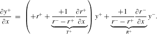 $$\begin{eqnarray}\displaystyle \frac{\unicode[STIX]{x2202}y^{+}}{\unicode[STIX]{x2202}x} & = & \displaystyle \left(+r^{+}+\underbrace{\frac{+1}{r^{-}-r^{+}}\frac{\unicode[STIX]{x2202}r^{+}}{\unicode[STIX]{x2202}x}}_{T^{+}}\right)y^{+}+\underbrace{\frac{+1}{r^{-}-r^{+}}\frac{\unicode[STIX]{x2202}r^{-}}{\unicode[STIX]{x2202}x}}_{R^{+}}y^{-}.\end{eqnarray}$$
 $y^{+}$
and
$y^{+}$
and
 $y^{-}$
experience the opposite effects due to a change in coefficients as mass and energy are conserved.
$y^{-}$
experience the opposite effects due to a change in coefficients as mass and energy are conserved.Symbols


 Open access