


1. Introduction
Many genetic traits relevant to medicine, plant and animal breeding, as well as to evolution are thought to exhibit a complex genetic architecture. Large-scale genetic marker data have become available in recent years making genetic association and mapping studies on genome level possible (McCarthy & Hirschhorn, Reference McCarthy and Hirschhorn2008). These studies aim at identifying multiple genes underlying either a quantitative trait (e.g. human height, plant yield and milk production) or a qualitative trait such as disease status. Major questions of interest are the number of such trait loci, their genomic positions and the magnitude of locus-specific effects on the trait. Classical quantitative genetic theory assumes a great number of genes each with a small effect on a polygenic trait (Fisher, Reference Fisher1918). However, empirical studies indicate that this assumption may be unrealistic as mostly only a few loci, and these with moderate-to-large effects, can be established. The true underlying distribution of effect sizes has been hypothesized to be bell shaped, exponential or leptokurtic (see e.g. Otto & Jones, Reference Otto and Jones2000; Hayes & Goddard, Reference Hayes and Goddard2001; Xu, Reference Xu2003a). Regardless of these assumptions being true for a specific trait or not, limited sample sizes of real datasets prohibit the detection of individual loci with small effects. As a consequence, mixed inheritance models seem plausible in empirical studies. On the one hand, they allow for an oligogenic component as the systemic part to describe effects of detectable trait loci. On the other hand, they merge effects of undetectable loci into a polygenic component. Multiple linear regression provides a suitable statistical framework for analysing the potential associations between complex traits and genotypes.
Multilocus analysis is usually performed using linear regression models where a small subset of loci is selected out of a large number of markers as regressors to the model. This is a model selection problem where a large number of potential regressors and possibly linkage disequilibrium, i.e. correlations among them, complicate the task (see e.g. Broman & Speed, Reference Broman and Speed2002; Sillanpää & Corander, Reference Sillanpää and Corander2002; O'Hara & Sillanpää, Reference O'Hara and Sillanpää2009). For variable selection in genetic association and mapping studies, numerous Bayesian approaches have been proposed. They exhibit several advantages over non-Bayesian methods: multiple testing is not an issue, Bayes factors (BFs) can be used to detect signals of association, and model-averaging across the high-dimensional posterior distribution incorporates the uncertainty of the variable selection procedure into the evaluation of model alternatives.
Bayesian variable selection methods may first fit an over-parameterized model, in which the number of regressors is much larger than the number of individuals. All regressors are simultaneously taken as potential explanatory variables, but shrinkage by means of informative priors is used to force most regressors to have zero or close-to-zero contribution in the model. In the following, our focus will be on different alternatives for shrinkage priors in the context of genetic association and mapping studies. Specifically, we will compare three different shrinkage approaches.
The first one utilizes indicator variables and adaptive Student's t-distributions (IAt) in the specification of priors assigned to gene effects and is a re-formulation of the well-known Bayes B method introduced by Meuwissen et al. (Reference Meuwissen, Hayes and Goddard2001). The second approach is stochastic search variable selection (SSVS) as formulated by George & McCulloch (Reference George and McCulloch1993). In the third approach, we introduce a mixture of uniform priors (MU) as an alternative type of prior specification novel to Bayesian variable selection. We argue that our approach, in contrast to the other two approaches, facilitates the biological interpretation of prior assumptions.
Subsequently, we first describe the multiple regression model in the context of genetic association and mapping studies. Next, we provide details of the prior specification in the three different approaches and compare some of their methodological properties. Then, we spotlight the utility of the Bayes factor in variable selection. We apply Markov Chain Monte Carlo (MCMC) methods as implemented in the publicly available software package OpenBUGS (Thomas et al., Reference Thomas, O'Hara, Ligges and Sturtz2006) to two well-known datasets. Our results consist of a comparison of posterior results yielded by the three different models and an assessment of their MCMC sampling performance under OpenBUGS. Additionally, we evaluate the sensitivity of our approach to the choice of hyperparameters in the prior specification in one of the data examples.
2. Bayesian variable selection
(i) Data model
Consider an association analysis with a population-based sample of distantly related individuals whose phenotypes and genotypes (over marker loci) have been measured. The quantitative phenotype measurements Y i (i=1, …, N) from N individuals are assumed to follow a multivariate normal distribution with mean vector  and variance–covariance matrix σ2 I, where I is the N×N identity matrix. Suppose there are M biallelic markers as potential additively acting trait loci. Genotype observations, say AA, Aa and aa, are coded as 0, 1/2 and 1, respectively, in the N×M model matrix X. Thus, the regression equation takes the form μ=α+Xβ, where the vector
  consists of N entries with the common intercept α and the vector β=(β1, …, βM)T holds the marker effects.
In practice, some genotypes in X may be missing. In a Bayesian set-up, unobserved data points may be treated as additional parameters to be estimated. These nuisance parameters are assigned prior distributions leading to imputation of the missing values according to their emerging posterior distributions. Assuming Hardy–Weinberg equilibrium in the population (see e.g. Hartl & Clark, Reference Hartl and Clark2007, pp. 48–54) and a fixed frequency p for allele A, a natural choice for the treatment of a missing genotype is to assign a multinomial prior distribution with probabilities p 2, 2p(1−p) and (1−p)2 for the genotypes AA, Aa and aa, respectively.
This set-up can be extended to analyse binary traits such as disease status via logistic regression (see e.g. Hosmer & Lemeshow, Reference Hosmer and Lemeshow1989): the phenotype of individual i is modelled as a Bernoulli variable, say Z i with occurrence probability q i=P(Z i=1). Identically to the model above, we describe the vector of logit-transformed occurrence probabilities by regression on the genotype observations, i.e. Q*=α+Xβ, where Q*=(logit(q 1), …, logit(q N))T.
(ii) Sparse variable selection: alternative priors for effect sizes
In a typical genetic association or mapping study, the number of scored markers M is considerably larger than the number of individuals N. Therefore, the previously described data model typically leads to an over-parameterized regression and needs some regularization. Otherwise, the parameters to be estimated remain unidentifiable. If all markers are simultaneously allowed to contribute essentially to the variation observed in the phenotype, the variation of effect size estimates becomes too large for any meaningful inference. Therefore, a model selection problem arises, and it becomes inevitable to choose a smaller subset of markers contributing essentially to the phenotypic variation. In a Bayesian set-up, model selection can be achieved by assigning restrictive, and thus informative, priors to the effect sizes.
In suitable priors, a large fraction of the probability mass is put either directly onto zero or onto a small interval around it, rarely allowing large effects. Simultaneously, they force the majority of markers to explain only an inconsequential part of the phenotypic variation, as measured in the posterior. The graphical form of such priors resembles the shape of a spike (peak at or around zero) and a slab (flat away from zero) (Miller, Reference Miller2002). These priors have also been referred to as spike and smear (see e.g. Ioannidis, Reference Ioannidis2008). In the following, we only consider priors that are symmetric around 0, because there is usually no prior biological knowledge, whether a certain genotype has a positive or negative effect on the phenotype. However, the prior distribution may be truncated to positive or negative values if appropriate.
Typically, a main question of inference in association analysis is the quantification of evidence of whether a marker is to be included into the subset of trait loci. Here, introducing auxiliary indicator variables as a part of the effect size priors supplies a useful means for quantification. The indicator variable obtains value 0 when the effect size is 0 or close to it (spike), and 1 if a non-negligible effect in the slab is detected. The marker occupancy probability in the posterior distribution or BFs provide numerical quantification (see section 4).
Making use of M independent indicators, one for each locus, results in a binomial prior distribution for the number of loci essentially associated with the phenotype with expectation M(1−p 0), when the prior probability of marker exclusion is set to p 0. The sparse selection problem necessitates careful choice of this prior probability: if single-site MCMC sampling is used to approximate the posterior distribution, one would prefer a small value to speed up mixing of the Markov chain, as non-negligible effect sizes would be sampled more often and the whole parameter space could be explored faster. However, as the prior distribution for the number of included markers is binomial, a small value of p 0 would result in a potentially unrealistic high number of associated markers, because the data would hardly have any chance to overcome this strong prior belief. This would increase the risk of overfitting the data and possibly distort the signals and effect sizes from real associations. One should ideally choose p 0 such that–in the specific dataset – a realistic degree of sparseness is obtained and that the MCMC chain still mixes sufficiently ensuring close approximation of the true posterior distribution.
Different strategies exist for utilizing indicator variables in statistical modelling, MCMC sampling and during the inference process:
(a) Indicator variables and adaptive Student's t-distributions (IAt)
When the prior of the effect size is discontinuous at zero (has a ‘lump’), the indicator may be treated as a random Bernoulli variable, say S m, which controls the inclusion/exclusion of marker m. The effect size in the data model can be expressed as the product βm=S mθm (Kuo & Mallick, Reference Kuo and Mallick1998), where θm is a continuous auxiliary variable for a non-zero marker effect. Independently from the prior of S m, the prior of θm is some symmetric distribution on the entire real line or on an interval around zero. Thus, the support of the spike consists only of the point 0 and marker m does not contribute to the likelihood, whenever its indicator S m is 0. The shrinkage of the effect size is adaptive, because the prior specifications of S m as well as θm allow for local, i.e. marker-specific, shrinkage. In MCMC sampling algorithms, the updating schemes for S m and θm should be chosen carefully: if updated in separate steps, θm is sampled from its prior distribution when S m=0. Therefore, a fairly informative prior should be chosen for θm to avoid sampling too often values that lie in areas with low posterior support of βm, which would result in slow mixing of the MCMC chain with regard to S m.
In IAt, each θm is independently assigned a Gaussian prior with mean 0 and its own variance parameter τm2, for which an inverse-gamma distribution with certain constants for the two hyperparameters is assumed. In fact, the marginal prior of the effect size βm=S mθm, (i.e. after integrating over τm2) is mathematically equivalent to the formulation in Bayes B as presented by Meuwissen et al. (Reference Meuwissen, Hayes and Goddard2001), because the prior distribution of βm has a point mass of p 0 (prior probability of marker exclusion) for βm=0 and the marginal prior distribution of θm is a zero-centred and scaled Student's t-distribution (see e.g. Andrews & Mallows, Reference Andrews and Mallows1974). As our formulation of the hierarchical parametrization differs from Bayes B, results concerning the computational efficiency of an MCMC implementation of IAt may not be directly transferable to Bayes B and, to avoid confusion, we refrain from using the same name for the two parameterizations. Given the convergence of MCMC simulation runs, IAt and Bayes B should yield nearly identical posterior estimates, as they both approximate the same posterior distribution.
As in IAt, Sillanpää & Bhattacharjee (Reference Sillanpää and Bhattacharjee2005) used the product βm=S mθm to express the effect size of a genetic marker and chose the same hierarchical parameterization for the scaled Student's t-distribution of θm. Unlike in IAt, however, they induced a dependence structure by assigning a joint Markovian prior to the the set of indicators S m to model linkage disequilibrium among the markers. Also Sillanpää & Bhattacharjee (Reference Sillanpää and Bhattacharjee2006) specified the prior of βm similar to IAt. Here, another indicator variable was added to the product S mθm to assign sample individuals stochastically to two groups. Further, marker indicators S m were group-dependent thus allowing for different sets of associated markers in the two groups.
In Bayes A proposed by Meuwissen et al. (Reference Meuwissen, Hayes and Goddard2001), there is no indicator S m (i.e. βm=θm) and therefore the marginal prior of βm is directly the scaled Student's t-distribution. In a simulation study, Gianola et al. (Reference Gianola, de los Campos, Hill, Manfredi and Fernando2009) demonstrated that Bayes A can be sensitive to the specification of the hyperparameters when predicting genomic breeding values and estimating marker-effects. They argued further that their findings can be directly transferred to Bayes B, because Bayes B is equivalent to Bayes A when no probability mass is assigned to 0 (i.e. p 0=0). In contrast, Verbyla et al. (Reference Verbyla, Bowman, Hayes and Goddard2010) found neither Bayes A nor Bayes B to be sensitive to prior specifications in estimating genomic breeding values in a simulated dataset.
In a comparison of four different shrinkage approaches, Yi & Xu (Reference Yi and Xu2008) used a modified version of Bayes A, where the hyperparameters in the inverse-gamma distribution were treated as random variables. Similarly, Xu (Reference Xu2003a) used a model without marker indicators, but set both the hyperparameters in the inverse-gamma distribution to zero. This leads to an improper prior, namely p(τm2)∝τm−2. Pikkuhookana & Sillanpää (Reference Pikkuhookana and Sillanpää2009) took the approach of Xu (Reference Xu2003a), but included marker indicators in the model and finitely approximated the improper prior.
In this paper, we prefer to use fairly informative values for the hyperparameters (i) to avoid potential problems induced by improper priors, (ii) to ensure the single-site updater to stay in a reasonable range for the values of θm and consecutively also of βm and (iii) to guarantee comparability with results obtained from the other two approaches as described in the following.
(b) SSVS
In contrast to the discontinuity at the origin in the previous choice of prior, the probability mass of the spike is concentrated on a small interval around zero in SSVS as proposed by George & McCulloch (Reference George and McCulloch1993). Both the spike and the slab have zero-centred normal distributions, the spike having a small variance, say t 2, and the slab a large variance, say c 2t 2 with c≫1. Bernoulli distributions for the indicator variables S m control the a priori mixture proportions of the spike and the slab: βm~p 0N(0, t 2)+(1−p 0)N(0, c 2t 2), where p 0=P(S m=0). Here, the support of the spike and that of the slab are not distinct, but they are in fact the same: the entire real line. Therefore, the interpretation of S m as an indicator for marker inclusion/exclusion in the model does–strictly speaking–not hold: βm obtains non-zero values almost surely, and thus marker m always contributes to the likelihood, irrespective of the value of S m. Unlike in IAt, the likelihood in SSVS contains only βm but not the indicator S m directly. Merely, the indicator controls whether the effect size comes from the spike or from the slab. In practice, however, the spike will be sufficiently narrow, if the hyperparameters are appropriately chosen. When S m=0, it will allow only such small values of βm that such marker effects can be considered ineffective or negligible in their contribution to the likelihood.
Typically, pilot MCMC simulations are run to tune the hyperparameters thus ensuring good mixing properties of the final MCMC chain. Alternatively, Meuwissen & Goddard (Reference Meuwissen and Goddard2004) gave t 2 its own prior and treated it as a random parameter to be estimated with the other parameter c 2 being fixed. In the prediction of breeding values for genomic selection purposes, Verbyla et al. (Reference Verbyla, Bowman, Hayes and Goddard2010) found this model (Bayes C) along with Bayes A as well as Bayes B (see previous section) also to be insensitive to prior specifications. In the context of variable selection, however, O'Hara & Sillanpää (Reference O'Hara and Sillanpää2009) noticed that this approach appears sensitive to the choice of the mixing ratio c 2 of the two variances and may lead to poor separation capability in distinguishing between true and false associations. In this study, we chose to fix the two hyperparameters, c 2 and t 2, to ensure the comparability of the prior specification with the other two approaches.
During MCMC, the indicator variables are usually treated as auxiliary parameters and updated in each iteration of the sampling scheme. Therefore, posterior occupancy probabilities are readily available for inference concerning S m. Although convenient for inference and mostly used, the explicit sampling of S m would actually not be necessary, because the prior of βm as well as its fully conditional posterior distribution have continuous density functions that could be directly exploited in a Metropolis–Hastings updating step or during Gibbs sampling, respectively.
(c) Mixture of uniform priors
In this paper, we introduce a new class of spike-and-slab–shaped priors for effect sizes. These priors aim at fulfilling the following two properties: (i) hyperparameters controlling the extent of the spike and the slab have a direct biological interpretation, which simplifies the specification of realistic priors based on expert knowledge; (ii) to ensure good simulation performance, only one parameter per marker should be updated during MCMC, i.e. separate sampling of indicator variables and effect size values is avoided.
In our formulation, the prior density function  for a marker effect βm arises from a mixture of three distinct uniform distributions on all loci m=1, …, M:
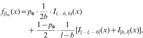
where I A(x) is the indicator function of a set A, i.e. it obtains value 1 if x∊A and 0 otherwise, and 0<b<l are constants to be specified. The mixing proportion p 0∊(0,1) controls how much probability mass is assigned to the interval around zero with borders (−b, b). The effect size is limited to the interval (−l, l). In this formulation, the supports of the spike and the slab are distinct, (−b, b) for the spike and (−l, −b]∪[b, l) for the slab. Figure 1 illustrates the prior density of this kind. In order to obtain a posterior value for the occupancy probability of marker m, we construct an indicator variable as a direct function of the effect size. We define the indicator as S m=1−I (−b, b) (βm), whose posterior distribution is exploitable during posterior inference. Note, however, that it is not necessary to sample S m during MCMC simulation.
Prior density of an effect size βm with probability of marker exclusion p 0, border value b and upper limit l.
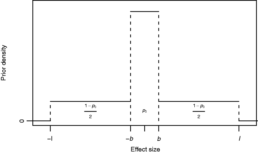
The biological interpretation of the three hyperparameters (p 0, b and l) to be specified is straightforward to conceptualize: the prior probability that the absolute value of the effect size is smaller than b is p 0, and this prior does not allow effect sizes larger than l. Although marker m contributes to the likelihood for any value of βm, we may consider effect sizes smaller than b as biologically negligible in this context and may consequently interpret that the marker is not essentially associated with the phenotype, i.e. is not a trait locus. This is undoubtedly a simplistic interpretation, but on the other hand in agreement with the empirical support (see Mackay, Reference Mackay2001, and references herein) suggesting that quantitative variation cannot be explained by a very large number of trait loci with very small effects, but that it merely arises from a distribution of effect sizes resembling some exponential distribution as proposed by Robertson (Reference Robertson and Brink1967). Further, the number of individuals in the sample as well as the allelic frequencies at single loci restrict the ability to detect small gene effects and will therefore affect the choice of b. Similarly, coarseness of measurement complicates detection of small effect sizes, since such noise in the data weakens the possibility of detecting signals from small effects.
The upper limit l restricts the range of the values that the effect size βm can obtain. Its specification should allow effect sizes expected to be seen in the data under the experimental design in question. Such an upper limit may be hard to determine a priori, but expert knowledge in form of the empirical evidence that effect sizes of single trait loci are typically not larger than a couple of phenotypic standard deviations can serve as guideline: e.g. large locus effects on bristle number in Drosophila are mostly between 0·5-and 2 phenotypic standard deviations (Mackay, Reference Mackay1996), and Hayes & Goddard (Reference Hayes and Goddard2001) reported a maximal additive locus effect size of 1·2 phenotypic standard deviations in a meta-analysis of quantitative traits in livestock.
As will be shown below in the sensitivity analysis of our approach, the specification of the effect size limit l can seriously affect posterior estimates. This is alarming, because altering l only affects the width of the slab (i.e. the tails of the distribution). Of course, posterior results should ideally not be influenced by the width of the tails. Clearly, this problem is common to all the three spike-and-slab approaches considered in this study, because they share the assumption of relatively flat tails in the respective prior distributions and the widths of the tails are specified via hyperparameters. In principle, this problem could be targeted at by treating the hyperparameters influencing the tails as random variables and trying to estimate them from the data. Successful identification of these parameters can only be expected, if effect size parameters get estimated with high precision and enough markers are estimated with large effects providing the necessary information on the tails of the distribution. While the precision of effect size estimates can be improved by increasing the sample size, the number of markers with large effects is limited by the genetic architecture of the trait: as mentioned in the introduction, empirical studies indicate that even with dense marker sets only a few loci with large effects can be identified for many traits resulting in poor identifiability of the tails.
3. MCMC and sampling performance
We implemented the three models presented above in the BUGS script language, and ran MCMC simulations in OpenBUGS version 3.0.3 via the R-package BRugs version 0.4–3 (Thomas et al., Reference Thomas, O'Hara, Ligges and Sturtz2006). The BUGS script is provided in the Supplementary material.
In order to assess sampling performance of the competing models with respect to marker indicators, we first calculated the number of switches between 0s and 1s for sequences of marker indicator MCMC samples. Then, we divided this number by computation time to attain comparability across the competing sampling algorithms. As the number of switches is strongly influenced by the marker's occupancy probability, i.e. the proportion of 1s in the sequence, results for different markers within the same model cannot be compared. However, if occupancy probabilities are close to each other in competing models, marker-specific number of switches can be used to compare model performance.
Additionally, we assessed computational performance of the three models by calculating effective sample sizes (ESS). Specifically, we used the initial positive sequence estimator as proposed by Geyer (Reference Geyer1992) to estimate the cumulative lagged autocovariances in the MCMC sampling sequences of each effect size parameter βm. Thus, we obtained the MCMC errors of the posterior means needed to calculate ESS. Again, the division of ESS by computation time makes comparison across models possible (see Waagepetersen et al., Reference Waagepetersen, Ibánẽz-Escriche and Sorensen2008). The interpretation of ESS for a Monte Carlo estimate (here the mean of βm calculated across MCMC iterations) is, how many independent samples one would need to generate to obtain the same precision of this estimate as obtained from Markov Chain sampling, where consecutive samples are autocorrelated. Thus, ESS divided by computation time can be used to compare the sampling performance of posterior mean estimation, as long as the marginal posterior distributions of the effect sizes yielded by the different MCMC samplers are reasonably close to each other.
4. Posterior inference on marker occupancy and BFs
In genetic association and mapping studies, the main focus is to quantify the importance of a marker with respect to its influence on the trait in question. The variable selection methods above provide the posterior distribution of the dichotomous marker indicators to address this question.
This posterior can be explored in terms of marker occupancy probabilities during MCMC, i.e. we count in how many iterations a certain marker obtains value 1 and calculate the corresponding occupancy probability by dividing this count by the total number of MCMC iterations. When interpreting this posterior probability, we have to keep in mind that the prior specification does not necessarily correspond to expert prior knowledge as conventionally intended in the Bayesian paradigm. Merely, as mentioned in section 2 (ii), we have to carefully control p 0 (prior probability of marker exclusion) to obtain a realistic degree of sparseness in the multilocus model and to guarantee sufficient mixing of the MCMC chain. Therefore, we are not completely free in assigning a prior probability that would correspond to expert prior knowledge.
Next to posterior probabilities, BFs provide an alternative measure of evidence. For dichotomous variables, such as a marker indicator S m, the BF is simply calculated as the ratio of posterior odds to prior odds (Kass & Raftery, Reference Kass and Raftery1995):
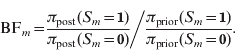
Following Jeffreys (Reference Jeffreys1961), the BF values can be classified into categories characterizing the strength of evidence they suggest against the hypothesis H 0:S m=0 (or against H 1:S m=1):
• evidence ‘not worth more than a bare mention’: a BF between 1 and 3 (0·3 and 1),
• ‘substantial’ evidence: a BF between 3 and 10 (0·1 and 0·3),
• ‘strong’ evidence: a BF between 10 and 100 (0·01 and 0·1),
• ‘decisive’ evidence: a BF above 100 (below 0·01).
We use these evidence limits in the graphical presentation of the results (left panel of Fig. 3 and Fig. 6 a).
For any two hypotheses, the BF is defined as the ratio of the marginal likelihoods of the two hypotheses, say Pr(data|H 1)/Pr(data|H 0). As pointed out by Satagopan et al. (Reference Satagopan, Yandell, Newton and Osborn1996), stable estimation of these marginal likelihoods can be challenging depending on the complexity of the models the hypotheses represent. Estimation of the BF for marker occupancy, as seen above, is straightforward and does not require demanding computations, because the two competing hypotheses concern only the status of the dichotomous marker indicator.
As can be seen from the general definition of the BF with regard to two arbitrary hypotheses, its estimation corresponds to calculation of two marginal likelihoods, which involves integrating over parts of the parameter space, i.e. different models with varying parameter values are weighted according to their respective probabilities under the hypothesis in question. Hence, the ratio of two marginal likelihoods, i.e. the BF, is a model-averaged measure for the evidence against H 0, somewhat similar to the conventional likelihood ratio test statistic. However, the conventional likelihood ratio test statistic is based on only two models, namely those two that maximize the likelihood of the data under the two hypotheses, thus ignoring uncertainty induced by the existence of model alternatives. Additionally, the likelihood ratio only provides a means to compare nested models, whereas such a restriction does not apply to the use of BFs, as H 0 and H 1 can be freely chosen.
5. Examples
(i) Barley data
(a) Description of the data and specification of the prior
The data originate from the North American Barley Genome Mapping Project (Tinker et al., Reference Tinker, Mather, Rossnagel, Kasha, Kleinhofs, Hayes, Falk, Ferguson, Shugar, Legge, Irvine, Choo, Briggs, Ullrich, Franckowiak, Blake, Graf, Dofing, Saghai Maroof, Scoles, Hoffman, Dahleen, Kilian, Chen, Biyashev, Kudrna and Steffenson1996). The plant material consisted of 150 two-row barley (Hordeum vulgare L.) double-haploid lines, for which seven agronomic traits were monitored. Here, we only analysed one of the traits: days to heading. We excluded five double-haploid lines due to missing trait observations (one line) or completely missing genotypes (four lines). As the trait was monitored in 25 different environments, we averaged the observations across the environments for each double-haploid line. Here, we report results based on the standardized scores of these 145 means, which were used as quantitative phenotype measurements. In case of double-haploid lines, the genotype data in X comprise dichotomous observations, say genotypes AA and aa, for each marker. Here, 127 markers on seven linkage groups were scored. Nine hundred and thirty genotype observations (5·1%) were missing.
The prior distributions assigned to the gene effects, βm, are illustrated in the left plot of Fig. 2. As the density function of the prior of βm is not defined at 0 for IAt, we present the cumulative distribution functions (CDF) to allow comparison. We deliberately choose the values of the hyperparameters in IAt, SSVS and MU so that the distributions would resemble each other. As can be seen in the figure, the distributions are visually distinguishable only in the tails of the distributions. In the following we give the numerical values for the hyperparameters used in the prior specifications.
Comparison of prior distributions in IAt (blue), SSVS (red) and MU (black). The curves indicate the CDF of the prior distributions assigned to gene effects βm in the analysis of the Barley data (left) and the CF data (right).

We assumed the following priors for the parameters shared by all three models: for the intercept parameter α a normal distribution with mean 0 and variance 106, for the residual variance σ2 an inverse-gamma distribution with shape parameter 0·01 and scale parameter 100, and for missing genotype observations in the model matrix X Bernoulli distributions with probability 0·5. In all three models, the prior exclusion probability was set to p 0=0·89 for each marker. Therefore, in both IAt and SSVS, the model parameters S m were given Bernoulli priors with probability 1−p 0=0·11. This choice for p 0 was arbitrary; we address the question of the influence of this choice below in the sensitivity analysis for MU.
In IAt, the marker-specific effect size variances τm2 were given inverse-gamma prior distributions with shape 1 and rate 1. In SSVS, we set the variances of the spike and the slab to t 2=1·1×10−5 and c 2t 2=0·15, respectively. In MU, we used the border value b=0·01. Here, this corresponds to a minimal effect size of 1% of the phenotypic standard deviation, because we analysed a standardized score. Likewise, we allowed for a maximal effect size of one phenotypic standard deviation by setting the limit value to l=1.
(b) Comparison of posterior estimation
The three models yielded slightly different estimates for the summary statistic  , which counts the indicators with value 1 across loci and aims at estimating the number of trait loci in the marker data. Keeping in mind that the individuals are from a double-haploid population, the conclusions that can be drawn from the estimates of N Q with respect to the genetic architecture of the trait are very limited. The posterior mean of this combined parameter was smallest for IAt with 17·5. For MU and SSVS, the posterior means were 19·0 and 22·9, respectively. Thus, IAt estimated more parsimonious models than the other two. However, the mean number of trait loci was estimated higher in all three models when compared with the prior assumption assigned to this parameter, M(1−p 0)=14·0.
The observation that IAt produced the most simple models was corroborated by the residual variance: posterior estimation showed the highest residual variance for IAt with a maximum a posteriori (MAP) estimate of 0·14, and 0·08–0·25 as the 95% credible interval with the 2·5% quantile as lower, and the 97·5% quantile as upper bound (95% CI). For MU and SSVS, the MAPs and 95% CIs were 0·11 (0·07–0·22) and 0·12 (0·06–0·21), respectively. As we were analysing a standardized trait, we obtained MAP estimates for heritability by calculating h 2=1−σ2, which yielded 0·86 for IAt, 0·89 for MU, and 0·88 for SSVS.
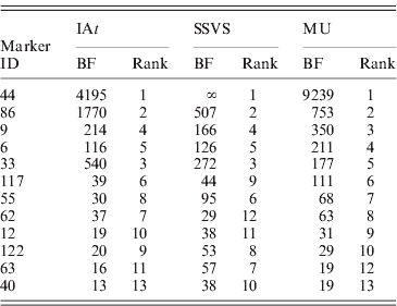
Table 1 reports BFs for marker occupancy of 12 loci with strongest evidence according to all three models. Notably, all three models identified the same five markers to have the highest BFs, all of them being above 100. The left panel of Fig. 3 shows the BFs for the remaining 115 markers illustrating their comparability among the three models: the majority of markers fell within the same categories of strength of evidence (see section 4) for all the three models.
Results for the Barley data. Left panel (a–c): Bayes factors (BFs) for marker occupancy on logarithmic scale. The 12 BFs reported in Table 1 are not shown. Dashed lines indicate the borders of the BF categories of strength of evidence (see section 4). Right panel (d–f): Bland–Altman plots for effect sizes of 127 markers.

Comparison of Bayes factors (BFs) for marker occupancy and ranks in the three competing models (Barley data). Results of 12 markers that are among the 10 markers with highest BFs in at least one model.
The Bland–Altman plots (Altman & Bland, Reference Altman and Bland1983) for the posterior means of the effect sizes in the right panel of Fig. 3 show that estimates of the effect sizes did not systematically differ in the three models.
(c) Performance of MCMC simulation
Computation of 40 000 iterations took 235 min for MU, 666 min for IAt and 234 min for SSVS. The left panel of Fig. 4 shows the number of switches between 0s and 1s per minute of computation time for each marker indicator in the three competing models. MU showed best performance with respect to this indicator of mixing property: for MU, the number of switches per minute was on average 1·4 (median: 1·4) times higher than for IAt, and 2·1 (median: 1·7) times higher than for SSVS. When compared with SSVS, IAt performed better with on average 1·4 (median: 1·2) times more number of switches per minute.
Results for the Barley data. Left panel (a–c): number of switches per minute during MCMC simulation for 127 marker indicators. Right panel (d–f): Bland–Altman plots for ESS/min for 127 posterior means of effect sizes.

The right panel of Fig. 4 shows Bland–Altman plots of effective sample sizes per minute (ESS/min) of computation time for each effect size parameter in the three competing models. Also here, MU showed best performance: it yielded on average 1·6 ESS/min more than IAt (median: 0·8), and 2·0 (median: 0·7) more than SSVS. SSVS had better performance than IAt according to this criterion, with the average number of ESS/min being 0·5 more in SSVS than in IAt (median: 0·0). However, the picture from this performance measure was less pronounced than for the indicators: we observed 107 (of 127) effect sizes with higher ESS/min in MU than in IAt; 109 times the number was higher in MU than in SSVS, and 74 times higher in SSVS than in IAt.
(d) Sensitivity analysis
In order to assess the sensitivity of our proposed model MU to the choice of the three hyperparameters p 0, b and l, we estimated the posterior distribution via MCMC simulation under eight different prior specifications of these hyperparameters. We assigned two substantially different values to each parameter (p 0=0·99 or 0·79, b=0·01 or 0·1, l=1 or 10) and formed all possible parameter triplets with these values. All other prior parameters were specified as before. Table 2 shows the prior specifications of the eight MCMC chains and posterior estimates for the number of occupied markers N Q and the residual variance σ2 and Fig. 5 occupancy probabilities of all markers. For reference, the positions of markers reported in Table 1 as well as threshold lines corresponding to a BF of 10 are also represented in Fig. 5.
Marker occupancy probabilities for the eight MCMC chains A–H used to assess the sensitivity of model MU on the analysis of the Barley data. The vertical lines indicate the markers with the highest (BFs) for marker occupancy as reported in Table 1. The horizontal lines indicate the probability levels corresponding to BFs of 10 under the respective values of p 0 (0·99 in chains A–D and 0·79 in chains E–H).

Prior specifications and posterior estimates for the eight MCMC chains A–H used to evaluate the sensitivity of model MU on the analysis of the Barley data. The summary statistic  is the number of occupied markers and has prior mean E(N Q)=M(1−p 0). The lower and upper limits of the reported credible intervals (95% CI) are the 2·5% and 97·5% quantiles, respectively. The point estimate used for the residual variance σ2 is the MAP estimate.
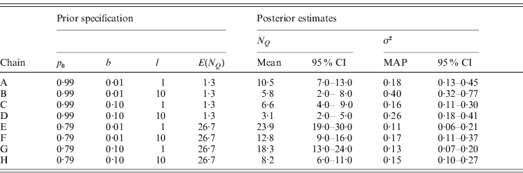
As expected, chains A–D with higher p 0 yielded sparser models as reflected in the smaller posterior estimates of N Q when compared pairwise with chains E–H. Correspondingly, more phenotypic variation remained unexplained in chains A–D as indicated by the larger posterior estimates for σ2. Notably, the prior mean of N Q with value 1·3 in chains A–D is smaller than the corresponding posterior means estimated with values ranging between 3·1 and 10·5, whereas the prior mean of N Q is higher than the posterior estimates (8·2–23·9) in chains E–H. The marker occupancy probabilities in Fig. 5 also show that the chains with p 0=0·99 (A–D) yielded sparser models, as these estimates are close to 0 for most markers. In contrast, three of the chains with p 0=0·79 (E–G) produced noisy pictures with considerably more markers obtaining posterior estimates away from 0. Although the noise in chain H is less pronounced than in chains E–G it is still somewhat more than in chain D.
The pairwise comparisons of chains A, B, E and F with smaller border value b against chains C, D, G and H also yielded results as expected: choosing a small value for b facilitates the indicator variables S m to obtain value 1 and accordingly the posterior estimates of N Q were estimated larger for smaller b indicating less sparse models. Correspondingly, occupancy probabilities are found notably above 0 at more markers in chains A, B, E and F in these pairwise comparisons. In three out of the four comparisons, σ2 was estimated higher reflecting more variation unexplained for smaller b. The exception was the comparison of chains E and G, where the point estimates and the 95% credibility intervals of σ2 were very similar.
Changing the maximal effect size limit l from 1 to 10 notably increased the posterior estimates for σ2 and reduced the posterior estimates of the number of occupied markers N Q as seen in the pairwise comparisons of chains A, C, E and G with chains B, D, F and H, respectively. As seen from Fig. 5, also the estimation of occupancy probabilities was seriously affected. As mentioned earlier in the description of the MU approach, this result is alarming, because altering the maximal effect size limit l only affects the width of the slab (the tails of the prior distribution of βm) and should not influence posterior estimates. However, similar sensitivity to the specification of the tails is expected to be seen in any spike-and-slab approach where the tails are determined via hyperparameters. We should also note here that setting l=10 was a deliberately extreme choice for this parameter in the light of locus effects being probably not larger than 2 phenotypic standard deviations for many quantitative traits (cf. Mackay, Reference Mackay1996; Hayes & Goddard, Reference Hayes and Goddard2001). Evidently, restricting l to a more realistic value would have resulted in the sensitivity appearing less strong.
(ii) Cystic fibrosis (CF) data
(a) Description of the data and specification of the prior
We also analysed a second well-known dataset, in which the phenotype is a binary disease status, using logistic regression as described in section 2 (i). We used the data on 92 haplotypes of individuals affected with CF and 94 control haplotypes (N=186) as reported by Kerem et al. (Reference Kerem, Rommens, Buchanan, Markiewicz, Cox, Chakravarti, Buchwald and Tsui1989). The data contain observations of M=23 biallelic restriction fragment length polymorphism (RFLP) markers ranging over a 1·8 Mb candidate region on human chromosome 7 (region q31). The marker data consist of distinct haplotypes, rather than diploid genotype data, and haplotype pairs belonging to the same individuals cannot be matched. Therefore, we had to perform the analysis based on a double-sized sample, in which each individual is represented twice, although such analysis has been criticized (cf. Sasieni, Reference Sasieni1997). One hundred and sixty-nine allelic observations (4·0%) were missing.
As for the Barley data analysis, we give a graphical illustration for the prior distributions assigned to the gene effects, βm (right plot of Fig. 2). As above, the hyperparameters were deliberately chosen so that the distributions would resemble each other for IAt, SSVS and MU.
In all three models, we chose an arbitrary value for p 0 and set p 0=1−1/M=0·957. The intercept parameter α was assigned a normal distribution with mean 0 and variance 106. All missing alleles were imputed by assigning Bernoulli priors with probability 0·5. In IAt, each marker-specific variance for the effect size τm2 was assigned an inverse-gamma prior distribution with shape parameter 1 and rate parameter 1. In SSVS, we used a value of t 2=2·28×10−4 for the prior variance of the spike, and a value of c 2t 2=3·77 for the prior variance of the slab. The border value in MU was set to b=0·05 and the limit of the effect sizes to l=5.
(b) Comparison of posterior estimation
More parsimonious models were favoured by MU than by the other two models, with the posterior means of the summary statistic  being 2·6 in MU, 2·9 in SSVS and 3·1 in IAt. Here, we should note that N Q aims at estimating the number of trait loci found in the marker data. As the marker data are from a 1·8 Mb candidate region, i.e. only a very small fragment of the human genome, N Q cannot estimate the total number of trait loci found in the entire genome and does therefore not allow any conclusions with respect to the genetic architecture of the trait. Table 3 shows the posterior distribution of N Q under the three models and its prior binomial distribution. The modes of the distributions show that MU supported models with two trait loci in the data, IAt models with three trait loci, whereas SSVS yielded models with two or three trait loci almost equally likely.
Prior and posterior distributions of the summary statistic  (number of occupied markers) for the CF data.
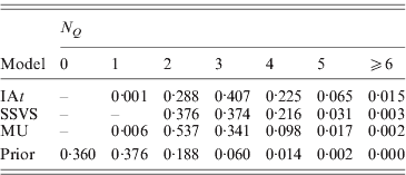
Fig. 6 a shows the marker-specific BFs for marker occupancy in the three models. All models distinctly identified signals of at least ‘strong evidence’ for markers 10 and 17 according to their BFs. For marker 17, the BFs in the three models agreed well with values between 64 and 77. For marker 10, IAt and MU yielded comparable BFs of 70 and 77, whereas the BF in SSVS was remarkably high with 5692. There were also signals of ‘substantial evidence’ with BFs between 4 and 9 for markers 2 and 18 in all three models. Also the estimated effect sizes (Fig. 6 c) suggested strong trait loci at positions 10 and 17 and weaker ones at positions 2 and 18.
Results for the CF data. (a) Bayes factors (BFs) for marker occupancy on logarithmic scale. Dashed lines indicate the borders of the BF categories of strength of evidence (see section 4). (b) MCMC switches per minute for marker indicators. (c) Posterior means of effect sizes on logistic liability scale. (d) MCMC effective samples per minute (ESS/min) for effect sizes.

Previous studies identified the same markers as reported here. The 20-kb region between markers 17 and 18 is known to contain the ΔF 508 mutation, a 3-bp deletion found in 66% of CF chromosomes worldwide (Bertranpetit & Calafell, Reference Bertranpetit, Calafell, Chadwick and Cardew1996). Molitor et al. (Reference Molitor, Marjoram and Thomas2003) as well as Sillanpää & Bhattacharjee (Reference Sillanpää and Bhattacharjee2005) reported associations between CF and markers 10 and 17 making use of marker map information. Molitor et al. (Reference Molitor, Marjoram and Thomas2003) used a single-locus model for marker position and found a bimodal distribution with peaks at locations corresponding to markers 10 and 17. Sillanpää & Bhattacharjee (Reference Sillanpää and Bhattacharjee2005) used the smoothed distances to control for between-marker correlations in a multilocus model. The less pronounced effect at marker 2 has also been observed by Lazzeroni (Reference Lazzeroni1998) using marker-specific estimates of linkage disequilibrium. Sillanpää & Bhattacharjee (Reference Sillanpää and Bhattacharjee2006) derived stochastically two etiological subgroups from the data, and found a strong association at marker 2 within the smaller subgroup consisting of around 20% of the haplotypes.
(c) Performance of MCMC simulation
Computation of 40 000 iterations took 79 min for SSVS, 115 min for IAt and 153 min for MU. IAt clearly outperformed the other two models with respect to the number of switches per minute of computation time for marker indicators (see Fig. 6 b). MU performed better than SSVS with on average 4·8 times more number of switches/minute (median: 2·6), with higher values at 20 of the 23 markers. When comparing the three models by ESS/min for effect sizes (see Fig. 6 d), again IAt showed the best performance with highest ESS/min at 21 loci.
6. Discussion
We have presented a new approach (MU) to specify slab-and-spike priors for Bayesian variable selection in genetic association and mapping studies. We illustrated its application as well as its performance in two genetic datasets. We have also compared its computational efficiency in MCMC estimation with two other approaches (IAt and SSVS) used to identify multiple trait loci. Under the chosen prior specifications, the three models yielded similar results with respect to trait locus detection. We observed fairly high sensitivity of posterior estimation to the prior specifications in MU. The high sensitivity is likely due to the considerable differences in the choice of the hyperparameters we used for the sensitivity analysis. We further argue that the other two approaches and any other spike-and-slab approach requiring hyperparameters are similarly sensitive, because altering hyperparameters affects the forms of the spike and the slab.
The differences in computational efficiency reported here only reflect the performance of sampling schemes as implemented in OpenBUGS, and can–at best–be a guide to choose between the three models when OpenBUGS is used. Further, even for OpenBUGS the differences between efficiency statistics reported here do not unequivocally favour any one of the three models: the most efficient approach in the linear model used for the Barley data appears to be MU, whereas IAt seems superior when applying logistic regression to the CF data. This is arguably attributable to the differences in implementation of the linear and logistic models in OpenBUGS. The computation times required for MCMC simulation in the two data examples suggest that run-times in OpenBUGS remain at reasonable levels for studies with a few hundreds of markers at most.
Our study does not give any indication that the posterior results yielded by MU are in any way inferior or superior when compared with the other two approaches. In contrast, we specified the hyperparameters in the three models in such a way that the priors resembled each other and MCMC estimation yielded similar results. Thus, the only obvious benefit of MU lies in the more straightforward interpretation of the the hyperparameters, until a more efficient MCMC sampler is available. This is currently being worked on.
The main target in variable selection problems is to answer the question, whether we should consider a potential explanatory regressor to influence the outcome or not. This question is addressed by testing some statistical hypothesis. Specifically, testing marker inclusion means deciding in favour of or against a precise null hypothesis. The precise null hypothesis can be formulated in terms of a point null or an interval null (see Berger & Delampady, Reference Berger and Delampady1987; Berger & Sellke, Reference Berger and Sellke1987). The latter corresponds to relaxing our conception of precise in the sense that a marker may exhibit some minuscule effect on the trait, which is, however, to be considered as of no practical interest. Use of BFs as a measure of evidence in genetic association and mapping studies has been motivated, at least, by the following properties: (1) they are similar to the likelihood ratio statistic, i.e. the evidence is compared against a null model (Lee & Thomas, Reference Lee and Thomas2000), (2) they are able to combine evidence from multiple data sources (see Ball, Reference Ball2007; Wakefield, Reference Wakefield2008), (3) they provide interpretation (unlike P-values) independent from sample size (Wakefield, Reference Wakefield2009) and (4) ‘(they) may be used routinely to interpret ‘significant’ associations' (Ioannidis, Reference Ioannidis2008).
A common approach for estimation-based variable selection in Bayesian multilocus models is to fit scaled zero-centred Student's t-distributions to effect size parameters. These distributions are controlled by two parameters: (a) the degrees of freedom determining the peakedness as well as the heaviness of the tails and (b) the scale parameter determining the dispersion in the distribution. Here, the peakedness of the distribution controls the degree of sparseness in the selected markers, whereas the dispersion in the distribution relates to the range of possible effect size values. In IAt, Student's t-distributions are obtained by applying a hierarchical prior consisting of normally distributed effect sizes each with its own variance parameter. IAt, however, extends the common Student's t approach by introducing another means to control for sparseness in the model. The Bernoulli indicator variables control inclusion/exclusion of a marker. Thus, a third parameter contributes to the set-up of priors, namely, the prior probability of the Bernoulli distribution. As IAt is in fact an alternative parametrization of the well-studied Bayes B approach proposed by Meuwissen et al. (Reference Meuwissen, Hayes and Goddard2001), posterior estimates should be identical, but our results concerning the computational properties for the MCMC implementation of IAt are not transferable to Bayes B.
As in IAt, three parameters specify the prior set-up of the effect size parameters in SSVS: here, the Bernoulli probability of the marker indicators determines the mixing proportion of the spike and the slab, whose variances are then controlled by the two remaining parameters. Whereas in IAt and SSVS only the Bernoulli probability of the marker indicator offers a direct biological interpretation, also the other two parameters used in the prior set-up of MU are straightforward to interpret: the border value b directly states when an effect size is to be considered negligible, and the other parameter l restricts the range of effect sizes to a realistic limit.
As seen in our sensitivity analysis, posterior results heavily depend on the assumptions concerning the tails of the prior distribution assigned to effect sizes. As large effects appear to be rare phenomena in complex traits, there is little hope that single studies or even meta-analyses could provide enough information to identify these tails for a specific quantitative trait. Additionally, genetic association and mapping studies generally suffer from the Beavis effect (Lande & Thompson, Reference Lande and Thompson1990; Beavis, Reference Beavis and Paterson1998; Xu, Reference Xu2003b): limited sample size prohibits identification of trait loci with small effects and leads to the ‘winner's curse’ of detected loci, i.e. effect sizes of trait loci are typically overestimated and cannot be replicated in follow-up studies due to underpowered study designs (Lohmueller et al., Reference Lohmueller, Pearce, Pike, Lander and Hirschhorn2003; Xiao & Boehnke, Reference Xiao and Boehnke2009). Therefore, trying to estimate effect sizes and identify the tails of a slab-and-spike distribution simultaneously could yield a biased picture not only for effect sizes but for the tails as well. It therefore appears reasonable to treat a parameter used to specify the width of the tail, such as l in MU, as a hyperparameter to be specified and rely on prior knowledge or even assumptions independent from the data to be analysed.
Whereas the indicator variables (S m) are treated as model parameters in IAt and SSVS and are sampled during MCMC simulation, both the adaptive shrinkage method of Xu (Reference Xu2003a) which makes use of an improper prior, as well as MU avoid sampling of indicator variables. However, there is one important difference between the approach of Xu (Reference Xu2003a) and MU: the former lacks the prior control for the degree of sparseness in the model. On the other hand, this lack of control can also be seen as an advantage: the posterior distribution in the model of Xu (Reference Xu2003a) can summarize the degree of sparseness from the information in the data and relatively vague prior assumptions. However, if the information in the data is too little or the degree of sparseness should reflect our biological assumptions concerning the number of trait loci, the direct control of sparseness provided in MU is an advantage over the shrinkage approach of Xu (Reference Xu2003a) .
Genomewide application of any of the three models presented here to thousands or even a larger number of markers would require MCMC simulation by another means than OpenBUGS. More efficient MCMC implementations and algorithms are topics for future research. With limited computer resources in mind, recent developments in computationally fast approximative Bayesian methods not relying on MCMC simulation present an attractive alternative, especially for large-scale studies. These include the design of fast expectation–maximization (EM) algorithms, as e.g. done by Yi & Banerjee (Reference Yi and Banerjee2009) to find the posterior modes of the effect size parameters and by Xu (Reference Xu2010) to obtain empirical Bayes estimates. In order to estimate genomic breeding values, Hayashi & Iwata (Reference Hayashi and Iwata2010) modified the algorithm by Yi & Banerjee (Reference Yi and Banerjee2009), whereas Meuwissen et al. (Reference Meuwissen, Solberg, Shepherd and Woolliams2009) constructed an iterative conditional expectation algorithm. All these studies reported at most moderate losses in accuracy of point estimates when compared with computationally much more intensive MCMC-based methods.
This work was supported by the Finnish Graduate School of Populations Genetics and by research grants from the Academy of Finland and the University of Helsinki's Research Funds. We would like to thank two anonymous referees for their constructive comments and suggestions, which considerably helped us to improve the manuscript. TK would like to thank Petri Koistinen for useful discussions about ESS estimates.
7. Supplementary material
The online data are available at http://journals.cambridge.org/GRH.



