Study site location and climatology

Our study site was near Summit Camp, Greenland (72.68 N, 38.58 W; 3200 ma.s.l.), 28km west of the GIS summit. The mean annual accumulation at Summit is ∼24.0±0.5cm w.e. a-1 (Reference MeeseMeese and others, 1994), with a mean annual temperature of -328C (Reference Drab, Gaudichet, Jaffrezo and ColinDrab and others, 2002). Reference Alley and AnandakrishnanAlley and Anandakrishnan (1995) investigated melt feature incidence in the deep Greenland Ice Sheet Project 2 (GISP2) ice core from a nearby site and observed a frequency of one melt event per 250 years over the last 3 ka.

Experimental design

We conducted a total of four melt experiments in separate snow pits to investigate the influence of percolating and refreezing meltwater on trace-element chemistry. We arranged the four snow pits in pairs separated by 6km; neighbouring pits were 10 m apart. Thus, each experiment has one neighbour experiment 10m away, and two experiments 6 km away.

For each melt experiment, we filled a pre-cleaned polyethylene carboy with surface snow collected from the top 3 cm of the snowpack. The snow was melted inside the carboy in a heated, interior space, and then cooled until the temperature of the meltwater approached 08C. We constructed a meltwater applicator consisting of a perforated, 1 m long narrow plastic cylindrical sleeve, sealed at one end and open at the other, using low-density polyethylene ‘layflat’ plastic (typically used to protect ice cores during transport). Both the carboy and applicator were triple-rinsed with MilliQ (>18.2Mfi) deionized water before use. We applied ∼15 L of meltwater across an 80 x 80 cm² area of the snow surface for each melt experiment. This amount of melt application conservatively approximates an annual melt percentage of 10%. The meltwater was allowed to penetrate into the snow for 2-4 hours in pits 1-3 before sampling, and for 33 days in pit 4. Although the amount of water applied and its rate of application is not representative of typical melt events at our field site, we aimed to supply sufficient water to allow for water infiltration through at least 1 year of accumulated snow. This also allowed for infiltrating meltwater to interact with impeding stratigraphic features, such as impermeable layers or grain-size transitions that act as capillary barriers, both of which would allow for refreeze to be more easily observed on a subsequent pit wall.

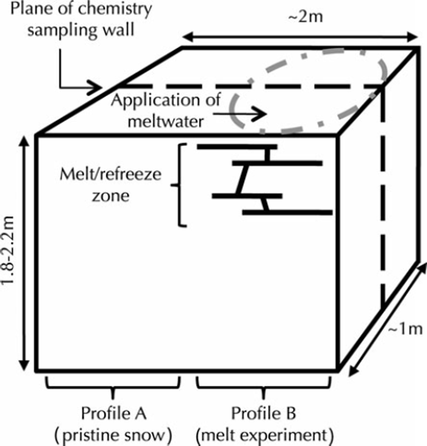
We subsequently excavated a 1.5-2.0 m deep snow pit at each experiment site, oriented such that the chemistry sampling wall was upwind and bisected the area where meltwater was applied (Fig. 1). We verified meltwater penetration by physical observation of melt features (e.g. melt fingers and ice lenses) in each snow pit. For each snow pit, we sampled two vertical profiles at 3 cm vertical resolution for chemical analysis. We positioned the profiles ∼50cm apart, such that one profile sampled snow influenced by meltwater percolation and refreeze, and the other sampled snow unaffected by meltwater penetration. Hence, we sampled a total of eight glaciochemical snow profiles, four of which were influenced by melt and four of which were not. Here, we will refer to the unaffected, pristine profile in each pit as ‘profile A’, and the meltwater-affected profile in each pit as ‘profile B’.

Fig. 1.

Perspective schematic of our experimental set-up. We applied meltwater to the surface snow. We excavated the snow pit so that the chemistry sampling wall was approximately bisecting the meltwater application area as illustrated by the dashed line. The pristine snow is represented by profile A, and the melt experiment is represented by profile B.

We sampled the snow pits for chemistry wearing non-particulating Tyvek® suits and polyethylene gloves (cf. Reference Twickler, Whitlow, Mayewski and GoodwinTwickler and Whitlow, 1997). The samples were collected in polyethylene bottles pre-cleaned with 20% nitric acid baths (cf. Reference Osterberg, Handley, Sneed, Mayewski and KreutzOsterberg and others, 2006) and stored frozen until melting prior to chemical analysis. We digitally photographed the snow-pit walls in the visible and near-infrared (850 nm) spectra, and measured snow densities at 10 cm vertical resolution for each profile in each snow pit using a 1000 cm3 cutter. Sections where melt features prevented full insertion of the density cutter were allocated the maximum density observed across the eight profiles (0.46gcm–3). We melted snow samples under a class 100 HEPA (High Efficiency Particle Air) clean bench and acidified them to 1 % by weight for a 4week period with ultrapure (Optima) nitric acid. The concentrations of trace elements were measured at the University of Maine, USA, by inductively coupled plasma sector field mass spectroscopy (ICP-SMS; Thermo Scientific Element2) (cf. Reference Osterberg, Handley, Sneed, Mayewski and KreutzOsterberg and others, 2006). We focus here on trace elements associated with insoluble dust (24Mg, 27Al, 44Ca, 47Ti, 55Mn, 56Fe, 59Co, 88Sr, 133Cs, 139La, 140Ce and 141Pr) because they exhibit a strong springtime peak representing elevated dust transport from Asia (Reference SteffensenSteffensen, 1988; Reference Whitlow, Mayewski and DibbWhitlow and others, 1992; Reference Mosher, Winkler and JaffrezoMosher and others, 1993; Reference BiscayeBiscaye and others, 1997; Reference Bory, Biscaye, Svensson and GroussetBory and others, 2002) and serve as a consistent annual marker.

Comparing snow-pit melt effect against natural variability

To isolate the effect of meltwater penetration on dust trace-element glaciochemistry against a background of natural spatial variability, three of the eight profiles were needed for each melt experiment. We compare the differences between the pristine (A) and melt-affected (B) profiles of a snow pit to the variance between that snow pit’s profile A and the nearest neighbouring snow pit’s profile A. We examine measured concentrations of elements as well as their calculated masses, based on measured concentrations and density. To exclude variability potentially caused by machine uncertainty, we first filtered the concentration data so that values below the detection limit (cf. Reference Osterberg, Handley, Sneed, Mayewski and KreutzOsterberg and others, 2006) were set to a minimum value based on laboratory blanks.

To ensure our analysis was examining snow that was deposited in the same year across all four snow pits, we applied a ‘moving window’ statistical analysis at a 50 cm stratigraphic scale. By selecting a window size that is smaller than the annual snow accumulation, we evaluated consecutive seasonal peaks independently. We incremented this analysis window down-pit by our sampling interval (3cm) to create continuous statistical analyses of dust trace elements along the entire height of the snow pits. Use of a large window overlap (i.e. 94% between adjacent windows) can allow patterns in the statistical analysis to be attributed to stratigraphic features (in contrast, applying non-overlapping window analysis does not aid in this purpose) (Reference Lutz, Birkeland, Kronholm, Hansen and AspinallLutz and others, 2007).

Here we describe the statistical procedure that was applied separately for each element measurement (concentration or mass) in each 50cm stratigraphic window. A 50 cm window contains 17 samples. First we calculate the mean difference between depth-paired measurements of adjacent A and B profiles meanB–A. This quantifies the average difference between the pristine and melt-affected profile within that stratigraphic 3 cm interval. Then the natural variability unat of the same stratigraphic interval is estimated from the variance of the differences between depth-paired measurements of the nearest pristine profile (10m away). Lastly, to determine if the meltwater treatment has an effect that is greater than the natural variability, a Student’s t test is performed to estimate the likelihood that meanB–A could have occurred by chance when the population variance is equal to unat.

Ideally unat is estimated from paired pristine profiles that are separated by the same distance as the paired profiles in the meltwater comparison. Assuming that natural variability increases with distance, our 10 m scale estimates of unat are likely larger than the natural variability occurring at adjacent profiles (0.5 m) scale. Hence we likely overestimate unat and thereby cause the t test to conservatively reject possible meltwater effects as natural variability.

Physical snowpack changes resulting from melt percolation

Visual observations (field observations and qualitative interpretation of imagery) and the physical sampling process revealed that the four snow pits show variability in the vertical distribution, thickness and patterns of ice layers and vertical ice pipes representing refrozen meltwater (Fig. 2). The melt experiment in pits 2–4 produced observable melt features extending below 3 cm depth (Figs 2 and 3), whereas in pit 1 observable melt features were limited to the upper 3 cm. Horizontal ice lenses and vertical ice fingers are both present in pits 2 and 3, with observed meltwater penetration reaching depths of 66 and 141 cm, respectively. Conversely, pit 4 developed a shallow concentration of refrozen melt-water and horizontal ice lenses between 6 and 21 cm with no visible vertical ice fingers.

Fig. 2.

Summary representation showing the stratigraphic results of the four melt percolation experiments. Melt and refreeze effects were observed in the top few centimetres of all four snow pits. Pits 2 and 3 exhibited meltwater infiltration via vertical flow fingers, which brought meltwater to greater depths below the surface than observed in pit 1 or 4. Pit 4 appeared to experience more vertical penetration of meltwater than pit 1; observed refreeze was horizontal and close to the surface.

Fig. 3.

Processed near-infrared images of meltwater penetration and refreeze formed in pits 3 and 4 at Summit Camp. While both snow pits received the same meltwater treatment, pit 4 was excavated a month after meltwater application. Dark areas indicate zones of meltwater percolation and refreeze. Also visible are many of the stratigraphic layers present in the snow pits. Images are adjusted for ambient lighting variations and scaled to Spectralon calibration targets.

Another method of determining where meltwater may have migrated within the snowpack is to compare density profiles of pristine and melt-affected snow. The average densities of profiles A and B were very similar, with the melt-affected profiles an average of 0.01–0.02 gcm–3 denser than the pristine profiles (Fig. 4), due to the addition of 15 L of meltwater. Discrete ice layers were difficult to measure accurately with the snow density cutters, introducing 20– 30% error to the density measurements. Except for the thick packet of ice lenses in pit 4, melt layers were typically much smaller than our 10cm snow cutter and heterogeneously distributed (e.g. melt fingers of pits 2 and 3).

Fig. 4.

Density (gcm–3) versus depth for each profile (A and B) in each snow pit. Pristine snow (profile A) is in solid black, and melt-affected snow (profile B) is in grey. Intervals along profile B where melt features prevented full insertion of the density cutter were approximated (see Methods), and these are shown with dashed grey boxes. The fifth column plots mean densities (gcm-3) derived from the four pristine snow-pit profiles (A) versus depth. Symbols mark profile B samples that depart from the mean density of four A profiles beyond the 95% confidence interval. The grouping of significant density changes in the top 25 cm of pits 2-4 suggests a similar pattern of meltwater penetration. Pit 4 has another interval of significant density change at ∼75 cm depth.

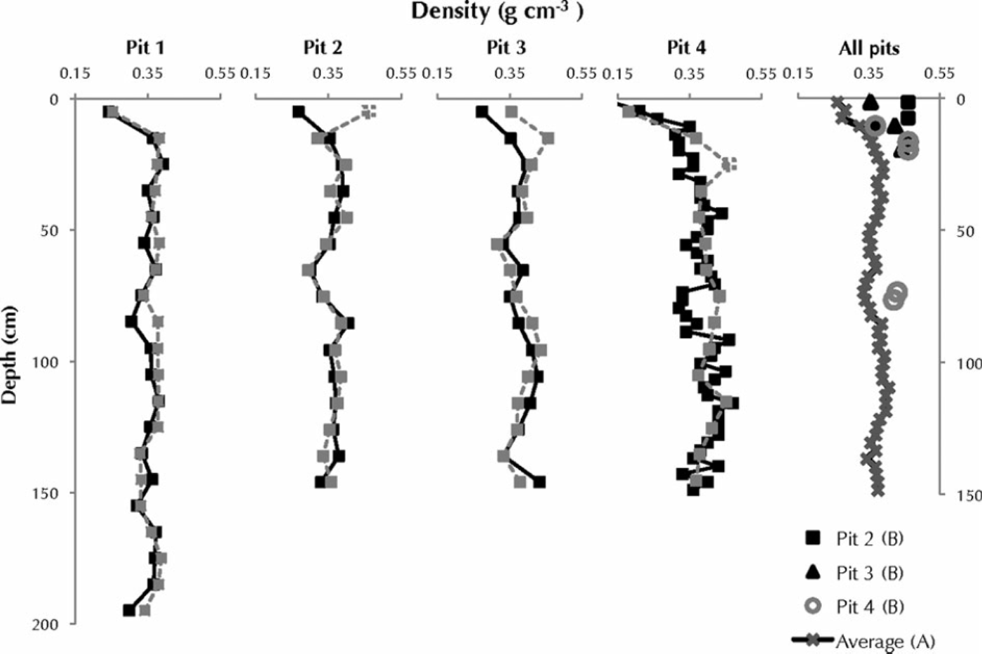
We determined the depths at which significant density changes occurred by comparing the densities from profile B of each snow pit to the average densities derived from the four A profiles. Density intervals in a profile B were considered significantly different if they were greater than the 95% confidence limit about the mean density of the four A profiles at the same depth (Fig. 4). Assuming significant changes in density were a result of meltwater intrusion and not natural variability, we can identify areas of the near-surface snowpack that have undergone densification via meltwater refreezing. Increases in density ranged between 13% and 74%; however, this includes a density interval from pit 2 that could not be directly sampled in the field due to thick melt features. The density assigned to this interval was the highest measured density across the four snow pits (0.46g cm–3). Removing this density interval reduces the densification factor to 13–34%.

Chemical snowpack changes resulting from melt percolation

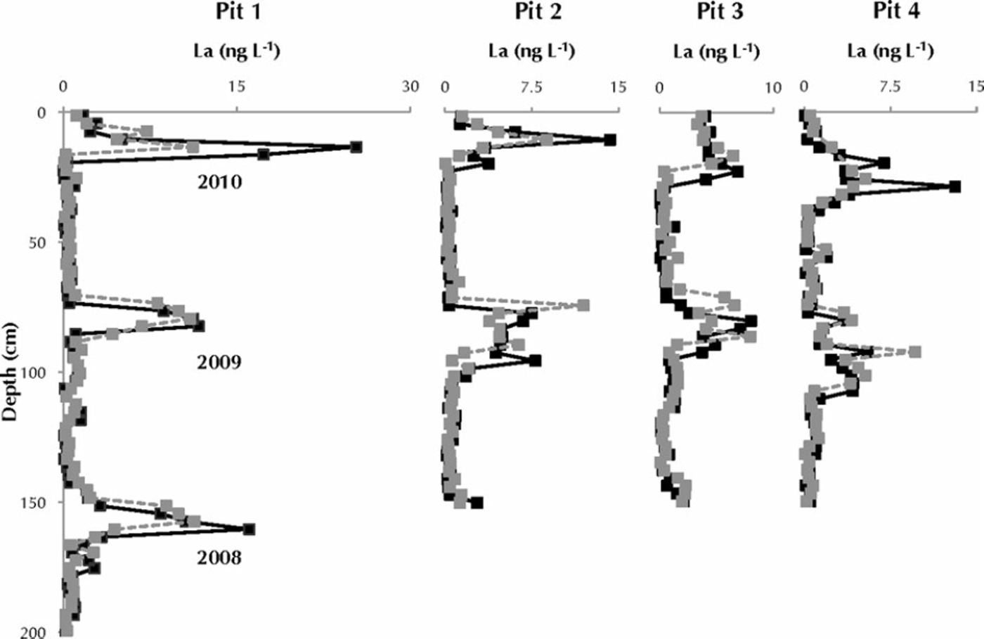
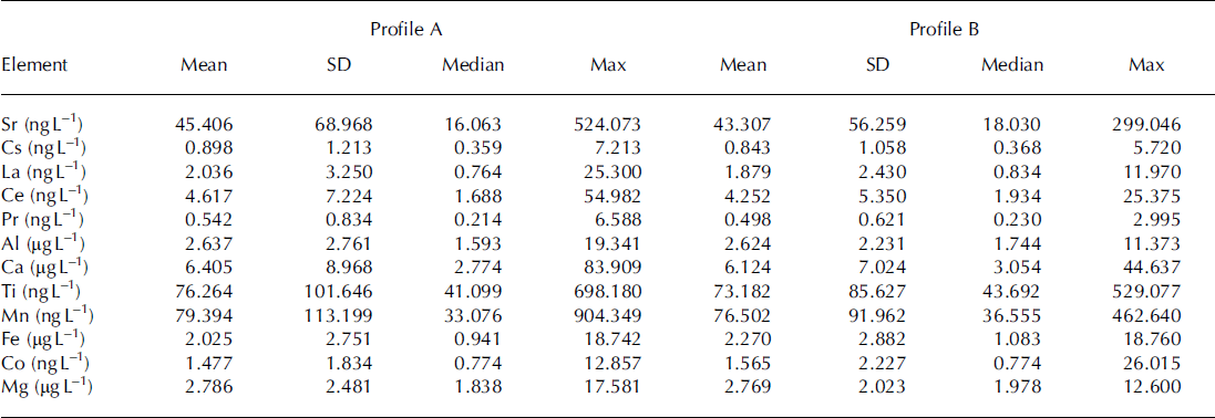
All eight chemistry profiles exhibit a strong seasonality, with annual trace-element peaks corresponding to the springtime peak in Asian dust deposition (Reference Drab, Gaudichet, Jaffrezo and ColinDrab and others, 2002). Averaged over the entire depth of the snow pits, the elemental concentrations in pristine snow are greater and more variable than in melt-affected snow, with the exception of 56Fe and 59Co (Table 1). To examine the effect of melt percolation of snow chemistry in more detail, we compare melt-affected and pristine chemical concentrations in 50 cm moving windows and focus on the springtime dust peaks in 2010 and 2009. In all four snow pits, most trace elements in the melt-affected profiles show lower (by 1–48%) spring 2010 peak concentrations and higher (by 1–47%) spring 2009 peak concentrations than in their paired pristine profiles. For example, spring 2010 peak concentrations of 88Sr in all four snow pits are diminished by 11–47% in the melt-affected profiles (Fig. 5). Conversely, spring 2009 peak concentrations of 88Sr are enriched by 1–32% in the melt-affected profiles. This behaviour reflecting melt-induced transport from the 2010 spring dust peak to lower depths in the snowpack (the 2009 annual layer) is consistently observed for each element in each snow pit with a few exceptions. For example, 44Ca, 55Mn and 59Co in the melt-affected profile of pit 4 shows enrichment in both springtime peaks (0-14%), despite showing depleted melt-affected 2010 peaks in pits 1-3. Similarly, 133Cs, 139La, 140Ce, 141Pr, 27Al, 47Ti, 55Mn, 56Fe and 59Co 2009 peak concentrations were diminished by 2-11% in pit 2, despite enrichment in the other pits. 56Fe in pit 4 shows a much larger (113%) enrichment of the 2010 springtime peak, which appears to be due to contamination from the meltwater applicator. For each element analysed, the changes in calculated mass are similar to changes in measured concentration described above.

Fig. 5.

Lanthanum concentration (ng L–1) versus depth for each profile in each snow pit. La is displayed because it behaved consistently in this series of experiments. Profile A is solid black, and profile B is grey. All eight profiles exhibit the strong seasonality of dust deposition at Summit, with springtime peaks from Asian dust influx and relatively low concentrations throughout the rest of the year (Reference Whitlow, Mayewski and DibbWhitlow and others, 1992; Reference BiscayeBiscaye and others, 1997; Reference Bory, Biscaye, Svensson and GroussetBory and others, 2002). Each spring peak is labeled by the year in which it fell.

Table 1.

The main statistics of the trace-element concentrations measured in our four snow pits split into groupings of pristine snow (profile A) and meltwater-treated snow (profile B). The distribution of means and maximum values for profile A are statistically different from those in profile B (p-value of 0.038 at a = 0.05). Except for Fe and Co, the average decrease in mean concentration for the four snow pits was 0.49-8.05%. Seasonal peak concentrations were greater in 2010 than in 2009, and the systematic diminution of average and maximum concentration values suggests a melt effect whereby meltwater intrusion removes trace elements from the 2010 peak and redistributes them in the depth interval between the 2010 and 2009 seasonal peaks

Natural spatial variability of snow chemistry versus melt-induced chemistry changes

To incorporate the natural variability of trace-element snow chemistry at Summit into the analysis of melt effects, we compare chemistry changes in melt-affected snow to the calculated variance between nearest-neighbour pristine snow profiles. This places any calculated difference between pristine and treated snow into the context of 10m scale variability. Strong seasonal variations in trace-element concentrations (masses) are present in both profiles A and B in every snow pit. Some seasonal signals show a ∼3cm vertical offset in pristine profile A compared with the adjacent, melt-affected profile B. This apparent retrograde motion of peak centres could be either a manifestation of efficient transport of material down-pit or an artefact of possible sampling offset. Therefore, we calculate and plot lagged comparisons between profiles A and B, with seasonal signals in adjacent profiles nominally centred on peak values (Fig. 6). This conservative approach addresses possible sampling errors and focuses the significance testing to distinguish between variations in seasonal deposition and meltwater transport.

Fig. 6.

Mean differences of paired pristine and melt-affected profiles, derived using 50 cm moving windows. Points along each profile mark locations where a t-test procedure identified these mean differences to be significantly larger than the natural variance estimated from the same stratigraphic segment of the two nearest pristine profiles (at the 95% confidence level). (a) Mean differences in concentrations for the four snow pits. The left column displays the mean difference of profile A from profile B (by element) for each pit, and the right column displays the number of elements demonstrating a statistically significant difference for each step of the analysis window. (b) Mean differences between calculated masses for the four snow pits, with the columns displaying similar information to that in (a). Typically, a significant difference between concentrations corresponds to a significant difference between masses, though that is not always the case (e.g. pit 4).

Our results indicate a consistent pattern across the four snow pits: as depth increases, the sign of the difference in adjacent profiles (B minus A) transitions from negative to positive (Fig. 6). Depletion of mass and diminution of concentrations in the melt-affected profiles occur in the upper third of the snow pit (Fig. 6). As the centre of the analysis window moves down-pit to the middle third of a snow pit (∼50 cm; just below the 2010 springtime peak), the sign of the difference becomes positive, indicating an addition of mass and increase in concentrations in the melt-affected profile relative to the pristine profile. The signs of the differences near the bottom third of a snow pit imply neither addition nor removal of mass. Direction of mass transport can be deduced from the sign of the difference between profiles A and B (Fig. 6). Note that while the frequency of significant differences in pits 2-4 decreases when the more conservative analysis is employed, the sign and stratigraphic location of the remaining occurrences agree with the non-lagged analysis.

Analogous to our comparison of density changes to identify zones of potential meltwater-induced mass movement, we use significant differences in concentrations (or masses) between profiles in a single snow pit to locate areas where meltwater migration vertically transported trace elements. Figure 6 shows depth ranges where the trace elements demonstrate significant melt-affected behaviour. Pits 1-3 demonstrate significant changes within 50 cm analysis windows effectively centred about ∼53 cm depth, which includes samples between 25 and 80 cm. Pit 4, which was sampled 33 days after the first three snow pits, exhibits similar behaviour centred about ∼72cm depth, which includes samples between 40 and 100 cm.

Comparing physical snowpack changes with changes in snow chemistry

Changes in trace-element distribution attributed to melt-water mobilization correspond to measured density changes and visually observed areas of refreezing. Both the observed melt features and the significant changes in measured density indicate that the top 25 cm of pits 2-4 experienced significant meltwater intrusion and refreezing. One depth where a significant density difference is located in an area with no observed melt features is 75 cm in pit 4. We measured a density in profile B that was significantly different from the mean of A profiles, but did not see evidence of melt intrusion on the snow-pit wall (Fig. 2). Similarly, differences in trace-element chemistry identify a 50 cm wide window, effectively centred at ∼ 5 3 cm depth, where it is likely meltwater has percolated through. Physical observations of pits 2-4 agree, but physical observations do not capture the potential melt-affected snow in pit 1. Here no melt features were observed below 3 cm despite the signature of melt found in the trace-element chemistry. The most inclusive measure of melt presence in the near-surface snow is the change observed in the trace-element chemistry of melt-affected snow.

Physical snowpack changes resulting from melt percolation

We observed preferential meltwater percolation in the vertical direction in addition to horizontal flow in all four snow pits (Reference Marsh Pand WooMarsh and Woo, 1984; Reference Bøggild, Forsberg and ReehBøggild and others, 2005; Reference Das and AlleyDas and Alley, 2005). Despite constraining our study to one location (Summit, Greenland), melt features presented themselves dissimilarly across the four snow pits. Vertical ice fingers reached depths of 75 and 135 cm in pits 2 and 3, respectively. Less vertical transport is observed in pits 1 and 4. There was evidence of refreeze in the top 3 cm of pit 1 and there was horizontal refreeze present between 6 and 24 cm in pit 4. Meltwater perturbation to snowpack physical and chemical properties in this study has been observed to be heterogeneous.

We observed consequent density changes with the presence of melt features, but accurately resolving all density changes resulting from refrozen meltwater is challenging. We were unable to sample density in some areas of thickly refrozen meltwater in pits 2 and 4. Additionally, vertical meltwater flow penetrated the snow-pack more deeply in pits 2 and 3 (Fig. 2) than their respective deepest significant density change. This suggests our density sampling resolution under-sampled melt-affected areas. Meltwater may have percolated down to ∼-150cm depth in all four snow pits, as it did in pit 3. An addition of 15 L of meltwater distributed evenly over the depth of each snow pit (∼150 cm) would amount to a mean density increase of 0.01 gcm–3, which is smaller than the pre-existing variations in density.

Snow chemistry changes due to natural variability and melt

Major factors influencing chemical concentrations in snow on polar ice sheets include distance inland, elevation and snow accumulation rate (Reference Mulvaney and WolffMulvaney and Wolff, 1994; Reference Yang, Mayewski, Linder, Whitlow and TwicklerYang and others, 1996). Secondary factors such as seasonality of deposition and surface roughness contribute to a lesser degree. We minimize the effects of the major factors by focusing on snow-pit chemistry changes at the 10 m scale. At Summit, Greenland, Reference Albert and HawleyAlbert and Hawley (2002) observed surface roughness amplitudes of 3-8 cm for most of the year, with a late-winter increase to 20cm. Reference Fisher, Reeh and ClausenFisher and others (1985) have modelled how increased surface roughness at a site increases the deviations in measured accumulation between two adjacent points. The surface roughness seen at Summit may explain the large difference in peak concentrations and total mass of elements between pit 1 and the other snow pits. Extending this modelled signal variance, which incorporates measured deviations in accumulation, to measured snow chemistry must account for post-depos-itional processes.

Performing intra-pit comparisons between profiles only 50cm apart diminishes the influence of variable surface roughness and increases the likelihood that the difference between any two samples or subsets of samples reflects actual chemistry changes resulting from meltwater percolation and refreeze. A moving 50 cm vertical analysis window helps further smooth potential variability. However, any analysis that depends on depth-paired samples is sensitive to small depth variations in seasonal peaks of element concentration or mass. The apparent ∼3 cm offset seen in heights between paired profiles would produce such an edge effect. If we assume the apparent ∼ 3 cm offset is due to sampling error and not due to meltwater mass transport, which may or may not be the case, we can eliminate the offset by lagging one series to reduce this edge effect. Comparing the results between unlagged and lagged differences indicates the apparent offset is not a factor in all snow pits, and that pits 2–4 show true mass transport from one seasonal peak to the previous year’s seasonal peak.

We interpret significant snow chemistry differences in the snow pits to be melt-caused, and these differences do not always coincide with physically observable melt features. Changes in chemistry due to melt percolation and refreezing were identified based on the variance defined by nearest-neighbour pairs. Chemically determined depths of melt intrusion appear to be more inclusive than the physical observations and digital imagery. This could reflect the heterogeneity of meltwater percolation and how water may intrude into spaces just behind a snow-pit wall. While there is no visual evidence of melt modification, the chemistry is sensitive to meltwater presence. Previous laboratory studies demonstrated an enrichment of filtered trace elements in the early fraction of snowmelt (Reference Abrahams, Tranter, Davies, Blackwood and LandsbergerAbrahams and others, 1988), and Reference Waldner, Schneebeli, Schultze-Zimmermann and FluhlerWaldner and others (2004) describe a flow regime (matrix flow) where the transition from a pendular liquid phase arrangement to a funicular arrangement does not visually manifest itself with macroscopic heterogeneities. Movement of meltwater in the microstructure, while potentially enriched in trace elements, may not be visible in the macroscale. Physical effects of melt were not always observed in conjunction with melt-affected snow chemistry. Studies of melt-prone glaciers may not fully account for melt if the only tools used to determine melt presence are comparisons of observed physical characteristics. This suggests connecting higher-resolution density measurements with improved analytical chemistry techniques to more accurately determine the melt history of a site.

The large window overlap of our statistical analysis aids in determining the ‘sign’ of mass movement. Negative differences between profiles A and B suggest mass has been removed from profile B at the indicated depth(s) and is being eluted down-pit. Positive differences indicate the depths where mobile elements are settling via meltwater refreezing. This pattern of negative differences near the top of our snow pits and positive differences in the middle of our snow pits, when coupled with the physical observations of the snow pits, is more diagnostic of melt effect in near-surface snow than either measurement on its own.

Effect of melt percolation on dust trace elements

Despite the application of 15 L of meltwater, equivalent to an approximate melt index of 10%, seasonal stratigraphic peaks of dust trace elements remain roughly in place and clearly evident. Our data indicate transport of mass is most significant in the depth range between the 2010 and 2009 springtime dust aerosol peaks, or in snow that had fallen the previous summer and winter. Diminution of trace-element concentrations (e.g. 19–47% in 139La) still allows for snow chemistry peak identification in our experiments due to relatively low summer–fall background concentrations at Summit. Thus, consistent seasonal phenomena make trace elements an excellent parameter to use in dating ice cores, even in the presence of an artificially applied ice melt percentage of nearly 10%. Determining the effect of progressively larger volumes of meltwater in similar experiments may identify critical thresholds above which such seasonal oscillations are lost.

Much has been done investigating the origin and provenance of dust at Summit, Greenland (e.g. Reference Whitlow, Mayewski and DibbWhitlow and others, 1992; Reference BiscayeBiscaye and others, 1997; Reference Drab, Gaudichet, Jaffrezo and ColinDrab and others, 2002), since insoluble particles can serve as tracers for atmospheric turbidity. Our data suggest that certain elements of dust can serve as tracers for meltwater percolation. In our four melt experiments, certain trace elements (e.g. 88Sr, 139La, 140Ce, 141Pr, 47Ti) demonstrated lower mobility (i.e., showing fewer statistically significant differences between profiles A and B), while others (e.g. 44Ca and 24Mg) exhibited higher mobility. The behaviour of 139La, 140Ce and 141Pr suggests that the limited mobility of rare earth elements (REEs) within the snowpack, even in the presence of meltwater, would make them ideal reference elements to evaluate melt proportion. Similar to the use of Na+ and Mg2+ in indicating melt in other Arctic ice cores (e.g. Reference Iizuka, Igarashi, Kamiyama, Motoyama and WatanabeIizuka and others, 2002; Reference VirkkunenVirkkunen and others, 2007), REEs in comparison with the more mobile 44Ca or 24Mg may serve as melt indicators. As there are currently limited REE data from melt-affected regions, more trace-element characterizations of firn and ice cores drilled in melt-prone areas may elucidate this preferential mobilization.

Most ice cores collected on small glaciers and ice caps outside Greenland and Antarctica are affected by melt, and understanding the impact of melt percolation on trace-element chemistry becomes critical when those elements are used in proxies without regard to their potential mobility. This specifically has implications for how the trace-element budget of an ice core is affected by meltwater percolation. Most trace elements measured are associated with mineral dusts, as in the case of 139La, which are not soluble in water. Moreover, as we are leaching each melted sample in a dilute acid solution, the measured trace-element concentrations likely contain only partial mineral dust dissolution from mostly oxides and sheet silicates (Reference Osterberg, Handley, Sneed, Mayewski and KreutzOsterberg and others, 2006; Reference Rhodes, Baker, Millet and BertlerRhodes and others, 2011). Our data, while representative of the mineral dust concentration in our snow samples, are not meant to construct meaningful crustal enrichment factor values without some assessment of the degree of uncertainty associated with incongruent microparticle leaching. This determination is beyond the scope of this study.

Our data show how surface melt can significantly perturb the trace-element snow chemistry. Seasonal changes are still present in our melt experiments, but chemistry peaks may move relative to where they were initially deposited. Severe melt events can affect estimates of accumulation rates if relatively mobile trace elements (e.g. 44Ca) are used as a reference element. Reference KoernerKoerner (1977) and Reference SteffensenSteffensen (1985) discuss microparticle migration and possible size fractionation in the presence of melt. Smaller microparticles made mobile by meltwater would effectively shift seasonal peaks in measured concentrations down-pit relative to a hypothetical snowpack with no melt. Similarly, Reference Waldner, Schneebeli, Schultze-Zimmermann and FluhlerWaldner and others (2004) relate solute transport efficiency to micro-structure, noting how the boundary between a fine- and a coarse-textured snow layer acts as a barrier for meltwater. Seasonal differences in average grain size across the depth interval containing the 2009 chemistry peak may explain why mass movement became less significant beyond the 2009 spring dust peak. One possibility is the coarse, 2009 summer grains act as a capillary boundary, impeding further down-pit movement of mobilized microparticles. Micro-particles that were mobilized by percolating meltwater would collect at such transitions and make their 2009 seasonal trace-element chemistry peaks appear to occur later relative to less mobile trace elements. Quantifying microparticle densities and size distributions to investigate this is beyond the scope of this paper.

Summit study site compared to melt-prone Arctic sites

It is informative to see how our study area at Summit, Greenland, compares with other Arctic research sites that experience melt. Most ice cores extracted from the Arctic exhibit an ice column comprising 50% or more of bubble-free ice formed by melt, infiltration and refreezing (Reference KoernerKoerner, 1997). Assuming meltwater refreezes within its originating annual layer, a melt index of 50% indicates an average melt of 33% of the annual accumulation. Warmer glaciers (e.g. Austfonna, Svalbard) could see effective percolation depths beyond an annual layer (Reference Iizuka, Igarashi, Kamiyama, Motoyama and WatanabeIizuka and others, 2002). Our study site (10% melt percentage of annual accumulation; 1 1 % melt index) falls within a range defined by many well-characterized, melt-prone Arctic ice-core sites: Agassiz Ice Cap, Canada, 3%; Penny Ice Cap ∼40%; Lomonosovfonna, Svalbard, 3050%; and Austofonna 67% (Reference KoernerKoerner, 1997; Reference Goto-Azuma, Koerner and FisherGoto-Azuma and others, 2002; Reference PohjolaPohjola and others, 2002; Reference VirkkunenVirkkunen and others, 2007). Summit’s accumulation rate (24.0 cm w.e. a-1) is within the range of these Arctic sites: Agassiz Ice Cap, 15 cm w.e. a- 1 ; Penny Ice Cap, 33 cm w.e. a- 1 ; Lomonosovfonna, 36 cm w.e. a-1; and Austofonna, 50-60 cm w.e. a-1 (Reference Goto-Azuma and KoernerGoto-Azuma and Koerner, 2001; Reference Iizuka, Igarashi, Kamiyama, Motoyama and WatanabeIizuka and others, 2002; Reference PohjolaPohjola and others, 2002). Summit’s mean temperature (-328C) is the coldest of these Arctic sites: Agassiz Ice Cap, -24.58C; Penny Ice Cap, -16.68C; Lomonosovfonna, -12.58C (Reference Goto-Azuma and KoernerGoto-Azuma and Koerner, 2001; Reference PohjolaPohjola and others, 2002).

An obvious question is the degree to which our results from artificial melt experiments at Summit are applicable to glaciers with natural melt and different mean annual temperatures or accumulation. The parameter that is least like other melt-prone Arctic sites is Summit’s low mean annual temperature. Our experiments demonstrate artificial meltwater penetration into the 2009 annual layer despite the inherently cold snowpack. Higher mean annual temperatures at other glaciers imply a warmer snowpack, which increases the likelihood of surface-borne meltwater percolating down beyond just one annual layer. While these vertical conduits promote downward transport of soluble elements, thereby diminishing retention of major-ion seasonality, insoluble mobility would be more limited based on microparticle size, snow microstructure and seasonal snowpack temperature gradient. Even in study areas with large melt indices and small near-surface temperature gradients based on warm mean annual temperatures, it is unlikely that particle-bound trace elements will become highly mobilized. Despite the large difference in mean annual temperatures, our observation of limited mobility in insoluble trace elements will likely be reflected in warmer, more melt-prone ice-core sites. Thus, Arctic sites with high melt indices (e.g. Penny Ice Cap and Svalbard) could preserve seasonality in dust-derived trace elements, though melt indices greater than 50% imply both downward percolation and meltwater runoff. Mean annual accumulation and dominant aerosol source are important, with Summit considered to be a high-accumulation site with a strong seasonal dust signal. Our measurements of REEs associated with dust support our conclusion that while there is mass transport with meltwater percolation, the seasonal signal is well preserved. Coastal sites would likely need strong dust seasonality to allow interpretation of trace-element chemistry on an annual scale.