


1. Introduction
Thanks to their remarkable features such as large surface-to-volume ratio and high porosity, nanofibre webs underpin many everyday technologies, from scaffold production for tissue regeneration in tissue engineering (Barbosa et al. Reference Barbosa, Villarreal, Rodriguez, De Leon, Gilkerson and Lozano2021), drug delivery in medical technologies and nano-filtration of water and air, to sensor production (Huang et al. Reference Huang, Zhang, Kotaki and Ramakrishna2003; Nayak et al. Reference Nayak, Padhye, Kyratzis, Truong and Arnold2011; Rogalski, Bastiaansen & Peijs Reference Rogalski, Bastiaansen and Peijs2017; Zhang et al. Reference Zhang, Duan, Xu and Zhang2019). The development of the recently invented centrifugal spinning (CS) methods (also known as forcespinning or rotary jet spinning), to fabricate non-woven nanofibre webs, brings important new opportunities for the mass production of nanofibres, from both polymer solutions and melts. In the CS process, jets of polymer melt or solution emerge from a rapidly rotating nozzle under the centrifugal force. As the jets evolve through the space, they stretch into very thin and long fibres, until they land on collectors where the resultant nanofibre web is assembled. However, despite its simplicity, the CS process suffers from jet instabilities which can cause the jet (throughout this work, the terms ‘fibre’ and ‘jet’ are used alternatively) to break into arrays of drops or lead to beaded fibre formation, in both of which scenarios the resultant web is considered low grade or even low quality. On the other hand, with the CS technology still being at the early development stages, several fundamental aspects of the CS process are still unknown to date, especially due to the complexity of the interconnected phenomena and the variety of competing forces involved (Noroozi & Taghavi Reference Noroozi and Taghavi2020).
Through the CS process, as the centrifugally driven jet evolves, it is influenced by a myriad of forces and phenomena, including e.g. inertial, viscous, surface tension, gravitational and centrifugal forces (Badrossamay et al. Reference Badrossamay, Mcllwee, Goss and Parker2010; Andrade et al. Reference Andrade, Santo, Costa and Lobo2017; Atıcı, Ünlü & Yanilmaz Reference Atıcı, Ünlü and Yanilmaz2021); there also exist other factors such as solvent evaporation, heat transfer effects (temperature variation) and geometrical parameters (Padron et al. Reference Padron, Fuentes, Caruntu and Lozano2013; Lai et al. Reference Lai, Wang, Liu, Li, Zhang and Chen2021). The interactions of these phenomena and forces, coupled with inherently complex viscoelastic features of the rotating fibre, may cloud our interpretation of the effects of each individual parameter on the process performance. Among the key forces and phenomena, investigating the viscoelastic properties of a rotating jet is of significance, due largely to their complex and nonlinear behaviours, which may even affect the jet dynamics in a counterintuitive way.
Although many experimental studies have been dedicated to characterizing the CS process, such as Chen et al. (Reference Chen, Wang, Lai, Zhang and Wu2021), Li et al. (Reference Li, Lu, Hou, Zhou, Wang, Zhang and Yang2020), Lu et al. (Reference Lu, Li, Zhang, Xu, Fu, Lee and Zhang2013), Ren et al. (Reference Ren, Pandit, Elkin, Denman, Cooper and Kotha2013), Weitz et al. (Reference Weitz, Harnau, Rauschenbach, Burghard and Kern2008), Mary et al. (Reference Mary, Senthilram, Suganya, Nagarajan, Venugopal, Ramakrishna and Giri Dev2013), Zhmayev et al. (Reference Zhmayev, Divvela, Ruo, Huang and Joo2015) and Ren et al. (Reference Ren, Ozisik, Kotha and Underhill2015), the experimental investigations require long-term investments of fund and time and, ultimately, they are not able to provide a rigorous prediction of the effects of key flow parameters on the resultant fibre and its web quality. On the other hand, although mathematical modelling of the CS process can provide promising insight into the process, there exist several limitations and constraints that one encounters when using mathematical modelling techniques to address thin viscous fibre flows.
There exist mainly two techniques that one can pursue to mathematically model the CS process, namely, the string models and the Cosserat rod models. At a first glance, thanks to its mathematical simplicity, it may seem straightforward/easy to use the classic string model approaches, also known as thin fibre or asymptotic models, to analyse the CS process. The string methods are based on slender body theories, providing a framework to predict the dynamic behaviour of a jet flow whose radius of curvature is large compared with its radius (see e.g. Noroozi et al. Reference Noroozi, Arne, Larson and Taghavi2020). However, the classic string models suffer from near-nozzle singularities that arise due to ignoring terms related to bending and twisting in these regions (Götz et al. Reference Götz, Klar, Unterreiter and Wegener2008; Arne et al. Reference Arne, Marheineke, Meister and Wegener2010; Noroozi et al. Reference Noroozi, Alamdari, Arne, Larson and Taghavi2017). Unless a remedy is used to overcome the near-nozzle singularities, the string models cannot be correctly applied to predict the viscous curved jet behaviours in the CS process.
During the last decade, several works have relied on the string models to investigate the impacts of different parameters in rotating jet systems, such as prilling or glass particle production processes, all sharing the same mechanism in producing micro- or nanofibres. Many studies such as Caruntu, Padron & Lozano (Reference Caruntu, Padron and Lozano2021), Shikhmurzaev & Sisoev (Reference Shikhmurzaev and Sisoev2017), Wallwork et al. (Reference Wallwork, Decent, King and Schulkes2002), Decent, King & Wallwork (Reference Decent, King and Wallwork2002), Panda (Reference Panda2006), Părău et al. (Reference Părău, Decent, Simmons, Wong and King2007) and Marheineke & Wegener (Reference Marheineke and Wegener2009) have considered the effects of gravity, surface tension and polymer solution viscosity on the jet morphology, radius and instability using the string model. Some non-Newtonian effects, such as shear thinning and viscoelastic effects, on the curved jet instability have been investigated by Uddin, Decent & Simmons (Reference Uddin, Decent and Simmons2008), Uddin & Decent (Reference Uddin and Decent2009, Reference Uddin and Decent2010), Hawkins et al. (Reference Hawkins, Gurney, Decent, Simmons and Uddin2010), Alsharif, Uddin & Afzaal (Reference Alsharif, Uddin and Afzaal2015), Alsharif & Uddin (Reference Alsharif and Uddin2015) and Marheineke et al. (Reference Marheineke, Liljegren-Sailer, Lorenz and Wegener2016). Nevertheless, a few studies have been dedicated to solving the singularity problem of the string techniques. To eliminate the near-nozzle singularity for the CS applications, Noroozi et al. (Reference Noroozi, Arne, Larson and Taghavi2020), Noroozi et al. (Reference Noroozi, Alamdari, Arne, Larson and Taghavi2017) and Taghavi & Larson (Reference Taghavi and Larson2014a,Reference Taghavi and Larsonb) have used a simple yet effective approach, known as the regularized string approach, to yield a stable solution even at regions adjacent to the nozzle.
As a promising approach, the Cosserat rod theory has been used so far with fewer limitations compared with its counterpart, i.e. the classical string model techniques, to study the CS process mathematically. In the Cosserat rod approach, the fully coupled conservation equations including mass, linear and angular momentum equations are solved (see e.g. Mahadevan & Keller Reference Mahadevan and Keller1996; Ribe Reference Ribe2004; Ribe, Habibi & Bonn Reference Ribe, Habibi and Bonn2006), avoiding singularities such as the ones observed in the classic string model; this is done via including the bending and twisting terms in the near-nozzle regions. Arne et al. (Reference Arne, Marheineke, Meister and Wegener2010) and Arne et al. (Reference Arne, Marheineke, Meister, Schiessl and Wegener2015) have used a Cosserat rod theory to model a curved jet in two-dimensional (2-D) stationary and 3-D transient frames, respectively, to study a viscous curved jet in the glass wool spinning process. In another attempt, Liu & Parker (Reference Liu and Parker2018) have developed a Cosserat beam theory to model a viscoelastic curved jet in a 2-D stationary frame, to study the CS process. However, compared with the string model, extending the rod model to include the surface forces and nonlinear viscoelastic models is more difficult and the resulting model equations are eventually more demanding to solve.
In the majority of the previous works, due to their limitations/singularities, the string model equations cannot be directly applied to study the CS process (which involves a rapidly rotating viscous flow). Therefore, in this work, we develop a rigorous mathematical model to remove the existing barriers to properly analyse the CS process. The novelties and contributions of the current work are as follows. First, when developing our mathematical model, we use the Bishop bases to define the jet baseline using its full curvature components; this enables us to develop and solve the final equations in the 2-D and 3-D spaces much easier since the jet baseline torsion is not dealt with explicitly. Second, we successfully remove the singularity problem of the classic asymptotic string equations via incorporating the angular momentum conservation equations into the model. As we consider viscoelastic slender jets, the first-order viscoelastic extra stress terms are also included into the angular momentum conservation equations; using this approach, the equations can also be easily extended in future to consider a jet with non-circular cross-sections. Furthermore, our model equations includes the Giesekus nonlinear constitutive model coupled with the energy equation, the kinematic expressions as well as the aerodynamic drag force relations; this inclusiveness, in return, allows us to predict the effects of viscoelastic, inertial, rotational, surface tension, gravitational, polymer melt/solution temperature and aerodynamic effects, on the fibre flow. Finally, we develop the model equations in their general form and in the 3-D space so that they can be easily tailored to study any spinning processes, in unsteady or in steady state conditions. Thanks to the comprehensiveness of the model developed, it is possible to explore the effects of a wide range of key dimensionless flow parameters. This makes it possible to rigorously analyse the performance of the CS process in the current work and similar processes (melt spinning, prilling, etc.) in future, for a wide range of material choices, from a Newtonian solvent to a highly viscoelastic solution to a viscoelastic polymer melt, not addressed in previous works.
The outline of the current paper is as follows. In § 2, we present the methods used to derive our mathematical model, comprising the assumptions, the governing equations, the boundary and initial conditions and finally the asymptotic method employed to simplify the resultant equations. In § 3, we first show the behaviour of a transient jet and then study parametrically the effects of various flow parameters on the steady jet dynamic behaviour. Finally in § 4, we conclude the paper with a brief summary of the main findings.
2. Problem formulation
In this work, we derive the asymptotic equations for a viscoelastic curved jet emanating from a rotating nozzle with the constant rotation speed  $\varOmega$ rad s $^{-1}$, diameter $a$ and length
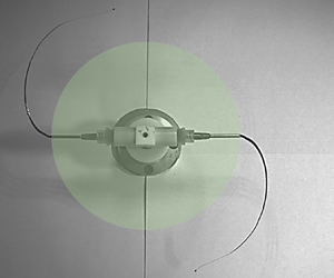
  $s_0$, as schematically shown in figure 1. Our derivation is based on the slender body approach consisting of projecting the equations in a 3-D space onto the Bishop basis vectors (Bishop Reference Bishop1975), used to eliminate the baseline torsion and accordingly ease the derivation procedure. In the next step, we use the cross-sectional averaging techniques followed by expansions of cross-averaged variables based on the slenderness parameter, i.e. the aspect ratio $\varepsilon =a/s_0$, to derive our set of asymptotic equations. Finally, we solve the leading-order equations in $\varepsilon$ with the aid of numerical approaches.
Left image: a schematic view of a typical laboratory scale CS process. The nozzle inner diameter is marked by  $a$, the spinneret radius by $s_0$ and the fibre angles by $\alpha$ and $\beta$. Right image: a segment of the jet with the reference frames. In the left and right images, we show several parameters related to the model explained in the model section; $\omega _{N_1}, \omega _{N_2}, \omega _{T}$ are the components of the jet cross-section angular velocity vector.

2.1. Controlling parameters of the CS process
In the CS process, under a centrifugal force, a polymer solution or melt emerges from a nozzle of a rapidly rotating reservoir, also known as the spinneret, forming a nanosized curved jet as schematically sketched in figure 1. As the jet emerges from the nozzle (regime 1), it starts to stretch and it develops a time and position dependent trajectory and radius. However, at long times when the fibre touches the collectors, its behaviour becomes steady (regime 2) in a way that the jet trajectory does not change with time anymore, provided that there are no perturbations or jet breakups. To better visualize how the jet is initially developed and reaches the steady state, figure 2 shows the formation of a growing polymer solution jet over time, in our laboratory CS set-up, a detailed description of which can be found in Noroozi et al. (Reference Noroozi, Arne, Larson and Taghavi2020). As observed, at short times, the polymer solution is extruded into a straight jet and starts to bend in the anti-rotation direction. With increasing time, the fibre goes through a range of transient shapes, from a pedant drop, to an anti-S shape jet (Li et al. Reference Li, Lu, Hou, Zhou, Wang, Zhang and Yang2020), to a necking point, etc. Next, the fibre continues to grow until it finally reaches the steady condition where its trajectory no longer changes with time. According to the figure, one can realize that the transient part of the fibre formation in the CS process, i.e. regime 1, is very fast and it merely takes one or two spinning cycles for a growing fibre to turn into a steady jet (regime 2). Although the major part of the process occurs in regime 2, studying regime 1 is also of importance, since it will eventually make the analysis of the jet stability possible. Thus, in this work, we derive a complete set of model equations including the transient forms, to set the stage for future analysis of jet stability.
Experimental observation of a growing fibre over time in a typical CS experiment, using a poly(ethylene oxide) (PEO) solution. The field of view in all images is  $140\,{\rm mm}\times 250\,{\rm mm}$. The solution is $7\,\%$wt PEO (with the molecular weight of $M_{v}=9 \times 10^{5}$ (g mol $^{-1}$)), and the experimental parameters are $\varOmega =370$ (rad s $^{-1}$), $s_0=8$ (cm) and $a=1$ (mm). The times with respect to the beginning of the experiment are given in seconds in the corner of each image.

During jet flight time, many parameters affect the jet dynamic behaviour and, consequently, its size (radius) and shape; these parameters may include rotational (comprising centrifugal and Coriolis effects), viscoelastic, inertial, gravitational, aerodynamic (air drag), surface tension and jet temperature variation effects. In this study, the effects of these parameters will be taken into account in our model, through several dimensionless numbers as the input parameters of the model, listed in Table 1. These dimensionless numbers quantify the aforementioned phenomena and forces. In particular,  $Rb$,
$Rb$,  $Fr$,
$Fr$,  $Re$,
$Re$,  $We$,
$We$,  $Pe^*$ and $Re^*$ can be interpreted as the inverse dimensionless rotation rate, gravitational acceleration, polymer solution viscosity, surface tension, air thermal diffusivity and air viscosity, respectively, provided that the flow rate, density and geometrical parameters are constant. Also, $Wi$ is similarly a representative of the polymer solution/melt relaxation time, $\lambda$.
Definitions of the dimensionless groups along with their typical ranges in a typical CS process. The subscript ‘ $noz$’ marks the polymer solution/melt jet parameters at the nozzle exit and the dimensional and dimensionless parameters describing properties in the air are marked with an asterisk ( $*$). We also use the subscript ‘ $p$’ to mark the polymer properties and ‘ $s$’ to mark the solvent properties. Here, $\rho$ stands for the density, $U$ the velocity, $\bar {\sigma }$ the surface tension, $\mu =\mu _{s}+\mu _{p}$ the zero-shear viscosity (with $\mu _s$ and $\mu _p$ being the solvent and polymer contributions to the zero-shear viscosity, respectively), $\lambda$ the relaxation time, $\theta$ the temperature, ${c_{p}}$ the specific heat capacity, $k$ the conductivity and $\mathrm {g}$ the gravitational acceleration. In addition to the parameters presented, our steady state and transient models will respectively use $\ell =L/s_0$ and $\tau _{end}$ (the end time, made dimensionless using the characteristic time $s_0/U_{noz}$), as additional input parameters.

To preserve the generality of the results, we present all the variables and equations in their dimensionless forms throughout this study. To do so, we use the nozzle diameter ( $a$) to scale the fibre radius and we use $s_0$ as a length scale, $s_0/U_{noz}$ as the time scale, $U_{noz}$ as the velocity scale, $U_{noz}/s_0$ as the angular velocity scale, $A_{ref}={\rm \pi} a^2/4$ as the reference area, $\mu _{noz} U_{noz}/s_0$ as the stress scale and, finally, $\theta _{noz}$ as the temperature scale.
2.2. Governing equations
The CS of a viscoelastic fibre can be described using the transient three-dimensional conservation equations, along with viscoelastic constitutive equations of the polymer solution/melt. To write out the governing equations, we treat the jet as a single incompressible phase and ignore the effects of the solvent evaporation on the fibre behaviour. Therefore, the dimensionless continuity, momentum, angular momentum, energy and Giesekus viscoelastic constitutive equations can be represented respectively as
 $$\begin{gather} {\partial _t}\bar \rho + \boldsymbol{\nabla} \boldsymbol{\cdot} \left({\bar \rho {\boldsymbol{v}}}\right) = 0, \end{gather}$$
 $$\begin{gather}{\partial _t}{\boldsymbol{v}} + {\boldsymbol{v}} \boldsymbol{\cdot}\boldsymbol{\nabla} {\boldsymbol{v}} = \boldsymbol{\nabla}\boldsymbol{\cdot}{\boldsymbol{\varPi }}+{\boldsymbol{F}}, \end{gather}$$
 $$\begin{gather}{\partial _t}\left( {{\boldsymbol{d}} \times {\boldsymbol{v}}} \right) + {\boldsymbol{v}}\boldsymbol{\cdot}\boldsymbol{\nabla} \left({{\boldsymbol{d}} \times {\boldsymbol{v}}} \right) = \boldsymbol{\nabla}\boldsymbol{\cdot}\left( {{\boldsymbol{d}} \times {\boldsymbol{\varPi }}} \right) + {\boldsymbol{d}} \times {\boldsymbol{F}}, \end{gather}$$
 $$\begin{gather}{\partial _t}\theta + {\boldsymbol{v}}\boldsymbol{\cdot}\boldsymbol{\nabla} \theta = \frac{1}{{Pe}}{\nabla^2}\theta, \end{gather}$$
 $$\begin{gather}\bar{\lambda}Wi\left( {{\partial _t}{\boldsymbol{\mathsf{S}}} + {\boldsymbol{v}}\boldsymbol{\cdot}\boldsymbol{\nabla}{\boldsymbol{\mathsf{S}}} - \left({{\boldsymbol{\mathsf{S}}}\boldsymbol{\cdot}\boldsymbol{\nabla} {\boldsymbol{v}} + {{\left( {\boldsymbol{\nabla} {\boldsymbol{v}}} \right)}^{\rm T}}\boldsymbol{\cdot}{\boldsymbol{\mathsf{S}}}} \right)}\right) + \left({\frac{{\bar{\lambda} Wi\chi }}{{(1 - {\delta _s})}}{\boldsymbol{\mathsf{S}}} + {\boldsymbol{I}}} \right)\boldsymbol{\cdot}{\boldsymbol{\mathsf{S}}} = 2(1 - {\delta _s}){\boldsymbol{\gamma }}, \end{gather}$$
in which  $\boldsymbol {v}$ denotes the velocity vector, $\bar {\rho }=\rho (\theta )/\rho _{noz}$ the relative density, $\boldsymbol {d}$ the position vector, $\boldsymbol {\varPi }$ the stress tensor (yet to be determined), $\boldsymbol{\mathsf{S}}$ the extra stress tensor related to viscoelasticity, $\theta$ the dimensionless jet temperature, $\boldsymbol {\gamma }$ the strain rate tensor, $\chi$ the mobility factor, $\bar {\lambda }=\lambda (\theta )/\lambda _{noz}$ the relative relaxation time, $\delta _s$ the viscosity ratio; also, $\bar {\mu }=\mu _p(\theta )/\mu _{pnoz}$ stands for the relative polymer zero-shear viscosity; see table 1 for the definitions of the dimensionless numbers. We also define $Wi=\lambda _{noz} U_{noz}/s_0$ in which $\lambda _{noz}$ is the polymer relaxation time at the nozzle. Finally, $\boldsymbol {F}$ stands for the external force vectors consisting of the Coriolis, centrifugal, gravitational and drag forces, defined as
 \begin{equation} {\boldsymbol{F}} ={-} \frac{2}{{Rb}}{\boldsymbol{\varOmega }} \times {\boldsymbol{v}} - \frac{1}{{R{b^2}}}{\boldsymbol{\varOmega }} \times \left( {{\boldsymbol{\varOmega }} \times {\boldsymbol{d}}} \right)+\frac{{\boldsymbol{g}}}{{F{r^2}}} + {{\boldsymbol{F}}_{{drag}}}, \end{equation}
where  $\boldsymbol {\varOmega }=(1,0,0)$ denotes the angular velocity vector, $\boldsymbol {g}=(-1,0,0)$ is the gravity acceleration vector and $\boldsymbol {F}_{{drag}}$ stands for the aerodynamic drag force vector, yet to be defined. Solving the full 3-D set of equations coupled with the viscoelastic constitutive relations and the boundary conditions at the jet free surface (to be defined) is not feasible, in a transient or even stationary frame. Therefore, in this work, we define the variables based on the cross-averaged values in the axial direction and then develop a set of quasi-1-D equations using the asymptotic estimations of the key parameters. Prior to deriving the governing equations, however, we need to define some geometrical and kinematic relations to frame an unsteady viscoelastic curved jet, presented in the following.
2.3. Coordinate systems and basis vectors
In this section, we introduce the coordinate systems and their corresponding bases to frame our unsteady curved jet. To this aim, we use 3-tuple  $(n_1, n_2, s)$ as our curvilinear coordinate system so that $s$ defines the arc length and $(n_1, n_2)$ defines the jet cross-section as rectangular coordinates normal to the jet baseline. When defining the jet cross-section, we can also find it helpful to use polar coordinates $(r, \varphi )$ whose relations with $(n_1, n_2)$ are
 \begin{equation} \left.\begin{gathered} r = \sqrt {n_1^2 + n_2^2},\quad \varphi = {\tan ^{ - 1}} \left( {\frac{{{n_1}}}{{{n_2}}}} \right),\quad \text{or} \\ {n_1} = r\sin (\varphi ),\quad {n_2} = r\cos (\varphi). \end{gathered}\right\} \end{equation}
In this study, whenever more appropriate, we use the polar coordinates to describe the jet cross-section using back-and-forth transformation relations expressed in (2.7).
Next, we present the basis vector expressions to define the baseline of the jet. We choose the Cartesian coordinate system as an outer frame to define the jet baseline, so that the nozzle, from which the jet emerges, is fixed. Given this, we can introduce a time-dependent three-dimensional curve function
 \begin{equation} \boldsymbol{D}(s,t)= X(s,t)\boldsymbol{\hat x } + Y(s,t)\boldsymbol{\hat y} + Z(s,t)\boldsymbol{\hat z}, \end{equation}
as the jet baseline position in which  $t$ is time and $(\boldsymbol {\hat x}, \boldsymbol {\hat y}, \boldsymbol {\hat z})$ are the Cartesian basis vectors. We also use the Bishop basis vectors $(\boldsymbol {N_1}, \boldsymbol {N_2}, \boldsymbol {T})$, which are orthonormal, as the moving frame of reference for our curved jet centreline and derive the final uniaxial equations. In this work, we use the Bishop basis vectors instead of the commonly used Frenet basis vectors to frame our curved baseline for two reasons: first, we would like to exclude the baseline torsion from our calculation when deriving our set of equations and, second, we would like to ease the cumbersome derivation procedure of the governing equations in the previous works in this area; see for instance Noroozi et al. (Reference Noroozi, Arne, Larson and Taghavi2020) or Shikhmurzaev & Sisoev (Reference Shikhmurzaev and Sisoev2017). Furthermore, to simplify the basis vector derivatives with respect to time and space and also the kinematic expressions (yet to be introduced), it may be a good idea to use the fibre angles ( $\alpha, \beta$; see figure 1), to compute the baseline function derivatives as
 \begin{equation} \left.\begin{gathered} {X_{,s}} = \cos (\beta),\\ {Y_{,s}} = \cos (\alpha )\sin (\beta),\\ {Z_{,s}} = \sin (\alpha )\sin (\beta), \end{gathered}\right\} \end{equation}
which automatically satisfy the arc length condition expressed as
 \begin{equation} X_{,s}^2 + Y_{,s}^2 + Z_{,s}^2 = 1. \end{equation}
It is noted that, herein, for convenience we use  $H_{,s}$ or $H_{,t}$ as the partial derivative of an arbitrary function $H(s, t)$ with respect to $s$ or $t$. We also define ${\langle {H} \rangle _T}$ as the projection of a given vector $\boldsymbol {H}$ onto an arbitrary base vector such as $\boldsymbol {T}$. We further introduce the baseline curvature components, i.e. $\kappa _i,\ i=1, 2, 3$, determined as
 \begin{equation} {\kappa _1} = {\beta _{,s}},\quad {\kappa _2} = {\alpha _{,s}}\sin (\beta ),\quad {\kappa _3} = {\alpha _{,s}}\cos (\beta ). \end{equation}
The two former components are also known as the Bishop curvatures. Using (2.11a–c) the baseline curvature  $\kappa$ and torsion $\mathcal {T}$ can be obtained as
 $$\begin{gather} \kappa= \sqrt {\kappa _1^2 + \kappa _2^2}, \end{gather}$$
 $$\begin{gather}\mathcal{T} = {\kappa _3} + {\left| \kappa \right|^{ - 2}} \left( {{\kappa _1}{\kappa _{2,s}} - {\kappa _2}{\kappa _{1,s}}} \right). \end{gather}$$
Now, using the aforementioned expressions, we can define the Bishop basis vectors  $({\boldsymbol {N}}_1, {\boldsymbol {N}}_2, \boldsymbol {T})$ as (Bishop Reference Bishop1975):
 $$\begin{gather} {{\boldsymbol{N}}_1} = {\boldsymbol{B}}\frac{{{\kappa _2}}}{\kappa } - {\boldsymbol{N}} \frac{{{\kappa _1}}}{\kappa }, \end{gather}$$
 $$\begin{gather}{{\boldsymbol{N}}_2} ={-}{\boldsymbol{B}}\frac{{{\kappa _1}}}{\kappa } - {\boldsymbol{N}} \frac{{{\kappa _2}}}{\kappa }, \end{gather}$$
 $$\begin{gather}{\boldsymbol{T}} = {\boldsymbol{T}}, \end{gather}$$
in which  $(\boldsymbol {T}, \boldsymbol {N}, \boldsymbol {B})$ are the Frenet basis vectors, i.e. the tangent, normal and binormal unit vectors, respectively, defined as
 $$\begin{gather} \boldsymbol{T} = \frac{{{\rm d}\boldsymbol{D}}}{{{\rm d} s}} = {X_{,s}}\boldsymbol{\hat x }+ {Y_{,s}}\boldsymbol{\hat y} + {Z_{,s}}\boldsymbol{\hat z}, \end{gather}$$
 $$\begin{gather}\boldsymbol{N} = \frac{{{\rm d}\boldsymbol{T}}}{{{\rm d} s}}{\left|{\frac{{{\rm d}\boldsymbol{T}}}{{{\rm d} s}}} \right|^{ - 1}} = \frac{{{X_{,ss}}\boldsymbol{\hat x} + {Y_{,ss}}\boldsymbol{\hat y } + {Z_{,ss}}\boldsymbol{\hat z }}}{{\sqrt {{{\left( {{X_{,ss}}} \right)}^2} + {{\left( {{Y_{,ss}}}\right)}^2} + {{\left( {{Z_{,ss}}} \right)}^2}} }}, \end{gather}$$
 $$\begin{gather}\boldsymbol{B} = \boldsymbol{T} \times \boldsymbol{N} = \frac{{\left({{Y_{,s}}{Z_{,ss}} - {Y_{,ss}}{Z_{,s}}} \right)\boldsymbol{\hat x } + \left( {{Z_{,s}}{X_{,ss}} - {Z_{,ss}}{X_{,s}}} \right)\boldsymbol{\hat y } + \left( {{X_{,s}}{Y_{,ss}} - {X_{,ss}}{Y_{,s}}} \right) \boldsymbol{\hat z }}}{{\sqrt {{{\left({{X_{,ss}}} \right)}^2} + {{\left( {{Y_{,ss}}} \right)}^2} + {{\left({{Z_{,ss}}} \right)}^2}} }}. \end{gather}$$
Using (2.9), (2.11a–c) and (2.14)–(2.19), we can find
 \begin{equation} \left.\begin{gathered} {{\boldsymbol{N}}_1} = \left( {\sin (\beta )} \right){\boldsymbol{\hat x}} - (\cos (\alpha )\cos (\beta )){\boldsymbol{\hat y}}- \left( {\sin (\alpha )\cos (\beta )} \right){\boldsymbol{\hat z}}, \\ {{\boldsymbol{N}}_2} = (\sin (\alpha )){\boldsymbol{\hat y}} - \left( { \cos (\alpha )} \right){\boldsymbol{\hat z}}, \\ {\boldsymbol{T}} = \left( {\cos (\beta )} \right){\boldsymbol{\hat x}}+(\cos (\alpha )\sin (\beta )){\boldsymbol{\hat y}} + \left( {\sin (\alpha )\sin (\beta )} \right){\boldsymbol{\hat z}}. \end{gathered}\right\} \end{equation}
Next, using (2.11a–c) and (2.20), the derivatives of the Bishop basis vectors can be obtained with respect to the arc length  $s$ as
 \begin{equation} \left.\begin{gathered} \frac{{\partial {{\boldsymbol{N}}_1}(s,t)}}{{\partial s}} = {\kappa _1}{\boldsymbol{T}} + {\kappa _3}{{\boldsymbol{N}}_2}, \\ \frac{{\partial {{\boldsymbol{N}}_2}(s,t)}}{{\partial s}} = {\kappa _2}{\boldsymbol{T}} - {\kappa _3}{{\boldsymbol{N}}_1}, \\ \frac{{\partial {\boldsymbol{T}}(s,t)}}{{\partial s}} ={-} {\kappa _1}{{\boldsymbol{N}}_1} - {\kappa _2}{{\boldsymbol{N}}_2}, \end{gathered}\right\} \end{equation}
and with respect to time  $t$ as
 \begin{equation} \left.\begin{gathered} \frac{{\partial {{\boldsymbol{N}}_1}(s,t)}}{{\partial t}} = \left( {{\beta _{,t}}} \right){\boldsymbol{T}} + \left( {{\alpha _{,t}}\cos (\beta )} \right){{\boldsymbol{N}}_2}, \\ \frac{{\partial {{\boldsymbol{N}}_2}(s,t)}}{{\partial t}} = \left( {{\alpha _{,t}}\sin (\beta )} \right){\boldsymbol{T}} - \left( {{\alpha _{,t}}\cos (\beta )} \right){{\boldsymbol{N}}_1}, \\ \frac{{\partial {\boldsymbol{T}}(s,t)}}{{\partial t}} ={-} \left( {{\alpha _{,t}}\sin (\beta )} \right){{\boldsymbol{N}}_2} - \left( {{\beta _{,t}}} \right){{\boldsymbol{N}}_1}. \end{gathered}\right\} \end{equation}
 Now, we turn from the baseline geometry to that of the fibre as a whole, for the definition of which we use the covariant basis vectors,  ${\boldsymbol {g}_{1}}$, ${\boldsymbol {g}_{2}}$ and ${\boldsymbol {g}_{3}}$ corresponding to $n_1$, $n_2$ and $s$ directions, respectively; see figure 1. Based on our definition here, the time-dependent position vector of an arbitrary point $\boldsymbol {d}$ inside the fibre at a given time $t$ can be expressed as
 \begin{equation} {\boldsymbol{d}}(n_1,n_2,s,t) = {\boldsymbol{D}}(s,t) + \varepsilon{n_1}{{\boldsymbol{N}}_1} + \varepsilon{n_2}{{\boldsymbol{N}}_2} = {\boldsymbol{D}}(s,t) + \varepsilon{\boldsymbol{r}}, \end{equation}
in which  $\boldsymbol {r}$ is $(n_1, n_2, 0)$, so as $| {\boldsymbol {r}} |=r$, and $\varepsilon$ is the aspect ratio. Given the position vector of an arbitrary point $\boldsymbol {d}$, i.e. (2.23), we can define the covariant basis vectors as
 \begin{equation} {{\boldsymbol{g}}_i} = \frac{{\partial {\boldsymbol{d}}}}{{\partial {s^i}}}\quad (i = 1, 2, 3)\quad {\rm{and}}\quad ({s^1} = {n_1},\ {s^2} = {n_2},\ {s^3} = s), \end{equation}
and therefore we have
 \begin{equation} \left.\begin{gathered} {{\boldsymbol{g}}_1} = \frac{{\partial {\boldsymbol{d}}}}{{\partial {n_1}}} = {\varepsilon{\boldsymbol{N}}_1},\quad {{\boldsymbol{g}}_2} = \frac{{\partial {\boldsymbol{d}}}}{{\partial {n_2}}} = {\varepsilon{\boldsymbol{N}}_2}, \\ {{\boldsymbol{g}}_3} = \frac{{\partial {\boldsymbol{d}}}}{{\partial s}} ={-} \left( {\varepsilon {n_2}{\kappa _3}} \right){{\boldsymbol{N}}_1} + \left( {\varepsilon {n_1}{\kappa _3}} \right){{\boldsymbol{N}}_2} + \left( {1 + \varepsilon {n_1}{\kappa _1} + \varepsilon {n_2}{\kappa _2}} \right){\boldsymbol{T}}. \end{gathered}\right\} \end{equation}
Thus, we can define the metric tensor as
 \begin{equation} \left.\begin{gathered}
({g_{ij}})=
{{\boldsymbol{g}}_i}\boldsymbol{\cdot}{{\boldsymbol{g}}_j}
= \begin{pmatrix} {{\varepsilon ^2}} & 0 &
{ - {\varepsilon ^2}{n_2}{\kappa _3}}\\ 0 & {{\varepsilon
^2}} & {{\varepsilon ^2}{n_1}{\kappa _3}}\\ { -
{\varepsilon ^2}{n_2}{\kappa _3}} & {{\varepsilon
^2}{n_1}{\kappa _3}} & {{h^2} + {\varepsilon ^2}{r^2}\kappa
_3^2}\end{pmatrix}, \\ \left| {{g_{ij}}}
\right| = \varepsilon^4 {h^2},\quad h = \left( {1 +
\varepsilon{n_1}{\kappa _1} + \varepsilon{n_2}{\kappa _2}}
\right), \end{gathered}\right\} \end{equation}
\begin{equation} \left.\begin{gathered}
({g_{ij}})=
{{\boldsymbol{g}}_i}\boldsymbol{\cdot}{{\boldsymbol{g}}_j}
= \begin{pmatrix} {{\varepsilon ^2}} & 0 &
{ - {\varepsilon ^2}{n_2}{\kappa _3}}\\ 0 & {{\varepsilon
^2}} & {{\varepsilon ^2}{n_1}{\kappa _3}}\\ { -
{\varepsilon ^2}{n_2}{\kappa _3}} & {{\varepsilon
^2}{n_1}{\kappa _3}} & {{h^2} + {\varepsilon ^2}{r^2}\kappa
_3^2}\end{pmatrix}, \\ \left| {{g_{ij}}}
\right| = \varepsilon^4 {h^2},\quad h = \left( {1 +
\varepsilon{n_1}{\kappa _1} + \varepsilon{n_2}{\kappa _2}}
\right), \end{gathered}\right\} \end{equation}
in which  $| {{g_{ij}}} |$ denotes the determinant of the metric tensor. As vividly seen, our local bases are neither orthogonal nor normalized due to non-zero off-diagonal elements and non-unity of the diagonal ones. Using (2.26), we can attain the conjugate metric tensor ${{g}}^{ij}$ such that
 \begin{equation} {g}^{ik}\cdot{g}_{kj}=\delta^{i}_{j}, \end{equation}
where  $\delta ^{i}_{j}$ stands for the Kronecker delta; therefore, we arrive at
 \begin{equation} ({g^{ij}}) =
\frac{{{\varepsilon ^2}}}{{\left| {{g_{ij}}} \right|}}
\begin{pmatrix} {{h^2} + {\varepsilon
^2}n_2^2\kappa _3^2} & { - {\varepsilon ^2}{n_1}{n_2}\kappa
_3^2} & {{\varepsilon ^2}{n_2}{\kappa _3}}\\ { -
{\varepsilon ^2}{n_1}{n_2}\kappa _3^2} & {{h^2} +
{\varepsilon ^2}n_1^2\kappa _3^2} & { - {\varepsilon
^2}{n_1}{\kappa _3}}\\ {{\varepsilon ^2}{n_2}{\kappa _3}} &
{ - {\varepsilon ^2}{n_1}{\kappa _3}} & {{\varepsilon ^2}} \end{pmatrix}. \end{equation}
\begin{equation} ({g^{ij}}) =
\frac{{{\varepsilon ^2}}}{{\left| {{g_{ij}}} \right|}}
\begin{pmatrix} {{h^2} + {\varepsilon
^2}n_2^2\kappa _3^2} & { - {\varepsilon ^2}{n_1}{n_2}\kappa
_3^2} & {{\varepsilon ^2}{n_2}{\kappa _3}}\\ { -
{\varepsilon ^2}{n_1}{n_2}\kappa _3^2} & {{h^2} +
{\varepsilon ^2}n_1^2\kappa _3^2} & { - {\varepsilon
^2}{n_1}{\kappa _3}}\\ {{\varepsilon ^2}{n_2}{\kappa _3}} &
{ - {\varepsilon ^2}{n_1}{\kappa _3}} & {{\varepsilon ^2}} \end{pmatrix}. \end{equation}
Using (2.25), (2.26) and (2.28), we can obtain the gradient operator in our curvilinear coordinate system as
 \begin{equation} \boldsymbol{\nabla} = {g^{ik}}{{\boldsymbol{g}}_k}\frac{\partial }{{\partial {s^i}}} = \left(\frac{1}{\varepsilon }{{\boldsymbol{N}}_1} + \frac{{{n_2}{\kappa _3}}}{h}{\boldsymbol{T}}\right) \frac{\partial }{{\partial {n_1}}} + \left(\frac{1}{\varepsilon }{{\boldsymbol{N}}_2} - \frac{{{n_1}{\kappa _3}}}{h}{\boldsymbol{T}}\right)\frac{\partial }{{\partial {n_2}}} + \left(\frac{1}{h}{\boldsymbol{T}}\right)\frac{\partial }{{\partial s}}, \end{equation}
from which we can later determine the strain rate tensor. In the next step, we derive the corresponding kinematic relations, the stress tensor and the dynamic boundary condition equations using the aforementioned expressions.
2.4. Kinematic relations
To study an unsteady growing curved jet, two kinds of velocities can be realized at each point inside the liquid jet. The first one is the fluid velocity and it can be expressed as the material derivative of the position vector  $\boldsymbol {d}$ as
 \begin{equation} {\boldsymbol{v}} = \frac{{{\rm d}{\boldsymbol{d}}(n_1, n_2, s, t)}}{{{\rm d} t}} = \frac{{\partial {\boldsymbol{d}}}}{{\partial t}} + \frac{{\partial {\boldsymbol{d}}}}{{\partial {n_1}}} \frac{{\partial {n_1}}}{{\partial t}} + \frac{{\partial {\boldsymbol{d}}}}{{\partial {n_2}}} \frac{{\partial {n_2}}}{{\partial t}} + \frac{{\partial {\boldsymbol{d}}}}{{\partial s}} \frac{{\partial s}}{{\partial t}} = \frac{{\partial {\boldsymbol{d}}}}{{\partial t}} + {u_i} \frac{{\partial {\boldsymbol{d}}}}{{\partial {s^i}}}, \end{equation}
in which  $u_i$ stands for the convectional velocity vector, i.e. $u_i = ({{{\partial {n_1}}}/{{\partial t}}, {{\partial {n_2}}}/{{\partial t}}, {{\partial s}}/{{\partial t}}})=(u_1, u_2, u_3)$. The second velocity field is the coordinate velocity $\boldsymbol {w}$ expressed as
 \begin{equation} {\boldsymbol{w}} = \frac{{\partial {\boldsymbol{d}}}}{{\partial t}} = \frac{{\partial {\boldsymbol{D}}(s,t)}}{{\partial t}} + \varepsilon {n_1} \frac{{\partial {{\boldsymbol{N}}_1}}}{{\partial t}} +\varepsilon {n_2} \frac{{\partial {{\boldsymbol{N}}_2}}}{{\partial t}}. \end{equation}
Now, the fluid velocity can be calculated using the coordinate velocity  $\boldsymbol {w}$ and the convectional velocity $\boldsymbol {u}$ vectors, with the help of (2.30); in the steady state condition, however, the coordinate velocity is zero. In this work, to avoid an arduous procedure to derive the dynamic equations and deviatoric stress terms, we use the velocity projections onto the Bishop basis vectors so as ${\boldsymbol {v}} = ( {{v_{{N_1}}},{v_{{N_2}}},{v_T}} )$. However, one can also easily obtain the equations based on the velocity vector projections onto the covariant basis vectors using (2.25).
2.5. Stress tensor
The stress tensor  $\boldsymbol {\varPi }$ in our curvilinear coordinate system is defined as
 \begin{equation} {\boldsymbol{\varPi}} ={-} P{\boldsymbol{I}} + \frac{1}{{{{Re}}}} \left( {2{\delta _s}\bar{\mu} {\boldsymbol{\gamma }} + \boldsymbol{\mathsf{S}}} \right),\quad {\boldsymbol{\gamma }} = \frac{1}{2}\left( {\boldsymbol{\nabla} {\boldsymbol{v}} + \boldsymbol{\nabla} {{\boldsymbol{v}}^{\rm T}}} \right),\end{equation}
in which  $P$ is the pressure, $\boldsymbol {I}$ the identity matrix and $\delta _s$ the viscosity ratio. Also, $\boldsymbol {\gamma }$ stands for the strain rate tensor whose components can be obtained with the help of (2.29) as
 \begin{equation} \left.\begin{gathered} {\gamma _{TT}} = \frac{1}{h}\left( {{v_{T,s}} + {\kappa _2}{v_{{N_2}}} + {\kappa _1}{v_{{N_1}}}} \right) + \frac{{{\kappa _3}}}{h} \left( {{n_2}{v_{T,{n_1}}} - {n_1}{v_{T,{n_2}}}} \right), \\ {\gamma _{{N_1}{N_1}}} = \frac{1}{\varepsilon }{v_{{N_1},{n_1}}},\quad {\gamma _{{N_2}{N_2}}} = \frac{1}{\varepsilon }{v_{{N_2},{n_2}}}, \\ {\gamma _{T{N_1}}} = {\gamma _{{N_1}T}} = \frac{1}{{2h}}\left( { - {\kappa _1}{v_T} + {v_{{N_1},s}} + \frac{h}{\varepsilon }{v_{T,{n_1}}}} \right) + \frac{{{\kappa _3}}}{{2h}} \left( {{n_2}{v_{{N_1},{n_1}}} - {n_1}{v_{{N_1},{n_2}}} - {v_{{N_2}}}} \right), \\ {\gamma _{{N_2}T}} = {\gamma _{T{N_2}}} = \frac{1}{{2h}}\left( { - {\kappa _2}{v_T} + {v_{{N_2},s}} + \frac{h}{\varepsilon }{v_{T,{n_2}}}} \right) + \frac{{{\kappa _3}}}{{2h}} \left( {{n_2}{v_{{N_2},{n_1}}} - {n_1}{v_{{N_2},{n_2}}} + {v_{{N_1}}}} \right), \\ {\gamma _{{N_1}{N_2}}} = {\gamma _{{N_2}{N_1}}} = \frac{1}{{2\varepsilon }} \left( {{v_{{N_1},{n_2}}} + {v_{{N_2},{n_1}}}} \right). \end{gathered}\right\} \end{equation}
2.6. Dynamic boundary conditions
Due to the existence of the surface tension, at the jet free surface, we have a stress balance equation known as dynamic boundary conditions. The interface causes a jump in the normal component of the stress, leading to altering the mean interface curvature, expressed as
 \begin{equation} {{\boldsymbol{\varPi}}^*}\boldsymbol{\cdot}{\boldsymbol{n}} - {\boldsymbol{\varPi }} \boldsymbol{\cdot}{\boldsymbol{n}} = \frac{1}{{We}}{\boldsymbol{n}}{\mathcal{H}},\quad {\rm at}\ r = R(s,t), \end{equation}
where  $R(s,t)$ is a function characterizing the free surface of the jet and $\boldsymbol {\varPi }^*$ indicates the stresses exerted by air on the jet interface; we also have $\boldsymbol {f}_{drag}={{\boldsymbol {\varPi }}^*}\boldsymbol {\cdot }{\boldsymbol {n}}$, which is the air drag force per unit area. Furthermore, $\boldsymbol {n}$ is the unit normal vector to the interface pointing outwards from the jet surface, and $\mathcal {H}$ is the mean local curvature of the interface which can be obtained as
 \begin{equation} \mathcal{H} = \frac{{{\mathbb{I}_1}{\mathbb{J}_3} + {\mathbb{I}_3}{\mathbb{J}_1} - 2{\mathbb{I}_2}{\mathbb{J}_2}}}{{{\mathbb{I}_1}{\mathbb{I}_3} - \mathbb{I}_2^2}}, \end{equation}
where
 \begin{equation} \left.\begin{gathered} \mathbb{I}_1 = \frac{{\partial \boldsymbol{d}}}{{\partial s}}\boldsymbol{\cdot} \frac{{\partial \boldsymbol{d}}}{{\partial s}},\quad \mathbb{I}_2 = \frac{{\partial \boldsymbol{d}}}{{\partial s}}\boldsymbol{\cdot} \frac{{\partial \boldsymbol{d}}}{{\partial \varphi }},\quad \mathbb{I}_3 = \frac{{\partial \boldsymbol{d}}}{{\partial \varphi }}\boldsymbol{\cdot} \frac{{\partial \boldsymbol{d}}}{{\partial \varphi }}\quad {\rm{at}}\ r = R(s,t), \\ \mathbb{J}_1 = \frac{{{\partial ^2}\boldsymbol{d}}}{{\partial {s^2}}}\boldsymbol{\cdot}\boldsymbol{n},\quad \mathbb{J}_2 = \frac{{{\partial ^2}\boldsymbol{d}}}{{\partial s\partial \varphi }}\boldsymbol{\cdot} \boldsymbol{n},\quad \mathbb{J}_3 = \frac{{{\partial ^2}\boldsymbol{d}}}{{\partial {\varphi ^2}}}\boldsymbol{\cdot} \boldsymbol{n}\quad {\rm{at}}\ r = R(s,t), \\ \boldsymbol{n} = \left( {\frac{{\partial \boldsymbol{d}}}{{\partial s}} \times \frac{{\partial \boldsymbol{d}}}{{\partial \varphi }}} \right){\left| {\frac{{\partial \boldsymbol{d}}}{{\partial s}} \times \frac{{\partial \boldsymbol{d}}}{{\partial \varphi }}} \right|^{ - 1}} \quad {\rm{at}}\ r = R(s,t), \end{gathered}\right\} \end{equation}
wherein  $\{{\mathbb {I}_1,\ \mathbb {I}_2,\ \mathbb {I}_3}\}$ and $\{{\mathbb {J}_1,\ \mathbb {J}_2,\ \mathbb {J}_3}\}$ stand for the first and second fundamental forms. It is noted that, when setting the dynamic boundary conditions to describe the jet cross-section, one finds the polar coordinates ( $r, \varphi$) to be more appropriate than the rectangular coordinate ( $n_1, n_2$). In this sense, one can simply use (2.7) and (2.23) to attain corresponding expressions for $\boldsymbol {d}$ and then compute the related terms in mean curvature and normal vector definitions (see, for example, Marheineke & Wegener (Reference Marheineke and Wegener2007) and Shikhmurzaev & Sisoev (Reference Shikhmurzaev and Sisoev2017)). To write out the stress jumps in the normal and tangential directions, one can simply take the inner product of (2.34) with the unit normal $\boldsymbol {n}$ and tangent $\boldsymbol {t}_i$ vectors to the interface. The latter has two components in the $s$ and $\varphi$ directions defined as
 \begin{equation} \boldsymbol{{t}}_s = \left( {\frac{{\partial \boldsymbol{d}}}{{\partial s}}} \right){\left| {\frac{{\partial \boldsymbol{d}}}{{\partial s}}} \right|^{ - 1}},\quad \boldsymbol{{t_\varphi }} = \left({\frac{{\partial \boldsymbol{d}}}{{\partial \varphi }}} \right) {\left|{\frac{{\partial \boldsymbol{d}}}{{\partial \varphi }}} \right|^{ - 1}}\quad {\rm{at}}\ r = R(s,\varphi). \end{equation}
Therefore, the jump conditions in the normal and tangential directions at the jet surface can be expressed as
 $$\begin{gather} {\boldsymbol{n}}\boldsymbol{\cdot}\boldsymbol{\varPi}\boldsymbol{\cdot}{\boldsymbol{n}} ={-}\frac{1}{{We}}\mathcal{H} + {\boldsymbol{n}}\boldsymbol{\cdot}{{\boldsymbol{f}}_{{{drag}}}}, \end{gather}$$
 $$\begin{gather}{{\boldsymbol{t}}_i}\boldsymbol{\cdot}{\boldsymbol{\varPi }}\boldsymbol{\cdot}{\boldsymbol{n}} = {{\boldsymbol{t}}_i}\boldsymbol{\cdot}{{\boldsymbol{f}}_{{{drag}}}},\quad {\text{at}}\ {\text{r}} = R(s,\varphi ),\quad i = s,\varphi. \end{gather}$$
In what follows, we will express the relations needed to simplify our equations presented so far by integrating the equations over the jet cross-section and then using asymptotic series to estimate the key variables.
2.7. Asymptotic analysis
The uniaxial asymptotic model to be developed here is first based on the cross-sectional averaging of the conservation equations, followed by use of asymptotic expansions of cross-averaged variables in the leading-, first- and second-order terms; this allows one to more easily evaluate the key variables throughout the computational domain. Here, the cross-sectional averaging is performed to dimensionally reduce the conservation equations; to do so, we use the Reynolds transport theorem as our averaging rule (see also Marheineke et al. Reference Marheineke, Liljegren-Sailer, Lorenz and Wegener2016) expressed as
 $$\begin{gather} \int_A {\left( \boldsymbol{\nabla}\boldsymbol{\cdot} f \right)\,{\rm d} A} = {\partial _s} \int_A {\left( {f\boldsymbol{\cdot} \boldsymbol{T}} \right)} \,{\rm d} A + \int_{l} {\left( {f\boldsymbol{\cdot} \boldsymbol{n}} \right)}\,{\rm d} l, \end{gather}$$
 $$\begin{gather}{\partial_t}\int_A {\left( f \right)\,{\rm d} A} = \int_A {{\partial _t}f} \,{\rm d} A + \int_l {\left( {\left( {\boldsymbol{n}\boldsymbol{\cdot} \boldsymbol{u}} \right)f} \right)}\,{\rm d} l, \end{gather}$$
in which  $A=R^2$ is the given dimensionless cross-section of the jet and $l$ is its perimeter and $\boldsymbol {u}=(u_1, u_2, u_3)$ is the convectional velocity vector. Additionally, $f$ stands for any differentiable and integrable scalar, vector or tensor valued function. Applying these averaging rules on our three-dimensional set of equations, under the assumption of radial symmetry, leads to a set of uniaxial equations.
2.7.1. Asymptotic expansion
Considering the jet as a long thin object with the aspect ratio  $\varepsilon$, we can expand the governing equations based on the asymptotic series of the cross-averaged key parameters and use the dominant terms as a reasonable approximation to the jet behaviour. To do so, we assume that the velocity components can be expanded as (see Yarin Reference Yarin1993; Marheineke et al. Reference Marheineke, Liljegren-Sailer, Lorenz and Wegener2016)
 \begin{equation} {\boldsymbol{v}} = {{\boldsymbol{v}}_0} + {v_1}\left( {\varepsilon {\boldsymbol{r}}} \right) + {\boldsymbol{\omega }} \times \left( {\varepsilon {\boldsymbol{r}}} \right) + {\boldsymbol{\varPhi }}, \end{equation}
where  $v_1$ is the first-order velocity expansion term in the $\boldsymbol {N}_1$ and $\boldsymbol {N}_2$ directions and $\boldsymbol {\varPhi }$ is the second-order velocity expansion in $\boldsymbol {r}$. In addition, $\boldsymbol {\omega }$ denotes the angular velocity of the cross-section whose components, i.e. $(\omega _{N_1}, \omega _{N_2}, \omega _{T})$, can be defined using ${{\partial {{\boldsymbol {N}}_1}}}/{{\partial t}}$ and ${{\partial {{\boldsymbol {N}}_2}}}/{{\partial t}}$; see (2.31) and figure 1. Next, we expand stress and pressure terms in powers of $\varepsilon \boldsymbol {r}$ and $R, X, Z, Y, \theta$ in powers of $\varepsilon$ (see Eggers Reference Eggers1997; Hohman et al. Reference Hohman, Shin, Rutledge and Brenner2001); therefore,
 \begin{equation} \left.\begin{gathered}
{v_{{N_1}}} = {v_{0{N_1}}} + \varepsilon \left( {{n_1}{v_1}
- {n_2}{\omega _T}} \right) + {\varepsilon ^2}{\varPhi
_{{N_1}}} + O\left( {{{({{\varepsilon \boldsymbol{r} }})}^3}} \right),
\\ {v_{{N_2}}} = {v_{0{N_2}}} + \varepsilon \left(
{{n_2}{v_1} + {n_1}{\omega _T}} \right) + {\varepsilon
^2}{\varPhi _{{N_2}}} + O\left( {{{({{\varepsilon \boldsymbol{r}
}})}^3}} \right), \\ {v_T} = {v_{0T}} + \varepsilon \left(
{{n_2}{\omega _{{N_1}}} - {n_1}{\omega _{{N_2}}}} \right) +
{\varepsilon ^2}{\varPhi _T} + O\left( {{{({{\varepsilon \boldsymbol{r}
}})}^3}} \right), \\ {S_{TT}} = S_{TT}^{(0)} + \varepsilon
{n_1}S_{TT1}^{(1)} + \varepsilon {n_2}S_{TT2}^{(1)} +
O\left( {{{\left( {\varepsilon {\boldsymbol{r}}}
\right)}^2}} \right), \\ {S_{NN}} = S_{NN}^{(0)} +
\varepsilon {n_1}S_{NN1}^{(1)} + \varepsilon
{n_2}S_{NN2}^{(1)} + O\left( {{{\left( {\varepsilon
{\boldsymbol{r}}} \right)}^2}} \right), \\ {S_{ij}} =
\left( {\varepsilon {\boldsymbol{r}}} \right)S_{ij}^{(1)} +
O\left( {{{\left( {\varepsilon {\boldsymbol{r}}}
\right)}^2}} \right),\quad i \ne j, \\ P = {P_0} +
(\varepsilon {\boldsymbol{r}}){P_1} + O\left( {{{\left(
{\varepsilon {\boldsymbol{r}}} \right)}^2}} \right), \\ C =
{C_0} + \varepsilon {C_1} + O\left( {{\varepsilon ^2}}
\right),\quad C = \{ \theta,A, X, Z, Y\}.
\end{gathered}\right\}
\end{equation}
\begin{equation} \left.\begin{gathered}
{v_{{N_1}}} = {v_{0{N_1}}} + \varepsilon \left( {{n_1}{v_1}
- {n_2}{\omega _T}} \right) + {\varepsilon ^2}{\varPhi
_{{N_1}}} + O\left( {{{({{\varepsilon \boldsymbol{r} }})}^3}} \right),
\\ {v_{{N_2}}} = {v_{0{N_2}}} + \varepsilon \left(
{{n_2}{v_1} + {n_1}{\omega _T}} \right) + {\varepsilon
^2}{\varPhi _{{N_2}}} + O\left( {{{({{\varepsilon \boldsymbol{r}
}})}^3}} \right), \\ {v_T} = {v_{0T}} + \varepsilon \left(
{{n_2}{\omega _{{N_1}}} - {n_1}{\omega _{{N_2}}}} \right) +
{\varepsilon ^2}{\varPhi _T} + O\left( {{{({{\varepsilon \boldsymbol{r}
}})}^3}} \right), \\ {S_{TT}} = S_{TT}^{(0)} + \varepsilon
{n_1}S_{TT1}^{(1)} + \varepsilon {n_2}S_{TT2}^{(1)} +
O\left( {{{\left( {\varepsilon {\boldsymbol{r}}}
\right)}^2}} \right), \\ {S_{NN}} = S_{NN}^{(0)} +
\varepsilon {n_1}S_{NN1}^{(1)} + \varepsilon
{n_2}S_{NN2}^{(1)} + O\left( {{{\left( {\varepsilon
{\boldsymbol{r}}} \right)}^2}} \right), \\ {S_{ij}} =
\left( {\varepsilon {\boldsymbol{r}}} \right)S_{ij}^{(1)} +
O\left( {{{\left( {\varepsilon {\boldsymbol{r}}}
\right)}^2}} \right),\quad i \ne j, \\ P = {P_0} +
(\varepsilon {\boldsymbol{r}}){P_1} + O\left( {{{\left(
{\varepsilon {\boldsymbol{r}}} \right)}^2}} \right), \\ C =
{C_0} + \varepsilon {C_1} + O\left( {{\varepsilon ^2}}
\right),\quad C = \{ \theta,A, X, Z, Y\}.
\end{gathered}\right\}
\end{equation}
Now, we compute the governing equations using the velocity expansion relation in our coordinate system. Starting from the strain rate tensor, we obtain the projection of its components onto the Bishop basis vectors as
 \begin{gather} \left.\begin{gathered}
{\gamma _{{N_1}T}} = {\gamma _{T{N_1}}} =
\tfrac{1}{2}\left( {{v_{0{N_1},s}} - {\kappa _1}{v_{0T}} -
{\kappa _3}{v_{0{N_2}}} - {\omega _{{N_2}}}} \right) \\
\quad + \tfrac{1}{2}\left( {{\varPhi _{T,{n_1}}} +
{n_2}\left( {{\kappa _1}{\kappa _2}{v_{0T}} - {\kappa
_1}{\omega _{{N_1}}} - {\omega _{T,s}} - {\kappa
_2}{v_{0{N_1},s}} + {\kappa _3}{\kappa _2}{v_{0{N_2}}}}
\right)} \right. \\ \quad + {n_1}\left. {\left( {\kappa
_1^2{v_{0T}} + {\kappa _1}{\omega _{{N_2}}} + {v_{1,s}} -
{\kappa _1}{v_{0{N_1},s}} + {\kappa _3}{\kappa
_1}{v_{0{N_2}}}} \right)} \right) \varepsilon + O\left(
{{\varepsilon ^2}} \right), \\ {\gamma _{{N_2}T}} = {\gamma
_{T{N_2}}} = \tfrac{1}{2}\left( {{v_{0{N_2},s}} - {\kappa
_2}{v_{0T}}+ {\kappa _3}{v_{0{N_1}}} + {\omega _{{N_1}}}}
\right) \\ \quad + \tfrac{1}{2}\left( {{n_1}\left( {{\kappa
_2}{\omega _{{N_2}}} + {\omega _{T,s}} - {\kappa
_1}{v_{0{N_2},s}} + {\kappa _1}{\kappa _2}{v_{0T}}}-{\kappa
_3}{\kappa _1}{v_{0{N_1}}} \right)} \right. \\ \quad +
{n_2}\left( {\kappa _2^2{v_{0T}} - {\kappa _2}{\omega
_{{N_1}}} + {v_{1,s}} - {\kappa _2}{v_{0{N_2},s}}-{\kappa
_3}{\kappa _2}{v_{0{N_1}}}} \right) + \left. {{\varPhi
_{T,{n_2}}}} \right)\varepsilon + O\left( {{\varepsilon
^2}} \right), \\ {\gamma _{{N_2}{N_1}}} = {\gamma
_{{N_1}{N_2}}} = \tfrac{1}{2}\left( {{\varPhi
_{{N_2},{n_1}}} + {\varPhi _{{N_1},{n_2}}}}
\right)\varepsilon+ O\left( {{\varepsilon ^2}} \right), \\
{\gamma _{TT}} = {v_{0T,s}} + {\kappa _1}{v_{0{N_1}}} +
{\kappa _2}{v_{0{N_2}}} \\ \quad + \left( {{n_2}\left(
{{\omega _{{N_1},s}} - {\kappa _1}{\omega _T}-{\kappa
_3}{\omega _{N_2}} + {\kappa _2}{v_1} - {\kappa
_2}{v_{0T,s}} - \kappa _2^2{v_{0{N_2}}} - {\kappa
_1}{\kappa _2}{v_{0{N_1}}}} \right)} \right. \\ \quad +
\left. {\left. { {n_1}\left( { {\kappa _2}{\omega _T}-
{\omega _{{N_2},s}} -{\kappa _3}{\omega _{N_1}} + {\kappa
_1}{v_1} - {\kappa _1}{v_{0T,s}} - \kappa _1^2{v_{0{N_1}}}
- {\kappa _1}{\kappa _2}{v_{0{N_2}}}} \right)}
\right)\varepsilon + O\left( {{\varepsilon ^2}} \right)}
\right), \\ {\gamma _{{N_1}{N_1}}} = {v_1} + ({\varPhi
_{{N_1},{n_1}}})\varepsilon+ O\left( {{\varepsilon ^2}}
\right), \\ {\gamma _{{N_2}{N_2}}} = {v_1} + ({\varPhi
_{{N_2},{n_2}}})\varepsilon+ O\left( {{\varepsilon ^2}}
\right). \end{gathered}\right\} \end{gather}
\begin{gather} \left.\begin{gathered}
{\gamma _{{N_1}T}} = {\gamma _{T{N_1}}} =
\tfrac{1}{2}\left( {{v_{0{N_1},s}} - {\kappa _1}{v_{0T}} -
{\kappa _3}{v_{0{N_2}}} - {\omega _{{N_2}}}} \right) \\
\quad + \tfrac{1}{2}\left( {{\varPhi _{T,{n_1}}} +
{n_2}\left( {{\kappa _1}{\kappa _2}{v_{0T}} - {\kappa
_1}{\omega _{{N_1}}} - {\omega _{T,s}} - {\kappa
_2}{v_{0{N_1},s}} + {\kappa _3}{\kappa _2}{v_{0{N_2}}}}
\right)} \right. \\ \quad + {n_1}\left. {\left( {\kappa
_1^2{v_{0T}} + {\kappa _1}{\omega _{{N_2}}} + {v_{1,s}} -
{\kappa _1}{v_{0{N_1},s}} + {\kappa _3}{\kappa
_1}{v_{0{N_2}}}} \right)} \right) \varepsilon + O\left(
{{\varepsilon ^2}} \right), \\ {\gamma _{{N_2}T}} = {\gamma
_{T{N_2}}} = \tfrac{1}{2}\left( {{v_{0{N_2},s}} - {\kappa
_2}{v_{0T}}+ {\kappa _3}{v_{0{N_1}}} + {\omega _{{N_1}}}}
\right) \\ \quad + \tfrac{1}{2}\left( {{n_1}\left( {{\kappa
_2}{\omega _{{N_2}}} + {\omega _{T,s}} - {\kappa
_1}{v_{0{N_2},s}} + {\kappa _1}{\kappa _2}{v_{0T}}}-{\kappa
_3}{\kappa _1}{v_{0{N_1}}} \right)} \right. \\ \quad +
{n_2}\left( {\kappa _2^2{v_{0T}} - {\kappa _2}{\omega
_{{N_1}}} + {v_{1,s}} - {\kappa _2}{v_{0{N_2},s}}-{\kappa
_3}{\kappa _2}{v_{0{N_1}}}} \right) + \left. {{\varPhi
_{T,{n_2}}}} \right)\varepsilon + O\left( {{\varepsilon
^2}} \right), \\ {\gamma _{{N_2}{N_1}}} = {\gamma
_{{N_1}{N_2}}} = \tfrac{1}{2}\left( {{\varPhi
_{{N_2},{n_1}}} + {\varPhi _{{N_1},{n_2}}}}
\right)\varepsilon+ O\left( {{\varepsilon ^2}} \right), \\
{\gamma _{TT}} = {v_{0T,s}} + {\kappa _1}{v_{0{N_1}}} +
{\kappa _2}{v_{0{N_2}}} \\ \quad + \left( {{n_2}\left(
{{\omega _{{N_1},s}} - {\kappa _1}{\omega _T}-{\kappa
_3}{\omega _{N_2}} + {\kappa _2}{v_1} - {\kappa
_2}{v_{0T,s}} - \kappa _2^2{v_{0{N_2}}} - {\kappa
_1}{\kappa _2}{v_{0{N_1}}}} \right)} \right. \\ \quad +
\left. {\left. { {n_1}\left( { {\kappa _2}{\omega _T}-
{\omega _{{N_2},s}} -{\kappa _3}{\omega _{N_1}} + {\kappa
_1}{v_1} - {\kappa _1}{v_{0T,s}} - \kappa _1^2{v_{0{N_1}}}
- {\kappa _1}{\kappa _2}{v_{0{N_2}}}} \right)}
\right)\varepsilon + O\left( {{\varepsilon ^2}} \right)}
\right), \\ {\gamma _{{N_1}{N_1}}} = {v_1} + ({\varPhi
_{{N_1},{n_1}}})\varepsilon+ O\left( {{\varepsilon ^2}}
\right), \\ {\gamma _{{N_2}{N_2}}} = {v_1} + ({\varPhi
_{{N_2},{n_2}}})\varepsilon+ O\left( {{\varepsilon ^2}}
\right). \end{gathered}\right\} \end{gather}
Next, we proceed to evaluate the leading-order terms to simplify our equations. First, the incompressibility condition, i.e.  $\textrm {tr}(\boldsymbol \gamma )=0$, at the leading and first order reads
 \begin{equation} \left.\begin{gathered} {v_1} ={-} \tfrac{1}{2}\left( {{v_{0T,s}} + {\kappa _1}{v_{0{N_1}}} + {\kappa _2}{v_{0{N_2}}}} \right), \\ {\varPhi _{{N_1},{n_1}}} + {\varPhi _{{N_2},{n_2}}} = {n_2}\left( {{\omega _{{N_1},s}} - {\kappa _1}{\omega _T} - {\kappa _3}{\omega _{{N_2}}} + 3{\kappa _2}{v_1}} \right) \\ + {n_1}\left( { - {\omega _{{N_2},s}} + {\kappa _2}{\omega _T} - {\kappa _3}{\omega _{{N_1}}} + 3{\kappa _1}{v_1}} \right). \end{gathered}\right\} \end{equation}
Afterwards, from the normal stress jump condition at the jet surface, we have
 \begin{align} P &={-} \frac{1}{{{{Re}}}}\left( {{\delta _s}\bar \mu \left( {{v_{0T,s}} + {\kappa _1}{v_{0{N_1}}} + {\kappa _2}{v_{0{N_2}}}} \right) - S_{NN}^{(0)}} \right) + \frac{1}{{We\sqrt A_0 }} - {\boldsymbol{f}_{{drag}}}\boldsymbol{\cdot}\boldsymbol{n} \nonumber\\ &\quad + \varepsilon {n_1}\left( {\frac{{{\delta _s}\bar \mu }}{{Re}} \left( { - {\omega _{{N_2},s}} + {\kappa _2}{\omega _T} - {\kappa _3}{\omega _{{N_1}}} + 3{\kappa _1}{v_1}} \right) - \frac{1}{{Re}}S_{NN1}^{(1)} + \frac{{{\kappa _1}}}{{We{{\sqrt A }_0}}}} \right) \nonumber\\ &\quad - \varepsilon {n_2}\left( {\frac{{{\delta _s}\bar \mu }}{{Re}}\left( {{\omega _{{N_1},s}} - {\kappa _1}{\omega _T} - {\kappa _3}{\omega _{{N_2}}} + 3{\kappa _2}{v_1}} \right) - \frac{1}{{Re}}S_{NN2}^{(1)} + \frac{{{\kappa _2}}}{{We{{\sqrt A }_0}}}} \right). \end{align}
From the tangential stress balances, we can obtain
 \begin{gather} \left.\begin{gathered} {\omega _{{N_1}}} ={-} {v_{0{N_2},s}} + {\kappa _2}{v_{0T}} - {\kappa _3}{v_{0{N_1}}}, \\ {\omega _{{N_2}}} = {v_{0{N_1},s}} - {\kappa _1}{v_{0T}} - {\kappa _3}{v_{0{N_2}}}, \end{gathered}\right\} \end{gather}
 \begin{gather} \left( {{\varPhi _{{N_2},{n_1}}} + {\varPhi _{{N_1},{n_2}}}} \right) = 0. \end{gather}
Using (2.45) and (2.48), we can simply obtain
 \begin{equation} \left.\begin{gathered} {\varPhi _{{N_1}}} ={-} \tfrac{1}{2}{n_1}{n_2}\left( {{\omega _{{N_1},s}} - {\kappa _1}{\omega _T} - {\kappa _3}{\omega _{{N_2}}} + 3{\kappa _2}{v_1}} \right) \\ \quad + \tfrac{1}{4}\left( {n_1^2 - n_2^2} \right)\left( { - {\omega _{{N_2},s}} + {\kappa _2}{\omega _T} - {\kappa _3}{\omega _{{N_1}}} + 3{\kappa _1}{v_1}} \right), \\ {\varPhi _{{N_2}}} = \tfrac{1}{2}{n_1}{n_2}\left( { - {\omega _{{N_2},s}} + {\kappa _2}{\omega _T} - {\kappa _3}{\omega _{{N_1}}} + 3{\kappa _1}{v_1}} \right) \\ \quad + \tfrac{1}{4}\left( {n_2^2 - n_1^2} \right)\left( {{\omega _{{N_1},s}} - {\kappa _1}{\omega _T} - {\kappa _3}{\omega _{{N_2}}} + 3{\kappa _2}{v_1}} \right). \end{gathered}\right\} \end{equation}
Now, using the relations presented, we derive the kinematic and dynamic equations.
2.8. Kinematic expressions
As a next step, we derive the kinematic equations in the leading order. To do so, starting from the projections of (2.30) onto the Cartesian basis vectors, we have at the leading order
 \begin{equation} \left.\begin{gathered} {X_{0,t}} + u{X_{0,s}} = {v_{0{N_1}}}\sin (\beta ) + {v_{0T}}\cos (\beta ), \\ {Y_{0,t}} + u{Y_{0,s}} ={-} {v_{0{N_1}}}\cos (\alpha )\cos (\beta ) + {v_{0{N_2}}}\sin (\alpha ) + {v_{0T}}\cos (\alpha )\sin (\beta ), \\ {Z_{0,t}} + u{Z_{0,s}} ={-} {v_{0{N_1}}}\sin (\alpha )\cos (\beta ) - {v_{0{N_2}}}\cos (\alpha ) + {v_{0T}}\sin (\alpha )\sin (\beta ). \end{gathered}\right\} \end{equation}
Differentiating the expressions in (2.50) with respect to  $s$ and after some manipulation, we end up with
 \begin{equation} {\beta _{,t}} + u{\beta _{,s}}={-} {\omega _{{N_2}}},\quad {\alpha _{,t}} + u{\alpha _{,s}} = \frac{{{\omega _{{N_1}}}}}{{\sin (\beta )}},\quad {u_{,s}} = {v_{0T,s}} + {\kappa _1}{v_{0{N_1}}} + {\kappa _2}{v_{0{N_2}}}, \end{equation}
and consequently from (2.11a–c) we arrive at
 \begin{equation} {\kappa _1}_{,t} + {\left( {u{\kappa _1}} \right)_{,s}} = {\left( { - {\omega _{{N_2}}}} \right)_{,s}},\quad {\left( {\frac{{{\kappa _2}}}{{\sin (\beta )}}} \right)_{,t}} + {\left( {\frac{{u{\kappa _2}}}{{\sin (\beta )}}} \right)_{,s}} = {\left( {\frac{{{\omega _{{N_1}}}}}{{\sin (\beta )}}} \right)_{,s}}. \end{equation}
In the following, we derive the dynamic equations that govern the behaviours of a slender curved jet and, afterwards, we present the corresponding constitutive relations to capture the rheological features of a viscoelastic jet through the CS process.
2.9. Dynamic equations
In this section, using the asymptotic expressions for pressure (2.46) and velocity (2.43) we deliver the dynamic equations of a viscoelastic curved jet consisting of mass, momentum and angular momentum equations. Considering a control volume  $V$ bounded by the jet lateral surface and two cross-sections, $A_1$ and $A_2$ corresponding to $s_1$ and $s_2$ in figure 1, and ignoring the density change by temperature variations, i.e. $\bar {\rho }=1$, the mass conservation equation reads
 \begin{equation} \frac{\partial }{{\partial t}}\int_V {{\rm d} V + } \frac{\partial }{{\partial s}}\int_{{A_1}}^{{A_2}} {\left( {\left( {{\boldsymbol{v}} - \boldsymbol{w}} \right)\boldsymbol{\cdot}{\boldsymbol{T}}} \right)} {\rm d} A = 0. \end{equation}
It is worth mentioning that mass transfer velocity through the boundary of our infinitesimal element is equal to  $({\boldsymbol {v}} - \boldsymbol {w})\boldsymbol {\cdot }{\boldsymbol {T}}$, which, in the leading order, is the convectional velocity at the baseline $u_3$; hereafter, for simplicity of the presentation, we use $u$ instead of $u_3$, representing the projection of the convectional velocity onto the Bishop frame in the tangential direction. Using the cross-sectional averaging rules, i.e. (2.40) and (2.41), and the asymptotic expansion expressions (2.43), we have
 \begin{equation} \frac{{\partial A_0}}{{\partial t}} + \frac{{\partial \left( {uA_0} \right)}}{{\partial s}} = 0. \end{equation}
Now, we turn to derive the momentum balance equations. After integrating (2.2) over our control volume and using the averaging rule (2.40) and (2.41), we arrive at
 \begin{align} \frac{\partial }{{\partial t}}\left[ {\int_V {{\boldsymbol{v}}\,{\rm d} V}} \right] + \frac{\partial }{{\partial s}}\left[ {\int_{{A_1}}^{{A_2}} {\left( {({\boldsymbol{v}} - {\boldsymbol{w}})\boldsymbol{\cdot}{\boldsymbol{T}}} \right){\boldsymbol{v}}\,{\rm d} A} } \right] = \frac{\partial }{{\partial s}}\left[ {\int_{{A_1}}^{{A_2}} {\left( {{\boldsymbol{\varPi}}\boldsymbol{\cdot}{\boldsymbol{T}}} \right)\,{\rm d} A}} \right] + \int_V {{\boldsymbol{F}}\,{\rm d} V}.\end{align}
After applying the asymptotic expressions and some manipulations, we end up having
 \begin{equation} \frac{{\partial \left( {A_0{{\boldsymbol{v}}_0}} \right)}}{{\partial t}} + \frac{{\partial \left( {uA_0{{\boldsymbol{v}}_0}} \right)}}{{\partial s}} = \frac{1}{{{{Re}}}} \frac{{\partial {\boldsymbol{\eta }}}}{{\partial s}} + A_0{\boldsymbol{F}}, \end{equation}
in which  ${\boldsymbol {\eta }} = \int _A {{{\langle \boldsymbol {\varPi } \rangle }_T}\,\textrm {d} A} = ( {{\eta _{{N_1}}},\ {\eta _{{N_2}}},\ {\eta _T}})$ denotes the tensile force vector, in which $\eta _{N_1}$ and $\eta _{N_2}$ stand for the shearing forces and ${\eta _T}$ stands for the longitudinal force. From the definition of $\boldsymbol {\eta }$, we have
 \begin{equation} {\eta _T} = {A_0}\left( {3{\delta _s}\bar \mu {u_{,s}} + \left({S_{TT}^{(0)} - S_{NN}^{(0)}} \right) + \frac{{Re}}{{We{{\sqrt A }_0}}}}\right). \end{equation}
It is noted that the shearing force components, i.e.  ${\eta _{{N_1}}}$ and ${\eta _{{N_2}}}$, are rather complicated and thus cannot be obtained explicitly. Next, to attain the external forces $\boldsymbol {F}$, we project the related terms in the outer bases (here Cartesian bases) onto the Bishop basis vectors; in doing so, we arrive at
 \begin{gather} \left.\begin{gathered} {F_{{N_1}}} ={-} \cos (\beta )\frac{{\left( {Y_0\cos (\alpha ) + Z_0\sin (\alpha )} \right)}}{{R{b^2}}} + \frac{{2{v_{0{N_2}}}\cos (\beta )}}{{Rb}} - \frac{{\sin (\beta )}}{{F{r^2}}} + {\left\langle {{F_{drag}}} \right\rangle _{{N_1}}}, \\ {F_{{N_2}}} = \frac{{\left( {Y_0\sin (\alpha ) - Z_0\cos (\alpha )} \right)}}{{R{b^2}}} + \frac{2}{{Rb}}\left( {{v_{0T}}\sin (\beta ) - {v_{0{N_1}}}\cos (\beta )} \right) + {\left\langle {{F_{drag}}} \right\rangle _{{N_2}}}, \\ {F_T} = \sin (\beta )\frac{{\left( {Y_0\cos (\alpha ) + Z_0\sin (\alpha )} \right)}}{{R{b^2}}} - \frac{{2{v_{0{N_2}}}\sin (\beta )}}{{Rb}} - \frac{{\cos (\beta )}}{{F{r^2}}} + {\left\langle {{F_{drag}}} \right\rangle _T}. \end{gathered}\right\} \end{gather}
To calculate the cross-averaged aerodynamic drag force  $\boldsymbol {F}_{{drag}}$, we rely on the drag model of Marheineke & Wegener (Reference Marheineke and Wegener2011), in which we assume a one-way coupling. In this model, we calculate the drag force as a function of the dimensionless air-jet relative velocity, $\boldsymbol {V^*_{rel}}$, the local tangent vector to the fibre baseline, $\boldsymbol {\hat T}$, and the air and jet physical properties; thus, we have
 \begin{equation} {{\boldsymbol{F}}_{{{drag}}}} = {\boldsymbol{F}}\left({\boldsymbol{\hat T}},\quad Re_w^*\frac{{{\boldsymbol{V}}_{{\boldsymbol{rel}}}^*}}{{\left\| {{\boldsymbol{V}}_{{\boldsymbol{rel}}}^*} \right\|}}\right)= {F_n}({{W}_n}){\boldsymbol{\hat n}} + {F_T}({{W}_T},{{W}_n}){\boldsymbol{\hat T}}, \end{equation}
with  $R{e^*_w}={R Re^{*}}\| {{{\boldsymbol {V}}^*_{{\boldsymbol {rel}}}}} \|$, ${W_T} = Re_w^*{\langle {V_{rel}^*} \rangle _{\hat T}}{\| {{\boldsymbol {V}}_{{\boldsymbol {rel}}}^*} \|^{ - 1}}$ and ${W_n} = Re_w^*{\langle {V_{rel}^*} \rangle _{\hat n}}{\| {{\boldsymbol {V}}_{{\boldsymbol {rel}}}^*} \|^{ - 1}}$; we also have
 \begin{equation} {\boldsymbol{\hat n}} = \frac{{{{\boldsymbol{V}}^*_{{\boldsymbol{rel}}}} - {{\left\langle {{V^*_{rel}}} \right\rangle }_{\hat T}}{\boldsymbol{\hat T}}}}{{{{\left\langle {{V^*_{rel}}} \right\rangle }_{\hat n}}}},\quad {\left\langle {{V^*_{rel}}} \right\rangle _{\hat T}} = {{\boldsymbol{V}}^*_{{\boldsymbol{rel}}}}\boldsymbol{\cdot}{\boldsymbol{\hat T}},\quad {\left\langle {{V^*_{rel}}} \right\rangle _{\hat n}} = \sqrt {{{\left( {{{\boldsymbol{V}}^*_{{\boldsymbol{rel}}}}} \right)}^2} - {{\left( {{{\left\langle {{V^*_{rel}}} \right\rangle }_{\hat T}}} \right)}^2}}. \end{equation}
Here, the double bars  $\| {.} \|$ represents the norm of the quantity. To calculate the relative velocity, we use
 \begin{equation} {\boldsymbol{V}}_{{\boldsymbol{rel}}}^* ={-} \frac{1}{{Rb}}\left( {\boldsymbol{\varOmega} \times {\boldsymbol{D}}} \right) - {\boldsymbol{v}}\boldsymbol{\cdot}{\boldsymbol{\hat T}}, \end{equation}
in which we assume that the surrounding air is stagnant and, thus, its velocity is equal to the velocity of our rotating frame. It is worth mentioning that, in practical situations or experiments, as the CS spinneret rotates around its axis, it induces airflow (known as free vortex flow) affecting the velocity of the ambient air and accordingly the air-to-fibre drag force. To include the effect of the free vortex flow due to the spinneret head motion, i.e. the non-stagnant air, one can modify the  ${\boldsymbol {V}}_{{\boldsymbol {rel}}}^*$ as
 \begin{equation} {\boldsymbol{V}}_{{\boldsymbol{rel}}}^* ={-} \frac{1}{{Rb}}\left( {{\boldsymbol{\varOmega }} \times \left( {{\boldsymbol{D}} - \frac{{\boldsymbol{D}}}{{{{\left\| {\boldsymbol{D}} \right\|}^2}}}} \right)} \right) - {\boldsymbol{v}}\boldsymbol{\cdot}{\boldsymbol{\hat T}}. \end{equation}
Most results presented in this work will make the stagnant air assumption, although one figure near the end will consider the effect of the vortex flow. Eventually, we have
 $$\begin{gather} {F_n}({{W}_n}) = {\left( {{{W}_n}} \right)^2}{c_n}, \end{gather}$$
 $$\begin{gather}{F_T}({{W}_n},{{W}_T}) = {{W}_n}{{W}_T}{c_T}, \end{gather}$$
with  $c_{n}$ and $c_{T}$ are the drag coefficients in the normal and tangential directions as functions of the normal velocity $W_{n}$, presented in Appendix A. Now, having the drag force as
 \begin{equation} \boldsymbol{F}_{{drag}} = {F_1}\boldsymbol{\hat x }+{F_2} \boldsymbol{\hat y }+{F_3}\boldsymbol{\hat z}, \end{equation}
we merely need to have their projections onto the Bishop basis vectors, giving
 $$\begin{gather} {\left\langle {{F_{{{drag}}}}} \right\rangle _{{N_1}}} = \left( {\sin (\beta )} \right){F_1}- (\cos (\alpha )\cos (\beta )){F_2} - (\sin (\alpha)\cos (\beta )){F_3}, \end{gather}$$
 $$\begin{gather}{\left\langle {{F_{{{drag}}}}} \right\rangle _{{N_2}}} =(\sin (\alpha )){F_2} - (\cos (\alpha )){F_3}, \end{gather}$$
 $$\begin{gather}{\left\langle {{F_{{{drag}}}}} \right\rangle _T} = (\cos (\beta )){F_1}+(\cos (\alpha )\sin (\beta )){F_2} + (\sin (\alpha )\sin (\beta )){F_3}. \end{gather}$$
We refer the reader to Marheineke & Wegener (Reference Marheineke and Wegener2011) for more details on the drag model extended herein.
Now, following the same procedure as for the momentum equation, we derive the angular momentum equation (2.3). After integrating over the jet cross-section, we obtain
 \begin{align} & \frac{\partial }{{\partial t}}\left[ {\int_V {\left( {{\boldsymbol{d}} \times {\boldsymbol{v}}} \right) {\rm d} V}}\right] + \frac{\partial }{{\partial s}}\left[ {\int_{{A_1}}^{{A_2}} {\left( {({\boldsymbol{v}} - {\boldsymbol{w}}).{\boldsymbol{T}}} \right) \left( {{\boldsymbol{d}} \times {\boldsymbol{v}}} \right){\rm d} A}}\right] \nonumber\\ &\quad = \frac{\partial }{{\partial s}}\left[ {\int_{{A_1}}^{{A_2}} {{\boldsymbol{d}} \times \left( {{\boldsymbol{\varPi }}\boldsymbol{\cdot}{\boldsymbol{T}}} \right){\rm d} A} } \right] + \int_V {{\boldsymbol{d}} \times {\boldsymbol{F}}{\rm d} V}. \end{align}
Afterwards, taking a cross-product of the momentum equations (2.55) with  $\boldsymbol {D}$, and then subtracting them from the angular momentum equations (2.69) followed by using the asymptotic expressions and keeping only the terms of order $\varepsilon ^2$, we arrive at
 \begin{align} & \frac{\partial }{{\partial t}}\left[ {\int_V {\left( {{\boldsymbol{r}} \times {\boldsymbol{\omega }} \times {\boldsymbol{r}}} \right){\rm d} V}} \right] + \frac{\partial }{{\partial s}} \left[ {\int_A {u\left( {{\boldsymbol{r}} \times {\boldsymbol{\omega }} \times {\boldsymbol{r}}} \right){\rm d} A} } \right] \nonumber\\ &\quad = \frac{{\partial {\boldsymbol{M}}}}{{\partial s}} + \frac{4}{{{{Re}} }}\frac{1}{{{\varepsilon ^2}}}{\boldsymbol{T}} \times {\boldsymbol{\eta }} +\int_V {{\boldsymbol{r}} \times {\boldsymbol{F}}\,{\rm d} V}, \end{align}
where  ${\boldsymbol {M}} = \int _A {{\boldsymbol {r}} \times {{\langle \boldsymbol {\varPi } \rangle }_T}\,\textrm {d} A}$ is the moment of stresses vector whose components can be decomposed into
 \begin{equation} \left.\begin{gathered} {M_{{N_1}}} = \frac{{{I_{{1}}}}}{{Re}}\left[ {3{\delta _s}\bar \mu \left( {{\omega _{{N_1},s}} - {\kappa _1}{\omega _T} - {\kappa _3}{\omega _{{N_2}}} - \frac{3}{2}{\kappa _2}{u_{,s}}} \right) + \left( {S_{TT2}^{\left( 1 \right)} - S_{NN2}^{\left( 1 \right)}} \right) - \frac{{Re{\kappa _2}}}{{We{{\sqrt A }_0}}}} \right] \\ \quad + \frac{{{I_{12}}}}{{Re}}\left[ {3{\delta _s}\bar \mu \left( {{\kappa _2}{\omega _T} - {\omega _{{N_2},s}} - {\kappa _3}{\omega _{{N_1}}} - \frac{3}{2}{\kappa _1}{u_{,s}}} \right) + \left( {S_{TT1}^{\left( 1 \right)} - S_{NN1}^{\left( 1 \right)}} \right) - \frac{{Re{\kappa _1}}}{{We{{\sqrt A }_0}}}} \right], \\ {M_{{N_2}}} ={-} \frac{{{I_{12}}}}{{Re}}\left[ {3{\delta _s}\bar \mu \left( {{\omega _{{N_1},s}} - {\kappa _1}{\omega _T} - {\kappa _3}{\omega _{{N_2}}} - \frac{3}{2}{\kappa _2}{u_{,s}}} \right) + \left( {S_{TT2}^{\left( 1 \right)} - S_{NN2}^{\left( 1 \right)}} \right) - \frac{{Re{\kappa _2}}}{{We{{\sqrt A }_0}}}} \right] \\ \quad - \frac{{{I_2}}}{{Re}}\left[ {3{\delta _s}\bar \mu \left( {{\kappa _2}{\omega _T} - {\omega _{{N_2},s}} - {\kappa _3}{\omega _{{N_1}}} - \frac{3}{2}{\kappa _1}{u_{,s}}} \right) + \left( {S_{TT1}^{\left( 1 \right)} - S_{NN1}^{\left( 1 \right)}} \right) - \frac{{Re{\kappa _1}}}{{We{{\sqrt A }_0}}}} \right], \\ {M_T} = \frac{{{\delta _s}\bar \mu }}{{{{Re}}}}\left( {{I_{{1}}} \left( {{\kappa _1}{\omega _{{N_1}}} + {\kappa _2}{\omega _{{N_2}}} + {\omega _{T,s}}} \right) + {I_{{2}}}\left( {{\kappa _2}{\omega _{{N_2}}} + {\kappa _1}{\omega _{{N_1}}} + {\omega _{T,s}}} \right)} \right), \end{gathered}\right\} \end{equation}
in which  $I_{1}$, $I_{2}$, $I_{12}$ are the second moments of area of the cross-section defined as
 \begin{equation} {I_{{1}}} = \int_A {n_2^2\,{\rm d} A},\quad {I_{{2}}} = \int_A {n_1^2dA},\quad {I_{{1}{2}}} = \int_A {{n_2}{n_1}\,{\rm d} A}. \end{equation}
Since the cross-section is assumed to be fully circular, we have in dimensionless form  $I=I_{{2}}=I_{{1}}=A^2/4{\rm \pi}$ and $I_{{12}}=0$ and, therefore, we arrive at
 \begin{equation} \left.\begin{gathered} {M_{{N_1}}} = \frac{{A_0^2}}{{4Re}}\left[ {3{\delta _s}\bar \mu \left( {{\omega _{{N_1},s}} - {\kappa _1}{\omega _T} - {\kappa _3}{\omega _{{N_2}}} - \frac{3}{2}{\kappa _2}{u_{,s}}} \right) + \left( {S_{TT2}^{\left( 1 \right)} - S_{NN2}^{\left( 1 \right)}} \right) -\frac{{Re{\kappa _2}}}{{We{{\sqrt A }_0}}}} \right], \\ {M_{{N_2}}} = \frac{{A_0^2}}{{4Re}}\left[ {3{\delta _s}\bar \mu \left( {{\omega _{{N_2},s}} - {\kappa _2}{\omega _T} + {\kappa _3}{\omega _{{N_1}}} + \frac{3}{2}{\kappa _1}{u_{,s}}} \right) - \left( {S_{TT1}^{\left( 1 \right)} - S_{NN1}^{\left( 1 \right)}} \right) + \frac{{Re{\kappa _1}}}{{We{{\sqrt A }_0}}}} \right],\\ {M_T} = \frac{{{A_0^2}}}{4}\left( {\frac{{2{\delta _s}\bar \mu }}{{{{Re}}}} \left( {{\kappa _1}{\omega _{{N_1}}} + {\kappa _2}{\omega _{{N_2}}} + {\omega _{T,s}}} \right)} \right). \end{gathered}\right\} \end{equation}
Now, using the related expressions and after some manipulation, we have
 \begin{equation} \frac{{\partial \left( {{A_0^2}{\boldsymbol{\omega }}} \right)}}{{\partial t}} + \frac{{\partial \left( {u{A_0^2}{\boldsymbol{\omega }}} \right)}}{{\partial s}}= 4\left( {\frac{{\partial {\boldsymbol{M}}}}{{\partial s}} + \frac{4}{{{{Re}}}} \frac{1}{{{\varepsilon ^2}}}{\boldsymbol{T}} \times {\boldsymbol{\eta }}} \right) + {\boldsymbol{F'}}, \end{equation}
with  $\boldsymbol {F'}$ being the moment of external forces defined as
 \begin{equation} \left.\begin{gathered} {{F'}_{{N_1}}} = \frac{1}{{Rb}}{A_0^2}{u_{,s}}\sin (\beta ),\quad {{F'}_{{N_2}}} =\frac{2}{{Rb}}{A_0^2}{\omega _T}\sin (\beta ), \\ {{F'}_T} ={-} \frac{2}{{Rb}}{A_0^2}\left( {{\omega _{{N_1}}}\sin (\beta ) - {u_{,s}}\cos (\beta )} \right). \end{gathered}\right\} \end{equation}
Of note, when deriving the moment of the forces here, we use  $\int _A {\boldsymbol {r}\,\textrm {d} A = 0}$. Throughout this study we also assume that $| {\kappa \times \varepsilon \boldsymbol {r}} | \ll 1$ always holds.
Now, it is time to derive the constitutive relations and the energy equation to take the viscoelastic extra stresses and temperature effects into consideration, as carried out in the upcoming subsections.
2.10. Constitutive modelling
To take the viscoelastic effects into account, here we use the Giesekus constitutive model, (2.5), which is a nonlinear viscoelastic model. In this study, to be consistent with experiments, we use the material properties of PEO dissolved in deionized water and set  $\chi =0.15$ (see Gauri & Koelling Reference Gauri and Koelling1997), unless otherwise stated. After applying the corresponding asymptotic relations into the constitutive equations, in the leading order, we end up having
 \begin{equation} \left.\begin{gathered} \bar \lambda Wi\left( {S_{TT,t}^{(0)} + uS_{TT,s}^{(0)} - 2{u_{,s}}S_{TT}^{(0)} + \frac{\chi }{{\left( {1 - {\delta _s}} \right)}}{{\left( {S_{TT}^{(0)}} \right)}^2}} \right) + S_{TT}^{(0)} = 2\bar \mu \left( {1 - {\delta _s}} \right){u_{,s}}, \\ -\bar \lambda Wi\left( {S_{NN,t}^{(0)} + uS_{NN,s}^{(0)} + {u_{,s}}S_{NN}^{(0)} + \frac{\chi }{{\left( {1 - {\delta _s}} \right)}}{{\left( {S_{NN}^{(0)}} \right)}^2}} \right) - S_{NN}^{(0)} =\bar \mu \left( {1 - {\delta _s}} \right){u_{,s}}, \end{gathered}\right\} \end{equation}
and in the first order, we arrive at
 \begin{equation} \left.\begin{gathered} \bar \lambda Wi \left( {S_{TT1,t}^{(1)} + uS_{TT1,s}^{(1)} - 2{u_{,s}}S_{TT1}^{(1)} - 2{K_2}S_{TT}^{(0)}} \right) + S_{TT1}^{(1)} = 2\bar \mu \left( {1 - {\delta _s}} \right){K_2},\\ \bar \lambda Wi \left( {S_{TT2,t}^{(1)} + uS_{TT2,s}^{(1)} - 2{u_{,s}}S_{TT2}^{(1)} - 2{K_1}S_{TT}^{(0)}} \right) + S_{TT2}^{(1)} = 2\bar \mu \left( {1 - {\delta _s}} \right){K_1}, \\ -\bar \lambda Wi \left( {S_{NN1,t}^{(1)} + uS_{NN1,s}^{(1)} + {u_{,s}}S_{NN1}^{(1)} + {K_2}S_{NN}^{(0)}} \right) - S_{NN1}^{(1)} =\bar \mu \left( {1 - {\delta _s}} \right){K_2}, \\ -\bar \lambda Wi \left( {S_{NN2,t}^{(1)} + uS_{NN2,s}^{(1)} + {u_{,s}}S_{NN2}^{(1)} + {K_1}S_{NN}^{(0)}} \right) - S_{NN2}^{(1)} =\bar \mu \left( {1 - {\delta _s}} \right){K_1}, \end{gathered}\right\} \end{equation}
with  ${K_1}$ and ${K_2}$ as
 \begin{equation} {K_1} = {\omega _{{N_1},s}} - {\kappa _1}{\omega _T} -\tfrac{3}{2}{\kappa _2}{u_{,s}},\quad {K_2} ={-} {\omega _{{N_2},s}} - {\kappa _2}{\omega _T} - \tfrac{3}{2}{\kappa _1}{u_{,s}}. \end{equation}
It is of note that the leading-order equations of the normal stresses in the  $\boldsymbol {N}_1$ and $\boldsymbol {N}_2$ directions are exactly the same and, therefore, we simply mark the corresponding normal stresses in both directions by the subscript $NN$.
$NN$.
2.11. Energy equation
Here, we derive the asymptotic energy conservation (2.4); using the cross-averaging technique and having the diffusion flux at the jet surface equal to the air convectional heat flux, we arrive at
 \begin{equation} {\partial _t}{\theta _0} + u{\partial _s}{\theta _0} ={-} \frac{{2N{u^*}({\hbar ^*},Re_w^*,P{r^*}){{\tilde c}_p}\tilde \rho }}{{\varepsilon P{e^*}{{\sqrt A }_0}}} \left( {{\theta _0} - {\theta _\infty }} \right), \end{equation}
in which  ${\theta _\infty }$ and ${\theta _0}$ denote the dimensionless ambient temperature and the zeroth-order temperature in $\varepsilon$, respectively; $Nu^*$ stands for the air Nusselt number, $\hbar ^*$ the air attack angle, $Pr^*$ the air Prandtl number, $R{e^*_w}$ the air local Reynolds number, $Pe^*$ the air Péclet number and finally ${{\tilde c}_p}$ and $\tilde \rho$ denote the ratios of the air specific heat and air density to that of the polymer melt/solution, respectively. To compute $Nu^*$, we extend the model of Wieland et al. (Reference Wieland, Arne, Feßler, Marheineke and Wegener2019) to our curved fibre in the CS process expressed as
 \begin{gather} Nu^*(\hbar^*,R{e^*_w},Pr^*) = \left( {1 - 0.5\mathbb{G}(\hbar^*,R{e^*_w})} \right) \left\{\begin{array}{l} {\mathfrak{n}_1}(R{e^*_w},Pr^*),\quad R{e^*_w}Pr^* \ge 7.3 \times {10^{ - 5}}\\ {\mathfrak{n}_2}(R{e^*_w},Pr^*),\quad R{e^*_w}Pr^* < 7.3 \times {10^{ - 5}} \end{array}\right., \end{gather}
 \begin{gather} \mathbb{G}(\hbar^*,R{e^*_w}) = \left\{ \begin{array}{@{}l} {\left( {\hbar^*{Re} _w^{ - 1}} \right)^2},\quad {{Re} _w} \ge \xi = {10^{ - 7}}\\ {\left( {1 - {{\left( {{{{Re} }_w}{\xi ^{ - 1}}} \right)}^2}} \right)^2} + \left( {3 - 2{{\left( {{{{Re} }_w}{\xi ^{ - 1}}} \right)}^2}} \right) {\left( {\hbar^*{{{Re} }_w}{\xi ^{ - 2}}} \right)^2},\quad {{Re} _w} < \xi. \end{array}\right. \end{gather}
 \begin{gather} \left.\begin{gathered} {\mathfrak{n}_1}(R{e^*_w},Pr^*) = 0.462{\left( {R{e^*_w}Pr^*} \right)^{0.1}} + f(Pr^*) \frac{{{{\left({R{e^*_w}Pr^*} \right)}^{0.7}}}}{{1 + 2.79{{\left({R{e^*_w}Pr^*} \right)}^{0.2}}}}, \\ {\mathfrak{n}_2}(R{e^*_w},Pr^*) = {\mathfrak{m}_1}(Pr^*){\left( {R{e^*_w}Pr^*} \right)^3} + {\mathfrak{m}_2}(Pr^*){\left( {R{e^*_w}Pr^*} \right)^2} + 0.1, \\ {\mathfrak{m}_1}(Pr^*) ={-} 3.5636 \times {10^{11}} - 3.138 \times {10^9} \times f(Pr^*), \\ {\mathfrak{m}_2}(Pr^*) = 4.0694 \times {10^7} - 3.9768 \times {10^5} \times f(Pr^*), \\ f(Pr^*) = \frac{{2.5}}{{{{\left( {1 + {{(1.25{Pr^*}{^{1/6}})}^{2.5}}} \right)}^{0.4}}}}, \end{gathered}\right\} \end{gather}
where  $\xi$ is a regulating parameter. To compute $\hbar ^*$ and $R{e^*_w}$, we use
 \begin{equation} \hbar^*=\left( {\sqrt A_0{Re^{*}}{\boldsymbol{V^*_{rel}}}} \right)\boldsymbol{\cdot}\hat{\boldsymbol{T}}, \end{equation}
and
 \begin{equation} R{e^*_w}={\sqrt A_0 Re^{*}}\left\| {{{\boldsymbol{V}}^*_{{\boldsymbol{rel}}}}} \right\|. \end{equation}
It is worth mentioning that since the air attack angle and the relative velocity vary along the fibre length, the value of  $Nu^*$ is computed locally, as an output of the model. Moreover, the variations of the jet and air specific heat capacities and convection heat transfer coefficient as well as the surface tension coefficient with temperature are neglected. However, the temperature variation during the CS process causes the rheological behaviour of the fibre to change rapidly, which, in turn, remarkably alters the fibre dynamic behaviour. Thus, to take this into account, we calculate the relative viscosity and relaxation time based on the Arrhenius expressions (see Yarin, Sinha-Ray & Pourdeyhimi Reference Yarin, Sinha-Ray and Pourdeyhimi2010; Yarin, Pourdeyhimi & Ramakrishna Reference Yarin, Pourdeyhimi and Ramakrishna2014), represented respectively as
 \begin{equation} \bar \mu = \exp \left( {B\left( {\frac{1}{\theta_0 } - 1} \right)} \right),\quad \bar \lambda = \frac{1}{\theta_0 }\exp \left( {B\left( {\frac{1}{\theta_0 } - 1} \right)} \right),\quad B = \frac{E}{{Re {\theta _{noz}}}}, \end{equation}
wherein  $E$ is the activation energy and $Re$ is the absolute gas constant; in this work, we set $B=10$ (Yarin et al. Reference Yarin, Sinha-Ray and Pourdeyhimi2010).
Thus far, we have derived the asymptotic cross-averaged kinematic, dynamic and energy equations along with the boundary condition equations and viscoelastic constitutive relations in the 3-D space. In the following section, using our assumptions and conditions, we tailor the set of equations presented so far to the one appropriate to analyse the CS process.
2.12. Transient set of equations for the CS process
Now, we derive a set of transient equations customized for CS applications. Since in the CS process, the gravitational force is very small in comparison with the centrifugal one ( $Rb \ll Fr$), the jet primarily flies in a horizontal $Y-Z$ plane until it sits on the collectors. Therefore, we ignore the gravitational effects (quantified via $Fr$) and solve the set of equations in the $Y-Z$ plane to analyse the fibre behaviour. In such a case, $\beta ={\rm \pi} /2$ and $X(s,t)=0$ always hold true and, hence, all the equations concerning the components of $\boldsymbol {\omega }$, $\boldsymbol {M}$ and $\boldsymbol {\kappa }$ are ruled out from our set of equations; this is with the exception of $\omega _{N_1}$, $M_{{N_1}}$ and $\kappa _2$ which for convenience are termed hereinafter as $(\omega, M, \kappa )$, respectively. To avoid a continual repetition of indices, we put $m_0={S_{TT}^{(0)} - S_{NN}^{(0)}}$, $m_1={S_{TT2}^{(1)} - S_{NN2}^{(1)}}$, $p_0=S_{NN}^{(0)}$, $p_1=S_{NN2}^{(1)}$ and, for simplicity, we drop the zeros from the leading-order parameter subscripts. Given these, our transient coupled system of partial differential equations in the 2-D space can be obtained as
 \begin{equation} \left.\begin{gathered} {Y_{,t}} + u{Y_{,s}} = {v_T}\cos (\alpha ) + {v_{{N_2}}}\sin (\alpha ),\quad {Z_{,t}} + u{Z_{,s}} = {v_T}\sin (\alpha ) - {v_{{N_2}}}\cos (\alpha ), \\ {u_{,s}} = {v_{T,s}} + \kappa {v_{{N_2}}},\quad {\omega } = \kappa {v_T} - {v_{{N_2},s}},\quad {\alpha _{,t}}+ u{\alpha _{,s}} = {\omega},\quad {\kappa _{,t}} + {\left( {u\kappa } \right)_{,s}} = {\omega}_{,s}, \\ {A_{,t}} + {(uA)_{,s}} = 0,\quad {\partial _t}{\theta} + u{\partial _s}{\theta} ={-} \frac{{2N{u^*}{{\tilde c}_p}\tilde \rho }}{{\varepsilon P{e^*}{\sqrt A }}} \left( {{\theta} - {\theta _\infty }} \right), \\ {v_{{N_2},t}} + u{v_{{N_2},s}} - {v_T}{\omega} = \frac{1}{{A{{Re}}}}\left( {{\eta _{{N_2},s}} - \kappa {\eta _T}} \right) + {F_{{N_2}}}, \\ {v_{T,t}} + u{v_{T,s}} + {v_{{N_2}}}{\omega} = \frac{1}{{A{{Re}}}}\left( {{\eta _{T,s}} + \kappa {\eta _{{N_2}}}} \right) + {F_T}, \\ {\left( {{A^2}{\omega}} \right)_{,t}} + {\left( {u{A^2}{\omega}} \right)_{,s}} = \frac{{4}}{{{{Re}}}}\frac{{\partial {M}}}{{\partial s}} - \frac{{16 }}{{{\varepsilon ^2}{{Re}}}}{\eta _{{N_2}}} + \frac{1}{{Rb}}{A^2}{u_{,s}}, \\ {m _0} + \bar \lambda Wi\left( {{m _{0,t}} + u{m _{0,s}} - \left( {2{m _0} + 3{p_0}} \right){u_{,s}} + \frac{{\chi \left( {m _0^2 + {p_0}{m _0}} \right)}}{{\left( {1 - {\delta _s}} \right)}}} \right) = 3 \bar \mu \left( {1 - {\delta _s}} \right){u_{,s}}, \\ {p_0} + \bar \lambda Wi\left( {{p_{0,t}} + u{p_{0,s}} + {p_0}{u_{,s}} + \frac{{\chi p_0^2}}{{\left( {1 - {\delta _s}} \right)}}} \right) ={-}\bar \mu \left( {1 - {\delta _s}} \right){u_{,s}}, \\ {m _1} + \bar \lambda Wi\left( {{m _{1,t}} + u{m _{1,s}} - \left( {2{m _1} + 3{p_1}} \right){u_{,s}} - \left( {2{m _0} + 3{p_0}} \right){K_1}} \right) = 3\bar \mu \left( {1 - {\delta _s}} \right){K_1}, \\ {p_1} + \bar \lambda Wi\left( {{p_{1,t}} + u{p_{1,s}} + {p_1}{u_{,s}} +{p_0}{K_1}} \right) ={-}\bar \mu \left( {1 - {\delta _s}} \right){K_1}, \\ {\eta _T} = A\left( {\left( {3{\delta _s}\bar \mu{u_{,s}} + {m _0}} \right) + \frac{{{{Re}}}}{{We\sqrt A }}} \right), \\ {M} = \frac{{{A^2}}}{4}\left( { \left( {3{\delta _s}\bar \mu{K_1} + {m _1}} \right) - \frac{{{{Re}}\kappa }}{{We\sqrt A }}} \right), \\ {K_1} = {\omega _{,s}} - \frac{3}{2}\kappa {u_{,s}}, \\ {F_{{N_2}}} = \frac{{\left( {Y\sin (\alpha ) - Z\cos (\alpha )} \right)}}{{R{b^2}}} + \frac{{2{v_T}}}{{Rb}} + {\left\langle {{F_{{drag}}}} \right\rangle _{{N_2}}},\\ {F_T} = \frac{{\left( {Y\cos (\alpha ) + Z\sin (\alpha )} \right)}}{{R{b^2}}} - \frac{{2{v_{{N_2}}}}}{{Rb}} + {\left\langle {{F_{{drag}}}} \right\rangle _T}. \end{gathered}\right\} \end{equation}
The set of transient equations outlined is developed for a growing curved jet in an Eulerian frame, for the solution of which one requires the fibre end velocity, which is not known a priori; this makes the problem at hand very hard to solve; namely, in the Eulerian description, the computational nodes are fixed in space and the jet can only grow at the end boundary. To deal with the problem, however, we can use a simple procedure to map our equations of interest from the Eulerian into the Lagrangian configuration; in this way, we would not need the end velocity in order to solve the equations numerically, thanks to a moving domain, i.e. the computational nodes are moving and, thus, the new nodes are added at the nozzle location whose conditions are known beforehand. To derive the equations in the Lagrangian frame, we first determine the Jacobian matrix of the transformation from  $(s, t)$ in the Eulerian setting to $(\sigma,\tau )$ in the Lagrangian one. Introducing the elongation parameter $e$ in a way that $\partial s=e \partial \sigma$ and having $\partial t= \partial \tau$, we can compute the mapping Jacobian matrix $J$ as
 \begin{equation} J = \frac{{\partial
(t,s)}}{{\partial \left( {\tau,\sigma } \right)}} =
\begin{pmatrix} 1 & 0\\ u & e
\end{pmatrix}\Rightarrow \left[ {{J^{ -
1}}} \right]^{{\rm T}} = \begin{pmatrix} 1
& { - u{e^{ - 1}}}\\ 0 & {{{\rm e}^{ - 1}}}\end{pmatrix}, \end{equation}
\begin{equation} J = \frac{{\partial
(t,s)}}{{\partial \left( {\tau,\sigma } \right)}} =
\begin{pmatrix} 1 & 0\\ u & e
\end{pmatrix}\Rightarrow \left[ {{J^{ -
1}}} \right]^{{\rm T}} = \begin{pmatrix} 1
& { - u{e^{ - 1}}}\\ 0 & {{{\rm e}^{ - 1}}}\end{pmatrix}, \end{equation}
in which  ${{\rm T}}$ represents the matrix transpose operator; therefore, we have
 \begin{equation} \left.\begin{gathered} \frac{\partial }{{\partial t}} = \frac{\partial }{{\partial \tau }} - \frac{u}{e} \frac{\partial }{{\partial \sigma}}, \\ \frac{\partial }{{\partial s}} = \frac{1}{e}\frac{\partial }{{\partial \sigma }}, \end{gathered}\right\} \end{equation}
using which we can simply derive the corresponding differential terms in time and space in the Lagrangian setting. For the expression of  $u_{,s}$, we also have
 \begin{equation} {u_{,s}} = \frac{\partial }{{\partial s}}\left( {\frac{{\partial s}}{{\partial t}}} \right) = \frac{1}{e}\frac{\partial }{{\partial \sigma }}\left( {\frac{{\partial s}}{{\partial \tau }}} \right) = \frac{1}{e}\frac{\partial }{{\partial \tau }}\left( {\frac{{\partial s}}{{\partial \sigma }}} \right) = \frac{1}{e}\frac{{\partial e}}{{\partial \tau }}, \end{equation}
and for the continuity we end up with
 \begin{equation} {A_{,t}}+{(uA)_{,s}} = 0 \Rightarrow {\left( {Ae} \right)_{,\tau }} = 0, \end{equation}
and then all the equations can be transformed into the Lagrangian setting using (2.88), (2.89) and (2.90), giving
 \begin{equation} \left.\begin{gathered} {Y_{,\tau }} = {v_T}\cos (\alpha ) + {v_{{N_2}}}\sin (\alpha ),\quad {Z_{,\tau }} = {v_T}\sin (\alpha ) - {v_{{N_2}}}\cos (\alpha ), \\ {e_{,\tau }} = {v_{T,\sigma }} + \tilde \kappa {v_{{N_2}}},\quad {e^2}\varpi ={-} {v_{{N_2},\sigma}} + \tilde \kappa {v_T}, \\ {\alpha _{,\tau }} = e\varpi,\quad {{\tilde \kappa }_{,\tau }} = {\left( {e\varpi } \right)_{,\sigma }},\quad {\theta _{,\tau }} ={-} \frac{{2N{u^*}{{\tilde c}_p}\tilde \rho {\sqrt e } }}{{\varepsilon P{e^*}}} \left( {{\theta} - {\theta _\infty }} \right), \\ {v_{{N_2},\tau }} - e\varpi {v_T} = \frac{1}{{{{Re}}}} \left( {{\eta _{{N_2},\sigma }} - \tilde \kappa {\eta _T}} \right) + \frac{{\left( {Y\sin (\alpha ) - Z\cos (\alpha )} \right)}}{{R{b^2}}} + \frac{{2{v_T}}}{{Rb}} + {\left\langle {{F_{{drag}}}} \right\rangle _{{N_2}}}, \\ {v_{T,\tau }} + e\varpi {v_{{N_2}}} = \frac{1}{{{{Re}}}} \left( {{\eta _{T,\sigma }} + \tilde \kappa {\eta _{{N_2}}}} \right) + \frac{{\left( {Y\cos (\alpha ) + Z\sin (\alpha )} \right)}}{{R{b^2}}} - \frac{{2{v_{{N_2}}}}}{{Rb}} + {\left\langle {{F_{{drag}}}} \right\rangle _T}, \\ {\varpi _{,\tau }} = \frac{4}{{{{Re}}}}{M_{,\sigma }} - \frac{{16}}{{{\varepsilon ^2}{{Re}}}}e{\eta _{{N_2}}} + \frac{{{v_{T,\sigma }} + \tilde \kappa {v_{{N_2}}}}}{{{e^2}Rb}}, \\ {{\tilde m}_0} + \bar \lambda Wi\left( {{{\tilde m}_{0,\tau }} - 3({{\tilde m}_0} + {{\tilde p}_0}) \frac{{{e_{,\tau }}}}{e} + \frac{{\chi \left( {\tilde m_0^2 + 2{{\tilde p}_0}{{\tilde m}_0}} \right)}}{{e\left( {1 - {\delta _s}} \right)}}} \right) = 3\bar \mu \left( {1 - {\delta _s}} \right){e_{,\tau }}, \\ {{\tilde p}_0} + \bar \lambda Wi\left( {{{\tilde p}_{0,\tau }} + \frac{{\chi \tilde p_0^2}}{{e\left( {1 - {\delta _s}} \right)}}} \right) ={-} \bar \mu \left( {1 - {\delta _s}} \right){e_{,\tau }}, \\ {{\tilde m}_1} + \bar \lambda Wi\left( {{{\tilde m}_{1,\tau }} - 3\left( {{{\tilde m}_1} + {{\tilde p}_1}} \right)\frac{{{e_{,\tau }}}}{e} - \left( {2{{\tilde m}_0} + 3{{\tilde p}_0}} \right)\frac{{{{\tilde K}_1}}}{e}} \right) = 3\bar \mu \left( {1 - {\delta _s}} \right){{\tilde K}_1}, \\ {{\tilde p}_1} + \bar \lambda Wi\left( {{{\tilde p}_{1,\tau }} + {{\tilde p}_0} \frac{{{{\tilde K}_1}}}{e}} \right) ={-} \bar \mu \left( {1 - {\delta _s}} \right){{\tilde K}_1}, \end{gathered}\right\} \end{equation}
in which
 \begin{equation} \left.\begin{gathered} {\eta _T} = \frac{1}{{{e^2}}}\left( {3{\delta _s}\bar \mu {e_{,\tau }} + {{\tilde m}_0} + \frac{{{{Re}}}}{{We}}{{\rm e}^{{3}/{2}}}} \right), \\ M = \frac{1}{{4{e^3}}}\left( {3{\delta _s}\bar \mu {{\tilde K}_1} + {{\tilde m}_1} - \frac{{Re}}{{We}}\tilde \kappa \,{{\rm e}^{{1}/{2}}}}\right), \\ {{\tilde K}_1} = {{\tilde \kappa }_{,\tau }} - \frac{3}{2}\tilde \kappa \frac{{{e_{,\tau }}}}{e}, \end{gathered}\right\} \end{equation}
with  $\varpi =\omega /e$, $\tilde {m}_0=e m_0$, $\tilde {p}_0=e p_0$, $\tilde {m}_1=e m_1$, $\tilde {p}_1=e p_1$ and $\tilde {\kappa }=e \kappa$. To numerically solve the set of partial differential equations presented here, we need several boundary and initial conditions, coupled to a rigorous solution algorithm, presented in the following sections.
2.12.1. Initial and boundary conditions
We require appropriate boundary conditions to solve our set of fourteen equations. Starting from the nozzle exit, we assume that the fibre leaves the nozzle perpendicular to the rotation axis as a straight jet, giving  $\tilde {\kappa }(0, \tau )=\alpha (0, \tau )=0$. We assume that the jet is not stretched at the nozzle exit and, hence, $e(0, \tau )=1$; we also assume that there is no fibre twist at the exit and thus $\varpi (0, \tau )=0$. According to our choice for the reference values, we have $v_T(0, \tau )=\theta (0, \tau )=Y(0, \tau )=1$ and we also have $Z(0, \tau )=v_{N_2}(0, \tau )=0$. When the fibre is growing, the stress-free condition is applied at the jet end, implying that all the stresses, forces and their couples are zero at the fibre end, i.e. $\tilde {m}_0(\ell, \tau )=\tilde {p}_0(\ell, \tau )=\tilde {m}_1(\ell, \tau )=\tilde {p}_1(\ell, \tau )=\eta _{N_2}(\ell, \tau )=0$. To start the solution, we use the boundary condition values on the two-node domain as initial conditions and then update the flow parameters as the domain grows. For simplicity, we also set $\varepsilon =0.1$ throughout this study. Of importance, the magnitude of the $\varepsilon$ only affects the solution in the regions close to the nozzle and, as long as one keeps it sufficiently small, the value of $\varepsilon$ does not much influence the overall solution, e.g. in terms of the fibre radius and trajectory; see Noroozi et al. (Reference Noroozi, Alamdari, Arne, Larson and Taghavi2017).
2.12.2. Solution procedure
To solve our set of equations in an unsteady frame, we implement the finite volume method to estimate the spatial derivatives and source terms. To this aim, first we classify the governing equations into flux function terms and source terms. In the next step, we use different schemes to discretize the flux terms based on their directions: we use the upwind scheme for the convective terms  $f^u$, the downwind scheme for the normal stresses $f^d$ and the central differences for the viscous terms $f^c$. Following this procedure, we can represent our set of equations in a general form as
 \begin{equation} {\partial _\tau }G(\phi ) = {\partial _\sigma }{f^d}(\phi ) + {\partial _\sigma }{f^u}(\phi ) + {\partial _\sigma }{f^c}(\phi,{\partial _\sigma }H(\phi )) + {\mathcal{S}_1}\left( {\phi,{\partial _\sigma }H(\phi )} \right) + {\mathcal{S}_2}(\phi), \end{equation}
with  $\mathcal {S}_1$ and $\mathcal {S}_2$ denoting the source terms with and without the spatial derivative terms, respectively. Here, $G$ and $H$ are arbitrary functions and $\phi$ is a given variable. Now, the idea is to integrate the set of equations in the form of (2.93) over a control volume, leading to a system of integro-differential equations, expressed in a generalized form as
 \begin{align} \frac{{{\rm d}{G_i}}}{{{\rm d}\tau }} &= \frac{1}{{\Delta \sigma }}\left[ {\left( {f_{i + 1/2}^d - f_{i - 1/2}^d} \right) + \left( {f_{i + 1/2}^u - f_{i - 1/2}^u} \right) + \left( {f_{i + 1/2}^c - f_{i - 1/2}^c} \right)} \right] \nonumber\\ &\quad + \frac{1}{{\Delta \sigma }}\int_{i - 1/2}^{i + 1/2} {{{\mathcal{S}}_1} \left({\phi,{\partial _\sigma }H(\phi )} \right){\rm d}\sigma } + \frac{1}{{\Delta \sigma }}\int_{i - 1/2}^{i + 1/2} {{{\mathcal{S}}_2}(\phi )\,{\rm d}\sigma}, \end{align}
in which the cell centres are indexed as  $i$ and, thus, $i \pm 1/2$ gives the finite volume up- and down-wind boundaries. Moreover, to implement the Lagrangian setting and handle the growing jet, we determine the dynamic cells, such that at the end of each iteration the new distance of the first cell centre from the nozzle is calculated, and the new cells are added at the nozzle with the aid of the floor function. The new cells are initialized with boundary conditions imposed at the nozzle. Henceforth, we use the implicit Runge–Kutta scheme, i.e. the Radau IIa technique, for time integration and solve the resultant set of equations using Newton's method. We refer the reader to Arne et al. (Reference Arne, Marheineke, Meister, Schiessl and Wegener2015) for further details of the numerical approach implemented here.
2.13. Steady state set of equations for the CS process
In a typical CS process, at short times, the fibre flow passes through an unsteady phase before reaching a steady state at long times (see e.g. the experimental results of Noroozi et al. Reference Noroozi, Arne, Larson and Taghavi2020). Since the production of fibres at long times may be a steady process in the CS method, it is reasonable to also present and analyse the steady set of equations in this study; this allows us to more easily investigate the effects of different flow parameters on the jet dynamic behaviour.
At steady state, in our moving frame of reference, the coordinate velocity is zero and, thus, the leading-order fluid velocity at the jet axis direction is equal to the convectional velocity of the fluid, i.e.  $(v_{N_2}, v_T)=(0, u)$. On the other hand, the angular velocity $\omega$ is reduced to $u\kappa$ and, due to the constant mass flux, we have $A=1/u$. Giving the new relations for the velocities and angular velocity, removing the unsteady terms from our transient set of equations in the Eulerian setting (2.86), and using some rearrangement, we eventually end up with our set of equations in the steady frame as
 \begin{equation} \left.\begin{gathered} {Y_{,s}} = \cos (\alpha ),\quad {Z_{,s}} = \sin (\alpha ),\quad {\alpha _{,s}} = \kappa,\quad {\partial _s}\theta ={-} \frac{{2N{u^*}{{\tilde c}_p}\tilde \rho }}{{\varepsilon P{e^*} \sqrt u}} \left( {{\theta} - {\theta _\infty }} \right), \\ {\eta _{{N_2},s}} = \left( {\eta _T} - {Re}u \right)\kappa - \frac{{Re\left( {Y\sin (\alpha ) - Z\cos (\alpha )} \right)}}{{uR{b^2}}} - \frac{{2Re}}{{Rb}} - \frac{{{{Re}}}}{u}{\left\langle {{F_{{drag}}}} \right\rangle _{{N_2}}}, \\ {\eta _{T,s}} = Re{u_{,s}} - \kappa {\eta _{{N_2}}} - \frac{{Re\left( {Y\cos (\alpha ) + Z\sin (\alpha )} \right)}}{{uR{b^2}}} - \frac{{{{Re}}}}{u}{\left\langle {{F_{{drag}}}} \right\rangle _T}, \\ {M_{,s}} = \frac{{Re}}{4}{\kappa _{,s}} + \frac{4}{{{\varepsilon^2}}}{\eta _{{N_2}}} - \frac{{Re}}{{4{u^2}Rb}}{u_{,s}}, \\ {u_{,s}} = \frac{1}{{3{\delta _s}\bar \mu }}\left( {u{\eta _T} -\frac{{{{Re}} \sqrt u }}{{We}} - {m_0}} \right), \\ {\kappa _{,s}} = \frac{1}{{3{\delta _s}\bar \mu u}}\left( {4{u^2}M + \frac{{Re\kappa \sqrt u }}{{We }} - {m_1}} \right) + \frac{1}{{2u}}\kappa {u_{,s}}, \\ {m_0} + \bar \lambda Wi\left( {u{m_{0,s}} - \left( {2{m_0} + 3{p_0}} \right){u_{,s}} + \frac{{\chi \left( {m_0^2 + {p_0}{m_0}} \right)}}{{\left( {1 - {\delta _s}} \right)}}} \right) = 3\bar \mu \left( {1 - {\delta _s}} \right){u_{,s}}, \\ {p_0} + \bar \lambda Wi\left( {u{p_{0,s}} + {p_0}{u_{,s}} + \frac{{\chi p_0^2}}{{\left( {1 - {\delta _s}} \right)}}} \right) ={-} \bar \mu \left( {1 - {\delta _s}} \right){u_{,s}}, \\ {m_1} + \bar \lambda Wi\left( {u{m_{1,s}} - \left( {2{m_1} + 3{p_1}} \right){u_{,s}} - \left( {2{m_0} + 3{p_0}} \right){K_1}} \right) = 3\bar \mu \left( {1 - {\delta _s}} \right){K_1}, \\ {p_1} + \bar \lambda Wi\left( {u{p_{1,s}} + {p_1}{u_{,s}} + {K_1}{p_0}} \right) ={-} \bar \mu \left( {1 - {\delta _s}} \right){K_1}, \end{gathered}\right\} \end{equation}
in which  ${K_1}= u{\kappa _{,s}} - \frac {1}{2}\kappa {u_{,s}}$. In the ensuing sections, we present the boundary conditions and solution algorithm to solve our set of steady equations.
2.13.1. Boundary conditions
Akin to the unsteady case, having thirteen equations, we need thirteen boundary conditions to solve our set of steady equations. Again, a straight fibre assumption at the nozzle exit implies that  $\kappa (0)=\alpha (0)=0$. We also have $u(0)=\theta (0)=Y(0)=1$ and $Z(0)=0$ at the nozzle exit. We further assume that the extra stress gradients vanish at the nozzle, due to the steady state stretching at this boundary (see also Liu & Parker Reference Liu and Parker2018), i.e. $m_{0,s}(0)=p_{0,s}(0)=m_{1,s}(0)=p_{1,s}(0)=0$. Finally, given the stress-free condition at the fibre end, we have $\eta _{N_2}(\ell )=\eta _{T}(\ell )=M(\ell )=0$. For the steady case, we use a prescribed domain length and, unlike the transient case, the stress-free boundary condition at the fibre end may thereby not be fully consistent with the free-moving end; therefore, to ensure that the solutions are not adversely affected by imposing the stress-free boundary condition, we consider a large domain length, $\ell \gg 1$, to obtain the solutions in the steady state condition.
2.13.2. Solution procedure
To solve our steady set of equations, we use an implicit fourth-order integration Runge–Kutta method, i.e. three-stage Lobatto IIIa collocation scheme (Kierzenka & Shampine Reference Kierzenka and Shampine2008). Using this, we integrate our ordinary differential equations and solve the resulting nonlinear algebraic equations by Newton's method. To cope with stiffness of the equations and avoid solution divergence, we employ a mesh refinement routine to alter the collocation nodes during the iterations. We also adopt a continuation method to iteratively update the solution to furnish each iteration with a proper initial guess. Here, the idea is to define  $\mathcal {Z} \in {[ {0,1} ]^n},\ n \in \mathbb {N}$ as a continuation parameter whose value is set to zero as a starting point; thus, we solve the equations via consecutive steps towards the desired parameters for which $\mathcal {Z}=1$. We found this method remarkably effective to obtain the solution convergence.
2.13.3. Polymer melt jet modelling constraint
As seen explicitly in (2.95), the stationary (steady state) equations for  $u_{,s}$ and $\kappa _{,s}$ become singular when $\delta _s=0$; this is the case when the fluid is a polymer melt. For such a condition, the viscous effects of solvent play no role on the fibre dynamics. To solve the problem, one can derive the set of stationary equations anew applying $\delta _s=0$, as carried out in Appendix B. However, as seen in Appendix B, the terms $q_2$ and $q_3$ appear in the equations for $u_{,s}$ and $\kappa _{,s}$, implying further limitations: when $q_2$ and $q_3$ approach zero, the equations for $u_{,s}$ and $\kappa _{,s}$ become singular; in addition, when $q_2$ and $q_3$ are negative, the aforementioned equations have no physically relevant stationary solutions and they would need a regularization. Therefore, to avoid any singularity issues that may arise in the solution of the set of (B1), for $\delta _s \to 0$, we instead use the set of (2.95) but consider a small value of $\delta _s=10^{-4}$, to keep this set from becoming singular (see also Lorenz, Marheineke & Wegener Reference Lorenz, Marheineke and Wegener2014).
Before we proceed, let us note a limitation on the assumptions used in our study. Our results for polymer melts reveal that the fibre temperature can decrease significantly during the CS process; in reality, this considerable temperature drop may bring the fibre temperature below its solidification or crystallization temperature, which we ignore in this study. While outside of the scope of this paper, these phenomena and their effects on the fibre dynamics could be accounted for within our framework by introducing appropriate crystallization rate equations and the constitutive equations for the amorphous melt and semi-crystalline phases, into the string model equations (see for instance Ettmüller et al. Reference Ettmüller, Arne, Marheineke and Wegener2021).
In the upcoming section, we analyse the CS process using the input parameters given in table 1. The solutions of our transient and stationary mathematical models with certain input parameters provide us with several output parameters, presented in table 2, with the help of which we can quantify the effects of the flow parameters in the CS process.
Main model output parameters. These parameters are at the leading order and they are functions of the arc length  $s$ and time $t$.
$t$.

3. Results and discussion
In this section, we quantify the effects of flow parameters on a viscoelastic curved jet in the CS process. In the upcoming subsections, we first look at a growing jet (evolving over time) based on the transient set of equations and, then, focus on a parametric study based on the steady state set of equations. Throughout the results section, when necessary, we choose the flow parameters to be consistent with experiments; in particular, regarding the fibre flow material properties, such as thermal and rheological features, in most cases we use the properties of PEO dissolved in deionized water.
3.1. Growing jet
Here, the jet unsteady behaviour over time after emanating from the nozzle is analysed. For the unsteady simulations that will be presented, the process is assumed to be isothermal and the effect of the aerodynamic drag force is also ignored, for simplicity. Figure 3 shows the jet trajectory and radius evolving through time for a viscoelastic jet. As seen, the fibre initially leaves the nozzle as an almost straight jet. As time grows, the jet starts to curve in the anti-rotation direction, while it is stretched over space. As depicted in figure 3(a), after a while, the jet trajectory follow an anti-S shape pattern. Additionally, as illustrated in figure 3(b), due to the zero stretch at the fibre end, i.e.  $e=1$, the fibre radius is equal to the nozzle radius at this point. Therefore, when the jet is stretched, the fibre becomes thinner until a certain point, known as necking (see Duan et al. Reference Duan, Zhang, Lu, Chen and Lai2019; Li et al. Reference Li, Lu, Hou, Zhou, Wang, Zhang and Yang2020); then, the fibre radius gradually increases with the arc length, $s$, up to the end of the fibre; this is where the fibre recovers completely its original radius because the initial ‘droplet’ that emerges from the nozzle is never stretched but is simply transported without stretch as the fibre is formed.
(a) Trajectory and (b) radius variations of a growing fibre over time, initiated at position  $(Y=1, Z=0)$, with $Re=0.1$, $Rb=0.1$, $Wi=1$, $\delta _s=0.5$ and $We=100$; $\Delta \tau =\Delta \sigma =2 \times 10^{-4}$ and the time varies between $\tau =0$ and $\tau =\tau _{end}=1.3$ (marked by the bold line here and everywhere else in § 3.1).

To better understand the jet transient behaviour and better visualize the development of an unsteady jet, figure 4 illustrates the jet trajectory line whose thickness represents the fibre diameter at four different times. As seen, in the first step, i.e. figure 4(a), the fibre emerges from the nozzle as a pendant drop and begins stretching, albeit gradually. With sufficient stretch, inertial forces take over and the jet stretches more rapidly, as viewed in figure 4(b). Afterwards, the jet curvature increases under the high centrifugal force and the jet begins to bend, creating the anti-S shape, in figures 4(c) and 4(d). In the literature, there are debates about the reason behind the anti-S jet formation, with arguments on the maximum velocity of the pendant drop at the jet end (Xu et al. Reference Xu, Chen, Li, Liu and Yang2014) and others invoking jet instabilities (Duan et al. Reference Duan, Zhang, Lu, Chen and Lai2019). However, our results here show that the anti-S jet formation is simply due to the tangential velocity difference between the necking point, at which the  $v_T$ is maximum, and the fibre end (i.e. the pendant drop) with the smaller velocity.
Viscoelastic jet evolution at four different times, i.e. (a)  $\tau _{end}=0.35$; (b) $\tau _{end}=0.5$, (c) $\tau _{end}=0.55$; (d) $\tau _{end}=0.6$. The flow parameters are $Re=0.1$, $Rb=0.05$, $Wi=1$, $\delta _s=0.5$, $We=100$. Also, $\Delta \tau =\Delta \sigma =1 \times 10^{-4}$. The thickness of the trajectory lines represent the diameter of the jet at each point.

It is worth mentioning that, since in this study we are using the asymptotic technique (i.e. keeping only the leading- and first-order terms in the equations) to derive the uniaxial equations, we are not able to recover the full shape of the pendant drop at the jet free end boundary, observed in our experiments. In fact, to predict/recover the complete form of the pendant drop, one must retain and solve for all the higher order terms (e.g. the terms involving  $R_{,s}$ and $R_{,ss}$ that would appear in the jet free surface curvature expressions). In that case, the radius of the jet would approach zero at the jet free end and the corresponding terms for the jet radius are no longer the leading-order terms.
Figure 5 depicts the results for three unsteady jets, whose lengths are growing over time, at different values of  $Wi$. The jet length grows much faster when $Wi$ is smaller; this is probably because of the smaller viscoelastic force against thinning, which in turn leads to a smaller jet radius. Although for all the cases, the normal stress difference $m_0$ is almost the same at the nozzle, presumably because the jet diameter is the same near the nozzle, at higher $Wi$ the growth of $m_0$ is much faster than that for the cases with the smaller $Wi$; again, this shows the higher resistance against the fibre thinning at larger $Wi$.
$Wi$.
A growing fibre (a) trajectory, (b) radius and (c) normal stress difference over time with  $Re=0.1$, $Rb=0.1$, $\delta _s=0.1$ and $We=100$; $\Delta \tau =\Delta \sigma =5 \times 10^{-4}$ and $\tau _{end}=1.25$. The rows, from top to bottom, correspond to $Wi=0.01, 0.1$ and $1$, respectively.

Before we proceed, it is worth mentioning that, according to figure 5(c), in transient cases for which we do not prescribe the extra stresses at the nozzle, the gradient of  $m_0$ is in fact zero at longer times, confirming that the steady state stretching ( $m_{0,s}=0$) implemented as the boundary condition at the nozzle for the steady case holds true (see § 2.13.1).
Finally, let us look at the effect of  $Rb$ on the unsteady flow behaviour, as presented in figure 6 for two different values of $Rb$. Based on the results, a slightly lower $Rb$ (e.g. an increased rotation speed) causes the jet length to grow much faster, resulting in a much smaller radius for the same spinning time; this is obviously due to the larger centrifugal force resulting in a larger inertial force applied to the jet. The same conclusion follows from the curvature evolution at smaller $Rb$, which changes sign at the regions close to the jet end in the case with smaller $Rb$ (see figure 6c $_1$). For both cases, on the other hand, the slenderness criteria, i.e. $| {\kappa \times \varepsilon R} | \ll 1$ with $\varepsilon =0.1$, holds true.
A growing fibre (a) trajectory, (b) radius and (c) centreline curvature over time with  $Re=0.1$, $Wi=1$, $\delta _s=0.5$, $We=100$ and $\tau _{end}=0.6$. The first row is for $Rb=0.05$ for which $\Delta \tau =\Delta \sigma =1 \times 10^{-4}$, and the second row is for $Rb=0.1$ for which $\Delta \tau =\Delta \sigma =2 \times 10^{-4}$.

Investigating of a curved jet in the CS process in an unsteady frame becomes more important when jet instabilities come into play. When the jet is perturbed, probably due to inlet mass flux variations, the jet radius undergoes some fluctuations propagating through the jet interface, known as the Plateau–Rayleigh instability, resulting in jet breakup or beads-on-fibre formation. If the jet breakup happens before the steady state condition can be reached, the steady jet pattern will never be met and the whole process can be considered as transient. On the other hand, a numerical analysis of the CS process in a transient frame is computationally very expensive, due to the growing curved domain and the use of the dynamic nodes; therefore, we focus the rest of the results section on the steady state results and, in the ensuing subsections, we only use the stationary set of (2.95) to study the CS process.
3.2. Simulations vs experiments
Prior to presenting our parametric study of a viscoelastic curved jet through the CS process, let us briefly compare our modelling results against experimental data for the curved jet trajectory. We conduct such a comparison at steady state, for which the experiment allows us to better control the mass flow rate and, thus, monitor the jet exit velocity. To extract the experimental jet trajectory, we use an image-processing technique, a detailed description of which can be found in Noroozi et al. (Reference Noroozi, Arne, Larson and Taghavi2020). Figure 7 shows good agreement between the predicted and experimental fibre trajectories from our experimental observations (figure 7a) as well as those of Divvela et al. (Reference Divvela, Ruo, Zhmayev and Joo2017) (figure 7b). The small deviations may be mainly attributed to small mass flow rate fluctuations in the experiments and/or to the assumptions made to simplify our current model derivation.
Fibre steady trajectory results from our model (solid line, blue) and experiments (dots). (a) Comparison against our experimental results, for  $Re=6$, $Rb=0.055$, $We=16$, $\delta _s=0.01$, $Re^*=33$ and $Wi=0.016$. The solution is $2.5\,\%$ (wt) PEO (with the molecular weight of $M_{v}=4 \times 10^{5}$ (g mol $^{-1}$)) dissolved in deionized water. The experiments are at $U_{noz}=1$ (m s $^{-1}$) and $\varOmega =300$ (rad s $^{-1}$). (b) Comparison against the experimental results extracted from Divvela et al. (Reference Divvela, Ruo, Zhmayev and Joo2017), for $Re=23$, $Rb=0.1$, $We=23$, $\delta _s=0.01$, ${Re^*}=41$ and $Wi=0.13$. The polymer solution is $8$ (ppm) Polyisobutylene (with the molecular weight of $M_{v}=1 \times 10^{6}$ (g mol $^{-1}$)) dissolved in Trichloroethylene, as the solvent. The experiments are at $U_{noz}=0.621$ (m s $^{-1}$) and $\varOmega =217$ (rad s $^{-1}$).

3.3. Parametric study
To provide key insights into the effects of the flow parameters in the CS process, we consider a single viscoelastic curved jet and examine the effects of our dimensionless parameters on the fibre trajectory and radius, as major outputs of the model, by solving our stationary set of equations, outlined in § 2.13. It is of note that, when dealing with polymer solutions in our calculations, we ignore the solvent evaporation, whose effects on the fibre dynamics have been thoroughly considered in Noroozi et al. (Reference Noroozi, Arne, Larson and Taghavi2020).
3.3.1. Polymer solution jet
Here, we use our stationary set of (2.95) to consider the effect of the polymer concentration on the jet radius and trajectory. To do so, based on the relations outlined in § 2.4, one needs to consider the effect of  $Wi$ and $\delta _s$ on the fibre behaviour.
As the viscosity ratio ( $\delta _s$) changes from zero to one, our given fluid shifts from a polymer melt to a polymer solution and finally to a pure Newtonian solvent; for the latter, the polymer has no contribution to the zero-shear viscosity and the elastic effects play no role in the fibre dynamics. Figure 8 shows the effects of the variations in $\delta _s$ and $Wi$, on the fibre trajectory and radius (i.e. the first and second rows). As can be seen, when $\delta _s$ is decreased, the fibre thinning rate diminishes due to a more pronounced viscoelastic force; however, the fibre trajectory is not much affected by the change in $\delta _s$. One can also realize that the fibre curvature decreases remarkably at $\delta _s=1$, since the viscoelastic effects are vanished. According to the results shown in figure 8(b), one can distinguish three flow regimes (i.e. regimes I, II and III) in the plane of $R$ vs $s$, based on the fibre thinning behaviour when $\delta _s$ and $Wi$ change. In regime I, corresponding to the region in the vicinity of the nozzle exit, the fibre radii vary slowly up to a certain arc length ( $s\approx 0.04$); this is where the cases with larger $\delta _s$ start to thin faster (i.e. the onset of regime II, viscous thinning at large $\delta _s$). However, this behaviour changes with decreasing $\delta _s$ in a way that, in regime II at smaller $\delta _s$, the fibre radius decreases very slowly, i.e. the thinning rate is almost zero (i.e. no thinning at small $\delta _s$). This behaviour is related to the stronger viscoelasticity of the fibre at smaller $\delta _s$, preventing the fibre from thinning. In regime III (starting at $s\approx 0.5$), in all the cases, the rate of thinning is almost constant, due to the dominance of inertial forces (i.e. inertial thinning).
Variation of fibre (a) trajectory and (b) radius vs  $\delta _s$ in first row and vs $Wi$ in the second row. In the first row, $Re=0.1$, $Rb=0.05$, $We=100$, $Wi=0.5$, $Re^*=1$, $\ell =15$ and $\delta _s$ is changing from 0.01 (solid bold line in ( $b_1$)) to 1 (dash-dotted line, red in ( $b_1$)). In the second row, $Re=0.1$, $Rb=0.05$, $We=100$, $\delta _s=0.5$, $Re^*=1$, $\ell =15$ and $Wi$ is changing from 0.01 (solid bold line in ( $b_2$)) to 1 (dash-dotted line, red in ( $b_2$)). The flow is isothermal.

According to the second row in figure 8, by increasing  $Wi$ (increasing the fibre elastic effects), the fibre wraps more around the rotation centre like a curving elastic solid, while resisting thinning. Curving more towards the rotation centre leads to a smaller centrifugal force and, consequently, thicker fibres, as shown in figure 8(b $_2$). However, a rise in $Wi$ at constant $\delta _s$ shows no effect on the fibre thinning rate in regimes I and II.
To be more consistent with experiments, where polymer concentrations are typically varied in polymer solutions, one can re-define  $\delta _s$ as
 \begin{equation} {\delta _s} \equiv \frac{{\zeta}}{{W{i} + \zeta}}, \end{equation}
in which  $\zeta = (\mu _s/\mu _p) Wi$; in this way, increasing $Wi$ results in decreasing $\delta _s$, i.e. a typical experimental situation corresponding to adding more polymer to the solvent. Figure 9 illustrates the variations of the fibre trajectory and radius, for a wide range of $Wi$, using relation (3.1). As observed, by increasing $Wi$, the no-thinning regime becomes more pronounced and the fibre wraps tighter around the rotation centre. We can also see that when $Wi$ approaches zero, the fibre exhibits Newtonian behaviour. These results in terms of changing $Wi$ seem more intuitive. Note that there exist other ways to define a relationship between $Wi$ and $\delta _s$, which one can pursue to characterize the polymer solutions; see for instance Thompson & Oishi (Reference Thompson and Oishi2021).
Variation of fibre (a) trajectory, (b) radius, (c) centreline curvature and (d) normal stress difference vs  $Wi$ with $Re=0.1$, $Rb=0.05$, $We=100$, $\zeta =0.01$, $Re^*=1$ and $\ell =15$. Here, $Wi$ is changing from 0.01 (solid bold line in (b,c,d)) to 1 (dash-dotted line, red in (b,c,d)). The inset in (c) is a close-up, showing that $\kappa \to 0$ as $s\to 0$. The flow is isothermal.

Figures 9(c) and 9(d) show, respectively, the variation of the centreline curvature and the viscoelastic normal stress difference along the fibre arc length, as  $Wi$ increases. Figure 9(c) shows that the fibre curvature magnitude is larger at larger $Wi$, implying more coiling around the rotation centre. On the other hand, figure 9(d) reveals that, as $Wi$ gradually increases, the magnitude of the normal stress difference ( $m_0$) near the nozzle (small $s$) generally increases up to a value of $Wi$ (roughly $Wi=0.1$), beyond which increasing $Wi$ results in decreasing $m_0$ at small $s$. This counterintuitive non-monotonic behaviour may be explained as follows. As $Wi$ increases, the viscoelastic forces increase, causing an initial increase in $m_0$ near the nozzle; however, continuing to increase $Wi$ decreases the fibre thinning rate, as the fibre spiral becomes much tighter around the rotation centre. This results in a smaller $m_0$ at small $s$. Another observation from figure 9(d) is that, at small and moderate $Wi$, the variation of the normal stress difference, $m_0$, vs the arc length, $s$, is also non-monotonic. In this case, the viscoelastic forces are not large and, thus, the fibre can start to thin even in regions close to the nozzle (small $s$). By decreasing the jet cross-section, the viscoelastic forces rapidly increase (causing $m_0$ to increase) until a certain value of $s$ at which the inertial forces take over in balancing the centrifugal ones, causing $m_0$ to decrease and fade away. However, at larger $Wi$, the fibre thinning rate is not as large near the nozzle (small $s$), due to the tight spiral around the rotation centre. In this case, the value of $m_0$ for large $Wi$ increases only gradually vs $s$, as the fibre radius decreases, and its value eventually exceeds that for smaller $Wi$.
$Wi$.
3.3.2. Polymer melt jet
The rest of our results presented here are dedicated to the parametric study of the CS process when the fluid is a polymer melt, i.e.  $\delta _s=0$. We also assume that the temperature variation only causes the fibre viscosity and viscoelastic relaxation to change and it has no effect on the other properties, e.g. surface tension coefficient and the properties of the surrounding air. The latter assumption can be justified considering that smallness of the jet compared with the surrounding environment. Finally, we neglect the polymer melt hardening throughout the process (Arne et al. Reference Arne, Marheineke, Schnebele and Wegener2011).
3.3.3. Effects of rotation rate
Figure 10 shows the effects of  $Rb$ (or the inverse dimensionless rotation rate) on the fibre trajectory, radius and temperature vs the arc length $s$. As the rotation rate increases, the centrifugal force and thus the jet linear velocity increases, leading to a thinner fibre. It can also be seen that the higher rotation speed results in smaller fibre temperature gradients across the fibre length, bringing about a smaller jet viscosity and relaxation time (results omitted for brevity); these are other factors that contribute to obtaining a thinner fibre at higher rotation speeds. In addition, as shown in figure 10(a), increasing the rotation speed affects the jet curvature in a way that the jet curves less around the rotation centre, implying a smaller curvature. One reason for this observation is the presence of larger inertial forces, quickly taking over viscoelastic forces. On the other hand, when $Rb$ is larger, the fibre wraps tighter around the rotation centre as viscoelastic forces are stronger.
Effect of  $Rb$ on fibre (a) trajectory, (b) radius and (c) temperature, vs the arc length, with $Re=0.1$, $We=100$, $Wi=1$, $Re^*=1$, $Pe^*=2.7$, $\theta _{\infty }=0.7$, $\tilde {c}_p=0.236$, $\tilde {\rho }=0.001275$, $Pr^*=0.69$, $\delta _s=0$ and $\ell =15$ for $Rb=0.001$ (dash-dotted line, green), $Rb=0.03$ (dashed line), $Rb=0.05$ (dotted line, red) and $Rb=0.1$ (solid line, blue).

3.3.4. Effects of relaxation time
Next, we study the effect of  $Wi$ (or dimensionless relaxation time) on the fibre dynamics shown in figure 11. According to this figure, by decreasing $Wi$, the jet curvature becomes smaller and the fibre goes farther away from the nozzle. This is because of the fact that, at smaller $Wi$, the polymer relaxation time is smaller than that of the deformation and thus viscous effects become more pronounced. On the other hand, by increasing $Wi$, the relaxation time value becomes comparable to the deformation time scale and, thus, the elastic effects become more significant; this forces the jet to behave more like an elastic rod, which justifies the behaviour observed (i.e. more wrapping of the jet around the rotation centre at higher $Wi$). In other words, when viscoelastic forces compete with inertial ones, the jet is unable to fly much away from the rotation centre, due to the lack of energy, preventing the inertial forces from overtaking the resisting forces; in this case, the jet remains close to the nozzle, as it coils more tightly around the rotation centre. Based on this, the jet with a larger $Wi$ has a smaller velocity, giving rise to a thicker jet that has a larger temperature gradient across its length. The larger temperature gradient also results in higher viscosities and slower relaxation times, both keeping the fibre from thinning, as observed in figures 11(b) and 11(c).
Effect of  $Wi$ on fibre (a) trajectory, (b) radius and (c) temperature, vs the arc length, with $Re=0.1$, $We=100$, $Rb=0.05$, $Re^*=1$, $Pe^*=2.7$, $\theta _{\infty }=0.7$, $\tilde {c}_p=0.236$, $\tilde {\rho }=0.001275$, $Pr^*=0.69$, $\delta _s=0$ and $\ell =40$ for $Wi=1$ (solid line), $Wi=0.1$ (dotted line, red), $Wi=0.01$ (dashed line, blue).

3.3.5. Effects of air thermal diffusivity
Here, we consider the impacts of  $Pe^*$ (or the inverse dimensionless air thermal diffusivity) on the fibre features. The computational results for four different values of $Pe^*$, in terms of the jet trajectory, radius and temperature, are superimposed onto figure 12. According to the results, at small $Pe^*$, the jet cools down quickly to the air temperature, whereas this process becomes more gradual when $Pe^*$ increases. In latter case, the jet viscosity and relaxation time also vary more gradually (results not shown for brevity). Therefore, the faster the fibre cools down, the faster its viscosity and relaxation time will increase, both keeping the fibre from thinning. On the other hand, increasing the viscosity hinders the fibre bending, while increasing the relaxation time makes the fibre behave more as an elastic material bending more easily, thereby, increasing the fibre curvature. However, since the relaxation time is more sensitive to the temperature variation (see (2.85a–c)) the fibre curves more towards the rotation centre when the fibre temperature is reduced.
Effect of  $Pe^*$ on fibre (a) trajectory, (b) radius and (c) temperature vs the arc length, with $Re=0.1$, $Rb=0.05$, $We=100$, $Wi=0.1$, $Re^*=1$, $\theta _{\infty }=0.5$, $\tilde {c}_p=0.236$, $\tilde {\rho }=0.001275$, $Pr^*=0.69$, $\delta _s=0$ and $\ell =25$ for $Pe^*=0.3$ (solid line), $Pe^*=0.5$ (dashed line, green), $Pe^*=1$ (dotted line, red) and $Pe^*=10$ (dash-dotted line, blue).

3.3.6. Effects of air-to-fibre drag
The effect of  $Re^*$ (or the air aerodynamic drag) on the fibre dynamics is presented in figure 13. As observed, a rise in $Re^*$ causes the fibre to wrap tighter around the rotation axis, as a results of a larger drag force, pushing the fibre towards the rotation centre. Thus, the fibre flies closer to the rotation centre, resulting in a less pronounced centrifugal force and, correspondingly, a thicker fibre. On the other hand, increasing $Re*$ increases the convective heat transfer, resulting in larger temperature gradients along the fibre. Thus, the fibre cools down further, compared with the cases with smaller $Re^*$. In practice, however, by increasing the drag force (i.e. increasing $Re^*$) the fibre is more prone to breaking due to Plateau–Rayleigh-type instabilities.
Effect of  $Re^*$ on fibre (a) trajectory, (b) radius and (c) temperature vs the arc length, with $Re=0.1$, $Rb=0.05$, $Wi=0.1$, $We=100$, $Pe^*=2.7$, $\theta _{\infty }=0.7$, $\tilde {c}_p=0.236$, $\tilde {\rho }=0.001275$, $Pr^*=0.69$, $\delta _s=0$ and $\ell =40$ for $Re^*=30$, (solid line), $Re^*=10$ (dotted line, red) and $Re^*=1$ (dashed line, blue). The first row is for the simulations with stagnant air assumption and the second row is for the cases including the free vortex flow into the computations.

The bottom row in figure 13 shows the effects of including the free vortex due to the spinneret head rotation, which would be the case in practical situations or experiments. The inclusion of the free vortex causes the air to move with a velocity that fades away from the rotation centre; see (2.62) and the corresponding discussions. As shown, the free vortex flow causes the fibre to curve less due to the decrease in the drag force along the fibre length; this also results in the fibre going farther away from the rotation centre (compared with the case with the stagnant air assumptions), leading to a larger fibre velocity and, correspondingly, a slightly thinner fibre. Including the free vortex flow into our computation also results in a smaller temperature gradient along the fibre.
3.3.7. Effects of surface tension
The effects of  $We$ (or the inverse dimensionless surface tension) on the polymer melt jet behaviour are explored in figure 14. According to the results, as the $We$ decreases, the fibre wraps tighter around the rotation centre; in fact, larger surface tensions forces hinder the fibre from flying far away from the rotation centre, concomitantly thickening the fibre. The change in the radius, however, is trivial as is the change in the fibre temperature. Although it seems that $We$ only affects the fibre trajectory at small Weber numbers, the jet at small $We$ is more prone to breaking into series of drops due to Plateau–Rayleigh-type instabilities. In fact, at sufficiently small $We$, the polymer solution/melt never exits the nozzle in the form of a jet but as an array of drops. To study such effects, one should include the full jet surface curvature expressions into momentum stresses relations and their couples (see Yarin Reference Yarin1993; Părău et al. Reference Părău, Decent, Simmons, Wong and King2007; Alsharif & Uddin Reference Alsharif and Uddin2015; Alsharif et al. Reference Alsharif, Uddin and Afzaal2015).
Effect of  $We$ on fibre (a) trajectory, (b) radius and (c) temperature vs the arc length, with $Re=0.1$, $Rb=0.05$, $Wi=0.1$, $Re^*=1$, $Pe^*=2.7$, $\theta _{\infty }=0.7$, $\tilde {c}_p=0.236$, $\tilde {\rho }=0.001275$, $Pr^*=0.69$, $\delta _s=0$ and $\ell =40$ for $We=0.008$ (solid line), $We=0.01$ (dotted line, red) and $We=1$ (dashed line, blue).

3.3.8. Effects of mobility factor
The effects of the nonlinear rheology on the fibre dynamics in the CS process are here examined by considering the effect of the mobility factor,  $\chi$ (see (2.76)). The mobility factor, $\chi$, originates from the anisotropic Brownian motion and/or the anisotropic drag on the polymer molecules and it can range from zero to one, depending on the polymeric fluid, with a value of zero yielding the upper-convected Maxwell model (Bird & Wiest Reference Bird and Wiest1995). Increasing $\chi$ attenuates the viscoelastic effects and makes the fibre more extension thinning which reduces the fibre curvature (figure 15a), thins the fibre (figure 15b) and reduces the viscosity (figure 15c); the latter is also due to the fact that the jet cools down more slowly and thus is less viscous. This may be because of higher jet velocities at large $\chi$, due to reduced viscoelastic effects.
Effect of  $\chi$ on fibre (a) trajectory, (b) radius and (c) relative viscosity vs the arc length, with $Re=0.1$, $Rb=0.1$, $Wi=1$, $We=100$, $Re^*=1$, $Pe^*=2.7$, $\theta _{\infty }=0.7$, $\tilde {c}_p=0.236$, $\tilde {\rho }=0.001275$, $Pr^*=0.69$, $\delta _s=0$ and $\ell =40$ for $\chi =0$ (solid line), $\chi =0.15$ (dashed line, green), $\chi =0.5$ (dotted line, red) and $\chi =1$ (dash-dotted line, blue).

4. Summary
Intrigued by the nanofibre formation through the centrifugal spinning process, the current study delivers a rigorous mathematical model with the following novelties/contributions, to name a few: (i) the development of the steady state and transient model equations (and their solutions) for a viscoelastic fluid flow following the Giesekus nonlinear constitutive equations; (ii) the incorporation of the angular momentum conservation equation into the model, allowing us to remove the singularity of the classical string models; (iii) the inclusion of the energy equation into the model, enabling us to analyse the flow of both polymer solutions and melts; (iv) the incorporation of other key flow parameters into the viscoelastic fibre flow equations, such as the aerodynamic drag relations (using stagnant and free vortex air flow assumptions).
To frame our curved jet, we used the Bishop basis vectors and, to simplify our governing equations, we deployed cross-averaging techniques coupled with asymptotic series used to approximate our cross-averaged variables. To cope with the singularity problem of the string model, the incorporation of the angular momentum equations allowed us to take into account the bending and twisting couples whose lack is the main reason of the string model failure at large rotation speeds. To study the CS process of polymer melts, the inclusion of the energy equations allowed us to take into account the fibre temperature variations and, thus, the fibre viscosity and relaxation time variations over the computational domain. Finally, considering the Giesekus constitutive model permitted us to take linear and nonlinear viscoelastic effects into consideration.
The effects of the key flow parameters on the fibre dynamics (e.g. radius, trajectory, etc.) in the CS process were studied. To do so, two sets of equations, comprising transient and steady states, were developed. The transient set of equations was developed in the Lagrangian frame, to make the solution procedure more feasible. To generalize our results, they were presented/discussed in terms of the key dimensionless numbers of the flow, including mainly the Rossby ( $Rb$), Weissenberg ( $Wi$), Weber ( $We$), air Péclet ( $Pe^*$) and air Reynolds ( $Re^*$) number. Based on the transient results, the fibre grows over the computational domain in different phases, namely, the pendant drop formation, the straight fibre formation, the bending and the steady jet phases. The unsteady results also showed that, at large $Wi$, viscoelastic stresses hinder the fibre growth, resulting in a thicker fibre. According to our steady results, when it comes to polymer solutions, by increasing $Wi$ the fibre curvature is enhanced. It was also found that, by enhancing the viscoelastic features, the jet thinning mechanism changes, due to the resistance of the viscoelastic fibre against thinning. When considering the polymer melt spun jet, it was found that decreasing $Rb$ not only reduces the fibre radius, but it also reduces the fibre curvature during the process, due to the dominance of inertial forces against viscoelastic forces. The steady state results also showed that, by increasing $Wi$, the fibre tends to curve more towards the rotation centre and the thinning rate decreases. On the other hand, decreasing $Pe^*$ causes the jet to abruptly cool down to the air temperature, giving rise to a more viscous fibre with a slower relaxation time. Since the effect of temperature is more pronounced on the fibre elastic response, the case with smaller $Pe^*$ experiences more wrapping and less thinning. Furthermore, we found that a rise in $Re^*$ causes the fibre to wrap more towards the rotation centre, due to the larger drag force. The inclusion of the effect of the free vortex air flow results in a less pronounced drag force and, consequently, less curvature and jet instability. Moreover, increasing $We$ changes the fibre curvature remarkably, while it shows negligible effects on the fibre radius and temperature variations. Finally, increasing the mobility factor ( $\chi$) shows remarkable impacts on the fibre behaviour, e.g. by reducing the curvature and viscoelastic effects and, correspondingly, increasing the thinning rate of the fibre.
Future research directions include development of a jet stability analysis in both steady and unsteady frames. Studies along these lines are now ongoing in our research group.
Funding
This research has been carried out at Université Laval, under the supervision of S.M.T., supported by the Canada Research Chair on Modeling Complex Flows (Grant No. CG125810), the Canada Foundation for Innovation (Grant No. GF112622, GQ113034 & GF517657) and the Discovery Grant of the Natural Sciences and Engineering Research Council of Canada (Grant No. CG10915). The research has been enabled in part by support provided by Calcul Quebec. Our special thanks are due to H. Hassanzadeh at Université Laval for helping with the experimental results.
Declaration of interests
The authors report no conflict of interest.
Appendix A. Drag coefficients
In this section, we present the correlations used to compute the drag coefficients  $c_n$ and $c_T$ as
 \begin{equation} {c_n}({W_n}) = \left\{ \begin{array}{@{}l} \dfrac{{4{\rm \pi} }}{{S{W_n}}}\left( {1 - {W_n}\dfrac{{{S^2} - S/2 + 5/16}}{{32S}}} \right),\quad {W_n} < {v_1}\\ \displaystyle\exp \left( {\sum_{j = 0}^3 {{p_{nj}}{{\ln }^j}{W_n}} } \right),\quad {v_1} \le {W_n} \le {v_2}\\ \dfrac{2}{{\sqrt {{W_n}} }} + 0.5,\quad {v_2} < {W_n} \end{array}\right. \end{equation}
 \begin{equation} {c_T}({W_n}) = \left\{ \begin{array}{@{}l} \displaystyle\dfrac{{4{\rm \pi} }}{{\left( {2S - 1} \right){W_n}}}\left( {1 - {{\left( {{W_n}} \right)}^2} \dfrac{{2{S^2} - 2S + 1}}{{16\left( {2S - 1} \right)}}} \right),\quad {W_n} < {v_1}\\ \displaystyle\exp \left( {\sum_{j = 0}^3 {{p_{Tj}}{{\ln }^j}{W_n}} } \right),\quad {v_1} \le {W_n} \le {v_2}\\ \displaystyle\dfrac{\gamma^*}{{\sqrt {{W_n}} }},\quad {v_2} < {W_n} \end{array}\right. \end{equation}
 \begin{equation} \left.\begin{gathered} {p_{n0}} = 1.6911,\quad {p_{n1}} ={-} 6.7222 \times {10^{ - 1}},\quad {p_{n2}} = 3.3287 \times {10^{ - 2}},{p_{n3}} ={-} 3.5015 \times {10^{ - 3}}, \\ {p_{T0}} = 1.1552,\quad {p_{T1}} ={-} 6.8479 \times {10^{ - 1}},\quad {p_{T2}} = 1.4884 \times {10^{ - 2}},\quad {p_{T3}} = 7.4966 \times {10^{ - 3}}. \\ S = 2.0022 - \ln ({W_n}),\quad \gamma^* = 2,\quad {v_1} = 0.1,\quad {v_2} = 100. \end{gathered}\right\} \end{equation}
Appendix B. Two-dimensional stationary equations for polymer melt
Here, we present a 2-D stationary set of equations when working with a polymer melt jet, i.e.  $\delta _{s}=0$,
 \begin{equation} \left.\begin{gathered} {Y_{,s}} = \cos (\alpha ),\quad {Z_{,s}} = \sin (\alpha ),\quad \omega = \kappa u,\quad {\alpha _{,s}} = \kappa,\quad A = {u^{ - 1}}, \\ {\partial _s}\theta ={-} \frac{{2N{u^*}{{\tilde c}_p}\tilde \rho}}{{\varepsilon P{e^*} {\sqrt u }}} \left( {{\theta} - {\theta _\infty }} \right),\\ {\eta _{{N_2},s}} = {q_1}\kappa - \frac{{Re\left( {Y\sin (\alpha ) - Z\cos (\alpha )} \right)}}{{uR{b^2}}} + \frac{{2Re}}{{Rb}} - \frac{{{{Re}}}}{u}{\left\langle {{F_{{drag}}}} \right\rangle _{{N_2}}}, \\ {u_{,s}} = {\frac{{\dfrac{{{m_0}}}{{\bar \lambda }} + Wi\left( {\chi \left( {m_0^2 + 2{p_0}{m_0}} \right) - {u^2}\kappa {\eta _{{N_2}}} - \left. {\dfrac{{uRe\left( {Y\cos (\alpha ) + Z\sin (\alpha )} \right)}}{{R{b^2}}} - uRe{{\left\langle {{F_{{{drag}}}}} \right\rangle }_T}} \right)} \right.}}{{{q_1}}}}, \\ {\kappa _{,s}} = {\frac{{\dfrac{{{m_1}}}{{u\bar \lambda }} + Wi\left( {\left( {{m_0}\kappa + \dfrac{3}{2}{p_0}\kappa - 3{p_1} + \dfrac{{3\bar \mu \kappa }}{{2Wi\bar \lambda }} - \left. {\left. {\dfrac{{3Re\kappa \sqrt u }}{{2We}} - \dfrac{{Re}}{{Rb}}u} \right) \dfrac{{{u_{,s}}}}{u} + \dfrac{{16}}{{{\varepsilon ^2}}}{u^2}{\eta _{{N_2}}}} \right)} \right.} \right.}}{{{q_3}}},} \\ {m_0} + \bar \lambda Wi\left( {u{m_{0,s}} - \left( {2{m_0} + 3{p_0}} \right){u_{,s}} + \frac{{\chi \left( {m_0^2 + {p_0}{m_0}} \right)}}{{\bar \mu}}} \right) = 3\bar \mu {u_{,s}}, \\ {p_0} + \bar \lambda Wi\left( {u{p_{0,s}} + {p_0}{u_{,s}} + \frac{{\chi p_0^2}}{{\bar \mu }}} \right) ={-} \bar \mu {u_{,s}}, \\ {m_1} + \bar \lambda Wi\left( {u{m_{1,s}} - \left( {2{m_1} + 3{p_1}} \right){u_{,s}} - \left( {2{m_0} + 3{p_0}} \right){K_1}} \right) = 3\bar \mu {K_1}, \\ {p_1} + \bar \lambda Wi\left( {u{p_{1,s}} + {p_1}{u_{,s}} + {K_1}{p_0}} \right) ={-} \bar \mu {K_1}, \\ {q_1} = \left( {\frac{{{m_0}}}{u} + \frac{{{{Re}} \sqrt u }}{{We}} - Reu} \right), \\ {q_2} = {\left( {3\theta - Wi\left( {{{Re}} {u^2} - {m_0} - 3{p_0} - \frac{{{{Re}} {u^{{3}/{2}}}}}{{2We}}} \right)} \right),} \\ {q_3} = {\left( {3\theta - Wi\left( {{{Re}} {u^2} - 2{m_0} - 3{p_0} + \frac{{{{Re}} \sqrt u }}{{We}}} \right)} \right),} \\ {\eta _T}=\frac{{{m_0}}}{u} + \frac{{{{Re}} \sqrt u }}{{We}},\quad M=\frac{{{m_1}}}{{4{u^2}}} - \frac{{Re\kappa \sqrt u }}{{4{u^2}We}},\quad {K_1} = u{\kappa _{,s}} - \frac{1}{2}\kappa {u_{,s}}. \end{gathered}\right\} \end{equation}


 Open access