





1 Introduction
The output pulse energy of ultra-high-power femtosecond lasers is limited either by the pulse energy of the pump laser or by the laser-induced damage threshold of the compressor diffraction gratings. In the 100 PW laser projects currently developed in China[ Reference Peng, Xu and Yu1– Reference Li, Liu, Xu, Leng and Li3], Russia[ Reference Shaykin, Kostyukov, Sergeev and Khazanov4, Reference Khazanov, Shaykin, Kostyukov, Ginzburg, Mukhin, Yakovlev, Soloviev, Kuznetsov, Mironov, Korzhimanov, Bulanov, Shaikin, Kochetkov, Kuzmin, Martyanov, Lozhkarev, Starodubtsev, Litvak and Sergeev5], the United States[ Reference Bromage, Bahk, Bedzyk, Begishev, Bucht, Dorrer, Feng, Jeon, Mileham, Roides, Shaughnessy, Shoup, Spilatro, Webb, Weiner and Zuegel6, Reference Zuegel, Piazza, Dollar, Aprahamian, Zurek and Hill7] and Japan[ Reference Kawanaka, Tsubakimoto, Yoshida, Fujioka, Fujimoto, Tokita, Jitsuno, Miyanaga and Team8, Reference Li and Kawanaka9], Nd:glass laser pulses with energies of up to 10 kJ are available for pumping; hence the latter limitation is stronger. This is also true for lasers of lower power. The damage threshold of gold gratings by nanosecond pulses is significantly higher than that by femtosecond pulses[ Reference Liu, Shen, Du and Li10– Reference Bonod and Neauport12], so it is the breakdown of the last grating that is the bottleneck, despite the fact that less energy is incident on the last grating of the compressor than on the first one. The maximum pulse energy that a grating can withstand is proportional to its area and to the fluence threshold. Increasing both of these values is a complex technological task, especially considering the requirement for high diffraction efficiency over a wide spectral band.
Consequently, in recent years a large number of studies have been devoted to the methods for overcoming this bottleneck by upgrading the optical scheme. First of all is coherent beam combining. The laser beam is divided into several channels before the amplifiers[ Reference Bagayev, Leshchenko, Trunov, Pestryakov and Frolov13, Reference Leshchenko14], before the compressor[ Reference Blanchot, Bar, Behar, Bellet, Bigourd, Boubault, Chappuis, Coïc, Damiens-Dupont, Flour, Hartmann, Hilsz, Hugonnot, Lavastre, Luce, Mazataud, Neauport, Noailles, Remy, Sautarel, Sautet and Rouyer15, Reference Blanchot, Béhar, Chapuis, Chappuis, Chardavoine, Charrier, Coïc, Damiens-Dupont, Duthu, Garcia, Goossens, Granet, Grosset-Grange, Guerin, Hebrard, Hilsz, Lamaignere, Lacombe, Lavastre, Longhi, Luce, Macias, Mangeant, Mazataud, Minou, Morgaint, Noailles, Neauport, Patelli, Perrot-Minnot, Present, Remy, Rouyer, Santacreu, Sozet, Valla and Laniesse16] or even inside the compressor[ Reference Chesnut and Barty17, Reference Liu, Shen, Si, Wang, Zhao, Liang, Leng and Li18], after which the radiation of all channels is coherently combined on the target. A similar idea is a tiled or a mosaic grating compressor, where either all or only the second and third gratings physically consist of two (or more) adjacent gratings of a relatively small aperture[ Reference Liu, Shen, Si, Wang, Zhao, Liang, Leng and Li18– Reference Habara, Xu, Jitsuno, Kodama, Suzuki, Sawai, Kondo, Miyanaga, Tanaka, Mima, Rushford, Britten and Barty25]. Another option is multiple exposure-tiled gratings[ Reference Ding, Yu, Li, Zhang, Wang, Zhou and Lu26], when the grating is written on one substrate, but the inscription occurs sequentially on different parts of the aperture with a technologically inevitable slit and violation of the groove periodicity. In the object-image-grating self-tiling compressor, the grating is aligned with a normally mounted plane mirror, which leads to aperture doubling[ Reference Li, Xu, Wang and Dai27– Reference Li, Li, Wang, Xu, Wu, Li and Leng29]. Compressors consisting of six gratings[ Reference Chesnut and Barty17], nested multipair compressors[ Reference Romanov and Yushkov30] and multistep compressors[ Reference Liu, Shen, Du and Li10] are also considered. All of the above compressors use more (or even many more) than four gratings. This seems difficult to implement in practice. We believe that a more promising approach, especially for ultra-high-power single-shot lasers, is to move in the opposite direction – to reduce the number of gratings to two and to simplify and reduce the cost of the compressor accordingly.
The classical four-grating Treacy compressor (TC)[
Reference Treacy31] is used in the vast majority of high-power lasers[
Reference Yakovlev32,
Reference Danson, Bromage, Butcher, Chanteloup, Chowdhury, Galvanauskas, Gizzi, Haefner, Hein, Hillier, Hopps, Kato, Khazanov, Kodama, Korn, Li, Li, Limpert, Ma, Nam, Neely, Papadopoulos, Penman, Qian, Rocca, Shaykin, Siders, Spindloe, Szatmári, Trines, Zhu, Zhu and Zuegel33]. It consists of two identical pairs of diffraction gratings and has three parameters: N – the groove density, L – the distance between the gratings along the normal, and $\alpha$
– the angle of incidence on the first grating. Since the group velocity dispersion (GVD) of the compressor is specified, only two parameters can be varied and one should be eliminated. The final equations are simpler if L is eliminated and N and
$\alpha$
– the angle of incidence on the first grating. Since the group velocity dispersion (GVD) of the compressor is specified, only two parameters can be varied and one should be eliminated. The final equations are simpler if L is eliminated and N and $\alpha$
are varied for optimization. The values of these parameters are limited. A high diffraction efficiency of the gratings in a wide band can be ensured in a fairly narrow range of N values. For a given N, the decoupling condition (the second grating must not overlap the beam incident on the first grating) imposes a restriction on
$\alpha$
are varied for optimization. The values of these parameters are limited. A high diffraction efficiency of the gratings in a wide band can be ensured in a fairly narrow range of N values. For a given N, the decoupling condition (the second grating must not overlap the beam incident on the first grating) imposes a restriction on $\alpha$
:
$\alpha$
: $\alpha \ge {\alpha}_\mathrm{d}$
, where
$\alpha \ge {\alpha}_\mathrm{d}$
, where ${\alpha}_\mathrm{d}$
is the minimum angle at which decoupling occurs. As a result,
${\alpha}_\mathrm{d}$
is the minimum angle at which decoupling occurs. As a result, $\alpha$
is much larger than the Littrow angle
$\alpha$
is much larger than the Littrow angle ${\alpha}_\mathrm{L}$
, which significantly limits the possibilities of compressor optimization.
${\alpha}_\mathrm{L}$
, which significantly limits the possibilities of compressor optimization.
This limitation is lifted in the out-of-plane compressor, in which decoupling occurs in the plane perpendicular to the diffraction plane, where the angle of incidence γ is different from zero[
Reference Vyhlídka, Trojek, Kramer, Peceli, Batysta, Bartoníček, Hubáček, Borger, Antipenkov, Gaul, Ditmire and Rus28,
Reference Osvay and Ross34–
Reference Werle, Braun, Eichner, Hulsenbusch, Palmer and Maier39]. The value of $\alpha$
is not limited by the decoupling condition
$\alpha$
is not limited by the decoupling condition $\gamma \ge {\gamma}_\mathrm{d}$
, where
$\gamma \ge {\gamma}_\mathrm{d}$
, where ${\gamma}_\mathrm{d}$
is the minimum angle at which decoupling occurs. The out-of-plane compressor is mainly used to compress narrow-band pulses, but also for the femtosecond ones[
Reference Smith, Erdogan and Erdogan36,
Reference Hooker, Collier, Chekhlov, Clarke, Divall, Ertel, Foster, Hancock, Hawkes, Holligan, Langley, Lester, Neely, Parry and Wyborn40]. In Ref. [Reference Khazanov41] it was shown that the compressor output power can be higher than that of the TC due to a decrease in the angle of incidence
${\gamma}_\mathrm{d}$
is the minimum angle at which decoupling occurs. The out-of-plane compressor is mainly used to compress narrow-band pulses, but also for the femtosecond ones[
Reference Smith, Erdogan and Erdogan36,
Reference Hooker, Collier, Chekhlov, Clarke, Divall, Ertel, Foster, Hancock, Hawkes, Holligan, Langley, Lester, Neely, Parry and Wyborn40]. In Ref. [Reference Khazanov41] it was shown that the compressor output power can be higher than that of the TC due to a decrease in the angle of incidence $\alpha$
. The out-of-plane compressor allows using any value of
$\alpha$
. The out-of-plane compressor allows using any value of $\alpha$
, including
$\alpha$
, including ${\alpha ={\alpha}_\mathrm{L}}$
. This important special case, called a Littrow compressor (LC), has a number of advantages. In particular, for
${\alpha ={\alpha}_\mathrm{L}}$
. This important special case, called a Littrow compressor (LC), has a number of advantages. In particular, for $\alpha ={\alpha}_\mathrm{L}$
the diffraction efficiency of the gratings is higher, especially for broadband radiation. It is not strictly stated that it is always better to choose
$\alpha ={\alpha}_\mathrm{L}$
the diffraction efficiency of the gratings is higher, especially for broadband radiation. It is not strictly stated that it is always better to choose $\alpha ={\alpha}_\mathrm{L}$
, but here we will limit ourselves to this case. Thus, for the LC there are two free parameters: N and γ. The analytical expressions for the TC parameters (N and
$\alpha ={\alpha}_\mathrm{L}$
, but here we will limit ourselves to this case. Thus, for the LC there are two free parameters: N and γ. The analytical expressions for the TC parameters (N and $\alpha$
) and for the LC parameters (N and
$\alpha$
) and for the LC parameters (N and $\gamma$
) providing maximum focal intensity were obtained in Ref. [Reference Khazanov41].
$\gamma$
) providing maximum focal intensity were obtained in Ref. [Reference Khazanov41].
In the TC and LC, the beam size on the second grating is equal to the grating length ${L}_\mathrm{g}$
, that is, the beam is not clipped anywhere. However, this results in a relatively small input (and output) beam size D, since all the frequencies must be fully reflected by the second grating. Therefore, it is advantageous to increase the beam size, sacrificing part of the radiation that does not reach the second grating, but receiving a power gain proportional to
${L}_\mathrm{g}$
, that is, the beam is not clipped anywhere. However, this results in a relatively small input (and output) beam size D, since all the frequencies must be fully reflected by the second grating. Therefore, it is advantageous to increase the beam size, sacrificing part of the radiation that does not reach the second grating, but receiving a power gain proportional to ${D}^2$
. Obviously, a small increase is always reasonable, since the losses increase insignificantly. In addition, it is obvious that making D larger than
${D}^2$
. Obviously, a small increase is always reasonable, since the losses increase insignificantly. In addition, it is obvious that making D larger than ${L}_\mathrm{g} \cos\alpha$
does not make sense, since in this case the beam will be clipped on the first grating. We will call such a compressor (
${L}_\mathrm{g} \cos\alpha$
does not make sense, since in this case the beam will be clipped on the first grating. We will call such a compressor ( $D={L}_\mathrm{g} \cos\alpha$
) a full-aperture compressor. It was first proposed and studied in Ref. [Reference Trentelman, Ross and Danson42] for sub-picosecond lasers, for which its use is natural, since clipping losses are small due to the narrow bandwidth. In Ref. [Reference Wang, Wang, Xu and Leng43] it was proposed to use a full-aperture four-grating Treacy compressor (F4TC), shown in Figure 1(a), for fs lasers and it was shown numerically that the power and focal intensity in this case are higher than when using a TC without clipping. In Ref. [Reference Vyatkin and Khazanov44] it was rigorously proven that
$D={L}_\mathrm{g} \cos\alpha$
) a full-aperture compressor. It was first proposed and studied in Ref. [Reference Trentelman, Ross and Danson42] for sub-picosecond lasers, for which its use is natural, since clipping losses are small due to the narrow bandwidth. In Ref. [Reference Wang, Wang, Xu and Leng43] it was proposed to use a full-aperture four-grating Treacy compressor (F4TC), shown in Figure 1(a), for fs lasers and it was shown numerically that the power and focal intensity in this case are higher than when using a TC without clipping. In Ref. [Reference Vyatkin and Khazanov44] it was rigorously proven that $D={L}_\mathrm{g} \cos\alpha$
is an optimal value, that is, all intermediate (between the TC and F4TC) variants are worse than the F4TC, and the results were generalized to the full-aperture four-grating Littrow compressor (F4LC). The F4TC was experimentally studied in Ref. [Reference Liu, Wu, Liu, Wang, Xu and Leng45]. All full-aperture compressors are characterized by an inevitable deterioration of contrast caused by clipping. As shown in Ref. [Reference Khazanov46], this deterioration is insignificant and occurs only at times of the order of 1 ps.
$D={L}_\mathrm{g} \cos\alpha$
is an optimal value, that is, all intermediate (between the TC and F4TC) variants are worse than the F4TC, and the results were generalized to the full-aperture four-grating Littrow compressor (F4LC). The F4TC was experimentally studied in Ref. [Reference Liu, Wu, Liu, Wang, Xu and Leng45]. All full-aperture compressors are characterized by an inevitable deterioration of contrast caused by clipping. As shown in Ref. [Reference Khazanov46], this deterioration is insignificant and occurs only at times of the order of 1 ps.
Four compressor geometries: the F4TC (a), F2ТC (b), F2LC (c) and F2SC (d). G1–G4, diffraction gratings; OAP, off-axis parabola. The aperture of the parabola is equal to the aperture of the input beam.

In addition to the rejection of plane geometry (the transition from the TC to the LC), there is another degree of freedom – the rejection of compressor symmetry, that is, the rejection of the identity of two grating pairs. In an asymmetric compressor, the grating pairs differ from each other (having different values of L, N, $\alpha$
and
$\alpha$
and $\gamma$
). This was first proposed in 2007[
Reference Huang and Kessler22] for fluence fluctuation smoothing and has been actively discussed in the literature in recent years[
Reference Li, Liu, Xu, Leng and Li3,
Reference Khazanov47–
Reference Mironov and Khazanov53]. In Refs. [Reference Kocharovskaya, Martyanov and Khazanov51,Reference Khazanov54] it was shown and confirmed experimentally[
Reference Kiselev, Kochetkov, Yakovlev and Khazanov55,
Reference Chen, Liang, Xu, Du, Shen, Wang, Liu, Li, Li and Khazanov56] that in an out-of-plane compressor efficient smoothing of the output beam is also possible if the angle
$\gamma$
). This was first proposed in 2007[
Reference Huang and Kessler22] for fluence fluctuation smoothing and has been actively discussed in the literature in recent years[
Reference Li, Liu, Xu, Leng and Li3,
Reference Khazanov47–
Reference Mironov and Khazanov53]. In Refs. [Reference Kocharovskaya, Martyanov and Khazanov51,Reference Khazanov54] it was shown and confirmed experimentally[
Reference Kiselev, Kochetkov, Yakovlev and Khazanov55,
Reference Chen, Liang, Xu, Du, Shen, Wang, Liu, Li, Li and Khazanov56] that in an out-of-plane compressor efficient smoothing of the output beam is also possible if the angle $\gamma$
is different in the first and second grating pairs. The greater the difference between the grating pairs, the more efficient the smoothing. The most asymmetric is the two-grating compressor consisting of one pair of gratings, which is the limiting case of the asymmetric compressor. In Ref. [Reference Khazanov47] it was reported that the focal intensity does not depend on the compressor asymmetry, so the full-aperture two-grating Treacy compressor (F2TC), shown in Figure 1(b), is the most attractive one. A multistep compressor, which includes the so-called single-pass single-grating pair compressor similar to the F2TC, was discussed in Ref. [Reference Du, Shen, Liang, Wang, Liu and Li57], but the need to use a pair of prisms and one more adaptive mirror (AM) in addition to the gratings makes this idea impractical in high-power broadband lasers. Since clipping in the F2TC is stronger than in the F4TC, the F2TC was previously used only in picosecond lasers[
Reference Trentelman, Ross and Danson42,
Reference Li, Daia, Wanga and Xu58], in which clipping losses are small. In Ref. [Reference Vyatkin and Khazanov44] a full-aperture two-grating Littrow compressor (F2LC) was proposed (Figure 1(c)) and, in addition, the F4TC and F2LC were analytically investigated when used in fs lasers. At first sight, for a given compressor dispersion, energy losses due to beam clipping on the second grating in two-grating compressors (the F2TC or F2LC) are dramatically higher than in four-grating ones (the F4TC or F4LC). However, despite these losses, the F2TC is more attractive than the F4TC[
Reference Vyatkin and Khazanov44] and the F2LC is significantly superior to the F4LC[
Reference Khazanov46]. The reason for this is the decrease in α, as well as effective fluence fluctuation smoothing, which significantly reduces the probability of optical breakdown of the last grating and all downstream optics (transport mirrors, adaptive mirror, parabola, etc.).
$\gamma$
is different in the first and second grating pairs. The greater the difference between the grating pairs, the more efficient the smoothing. The most asymmetric is the two-grating compressor consisting of one pair of gratings, which is the limiting case of the asymmetric compressor. In Ref. [Reference Khazanov47] it was reported that the focal intensity does not depend on the compressor asymmetry, so the full-aperture two-grating Treacy compressor (F2TC), shown in Figure 1(b), is the most attractive one. A multistep compressor, which includes the so-called single-pass single-grating pair compressor similar to the F2TC, was discussed in Ref. [Reference Du, Shen, Liang, Wang, Liu and Li57], but the need to use a pair of prisms and one more adaptive mirror (AM) in addition to the gratings makes this idea impractical in high-power broadband lasers. Since clipping in the F2TC is stronger than in the F4TC, the F2TC was previously used only in picosecond lasers[
Reference Trentelman, Ross and Danson42,
Reference Li, Daia, Wanga and Xu58], in which clipping losses are small. In Ref. [Reference Vyatkin and Khazanov44] a full-aperture two-grating Littrow compressor (F2LC) was proposed (Figure 1(c)) and, in addition, the F4TC and F2LC were analytically investigated when used in fs lasers. At first sight, for a given compressor dispersion, energy losses due to beam clipping on the second grating in two-grating compressors (the F2TC or F2LC) are dramatically higher than in four-grating ones (the F4TC or F4LC). However, despite these losses, the F2TC is more attractive than the F4TC[
Reference Vyatkin and Khazanov44] and the F2LC is significantly superior to the F4LC[
Reference Khazanov46]. The reason for this is the decrease in α, as well as effective fluence fluctuation smoothing, which significantly reduces the probability of optical breakdown of the last grating and all downstream optics (transport mirrors, adaptive mirror, parabola, etc.).
Still another important advantage of the F2TC and F2LC was rigorously proven in Ref. [Reference Khazanov59]: if two adaptive mirrors are placed one before and the other after the compressor, then the focal intensity does not decrease when using gratings with a non-flat surface. This is not the case for the F4TC and F4LC. Even two adaptive mirrors cannot provide a flat wave front due to space–time coupling effects arising at reflection from the second and third gratings. Finally, two-grating compressors are easier to align and cheaper.
The disadvantage of the F2LC compared to the F2TC is the increase in the grating height ${H}_\mathrm{g}$
, which, given the limited aperture of the optics writing the holographic gratings[
Reference Boyd, Britten, Decker, Shore, Stuart, Perry and Li60–
Reference Hu, Wan, Jiang, Gu, Zhang, Jin, Liu, Zhao, Cao, Wei and Shao62], leads to a decrease in its length
${H}_\mathrm{g}$
, which, given the limited aperture of the optics writing the holographic gratings[
Reference Boyd, Britten, Decker, Shore, Stuart, Perry and Li60–
Reference Hu, Wan, Jiang, Gu, Zhang, Jin, Liu, Zhao, Cao, Wei and Shao62], leads to a decrease in its length ${L}_\mathrm{g}$
and, consequently, to a decrease in the power and focal intensity of the output radiation. In Section 2, a new compressor geometry free from this disadvantage is proposed – a full-aperture two-grating slanted-groove compressor (F2SC), in which, instead of tilting the grating by an angle
${L}_\mathrm{g}$
and, consequently, to a decrease in the power and focal intensity of the output radiation. In Section 2, a new compressor geometry free from this disadvantage is proposed – a full-aperture two-grating slanted-groove compressor (F2SC), in which, instead of tilting the grating by an angle $\gamma$
as in the F2LC, the grooves are slanted by an angle
$\gamma$
as in the F2LC, the grooves are slanted by an angle $\chi$
(Figure 1(d)). All four geometries considered – the F4ТС, F2TC, F2LC and F2SC – are also described in detail in Section 2. In Section 3, expressions for the focal intensity I, power P and output pulse energy W are presented for all geometries. The optimal parameters providing maximum values of I, P and W are found in Section 4. Section 5 is devoted to the comparison of the geometries for the example of 100 PW lasers.
$\chi$
(Figure 1(d)). All four geometries considered – the F4ТС, F2TC, F2LC and F2SC – are also described in detail in Section 2. In Section 3, expressions for the focal intensity I, power P and output pulse energy W are presented for all geometries. The optimal parameters providing maximum values of I, P and W are found in Section 4. Section 5 is devoted to the comparison of the geometries for the example of 100 PW lasers.
2 Four geometries of full-aperture compressors
In high-power lasers[ Reference Li, Liu, Xu, Leng and Li3, Reference Khazanov, Shaykin, Kostyukov, Ginzburg, Mukhin, Yakovlev, Soloviev, Kuznetsov, Mironov, Korzhimanov, Bulanov, Shaikin, Kochetkov, Kuzmin, Martyanov, Lozhkarev, Starodubtsev, Litvak and Sergeev5, Reference Zuegel, Piazza, Dollar, Aprahamian, Zurek and Hill7], it is planned to use beams of the square rather than the round section, just like in kilojoule nanosecond lasers used for pumping parametric amplifiers. The beam size will be denoted by D. The four geometries to which this work is devoted are shown in Figure 1. The beam footprint on the grating (on the right) and the grating projection onto the plane perpendicular to the beam wave vector (on the left) are shown in Figure 2 .
Beam footprint on the grating (right) and grating projection onto the beam plane (left). The beam is shown by green lines and the grating by black dashed lines.

The F4TC and F2TC are plane compressors as all the beams are in the xz diffraction plane. The angle of incidence in the orthogonal plane and the tilt angle of the grooves are equal to zero, $\gamma =\chi =0$
, and
$\gamma =\chi =0$
, and $\alpha$
is the only angle that determines the relative position of the first grating and the wave vector of the incident beam. Let us take the initial position of the grating such that the z-axis of the laboratory reference frame coincides with its normal, the y-axis is directed along the grooves and the x-axis across the grooves. In the F4TC and F2TC, the grating is rotated by the angle
$\alpha$
is the only angle that determines the relative position of the first grating and the wave vector of the incident beam. Let us take the initial position of the grating such that the z-axis of the laboratory reference frame coincides with its normal, the y-axis is directed along the grooves and the x-axis across the grooves. In the F4TC and F2TC, the grating is rotated by the angle $\alpha$
around the y-axis. The beam footprint on the grating is a rectangle whose dimensions exactly coincide with the dimensions L
g and H
g of the gratings (Figure 2, top row).
$\alpha$
around the y-axis. The beam footprint on the grating is a rectangle whose dimensions exactly coincide with the dimensions L
g and H
g of the gratings (Figure 2, top row).
In the F2LC, the beams emit from the xz plane, so the relative positions of the grating and the wave vector of the incident beam are determined by two angles. The grating is first rotated by the angle $\alpha$
, just as in the F4TC and F2TC, and then by the angle
$\alpha$
, just as in the F4TC and F2TC, and then by the angle $\gamma$
around the x-axis of the laboratory reference frame (not around the axis perpendicular to the grooves). Following Refs. [Reference Smith, Erdogan and Erdogan36, Reference Wei and Li38, Reference Alessi, Nguyen, Britten, Rosso and Haefner63], we will call this rotation method the lab rotation method, since both rotations are made relative to the axes of the laboratory reference frame. In the experiment, it is more convenient to rotate by the angle γ the wave vector rather than the grating, so as to maintain the vertical position of the massive grating. The expression of a grating for the minus first order for the wavelength
$\gamma$
around the x-axis of the laboratory reference frame (not around the axis perpendicular to the grooves). Following Refs. [Reference Smith, Erdogan and Erdogan36, Reference Wei and Li38, Reference Alessi, Nguyen, Britten, Rosso and Haefner63], we will call this rotation method the lab rotation method, since both rotations are made relative to the axes of the laboratory reference frame. In the experiment, it is more convenient to rotate by the angle γ the wave vector rather than the grating, so as to maintain the vertical position of the massive grating. The expression of a grating for the minus first order for the wavelength $\lambda$
is written as follows[
Reference Smith, Erdogan and Erdogan36]:
$\lambda$
is written as follows[
Reference Smith, Erdogan and Erdogan36]:
 $$\begin{align}\sin\beta =-\frac{\lambda N}{\cos\gamma}+{\sin}\alpha,\end{align}$$
and the Littrow angle ${\alpha}_\mathrm{L}$
is found from the following:
${\alpha}_\mathrm{L}$
is found from the following:
 $$\begin{align}{\sin}{\alpha}_\mathrm{L}=\frac{1}{2}\frac{\lambda_0N}{\cos\gamma},\end{align}$$
where ${\lambda}_0=2\pi \mathit{{c}}/{\omega}_0$
is the central wavelength. In the F2LC, the incident and reflected beams with wavelength
${\lambda}_0=2\pi \mathit{{c}}/{\omega}_0$
is the central wavelength. In the F2LC, the incident and reflected beams with wavelength ${\lambda}_0$
in the xz plane coincide. In other words, in the xz plane, the beam of wavelength
${\lambda}_0$
in the xz plane coincide. In other words, in the xz plane, the beam of wavelength ${\lambda}_0$
is reflected strictly backwards, which is shown in Figure 1(c) by the green lines. Since for the F2LC
${\lambda}_0$
is reflected strictly backwards, which is shown in Figure 1(c) by the green lines. Since for the F2LC $\alpha ={\alpha}_\mathrm{L}\left(\gamma \right)$
, then γ is the only angle that completely determines all compressor parameters. The characteristic feature of the F2LC associated with the lab rotation method is that the beam footprint on the grating and the projection of the grating onto the beam plane are parallelograms rather than rectangles; see Figure 2, middle row. An obvious consequence of this is that
$\alpha ={\alpha}_\mathrm{L}\left(\gamma \right)$
, then γ is the only angle that completely determines all compressor parameters. The characteristic feature of the F2LC associated with the lab rotation method is that the beam footprint on the grating and the projection of the grating onto the beam plane are parallelograms rather than rectangles; see Figure 2, middle row. An obvious consequence of this is that ${H}_\mathrm{g}>D$
, which is a serious drawback of the F2LC.
${H}_\mathrm{g}>D$
, which is a serious drawback of the F2LC.
To eliminate this drawback, we propose to use a grating with grooves at the angle χ to its vertical side as shown in Figure 2, bottom row, and in Figure 1(d). The idea is as follows. Another method of grating rotation, called the roll rotation method[
Reference Kalinchenko, Vyhlidka, Kramer, Lererc and Rus35,
Reference Smith, Erdogan and Erdogan36], also implies two rotations by angles, which we denote by $\theta$
and
$\theta$
and $\chi$
. The first rotation is the same as in lab rotation around the y-axis, but to avoid confusion we denote it by
$\chi$
. The first rotation is the same as in lab rotation around the y-axis, but to avoid confusion we denote it by $\theta$
, not
$\theta$
, not $\alpha$
. The second rotation is a rotation by the angle
$\alpha$
. The second rotation is a rotation by the angle $\chi$
around the normal to the grating surface. If the roll rotation is straightforward, the beam footprint on the grating will be a rectangle located at an angle to the grating sides, which will also result in
$\chi$
around the normal to the grating surface. If the roll rotation is straightforward, the beam footprint on the grating will be a rectangle located at an angle to the grating sides, which will also result in ${H}_\mathrm{g}>D$
. However, rotating the grating around its normal (as opposed to rotating around the axis in the laboratory reference frame) is equivalent to rotating the grooves. Therefore, if we make a grating with grooves at an angle
${H}_\mathrm{g}>D$
. However, rotating the grating around its normal (as opposed to rotating around the axis in the laboratory reference frame) is equivalent to rotating the grooves. Therefore, if we make a grating with grooves at an angle $\chi$
to its side, we can obtain a compressor with decoupling in the vertical plane, but the beam footprint on the grating will exactly coincide with the grating itself and
$\chi$
to its side, we can obtain a compressor with decoupling in the vertical plane, but the beam footprint on the grating will exactly coincide with the grating itself and ${H}_\mathrm{g}=D$
. We will call such a geometry the F2SC. Although this is not reflected in the name of the F2SC, the gratings are Littrow-mounted at the central frequency like in the F2LC.
${H}_\mathrm{g}=D$
. We will call such a geometry the F2SC. Although this is not reflected in the name of the F2SC, the gratings are Littrow-mounted at the central frequency like in the F2LC.
The roll, lab (as well as pitch) rotation methods are described in detail in Ref. [Reference Smith, Erdogan and Erdogan36], including the expressions relating the pairs of angles $\left(\alpha, \gamma \right)$
and
$\left(\alpha, \gamma \right)$
and $\left(\theta, \chi \right)$
:
$\left(\theta, \chi \right)$
:
 $$\begin{align}\cos\alpha =\frac{\cos\theta}{\sqrt{1-{{\sin}}^2\theta {{\sin}}^2\chi }},\kern1.92em \sin\gamma = \sin\theta \sin\chi,\end{align}$$
and the expression for the Littrow angle ${\theta}_\mathrm{L}$
:
${\theta}_\mathrm{L}$
:
 $$\begin{align}{\sin}{\theta}_\mathrm{L}=\frac{1}{2}\frac{\lambda_0N}{\cos\chi}.\end{align}$$
If $\alpha$
and γ are related to
$\alpha$
and γ are related to $\theta, \chi$
by Equation (3), then they correspond to the same relative position of the grating and the wave vector of the incident beam. It is easy to verify that from Equations (3) and (4) follows Equation (2). From Equations (2)–(4) it is clear that
$\theta, \chi$
by Equation (3), then they correspond to the same relative position of the grating and the wave vector of the incident beam. It is easy to verify that from Equations (3) and (4) follows Equation (2). From Equations (2)–(4) it is clear that ${\alpha}_\mathrm{L}\ne {\theta}_\mathrm{L}$
, despite the fact that the rotations by the angle α in the lab rotation method and by the angle θ in the roll rotation method are performed around the same axis. This means that, although two configurations (mountings) with angles
${\alpha}_\mathrm{L}\ne {\theta}_\mathrm{L}$
, despite the fact that the rotations by the angle α in the lab rotation method and by the angle θ in the roll rotation method are performed around the same axis. This means that, although two configurations (mountings) with angles ${\alpha}_\mathrm{L}={\theta}_\mathrm{L}$
are both Littrow configurations, they are different, nonidentical Littrow configurations. Unlike the F2LC, in the F2SC in the xz plane the beam with wavelength
${\alpha}_\mathrm{L}={\theta}_\mathrm{L}$
are both Littrow configurations, they are different, nonidentical Littrow configurations. Unlike the F2LC, in the F2SC in the xz plane the beam with wavelength ${\lambda}_0$
is not reflected strictly backwards, which is shown by the green lines in Figure 1(d). Since for the F2SC
${\lambda}_0$
is not reflected strictly backwards, which is shown by the green lines in Figure 1(d). Since for the F2SC $\theta ={\theta}_\mathrm{L}\left(\chi \right)$
, then the angle
$\theta ={\theta}_\mathrm{L}\left(\chi \right)$
, then the angle $\chi$
is the only angle that completely determines the F2SC knowing which one can find
$\chi$
is the only angle that completely determines the F2SC knowing which one can find ${\theta}_\mathrm{L}$
(Equation (4)) as well as
${\theta}_\mathrm{L}$
(Equation (4)) as well as $\alpha$
and
$\alpha$
and $\gamma$
(Equation (3)).
$\gamma$
(Equation (3)).
In all geometries, the compressor has three parameters, namely the groove density N, the distance between the gratings L and one of the angles: the angle of incidence on the first grating in the diffraction plane α for the F4TC and F2TC, or the angle of incidence on the first grating in the plane orthogonal to the diffraction plane $\gamma$
for the F2LC, or the groove slanting angle
$\gamma$
for the F2LC, or the groove slanting angle $\chi$
for the F2SC. Since the GVD introduced by the compressor is given, only two parameters can be varied to optimize it; it is more convenient to choose N and
$\chi$
for the F2SC. Since the GVD introduced by the compressor is given, only two parameters can be varied to optimize it; it is more convenient to choose N and $\alpha$
and eliminate L using the following expression:
$\alpha$
and eliminate L using the following expression:
 $$\begin{align}L=\frac{4}{M}\left|\mathrm{GVD}\right|{\omega}_0c\frac{\cos\gamma {{\cos}}^3\beta }{{\left({\lambda}_0N\right)}^2},\end{align}$$
where $M$
is the number of gratings and
$M$
is the number of gratings and $\beta$
is found from Equation (1) at
$\beta$
is found from Equation (1) at $\lambda ={\lambda}_0$
. From the geometry depicted in Figure 2 there follow expressions relating the grating dimensions
$\lambda ={\lambda}_0$
. From the geometry depicted in Figure 2 there follow expressions relating the grating dimensions ${L}_\mathrm{g}$
and
${L}_\mathrm{g}$
and ${H}_\mathrm{g}$
to the beam size
${H}_\mathrm{g}$
to the beam size $D$
:
$D$
:
 $$\begin{align}{L}_\mathrm{g}&=D/ \cos\alpha, \kern1.56em {H}_\mathrm{g}=D,\kern2.759999em \mathrm{for}\kern0.17em \mathrm{the}\;\mathrm{F}4\mathrm{TC}\;\mathrm{and}\;\mathrm{F}2\mathrm{TC},\end{align}$$
 $$\begin{align}{L}_\mathrm{g}&=D/{\cos}{\alpha}_\mathrm{L}\left(\gamma \right),\kern0.6em {H}_\mathrm{g}=D\frac{1+{\tan}{\alpha}_\mathrm{L} \sin\gamma}{\cos\gamma},\kern0.72em \mathrm{for}\kern0.17em \mathrm{the}\;\mathrm{F}2\mathrm{LC},\end{align}$$
 $$\begin{align}{L}_\mathrm{g}&=D/{\cos}{\theta}_\mathrm{L}\left(\chi \right),\kern0.6em {H}_\mathrm{g}=D,\kern2.879999em \mathrm{for}\kern0.17em \mathrm{the}\;\mathrm{F}2\mathrm{SC}.\end{align}$$
Equations (6)–(8) inherently follow from the definition of a full-aperture compressor: the beam footprint on the first grating coincides with the grating itself for all geometries except the F2LC, and for the F2LC the beam footprint on the grating is a parallelogram with the angle ${\phi}_2$
inscribed in the grating size (Figure 2, middle row); we took into account that
${\phi}_2$
inscribed in the grating size (Figure 2, middle row); we took into account that ${\tan}{\phi}_2= \tan\gamma \cdot \sin\alpha$
. In other words,
${\tan}{\phi}_2= \tan\gamma \cdot \sin\alpha$
. In other words, ${L}_\mathrm{g}$
and
${L}_\mathrm{g}$
and ${H}_\mathrm{g}$
take on minimal values that allow the entire square beam of size D to be completely reflected. Qualitatively, the advantages and disadvantages of the four geometries are summarized in Table 1.
${H}_\mathrm{g}$
take on minimal values that allow the entire square beam of size D to be completely reflected. Qualitatively, the advantages and disadvantages of the four geometries are summarized in Table 1.
Comparison of the basic characteristics of four geometries of full-aperture compressors.

In the conclusion of this section, we will discuss the limitations on the grating height ${H}_\mathrm{g}$
. The point is that in most cases compressor parameters are optimized for a given grating length
${H}_\mathrm{g}$
. The point is that in most cases compressor parameters are optimized for a given grating length ${L}_\mathrm{g}$
and its height
${L}_\mathrm{g}$
and its height ${H}_\mathrm{g}$
is formally considered unlimited. For a traditional TC, this is quite reasonable, since
${H}_\mathrm{g}$
is formally considered unlimited. For a traditional TC, this is quite reasonable, since ${L}_\mathrm{g}$
is significantly larger than
${L}_\mathrm{g}$
is significantly larger than ${H}_\mathrm{g}=D$
due to the large incidence angle
${H}_\mathrm{g}=D$
due to the large incidence angle $\alpha$
and spectral spreading on the second grating. In full-aperture compressors, spectral spreading does not at all affect
$\alpha$
and spectral spreading on the second grating. In full-aperture compressors, spectral spreading does not at all affect ${L}_\mathrm{g}$
, and the angle
${L}_\mathrm{g}$
, and the angle $\alpha$
has a weaker effect, since it is smaller. In the F4TC,
$\alpha$
has a weaker effect, since it is smaller. In the F4TC, $\alpha$
is smaller than in the TC, in the F2TC it is even smaller and in the F2LC and F2SC it is even smaller than in the F2TC (
$\alpha$
is smaller than in the TC, in the F2TC it is even smaller and in the F2LC and F2SC it is even smaller than in the F2TC ( $\alpha ={\alpha}_\mathrm{L}$
). In addition, in the F2LC,
$\alpha ={\alpha}_\mathrm{L}$
). In addition, in the F2LC, ${H}_\mathrm{g}>D$
. Thus, it is important to take into account the limitations not only on
${H}_\mathrm{g}>D$
. Thus, it is important to take into account the limitations not only on ${L}_\mathrm{g}$
but also on
${L}_\mathrm{g}$
but also on ${H}_\mathrm{g}$
. These limitations are interrelated. Not the only but the main and obligatory limitation on
${H}_\mathrm{g}$
. These limitations are interrelated. Not the only but the main and obligatory limitation on ${L}_\mathrm{g}$
and
${L}_\mathrm{g}$
and ${H}_\mathrm{g}$
is the fact that the entire grating aperture must be fully illuminated during writing. The writing scheme is shown in Figure 3(а)[
Reference Boyd, Britten, Decker, Shore, Stuart, Perry and Li60–
Reference Hu, Wan, Jiang, Gu, Zhang, Jin, Liu, Zhao, Cao, Wei and Shao62]. The substrate is irradiated by two beams with wavelength
${H}_\mathrm{g}$
is the fact that the entire grating aperture must be fully illuminated during writing. The writing scheme is shown in Figure 3(а)[
Reference Boyd, Britten, Decker, Shore, Stuart, Perry and Li60–
Reference Hu, Wan, Jiang, Gu, Zhang, Jin, Liu, Zhao, Cao, Wei and Shao62]. The substrate is irradiated by two beams with wavelength ${\lambda}_\mathrm{wr}$
and diameter d, incident on the substrate at the angle
${\lambda}_\mathrm{wr}$
and diameter d, incident on the substrate at the angle $\varPhi$
to the normal, with
$\varPhi$
to the normal, with $\sin\varPhi ={\lambda}_\mathrm{wr}N/2$
. Note that the physical diameter of the off-axis parabolas used when writing the grating must be larger than d, since at the periphery of the beam the radiation dose is less than necessary. As a result, the illuminated region has the shape of an ellipse and
$\sin\varPhi ={\lambda}_\mathrm{wr}N/2$
. Note that the physical diameter of the off-axis parabolas used when writing the grating must be larger than d, since at the periphery of the beam the radiation dose is less than necessary. As a result, the illuminated region has the shape of an ellipse and ${L}_\mathrm{g}$
,
${L}_\mathrm{g}$
, ${H}_\mathrm{g}$
must be such that the grating fits into this ellipse (Figures 3(b) and 3(c)). From this we obtain the relationship for
${H}_\mathrm{g}$
must be such that the grating fits into this ellipse (Figures 3(b) and 3(c)). From this we obtain the relationship for ${L}_\mathrm{g}$
and
${L}_\mathrm{g}$
and ${H}_\mathrm{g}$
of all geometries:
${H}_\mathrm{g}$
of all geometries:
 $$\begin{align}{L}_\mathrm{g}^2{{\cos}}^2\varPhi +{H}_\mathrm{g}^2={d}^2.\end{align}$$
Scheme of writing a grating (а) and illuminated area at $\varPhi =20{}^{\circ}$
on the surface of a conventional grating (b) (for all compressor geometries except the F2SC) and of a grating with slanted grooves (c) with angle
$\varPhi =20{}^{\circ}$
on the surface of a conventional grating (b) (for all compressor geometries except the F2SC) and of a grating with slanted grooves (c) with angle $\chi =20{}^{\circ}$
(for the F2SC). BS, beamsplitter; M1–M4, mirrors; SF, spatial filter; OAP, off-axis parabola. Red and blue rectangles show grating variants.
$\chi =20{}^{\circ}$
(for the F2SC). BS, beamsplitter; M1–M4, mirrors; SF, spatial filter; OAP, off-axis parabola. Red and blue rectangles show grating variants.

Since $\cos\varPhi$
differs from unity by several percent, the ellipse differs little from the circle, which is clearly demonstrated in Figures 3(b) and 3(c) drawn to scale for
$\cos\varPhi$
differs from unity by several percent, the ellipse differs little from the circle, which is clearly demonstrated in Figures 3(b) and 3(c) drawn to scale for ${\lambda}_\mathrm{wr}\,{=}\,413\;\mathrm{nm},\ N=1200$
. For simplicity, we can assume that the grating diagonal is equal to d. Strictly speaking, for the F2SC (Figure 3(c)) the relationship between
${\lambda}_\mathrm{wr}\,{=}\,413\;\mathrm{nm},\ N=1200$
. For simplicity, we can assume that the grating diagonal is equal to d. Strictly speaking, for the F2SC (Figure 3(c)) the relationship between ${L}_\mathrm{g}$
and
${L}_\mathrm{g}$
and ${H}_\mathrm{g}$
slightly differs from that in Equation (9) as
${H}_\mathrm{g}$
slightly differs from that in Equation (9) as $\chi \ne 0$
, but this difference can be neglected, since the ellipticity is close to unity. Moreover, we can assume with high accuracy that
$\chi \ne 0$
, but this difference can be neglected, since the ellipticity is close to unity. Moreover, we can assume with high accuracy that $\varPhi =0$
, but this does not greatly simplify the final expressions that will be obtained in the next two sections.
$\varPhi =0$
, but this does not greatly simplify the final expressions that will be obtained in the next two sections.
3 Energy parameters of radiation at compressor output
In ultra-high-power lasers, the beam profile and its spectrum are described by a super-Gaussian function with a large exponent, that is, both profiles are close to flat-top. The dependence of the focal intensity I on super-Gaussianity for full-aperture compressors was numerically investigated in Ref. [Reference Vyatkin and Khazanov44], where it was shown that such an approximation is quite accurate, and replacing the super-Gaussian beam profile with a flat-top one overestimates I a little, while replacing the super-Gaussian spectrum profile with a flat-top, on the contrary, underestimates it. In addition, it was shown in Ref. [Reference Vyatkin and Khazanov44] that, even for very short pulses (13–17 fs), the approximation $\Delta \omega \ll {\omega}_0$
(
$\Delta \omega \ll {\omega}_0$
( $\Delta \omega$
is the half-width at half-maximum of the bandwidth, HWHM) quite accurately describes the focal intensity. In what follows we will assume that
$\Delta \omega$
is the half-width at half-maximum of the bandwidth, HWHM) quite accurately describes the focal intensity. In what follows we will assume that $\Delta \omega \ll {\omega}_0$
and both the beam and the spectrum have flat-top profiles, as the error is insignificant and such approximations allow us to obtain clear analytical results. In particular, the expressions for the focal intensity I, power P and energy W of the output radiation for a conventional TC (without clipping) have the following apparent form:
$\Delta \omega \ll {\omega}_0$
and both the beam and the spectrum have flat-top profiles, as the error is insignificant and such approximations allow us to obtain clear analytical results. In particular, the expressions for the focal intensity I, power P and energy W of the output radiation for a conventional TC (without clipping) have the following apparent form:
 $$\begin{align}\!\!\!{W}_0= R\eta {w}_{\mathrm{th}}{D}^2,\quad {P}_0=\frac{\Delta \omega }{\pi }{W}_0,\quad {I}_0={\left(\frac{1}{\lambda_0{F}_{\#}}\right)}^2{P}_0,\end{align}$$
where ${w}_{\mathrm{th}}$
is the threshold value of fluence on the surface normal to the wave vector of the incident beam,
${w}_{\mathrm{th}}$
is the threshold value of fluence on the surface normal to the wave vector of the incident beam, ${F}_{\#}=F/D$
,
${F}_{\#}=F/D$
, $F$
is the focus of the parabola, R is the diffraction efficiency averaged over the spectrum and over the beam aperture of the last grating of the compressor and
$F$
is the focus of the parabola, R is the diffraction efficiency averaged over the spectrum and over the beam aperture of the last grating of the compressor and $\eta$
is the safety factor. Here we assumed that the output beam and the output pulse spectrum are flat-top and Fourier-transform-limited. The latter may be done by an adaptive mirror and an acousto-optic programmable dispersive filter. In practice, residual spatial and spectral phases are not equal to zero; hence,
$\eta$
is the safety factor. Here we assumed that the output beam and the output pulse spectrum are flat-top and Fourier-transform-limited. The latter may be done by an adaptive mirror and an acousto-optic programmable dispersive filter. In practice, residual spatial and spectral phases are not equal to zero; hence, ${P}_0$
and
${P}_0$
and ${I}_0$
are less than given by Equation (10), but this reduction does not depend on compressor geometry and does not affect their comparison. Strictly speaking, the output pulse spectrum is not flat-top if the diffraction efficiency
${I}_0$
are less than given by Equation (10), but this reduction does not depend on compressor geometry and does not affect their comparison. Strictly speaking, the output pulse spectrum is not flat-top if the diffraction efficiency $R$
depends on frequency. In practice, this dependence is weak, so we neglected it. Note that R in Equation (10) is to the first power, since the damage restriction is important only for the last grating. The energy losses on all other gratings can be safely compensated for by increasing the energy of the input pulse, since the damage threshold of all gratings except the last one is significantly higher than that of the last one due to the long pulse duration[
Reference Liu, Shen, Du and Li10–
Reference Bonod and Neauport12]. The value of
$R$
depends on frequency. In practice, this dependence is weak, so we neglected it. Note that R in Equation (10) is to the first power, since the damage restriction is important only for the last grating. The energy losses on all other gratings can be safely compensated for by increasing the energy of the input pulse, since the damage threshold of all gratings except the last one is significantly higher than that of the last one due to the long pulse duration[
Reference Liu, Shen, Du and Li10–
Reference Bonod and Neauport12]. The value of $\eta$
is chosen so that the hot spots of the beam with fluence more than
$\eta$
is chosen so that the hot spots of the beam with fluence more than ${W}_0/{D}^2$
, as well as the pulse energy, jump from shot to shot, and should not lead to damage of the last grating. For Gaussian noise statistics, the probability of a hot spot with given fluence can be found using Piterbarg’s theorem[
Reference Piterbarg66,
Reference Kochetkov, Kocharovskaya and Khazanov67], if the root mean square (rms) and averaged spatial frequency of the fluence fluctuations are known. In two-grating compressors, hot spots are virtually absent due to fluence fluctuation smoothing, so
${W}_0/{D}^2$
, as well as the pulse energy, jump from shot to shot, and should not lead to damage of the last grating. For Gaussian noise statistics, the probability of a hot spot with given fluence can be found using Piterbarg’s theorem[
Reference Piterbarg66,
Reference Kochetkov, Kocharovskaya and Khazanov67], if the root mean square (rms) and averaged spatial frequency of the fluence fluctuations are known. In two-grating compressors, hot spots are virtually absent due to fluence fluctuation smoothing, so $\eta$
is larger for them than for the F4TC.
$\eta$
is larger for them than for the F4TC.
In the full-aperture compressor under the above approximations, the focal intensity $I$
reduces by
$I$
reduces by ${\left(1-b\right)}^2$
times due to losses[
Reference Khazanov46]:
${\left(1-b\right)}^2$
times due to losses[
Reference Khazanov46]:
 $$\begin{align}I={\left(\frac{D}{\lambda_0F}\right)}^2\frac{\Delta \omega {R\eta w}_{\mathrm{th}}}{\pi }{D}^2{\left(1-b\right)}^2={I}_0{\left(1-b\right)}^2,\end{align}$$
where for the F4TC, F2TC and F2LC,
 $$\begin{align}b={b}_x+{b}_y-\frac{4}{3}{b}_x{b}_y,\end{align}$$
where ${b}_x=\frac{2}{M}\frac{\Delta \omega c\left|\mathrm{GVD}\right|}{L_\mathrm{g}{\lambda}_0N}$
and
${b}_x=\frac{2}{M}\frac{\Delta \omega c\left|\mathrm{GVD}\right|}{L_\mathrm{g}{\lambda}_0N}$
and ${b}_y=\frac{2}{M}\frac{\Delta \omega c\left|\mathrm{GVD}\right|}{L_\mathrm{g}}\frac{\tan\gamma}{\cos\alpha}$
. It can be readily shown that Equations (11) and (12) are valid for the F2SC too with
${b}_y=\frac{2}{M}\frac{\Delta \omega c\left|\mathrm{GVD}\right|}{L_\mathrm{g}}\frac{\tan\gamma}{\cos\alpha}$
. It can be readily shown that Equations (11) and (12) are valid for the F2SC too with ${b}_x^{\mathrm{S}}={b}_x\cos {\phi}_3-{b}_y\sin {\phi}_3$
,
${b}_x^{\mathrm{S}}={b}_x\cos {\phi}_3-{b}_y\sin {\phi}_3$
, ${b}_y^{\mathrm{S}}={b}_x\sin {\phi}_3+{b}_y\cos {\phi}_3$
, where
${b}_y^{\mathrm{S}}={b}_x\sin {\phi}_3+{b}_y\cos {\phi}_3$
, where ${\phi}_3$
is the tilt angle of the groove projection on the beam plane (see Figure 2, bottom row) and is given by
${\phi}_3$
is the tilt angle of the groove projection on the beam plane (see Figure 2, bottom row) and is given by ${\tan}{\phi}_3= \tan\chi \cdot {\cos}{\theta}_\mathrm{L}$
.
${\tan}{\phi}_3= \tan\chi \cdot {\cos}{\theta}_\mathrm{L}$
.
In Ref. [Reference Vyatkin and Khazanov44] it was shown that the input power and energy decrease by $1-\frac{5}{3}b$
and
$1-\frac{5}{3}b$
and $1-b$
times (here we corrected a typo error in Ref. [Reference Vyatkin and Khazanov44]):
$1-b$
times (here we corrected a typo error in Ref. [Reference Vyatkin and Khazanov44]):
 $$\begin{align}P={P}_0\left(1-\frac{5}{3}b\right),\quad W={W}_0\left(1-b\right).\end{align}$$
Actually, only the F4TC and F2TC were considered in Ref. [Reference Vyatkin and Khazanov44], but it is easy to show that Equation (13) is also true for the F2LC and F2SC. It is worth mentioning that Equations (11) and (13) are valid for an arbitrary compressor, that is, for any $\alpha$
,
$\alpha$
, $\gamma$
and
$\gamma$
and $N$
, if the decoupling condition is met. Equation (13) clearly shows that the power losses are greater than the energy losses by a factor of 5/3. The reason is spectrum narrowing at the periphery of the beam due to the lack of red or blue wavelengths. However, at the focal point, the pulse spectrum coincides with the integral spectrum, and the intensity decrease is determined only by spatial and energy effects and does not depend on pulse elongation. Clipping for each frequency reduces its energy and increases the beam size in the focal plane by exactly the same factor, because in the near-field the beam size decreases. As a result, the intensity decrease factor is a square of the energy decrease factor (Equations (11) and (13)).
$N$
, if the decoupling condition is met. Equation (13) clearly shows that the power losses are greater than the energy losses by a factor of 5/3. The reason is spectrum narrowing at the periphery of the beam due to the lack of red or blue wavelengths. However, at the focal point, the pulse spectrum coincides with the integral spectrum, and the intensity decrease is determined only by spatial and energy effects and does not depend on pulse elongation. Clipping for each frequency reduces its energy and increases the beam size in the focal plane by exactly the same factor, because in the near-field the beam size decreases. As a result, the intensity decrease factor is a square of the energy decrease factor (Equations (11) and (13)).
Further, when searching for the parameters that provide the maximum intensity for each compressor geometry, we will consider the values of $N,\Delta \omega, \left|\mathrm{GVD}\right|,{\lambda}_0,d,{F}_{\#}$
to be given. Here,
$N,\Delta \omega, \left|\mathrm{GVD}\right|,{\lambda}_0,d,{F}_{\#}$
to be given. Here, $R,\eta, {w}_\mathrm{th}$
will also be considered to be constants that do not depend either on N or on the angles
$R,\eta, {w}_\mathrm{th}$
will also be considered to be constants that do not depend either on N or on the angles $\alpha, \gamma, \chi$
. The safety factor
$\alpha, \gamma, \chi$
. The safety factor $\eta$
differs significantly for the four-grating and two-grating compressors due to beam smoothing, but to optimize the parameters of each specific geometry we will assume
$\eta$
differs significantly for the four-grating and two-grating compressors due to beam smoothing, but to optimize the parameters of each specific geometry we will assume $\eta = const$
. Strictly speaking, R depends on
$\eta = const$
. Strictly speaking, R depends on $\Delta \omega, \alpha, \gamma$
and N. It is known that R is maximal at
$\Delta \omega, \alpha, \gamma$
and N. It is known that R is maximal at $\alpha \approx {\alpha}_\mathrm{L}$
and decreases significantly at a large value of
$\alpha \approx {\alpha}_\mathrm{L}$
and decreases significantly at a large value of $\alpha -{\alpha}_\mathrm{L}$
. In addition, in the short-wave part of the spectrum, R decreases with decreasing N. However, since we do not have specific data for
$\alpha -{\alpha}_\mathrm{L}$
. In addition, in the short-wave part of the spectrum, R decreases with decreasing N. However, since we do not have specific data for $R\left(\Delta \omega, \alpha, \gamma \right)$
, we will further assume that
$R\left(\Delta \omega, \alpha, \gamma \right)$
, we will further assume that $R= const$
. At the same time, when discussing the obtained results, we will pay attention to the fact that the variants with simultaneously small N and large
$R= const$
. At the same time, when discussing the obtained results, we will pay attention to the fact that the variants with simultaneously small N and large $\alpha -{\alpha}_\mathrm{L}$
are vulnerable.
$\alpha -{\alpha}_\mathrm{L}$
are vulnerable.
Thus, the problem reduces to finding the maximum focal intensity I (Equation (11)) for a given d, that is, finding the values of ${H}_\mathrm{g}\;\mathrm{and}\;{L}_\mathrm{g}$
that would satisfy Equation (9) and provide the maximum value of
${H}_\mathrm{g}\;\mathrm{and}\;{L}_\mathrm{g}$
that would satisfy Equation (9) and provide the maximum value of ${D}^2{\left(1-b\right)}^2$
. For the F4TC and F2TC, from Equations (9) and (6) it is clear that
${D}^2{\left(1-b\right)}^2$
. For the F4TC and F2TC, from Equations (9) and (6) it is clear that $\alpha$
is the only free parameter. By differentiating
$\alpha$
is the only free parameter. By differentiating ${D}^2{\left(1-b\right)}^2$
with respect to
${D}^2{\left(1-b\right)}^2$
with respect to $\alpha$
and equating the derivative to zero we obtain that
$\alpha$
and equating the derivative to zero we obtain that ${D}^2{\left(1-b\right)}^2$
reaches its maximum for
${D}^2{\left(1-b\right)}^2$
reaches its maximum for $\alpha$
close to zero. For
$\alpha$
close to zero. For $\alpha <{\alpha}_\mathrm{L}$
, the decoupling condition is satisfied only for small
$\alpha <{\alpha}_\mathrm{L}$
, the decoupling condition is satisfied only for small $N$
[
Reference Vyatkin and Khazanov44], at which manufacturing the grating is technologically difficult; see Section 5. Hence, we will consider only
$N$
[
Reference Vyatkin and Khazanov44], at which manufacturing the grating is technologically difficult; see Section 5. Hence, we will consider only $\alpha >{\alpha}_\mathrm{L}$
. Consequently,
$\alpha >{\alpha}_\mathrm{L}$
. Consequently, ${\alpha}_\mathrm{opt}={\alpha}_\mathrm{d}$
, that is, it is equal to the minimum value that provides decoupling. From Equations (9) and (7) it is clear that the free parameter for the F2LC is
${\alpha}_\mathrm{opt}={\alpha}_\mathrm{d}$
, that is, it is equal to the minimum value that provides decoupling. From Equations (9) and (7) it is clear that the free parameter for the F2LC is $\gamma$
and from Equations (9) and (8) the free parameter for the F2SC is
$\gamma$
and from Equations (9) and (8) the free parameter for the F2SC is $\chi$
. By differentiating
$\chi$
. By differentiating ${D}^2{\left(1-b\right)}^2$
with respect to
${D}^2{\left(1-b\right)}^2$
with respect to $\gamma$
for the F2LC or with respect to
$\gamma$
for the F2LC or with respect to $\chi$
for the F2SC and equating the derivative to zero we obtain that
$\chi$
for the F2SC and equating the derivative to zero we obtain that ${D}^2{\left(1-b\right)}^2$
reaches its maximum at
${D}^2{\left(1-b\right)}^2$
reaches its maximum at $\gamma =0$
or at
$\gamma =0$
or at $\chi =0$
. Consequently,
$\chi =0$
. Consequently, ${\gamma}_\mathrm{opt}={\gamma}_\mathrm{d}$
and
${\gamma}_\mathrm{opt}={\gamma}_\mathrm{d}$
and ${\chi}_\mathrm{opt}={\chi}_\mathrm{d}$
, which corresponds to the minimum values that provide decoupling. Moreover, according to Refs. [Reference Smith, Erdogan and Erdogan36,Reference Han, Li, Zhang, Kong, Cao, Jin, Leng, Li and Shao68], the smaller the
${\chi}_\mathrm{opt}={\chi}_\mathrm{d}$
, which corresponds to the minimum values that provide decoupling. Moreover, according to Refs. [Reference Smith, Erdogan and Erdogan36,Reference Han, Li, Zhang, Kong, Cao, Jin, Leng, Li and Shao68], the smaller the $\gamma$
or
$\gamma$
or $\chi$
, the larger the R. Thus, for all four compressor geometries, the search for parameters that provide maximum intensity reduces to the search for the minimum angle
$\chi$
, the larger the R. Thus, for all four compressor geometries, the search for parameters that provide maximum intensity reduces to the search for the minimum angle $\left({\alpha}_\mathrm{opt},{\gamma}_\mathrm{opt}\;\mathrm{or}\;{\chi}_\mathrm{opt}\right)$
that provides decoupling. Similar reasoning for the power (Equation (13)) instead of I (Equation (11)) also leads to the above conclusion.
$\left({\alpha}_\mathrm{opt},{\gamma}_\mathrm{opt}\;\mathrm{or}\;{\chi}_\mathrm{opt}\right)$
that provides decoupling. Similar reasoning for the power (Equation (13)) instead of I (Equation (11)) also leads to the above conclusion.
Before deriving the expressions for ${\alpha}_\mathrm{opt},{\gamma}_\mathrm{opt}\;\mathrm{or}\;{\chi}_\mathrm{opt}$
, let us make one important remark. According to Refs. [Reference Han, Li, Zhang, Kong, Cao, Jin, Leng, Li and Shao68,Reference Han, Kong, Cao, Jin and Shao69],
${\alpha}_\mathrm{opt},{\gamma}_\mathrm{opt}\;\mathrm{or}\;{\chi}_\mathrm{opt}$
, let us make one important remark. According to Refs. [Reference Han, Li, Zhang, Kong, Cao, Jin, Leng, Li and Shao68,Reference Han, Kong, Cao, Jin and Shao69], ${w}_\mathrm{th}$
weakly depends on
${w}_\mathrm{th}$
weakly depends on $\alpha$
; therefore, just like in Refs. [Reference Khazanov41,Reference Vyatkin and Khazanov44], in the previous paragraph we assumed
$\alpha$
; therefore, just like in Refs. [Reference Khazanov41,Reference Vyatkin and Khazanov44], in the previous paragraph we assumed ${w}_\mathrm{th}= const$
. However, if the damage threshold is determined by the fluence on the grating surface rather than by the beam fluence on the surface normal to the wave vector
${w}_\mathrm{th}= const$
. However, if the damage threshold is determined by the fluence on the grating surface rather than by the beam fluence on the surface normal to the wave vector ${w}_\mathrm{th}$
as follows from Refs. [Reference Han, Li, Zhang, Kong, Cao, Jin, Leng, Li and Shao68,Reference Han, Kong, Cao, Jin and Shao69], then
${w}_\mathrm{th}$
as follows from Refs. [Reference Han, Li, Zhang, Kong, Cao, Jin, Leng, Li and Shao68,Reference Han, Kong, Cao, Jin and Shao69], then ${w}_\mathrm{th}= const$
should be replaced by
${w}_\mathrm{th}= const$
should be replaced by ${w}_\mathrm{th}\cos \alpha \cos \gamma = const$
. In this case, the quantity
${w}_\mathrm{th}\cos \alpha \cos \gamma = const$
. In this case, the quantity ${D}^2{\left(1-b\right)}^2$
used in the previous paragraph should be replaced by
${D}^2{\left(1-b\right)}^2$
used in the previous paragraph should be replaced by ${D}^2{\left(1-b\right)}^2{\cos}{\alpha}_0/\left(\cos \alpha \cos \gamma \right)$
, where
${D}^2{\left(1-b\right)}^2{\cos}{\alpha}_0/\left(\cos \alpha \cos \gamma \right)$
, where ${\alpha}_0$
is the angle at which
${\alpha}_0$
is the angle at which ${w}_\mathrm{th}$
is measured. However, the above statements remain valid and lead to the same rule of thumb: the maximum power is achieved at the minimum angle
${w}_\mathrm{th}$
is measured. However, the above statements remain valid and lead to the same rule of thumb: the maximum power is achieved at the minimum angle $\left({\alpha}_\mathrm{opt},{\gamma}_\mathrm{opt}\;\mathrm{or}\;{\chi}_\mathrm{opt}\right)$
that ensures decoupling. At the same time, the values of I, P and W will be smaller, which we will take into account in Section 5 when comparing different geometries, but the optimization given in Section 4 and the expressions found for
$\left({\alpha}_\mathrm{opt},{\gamma}_\mathrm{opt}\;\mathrm{or}\;{\chi}_\mathrm{opt}\right)$
that ensures decoupling. At the same time, the values of I, P and W will be smaller, which we will take into account in Section 5 when comparing different geometries, but the optimization given in Section 4 and the expressions found for ${\alpha}_\mathrm{opt},{\gamma}_\mathrm{opt},{\chi}_\mathrm{opt}$
are valid even in this pessimistic case.
${\alpha}_\mathrm{opt},{\gamma}_\mathrm{opt},{\chi}_\mathrm{opt}$
are valid even in this pessimistic case.
4 Optimal parameters for different compressor geometries
We will find optimal values of the angle ${\alpha}_\mathrm{opt},{\gamma}_\mathrm{opt}$
or
${\alpha}_\mathrm{opt},{\gamma}_\mathrm{opt}$
or ${\chi}_\mathrm{opt}$
that will allow calculating maximum
${\chi}_\mathrm{opt}$
that will allow calculating maximum $I,P\kern0.24em \mathrm{and}\;W$
by the Equations (11) and (13) for all four compressor geometries.
$I,P\kern0.24em \mathrm{and}\;W$
by the Equations (11) and (13) for all four compressor geometries.
4.1 Plane geometries in the F4TC and F2TC
For these two geometries, the angle α is the only free parameter. As shown in Section 3, ${\alpha}_\mathrm{opt}$
is the angle at which the decoupling condition is satisfied without a margin, that is, the second grating does not overlap the beam incident on the first one and there is no gap denoted by
${\alpha}_\mathrm{opt}$
is the angle at which the decoupling condition is satisfied without a margin, that is, the second grating does not overlap the beam incident on the first one and there is no gap denoted by $g$
in Figures 1(a) and 1(b). Thus, the decoupling condition is
$g$
in Figures 1(a) and 1(b). Thus, the decoupling condition is ${X}_{\mathrm{T}}=D$
, where
${X}_{\mathrm{T}}=D$
, where ${X}_{\mathrm{T}}$
is the increase of the x coordinate of the beam with wavelength
${X}_{\mathrm{T}}$
is the increase of the x coordinate of the beam with wavelength ${\lambda}_0$
after reflection from two gratings. For the F4TC and F2TC, it is easy to obtain the expression for
${\lambda}_0$
after reflection from two gratings. For the F4TC and F2TC, it is easy to obtain the expression for ${X}_{\mathrm{T}}$
:
${X}_{\mathrm{T}}$
:
 $$\begin{align}{X}_{\mathrm{T}}=L\frac{{\sin}\left(\alpha +\beta \right)}{\cos\beta}=D.\end{align}$$
Substituting Equation (6) into Equation (9) yields the geometric relationship for D and $\alpha$
:
$\alpha$
:
 $$\begin{align}D=d\frac{\cos\alpha}{\sqrt{{{\cos}}^2\alpha +{{\cos}}^2\varPhi }}.\end{align}$$
From Equations (14) and (15), taking into account Equation (5), we obtain a transcendental equation for $\alpha$
:
$\alpha$
:
 $$\begin{align}\frac{d}{\left|\mathrm{GVD}\right|{\omega}_0c}=\frac{4}{M}\frac{\sqrt{{{\cos}}^2\alpha +{{\cos}}^2\varPhi }}{{\left({\lambda}_0N\right)}^2}\frac{{{\cos}}^2\beta \sin\left(\alpha +\beta \right)}{\cos\alpha},\end{align}$$
from which we find ${\alpha}_\mathrm{opt}$
. With allowance for the expression for the grating (Equation (1)), from Equation (16) it follows that
${\alpha}_\mathrm{opt}$
. With allowance for the expression for the grating (Equation (1)), from Equation (16) it follows that ${\alpha}_\mathrm{opt}$
depends only on two dimensionless parameters:
${\alpha}_\mathrm{opt}$
depends only on two dimensionless parameters: $\frac{d}{\left|\mathrm{GVD}\right|{\omega}_0c}$
and
$\frac{d}{\left|\mathrm{GVD}\right|{\omega}_0c}$
and ${\lambda}_0N$
. By substituting
${\lambda}_0N$
. By substituting ${\alpha}_\mathrm{opt}$
into Equation (15) we find
${\alpha}_\mathrm{opt}$
into Equation (15) we find ${D}_\mathrm{opt}$
; note that
${D}_\mathrm{opt}$
; note that ${D}_\mathrm{opt}/d$
also depends only on these two parameters.
${D}_\mathrm{opt}/d$
also depends only on these two parameters.
4.2 Out-of-plane geometry for the F2LC
For the F2LC, $\alpha ={\alpha}_\mathrm{L}$
and the angle γ is the only free parameter. As shown in Section 3,
$\alpha ={\alpha}_\mathrm{L}$
and the angle γ is the only free parameter. As shown in Section 3, ${\gamma}_\mathrm{opt}$
is the angle at which the decoupling condition is satisfied without any margin, that is, the gap, designated by
${\gamma}_\mathrm{opt}$
is the angle at which the decoupling condition is satisfied without any margin, that is, the gap, designated by $g$
in Figure 1(c), is zero. As can be seen from Figure 1(c) (right), this occurs if
$g$
in Figure 1(c), is zero. As can be seen from Figure 1(c) (right), this occurs if ${{Y}_\mathrm{L}=D\left(1+{\tan}{\phi}_1\right)}$
, where
${{Y}_\mathrm{L}=D\left(1+{\tan}{\phi}_1\right)}$
, where ${Y}_\mathrm{L}$
is the increase of the y coordinate of the beam with wavelength
${Y}_\mathrm{L}$
is the increase of the y coordinate of the beam with wavelength ${\lambda}_0$
after reflection from two gratings, and
${\lambda}_0$
after reflection from two gratings, and ${\phi}_1$
is the angle between the x-axis and the projection of the long (‘horizontal’) side of the grating onto the xy plane (Figure 2, middle row). As
${\phi}_1$
is the angle between the x-axis and the projection of the long (‘horizontal’) side of the grating onto the xy plane (Figure 2, middle row). As $\gamma \ne 0$
, this projection is no longer parallel to the x-axis. The angle
$\gamma \ne 0$
, this projection is no longer parallel to the x-axis. The angle ${\phi}_1$
is expressed through
${\phi}_1$
is expressed through $\alpha$
and
$\alpha$
and $\gamma$
:
$\gamma$
: ${\tan}{\phi}_1= \tan\alpha \cdot \sin\gamma$
, and the expression for
${\tan}{\phi}_1= \tan\alpha \cdot \sin\gamma$
, and the expression for ${Y}_\mathrm{L}$
is given, for example, in Ref. [Reference Khazanov46]. Thus, the decoupling condition has the following form:
${Y}_\mathrm{L}$
is given, for example, in Ref. [Reference Khazanov46]. Thus, the decoupling condition has the following form:
 $$\begin{align}{Y}_\mathrm{L}= L\sin\gamma \frac{1+\cos \left(\beta +\alpha \right)}{\cos\beta}=D\left(1+ \tan\alpha \cdot \sin\gamma \right).\end{align}$$
The substitution of Equation (7) into Equation (9) yields the geometric relationship for D and $\gamma$
:
$\gamma$
:
 $$\begin{align}D=d\frac{{\cos}{\alpha}_\mathrm{L}}{\sqrt{{{\cos}}^2\varPhi +{\left(\frac{{\cos}{\alpha}_\mathrm{L}}{\cos\gamma}+{\sin}{\alpha}_\mathrm{L} \tan\gamma \right)}^2}}.\end{align}$$
From Equations (5), (17) and (18), with allowance for $\alpha ={\alpha}_\mathrm{L}$
and
$\alpha ={\alpha}_\mathrm{L}$
and $\beta =-{\alpha}_\mathrm{L}$
, we obtain a transcendental equation for
$\beta =-{\alpha}_\mathrm{L}$
, we obtain a transcendental equation for $\gamma$
:
$\gamma$
:
 $$\begin{align}\frac{d}{\omega_0c\left| \mathrm{GVD}\right|}=\frac{2 \sin\gamma \sqrt{{{\cos}}^2\varPhi +{\left(\frac{{\cos}{\alpha}_\mathrm{L}}{\cos\gamma}+{\sin}{\alpha}_\mathrm{L} \tan\gamma \right)}^2}}{\lambda_0 N\tan{\alpha}_\mathrm{L}\left(1+ \tan{\alpha}_\mathrm{L} \sin\gamma \right)},\end{align}$$
from which we find ${\gamma}_\mathrm{opt}$
. Similar to
${\gamma}_\mathrm{opt}$
. Similar to ${\alpha}_\mathrm{opt}$
, the angle
${\alpha}_\mathrm{opt}$
, the angle ${\gamma}_\mathrm{opt}$
depends only on two dimensionless parameters:
${\gamma}_\mathrm{opt}$
depends only on two dimensionless parameters: $\frac{d}{\left|\mathrm{GVD}\right|{\omega}_0c}$
and
$\frac{d}{\left|\mathrm{GVD}\right|{\omega}_0c}$
and ${\lambda}_0N$
. By substituting
${\lambda}_0N$
. By substituting ${\gamma}_\mathrm{opt}$
into Equation (18) we find
${\gamma}_\mathrm{opt}$
into Equation (18) we find ${D}_\mathrm{opt}$
, with
${D}_\mathrm{opt}$
, with ${D}_\mathrm{opt}/d$
also depending on these two parameters.
${D}_\mathrm{opt}/d$
also depending on these two parameters.
4.3 New out-of-plane geometry for the F2SC
As was discussed in Section 2, it is convenient to consider the F2SC using the roll method of rotation[
Reference Smith, Erdogan and Erdogan36] described by the angles $\theta$
and
$\theta$
and $\chi$
, with
$\chi$
, with $\theta ={\theta}_\mathrm{L}$
where
$\theta ={\theta}_\mathrm{L}$
where ${\theta}_\mathrm{L}$
is found from Equation (4). The only free parameter is the angle
${\theta}_\mathrm{L}$
is found from Equation (4). The only free parameter is the angle $\chi$
, which is the angle of slanting of the grooves relative to the short side of the grating. Note that the tilt angle of the groove projection on the beam plane,
$\chi$
, which is the angle of slanting of the grooves relative to the short side of the grating. Note that the tilt angle of the groove projection on the beam plane, ${\phi}_3$
, is not equal to
${\phi}_3$
, is not equal to $\chi$
(see Figure 2, bottom row). Let us find its optimal value
$\chi$
(see Figure 2, bottom row). Let us find its optimal value ${\chi}_\mathrm{opt}$
. As shown in Section 3,
${\chi}_\mathrm{opt}$
. As shown in Section 3, ${\chi}_\mathrm{opt}$
is the angle at which the decoupling condition is satisfied without a margin, that is, there is no gap designated by
${\chi}_\mathrm{opt}$
is the angle at which the decoupling condition is satisfied without a margin, that is, there is no gap designated by $g$
in Figure 1(d). Thus, the decoupling condition has the form
$g$
in Figure 1(d). Thus, the decoupling condition has the form ${Y}_{\mathrm{S}}=D$
, where
${Y}_{\mathrm{S}}=D$
, where ${Y}_{\mathrm{S}}$
is the increase of the y coordinate of the beam with wavelength
${Y}_{\mathrm{S}}$
is the increase of the y coordinate of the beam with wavelength ${\lambda}_0$
after reflection from two gratings. From Figure 1(d) it is clear that this condition has the following form:
${\lambda}_0$
after reflection from two gratings. From Figure 1(d) it is clear that this condition has the following form:
 $$\begin{align}{Y}_{\mathrm{S}}=\frac{L\cos\Delta }{{\cos}\left({\theta}_\mathrm{L}+\Delta \right)}{\tan}\Psi =D,\end{align}$$
where $\Psi$
and
$\Psi$
and $\Delta$
are the angles of reflection in the
$\Delta$
are the angles of reflection in the $yz$
and
$yz$
and $xz$
planes in the laboratory frame of reference, that is, the angles between the
$xz$
planes in the laboratory frame of reference, that is, the angles between the $z$
-axis and the projection of the reflected wave vector
$z$
-axis and the projection of the reflected wave vector ${\boldsymbol{k}}_{\mathrm{r}}$
onto the
${\boldsymbol{k}}_{\mathrm{r}}$
onto the $yz$
and
$yz$
and $xz$
planes (
$xz$
planes ( ${\tan}\Psi ={k}_{r,y}/{k}_{r,z}$
and
${\tan}\Psi ={k}_{r,y}/{k}_{r,z}$
and ${\tan}\Delta ={k}_{rx}/{k}_{rz}$
). The angles
${\tan}\Delta ={k}_{rx}/{k}_{rz}$
). The angles $\Psi$
and
$\Psi$
and $\Delta$
are shown in Figure 1(d) and may be found using the following apparent relationship:
$\Delta$
are shown in Figure 1(d) and may be found using the following apparent relationship:
 $$\begin{align}{\boldsymbol{k}}_{\mathrm{r}}={\boldsymbol{R}}_{y}\left(-{\theta}_{\mathrm{L}}\right){\boldsymbol{R}}_{{z}}\left(-\chi \right)\boldsymbol{L}{\boldsymbol{R}}_{{z}}\left(\chi \right){\boldsymbol{R}}_{{y}}\left({\theta}_{\mathrm{L}}\right){\boldsymbol{k}}_{\mathrm{i}},\end{align}$$
where ${\boldsymbol{k}}_{\mathrm{i}}=\left(0\kern0.5em 0\kern0.5em {k}_0\right)$
is the incident wave vector,
${\boldsymbol{k}}_{\mathrm{i}}=\left(0\kern0.5em 0\kern0.5em {k}_0\right)$
is the incident wave vector, ${\boldsymbol{R}}_{{y}}$
,
${\boldsymbol{R}}_{{y}}$
, ${\boldsymbol{R}}_{{z}}$
are the rotation matrices around the
${\boldsymbol{R}}_{{z}}$
are the rotation matrices around the $y$
- and z-axes, relating the laboratory frame of reference and the grating frame of reference, the z’-axis of which coincides with the grating normal, the y’-axis is directed along the grooves and the x’-axis is across the grooves;
$y$
- and z-axes, relating the laboratory frame of reference and the grating frame of reference, the z’-axis of which coincides with the grating normal, the y’-axis is directed along the grooves and the x’-axis is across the grooves; $\boldsymbol{L}$
is the reflection matrix for
$\boldsymbol{L}$
is the reflection matrix for $\theta ={\theta}_\mathrm{L}$
in the grating frame of reference:
$\theta ={\theta}_\mathrm{L}$
in the grating frame of reference:
 $$\begin{align}{\boldsymbol{R}}_{{z}}\left(\chi \right)&=\left(\begin{array}{ccc} \cos\chi & - \sin\chi & 0\\ {} \sin\chi & \cos\chi & 0\\ {}0& 0& 1\end{array}\right),\nonumber\\ {\boldsymbol{R}}_{{y}}\left({\theta}_\mathrm{L}\right)&=\left(\begin{array}{ccc}{\cos}{\theta}_\mathrm{L}& 0& {\sin}{\theta}_\mathrm{L}\\ {}0& 1& 0\\ {}-{\sin}{\theta}_\mathrm{L}& 0& {\cos}{\theta}_\mathrm{L}\end{array}\right),\nonumber\\ \boldsymbol{L}&=\left(\begin{array}{ccc}-1& 0& 0\\ {}0& 1& 0\\ {}0& 0& -1\end{array}\right).\end{align}$$
Using Equations (21) and (22) we find $\Psi$
and
$\Psi$
and $\Delta$
:
$\Delta$
:
 $$\begin{align}{\tan}\Psi =\frac{{\sin}2\chi \sin{\theta}_\mathrm{L}}{{{\sin}}^2{\theta}_\mathrm{L}{\cos}2\chi +{{\cos}}^2{\theta}_\mathrm{L}},\kern0.24em {\tan}\Delta =-\frac{\tan{\theta}_\mathrm{L}\left(1-{\cos}2\chi \right)}{\tan^2{\theta}_\mathrm{L}{\cos}2\chi +1}.\end{align}$$
Note that the sign of $\Psi$
is the same as that of
$\Psi$
is the same as that of $\chi$
, and
$\chi$
, and $\Delta <0$
(without loss of generality we assume
$\Delta <0$
(without loss of generality we assume ${\theta}_\mathrm{L}>0\Big).$
From Equations (9) and (8) we obtain the geometric relation for D and
${\theta}_\mathrm{L}>0\Big).$
From Equations (9) and (8) we obtain the geometric relation for D and ${\theta}_\mathrm{L}$
for the F2SC:
${\theta}_\mathrm{L}$
for the F2SC:
 $$\begin{align}D=d\frac{{\cos}{\theta}_\mathrm{L}}{\sqrt{{{\cos}}^2{\theta}_\mathrm{L}+{{\cos}}^2\varPhi }}.\end{align}$$
Making use of Equations (20), (23) and (24) and taking into account Equations (4) and (5) we derive a transcendental equation for $\chi$
:
$\chi$
:
 $$\begin{align}\frac{d}{\left|\mathrm{GVD}\right|{\omega}_0c}=\frac{1}{{\left({\lambda}_0N\right)}^2}\frac{{\sin}2\chi \sin2{\theta}_\mathrm{L}}{1-{{\sin}}^2{\theta}_\mathrm{L}{{\sin}}^2\chi}\sqrt{{{\cos}}^2{\theta}_\mathrm{L}+{{\cos}}^2\varPhi },\end{align}$$
from which we find ${\chi}_\mathrm{opt}$
that depends only on two dimensionless parameters,
${\chi}_\mathrm{opt}$
that depends only on two dimensionless parameters, $\frac{d}{\left|\mathrm{GVD}\right|{\omega}_0c}$
and
$\frac{d}{\left|\mathrm{GVD}\right|{\omega}_0c}$
and ${\lambda}_0N$
.
${\lambda}_0N$
.
By substituting ${\chi}_\mathrm{opt}$
into Equation (20) we find
${\chi}_\mathrm{opt}$
into Equation (20) we find ${D}_\mathrm{opt}$
; the
${D}_\mathrm{opt}$
; the ${D}_\mathrm{opt}/d$
ratio also depends on these two parameters. Note that for calculating I, P and W we need to know b, which is expressed through
${D}_\mathrm{opt}/d$
ratio also depends on these two parameters. Note that for calculating I, P and W we need to know b, which is expressed through $\alpha$
and
$\alpha$
and $\gamma$
(Equation (12)). The angles
$\gamma$
(Equation (12)). The angles $\alpha$
and
$\alpha$
and $\gamma$
are related to
$\gamma$
are related to $\chi$
and
$\chi$
and $\theta$
by Equation (3). Taking this into account, from Equation (2) we obtain the following:
$\theta$
by Equation (3). Taking this into account, from Equation (2) we obtain the following:
 $$\begin{align}{\sin\gamma}_\mathrm{opt}=\frac{\lambda_0N}{2}{\tan}{\chi}_\mathrm{opt},\kern1.08em {\sin\alpha}_\mathrm{opt}=\frac{1}{2}\frac{\lambda_0N}{{\cos}{\gamma}_\mathrm{opt}},\end{align}$$
that is, for ${\chi}_\mathrm{opt}\ll 1$
the angle
${\chi}_\mathrm{opt}\ll 1$
the angle ${\gamma}_\mathrm{opt}$
is almost twice as small as
${\gamma}_\mathrm{opt}$
is almost twice as small as ${\chi}_\mathrm{opt}$
. For describing the F2SC, the angles
${\chi}_\mathrm{opt}$
. For describing the F2SC, the angles $\left(\theta, \chi \right)$
are much more convenient than
$\left(\theta, \chi \right)$
are much more convenient than $\left(\alpha, \gamma \right)$
, as they have a clear meaning (Figure 1(d)):
$\left(\alpha, \gamma \right)$
, as they have a clear meaning (Figure 1(d)): $\theta$
is the angle of incidence of the beam on the first grating and
$\theta$
is the angle of incidence of the beam on the first grating and $\chi$
is the tilt angle of the grooves relative to the grating sides. However, for a quantitative comparison of the F2SC and F2LC it is convenient to interpret the results obtained below for the F2SC in terms of the angles
$\chi$
is the tilt angle of the grooves relative to the grating sides. However, for a quantitative comparison of the F2SC and F2LC it is convenient to interpret the results obtained below for the F2SC in terms of the angles ${\alpha}_\mathrm{opt}\;\mathrm{and}\;{\gamma}_\mathrm{opt}$
, analogous to the F2LC. Below we will use for the F2SC both pairs
${\alpha}_\mathrm{opt}\;\mathrm{and}\;{\gamma}_\mathrm{opt}$
, analogous to the F2LC. Below we will use for the F2SC both pairs $\left({\alpha}_\mathrm{opt},{\gamma}_\mathrm{opt}\right)$
and
$\left({\alpha}_\mathrm{opt},{\gamma}_\mathrm{opt}\right)$
and $\left({\theta}_\mathrm{opt},{\chi}_\mathrm{opt}\right)$
, which are related by Equation (26).
$\left({\theta}_\mathrm{opt},{\chi}_\mathrm{opt}\right)$
, which are related by Equation (26).
Thus, for each of the four compressor geometries we found the optimal angles: ${\alpha}_\mathrm{opt}$
for the F4TC and F2TC,
${\alpha}_\mathrm{opt}$
for the F4TC and F2TC, ${\gamma}_\mathrm{opt}$
for the F2LC and
${\gamma}_\mathrm{opt}$
for the F2LC and ${\chi}_\mathrm{opt}$
for the F2SC. We emphasize once again that these parameters do not depend either on the model of damage threshold dependence (see above) or on the radiation bandwidth
${\chi}_\mathrm{opt}$
for the F2SC. We emphasize once again that these parameters do not depend either on the model of damage threshold dependence (see above) or on the radiation bandwidth $\Delta \omega$
. They depend only on the two dimensionless parameters
$\Delta \omega$
. They depend only on the two dimensionless parameters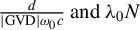 $\frac{d}{\left|\mathrm{GVD}\right|{\omega}_0c}\;\mathrm{and}\kern0.24em {\lambda}_0N$
. Below we will compare these geometries in terms of focal intensity and power, which, according to Equations (11) and (13), linearly depend on another parameter,
$\frac{d}{\left|\mathrm{GVD}\right|{\omega}_0c}\;\mathrm{and}\kern0.24em {\lambda}_0N$
. Below we will compare these geometries in terms of focal intensity and power, which, according to Equations (11) and (13), linearly depend on another parameter, $\Delta \omega R\eta {w}_\mathrm{th}$
.
$\Delta \omega R\eta {w}_\mathrm{th}$
.
5 Comparison of the geometries and discussion of the results
To begin with, we will find ${D}_\mathrm{opt}$
and optimal values of the grating sizes
${D}_\mathrm{opt}$
and optimal values of the grating sizes ${L}_\mathrm{g}$
and
${L}_\mathrm{g}$
and ${H}_\mathrm{g}$
for all four geometries. Our quantitative analysis will be restricted to two values of d: large d = 190 cm and a relatively modest d = 157 cm. The latter corresponds to the previously planned design of the SEL-100 PW facility with
${H}_\mathrm{g}$
for all four geometries. Our quantitative analysis will be restricted to two values of d: large d = 190 cm and a relatively modest d = 157 cm. The latter corresponds to the previously planned design of the SEL-100 PW facility with ${L}_\mathrm{g}=70\;\mathrm{cm}\kern0.36em \mathrm{and}\kern0.24em {H}_\mathrm{g}\,{=}\,145\;\mathrm{cm}$
[
Reference Liu, Shen, Du and Li10]. The value
${L}_\mathrm{g}=70\;\mathrm{cm}\kern0.36em \mathrm{and}\kern0.24em {H}_\mathrm{g}\,{=}\,145\;\mathrm{cm}$
[
Reference Liu, Shen, Du and Li10]. The value $d=190\;\mathrm{cm}$
is obtained from Equation (9) for the gratings currently planned for SEL-100 PW
$d=190\;\mathrm{cm}$
is obtained from Equation (9) for the gratings currently planned for SEL-100 PW $\left({L}_\mathrm{g}\ =\ 162.5\;\mathrm{cm},\ {H}_\mathrm{g}\ =\ 107\;\mathrm{cm}\ \mathrm{and}\ ;N=1320\ \mathrm{mm}^{-1}\right)$
[
Reference Liu, Wu, Liu, Wang, Xu and Leng45]. The values of
$\left({L}_\mathrm{g}\ =\ 162.5\;\mathrm{cm},\ {H}_\mathrm{g}\ =\ 107\;\mathrm{cm}\ \mathrm{and}\ ;N=1320\ \mathrm{mm}^{-1}\right)$
[
Reference Liu, Wu, Liu, Wang, Xu and Leng45]. The values of ${\lambda}_0$
and the GVD in the SEL-100 PW (
${\lambda}_0$
and the GVD in the SEL-100 PW ( ${{\lambda}_0=920\;\mathrm{nm}}$
, GVD = −4.2 ps2) and XCELS (
${{\lambda}_0=920\;\mathrm{nm}}$
, GVD = −4.2 ps2) and XCELS ( ${\lambda}_0=910\;\mathrm{nm}$
, GVD = −4.4 ps2) projects are almost the same, and the difference in
${\lambda}_0=910\;\mathrm{nm}$
, GVD = −4.4 ps2) projects are almost the same, and the difference in ${D}_\mathrm{opt}$
is negligible. The gratings are frequently written at the wavelength
${D}_\mathrm{opt}$
is negligible. The gratings are frequently written at the wavelength ${\lambda}_\mathrm{wr}=413\;\mathrm{nm}$
that we used in our calculations.
${\lambda}_\mathrm{wr}=413\;\mathrm{nm}$
that we used in our calculations.
The ${D}_\mathrm{opt}(N)$
curves for the two values of
${D}_\mathrm{opt}(N)$
curves for the two values of $d$
mentioned above are plotted in Figure 4(a) for all the considered geometries. At
$d$
mentioned above are plotted in Figure 4(a) for all the considered geometries. At $N>1405\ \mathrm{mm}^{-1}$
and
$N>1405\ \mathrm{mm}^{-1}$
and $d=190\;\mathrm{cm},$
there is no angle
$d=190\;\mathrm{cm},$
there is no angle $\gamma$
, which satisfies the decoupling condition (Equation (20)) for the F2LC. The
$\gamma$
, which satisfies the decoupling condition (Equation (20)) for the F2LC. The ${\alpha}_\mathrm{opt}-{\alpha}_\mathrm{L}$
difference for the plane geometries for the F4TC and F2TC and the angle
${\alpha}_\mathrm{opt}-{\alpha}_\mathrm{L}$
difference for the plane geometries for the F4TC and F2TC and the angle ${\gamma}_\mathrm{opt}$
for the out-of-plane F2LC and F2SC as a function of N are plotted in Figure 4(b). From Figure 4(a) it is clear that the F2SC provides maximum
${\gamma}_\mathrm{opt}$
for the out-of-plane F2LC and F2SC as a function of N are plotted in Figure 4(b). From Figure 4(a) it is clear that the F2SC provides maximum ${D}_\mathrm{opt}$
at any N and small values of N are preferable for all geometries. However, it is technologically difficult to produce gratings with small N, especially at large
${D}_\mathrm{opt}$
at any N and small values of N are preferable for all geometries. However, it is technologically difficult to produce gratings with small N, especially at large ${\alpha}_\mathrm{opt}-{\alpha}_\mathrm{L}$
, that is, for the F4TC, where at
${\alpha}_\mathrm{opt}-{\alpha}_\mathrm{L}$
, that is, for the F4TC, where at $N=1200\ \mathrm{mm}^{-1},$ ${\alpha}_\mathrm{opt}-{\alpha}_\mathrm{L}=17.2{}^{\circ}$
with
${\alpha}_\mathrm{opt}-{\alpha}_\mathrm{L}=17.2{}^{\circ}$
with $d=190\;\mathrm{cm}$
(Figure 4(b)). With such parameters it is hard to provide a high diffraction efficiency R of the grating in a wide band, so it is reasonable to consider
$d=190\;\mathrm{cm}$
(Figure 4(b)). With such parameters it is hard to provide a high diffraction efficiency R of the grating in a wide band, so it is reasonable to consider $N=1320\ \mathrm{mm}^{-1}$
and more, although in this case the angle
$N=1320\ \mathrm{mm}^{-1}$
and more, although in this case the angle ${\alpha}_\mathrm{opt}-{\alpha}_\mathrm{L}$
is even larger. For the F2LC and F2SC,
${\alpha}_\mathrm{opt}-{\alpha}_\mathrm{L}$
is even larger. For the F2LC and F2SC, ${\alpha}_\mathrm{opt}={\alpha}_\mathrm{L}$
and
${\alpha}_\mathrm{opt}={\alpha}_\mathrm{L}$
and $N=1200\ \mathrm{mm}^{-1}$
and even
$N=1200\ \mathrm{mm}^{-1}$
and even $N=1080\ \mathrm{mm}^{-1}$
may be acceptable, especially for a relatively small band. At the same time, in these out-of-plane compressors the angle
$N=1080\ \mathrm{mm}^{-1}$
may be acceptable, especially for a relatively small band. At the same time, in these out-of-plane compressors the angle ${\gamma}_\mathrm{opt}$
is nonzero, and its large values also lead to a decrease in the grating efficiency, which may be significant at
${\gamma}_\mathrm{opt}$
is nonzero, and its large values also lead to a decrease in the grating efficiency, which may be significant at $\gamma \ge 10{}^{\circ}$
[
Reference Smith, Erdogan and Erdogan36,
Reference Han, Li, Zhang, Kong, Cao, Jin, Leng, Li and Shao68]. From the point of view of reducing
$\gamma \ge 10{}^{\circ}$
[
Reference Smith, Erdogan and Erdogan36,
Reference Han, Li, Zhang, Kong, Cao, Jin, Leng, Li and Shao68]. From the point of view of reducing ${\gamma}_\mathrm{opt}$
it is also more advantageous to use small N (Figure 4(b)).
${\gamma}_\mathrm{opt}$
it is also more advantageous to use small N (Figure 4(b)).
Curves for ${D}_\mathrm{opt}$
(а) and for the
${D}_\mathrm{opt}$
(а) and for the ${\alpha}_\mathrm{opt}-{\alpha}_\mathrm{L}$
difference (F4TC, F2TC) and for
${\alpha}_\mathrm{opt}-{\alpha}_\mathrm{L}$
difference (F4TC, F2TC) and for ${\gamma}_\mathrm{opt}$
(F2LC, F2SC) (b) plotted for the F4TC (green triangles), F2ТC (blue circles), F2LC (black diamonds) and F2SC (red squares) for
${\gamma}_\mathrm{opt}$
(F2LC, F2SC) (b) plotted for the F4TC (green triangles), F2ТC (blue circles), F2LC (black diamonds) and F2SC (red squares) for $d=190\;\mathrm{cm}$
(open symbols) and
$d=190\;\mathrm{cm}$
(open symbols) and $d=157\;\mathrm{cm}$
(filled symbols).
$d=157\;\mathrm{cm}$
(filled symbols).

As the optimal angles ${\alpha}_\mathrm{opt}$
and
${\alpha}_\mathrm{opt}$
and ${\gamma}_\mathrm{opt}$
are minimal angles that ensure decoupling (see Section 3), then for a given N they simultaneously ensure maximum diffraction efficiency R (it is taken into account that
${\gamma}_\mathrm{opt}$
are minimal angles that ensure decoupling (see Section 3), then for a given N they simultaneously ensure maximum diffraction efficiency R (it is taken into account that ${\alpha}_\mathrm{opt}>{\alpha}_\mathrm{L}$
, hence minimal α corresponds to minimal
${\alpha}_\mathrm{opt}>{\alpha}_\mathrm{L}$
, hence minimal α corresponds to minimal $\alpha -{\alpha}_\mathrm{L}$
). From this it follows that, despite the assumption
$\alpha -{\alpha}_\mathrm{L}$
). From this it follows that, despite the assumption $R= const$
, the results of the analysis including the plots in Figure 4 do not depend on the type of the function
$R= const$
, the results of the analysis including the plots in Figure 4 do not depend on the type of the function $R\left(\Delta \omega, N,\alpha, \gamma \right)$
. With known
$R\left(\Delta \omega, N,\alpha, \gamma \right)$
. With known ${D}_\mathrm{opt}$
,
${D}_\mathrm{opt}$
, ${\alpha}_\mathrm{opt}$
and
${\alpha}_\mathrm{opt}$
and ${\gamma}_\mathrm{opt}$
, optimal grating dimensions can be readily found from Equations (6)–(8). In other words, regardless of the type of the function R
${\gamma}_\mathrm{opt}$
, optimal grating dimensions can be readily found from Equations (6)–(8). In other words, regardless of the type of the function R $\left(\Delta\omega, N,\alpha, \gamma \right)$
, we have found all optimal compressor parameters that allow us to achieve the maximum of all energy quantities
$\left(\Delta\omega, N,\alpha, \gamma \right)$
, we have found all optimal compressor parameters that allow us to achieve the maximum of all energy quantities $I,P,W$
for each N and each geometry.
$I,P,W$
for each N and each geometry.
For calculating the absolute values of I, P and W from Equations (11) and (13), a few more constants need to be specified. We do not have explicit data for the $R\left(\Delta\omega, N,\alpha, \gamma \right)$
function, so we set
$R\left(\Delta\omega, N,\alpha, \gamma \right)$
function, so we set $R= const=0.92$
and will interpret the obtained results taking into account the vulnerability of the variants with small N and simultaneously large
$R= const=0.92$
and will interpret the obtained results taking into account the vulnerability of the variants with small N and simultaneously large ${\alpha}_\mathrm{opt}-{\alpha}_\mathrm{L}$
or
${\alpha}_\mathrm{opt}-{\alpha}_\mathrm{L}$
or ${\gamma}_\mathrm{opt}$
mentioned above. For the threshold value of fluence on the surface normal to the wave vector of the incident beam
${\gamma}_\mathrm{opt}$
mentioned above. For the threshold value of fluence on the surface normal to the wave vector of the incident beam ${w}_{\mathrm{th}}$
, different data are available in the literature (for single-shot lasers with 13–30 fs pulses): 575 mJ/cm2 (measured at
${w}_{\mathrm{th}}$
, different data are available in the literature (for single-shot lasers with 13–30 fs pulses): 575 mJ/cm2 (measured at $\alpha =50{}^{\circ}$
)[
Reference Han, Li, Zhang, Kong, Cao, Jin, Leng, Li and Shao68]; 0.596 J/cm2 (measured at
$\alpha =50{}^{\circ}$
)[
Reference Han, Li, Zhang, Kong, Cao, Jin, Leng, Li and Shao68]; 0.596 J/cm2 (measured at $\alpha =62{}^{\circ}$
)[
Reference Han, Li, Zhang, Kong, Cao, Jin, Leng, Li and Shao68]; 400 mJ/cm2 (measured at
$\alpha =62{}^{\circ}$
)[
Reference Han, Li, Zhang, Kong, Cao, Jin, Leng, Li and Shao68]; 400 mJ/cm2 (measured at $\alpha =53{}^{\circ}$
)[
Reference Han, Jin, Kong, Wang, Zhang, Cao, Cui and Shao70]; 470 mJ/cm2 (measured at
$\alpha =53{}^{\circ}$
)[
Reference Han, Jin, Kong, Wang, Zhang, Cao, Cui and Shao70]; 470 mJ/cm2 (measured at $\alpha =61{}^{\circ}$
)[
Reference Liu, Shen, Du and Li10]; 660 mJ/cm2 (measured at
$\alpha =61{}^{\circ}$
)[
Reference Liu, Shen, Du and Li10]; 660 mJ/cm2 (measured at $\alpha =46{}^{\circ}$
)[
Reference Poole, Trendafilov, Shvets, Smith and Chowdhury71]; and 377 mJ/cm2 (at
$\alpha =46{}^{\circ}$
)[
Reference Poole, Trendafilov, Shvets, Smith and Chowdhury71]; and 377 mJ/cm2 (at $\alpha =58{}^{\circ}$
)[
Reference Liu, Wu, Liu, Wang, Xu and Leng45]. In our earlier works[
Reference Khazanov, Shaykin, Kostyukov, Ginzburg, Mukhin, Yakovlev, Soloviev, Kuznetsov, Mironov, Korzhimanov, Bulanov, Shaikin, Kochetkov, Kuzmin, Martyanov, Lozhkarev, Starodubtsev, Litvak and Sergeev5,
Reference Khazanov41] the data of Ref. [Reference Liu, Shen, Du and Li10] were used in the calculations, but now we will take the data from the most recent paper[
Reference Liu, Wu, Liu, Wang, Xu and Leng45], where the minimum of the indicated values
$\alpha =58{}^{\circ}$
)[
Reference Liu, Wu, Liu, Wang, Xu and Leng45]. In our earlier works[
Reference Khazanov, Shaykin, Kostyukov, Ginzburg, Mukhin, Yakovlev, Soloviev, Kuznetsov, Mironov, Korzhimanov, Bulanov, Shaikin, Kochetkov, Kuzmin, Martyanov, Lozhkarev, Starodubtsev, Litvak and Sergeev5,
Reference Khazanov41] the data of Ref. [Reference Liu, Shen, Du and Li10] were used in the calculations, but now we will take the data from the most recent paper[
Reference Liu, Wu, Liu, Wang, Xu and Leng45], where the minimum of the indicated values ${w}_{\mathrm{th}}=0.377$
J/cm2 was presented. This allows us to compare the obtained results with the results reported in Ref. [Reference Liu, Wu, Liu, Wang, Xu and Leng45]. Note that this value of
${w}_{\mathrm{th}}=0.377$
J/cm2 was presented. This allows us to compare the obtained results with the results reported in Ref. [Reference Liu, Wu, Liu, Wang, Xu and Leng45]. Note that this value of ${w}_{\mathrm{th}}$
is the smallest of those indicated above.
${w}_{\mathrm{th}}$
is the smallest of those indicated above.
As shown in Section 3, all energy quantities will be smaller if the damage threshold is determined by the fluence on the grating surface rather than by the beam fluence ${w}_{\mathrm{th}}$
. In this pessimistic version, we designate them as
${w}_{\mathrm{th}}$
. In this pessimistic version, we designate them as ${I}_\mathrm{p},{P}_\mathrm{p},{W}_\mathrm{p}$
. Whereas for calculations in the optimistic case we use
${I}_\mathrm{p},{P}_\mathrm{p},{W}_\mathrm{p}$
. Whereas for calculations in the optimistic case we use ${{w}_{\mathrm{th}}=377\;\mathrm{mJ}/{\mathrm{cm}}^2}$
obtained at
${{w}_{\mathrm{th}}=377\;\mathrm{mJ}/{\mathrm{cm}}^2}$
obtained at $\alpha =58{}^{\circ}$
, for obtaining
$\alpha =58{}^{\circ}$
, for obtaining ${I}_\mathrm{p},{P}_\mathrm{p},{W}_\mathrm{p}$
it is necessary to multiply
${I}_\mathrm{p},{P}_\mathrm{p},{W}_\mathrm{p}$
it is necessary to multiply $I,P,W$
by
$I,P,W$
by ${\cos}\left(58{}^{\circ}\right)/ \cos\alpha$
, where
${\cos}\left(58{}^{\circ}\right)/ \cos\alpha$
, where $\alpha ={\alpha}_\mathrm{opt}$
for plane compressors and
$\alpha ={\alpha}_\mathrm{opt}$
for plane compressors and $\alpha ={\alpha}_\mathrm{L}$
for out-of-plane compressors. When calculating
$\alpha ={\alpha}_\mathrm{L}$
for out-of-plane compressors. When calculating $I$
and
$I$
and ${I}_\mathrm{p}$
, we assume that for the focusing parabola
${I}_\mathrm{p}$
, we assume that for the focusing parabola ${F}_{\#}=2,$
which seems quite realistic.
${F}_{\#}=2,$
which seems quite realistic.
The safety factor $\eta$
is chosen such that the damage of the last grating should be excluded even in ‘unsuccessful’ shots. Since I, P, W are proportional to
$\eta$
is chosen such that the damage of the last grating should be excluded even in ‘unsuccessful’ shots. Since I, P, W are proportional to $\eta$
, its increase is very important. The reasons for the laser-induced damage at
$\eta$
, its increase is very important. The reasons for the laser-induced damage at $\eta <1$
(i.e., at
$\eta <1$
(i.e., at $w<{w}_{\mathrm{th}}$
) are the instability of the pulse energy from shot to shot and hot spots on the last grating caused by fluence fluctuations over the beam aperture. The first reason is not related to the compressor geometry, while the second one is. For the F4TC we will take
$w<{w}_{\mathrm{th}}$
) are the instability of the pulse energy from shot to shot and hot spots on the last grating caused by fluence fluctuations over the beam aperture. The first reason is not related to the compressor geometry, while the second one is. For the F4TC we will take $\eta =0.5$
, which is most often used in the literature[
Reference Liu, Shen, Du and Li10,
Reference Liu, Wu, Liu, Wang, Xu and Leng45,
Reference Shen, Du, Liang, Wang, Liu and Li48,
Reference Du, Shen, Liang, Wang, Liu and Li57]. Thus, for the F4TC, the product
$\eta =0.5$
, which is most often used in the literature[
Reference Liu, Shen, Du and Li10,
Reference Liu, Wu, Liu, Wang, Xu and Leng45,
Reference Shen, Du, Liang, Wang, Liu and Li48,
Reference Du, Shen, Liang, Wang, Liu and Li57]. Thus, for the F4TC, the product ${R\eta w}_{\mathrm{th}}$
, on which
${R\eta w}_{\mathrm{th}}$
, on which $I,P,W$
depend linearly (Equations (11) and (13)), is equal to
$I,P,W$
depend linearly (Equations (11) and (13)), is equal to $173\;\mathrm{mJ}/{\mathrm{cm}}^2$
, like in Ref. [Reference Liu, Wu, Liu, Wang, Xu and Leng45]. This will ensure correct comparison of our results with the data reported in Ref. [Reference Liu, Wu, Liu, Wang, Xu and Leng45]. Note that in Refs. [Reference Khazanov, Shaykin, Kostyukov, Ginzburg, Mukhin, Yakovlev, Soloviev, Kuznetsov, Mironov, Korzhimanov, Bulanov, Shaikin, Kochetkov, Kuzmin, Martyanov, Lozhkarev, Starodubtsev, Litvak and Sergeev5,Reference Khazanov41] the results were obtained for
$173\;\mathrm{mJ}/{\mathrm{cm}}^2$
, like in Ref. [Reference Liu, Wu, Liu, Wang, Xu and Leng45]. This will ensure correct comparison of our results with the data reported in Ref. [Reference Liu, Wu, Liu, Wang, Xu and Leng45]. Note that in Refs. [Reference Khazanov, Shaykin, Kostyukov, Ginzburg, Mukhin, Yakovlev, Soloviev, Kuznetsov, Mironov, Korzhimanov, Bulanov, Shaikin, Kochetkov, Kuzmin, Martyanov, Lozhkarev, Starodubtsev, Litvak and Sergeev5,Reference Khazanov41] the results were obtained for ${R\eta w}_{\mathrm{th}}=251\;\mathrm{mJ}/{\mathrm{cm}}^2$
, which means that for comparison with these works all the values of I, P, W obtained below should be multiplied by 1.34. As discussed above, the key advantage of two-grating compressors is the dramatic reduction of fluence fluctuations on the output grating. In fact, the fluence fluctuations on the second grating are negligibly small and the only reason for η to differ from unity is that the pulse energy jumps from shot to shot. For all three two-grating geometries we will take
${R\eta w}_{\mathrm{th}}=251\;\mathrm{mJ}/{\mathrm{cm}}^2$
, which means that for comparison with these works all the values of I, P, W obtained below should be multiplied by 1.34. As discussed above, the key advantage of two-grating compressors is the dramatic reduction of fluence fluctuations on the output grating. In fact, the fluence fluctuations on the second grating are negligibly small and the only reason for η to differ from unity is that the pulse energy jumps from shot to shot. For all three two-grating geometries we will take $\eta =0.75$
, that is, we allow a random increase in the input pulse energy by a factor of
$\eta =0.75$
, that is, we allow a random increase in the input pulse energy by a factor of $1/\eta =1.33$
, which seems to be a very conservative value. Thus, for the F2TC, F2LC and F2SC,
$1/\eta =1.33$
, which seems to be a very conservative value. Thus, for the F2TC, F2LC and F2SC, ${R\eta w}_{\mathrm{th}}$
is 0.260 J/cm2. In any case, if
${R\eta w}_{\mathrm{th}}$
is 0.260 J/cm2. In any case, if ${R\eta w}_{\mathrm{th}}$
differs from 0.260 J/cm2 (or from 0.173 J/cm2 for the F4TC) by a factor of K, then all I, P, W values that will be obtained below should be multiplied by K.
${R\eta w}_{\mathrm{th}}$
differs from 0.260 J/cm2 (or from 0.173 J/cm2 for the F4TC) by a factor of K, then all I, P, W values that will be obtained below should be multiplied by K.
The $I(N)$
and
$I(N)$
and ${I}_\mathrm{p}(N)$
functions for the above d values are shown in Figure 5 and similar
${I}_\mathrm{p}(N)$
functions for the above d values are shown in Figure 5 and similar $P(N)$
and
$P(N)$
and ${P}_\mathrm{p}(N)$
functions are shown in Figure 6 for all four compressor geometries. The spectrum width is 240 nm as in SEL-100 PW[
Reference Liu, Wu, Liu, Wang, Xu and Leng45]. In XCELS, the spectrum width is 1.58 times narrower – 150 nm[
Reference Khazanov, Shaykin, Kostyukov, Ginzburg, Mukhin, Yakovlev, Soloviev, Kuznetsov, Mironov, Korzhimanov, Bulanov, Shaikin, Kochetkov, Kuzmin, Martyanov, Lozhkarev, Starodubtsev, Litvak and Sergeev5]; the differences will be discussed below. The two most sensitive assumptions in the above theory are a flat-top spectral profile and
${P}_\mathrm{p}(N)$
functions are shown in Figure 6 for all four compressor geometries. The spectrum width is 240 nm as in SEL-100 PW[
Reference Liu, Wu, Liu, Wang, Xu and Leng45]. In XCELS, the spectrum width is 1.58 times narrower – 150 nm[
Reference Khazanov, Shaykin, Kostyukov, Ginzburg, Mukhin, Yakovlev, Soloviev, Kuznetsov, Mironov, Korzhimanov, Bulanov, Shaikin, Kochetkov, Kuzmin, Martyanov, Lozhkarev, Starodubtsev, Litvak and Sergeev5]; the differences will be discussed below. The two most sensitive assumptions in the above theory are a flat-top spectral profile and $\Delta \omega \ll {\omega}_0$
. The results of numerical simulation for the super-Gaussian spectral profile
$\Delta \omega \ll {\omega}_0$
. The results of numerical simulation for the super-Gaussian spectral profile $\mathit{\exp}\left(-{\left(\frac{\omega -{\omega}_0}{\Delta \omega}\right)}^{12}\right)$
are shown by dotted curves. The focal intensity is in a very good agreement with Equation (11), even for the huge 240 nm bandwidth. The accuracy of Equation (13) is not so high, as the simulations showed about a 10% difference in power compared to Equation (13), but this is still acceptable.
$\mathit{\exp}\left(-{\left(\frac{\omega -{\omega}_0}{\Delta \omega}\right)}^{12}\right)$
are shown by dotted curves. The focal intensity is in a very good agreement with Equation (11), even for the huge 240 nm bandwidth. The accuracy of Equation (13) is not so high, as the simulations showed about a 10% difference in power compared to Equation (13), but this is still acceptable.
The dependence of the focal intensity $I$
on
$I$
on $N$
in the optimistic (а) and pessimistic (b) variants for the F4TC (green triangles), F2ТC (blue circles), F2LC (black diamonds) and F2SC (red squares) for
$N$
in the optimistic (а) and pessimistic (b) variants for the F4TC (green triangles), F2ТC (blue circles), F2LC (black diamonds) and F2SC (red squares) for $d=190\;\mathrm{cm}$
(open symbols) and
$d=190\;\mathrm{cm}$
(open symbols) and $d=157\;\mathrm{cm}$
(filled symbols). Dotted curves show results of numerical simulation.
$d=157\;\mathrm{cm}$
(filled symbols). Dotted curves show results of numerical simulation. $\Delta \omega /{\omega}_0=0.130$
(SEL-100 PW).
$\Delta \omega /{\omega}_0=0.130$
(SEL-100 PW).

The dependence of the output power $P$
on
$P$
on $N$
in the optimistic (а) and pessimistic (b) variants for the F4TC (green triangles), F2ТC (blue circles), F2LC (black diamonds) and F2SC (red squares) for
$N$
in the optimistic (а) and pessimistic (b) variants for the F4TC (green triangles), F2ТC (blue circles), F2LC (black diamonds) and F2SC (red squares) for $d=190\;\mathrm{cm}$
(open symbols) and
$d=190\;\mathrm{cm}$
(open symbols) and $d=157\;\mathrm{cm}$
(filled symbols). Dotted curves show results of numerical simulation.
$d=157\;\mathrm{cm}$
(filled symbols). Dotted curves show results of numerical simulation. $\Delta \omega /{\omega}_0=0.130$
(SEL-100 PW).
$\Delta \omega /{\omega}_0=0.130$
(SEL-100 PW).

It is clear from the figures that in both optimistic and pessimistic cases, the F4TC and F2LC are inferior to the F2TC and F2SC, which is true for both d values. Physically, this is explained by the lack of fluctuation smoothing on the last grating in the F4TC and the fact that in the F2LC the beam footprint on the grating is a parallelogram (Figure 2, middle row), which reduces the beam size for the same grating dimensions. The difference in $P$
between the F2TC and F2SC is small in the optimistic case, and the F2TC is preferable in the pessimistic case. However, it is important to remind readers that Figures 5 and 6 are plotted for
$P$
between the F2TC and F2SC is small in the optimistic case, and the F2TC is preferable in the pessimistic case. However, it is important to remind readers that Figures 5 and 6 are plotted for $R=0.92$
for all geometries. Here, R is maximal at
$R=0.92$
for all geometries. Here, R is maximal at $\alpha ={\alpha}_\mathrm{L}$
and at
$\alpha ={\alpha}_\mathrm{L}$
and at $\gamma =0$
. Since the second condition is satisfied for the F2TC and the first for the F2SC, the allowance for the
$\gamma =0$
. Since the second condition is satisfied for the F2TC and the first for the F2SC, the allowance for the $R\left(\alpha, \gamma \right)$
function (we do not know it) may change the relationship between the F2TC and F2SC.
$R\left(\alpha, \gamma \right)$
function (we do not know it) may change the relationship between the F2TC and F2SC.
The best values of N are also slightly different in the optimistic and pessimistic variants. Small N is preferable in the optimistic case; in the pessimistic case N impacts little. This is explained by quite substantial losses that are inversely proportional to N in all two-grating compressors (see Equation (12)). As a result, ${I}_\mathrm{p}(N)$
and
${I}_\mathrm{p}(N)$
and ${P}_\mathrm{p}(N)$
do not decrease with increasing N, despite the decrease in the beam size
${P}_\mathrm{p}(N)$
do not decrease with increasing N, despite the decrease in the beam size ${D}_\mathrm{opt}$
(Figure 4(a)). It is important to remember that the angle
${D}_\mathrm{opt}$
(Figure 4(a)). It is important to remember that the angle ${\gamma}_\mathrm{opt}$
increases with increasing N (Figure 4(b)), which leads to a decrease in
${\gamma}_\mathrm{opt}$
increases with increasing N (Figure 4(b)), which leads to a decrease in $R$
. All compressor parameters are summarized in Table 2 for all geometries for the considered N values. For the F4TC and F2TC we chose
$R$
. All compressor parameters are summarized in Table 2 for all geometries for the considered N values. For the F4TC and F2TC we chose $N=1320\ \mathrm{mm}^{-1}$
, as at lower N it is difficult to create gratings with high
$N=1320\ \mathrm{mm}^{-1}$
, as at lower N it is difficult to create gratings with high $R$
at
$R$
at $\alpha >{\alpha}_\mathrm{L}$
. For the same reason,
$\alpha >{\alpha}_\mathrm{L}$
. For the same reason, $N=1200\ \mathrm{mm}^{-1}$
was chosen for the F2LC and F2LC because
$N=1200\ \mathrm{mm}^{-1}$
was chosen for the F2LC and F2LC because $N=1080\ \mathrm{mm}^{-1}$
is challenging even at
$N=1080\ \mathrm{mm}^{-1}$
is challenging even at $\alpha ={\alpha}_\mathrm{L}$
.
$\alpha ={\alpha}_\mathrm{L}$
.
Parameters of four geometries of full-aperture compressors (the values for $d=190\;\mathrm{cm}$
and
$d=190\;\mathrm{cm}$
and $d=157\;\mathrm{cm}$
are separated with the slash).
$d=157\;\mathrm{cm}$
are separated with the slash).

For $d=190\;\mathrm{cm},$
the F4TC allows one to achieve the power
$d=190\;\mathrm{cm},$
the F4TC allows one to achieve the power $P=114\;\mathrm{PW}$
and
$P=114\;\mathrm{PW}$
and ${P}_\mathrm{p}=111\;\mathrm{PW}$
, which are a little higher than in the design proposed in Ref. [Reference Liu, Wu, Liu, Wang, Xu and Leng45]. This is a consequence of the optimization presented above. As for the best geometries – the F2TC and F2SC – the results are more impressive:
${P}_\mathrm{p}=111\;\mathrm{PW}$
, which are a little higher than in the design proposed in Ref. [Reference Liu, Wu, Liu, Wang, Xu and Leng45]. This is a consequence of the optimization presented above. As for the best geometries – the F2TC and F2SC – the results are more impressive: ${P=186\;\mathrm{PW}}$
and
${P=186\;\mathrm{PW}}$
and $183\;\mathrm{PW}$
. Even in the pessimistic variant it is possible to achieve the power
$183\;\mathrm{PW}$
. Even in the pessimistic variant it is possible to achieve the power ${P}_\mathrm{p}=93\;\mathrm{PW}$
with a much smaller grating size of 133 cm × 91 cm for the F2TC and
${P}_\mathrm{p}=93\;\mathrm{PW}$
with a much smaller grating size of 133 cm × 91 cm for the F2TC and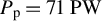 ${P}_\mathrm{p}=71\;\mathrm{PW}$
with grating size of 124 cm × 102 cm for the F2SC.
${P}_\mathrm{p}=71\;\mathrm{PW}$
with grating size of 124 cm × 102 cm for the F2SC.
As mentioned above, in the SEL-100 PW project all radiation parameters are the same as in the XCELS project except for the pulse spectrum width $\Delta \omega$
. In a conventional TC, the focal intensity I and power P are proportional to
$\Delta \omega$
. In a conventional TC, the focal intensity I and power P are proportional to $\Delta \omega$
(Equation (10)), as the pulse duration is inversely proportional to
$\Delta \omega$
(Equation (10)), as the pulse duration is inversely proportional to $\Delta \omega$
. In all full-aperture compressors, losses depend on
$\Delta \omega$
. In all full-aperture compressors, losses depend on $\Delta \omega$
, but, as follows from Equations (11) and (13), the dependence is opposite – an increase in I and P with a decrease in
$\Delta \omega$
, but, as follows from Equations (11) and (13), the dependence is opposite – an increase in I and P with a decrease in $\Delta \omega$
. As a result, I and P decrease with a decrease in
$\Delta \omega$
. As a result, I and P decrease with a decrease in $\Delta \omega$
, but not so fast as in the case of the trivial dependence
$\Delta \omega$
, but not so fast as in the case of the trivial dependence $I,P\sim \Delta \omega$
. The dependences shown in Figure 7 for
$I,P\sim \Delta \omega$
. The dependences shown in Figure 7 for $\Delta \omega /{\omega}_0=0.0824$
(XCELS) are similar to those in Figure 5 that are plotted for
$\Delta \omega /{\omega}_0=0.0824$
(XCELS) are similar to those in Figure 5 that are plotted for $\Delta \omega /{\omega}_0=0.130$
(SEL-100 PW). The comparison of these two figures, for example for the F2SC, demonstrates that due to the spectrum narrowing by 1.58 times, the focal intensity I decreased only by
$\Delta \omega /{\omega}_0=0.130$
(SEL-100 PW). The comparison of these two figures, for example for the F2SC, demonstrates that due to the spectrum narrowing by 1.58 times, the focal intensity I decreased only by $\xi \approx 1.26$
and 1.2 times for
$\xi \approx 1.26$
and 1.2 times for $d=190\;\mathrm{cm}\;\mathrm{and}\;157\;\mathrm{cm}$
. Moreover, there are some other reasons that additionally reduce
$d=190\;\mathrm{cm}\;\mathrm{and}\;157\;\mathrm{cm}$
. Moreover, there are some other reasons that additionally reduce $\xi$
. We do not have data to calculate them quantitatively, so we will simply list them. Firstly, the diffraction efficiency R for narrow-band radiation is higher than for broadband radiation. Secondly, the analysis was made for an ideally flat grating surface and for ideally parallel and equidistant grooves. In a real situation, the focal intensity will be lower and this decrease is proportional to ∆ω and depends on the rms of the surface profile
$\xi$
. We do not have data to calculate them quantitatively, so we will simply list them. Firstly, the diffraction efficiency R for narrow-band radiation is higher than for broadband radiation. Secondly, the analysis was made for an ideally flat grating surface and for ideally parallel and equidistant grooves. In a real situation, the focal intensity will be lower and this decrease is proportional to ∆ω and depends on the rms of the surface profile $\sigma$
. For
$\sigma$
. For $\sigma <\lambda /200$
this decrease is negligible[
Reference Khazanov59,
Reference Khazanov65,
Reference Kochetkov and Khazanov72], but for
$\sigma <\lambda /200$
this decrease is negligible[
Reference Khazanov59,
Reference Khazanov65,
Reference Kochetkov and Khazanov72], but for $\sigma >\lambda /40$
it can be tens of percent, and in this case
$\sigma >\lambda /40$
it can be tens of percent, and in this case $\xi$
will decrease. Physically, this is explained by the deterioration of spatial focusing with increasing
$\xi$
will decrease. Physically, this is explained by the deterioration of spatial focusing with increasing $\Delta \omega$
due to space–time coupling. Thirdly, similar reasoning is valid for ‘focusing in time’. The corresponding analysis was made under the assumption that the pulse at the compressor output is Fourier-transform-limited. This is achieved by matching the dispersions of the stretcher and compressor, as well as by using an acousto-optic programmable dispersive filter[
Reference Tournois73]. However, the accuracy of this matching is nonzero, and in practice the phase of the output pulse is not flat, which lengthens the pulse and reduces I. This decrease is the greater, with the larger
$\Delta \omega$
due to space–time coupling. Thirdly, similar reasoning is valid for ‘focusing in time’. The corresponding analysis was made under the assumption that the pulse at the compressor output is Fourier-transform-limited. This is achieved by matching the dispersions of the stretcher and compressor, as well as by using an acousto-optic programmable dispersive filter[
Reference Tournois73]. However, the accuracy of this matching is nonzero, and in practice the phase of the output pulse is not flat, which lengthens the pulse and reduces I. This decrease is the greater, with the larger $\Delta \omega$
, which reduces
$\Delta \omega$
, which reduces $\xi$
. Fourthly, the above analytical results were obtained under the condition
$\xi$
. Fourthly, the above analytical results were obtained under the condition $\Delta \omega \ll {\omega}_0$
. In the exact solution, the intensity will be slightly lower and this decrease will also be proportional to
$\Delta \omega \ll {\omega}_0$
. In the exact solution, the intensity will be slightly lower and this decrease will also be proportional to $\Delta \omega$
. Thus, the increase in the band from
$\Delta \omega$
. Thus, the increase in the band from $\Delta \omega /{\omega}_0=$
0.0824 (XCELS) to
$\Delta \omega /{\omega}_0=$
0.0824 (XCELS) to $\Delta \omega /{\omega}_0=$
0.130 (SEL-100 PW), which significantly complicates the design of the entire laser, leads to an increase in the focal intensity, but only by less than 1.26 times. For
$\Delta \omega /{\omega}_0=$
0.130 (SEL-100 PW), which significantly complicates the design of the entire laser, leads to an increase in the focal intensity, but only by less than 1.26 times. For $\Delta \omega /{\omega}_0=$
0.0824 in the F2SC, it is possible to obtain the power
$\Delta \omega /{\omega}_0=$
0.0824 in the F2SC, it is possible to obtain the power $P=147\;\mathrm{PW}$
and
$P=147\;\mathrm{PW}$
and ${P}_\mathrm{p}=95\;\mathrm{PW}$
at
${P}_\mathrm{p}=95\;\mathrm{PW}$
at $d=190\;\mathrm{cm}$
(
$d=190\;\mathrm{cm}$
(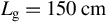 ${L}_\mathrm{g}=150\;\mathrm{cm}$
,
${L}_\mathrm{g}=150\;\mathrm{cm}$
, ${H}_\mathrm{g}=122\;\mathrm{cm}, N=1200\ \mathrm{mm}^{-1}$
), and also
${H}_\mathrm{g}=122\;\mathrm{cm}, N=1200\ \mathrm{mm}^{-1}$
), and also $P=94\;\mathrm{PW}$
and
$P=94\;\mathrm{PW}$
and ${P}_\mathrm{p}=61\;\mathrm{PW}$
at
${P}_\mathrm{p}=61\;\mathrm{PW}$
at $d=157\;\mathrm{cm}\;\left({L}_\mathrm{g}=123\;\mathrm{cm},\ {H}_\mathrm{g}=102\;\mathrm{cm},\ N=1200\ \mathrm{mm}^{-1}\right)$
. We emphasize once again that in this work we used conservative values for both
$d=157\;\mathrm{cm}\;\left({L}_\mathrm{g}=123\;\mathrm{cm},\ {H}_\mathrm{g}=102\;\mathrm{cm},\ N=1200\ \mathrm{mm}^{-1}\right)$
. We emphasize once again that in this work we used conservative values for both ${w}_{\mathrm{th}}$
and
${w}_{\mathrm{th}}$
and $\eta$
.
$\eta$
.
The dependence of the focal intensity $I$
on
$I$
on $N$
in the optimistic (а) and pessimistic (b) variants for the F4TC (green triangles), F2ТC (blue circles), F2LC (black diamonds) and F2SC (red squares) for
$N$
in the optimistic (а) and pessimistic (b) variants for the F4TC (green triangles), F2ТC (blue circles), F2LC (black diamonds) and F2SC (red squares) for $d=190\;\mathrm{cm}$
(open symbols) and
$d=190\;\mathrm{cm}$
(open symbols) and $d=157\;\mathrm{cm}$
(filled symbols). Dotted curves show results of numerical simulation.
$d=157\;\mathrm{cm}$
(filled symbols). Dotted curves show results of numerical simulation. $\Delta \omega /{\omega}_0=0.0824$
(XCELS).
$\Delta \omega /{\omega}_0=0.0824$
(XCELS).

Finally, still another important advantage of the F2SC is associated with the use of multilayer dielectric (MLD) gratings instead of gold gratings. MLD gratings have many advantages, but their main disadvantage is a sharp decrease in the diffraction efficiency with a small deviation of $\alpha$
from
$\alpha$
from ${\alpha}_\mathrm{L}$
. For example, in Ref. [Reference Alessi, Nguyen, Britten, Rosso and Haefner63] it was shown that for
${\alpha}_\mathrm{L}$
. For example, in Ref. [Reference Alessi, Nguyen, Britten, Rosso and Haefner63] it was shown that for ${{\alpha}_\mathrm{opt}-{\alpha}_\mathrm{L}=4{}^{\circ}}$
the diffraction efficiency drops from 99% to 86%. The F2TC and especially the F4TC require significantly higher values of
${{\alpha}_\mathrm{opt}-{\alpha}_\mathrm{L}=4{}^{\circ}}$
the diffraction efficiency drops from 99% to 86%. The F2TC and especially the F4TC require significantly higher values of ${\alpha}_\mathrm{opt}-{\alpha}_\mathrm{L}$
(Figure 4(b)), which makes MLD gratings unfit for them. However, if
${\alpha}_\mathrm{opt}-{\alpha}_\mathrm{L}$
(Figure 4(b)), which makes MLD gratings unfit for them. However, if $\alpha ={\alpha}_\mathrm{L}$
, at
$\alpha ={\alpha}_\mathrm{L}$
, at $\gamma =8{}^{\circ}$
(which is comparable with the requirements of the F2SC, see Figure 4(b)) the diffraction efficiency exceeds 95%[
Reference Alessi, Nguyen, Britten, Rosso and Haefner63], despite its decrease with increasing
$\gamma =8{}^{\circ}$
(which is comparable with the requirements of the F2SC, see Figure 4(b)) the diffraction efficiency exceeds 95%[
Reference Alessi, Nguyen, Britten, Rosso and Haefner63], despite its decrease with increasing $\gamma$
, as the decrease is slow. This makes it possible to use MLD gratings in the F2SC. Another shortcoming of MLD gratings is that their bandwidth is significantly narrower than that of gold gratings, so their efficiency decreases with increasing
$\gamma$
, as the decrease is slow. This makes it possible to use MLD gratings in the F2SC. Another shortcoming of MLD gratings is that their bandwidth is significantly narrower than that of gold gratings, so their efficiency decreases with increasing $\Delta \omega$
. The decrease in the compressed pulse duration and the decrease in the efficiency of a four-grating compressor as a function of
$\Delta \omega$
. The decrease in the compressed pulse duration and the decrease in the efficiency of a four-grating compressor as a function of $\Delta \omega$
for the central wavelength
$\Delta \omega$
for the central wavelength ${\lambda}_0=800\;\mathrm{nm}$
and
${\lambda}_0=800\;\mathrm{nm}$
and $N=1443\ \mathrm{mm}^{-1}$
was assessed in Ref. [Reference Alessi, Nguyen, Britten, Rosso and Haefner63]. It was shown that for a pulse duration of 17 fs, as in XCELS,
$N=1443\ \mathrm{mm}^{-1}$
was assessed in Ref. [Reference Alessi, Nguyen, Britten, Rosso and Haefner63]. It was shown that for a pulse duration of 17 fs, as in XCELS, $R=0.95$
, which is even greater than R for gold gratings. Unfortunately, the value of
$R=0.95$
, which is even greater than R for gold gratings. Unfortunately, the value of $\gamma$
is not specified in Ref. [Reference Alessi, Nguyen, Britten, Rosso and Haefner63], and separate calculations are required for
$\gamma$
is not specified in Ref. [Reference Alessi, Nguyen, Britten, Rosso and Haefner63], and separate calculations are required for ${{\lambda}_0=910\;\mathrm{nm}}$
. However, in any case, the F2SC allows using not only gold but also MLD gratings, which have a significantly higher damage threshold at the pulse duration
${{\lambda}_0=910\;\mathrm{nm}}$
. However, in any case, the F2SC allows using not only gold but also MLD gratings, which have a significantly higher damage threshold at the pulse duration $\tau =0.5-1\;\mathrm{ps}$
:
$\tau =0.5-1\;\mathrm{ps}$
: ${w}_\mathrm{th}=7\;\mathrm{J}/{\mathrm{cm}}^2$
(at
${w}_\mathrm{th}=7\;\mathrm{J}/{\mathrm{cm}}^2$
(at ${\alpha =77.2{}^{\circ}}$
)[
Reference Palmier, Neauport, Baclet, Lavastre and Dupuy74],
${\alpha =77.2{}^{\circ}}$
)[
Reference Palmier, Neauport, Baclet, Lavastre and Dupuy74], ${w}_\mathrm{th}=2\;\mathrm{J}/{\mathrm{cm}}^2$
(at
${w}_\mathrm{th}=2\;\mathrm{J}/{\mathrm{cm}}^2$
(at $\alpha =70{}^{\circ}$
)[
Reference Kong, Jin, Huang, Hong, Liu and He75],
$\alpha =70{}^{\circ}$
)[
Reference Kong, Jin, Huang, Hong, Liu and He75], ${{w}_\mathrm{th}=2.8\;\mathrm{J}/{\mathrm{cm}}^2}$
(at
${{w}_\mathrm{th}=2.8\;\mathrm{J}/{\mathrm{cm}}^2}$
(at $\alpha =76.5{}^{\circ}$
)[
Reference Alessi, Carr, Hackel, Negres, Stanion, Fair, Cross, Nissen, Luthi, Guss, Britten, Gourdin and Haefner76]. Unlike gold gratings, for which
$\alpha =76.5{}^{\circ}$
)[
Reference Alessi, Carr, Hackel, Negres, Stanion, Fair, Cross, Nissen, Luthi, Guss, Britten, Gourdin and Haefner76]. Unlike gold gratings, for which ${w}_\mathrm{th}$
does not depend on
${w}_\mathrm{th}$
does not depend on $\tau$
in the range from 100 fs to 100 ps[
Reference Stuart, Feit, Herman, Rubenchik, Shore and Perry11], for MLD gratings
$\tau$
in the range from 100 fs to 100 ps[
Reference Stuart, Feit, Herman, Rubenchik, Shore and Perry11], for MLD gratings ${w}_\mathrm{th}$
is proportional to
${w}_\mathrm{th}$
is proportional to ${\tau}^{0.22}$
(
${\tau}^{0.22}$
( $\tau =1,\dots, 30\;\mathrm{ps}$
)[
Reference Alessi, Carr, Hackel, Negres, Stanion, Fair, Cross, Nissen, Luthi, Guss, Britten, Gourdin and Haefner76],
$\tau =1,\dots, 30\;\mathrm{ps}$
)[
Reference Alessi, Carr, Hackel, Negres, Stanion, Fair, Cross, Nissen, Luthi, Guss, Britten, Gourdin and Haefner76], ${\tau}^{0.26}$
(
${\tau}^{0.26}$
( $\tau =0.5,\dots, 10\;\mathrm{ps}$
)[
Reference Kong, Jin, Huang, Hong, Liu and He75]. The approximation of this dependence to 10–20 fs gives values of
$\tau =0.5,\dots, 10\;\mathrm{ps}$
)[
Reference Kong, Jin, Huang, Hong, Liu and He75]. The approximation of this dependence to 10–20 fs gives values of ${w}_\mathrm{th}$
significantly higher than
${w}_\mathrm{th}$
significantly higher than ${w}_{\mathrm{th}}=377\;\mathrm{mJ}/{\mathrm{cm}}^2$
(at
${w}_{\mathrm{th}}=377\;\mathrm{mJ}/{\mathrm{cm}}^2$
(at ${\alpha =58{}^{\circ}}$
)[
Reference Liu, Wu, Liu, Wang, Xu and Leng45], which we used for gold gratings. Note, however, that the value
${\alpha =58{}^{\circ}}$
)[
Reference Liu, Wu, Liu, Wang, Xu and Leng45], which we used for gold gratings. Note, however, that the value ${w}_{\mathrm{th}}=290\;\mathrm{mJ}/{\mathrm{cm}}^2$
(at
${w}_{\mathrm{th}}=290\;\mathrm{mJ}/{\mathrm{cm}}^2$
(at $\alpha =37{}^{\circ}$
) for MLD gratings at
$\alpha =37{}^{\circ}$
) for MLD gratings at $\tau =80\;\mathrm{fs}$
given in Ref. [Reference Alessi, Nguyen, Britten, Rosso and Haefner63] is approximately equal to
$\tau =80\;\mathrm{fs}$
given in Ref. [Reference Alessi, Nguyen, Britten, Rosso and Haefner63] is approximately equal to ${w}_{\mathrm{th}}=377\mathrm{mJ}/{\mathrm{cm}}^2$
(at
${w}_{\mathrm{th}}=377\mathrm{mJ}/{\mathrm{cm}}^2$
(at $\alpha =58{}^{\circ}$
). Thus, the prospects for using MLD gratings in the F2SC require further research.
$\alpha =58{}^{\circ}$
). Thus, the prospects for using MLD gratings in the F2SC require further research.
6 Conclusion
In sub-exawatt lasers, laser-induced damage of compressor gratings is the main factor limiting the output pulse power P and energy W, as well as the focal intensity I. To lift this restriction, it seems promising to use two ideas simultaneously: (i) the full-aperture compressor in which the beam size on the first grating is the same as the grating size, and (ii) the two-grating compressor consisting of one pair of parallel gratings. The F2TC (Figure 1(b)) and F2LC (Figure 1(c)) were studied earlier. We have proposed a new geometry of the two-grating compressor – an F2SC (Figure 1(d)) with slanted-groove gratings. For comparison, we have used the F4TC (Figure 1(a)) that is most widely discussed in the literature. For all these four geometries, expressions for the optimal incidence angles and beam size ${D}_\mathrm{opt}$
at which I, P and W reach their maximum, have been obtained analytically. We have taken into account that the length of the holographic grating
${D}_\mathrm{opt}$
at which I, P and W reach their maximum, have been obtained analytically. We have taken into account that the length of the holographic grating ${L}_\mathrm{g}$
and its height
${L}_\mathrm{g}$
and its height ${H}_\mathrm{g}$
are not independent quantities, since the entire grating aperture must be completely illuminated during writing (Figure 3(a)). In other words, the grating diagonal d is given, and shortening of the grating allows one to increase its height and vice versa. The F2SC provides maximum
${H}_\mathrm{g}$
are not independent quantities, since the entire grating aperture must be completely illuminated during writing (Figure 3(a)). In other words, the grating diagonal d is given, and shortening of the grating allows one to increase its height and vice versa. The F2SC provides maximum ${D}_\mathrm{opt}$
(Figure 4(a)) at any groove density N, and it is preferable to use small values of N. It should be taken into account that the creation of gratings with small N is a complex technological task, especially for large deviations of the angle of incidence on the first grating
${D}_\mathrm{opt}$
(Figure 4(a)) at any groove density N, and it is preferable to use small values of N. It should be taken into account that the creation of gratings with small N is a complex technological task, especially for large deviations of the angle of incidence on the first grating ${\alpha}_\mathrm{opt}$
from the Littrow angle
${\alpha}_\mathrm{opt}$
from the Littrow angle ${\alpha}_\mathrm{L}$
, which is especially important for the F4TC, for which
${\alpha}_\mathrm{L}$
, which is especially important for the F4TC, for which ${\alpha}_\mathrm{opt}-{\alpha}_\mathrm{L}\approx 20{}^{\circ}$
, and least important for the F2LC and F2SC, for which
${\alpha}_\mathrm{opt}-{\alpha}_\mathrm{L}\approx 20{}^{\circ}$
, and least important for the F2LC and F2SC, for which ${\alpha}_\mathrm{opt}={\alpha}_\mathrm{L}$
.
${\alpha}_\mathrm{opt}={\alpha}_\mathrm{L}$
.
The main advantage of all two-grating compressors is the absence of hot spots on the second (last) grating due to the zeroing of fluence fluctuations ensured by spectral beam smoothing. So, the reserve is needed only for beam energy fluctuations from shot to shot, whereas for the F4TC it is necessary to take into account hot spots as well. As a result, in the F2TC, F2LC and F2SC it is possible to obtain significantly higher I, P and W values than in the F4TC without fear of laser-induced damage. The spectral beam smoothing inevitably leads to intensity front tilt in focus. As a result, the radiation does not reach the focal plane simultaneously. In other words, part of the radiation illuminates the target in advance (say, to the left of the focal point) and another part lags behind (to the right of the focal point). It negligibly impacts on the interaction with the target, because the intensity on the axis is the same[ Reference Khazanov47]. Even though the overtaking radiation illuminates the target in advance, the generated plasma does not impact on the radiation at the focal point, otherwise the plasma should move with velocity close to the speed of light[ Reference Khazanov64, Reference Khazanov77]. There is one more important advantage of all two-grating compressors. If two adaptive mirrors are placed one before and the other after the compressor, then the focal intensity will not decrease when using gratings with a non-flat surface, as well as with non-parallel and non-equidistant grooves. For the F2TC and F2LC this was rigorously proven in Ref. [Reference Khazanov59] and a completely analogous consideration showed that this is also true for the F2SC.
The analysis showed that the F2TC and F2SC are the most attractive geometries; the difference between them is small and depends on the specific parameter values, as well as on the variant of the dependence of the laser-induced damage threshold ${w}_\mathrm{th}$
on the incidence angle. In the SEL-100 PW project (
${w}_\mathrm{th}$
on the incidence angle. In the SEL-100 PW project ( $\Delta \omega /{\omega}_0=$
0.130) in the optimistic variant (
$\Delta \omega /{\omega}_0=$
0.130) in the optimistic variant ( ${w}_\mathrm{th}$
does not depend on the incidence angle α, Figures 5(a), 6(a) and 7(a)),
${w}_\mathrm{th}$
does not depend on the incidence angle α, Figures 5(a), 6(a) and 7(a)), $P=186\;\mathrm{PW}$
, and in the pessimistic one (
$P=186\;\mathrm{PW}$
, and in the pessimistic one ( ${w}_\mathrm{th}$
depends on α, Figures 5(b), 6(b) and 7(b))
${w}_\mathrm{th}$
depends on α, Figures 5(b), 6(b) and 7(b)) ${P}_\mathrm{p}=148\;\mathrm{PW}$
for the grating diagonal
${P}_\mathrm{p}=148\;\mathrm{PW}$
for the grating diagonal $d=190\;\mathrm{cm}$
with focal intensity at the F/2 parabola of 5.42 × 1024 W/cm2 and 5.46 × 1024 W/cm2.
$d=190\;\mathrm{cm}$
with focal intensity at the F/2 parabola of 5.42 × 1024 W/cm2 and 5.46 × 1024 W/cm2.
The above analysis is made assuming that the diffraction efficiency $R$
does not depend on the beam polarization. This approach is valid for plane compressors, where the beam keeps p-polarization (parallel to the plane of incidence) from input to output and the problem is scalar. For out-of-plane compressors the problem is intrinsically vectorial. Even if the input beam is p-polarized, after reflection by the first grating it becomes elliptically polarized[
Reference Smith, Erdogan and Erdogan36], and hence reflection by the second grating cannot be considered as a scalar problem. In a general case, both reflections are vectorial. This leads to two consequences impacting on focal intensity: decrease of the diffraction efficiency
$R$
does not depend on the beam polarization. This approach is valid for plane compressors, where the beam keeps p-polarization (parallel to the plane of incidence) from input to output and the problem is scalar. For out-of-plane compressors the problem is intrinsically vectorial. Even if the input beam is p-polarized, after reflection by the first grating it becomes elliptically polarized[
Reference Smith, Erdogan and Erdogan36], and hence reflection by the second grating cannot be considered as a scalar problem. In a general case, both reflections are vectorial. This leads to two consequences impacting on focal intensity: decrease of the diffraction efficiency $R$
and polarization deterioration. To accurately calculate these two impacts, one should know both the amplitude and phase of the diffracted wave for s- and p-input polarizations as a function of the wavelength. We do not know any analytical solutions of this task even for a simplest sinusoidal shape of the grooves. Moreover, in real gold gratings the groove shape is far from sinusoidal[
Reference Han, Li, Zhang, Kong, Cao, Jin, Leng, Li and Shao68] and it is usually optimized to a specific compressor geometry (
$R$
and polarization deterioration. To accurately calculate these two impacts, one should know both the amplitude and phase of the diffracted wave for s- and p-input polarizations as a function of the wavelength. We do not know any analytical solutions of this task even for a simplest sinusoidal shape of the grooves. Moreover, in real gold gratings the groove shape is far from sinusoidal[
Reference Han, Li, Zhang, Kong, Cao, Jin, Leng, Li and Shao68] and it is usually optimized to a specific compressor geometry ( $\alpha, \gamma, \Delta \omega$
, polarization). The detailed numerical study of groove shape optimization for out-of-plane compressors is a special task we are studying, and the results will be published in a separate paper. Nevertheless, the used assumption
$\alpha, \gamma, \Delta \omega$
, polarization). The detailed numerical study of groove shape optimization for out-of-plane compressors is a special task we are studying, and the results will be published in a separate paper. Nevertheless, the used assumption $\left(R= const\right)$
gives a good approach for two following reasons. Firstly, the theoretical[
Reference Smith, Erdogan and Erdogan36,
Reference Han, Li, Zhang, Kong, Cao, Jin, Leng, Li and Shao68] and experimental[
Reference Smith, Erdogan and Erdogan36,
Reference Hooker, Collier, Chekhlov, Clarke, Divall, Ertel, Foster, Hancock, Hawkes, Holligan, Langley, Lester, Neely, Parry and Wyborn40] studies showed that the diffraction efficiency
$\left(R= const\right)$
gives a good approach for two following reasons. Firstly, the theoretical[
Reference Smith, Erdogan and Erdogan36,
Reference Han, Li, Zhang, Kong, Cao, Jin, Leng, Li and Shao68] and experimental[
Reference Smith, Erdogan and Erdogan36,
Reference Hooker, Collier, Chekhlov, Clarke, Divall, Ertel, Foster, Hancock, Hawkes, Holligan, Langley, Lester, Neely, Parry and Wyborn40] studies showed that the diffraction efficiency $R$
only slightly drops if
$R$
only slightly drops if $\gamma <10{}^{\circ}-15{}^{\circ}$
. In Ref. [Reference Smith, Erdogan and Erdogan36] at
$\gamma <10{}^{\circ}-15{}^{\circ}$
. In Ref. [Reference Smith, Erdogan and Erdogan36] at $\gamma =15{}^{\circ}$
the four-grating LC throughput
$\gamma =15{}^{\circ}$
the four-grating LC throughput ${R}^4$
dropped by about 2% only compared to
${R}^4$
dropped by about 2% only compared to $\gamma =0{}^{\circ}$
. It is negligible taking into account that, for ultra-high-power lasers, the focal intensity is proportional to the first power of
$\gamma =0{}^{\circ}$
. It is negligible taking into account that, for ultra-high-power lasers, the focal intensity is proportional to the first power of $R$
; see Equation (10). Secondly, the ellipticity of the polarization itself does not reduce the focal intensity, which is reduced only if the ellipticity is frequency-dependent (spectral depolarization takes place). Hence, the impact of this negative phenomenon is proportional to
$R$
; see Equation (10). Secondly, the ellipticity of the polarization itself does not reduce the focal intensity, which is reduced only if the ellipticity is frequency-dependent (spectral depolarization takes place). Hence, the impact of this negative phenomenon is proportional to ${\left(\Delta \omega /{\omega}_0\right)}^2$
or even to
${\left(\Delta \omega /{\omega}_0\right)}^2$
or even to ${\left(\Delta \omega /{\omega}_0\right)}^4$
and is expected to be negligible.
${\left(\Delta \omega /{\omega}_0\right)}^4$
and is expected to be negligible.
In the XCELS project, the bandwidth is 1.58 times more narrow. However, due to the reduction of clipping losses, the focal intensity I is slightly lower than in the SEL-100 PW: only by a factor of 1.26 or even less than that. A more accurate value requires further research. Since the design of the entire laser for a narrow bandwidth is much simpler, from a practical point of view the bandwidth $\Delta \omega /{\omega}_0=$
0.0824 seems to be a very attractive choice. The F2SC allows one to generate a power of about 95 PW at
$\Delta \omega /{\omega}_0=$
0.0824 seems to be a very attractive choice. The F2SC allows one to generate a power of about 95 PW at $d=190\;\mathrm{cm}$
(
$d=190\;\mathrm{cm}$
( ${L}_\mathrm{g}=150\;\mathrm{cm}$
,
${L}_\mathrm{g}=150\;\mathrm{cm}$
, ${H}_\mathrm{g}=122\;\mathrm{cm})$
in the pessimistic case and 94 PW at
${H}_\mathrm{g}=122\;\mathrm{cm})$
in the pessimistic case and 94 PW at $d=157\;\mathrm{cm}\;\left({L}_\mathrm{g}=123\;\mathrm{cm},{H}_\mathrm{g}=102\;\mathrm{cm}\right)$
in the optimistic case.
$d=157\;\mathrm{cm}\;\left({L}_\mathrm{g}=123\;\mathrm{cm},{H}_\mathrm{g}=102\;\mathrm{cm}\right)$
in the optimistic case.
Compared to the F2TC, the advantage of the F2SC is usage of the gratings at the Littrow angle, which has three benefits: (i) an increase in the grating efficiency; (ii) an increase in the grating bandwidth; and (iii) a possibility of replacing gold gratings with MLD gratings, which cannot be used in TCs of high-power fs lasers because of their low efficiency even with a small deviation of $\alpha$
from
$\alpha$
from ${\alpha}_\mathrm{L}$
and in view of the relatively narrow band. Since in the F2SC
${\alpha}_\mathrm{L}$
and in view of the relatively narrow band. Since in the F2SC $\alpha ={\alpha}_\mathrm{L}$
, the first reason is irrelevant, and a narrow band may be quite sufficient for
$\alpha ={\alpha}_\mathrm{L}$
, the first reason is irrelevant, and a narrow band may be quite sufficient for $\Delta \omega /{\omega}_0=$
0.0824. The advantage of MLD gratings is a significantly higher laser damage threshold, which can more than fully compensate for the narrow band. The prospects of using MLD gratings in the F2SC require further research.
$\Delta \omega /{\omega}_0=$
0.0824. The advantage of MLD gratings is a significantly higher laser damage threshold, which can more than fully compensate for the narrow band. The prospects of using MLD gratings in the F2SC require further research.
Acknowledgments
This work was supported by the Ministry of Science and Higher Education of the Russian Federation (Project No. FFUF-2025-0011).
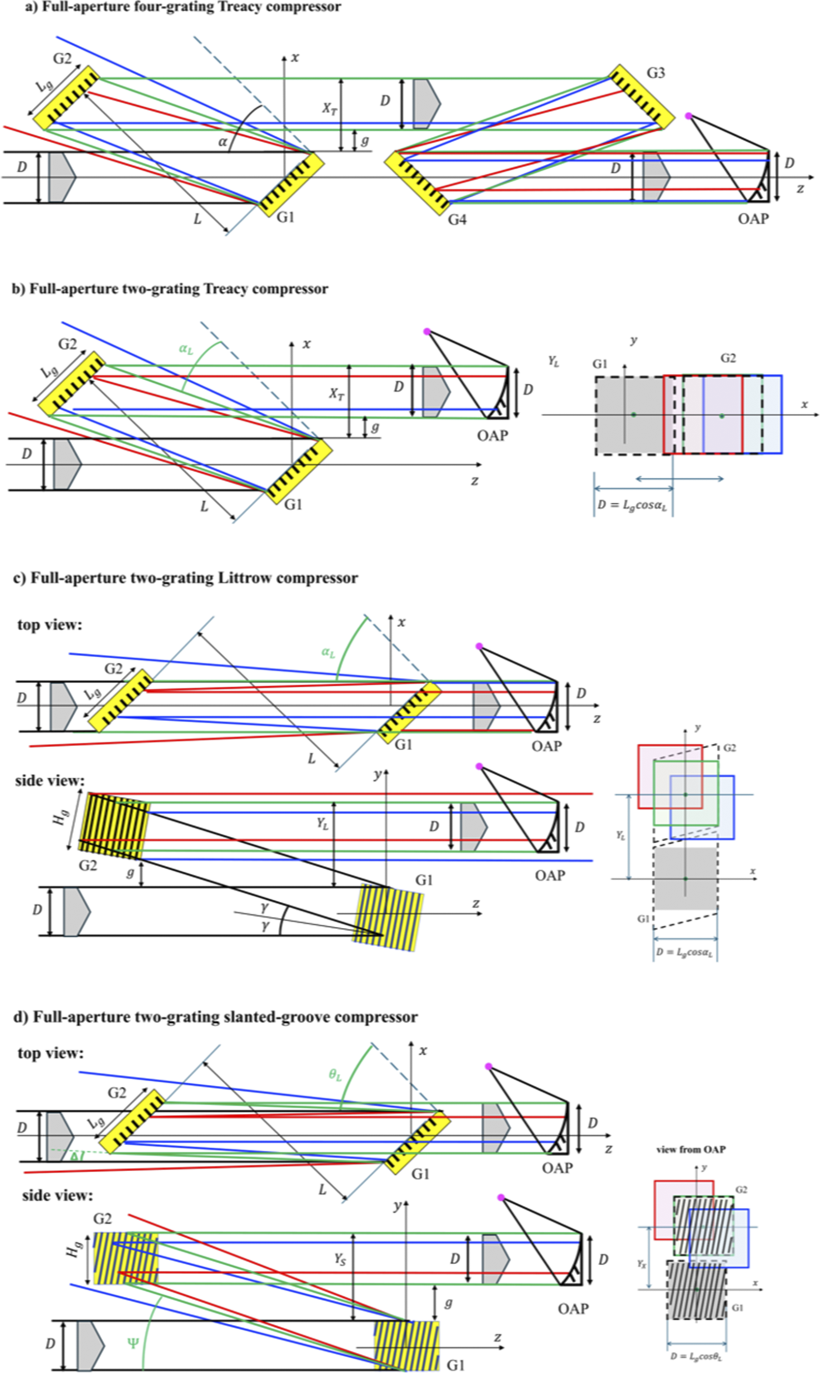
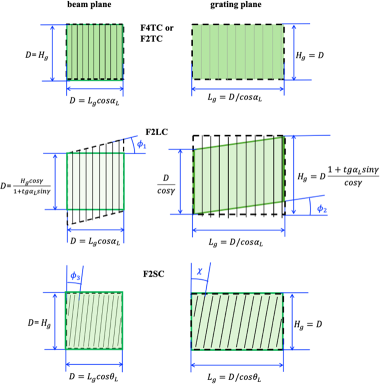
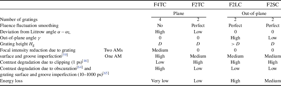
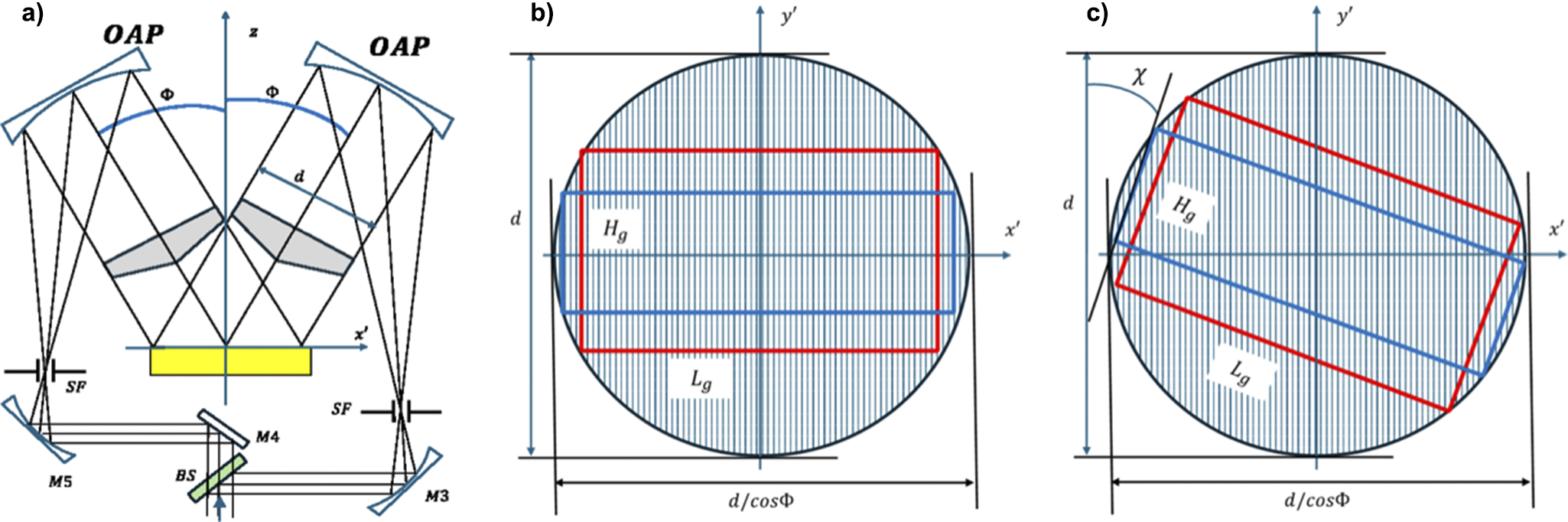


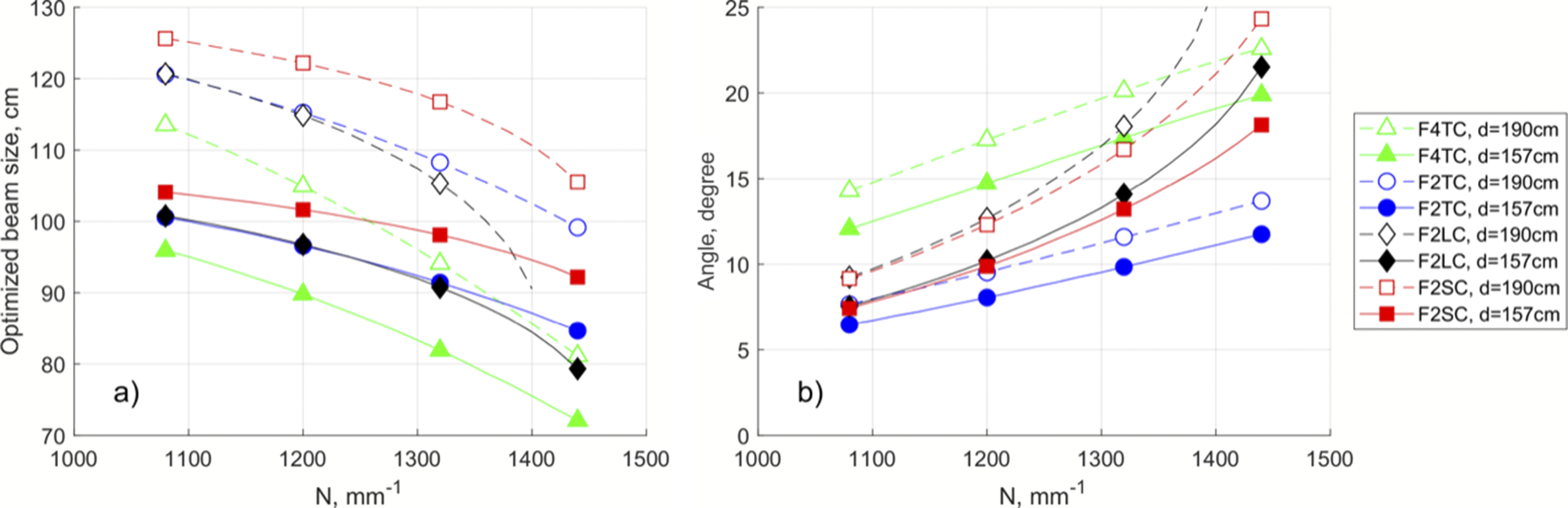


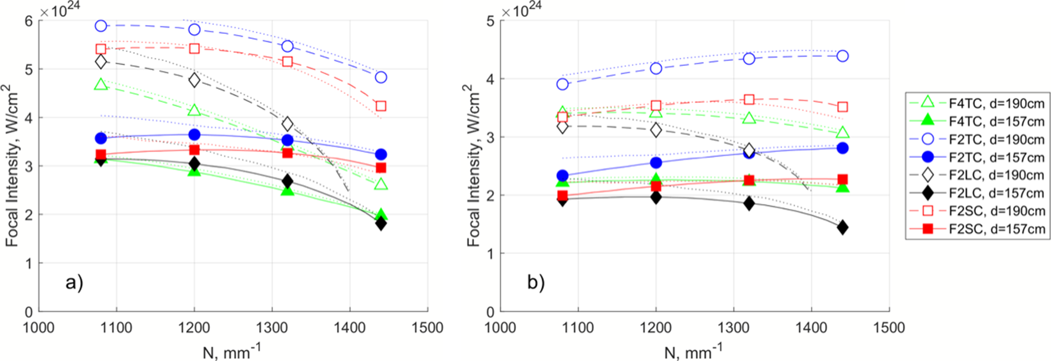


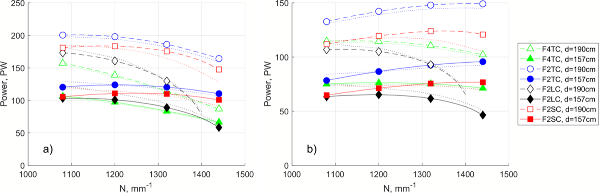


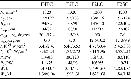


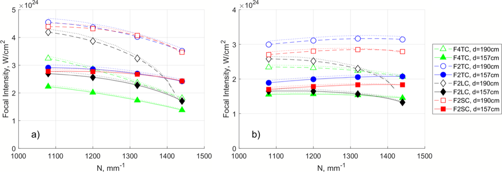


 Open access

