A) Virtual image

Let the aperture assembly be a rectangular region on a plane with (x, y) ∈ ℜReference Candès, Romberg and Tao ² coordinate system. For each point (x, y) on the aperture assembly, there is a ray starting from a point on the scene, passing through the point (x, y), and ending at the sensor, as shown in Fig. 3. Therefore, there is a unique ray associated with each point (x, y) on the aperture assembly, and its intensity arriving at the aperture assembly at time t is denoted by r(x, y;t). Then an image I(x, y) of the scene is defined as the integration of the ray in a time interval Δ t:

Fig. 3.

A ray is defined for each point on the region of aperture assembly.

(1) $$I\lpar x\comma \; y\rpar = \vint_0^{\Delta t} r\lpar x\comma \; y\semicolon \; t\rpar dt.$$

Note that the image in (1) is defined mathematically, and although it is defined in the region of the aperture assembly, there is not an actual image physically formed in the lensless compressive imaging architecture. For this reason, the image of (1) is said to be a virtual image. A virtual image I(x, y) can be considered as an analog image because it is continuously defined in the region of the aperture assembly.

Let the transmittance of the aperture assembly be defined as T(x, y). A measurement made by the sensor is the integration of the rays through the aperture assembly modulated by the transmittance, and it is given by

(2) $$\bar{z}_T = \vint \!\! \vint T\lpar x\comma \; y\rpar I \lpar x\comma \; y\rpar dxdy.$$

Although the virtual image discussed above is defined on the plane of the aperture assembly, it is not necessary to do so. The virtual image may be defined on any plane that is placed in between the sensor and the aperture assembly and parallel to the aperture assembly.

B) Digitized image

The virtual image defined by (1) can be digitized by the aperture assembly. For any given region R on the plane of the aperture assembly, we define its characteristic function as

(3) $${\bf 1}_R \lpar x\comma \; y\rpar = \left\{\matrix{ 1\comma \; \hfill &\lpar x\comma \; y\rpar \in R \cr 0 \hfill &\lpar x\comma \; y\rpar \notin R}\right..$$

Let the aperture elements of the aperture assembly be indexed by $\lpar i\comma \; j\rpar \in \open{Z}^{2}$ . We denote by E _ij the region on the plane of the aperture assembly defined by the (i, j)th aperture element as shown in Fig. 3. Each element E _ij can be used to define a pixel in the digitized image and the pixel value of the image at pixel (i, j) is the integration of the rays passing through the region E _ij and it is given by

(4) $$\eqalign{I\lpar i\comma \; j\rpar &= \vint \!\! \vint_{E_{ij}} I\lpar x\comma \; y\rpar dxdy\comma \; \cr &= \vint \!\! \vint {\bf 1}_{E_{ij}} \lpar x\comma \; y\rpar I \lpar x\comma \; y\rpar dxdy.}$$

Note that we use I(i, j) to denote a digitized image of a virtual image I(x, y) which is considered to be analog.

Equation (4) defines the digitized image I(i, j). In compressive sensing, it is often mathematically convenient to reorder a pixelized image which is a two-dimensional (2D) array into a one dimensional (1D) vector. Let q be a mapping from a 2D array to a 1D vector defined by, for example,

(5) $$\eqalign{q\colon \open{Z}^2 & \to \open{Z}\comma \; \quad \hbox{so that}\cr q\lpar i\comma \; j\rpar = i & + \lpar j - 1\rpar N_r\comma \; i\comma \; j = 1\comma \; 2\comma \; \ldots\comma \; }$$

where N _r is the number of rows in the aperture assembly. Then the pixelized image I(i, j) can be represented as a vector whose components are I _n where n = q(i, j). When there is no risk of confusion, we will simply use I to denote the pixelized image, either as a 2D, or a 1D vector, interchangeably. The total number of pixels in image I is denoted by N.

C) Compressive measurements and reconstruction

When the aperture assembly is programmed to implement a compressive sensing matrix, the transmittance of each aperture element is controlled according to the value of the corresponding entry in the sensing matrix. For the mth measurement, the entries in row m of the sensing matrix are used to program the transmittance of the aperture elements. Specifically, let sensing matrix $A\in \Re^{M\times N}$ be a random matrix whose entries, a _mn , are random numbers between 0 and 1. Then, for the mth measurement, the transmittance of the aperture assembly is given by

(6) $$T_m \lpar x\comma \; y\rpar =\sum_{i\comma j} a_{m\comma q\lpar i\comma j\rpar } {\bf 1}_{E_{ij}} \lpar x\comma \; y\rpar .$$

Therefore, according to (2), the measurements are given by

(7) $$\eqalign{&z_m \mathop{=}\limits^{\Delta} \bar{z}_{T_m} =\vint \!\! \vint T_m \lpar x\comma \; y\rpar I\lpar x\comma \; y\rpar dxdy\comma \; \cr &\quad = \sum_{i\comma j} a_{m\comma q\lpar i\comma j\rpar } \vint \!\! \vint {\bf 1}_{E_{ij}} \lpar x\comma \; y\rpar I\lpar x\comma \; y\rpar dxdy\comma \; \cr &\quad =\sum_{i\comma j} a_{m\comma q\lpar i\comma j\rpar } I\lpar i\comma \; j\rpar \comma \; m=1\comma \; \ldots\comma \; M.}$$

Equation (7) is the familiar form of compressive measurements if the pixelized image I(i, j) is reordered into a vector by the mapping q. Indeed, in the vector form, (7) is tantamount to

(8) $$\eqalign{z_m &=\sum_{i\comma j} a_{m\comma q\lpar i\comma j\rpar } I\lpar i\comma \; j\rpar =\sum_n a_{mn} I_n\comma \; \hbox{ or} \cr z&=A\cdot I.}$$

In above, z ∈ ℜ ^M is the measurement vector of length M, A ∈ ℜ ^M×N is the sensing matrix and I ∈ ℜ ^N is the vector representation of the pixelized image I(i, j).

It is well known [Reference Candès, Romberg and Tao2,Reference Jiang, Deng and Shen9] that the pixelized image I can be reconstructed from the measurement vector z by, for example, solving the following minimization problem:

(9) $$\mathop{\min}\limits_{I\in \Re^N} \left\Vert W\cdot I \right\Vert_{1}\comma \; \quad \hbox{subject to} \quad A\cdot I=z\comma \;$$

where W is some sparsifying operator such as total variation [Reference Li, Jiang, Wilford and Scheutzow15] or framelets [Reference Jiang, Deng and Shen9].

D) Angular dependence of incident rays

The definition of the virtual image I(x, y) and its digitization I(i, j) given above is theoretical, defined in terms of an ideal sensor which is, in particular, independent of the angle of incident rays from the scene. When a practical sensor is considered, the definition of the image I (meaning I(x, y) or I(i, j)) does not change, but the measurement vector z of (7)–(9) would now depend on the property of the practical sensor. Our goal is still to compute, or approximate, the previously defined I, but now from the practically obtained measurement vector z.

Equations (7)–(9) hold only in the ideal case in which the response of the sensor is independent of the angle of incident rays from the scene. When the response of the sensor is a function of the angle of the incident rays, the measurement vector z is given by an equation different from those in (7)–(9) to be discussed below.

For a fixed geometry and relative locations of the aperture assembly and the sensor, the angle of incidence of a ray from the scene to the sensor is a function of (x, y) which is the position where the ray intersects the aperture assembly, see Fig. 3. Therefore, the response of the sensor is also a function of (x, y). Define the response of the sensor as $\bar{G}\lpar x\comma \; y\rpar $ . Then the measurement vector z of (7), when the effect of angular dependence is considered, becomes

(10) $$\eqalign{z_m &= \vint \!\! \vint T_m \lpar x\comma \; y\rpar \bar{G}\lpar x\comma \; y\rpar I\lpar x\comma \; y\rpar dxdy\comma \; \cr &= \sum_{i\comma j} a_{m\comma q\lpar i\comma j\rpar } \vint \!\! \vint {\bf 1}_{E_{ij}} \lpar x\comma \; y\rpar \bar{G}\lpar x\comma \; y\rpar I\lpar x\comma \; y\rpar dxdy\comma \; \cr &\approx \sum_n a_{mn} g_n I_n\comma \; \quad \hbox{where}\cr g_n &=\vint \!\! \vint {\bf 1}_{E_{q\lpar i\comma j\rpar }} \lpar x\comma \; y\rpar \bar{G}\lpar x\comma \; y\rpar dxdy.}$$

Consequently, when the effect of angular dependence is considered, (9) becomes

(11) $$\eqalign{&\mathop{\min}\limits_{I\in \Re^N} \left\Vert W \cdot I \right\Vert_{1}\comma \; \quad \hbox{subject to}\, A\cdot G \cdot I = z\comma \; \cr &\quad \hbox{where}\, G = \left[\matrix{g_1 &0 &0 \cr 0 &\ddots &0 \cr 0 &0 & g_N } \right].}$$

Equation (11) differs from (9) by a diagonal matrix G, which reflects the angular dependence of incident rays of the sensor. The diagonal matrix G only depends on the property of the sensor and the location of the sensor relative to the aperture assembly. In particular, different location of the sensor results in a different G. In practice, the entries of G for each sensor can be approximated in a calibration process. For example, in order to find g _n , n = 1, …, N, for a sensor, a uniform white background is used as the scene, and N measurements are taken by the sensor when the aperture elements are opened and closed one by one. Each measurement is then an approximation of the corresponding g _n .

A) Image decomposition

We consider two sensors, S ⁽¹⁾ and S ⁽²⁾, that are placed on a same plane parallel to the plane of aperture assembly, as shown in Fig. 5. The sensors define two virtual images I ⁽¹⁾(x, y) and I ⁽²⁾(x, y). We want to explore common component between them.

Fig. 5.

Various definitions for two sensors on a plane parallel to the plane of aperture assembly. The illustration is made on a plane perpendicular to the plane of aperture assembly so that the aperture assembly is illustrated as a vertical line. The vertical line marked by “aperture assembly” illustrates the plane on which the virtual image is defined. In (A), the regions marked by R _C ⁽¹⁾ and R _C ⁽²⁾ illustrates the common regions of I ⁽¹⁾ and I ⁽²⁾, respectively. The regions R _D ⁽¹⁾ and R _D ⁽²⁾ are not marked, but they are the regions on the vertical line that are complements of R _C ⁽¹⁾ and R _C ⁽²⁾, respectively.

The area of the aperture assembly can be divided into two disjoint regions, R _C ⁽¹⁾ and R _D ⁽¹⁾, according to S ⁽¹⁾. In the simplest term, R _C ⁽¹⁾ consists of the scene that can be also seen by S ⁽²⁾; that is, the objects appearing in R _C ⁽¹⁾ are common in both images, I ⁽¹⁾(x, y) and I ⁽²⁾(x, y). R _D ⁽¹⁾ consists of the scene that can be only seen by S ⁽¹⁾; that is, the objects appearing in R _D ⁽¹⁾ can only be found in I ⁽¹⁾(x, y). The definition of the two regions can be made more precise using the rays from the two sensors.

As shown in Fig. 4, any point (x, y) on the aperture assembly defines a ray that starts from the sensor S ⁽¹⁾ and passes through (x, y). The ray must ends at a point P in the scene. Now if a ray emitted from point P can reach the sensor S ⁽²⁾ through the aperture assembly without obstruction by other objects of the scene (with all aperture elements open), then (x,y) ∈ R _C ⁽¹⁾. Otherwise, if no rays from P can reach the sensor S ⁽²⁾ (with all aperture elements open), then (x,y) ∈ R _D ⁽¹⁾. R _C ⁽²⁾ and R _D ⁽²⁾ can be similarly defined as above by reversing the role of S ⁽¹⁾ and S ⁽²⁾. R _C ⁽¹⁾ and R _C ⁽²⁾ are illustrated in Fig. 5(A) in 1D view.

Incidentally, the definition of R _C ⁽¹⁾ and R _C ⁽²⁾ also defines a one-to-one mapping between them. The points where the rays $\overline{PS^{\lpar 1\rpar }}$ and $\overline{PS^{\lpar 2\rpar }}$ intersect the aperture assembly are mapped into each other. The mapping is defined as

(12) $$\eqalign{ &U^{12}\colon R_C^{\lpar 1\rpar } \to R_C^{\lpar 2\rpar } \hbox{ so that } U^{12}\lpar x\comma \; y\rpar =\lpar x+\Delta x\comma \; y+\Delta y\rpar \comma \; \cr & U^{21}\colon R_C^{\lpar 2\rpar } \to R_C^{\lpar 1\rpar } \hbox{ so that } U^{21}\lpar x+\Delta x\comma \; y+\Delta y\rpar =\lpar x\comma \; y\rpar \comma \; }$$

where the relationship between points (x, y) and (x + Δ x, y + Δ y) is shown in Fig. 4.

Now the virtual images I ^(k)(x, y) can be decomposed using the characteristic functions of R _C ^(k) and R _D ^(k) as follows

(13) $$\eqalign{I^{\lpar k\rpar }\lpar x\comma \; y\rpar & =I_C^{\lpar k\rpar } \lpar x\comma \; y\rpar + I_D^{\lpar k\rpar } \lpar x\comma \; y\rpar \cr I_C^{\lpar k\rpar } \lpar x\comma \; y\rpar &=I^{\lpar k\rpar }\lpar x\comma \; y\rpar {\bf 1}_{R_C^{\lpar k\rpar }} \lpar x\comma \; y\rpar \cr I_D^{\lpar k\rpar } \lpar x\comma \; y\rpar &=I^{\lpar k\rpar }\lpar x\comma \; y\rpar {\bf 1}_{R_D^{\lpar k\rpar }} \lpar x\comma \; y\rpar }\comma \; \quad k=1\comma \; 2.$$

Furthermore, $I_{C}^{\lpar 1\rpar } \lpar x\comma \; y\rpar $ and $I_{C}^{\lpar 2\rpar } \lpar x\comma \; y\rpar $ are related through the following equations:

(14) $$\eqalign{I_C^{\lpar 2\rpar } \lpar x\comma \; y\rpar = I_C^{\lpar 1\rpar } \lpar U^{21}\lpar x\comma \; y\rpar \rpar \comma \; \cr I_C^{\lpar 1\rpar } \lpar x\comma \; y\rpar = I_C^{\lpar 2\rpar } \lpar U^{12}\lpar x\comma \; y\rpar \rpar .}$$

The decomposition, I _C ^(k) (x,y) and I _D ^(k) (x,y), k = 1, 2, is illustrated in Fig. 6 for planar scenes. The relation of Fig. 6 holds because in lensless compressive imaging, the three planes, the scene plane, the plane of aperture assembly and the plane on which the sensors are located, are parallel to one another, as illustrated in Fig. 5(b).

Fig. 6.

Decomposition of images of a planar scene from two sensors. I ^(k) = I _C ^(k) + I _D ^(k), k = 1, 2. I _C ⁽¹⁾ and I _C ⁽²⁾ are shifts of the common image, I _C . (a) The sensor distance is an integer multiple of the size of the aperture elements. (b) The sensor distance is a non-integer multiple of the size of the aperture elements.

The significance of the decomposition (13) is that the two virtual images are decomposed into three components: one component is common to both images, and the other two components are unique to each individual image. More specifically, if we define the common component as

(15) $$I_C \lpar x\comma \; y\rpar = I_C^{\lpar 1\rpar } \lpar x\comma \; y\rpar \comma \;$$

then we have

(16) $$\matrix{\hfill I^{\lpar 1\rpar }\lpar x\comma \; y\rpar = I_C \lpar x\comma \; y\rpar + I_D^{\lpar 1\rpar } \lpar x\comma \; y\rpar \comma \; \cr I^{\lpar 2\rpar }\lpar x\comma \; y\rpar = I_C \lpar U^{21}\lpar x\comma \; y\rpar \rpar + I_D^{\lpar 2\rpar } \lpar x\comma \; y\rpar .\hfill}$$

Since I _C (x, y) is common in both images, its reconstruction may make use of the measurements from both sensors, and therefore, its quality may be enhanced as compared to only one sensor is used.

B) Joint reconstruction

The components of the virtual images, I _C (x, y), I _D ⁽¹⁾ (x,y) and I _D ⁽²⁾ (x,y), can be pixelized to get three vector components I _C , I _D ⁽¹⁾ and I _D ⁽²⁾. Referring to Fig. 6, the decomposition is similar to (16) and given by

(17) $$\matrix{\hfill I^{\lpar 1\rpar } = I_C + I_D^{\lpar 1\rpar }\comma \; \cr I^{\lpar 2\rpar } = V\cdot I_C +I_D^{\lpar 2\rpar }.}$$

In above, V is a matrix that performs shift and interpolating functions to approximate the operation of mapping U ²¹ defined in (12), as given by

(18) $$\matrix{ V\colon \Re^N \to \Re^N\comma \; \hbox{ such that for all } I_C \in \Re^N\comma \; \cr \left(V\cdot I_C \right)_{q\lpar i\comma j\rpar } \approx \vint \!\! \vint {\bf 1}_{E_{ij}} \lpar x\comma \; y\rpar I_C \lpar U^{21}\lpar x\comma \; y\rpar \rpar dxdy.}$$

In other words, V·I _C is a vector that approximates the pixelized $I_{C}\lpar U^{21}\lpar x\comma \; y\rpar \rpar $ .

The vector components I _C , $I_{D}^{\lpar 1\rpar } $ and $I_{D}^{\lpar 2\rpar } $ may be jointly reconstructed from the two measurement vectors, z ⁽¹⁾ and z ⁽²⁾, made from the two sensors,

S ⁽¹⁾ and S ⁽²⁾. Let A be the sensing matrix with which the measurements $z_{m}^{\lpar 1\rpar } $ and $z_{m}^{\lpar 2\rpar } $ are made. Then the optimization problem to solve is

(19) $$\matrix{ \mathop{\min}\limits_{I_C \in \Re^N} \left\Vert W\cdot I_C \right\Vert_1 + {\sigma \over 2}\sum_{k=1}^2 \left\Vert W\cdot I_D^{\lpar k\rpar } \right\Vert_1\comma \; \hbox{ subject to} \cr A\cdot I_C +A\cdot I_D^{\lpar 1\rpar } =z^{\lpar 1\rpar }\comma \; \cr A\cdot V\cdot I_C +A\cdot I_D^{\lpar 2\rpar } =z^{\lpar 2\rpar }.}$$

In (19), σ > 0 is a normalization constant to account for the areas of the four regions R _C ^(k) and R _D ^(k), k = 1, 2. The value of the joint reconstruction (19) lies in the fact that there are only three unknown components in (19) with two constraints (given by z ⁽¹⁾ and z ⁽²⁾), as compared to four unknown components with two constraints if the images are reconstructed independently from (9). Typically, I _C has much more nonzero entries than that of I _D ⁽¹⁾ and I _D ⁽²⁾, hence the number of unknowns is reduced by almost a half.

Equation (19) is valid for sensors that are independent of incident angle. In practice, when the sensors have angular dependence of incident rays, the constraints in (19) need to be modified according to (11). Let G ⁽¹⁾ and G ⁽²⁾ be the diagonal matrices obtained from the calibration of the effect of angular dependence of sensors S ⁽¹⁾ and S ⁽²⁾, respectively. Then, the constraints in (19) should be replaced by

(20) $$\matrix{A\cdot G^{\lpar 1\rpar }\cdot I_C + A\cdot G^{\lpar 1\rpar }\cdot I_D^{\lpar 1\rpar } =z^{\lpar 1\rpar }\comma \; \cr A\cdot G^{\lpar 2\rpar }\cdot V\cdot I_C +A\cdot G^{\lpar 2\rpar }\cdot I_D^{\lpar 2\rpar } =z^{\lpar 2\rpar }.}$$

In the rest of the paper, for simplicity, we omit the effect of angular dependence, with the understanding that the effect can be taken care of by (20).

In general, problem (19) is quite difficult to solve because the regions R _C ^(k) and R _D ^(k), k = 1, 2 are not known a priori, and they should be part of the solution. This general problem requires further study and is not addressed in this paper; instead, we resort to solving a simplified problem where the regions R _C ^(k) and R _D ^(k), k = 1, 2, can be computed prior to the joint reconstruction.

C) Planar scene

When the scene is on a plane parallel to, and with a known distance from, the plane of aperture assembly, it is possible to work out explicit formulas for the mappings U Reference Colaco, Kirmani, Howland, Howell and Goyal ¹² and U ²¹ of (12). As shown in Fig. 5(b), let us define the distance between two sensors to be d, the distance between the plane of the sensors and the plane of aperture assembly to be f and the distance between the scene plane and the aperture assembly to be F. Then the mapping U Reference Colaco, Kirmani, Howland, Howell and Goyal ¹² is given by

(21) $$\eqalign{ U^{12}\lpar x\comma \; y\rpar & =\lpar x + \Delta x\comma \; y + \Delta y\rpar \comma \; \cr \sqrt{\Delta x^2+\Delta y^2} & = {F \over f + F}d\comma \; \cr \lpar \Delta x\comma \; \Delta y\rpar &\propto \overrightarrow {S^{\lpar 1\rpar }S^{\lpar 2\rpar }}.}$$

The last line in (21) means that the two vectors have the same angle, or orientation, in their respective planes.

In general, when the scene is non-planar, equation (21) still holds, but F is no long a constant. It is rather a function of position, i.e., F = F(x, y), and it is also scene dependent. However, for the scene that is sufficiently far away, F is large compared to f so that ( $F/\lpar f+F\rpar \rpar \approx 1$ , and therefore, equation (21) becomes

(22) $$\eqalign{ U^{12}\lpar x\comma \; y\rpar &=\lpar x+\Delta x\comma \; y+\Delta y\rpar \comma \; \cr \sqrt{\Delta x^2+\Delta y^2} &\approx d\comma \; \cr \lpar \Delta x\comma \; \Delta y\rpar &\propto \overrightarrow{S^{\lpar 1\rpar }S^{\lpar 2\rpar }}.}$$

According to (22), when the scene is sufficiently far away, the virtual images from the two sensors are approximately the same, except for a shift of distance d. Therefore, the common region R _C ^(k) covers the entire aperture assembly except for a border of width d. Consequently, compared to the common image I _C , the images I _D ⁽¹⁾ and I _D ⁽²⁾ have small energy. This implies that problem (19) is mainly a problem for the single image I _C , while using two measurement vectors z ⁽¹⁾ and z ⁽²⁾, twice as many measurements as when each of the images, I ⁽¹⁾ and I ⁽²⁾, is reconstructed independently as in (9). For this reason, multiple sensors may be considered as taking independent measurements for a same image if the scene is sufficiently far away. This can be used as a mechanism to increase the number of measurements taken during a given time duration.

If the distance between two sensors, d, is equal to an integer multiple of the size of the aperture elements, as illustrated in Fig. 6(a), then matrix V in (19) is simply a shift matrix. In other words, the entries of V are zero except for the entries on an off-diagonal, which are equal to 1, as in

(23) $$V = \left[\matrix{\ddots &1 &\ddots \cr \ddots &\ddots &1 \cr \ddots &\ddots &\ddots} \right]_{N\times N}.$$

D) High resolution

For sufficiently far away scenes, multiple sensors may also be used as a mechanism to improve the resolution of the common image I _C . If the distance d between two sensors is a non-integer multiple of the size of the aperture elements, then I ⁽¹⁾ and I ⁽²⁾ can be considered as two down-sampled images of a higher resolution image, see Fig. 6(b). The joint reconstruction can therefore be used to create a higher resolution image.

Specifically, equation (16) can be rewritten as

(24) $$\eqalign{ I^{\lpar 1\rpar }\lpar x\comma \; y\rpar &=I_C \lpar x\comma \; y\rpar +I_D^{\lpar 1\rpar } \lpar x\comma \; y\rpar \comma \; \cr I^{\lpar 2\rpar }\lpar x\comma \; y\rpar &=I_C \lpar x-\Delta x\comma \; y-\Delta y\rpar +I_D^{\lpar 2\rpar } \lpar x\comma \; y\rpar .}$$

If the distance d between two sensors is a non-integer multiple of the size of the aperture elements, then there is no overlapping of grid points (x − Δ x, y − Δ y) with the grid points (x, y). Therefore, equation (24) shows that images I ⁽¹⁾ and I ⁽²⁾ comprise different sampling of the same image I _C , i.e. I ⁽¹⁾ samples I _C at points (x, y), while I ⁽²⁾ samples I _C at points (x − Δ x, y − Δ y). Consequently, the measurement vectors z ⁽¹⁾ and z ⁽²⁾ can be used to reconstruct the image I _C at both grid points (x, y) and (x − Δ x, y − Δ y). This results in an image I _C that has a higher resolution than given by the aperture elements. This is illustrated in Fig. 6(b).

E) Coded aperture imaging

The lensless compressive imaging with multiple sensors can also be used to implement the coded aperture imaging [Reference Caroli, Stephen, Di Cocco, Natalucci and Spizzichino13,14], and therefore, the coded aperture imaging is merely a special case of the multi-view lensless compressive imaging of this paper, in which an array of sensors are used and each sensor makes only one measurement.

Indeed, let L be the total number of sensors in the multi-sensor architecture of Fig. 4, then the constraints in (19) can be written as

(25) $$\eqalign{ A\cdot I_C +A\cdot I_D^{\lpar 1\rpar } &=z^{\lpar 1\rpar }\comma \; \cr A\cdot V^{\lpar k\rpar }\cdot I_C +A\cdot I_D^{\lpar k\rpar } &=z^{\lpar k\rpar }\comma \; \quad k=2\comma \; \ldots \comma \; L.}$$

When the number of sensors L is large enough, e.g., when L is in the same order of magnitude as N, the total number of aperture elements in the aperture assembly, it is possible to reconstruct an image by using only one aperture pattern so that only one measurement is taken by each sensor. In this case, the sense matrix A in (25) has only one row, i.e.

(26) $$A=\lsqb a_1 \comma \; a_2 \comma \; \ldots \comma \; a_N \rsqb .$$

Thus, the measurements, with one measurement from each sensor, can be rewritten as

(27) $$\eqalign{ z^{\lpar 1\rpar }&=\lsqb a_1 \comma \; \ldots \comma \; a_N \rsqb \cdot I_C+b^{\lpar 1\rpar }\comma \; \cr z^{\lpar k\rpar }&=\lsqb a_1 \comma \; \ldots \comma \; a_N \rsqb \cdot V^{\lpar k\rpar }\cdot I_C +b^{\lpar k\rpar }\comma \; \quad k=2\comma \; \ldots \comma \; L\comma \; }$$

where

(28) $$b^{\lpar k\rpar }=\lsqb a_1 \comma \; \ldots \comma \; a_N \rsqb \cdot I_D^{\lpar k\rpar } \comma \; \quad k=1\comma \; \ldots \comma \; L.$$

In the matrix form, (27) becomes

(29) $$z\mathop{=}\limits^{\Delta} \left[\matrix{z^{\lpar 1\rpar }\cr \vdots \cr z^{\lpar L\rpar } } \right]= C\cdot I_C + b\comma \;$$

where z is a column vector, each component of which is the measurement from one of the L sensors, the matrix C is a cyclic matrix whose first row is [a ₁, $a_{2}\comma \; \ldots\comma \; a_{N}$ ] (with zeros padded) and the other rows are cyclic shifts of the first row. Vector b includes measurement noise as well as portion of the image that cannot be seen by all sensors. Equation (29) is the recognizable equation for the coded aperture imaging [14].

The analysis above not only demonstrates that the coded aperture imaging is a special case of the lensless compressive sensing, as shown in (29), but also it suggests an algorithm of reconstruction for the coded aperture imaging, which is to minimize the cost function in (19) subject to the constraints (29).

A) Prototype

A lensless compressive imaging prototype with two sensors is shown in Fig. 7. It consists of a transparent monochrome liquid crystal display (LCD) screen and two photovoltaic sensors enclosed in a light tight box. The LCD screen functions as the aperture assembly while the photovoltaic sensors measure the light intensity. The photovoltaic sensors are tricolor sensors, which output the intensity of red, green and blue lights.

Fig. 7.

Prototype device. Top: lab setup. Bottom left: the LCD screen as the aperture assembly. Bottom right: the sensor board with two sensors, indicated by the red circle.

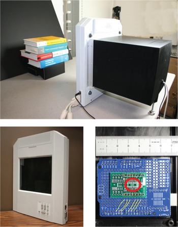
The LCD panel is configured to display 302 × 217 = 65 534 black or white squares. Each square represents an aperture element with transmittance of a 0 (black) or 1 (white). A Hadamard matrix of order N = 65 536 is used as sensing matrix, which allows a total number of 65 534, corresponding to the total number of pixels in the image, independent measurements to be made by each sensor. In our experiments, we only make a fractional of the total number of measurements. We express the number of measurements taken and used in reconstruction as a percentage of the total number of pixels. For example, 25% of measurements means 16 384 measurements are taken and used in reconstruction, which is a quarter of the total number of pixels, 65 534. In each experiment, a set of measurements is obtained by each sensor simultaneously. The two sensors are placed such that there is almost no vertical offset, and there is a horizontal offset of approximately 3.5 pixels.

B) Multi-view

Measurements taken from each of the two sensors are used to reconstruct an image using (9), independent of the measurements from the other sensor. The total variation [Reference Li, Jiang, Wilford and Scheutzow15] is used for the sparsifying operator W. The results are two images that can be used for 3D display of a scene, as shown in Fig. 8. The left and right images in Fig. 8 are placed so that the cross-eyed view results in the correct stereogram.

Fig. 8.

Multi-view images. Left: image reconstructed from measurements of sensor 1. Right: image reconstructed from measurements of sensor 2.

Each of the images in Fig. 8 was reconstructed using 50% of measurements.

C) Measurement increase

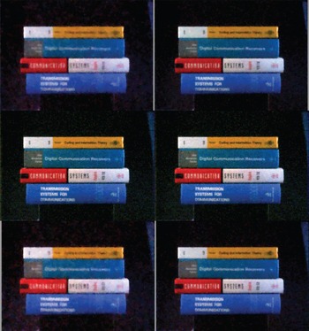
We compare the quality of images by individual and joint reconstructions in Fig. 9, which is composed of six images, arranged in two columns and three rows. On the top row, the two images are reconstructed by (9) using 12.5% (left) and 25% (right) of measurements taken from sensor 1 only. In the middle row, two images are the same; it is reconstructed by (19) using 12.5% of measurements from each of the two sensors (for a combined 25%). On the bottom row, the two images are reconstructed by (9) using 12.5% (left) and 25% (right) of measurements taken from sensor 2 only. We can make a couple of observations from Fig. 9. First, as expected, the images using 25% measurements from one sensor only are clearly better than the images using 12.5% measurements from one sensor only. That is, an image on the right column, top or bottom row, is better than an image on the left column, top or bottom row. Second, the image from joint reconstruction using measurements from both sensors is better than images using 12.5% measurements from one sensor only, and as good as the images using 25% measurements from one sensor only, i.e., in the left column, the middle image is better than top and bottom; in the right column, all three images are similar. In reconstructing the image in the middle row, although a total of 25% of measurements are used, these measurements are taken in a time interval during which each sensor only takes 12.5% of measurements.

Fig. 9.

Reconstruction using measurements from two sensors.

D) Higher resolution

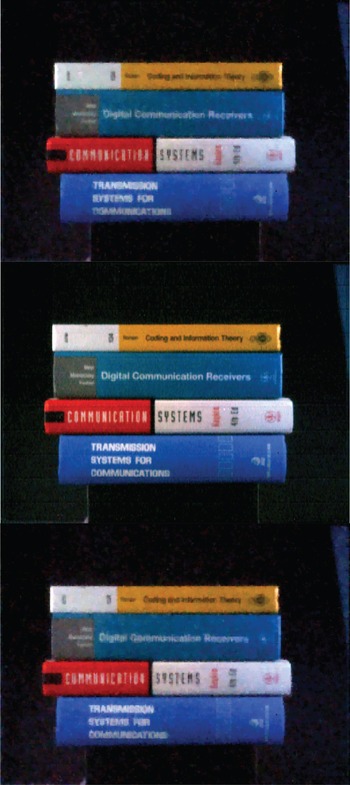
In Fig. 10, the top and bottom images are reconstructed individually by (9) using 25% of measurements taken from each of sensor 1 and sensor 2, respectively. The middle image is reconstructed using joint reconstruction to a higher resolution, 604 × 217, using 25% measurements from each of two sensors, taking the advantage that there is a 3.5 pixels horizontal offset between the two sensors. It is evident that the image in the middle is sharper due to twice the horizontal resolution.

Fig. 10.

Reconstruction to higher resolution using measurements from two sensors.