


1 Introduction
Almost every boundary layer created in an engineering or environmental context is in fact exposed to free-stream disturbances. The present numerical study considers the interaction of decaying free-stream turbulence (FST) with the fully turbulent temporal boundary layer to determine the conditions under which these free-stream disturbances are able to actively impart change upon the boundary layer.
A boundary layer developing under a free stream laden with disturbances will tend to exhibit increased skin friction and mass or heat transfer (Blair Reference Blair1983a). Considerable effort (Hancock & Bradshaw Reference Hancock and Bradshaw1983; Blair Reference Blair1983b; Castro Reference Castro1984) has thus been made to correlate observed increases in skin friction coefficient  $C_{f}$ and mass (or heat) transfer coefficient $St$ to parameters of the FST and the boundary layer. Detailed statistics have been reported by previous workers, yet are generally given at a limited number of downstream locations in an experimental facility (Nagata, Sakai & Komori Reference Nagata, Sakai and Komori2011; Sharp, Neuscamman & Warhaft Reference Sharp, Neuscamman and Warhaft2009; Dogan, Hanson & Ganapathisubramani Reference Dogan, Hanson and Ganapathisubramani2016). The current methodology is able to observe the entire interaction as it unfolds and seeks to advance our understanding of the boundary layer–FST interaction via detailed direct numerical simulation (DNS).
To date, the problem of the boundary layer developing under FST has been principally investigated experimentally. The DNS of a fully turbulent boundary layer developing under FST is an expensive undertaking that precludes systematic studies. When simulating a turbulent boundary layer with a quiescent free stream, a stretched grid is typically used far away from the wall-bounded turbulent flow. The present physical problem demands adequate resolution of the free stream with its disturbances. Previous numerical investigations have generally made use of either large-eddy simulation (e.g. Li, Schlatter & Henningson Reference Li, Schlatter and Henningson2010; Péneau, Boisson & Djilali Reference Péneau, Boisson and Djilali2000) or DNS with modest Reynolds numbers (the study of Xia et al. (Reference Xia, Ito, Nagata, Sakai, Suzuki, Terashima and Hayase2014) achieved a final momentum thickness Reynolds number  $Re_{\unicode[STIX]{x1D703}}\approx 250$). Yet there have been many studies considering the transition of an incoming laminar boundary layer under FST (Brandt, Schlatter & Henningson Reference Brandt, Schlatter and Henningson2004; Hack & Zaki Reference Hack and Zaki2014; Kreilos et al. Reference Kreilos, Khapko, Schlatter, Duguet, Henningson and Eckhardt2016). Nominally a transitional study, Wu et al. (Reference Wu, Moin, Wallace, Skarda, Lozano-Durán and Hickey2017) nevertheless achieved a final $Re_{\unicode[STIX]{x1D70F}}\approx 1000$ for a relatively weak inlet turbulence of 3 % of the mean free-stream velocity. Recently, You & Zaki (Reference You and Zaki2019) presented a DNS of a spatially developing boundary layer over the range $Re_{\unicode[STIX]{x1D703}}=1200{-}3200$ for an incoming turbulence intensity of 10 %.
Hancock & Bradshaw (Reference Hancock and Bradshaw1989) suggested that the relative fluctuating strain rate between FST and boundary layer was an important quantity to characterise their interaction. Formed from the large-eddy length scales and velocity scales of the respective flows, it may be recast as the relative large-eddy turnover time scale between the FST and boundary layer, evolving as the boundary layer grows and the unforced free-stream disturbances decay. A natural opportunity to study the evolving relative large-eddy time scale of the current physical problem is provided by the temporal framework. Kozul, Chung & Monty (Reference Kozul, Chung and Monty2016) demonstrated that the temporal boundary layer is a good model for the incompressible spatially developing turbulent boundary layer both analytically and via comparison of various statistics between the spatial and temporal boundary layers. Additionally, under a quiescent free stream, the mean entrainment of non-turbulent fluid by the turbulent temporal boundary layer  $E=\text{d}\unicode[STIX]{x1D6FF}/\text{d}t=U_{\infty }\,\text{d}\unicode[STIX]{x1D6FF}/\text{d}X$ (where $\unicode[STIX]{x1D6FF}$ is the boundary layer thickness, $U_{\infty }$ is the free-stream velocity and $X=U_{\infty }t$ for time $t$) is not unlike the process in a turbulent spatial boundary layer $E=U_{\infty }\,\text{d}\unicode[STIX]{x1D6FF}/\text{d}x-W_{\unicode[STIX]{x1D6FF}}$ (where $W_{\unicode[STIX]{x1D6FF}}$ is the mean wall-normal velocity at the edge of the boundary layer). The difference in mean entrained fluid is due only to the small $W_{\unicode[STIX]{x1D6FF}}$ in the spatial boundary layer that vanishes at large Reynolds number. Thus the temporal boundary layer will capture the finite, non-vanishing part of the entrainment in the asymptotic limit of the spatial boundary layer, i.e. $E\rightarrow 0.22\,U_{\unicode[STIX]{x1D70F}}$, where $U_{\unicode[STIX]{x1D70F}}$ is the friction velocity (cf. coefficients $a_{2}$ and $b_{2}$ in figure 18 of Kozul et al. (Reference Kozul, Chung and Monty2016)). The Reynolds numbers of the present simulations, although in the fully turbulent regime, clearly fall short of this asymptotic limit. The current temporal model is therefore a potential source of inaccuracy if direct comparison of the entrainment to that of the spatial boundary layer is sought.
The efficiency of the temporal framework, which employs a streamwise-shortened domain, allows us to mitigate some of the cost associated with this demanding physical problem. Whilst a wide-ranging scan of length scales and intensities would be ideal to determine the roles of each in the interaction with the boundary layer, in practice we are limited to cases where the free-stream length scale is a small multiple of the boundary layer thickness. The integral length scale of the FST, growing as its intensity decays in time, must remain much smaller than the domain size such that the associated large-scale energy-carrying eddies evolve freely (Thornber Reference Thornber2016). A simulation where the large-eddy length scale of the FST is much larger than that of the boundary layer thickness is untenable given present computational capabilities: it would require the vast majority of the domain, that is, available computational resources, to be dedicated to simulating the FST, when our primary concern here is its interaction with the boundary layer. In fact, the response of the boundary layer to small-scale turbulence in the free stream remains rather under-explored compared to that of large-scale FST (Nagata et al. Reference Nagata, Sakai and Komori2011). Nevertheless, the present efficient temporal framework permits a limited parametric investigation of this costly physical problem. In addition to exposing a boundary layer to FST from its inception, the present work gains access to other regimes by adding or injecting homogeneous isotropic turbulence (HIT) to the free stream of boundary layers already grown to a desired thickness in a quiescent free stream. Such an approach making use of synthesised fields was previously used for wakes developing under free-stream disturbances (Rind & Castro Reference Rind and Castro2012).
Since many engineering problems feature turbulent boundary layers exposed to ambient free-stream conditions that cannot realistically be considered laminar, our work helps to clarify when and how such free-stream disturbances could, via active manipulation, alter the form and development of boundary layers forming over walls. The present parametric study of (wall-bounded) shear flow with FST complements previous systematic numerical campaigns concerning shear flows subject to free-stream disturbances, including wakes (Rind & Castro Reference Rind and Castro2012), stratified wakes (Pal & Sarkar Reference Pal and Sarkar2015) and shear layers (Kaminski & Smyth Reference Kaminski and Smyth2019). We show how the relative large-eddy turnover time scale indicates whether there will be a ‘strong’ or ‘weak’ interaction between the two flows. If the large-eddy turnover time scale of the boundary layer is less than approximately twice that of the FST, the free-stream disturbances will have time to impart change on the boundary layer before the FST fades away. From the boundary layer’s point of view, it needs time to adjust to the FST via ingestion of the inactive motions from the free stream. Significant changes to the boundary layer eventuate only if the FST is still relatively strong by the time this occurs. Previous equilibrium approaches have attempted parametrisation using physical quantities at a single point in space or time. In contrast, the present temporal simulations expose the inherent developing nature of this physical problem.
2 Velocity and length scales of the boundary layer–FST problem
Sketch of the physical problem: a turbulent temporal boundary layer developing under decaying FST. The set-up employs a periodic boundary condition in the streamwise direction.
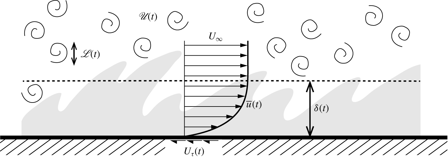
The FST to which boundary layers are often exposed will herein be modelled as HIT. The large scales of this HIT will be characterised by a velocity scale ( $\mathscr{U}$) and an integral length scale ( $\mathscr{L}$). Figure 1 sketches the physical problem within the temporal framework. Such an approach is particularly suited to the problem since the evolution of HIT is classically described by temporal decay, and the boundary layer being recast thus (Kozul et al. Reference Kozul, Chung and Monty2016) allows us to directly compare the evolution of the relative large-eddy turnover time scales of the two flows.
To parametrise our physical problem, we estimate how these scales of the HIT evolve with respect to the relevant velocity scale (friction velocity  $U_{\unicode[STIX]{x1D70F}}$) and large-eddy length scale ( $\unicode[STIX]{x1D6FF}$; for 99 % boundary layer thickness $\unicode[STIX]{x1D6FF}\equiv \unicode[STIX]{x1D6FF}_{99}$, computed from the mean streamwise velocity profile) of the boundary layer. Whether the large scales in decaying HIT are described by the Batchelor or Saffman theories of turbulence is a long-standing debate not entered into by the present work. The following relations are only of interest here as we endeavour to establish how the scales of the boundary layer and FST would evolve with respect to each other assuming no interaction between them. It is generally agreed (e.g. Krogstad & Davidson Reference Krogstad and Davidson2010) that both $\mathscr{U}$ and $\mathscr{L}$ evolve temporally according to power laws; the two classical theories suggest differing exponents. In the Batchelor (Reference Batchelor1953) theory, integral scales $\mathscr{U}$ and $\mathscr{L}$ satisfy $\mathscr{U}^{2}\mathscr{L}^{5}=\text{constant}$, and when combined with the empirical relation
 $$\begin{eqnarray}\frac{\text{d}\mathscr{U}^{2}}{\text{d}t}=-A\frac{\mathscr{U}^{3}}{\mathscr{L}},\end{eqnarray}$$
 for some constant  $A$, the decay law $\mathscr{U}^{2}\sim t^{-10/7}$ (and associated $\mathscr{L}\sim t^{2/7}$) results. The theory due to Saffman (Reference Saffman1967) predicts the group $\mathscr{U}^{2}\mathscr{L}^{3}=\text{constant}$ which gives $\mathscr{U}^{2}\sim t^{-6/5}$ (and $\mathscr{L}\sim t^{2/5}$). The two classical types of turbulence are associated with specific forms of the energy spectrum $E$: for the Batchelor type $E(\unicode[STIX]{x1D705}\rightarrow 0)\sim \unicode[STIX]{x1D705}^{4}$ for wavenumber $\unicode[STIX]{x1D705}$, whereas Saffman turbulence has the spectrum $E(\unicode[STIX]{x1D705}\rightarrow 0)\sim \unicode[STIX]{x1D705}^{2}$. Which form of turbulence is exhibited, and importantly what value of decay rate arises, depends upon initial conditions (Lavoie, Djenidi & Antonia Reference Lavoie, Djenidi and Antonia2007; Antonia et al. Reference Antonia, Lee, Djenidi, Lavoie and Danaila2013; Hearst & Lavoie Reference Hearst and Lavoie2016), but it would appear that the turbulence retains the spectrum (either ${\sim}\unicode[STIX]{x1D705}^{2}$ or ${\sim}\unicode[STIX]{x1D705}^{4}$) with which it was created (Ishida, Davidson & Kaneda Reference Ishida, Davidson and Kaneda2006). The decay exponent of classic grid turbulence appears to be closer to that suggested by the Saffman spectrum (Krogstad & Davidson Reference Krogstad and Davidson2010), a conclusion consistent with DNS of temporal grid turbulence (Watanabe & Nagata Reference Watanabe and Nagata2018). Both $E\sim \unicode[STIX]{x1D705}^{2}$ (Huang & Leonard Reference Huang and Leonard1994; Mansour & Wray Reference Mansour and Wray1994) and $E\sim \unicode[STIX]{x1D705}^{4}$ (Ishida et al. Reference Ishida, Davidson and Kaneda2006; Thornber Reference Thornber2016) energy spectra have been used to initialise the flow fields of numerical simulations.
The choice of a velocity scale  $\mathscr{U}$ for the FST is usually set to be the streamwise root-mean-squared velocity fluctuations $u_{e}^{\prime }$, for comparison to experiments; however, since our HIT is perfectly isotropic any velocity component could have been chosen. The choice of a suitable length scale is rather less obvious. A length scale $L_{e}^{u}$ was defined by Hancock & Bradshaw (Reference Hancock and Bradshaw1983) as
 $$\begin{eqnarray}U_{\infty }\frac{\text{d}(u_{e}^{\prime })^{2}}{\text{d}X}\equiv \frac{-(u_{e}^{\prime })^{3}}{L_{e}^{u}},\end{eqnarray}$$
 for mean streamwise free-stream velocity  $U_{\infty }$ and distance from the turbulence-producing grid $X$. Several alternative definitions for the energy-carrying integral length scale of HIT have been offered in the literature. A common definition is the value of the integrated normalised autocorrelation to the first zero crossing, $r_{0}$:
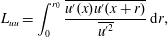 $$\begin{eqnarray}L_{uu}=\int _{0}^{r_{0}}\frac{\overline{u^{\prime }(x)u^{\prime }(x+r)}}{\overline{u^{\prime 2}}}\,\text{d}r,\end{eqnarray}$$
 as used in Hearst, Dogan & Ganapathisubramani (Reference Hearst, Dogan and Ganapathisubramani2018) for example. However, this quantity can be problematic since this zero crossing is somewhat elusive (Dogan et al. Reference Dogan, Hanson and Ganapathisubramani2016). The non-dimensional dissipation rate ( $C_{\unicode[STIX]{x1D700}}=\unicode[STIX]{x1D700}L_{uu}/u_{e}^{\prime }$) for the current forced HIT is $C_{\unicode[STIX]{x1D700}}\approx 0.5$, in agreement with the spread of values found for forced HIT in the survey of Kaneda et al. (Reference Kaneda, Ishihara, Yokokawa, Itakura and Uno2003). When forcing is turned off within the triply periodic domain, $C_{\unicode[STIX]{x1D700}}$ gradually increases over $t\approx 2\,T_{e,0}$ to $C_{\unicode[STIX]{x1D700}}\approx 1.8$ (where $Re_{\unicode[STIX]{x1D706}}=u^{\prime }\unicode[STIX]{x1D706}/\unicode[STIX]{x1D708}$ is decreasing and is ${\approx}30$ at this point). However, this value for the dissipation rate is neither well-converged nor particularly reliable, since at this later time the growing integral length scale $L_{uu}$ exceeds 10 % of the smallest box dimension. For perfectly isotropic turbulence, the length scale $L_{e}^{u}$ from (2.2) can be written as
 $$\begin{eqnarray}L_{e}^{u}=\frac{3}{2}\,\frac{(u_{e}^{\prime })^{3}}{\unicode[STIX]{x1D700}},\end{eqnarray}$$
 for kinetic energy dissipation rate  $\unicode[STIX]{x1D700}\equiv \unicode[STIX]{x1D708}\overline{(\unicode[STIX]{x2202}u_{i}^{\prime }/\unicode[STIX]{x2202}x_{j})^{2}}$ with kinematic viscosity $\unicode[STIX]{x1D708}$. However, as pointed out in Hearst et al. (Reference Hearst, Dogan and Ganapathisubramani2018), associating this dissipation-derived quantity with a length scale actually existing in the flow is not always a valid undertaking. Our present use of (2.4) to derive a relevant length scale does not suggest we have an equilibrium state during the decaying phase, as (2.2) assumes. Rather we use it to avoid the ambiguity associated with $L_{uu}$ due to a limited domain size. We use the term ‘large-eddy length scale’ throughout when referring to that of the FST since we are most commonly comparing it to the ‘large-eddy length scale’ of the boundary layer, $\unicode[STIX]{x1D6FF}$ (indeed we will most frequently refer to the ‘large-eddy length scale ratio’, $L_{e}^{u}/\unicode[STIX]{x1D6FF}$). We formally refer to $L_{uu}$ as the ‘integral length scale’. The dissipation-based $L_{e}^{u}$ is taken as being representative of large eddies in the FST since it is well defined for restricted numerical domains and dissipation-based length scales are commonly used (e.g. You & Zaki Reference You and Zaki2019). Later in this work it is shown that using either the dissipation-based $L_{e}^{u}$ from (2.4) or a length scale based on a velocity autocorrelation as per (2.3) does not alter our main conclusions.
We seek to estimate the evolution of the relative large-eddy turnover time scales for the boundary layer–FST problem. The behaviour of our HIT lies somewhere between the two classical models (the evolution of the defined velocity and length scales for the HIT is shown later in figure 3). We note the large-eddy turnover time scale of the HIT evolves as  $T_{e}=\mathscr{L}/\mathscr{U}\sim t$ for both the Saffman ( $t^{2/5}/t^{-3/5}\sim t$) and Batchelor ( $t^{2/7}/t^{-5/7}\sim t$) theories, meaning the following analysis is the same irrespective of the type of HIT exhibited. White (Reference White2006) (equation 6-70) offers simple empirical power-law relations for turbulent boundary layers forming over flat plates, such that we can write $\unicode[STIX]{x1D6FF}\sim t^{6/7}$ by using $X=U_{\infty }t$, that is, the boundary layer is scaled by an observer travelling with the free stream. Temporal development as $U_{\unicode[STIX]{x1D70F}}\sim t^{-1/7}$ is consistent with a constant boundary layer spreading rate $(1/U_{\unicode[STIX]{x1D70F}})(\text{d}\unicode[STIX]{x1D6FF}/\text{d}t)$ (figure 8d). However, we note the relations of White (Reference White2006) suggest $U_{\unicode[STIX]{x1D70F}}\sim t^{-1/14}$. The present problem makes use of boundary layers that have been ‘pre-grown’ to a certain thickness prior to HIT injection into the free stream. Thus their development in time is advanced with respect to that of the HIT by $t_{0}$, the time at HIT injection into the free stream. Armed with indicative power-law relations for the velocity and large-eddy length scales pertaining to the HIT (forming our FST) and that of the boundary layer, we estimate the evolution of the relative large-eddy turnover time scales for our present problem at large $t$ as a simple power law:
 $$\begin{eqnarray}e\equiv \frac{T_{\unicode[STIX]{x1D6FF}}}{T_{e}}=\frac{\unicode[STIX]{x1D6FF}/U_{\unicode[STIX]{x1D70F}}}{L_{e}^{u}/u_{e}^{\prime }}\sim \frac{t^{6/7}/t^{-1/7}}{t}\sim \frac{t}{t}\sim \text{constant}.\end{eqnarray}$$
 Thus, for the estimated power-law evolution of our individual parameters, at large  $t$, this ratio will tend to remain constant if the boundary layer and FST do not interact. The time evolution of the numerator is perhaps ‘not very accurate’ (White Reference White2006); however, in this context it nonetheless permits an estimate of the relative evolution of the boundary layer with respect to the HIT. The exponent for the quiescent temporal boundary layer of Kozul et al. (Reference Kozul, Chung and Monty2016) ranges ${\approx}[0.71,0.73]$ (compared to $6/7\approx 0.86$), and that for $U_{\unicode[STIX]{x1D70F}}$ is found to be ${\approx}[-0.089,-0.083]$ (versus $-1/7\approx 0.14$ or $-1/14\approx -0.071$). The significance of the above estimate is that $e$ approaches a constant at large $t$ for non-interacting boundary layer and HIT flows. As we will show later, a ‘strong’ interaction occurs if this parameter is less than around 2 at the moment when the boundary layer is first exposed to the FST. This same quantity was interpreted as a relative fluctuating strain rate by Hancock & Bradshaw (Reference Hancock and Bradshaw1989) as mentioned in § 1. The aim of the present work is to argue the importance of $e$ from the view of relative lifetimes in explaining potential boundary layer modification by FST. This is in addition to the better understood necessary minimum external turbulence level.
3 Simulation set-up
Hereafter, we refer to fluctuating velocities  $u$,
$u$,  $v$ and $w$ in the $x$ (streamwise), $y$ (spanwise) and $z$ (wall-normal) directions. The appropriate Reynolds decomposition for the temporally developing turbulent boundary layer is given by $u_{i}=\overline{u}(z,t)\unicode[STIX]{x1D6FF}_{i1}+u_{i}^{\prime }(x,y,z,t)$, where $\overline{(\cdot )}$ indicates averaging in the homogeneous $xy$ planes. Statistics throughout the present work are computed at instantaneous times (i.e. from single velocity and scalar fields) and corresponding instantaneous FST statistics (i.e. $u_{rms}^{\prime }$ and $L_{e}^{u}$) are quoted. This is in contrast to the time window averaging used for the quiescent boundary layer in Kozul et al. (Reference Kozul, Chung and Monty2016). The simulations presented herein are all single realisations meaning only moderate statistical convergence is achieved.
3.1 Generation of free-stream disturbances: HIT
The previously quiescent free stream of the turbulent temporal boundary layer is now seeded with HIT generated in a triply periodic domain in a precursor simulation using the spectral code of Chung & Matheou (Reference Chung and Matheou2012) (shear turned off). A Fourier pseudospectral method (cf. Rogallo Reference Rogallo1981) is used to integrate the Navier–Stokes equations, whose solution is advanced in time using the low-storage third-order Runge–Kutta scheme of Spalart, Moser & Rogers (Reference Spalart, Moser and Rogers1991). Quantities external to the boundary layer are identified with subscript  $e$, and values at the beginning of the combined boundary layer–FST simulations with subscript $0$. The cases will be characterised by a FST intensity $u_{e}^{\prime }/U_{\unicode[STIX]{x1D70F}}$, where $u_{e}^{\prime }$ is the isotropic root-mean-squared velocity fluctuations of the HIT. The large-eddy length scale ratio is $L_{e}^{u}/\unicode[STIX]{x1D6FF}$.
One-dimensional spectrum of the current FST cases both (a) uncompensated and (b) compensated: ——, current HIT field used to form the FST at  $t=0$ for all cases except A1 (table 1) with $Re_{\unicode[STIX]{x1D706},0}=82$;
  ,
,  $Re_{\unicode[STIX]{x1D706}}=99$ case of Mydlarski & Warhaft (Reference Mydlarski and Warhaft1996); – – –, line at 0.5, the expected plateau value for the compensated spectrum within the scaling or inertial subrange region for high-Reynolds-number turbulence. Vertical grey band indicates the forced region in radial wavenumber range, keeping in mind that all $\unicode[STIX]{x1D705}_{x}<\unicode[STIX]{x1D705}_{f}$ are forced since the one-dimensional spectrum is aliased.
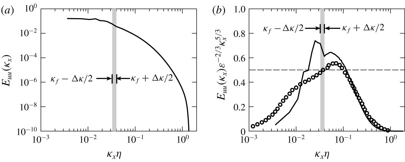
Figure 2 shows both the uncompensated and the compensated streamwise-velocity one-dimensional spectra for the HIT field used to form the FST for all present simulations (except case A1). The observed peak is due to our forcing at a fixed shell of wavenumbers. Our HIT possesses only a limited region where the turbulence might be approximately inertial. Despite being modest, the present Taylor Reynolds numbers of the HIT still admit power-law decay of the kinetic energy. A time interval  ${\approx}T_{e,0}$ is required before $u_{e}^{\prime }$ of the HIT begins this power-law decay.
(a) Decaying turbulence velocity scale  $\mathscr{U}\rightarrow u_{e}^{\prime }$ with fits $(u_{e}^{\prime })^{2}/(u_{e,0}^{\prime })^{2}=$ $(1+a_{u_{e}^{\prime }}t/T_{e,0})^{b}$ following Krogstad & Davidson (Reference Krogstad and Davidson2010): ——, Saffman-type turbulence with $b=-6/5$; – – –, Batchelor-type turbulence with $b=-10/7$; constant $a_{u_{e}^{\prime }}=2.3$ for both. (b) Growing length scale $\mathscr{L}\rightarrow L_{e}^{u}$ (2.4) formed from fits for $u_{e}^{\prime }$ as in (a) and $\unicode[STIX]{x1D700}_{e}/\unicode[STIX]{x1D700}_{e,0}=(1+a_{\unicode[STIX]{x1D700}_{e}}t/T_{e,0})^{b-1}$ for dissipation in the free-stream $\unicode[STIX]{x1D700}_{e}$ (not shown), constant $a_{\unicode[STIX]{x1D700}_{e}}=1.3$ for both, curves as for (a): —— (teal), in the free stream of case D (table 2);
  , decay in the box turbulence code. Dimension $L_{z}=L_{y}$ $=L_{x}/2$ is the smallest box dimension for the simulations. Subscript $e$ denotes quantities external to the boundary layer and subscript $0$ values at the beginning of the combined boundary layer–FST simulations. Here $T_{e,0}=L_{e,0}^{u}/u_{e,0}^{\prime }$ is the large-eddy turnover time scale of the forced statistically steady HIT.
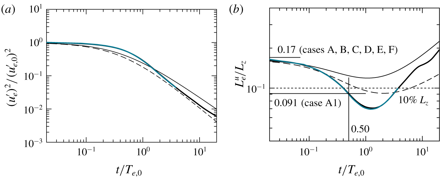
Table 1 provides the main parameters for the precursor HIT simulations. A desired  $L_{e,0}^{u}$ in the FST is achieved via forcing to a selected shell of wavenumbers at constant power (similar to that in Carati, Ghosal & Moin (Reference Carati, Ghosal and Moin1995)), centred on forcing wavenumber $\unicode[STIX]{x1D705}_{f}$. For the present HIT, $\unicode[STIX]{x1D705}_{f}L_{e,0}^{u}\approx 5$ with forcing shell thickness $\unicode[STIX]{x0394}\unicode[STIX]{x1D705}\,L_{e,0}^{u}\approx 1$. The ranges of relative length ( $L_{e}^{u}/\unicode[STIX]{x1D6FF}$) and velocity ( $u_{e}^{\prime }/U_{\unicode[STIX]{x1D70F}}$) scale ratios are extended by injecting the HIT into the free stream of boundary layers that had been ‘pre-grown’ to different thicknesses $\unicode[STIX]{x1D6FF}$, or equivalently, Reynolds numbers. The HIT kinetic energy decays according to established power laws as detailed above in § 2 and care was taken to ensure the domain size did not constrict this behaviour. In simulations of decaying HIT, estimates of the integral length scale may become unreliable if it approaches a significant fraction the smallest domain dimension, primarily due to a lack of statistical averaging (Thornber Reference Thornber2016). The present simulations use an $L_{e}^{u}$ that is maximally 17 % of the smallest domain dimension at the time of insertion into the free stream, when it then decays for $t\approx T_{e,0}$, where $T_{e,0}=L_{e,0}^{u}/u_{e,0}^{\prime }$ is the large-eddy turnover time scale of the forced steady-state HIT, before beginning power-law growth. Although figure 3(b) suggests this power-law growth is not seriously impeded up to $L_{e}^{u}\approx 0.2\,L_{z}$, the simulations are conservatively halted when $L_{e}^{u}\approx 0.1\,L_{z}$, following the observations of Thornber (Reference Thornber2016). At the moment of injection into the free stream, the Taylor Reynolds number of the FST is $Re_{\unicode[STIX]{x1D706},0}=u_{e,0}^{\prime }\unicode[STIX]{x1D706}_{e,0}/\unicode[STIX]{x1D708}\approx 82$, for Taylor microscale $\unicode[STIX]{x1D706}$, for all present cases except A1 (table 1), for which it is $Re_{\unicode[STIX]{x1D706},0}\approx 52$. Forcing to the HIT is removed at the moment of injection into the boundary layer’s free stream such that the HIT fields begin decaying as the simulations with synthesised initial conditions are launched.
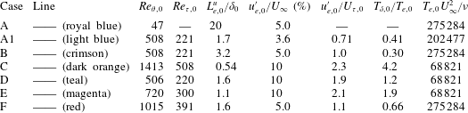
Parameters for the precursor HIT simulations that formed the FST fields once inserted into the free stream of the cases listed in table 2. Physical quantities correspond to values at  $t=0$ (denoted with subscript $0$) and external (subscript $e$) to the boundary layer in the simulations of table 2. Parameter $Re_{\mathscr{L}}=L_{e}^{u}u_{e}^{\prime }/\unicode[STIX]{x1D708}$ is the turbulent Reynolds number of the HIT formed using the dissipation length scale $L_{e}^{u}$ as the large-eddy length scale $\mathscr{L}$. Length scales are noted as a fraction of $L_{z}=L_{y}$ being the smallest and thus limiting domain dimension. Wavenumber $\unicode[STIX]{x1D705}_{c,max}$ is the cutoff wavenumber for the present HIT simulations. Cases A to F are at steady state and forced until the moment of insertion into the free stream of the boundary layers. The HIT case for case A1 is simply that of the first row but allowed to decay for $0.50\,T_{e,0}$ within the triply periodic box turbulence code by removing the forcing.

Case A1 is a companion simulation to case A: the HIT injected into the free stream of case A1 at  $Re_{\unicode[STIX]{x1D703}}=508$ is identical to the HIT in the free stream of case A (where the boundary layer is ‘born’ under FST) at that same $Re_{\unicode[STIX]{x1D703}}$. Any difference between cases A and A1 is therefore due to their differing development histories. That is, HIT for case A1 is that for case A (and all others) yet allowed to decay (by removing the forcing) within the precursor HIT simulation for $0.50\,T_{e,0}$ before injection, being the same interval of time required by the boundary layer of case A, exposed to the HIT from inception, to reach $Re_{\unicode[STIX]{x1D703}}\approx 500$. Hence all combined boundary layer–FST simulations (table 2) presented herein made use of only one forced HIT case. Case A1 is then formed by inserting the partially decayed HIT over a boundary layer formed under a quiescent free stream with $Re_{\unicode[STIX]{x1D703}}\approx 500$. This permitted investigation of the ‘recovery’ time required following the artificial combination of the fields (§ 3.2), that is, to gauge the difference between our cases formed from artificially synthesised fields and a boundary layer that has begun life under FST.
3.2 Combined simulations: the boundary layer is seeded with FST
Parameters of the present simulations of boundary layers developing under decaying FST. The turbulence intensity relative to the constant free-stream velocity is given by  $Tu_{0}\equiv u_{e,0}^{\prime }/U_{\infty }$. Different values of $L_{e,0}^{u}/\unicode[STIX]{x1D6FF}_{0}$ are achieved by introducing the HIT into the free stream of a temporal boundary layer developing in a quiescent field at various $Re_{\unicode[STIX]{x1D703}}=U_{\infty }\unicode[STIX]{x1D703}/\unicode[STIX]{x1D708}$, with momentum thickness $\unicode[STIX]{x1D703}$. A significant difference in intensities $u_{e,0}^{\prime }/U_{\infty }$ was achieved by changing $U_{\infty }$ by a factor of 2 (i.e. cases A, A1, B, F versus cases C, D, E). Here $T_{\unicode[STIX]{x1D6FF}}=\unicode[STIX]{x1D6FF}/U_{\unicode[STIX]{x1D70F}}$ is the boundary layer large-eddy turnover time scale. Case A1 is a companion simulation to case A where we allow the HIT for case A1 to decay for $0.50\,T_{e,0}$ before injection, being the same interval of time required by the boundary layer of case A, exposed to the HIT from inception, to reach $Re_{\unicode[STIX]{x1D703}}=508$. Note the large difference in $T_{\unicode[STIX]{x1D6FF},0}/T_{e,0}=e_{0}$ between cases C and D: the boundary layer was ‘pre-grown’ to a higher Reynolds number in case C before the FST was added. It therefore has a much larger large-eddy turnover time scale than case D, and also compared to that of the FST. The friction velocity $U_{\unicode[STIX]{x1D70F},0}$ for case A at FST injection (which is when the boundary layer also starts growing) is non-physical due to the numerical trip used. Moreover the relative large-eddy turnover time $e\equiv T_{\unicode[STIX]{x1D6FF}}/T_{e}$ is formed from scales that characterise the fully turbulent (i.e. inertial) boundary layer and the HIT, and thus is not here used to gauge interaction between a transitioning boundary layer ( $Re_{\unicode[STIX]{x1D703}}<500$ for the present temporal boundary layers) and HIT.
The finite-difference code used for both the ‘pre-grown’ boundary layers and the synthesised fields for which statistics are presented herein has been validated in Kozul et al. (Reference Kozul, Chung and Monty2016). The code employs the fully conservative fourth-order staggered finite-difference scheme of Verstappen & Veldman (Reference Verstappen and Veldman2003) to spatially discretise the Navier–Stokes equations, with the boundary conditions of Sanderse, Verstappen & Koren (Reference Sanderse, Verstappen and Koren2014). As for the precursor HIT simulations, the solution is marched forward in time using the low-storage third-order Runge–Kutta scheme of Spalart et al. (Reference Spalart, Moser and Rogers1991). The fractional-step method (e.g. Perot Reference Perot1993) is used after each substep to project the velocity onto a divergence-free space, ensuring satisfaction of the continuity equation. Grid points are clustered near the wall using an error function stretching set by  $z(\unicode[STIX]{x1D709})=\text{erf}[a(\unicode[STIX]{x1D709}-1)]/\text{erf}(a)$ for $a\approx 2$ and
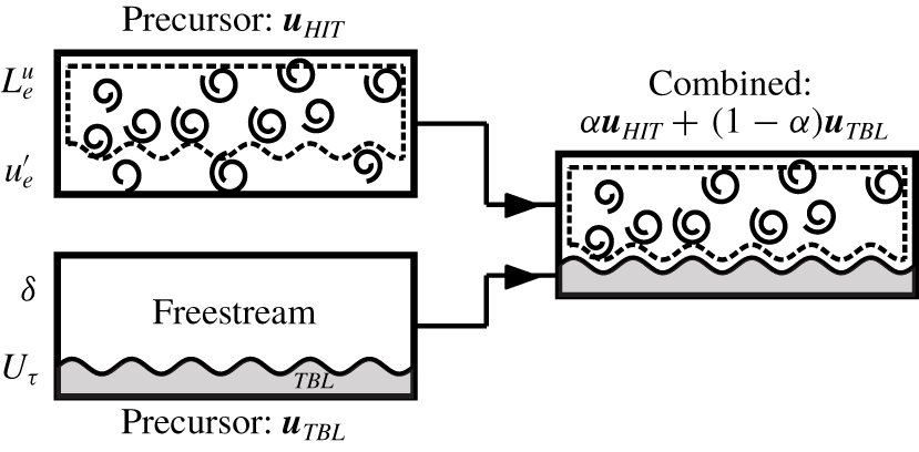
  $\unicode[STIX]{x1D709}=[0,1]$ (Pirozzoli, Bernardini & Orlandi Reference Pirozzoli, Bernardini and Orlandi2016). The HIT and boundary layer velocity fields are combined via thresholding on the passive scalar $c$ with Schmidt number $Sc=1$, taking a value of $C_{w}$ at the wall. It is here used as a proxy for the extent of boundary layer growth into the domain since $c$ is initially at the free-stream (top boundary) value $C_{\infty }$ everywhere. In contrast, the simulations of Rind & Castro (Reference Rind and Castro2012) and Pal & Sarkar (Reference Pal and Sarkar2015) embedded wakes in HIT based on criteria relating to the velocity field. The present approach is more akin to the experiments of Hancock & Bradshaw (Reference Hancock and Bradshaw1989), where the boundary layer developed over a slightly heated plate, allowing the wall-generated turbulence to be distinguished from the FST via an appropriate temperature threshold. The present simulations employ a passive scalar released at the wall for the same purpose, serving to ‘mark’ fluid originating in the boundary layer. Therefore we are able to assess the mixing of one flow (the turbulent boundary layer) with another (the HIT) by adopting a similar thresholding approach, rather than inferring the extent of mixing from the velocity or vorticity fields. We are thus able to attribute the turbulent fluid’s origin with some confidence, as opposed to relying on the velocity field, which is non-local due to the incompressible pressure condition. The present approach also eliminates the possibility of a bias towards any one component of velocity. Several recent studies have shown reliable demarcation of wall-generated turbulence from the free stream based on a passive scalar threshold (compared to one based on vorticity magnitude) both without (Watanabe, Zhang & Nagata Reference Watanabe, Zhang and Nagata2018) and with (Wu, Wallace & Hickey Reference Wu, Wallace and Hickey2019) FST. Using a threshold based on the kinetic energy was shown to incur the largest error in identifying the turbulent–non-turbulent interface in the study of Watanabe et al. (Reference Watanabe, Zhang and Nagata2018). The HIT is first interpolated using cubic splines onto the stretched grid required by the temporal boundary layer simulation. A function effectively masking the HIT by the turbulent boundary layer then gives the combined field $\boldsymbol{u}_{0}=\unicode[STIX]{x1D6FC}\boldsymbol{u}_{HIT}+(1-\unicode[STIX]{x1D6FC})\boldsymbol{u}_{TBL}$ with
 $$\begin{eqnarray}\unicode[STIX]{x1D6FC}(\boldsymbol{x})=\left\{\begin{array}{@{}ll@{}}0,\quad & 0\leqslant \displaystyle \frac{C_{w}-c}{C_{w}-C_{\infty }}\leqslant 0.95\\ 1,\quad & 0.95<\displaystyle \frac{C_{w}-c}{C_{w}-C_{\infty }}\leqslant 1,\end{array}\right.\end{eqnarray}$$
 for  $\boldsymbol{x}=(x,y,z)$ and $\boldsymbol{u}=(u,v,w)$, for scalar contrast $C_{w}-C_{\infty }$. Figure 4 shows a schematic of this field combination. All cases except case A are formed thus; for case A the HIT fields form the entire initial velocity fields (with a numerical trip imposed at the wall). Case A is thus analogous to most previous experimental studies of the present physical problem, where the boundary layer is exposed to FST from the beginning of its development. The scalar field is unchanged during the synthesis of the velocity fields (i.e. no fluctuations are added to the scalar field). The artificially synthesised (patched) initial fields are not divergence-free as required by the continuity equation; however, this is corrected after a single time step, when the numerical scheme employed projects the flow onto a divergence-free space. Physical quantities for the present cases are given in table 2. Importantly the final column notes $e_{0}=T_{\unicode[STIX]{x1D6FF},0}/T_{e,0}=(\unicode[STIX]{x1D6FF}/U_{\unicode[STIX]{x1D70F}})_{0}/(L_{e}^{u}/u_{e}^{\prime })_{0}$, the initial relative large-eddy turnover time scale between the turbulent boundary layer and the FST. When the fields are combined, a decrease ( ${\approx}9\,\%$ for cases A1, B and F; ${\approx}11\,\%$ for cases D and E; and ${\approx}6\,\%$ for case C) in $\unicode[STIX]{x1D6FF}$ results at the first time step post-HIT injection; values of $\unicode[STIX]{x1D6FF}_{0}$ (and therefore $e_{0}$ at $t=0$) correspond to that before the HIT injection. No such change occurs in $U_{\unicode[STIX]{x1D70F}}$.
Periodic boundary conditions are imposed in the streamwise direction  $x$ as well as the spanwise direction $y$. A ‘conveyor-belt’ moving-wall set-up is used in the boundary layer simulations. At this bottom wall where $z=0$, $u=U_{w}$ and $v=w=0$ are imposed. The top boundary ( $z=L_{z}$) is a fixed wall with an impermeable boundary condition on the normal velocity ( $w=0$) and slip boundary conditions on velocities tangential to the upper wall ( $\unicode[STIX]{x2202}u/\unicode[STIX]{x2202}z=\unicode[STIX]{x2202}v/\unicode[STIX]{x2202}z=0$). The familiar configuration, with a stationary no-slip wall and non-zero free-stream velocity $|U_{\infty }|=|U_{w}|$, is recovered via Galilean transformation. The resolution of non-spectral discretisation schemes is improved by use of a reference frame with zero mean bulk velocity (Bernardini et al. Reference Bernardini, Pirozzoli, Quadrio and Orlandi2013). Therefore the present set-up with zero mean velocity in the free stream is the most advantageous choice for resolution of disturbances away from the wall where grid spacing is larger. An initial trip $Re_{D}\equiv DU_{w}/\unicode[STIX]{x1D708}\approx 500$, for trip height $D$, is used to trigger transition of the precursor boundary layer simulations to a turbulent regime as in Kozul et al. (Reference Kozul, Chung and Monty2016). The pressure gradient is set to zero. We use a domain where $L_{x}=2L_{y}=2L_{z}$. The simulations can be run until one of the box constraints is met: either $L_{e}^{u}\approx L_{z}/10$ (equivalently $L_{e}^{u}\approx L_{y}/10$) (Thornber Reference Thornber2016) or $\unicode[STIX]{x1D6FF}\approx L_{z}/3$ (Schlatter & Örlü Reference Schlatter and Örlü2010). Grid details for the boundary layer–FST simulations are given in table 3.
Schematic of the combined fields formed from precursor simulations via masking (3.1) using the scalar concentration of the boundary layer, represented by the grey shaded area (TBL, turbulent boundary layer).
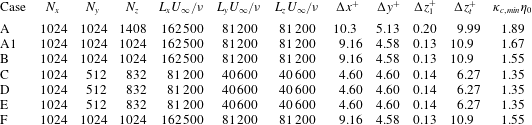
Grid details for the simulations of boundary layers developing under decaying FST. The precursor HIT simulations use a constant grid spacing in all three dimensions. For the combined boundary layer simulations, grid points are clustered near the bottom wall using an error function stretching  $z(\unicode[STIX]{x1D709})=\text{erf}[a(\unicode[STIX]{x1D709}-1)]/\text{erf}(a)$ for $a\approx 2$ and $\unicode[STIX]{x1D709}=[0,1]$ (Pirozzoli et al. Reference Pirozzoli, Bernardini and Orlandi2016). Wavenumber $\unicode[STIX]{x1D705}_{c,min}=\unicode[STIX]{x03C0}/\unicode[STIX]{x0394}z_{t}$ is the cutoff wavenumber for the largest vertical spacing in the simulation, at the top free-slip boundary, set such that $\unicode[STIX]{x1D705}_{c,min}\unicode[STIX]{x1D702}_{0}$ is comparable to, or smaller than, $\unicode[STIX]{x1D705}_{c,max}\unicode[STIX]{x1D702}_{0}$ in table 1 for the precursor HIT simulations. Note that $\unicode[STIX]{x1D705}_{c,max}\unicode[STIX]{x1D702}_{0}$ in the boundary layer simulations is at the wall. Spacing $\unicode[STIX]{x0394}z_{1}^{+}$ denotes the maximum first grid spacing at the bottom wall, whereas $\unicode[STIX]{x0394}z_{t}^{+}$ is the maximum spacing at the top wall. Cited here are the coarsest grid spacings in wall units observed over the duration of the simulation. Note that cases A1, B and F, and then cases C, D and E use the same initial boundary layer configuration to which either different FST (for the A1 and B pair, case A1 using a partially decayed field) is inserted at the same time (equivalently, $Re_{\unicode[STIX]{x1D703}}$, see table 2), or the same FST is inserted at different $Re_{\unicode[STIX]{x1D703}}$ (cases B and F have different $Re_{\unicode[STIX]{x1D703},0}$ but the same FST; the same is true for cases C, D, E). Since the coarsest grid spacings are observed early in the simulation before FST is inserted (i.e. when the boundary layer is developing in a quiescent free stream), these values are identical for these two subsets of simulations.
4 Results
4.1 Visualisations of the FST–boundary layer interaction
As a first view of our simulations, figure 5 shows streamwise velocity fields overlaid with vorticity magnitude contours for case D of table 2, both at the beginning and end of the combined simulation. Figure 5(a) is at the moment when the free stream is seeded with HIT (where  $Re_{\unicode[STIX]{x1D703}}=Re_{\unicode[STIX]{x1D703},0}=508$). Vorticity contours are drawn only for the boundary layer (before FST injection) for clarity. This corresponds to the ‘combined’ sketch of figure 4. The strong velocity fluctuations in the free stream have faded significantly in figure 5(b) at a later time (where $Re_{\unicode[STIX]{x1D703}}=983$). Vorticity contours are drawn for the whole field at this later time. Figure 5(c) is the same as figure 5(b) but for a reference boundary layer developing under a quiescent free stream permitting a visual comparison.
Indicative streamwise velocity fields overlaid with contours of vorticity for case D at two different times: (a)  $t=0$, at the moment when the FST is injected into the free stream ( $Re_{\unicode[STIX]{x1D703}}=Re_{\unicode[STIX]{x1D703},0}=508$); (b) $t\approx 3.8\,T_{e,0}$ after FST injection ( $Re_{\unicode[STIX]{x1D703}}=983$). (c) Reference case with no FST (Kozul et al. Reference Kozul, Chung and Monty2016) at a comparable $Re_{\unicode[STIX]{x1D703}}$ to (b). Vorticity contours in (a) are those of the boundary layer before FST injection, showing its ‘pre-grown’ extent. Black contour lines are drawn at $|\unicode[STIX]{x1D714}|=1.4\,U_{\infty }/\unicode[STIX]{x1D6FF}$ for all panels. For (a,b), actual vertical extent of the domain is twice that shown; full streamwise extent ( $L_{x}$) shown. For (c) the numerical domain was larger such that the domain shown only represents ${\approx}(1/2)\,L_{x}$ and ${\approx}(1/4)\,L_{z}$ of the actual numerical domain. The streamwise and spanwise extents shown in all panels are equivalent in terms of $\unicode[STIX]{x1D708}/U_{\infty }$; tickmarks on the vertical axes show intervals of $2000\,\unicode[STIX]{x1D708}/U_{\infty }$.
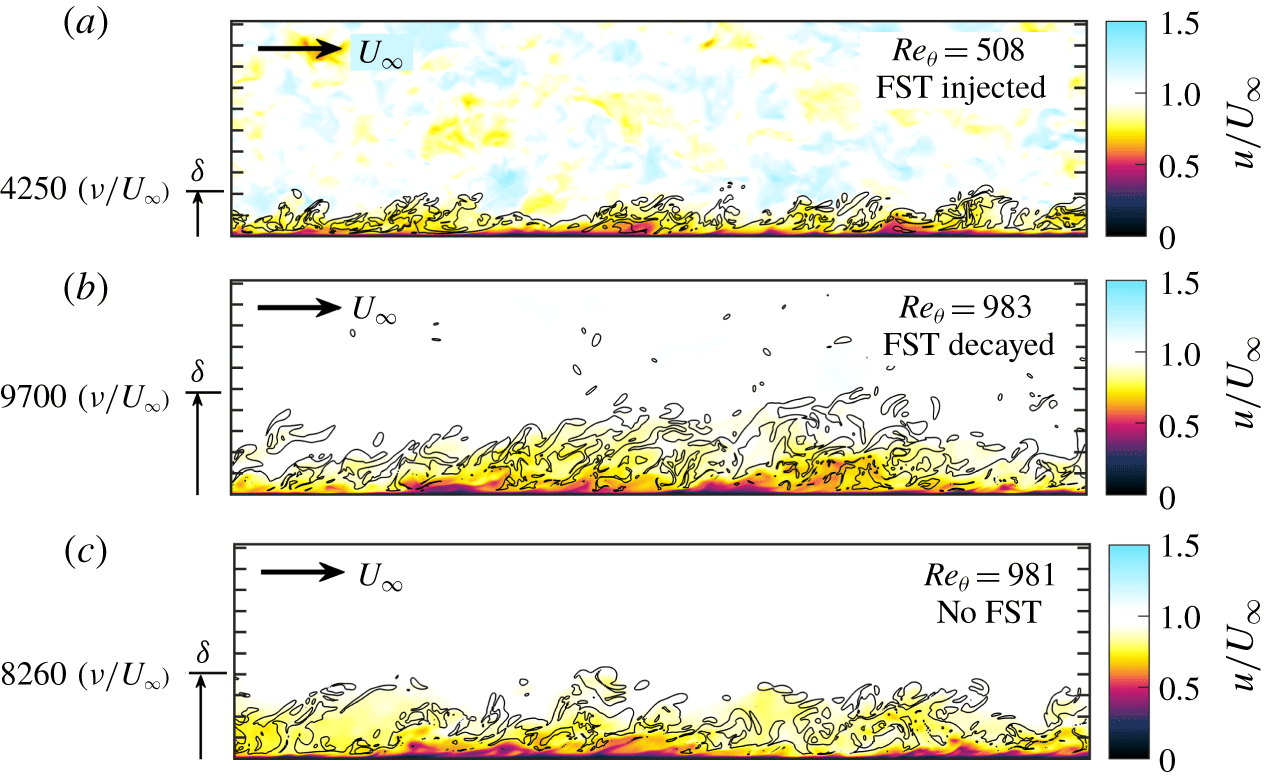
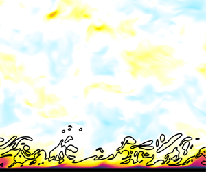
Figure 6 shows a visualisation of boundary layers developing under both quiescent and turbulent free streams comparing experimental images from Hancock & Bradshaw (Reference Hancock and Bradshaw1989) to those from our simulations. The numerical images bear some striking similarities to those of the experiment. For all panels,  $Re_{\unicode[STIX]{x1D703}}\approx 700$. At left are the experimental images, where figure 6(a) is of a boundary layer developing in a quiescent free stream and figure 6(c) is of a boundary layer under mild FST. At right are comparable images of the scalar for the numerical cases. Figure 6(b) is for a quiescent free-stream case (Kozul et al. Reference Kozul, Chung and Monty2016) and figure 6(d) is for the present FST case D. The large-eddy length scale ratio is matched between the experimental and numerical FST cases at $L_{e}^{u}/\unicode[STIX]{x1D6FF}=0.4$, and the intensity differs marginally, being $u_{e}^{\prime }/U_{\infty }=0.03$ for the experimental case with free-stream velocity $U_{\infty }$ and $u_{e}^{\prime }/U_{\infty }=0.04$ for the present case D. It is immediately obvious that the boundary layer with FST is much thicker at the same $Re_{\unicode[STIX]{x1D703}}$ in both the experimental and numerical images. In the quiescent case, we see rounded lobes at the edge of the more compact boundary layer, yet in the bottom images with FST, the edge of the boundary layer is far more jagged, emphasised with the thick white contour at 1 % of the scalar contrast. It is clear from these images that one of the main actions of the FST is to, given the same momentum deficit, increase the spread of the boundary layer by transporting fluid mass away from the wall. This conclusion cannot be reached if vorticity or turbulent kinetic energy is used instead of the scalar (§ 3.2) to demarcate wall-generated turbulence from FST. Note the more subtle increase in the boundary layer thickness $\unicode[STIX]{x1D6FF}$ between figures 6(b) and 6(d). The scalar here demonstrates the significant redistribution of boundary layer fluid, including large excursions of the order of $2\,\unicode[STIX]{x1D6FF}$. Such enhanced excursions due to FST may be particularly relevant in the context of a reacting flow or pollutant originating in the boundary layer.
4.2 Progress of simulations
Figure 7(a) places our simulations amongst several previous experimental studies by plotting the evolution of the relative large-eddy length scale  $L_{e}^{u}/\unicode[STIX]{x1D6FF}$ against the relative velocity scale $u_{e}^{\prime }/U_{\unicode[STIX]{x1D70F}}$. The current cases begin at the top right of each curve and track downward and to the left in time as do those of Hancock & Bradshaw (Reference Hancock and Bradshaw1983) as their measurement location moves downstream in the wind tunnel. The curve for case A (initial simulation fields are HIT with no ‘pre-grown’ boundary layer) is only plotted from $Re_{\unicode[STIX]{x1D703}}\approx 500$ onwards such that the growing boundary layer is behaving canonically following a numerical trip at $Re_{D}=500$ (Kozul et al. Reference Kozul, Chung and Monty2016). Here we are able compare companion cases A and A1. There is some discrepancy in their respective curves in figure 7(a) indicating the history effect. Even when we matched the ‘downstream’ condition at $Re_{\unicode[STIX]{x1D703}}=508$, the difference in their curves indicates an integrated effect upon the boundary layer of case A since it was exposed to FST from the boundary layer’s inception. As a comparison to the dissipation-based scale $L_{e}^{u}$, the evolution of the longitudinal integral length scale $L_{uu,e}$ (2.3) is shown as a function of the relative velocity scale $u_{e}^{\prime }/U_{\unicode[STIX]{x1D70F}}$ in figure 7(b). The value of this length scale is clearly smaller than that of $L_{e}^{u}$, especially at times just after the FST injection. However, a similar relative behaviour of the length scales is demonstrated for the different cases when this integral length scale is used. The unevenness of $L_{uu,e}/\unicode[STIX]{x1D6FF}$ towards the end of the simulation (low $u_{e}^{\prime }/U_{\unicode[STIX]{x1D70F}}$) for cases D and E is a result of the limited domain size where it is likely less reliable.
Flow visualisations. (a,c) Reproduction of figure 9 from Hancock & Bradshaw (Reference Hancock and Bradshaw1989) at  $Re_{\unicode[STIX]{x1D703}}\approx 700$ ( $\unicode[STIX]{x1D6FF}$ extracted from reproductions of these same images in figure 4.14 of Hancock (Reference Hancock1980), these versions preferred for their higher quality): (a) $u_{e}^{\prime }/U_{\infty }\approx 0.0$; (c) $u_{e}^{\prime }/U_{\infty }\approx 0.03$, $L_{e}^{u}/\unicode[STIX]{x1D6FF}_{995}\approx 0.4$. (b,d) Scalar from temporal boundary layer simulations at $Re_{\unicode[STIX]{x1D703}}\approx 700$, $t\approx 1.5\,T_{e,0}$ post-FST injection: (b) with a quiescent free stream from Kozul et al. (Reference Kozul, Chung and Monty2016); (d) present case D with FST, $u_{e}^{\prime }/U_{\infty }\approx 0.04$, $L_{e}^{u}/\unicode[STIX]{x1D6FF}\approx 0.4$. White contours in (b,d) show location of 1 % scalar concentration; thick grey contour in (d) estimates the distance $\ell _{\mathscr{D}}$ over which the scalar diffuses from the time of FST injection to the time shown here (cf. § 4.6). Assuming the same aspect ratio in (a,c), the streamwise extent shown for (b,d) is approximately equivalent in units of $\unicode[STIX]{x1D708}/U_{\infty }$; white tickmarks on the vertical axes of these panels show intervals of $2000\,\unicode[STIX]{x1D708}/U_{\infty }$.
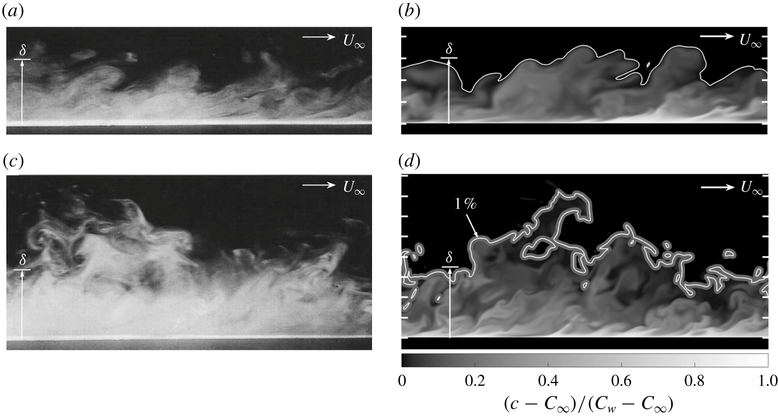
Regime diagram showing cases (coloured curves as per table 2) for two different definitions of the large-eddy length scale on the vertical axis. (a) Dissipation-based scale  $L_{e}^{u}$ from (2.4); (b) longitudinal integral length scale $L_{uu,e}$ (2.3) within the free stream: ●, Hancock & Bradshaw (Reference Hancock and Bradshaw1983); $\times$, Dogan et al. (Reference Dogan, Hanson and Ganapathisubramani2016). Curves track downward towards the left-bottom corner.
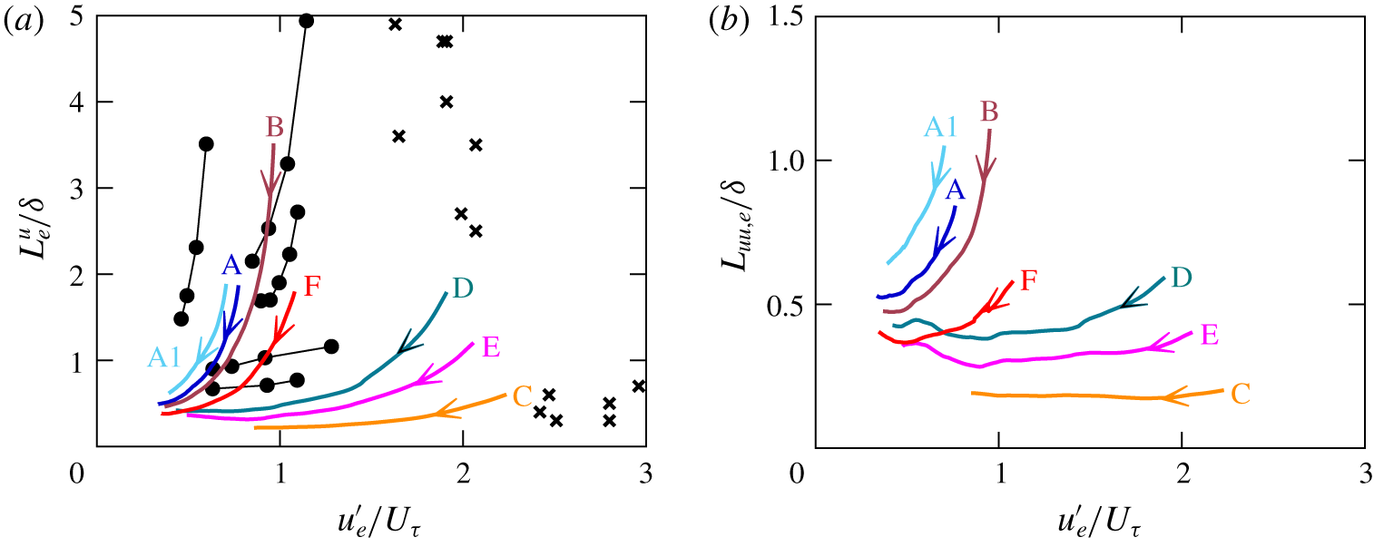
Figure 8(a) shows that the boundary layer thickness  $\unicode[STIX]{x1D6FF}$ increases in time over that for a boundary layer under a quiescent free stream for cases A1, B, D, E and F. The increase shown is compared to the boundary layer thickness at the time step prior to FST injection $\unicode[STIX]{x1D6FF}_{0}$. Dashed lines show the continued development of the boundary layer thickness, coloured by each case, when the FST is not injected. For cases A1 and B, this is the same precursor boundary layer simulation that was prolonged, these cases only differing in the HIT that was injected, and therefore the $T_{e,0}$ by which the horizontal axis is scaled. Case A, where the FST formed the initial velocity fields, is excluded here (and from figures 8b and 8c) since for that case $\unicode[STIX]{x1D6FF}_{0}$ is the non-physical numerical trip making such a comparison physically meaningless. Also in case A the boundary layer is transitioning at early times, where the focus here is on the impact of FST on the fully turbulent boundary layer. Only a limited development extent could be viewed for case C, where the simulation was halted at the point shown, since $\unicode[STIX]{x1D6FF}$ reached our imposed simulation limit of $1/3$ of the box height $L_{z}$, at which point $\unicode[STIX]{x1D6FF}\equiv \unicode[STIX]{x1D6FF}_{99}$ becomes unreliable. Figure 8(b) shows that the development of momentum thickness $\unicode[STIX]{x1D703}$ is more or less unaffected by the FST for all cases.
(a) Development of  $\unicode[STIX]{x1D6FF}/\unicode[STIX]{x1D6FF}_{0}$ with time post-FST injection for all present cases except case A, curves coloured as per table 2: – – –, similar for precursor ‘pre-grown’ boundary layers allowed to continue development without FST; $\unicode[STIX]{x1D6FF}_{0}$ is the boundary layer thickness at the time step prior to FST injection. (b) Development of $\unicode[STIX]{x1D703}/\unicode[STIX]{x1D703}_{0}$ with time post-FST injection; $\unicode[STIX]{x1D703}_{0}$ is the momentum thickness at the time step prior to FST injection. (c) Development of $U_{\unicode[STIX]{x1D70F}}/U_{\unicode[STIX]{x1D70F},0}$ with time post-FST injection; $U_{\unicode[STIX]{x1D70F},0}$ is the friction velocity at the time step prior to FST injection. Note that the ‘pre-grown’ boundary layers are the same for cases A1 and B, yet the FST was allowed to decay sometime before injection to form case A1, meaning $T_{e,0}$ differs. (d) Boundary layer spreading rate as a function of time post-FST injection for all present cases except case C: – – –, spreading rate for precursor ‘pre-grown’ boundary layers allowed to continue development without FST; ●, point at which each interaction has become ‘weak’, i.e. where spreading rate tempers to the quiescent value. Data for (d) are window-averaged over time intervals of ${\approx}0.03\,T_{e,0}$.

Figure 8(c) shows that FST increases  $U_{\unicode[STIX]{x1D70F}}$ over that for the quiescent boundary layer for cases A1, B, D and F. Here the largest change is found for case D compared to the boundary layer allowed to continue growing under a quiescent free stream (dashed line), with smaller divergences from the quiescent curves for cases A1, B and F. Interestingly, case E, which displayed a significant increase in $\unicode[STIX]{x1D6FF}$ over the quiescent development value in figure 8(a), does not show a sustained gain in $U_{\unicode[STIX]{x1D70F}}$. Therefore for this case at least, the FST is mostly an outer-scale interaction working only to increase the boundary layer thickness. Generally, any increases in $U_{\unicode[STIX]{x1D70F}}$ appear to be more short-lived: for case D the FST curve appears on its way to merge with the quiescent curve by ${\approx}3\,t/T_{e,0}$ measured post-FST injection. The same cannot be said for the seemingly more permanently increased $\unicode[STIX]{x1D6FF}$ in figure 8(a). The gain in friction Reynolds number due to the FST can be directly calculated at any $t/T_{e,0}$ following FST injection from figure 8(a,c) using $[(Re_{\unicode[STIX]{x1D70F}})_{FST\,case}-(Re_{\unicode[STIX]{x1D70F}})_{Q}]/Re_{\unicode[STIX]{x1D70F},0}=[(U_{\unicode[STIX]{x1D70F}}/U_{\unicode[STIX]{x1D70F},0})(\unicode[STIX]{x1D6FF}/\unicode[STIX]{x1D6FF}_{0})]_{FST\,case}-[(U_{\unicode[STIX]{x1D70F}}/U_{\unicode[STIX]{x1D70F},0})(\unicode[STIX]{x1D6FF}/\unicode[STIX]{x1D6FF}_{0})]_{Q}$, where $Q$ is for quiescent. Any such increase due to FST injection will be proportionally more attributable to an increase in $\unicode[STIX]{x1D6FF}$ rather than an increase in $U_{\unicode[STIX]{x1D70F}}$ (the vertical scale of figure 8a showing $\unicode[STIX]{x1D6FF}/\unicode[STIX]{x1D6FF}_{0}-1$ is ten times that of figure 8c showing $U_{\unicode[STIX]{x1D70F}}/U_{\unicode[STIX]{x1D70F},0}-1$).
Figure 8(d) plots the boundary layer spreading rate  $U_{\infty }^{+}(\text{d}\unicode[STIX]{x1D6FF}/\text{d}X)$ similarly as a function of time post-FST injection. For cases D and E we see large, short-lived spikes in the spreading rate above that for the boundary layer allowed to continue growing under a quiescent free stream. Case D with the smaller $e_{0}=T_{\unicode[STIX]{x1D6FF},0}/T_{e,0}=1.2$ seems to react faster and exhibit a larger spreading rate than case E with $e_{0}=1.9$. From figure 8(a,c), we know the increased spreading rate for case E is due mostly to the increase in the rate of growth of $\unicode[STIX]{x1D6FF}$ in a more purely outer-flow interaction. Case F displays a more modest but still significant increase in the spreading rate at early times, especially at ${\approx}0.5\,t/T_{e,0}$. The effect is much weaker for the other low-intensity cases A, A1 and B although a small increase is seen for case B over its corresponding quiescent case. The early elevated spreading rates of cases B, D and E relax back towards quiescent values as the FST decays in time and these approximate points are indicated with filled circles. For temporal wakes embedded into HIT, Rind & Castro (Reference Rind and Castro2012) similarly found an increase in the growth rate of the wake half-width, with a stronger effect for a higher external turbulence intensity. The spreading rate for case C is not shown in figure 8(d) since it appeared unreliable.
The gain in the skin friction coefficient due to FST injection compared to the canonical values of the quiescent boundary layer ( $(C_{f})_{FST\,case}-(C_{f})_{Q}=\unicode[STIX]{x0394}C_{f}>0$ for $C_{f}=2\,(U_{\unicode[STIX]{x1D70F}}/U_{\infty })^{2}$) is shown in figure 9, and is considerably larger when computed at matched $Re_{\unicode[STIX]{x1D70F}}$ than that at matched $Re_{\unicode[STIX]{x1D703}}$. Increases in the skin friction coefficient due to FST have been reported previously (Hancock & Bradshaw Reference Hancock and Bradshaw1983), as have increases in the mass transfer coefficient or Stanton number $St$ (Blair Reference Blair1983a). This gain is directly proportional to the gain $U_{\unicode[STIX]{x1D70F}}/U_{\unicode[STIX]{x1D70F},0}$ shown in time post-FST injection in figure 8(c). Figure 8(a) shows the often significant change in $\unicode[STIX]{x1D6FF}$ for the different cases, meaning values along both axes are potentially altered in figure 9(a) in the case of boundary layers developing under FST. Since $(C_{f})_{Q}$ decreases with increasing friction Reynolds number $Re_{\unicode[STIX]{x1D70F}}=U_{\unicode[STIX]{x1D70F}}\unicode[STIX]{x1D6FF}/\unicode[STIX]{x1D708}$, increasing $Re_{\unicode[STIX]{x1D70F}}$ via an increase in $\unicode[STIX]{x1D6FF}$, but not $U_{\unicode[STIX]{x1D70F}}$, will nonetheless give $\unicode[STIX]{x0394}C_{f}>0$ with no change in $(C_{f})_{FST\,case}=2\,(U_{\unicode[STIX]{x1D70F}}/U_{\infty })_{FST\,case}^{2}$. Thus the development of $C_{f}$ with respect to $Re_{\unicode[STIX]{x1D70F}}$ may be altered via an ‘artificial’ increase in $Re_{\unicode[STIX]{x1D70F}}$, rather than a genuine change in the wall-defined value of $C_{f}$ due to, say, the penetration of free-stream fluid. That is, a gain in $C_{f}$ over that for the canonical quiescent boundary layer will be due at least in part to the enhanced growth rate of the boundary layer thickness $\unicode[STIX]{x1D6FF}$ at fixed $\unicode[STIX]{x0394}Re_{X=U_{\infty }t}=Re_{\unicode[STIX]{x0394}X=U_{\infty }\unicode[STIX]{x0394}t}$ (i.e. at a fixed time) post-HIT injection when compared to the quiescent case. The development of momentum thickness $\unicode[STIX]{x1D703}$ post-FST injection is much less affected than that of $\unicode[STIX]{x1D6FF}$ (figure 8a,b) and therefore $(\unicode[STIX]{x0394}C_{f})_{=Re_{\unicode[STIX]{x1D703}}}$ (figure 9b, at matched $Re_{\unicode[STIX]{x1D703}}$) will be almost solely due to a change in $U_{\unicode[STIX]{x1D70F}}$, if indeed there is one. Gain $(\unicode[STIX]{x0394}C_{f})_{=Re_{\unicode[STIX]{x1D70F}}}$ (figure 9a, at matched $Re_{\unicode[STIX]{x1D70F}}$) is larger due to the permanent shift in $\unicode[STIX]{x1D6FF}$, irrespective of changes in $U_{\unicode[STIX]{x1D70F}}$. Case E, for example, shows a considerable and persistent increase in $\unicode[STIX]{x1D6FF}$ post-FST injection compared to the quiescent case, although no durable increase in $U_{\unicode[STIX]{x1D70F}}$. As a result, the peak $\unicode[STIX]{x0394}C_{f}$ for this case appears more than twice as large when plotting at matched $Re_{\unicode[STIX]{x1D70F}}$ to the quiescent boundary layer (figure 9a) than at matched $Re_{\unicode[STIX]{x1D703}}$ (figure 9b). Case E is therefore particularly illustrative: it is important to correctly attribute the origin of an apparent gain $\unicode[STIX]{x0394}C_{f}$ for boundary layers developing under FST. The present temporal technique permits appraisal of these separate modifications to the boundary layer by the FST.
Furthermore, we point out the almost horizontal (albeit noisy) gain in the skin friction coefficient in figure 9 for case A, which had the HIT as the initial fields when the boundary layer simulation began, in contrast to all other cases where the FST was injected over a ‘pre-grown’ boundary layer. Where  $\unicode[STIX]{x0394}C_{f}$ for the other cases tends to rise as the effect of the FST is felt by the boundary layer (i.e. via an increased growth in $\unicode[STIX]{x1D6FF}$ and decrease in $U_{\unicode[STIX]{x1D70F}}$), before decreasing at a later time (higher Reynolds number), the skin friction coefficient gain for case A appears approximately constant. Corresponding with this more ‘passive’ behaviour, case A shows no increased spreading rate in figure 8(d) for the same simulation period as shown in figure 9. The change in FST intensity and length scales for case A is very similar to its companion case A1 for the development extent shown in figure 9, yet $\unicode[STIX]{x0394}C_{f}$ shows a sharper increase for case A1 (although a lower peak $\unicode[STIX]{x0394}C_{f}$) as the boundary layer responds to the FST. Case A’s behaviour here points to an upstream perturbation to the burgeoning boundary layer, from which full recovery back to quiescent boundary layer values (i.e. $\unicode[STIX]{x0394}C_{f}=0$) remains elusive.
Gain in the skin friction coefficient due to FST injection with respect to the quiescent boundary layer of Kozul et al. (Reference Kozul, Chung and Monty2016): (a) at matched  $Re_{\unicode[STIX]{x1D70F}}$; (b) at matched $Re_{\unicode[STIX]{x1D703}}$. The curve for case A (initial simulation fields are HIT with no ‘pre-grown’ boundary layer) is plotted from $Re_{\unicode[STIX]{x1D703}}\approx 500$.
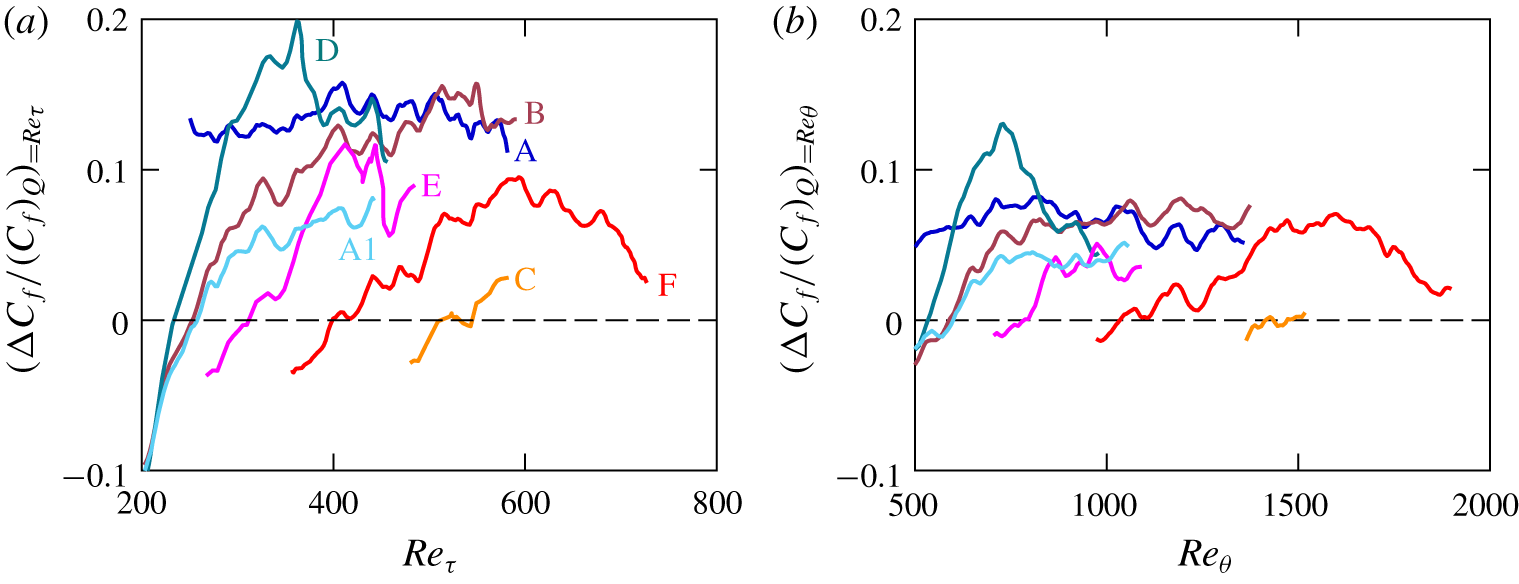
4.3 Comparisons of velocity statistics to experimental data
Notwithstanding a non-physical adjustment period after the artificial combination of fields, we are able to find some agreement with an experimental study of the same problem (Nagata et al. Reference Nagata, Sakai and Komori2011) for case D in figure 10, showing subdued mean streamwise velocity and  $w_{rms}^{+}$ profiles. The small-scale turbulence of Nagata et al. (Reference Nagata, Sakai and Komori2011) allows for quantitative comparison to the present cases, although the upstream history is different compared to our synthesised fields. Here $Re_{\unicode[STIX]{x1D70F}}$ and $u_{e}^{\prime }/U_{\unicode[STIX]{x1D70F}}$ are roughly matched for the two cases, although the length scale ratio $L_{e}^{u}/\unicode[STIX]{x1D6FF}$ is larger for the case of Nagata et al. (Reference Nagata, Sakai and Komori2011) being $0.403$, compared to $0.235$ for the present case D at this point in the simulation. An important FST effect is the reduction of the boundary layer wake (referring to the region external to the logarithmic region) in the mean streamwise profile in figure 10(a): Blair (Reference Blair1983b) reported a totally subdued wake for a value of around $u_{e}^{\prime }/U_{\infty }\approx 0.05$. For this level of turbulence at $u_{e}^{\prime }/U_{\unicode[STIX]{x1D70F}}=0.50,u_{e}^{\prime }/U_{\infty }\approx 0.02$, we find the wake weakened yet still present. The diminishing wake is a manifestation of diminishing intermittency in the outer region of the boundary layer due to the free-stream disturbances. The profile of $u_{rms}^{+}$ (not shown) is identical to the quiescent case at matched $Re_{\unicode[STIX]{x1D70F}}$ from the wall up to $z^{+}\approx 400$. Note the flat $w_{rms}^{+}$ profile in figure 10(b) away from the wall: being well outside the boundary layer, this is where the flow resembles HIT. Figure 10(c,d) shows a subdued Reynolds shear stress profile plotted against both inner and outer coordinates. The present DNS demonstrates the negligible effect on the Reynolds shear stress due to FST very close to the wall for $z^{+}\lesssim 10$ in figure 10(c). The substantial depression of the Reynolds shear stress profile for $z^{+}\gtrsim 10$ with respect to the quiescent case seems wholly attributable to the diminished $w_{rms}^{+}$ profile since a decrease with respect to the quiescent case is evident across the same region in figure 10(b). Figure 10(d) with a linear horizontal axis gives a more tangible view of the effect of the FST with respect to the large-eddy scale of the boundary layer $\unicode[STIX]{x1D6FF}$.
FST-altered profiles for case D at  $Re_{\unicode[STIX]{x1D70F}}\approx 450$ ( $Re_{\unicode[STIX]{x1D703}}\approx 940$): (a) mean streamwise velocity; (b) root-mean-squared wall-normal velocity fluctuations. Reynolds shear stress profiles plotted against (c) inner-scaled wall-normal distance and (d) outer-scaled distance: —— (teal), present case D, at $t/T_{e,0}\approx 3.4$ post-FST injection, with FST parameters $L_{e}^{u}/\unicode[STIX]{x1D6FF}=0.403$, $u_{e}^{\prime }/U_{\unicode[STIX]{x1D70F}}=0.43$;
——, quiescent temporal boundary layer from Kozul et al. (Reference Kozul, Chung and Monty2016) at matched
$u_{e}^{\prime }/U_{\unicode[STIX]{x1D70F}}=0.43$;
——, quiescent temporal boundary layer from Kozul et al. (Reference Kozul, Chung and Monty2016) at matched  $Re_{\unicode[STIX]{x1D70F}}\approx 450$ ( $Re_{\unicode[STIX]{x1D703}}\approx 1200$);
  , quiescent spatial boundary layer of Simens et al. (Reference Simens, Jiménez, Hoyas and Mizuno2009) at $Re_{\unicode[STIX]{x1D70F}}=445$ ( $Re_{\unicode[STIX]{x1D703}}=1100$); ▲, experimental case LG-2 of Nagata et al. (Reference Nagata, Sakai and Komori2011) at $Re_{\unicode[STIX]{x1D70F}}=475$ ( $Re_{\unicode[STIX]{x1D703}}=1100$) with FST parameters $L_{e}^{u}/\unicode[STIX]{x1D6FF}=0.235$, $u_{e}^{\prime }/U_{\unicode[STIX]{x1D70F}}=0.45$.
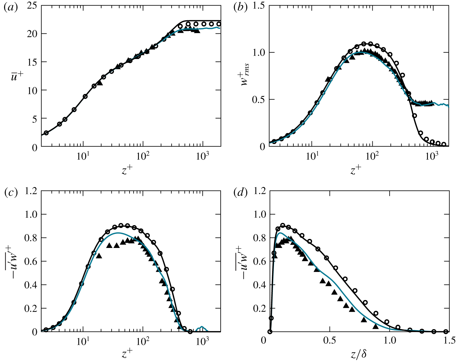
Although we would not necessarily expect to find agreement with this experimental boundary layer, which has been exposed to FST from inception in contrast to ours, for our case D the FST has indeed effected change deep into the boundary layer. Our injected FST apparently affects our boundary layer in a similar way to that in this particular experimental case. We consider this an example of a ‘strong’ boundary layer–FST interaction. In contrast to these modified profiles for case D, similar profiles for case C showed no discernible change from the quiescent profiles due to the presence of the FST. We highlight the large difference in  $T_{\unicode[STIX]{x1D6FF},0}/T_{e,0}$ between cases C and D, which may explain why the boundary layer in case C appears to ignore the FST in an apparent ‘weak’ interaction with it.
4.4 Intermittency factor
The intermittency factor  $\unicode[STIX]{x1D6FE}$ is shown in figure 11. We find that the effect of the FST is to spread the boundary layer edge significantly compared with the boundary layer under a quiescent free stream for all cases. The intermittency profile is here calculated as the fraction of points in a homogeneous $xy$ plane above 1 % of the scalar contrast $C_{w}-C_{\infty }$. Figure 11(a) corresponds to the time of FST injection, figure 11(b) after $t\approx 0.9\,T_{e,0}$ and figure 11(c) after $t\approx 1.7\,T_{e,0}$. That is, curves are plotted at roughly the same time intervals in terms of the initial FST large-eddy time scale for all cases. This definition of the intermittency is directly inspired by the approach of Hancock & Bradshaw (Reference Hancock and Bradshaw1989), where $\unicode[STIX]{x1D6FE}$ was defined as the fraction of total time at a measurement location for which the flow in their wind tunnel was ‘hot’ (based primarily on the detection of an increase in the measured temperature to a specified level above the background ‘cold’ level) in their heated boundary layer. This is a more quantitative representation of the smeared-out boundary layers shown in figure 6. Drawing attention to two cases in particular, we note the initial FST intensity $u_{e,0}^{\prime }/U_{\unicode[STIX]{x1D70F},0}$ is similar for cases C and D. Scaling with $\unicode[STIX]{x1D6FF}$ along the horizontal axis eases the comparison between these and other cases: the value of $\unicode[STIX]{x1D6FF}$ at the time of FST injection differs by a factor of almost 3 between cases C and D for example. For all cases except case C, there is a flattening of the $\unicode[STIX]{x1D6FE}$ profile at the later times at $z/\unicode[STIX]{x1D6FF}\approx 1.5$, this effect being most marked for case D. The effect is weakest for case C, which has a high initial relative large-eddy turnover time scale $e_{0}=T_{\unicode[STIX]{x1D6FF},0}/T_{e,0}$; curves for case C in figure 11(b,c) appear offset from that of the quiescent boundary layer rather than smeared out. The curve for case D in figure 11(b) sits noticeably higher than that for case C over the region $1\lesssim z/\unicode[STIX]{x1D6FF}\lesssim 2$. Thus the smearing effect appears to be strongest for case D, which has a lower $e_{0}$ than case C, and persists for the longest time (i.e. most flattened in figure 11c).
Intermittency factor calculated as the fraction of points at each homogeneous  $xy$ plane where the scalar exceeds 1 % of the scalar contrast $C_{w}-C_{\infty }$: (a) at the time of FST injection (not relevant for case A); (b) at $t\approx 0.9\,T_{e,0}$ post-FST injection; (c) at $t\approx 1.7\,T_{e,0}$ post-FST injection. Quiescent temporal boundary layer from Kozul et al. (Reference Kozul, Chung and Monty2016) at matched $Re_{\unicode[STIX]{x1D703}}$ to
  , case C in each panel; and – – –, case D in each panel, together spanning the range of $Re_{\unicode[STIX]{x1D703}}$ covered by the current simulations. Coloured curves as per table 2.
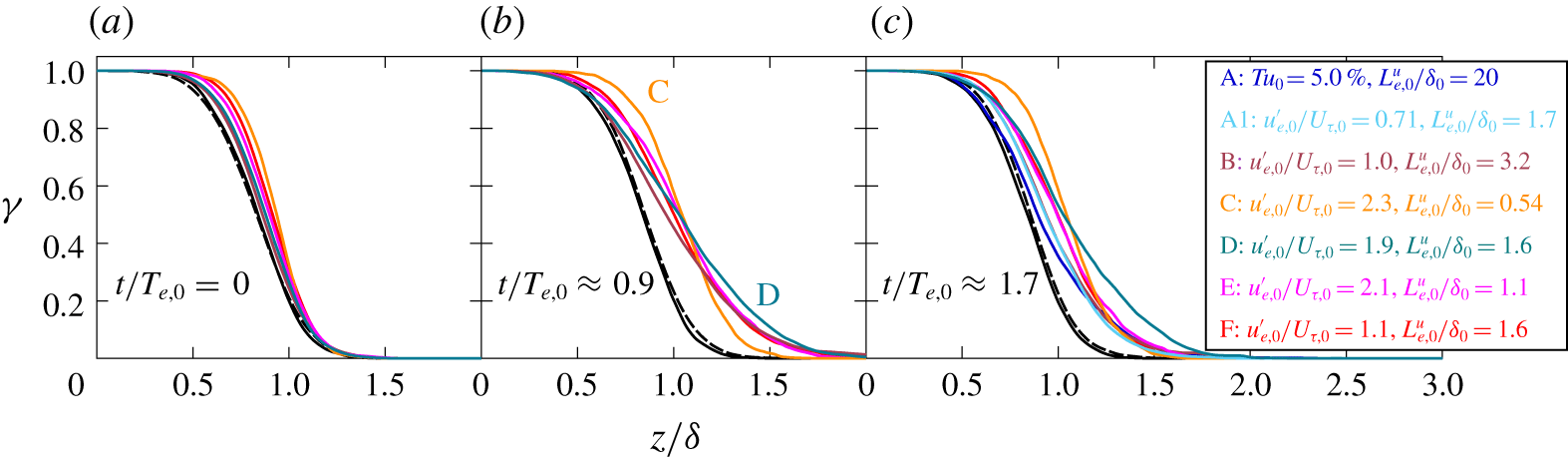
Wall-normal velocity variance evolution in time for all present cases from table 2; curves darken as time (measured post-FST injection) progresses as indicated by the arrows. Top row shows cases with lower-intensity FST at injection with (a) case A,  $u_{e,0}^{\prime }/U_{\infty }=5.0$; (b) case A1, $u_{e,0}^{\prime }/U_{\infty }=3.6$; and (c) case B, $u_{e,0}^{\prime }/U_{\infty }=5.0$. Bottom row for high-intensity cases, all with $u_{e,0}^{\prime }/U_{\infty }=10$: (d) case D; (e) case E; and (f) case C. Curves in grey for temporal boundary layer developing under a quiescent free stream from Kozul et al. (Reference Kozul, Chung and Monty2016), with matched Reynolds number to the final curve shown in each panel: – – – (grey), at matched $Re_{\unicode[STIX]{x1D703}}$; —— (grey), at matched $Re_{\unicode[STIX]{x1D70F}}$. Inset in each panel shows the peak $w_{rms}^{+}$ value (for $z^{+}<100$) for each of the times $t/T_{e,0}$ post-FST injection shown, and compares it to that for the reference quiescent boundary layer (indicated by ‘Ref.’) at matched $Re_{\unicode[STIX]{x1D703}}$. In (b): – - – -, case A at $t/T_{e,0}=2$ for comparison.
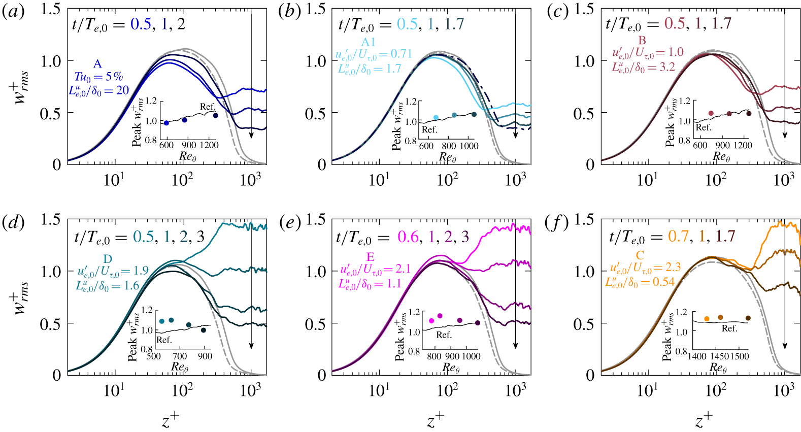
4.5 Wall-normal velocity variance profiles in time
In figure 10, the profiles for case D are plotted at a single Reynolds number to best match that of the experimental case to which it is being compared. In our temporally developing flow, this corresponds to one point in time following (‘downstream of’) the FST injection. A major strength of the present technique is the possibility of viewing the entire boundary layer–FST interaction as it unfolds.
Figure 12 plots the profiles at multiple points in time for all the present cases showing different responses to the injected FST. Figure 12(a–c) shows the three cases with lower FST intensity at injection (cases A, A1 and B) and figure 12(d–f) shows those at higher FST intensity (cases D, E and C). Curves in grey show profiles for the quiescent boundary layer of Kozul et al. (Reference Kozul, Chung and Monty2016) matched to the  $Re_{\unicode[STIX]{x1D703}}$ and $Re_{\unicode[STIX]{x1D70F}}$ of the final curves in each panel. Insets in each panel show the evolution of the peak $w_{rms}^{+}$ (for $z^{+}<100$) at the same $t/T_{e,0}$ for which profiles are plotted and compares them to that for the quiescent boundary layer at matched $Re_{\unicode[STIX]{x1D703}}$ (since figure 8 showed that the development of $\unicode[STIX]{x1D6FF}$, which will alter the development of $Re_{\unicode[STIX]{x1D70F}}$, was much more affected than $\unicode[STIX]{x1D703}$). For example, the second coloured circle marker on all insets in this figure shows the peak $w_{rms}^{+}$ at $t/T_{e,0}=1$ post-FST injection compared with that of the quiescent boundary layer at matched $Re_{\unicode[STIX]{x1D703}}$.
In figure 12(a–c) (lower FST intensity), small decreases from the quiescent profiles at the final times are evident. Indeed, only very subtle differences in the peak  $w_{rms}^{+}$ are evident during the length of the simulations (see insets). Ingested FST fluid nonetheless lowers the final peak $w_{rms}^{+}$ slightly for cases A and B. Differences with respect to the quiescent case are smallest for case A1, where the injected FST is the partially decayed field used for cases A and B. The curve at $t/T_{e,0}$ for case A was added to figure 12(b) for comparison to its companion case A1 at $t/T_{e,0}=1.7$. The curves are not exactly the same, indicating the history affect, yet this comparison (along with the agreement of case D with experimental data in figure 10) demonstrates the present technique’s ability to give ‘physical’ downstream fields. In figure 12(d–f), the three cases have the same $Tu\equiv u_{e}^{\prime }/U_{\infty }$ (and similar $u_{e}^{\prime }/U_{\unicode[STIX]{x1D70F}}$) when the FST is injected, yet their relative length scales differ significantly: at injection $L_{e}^{u}/\unicode[STIX]{x1D6FF}\approx 1.6$ for case D, ${\approx}1.1$ for case E and ${\approx}0.54$ for case C. We find that despite being exposed to the same levels of FST intensity, the outcome is different for the high-intensity cases, with the FST in case D able to, after some time, effect change in the $w_{rms}^{+}$ profile with respect to a quiescent spatial DNS profile at a matched $Re_{\unicode[STIX]{x1D70F}}$ (subdued peak for $z^{+}\gtrsim 40$ after $t\approx 3\,T_{e,0}$ in figure 12d). Only a mild difference from the quiescent case is found in the curve at the final $t/T_{e,0}=3$ shown for case E (figure 12e); however, the evolution of the peak $w_{rms}^{+}$ is similar to that of case D, showing an early increase with respect to the reference quiescent case followed by a decline as the FST decays. We suggest the observed lowering of the final peak $w_{rms}^{+}$ as compared to the reference quiescent cases is due to the intensity of the FST being lower than the quiescent peaks at this point. At early times when the FST is stronger, the peaks for cases B, D and E in particular appear higher than that for the quiescent boundary layer, reflecting an early FST intensity level that exceeds the peak $w_{rms}^{+}$ of the reference quiescent boundary layer.
There is a key difference between cases D and E: at  $t/T_{e,0}=3$, we suggest that there have been more substantial FST fluid incursions deep into the boundary layer in case D than in case E, resulting in a lowering of the final peak value. The final circle marker in the inset of figure 12(d) for case D lies below that for the quiescent boundary layer, whereas the final circle marker for case E in figure 12(e) lies directly on the black curve, meaning the peak $w_{rms}^{+}$ is unaltered due to the FST at this later time. This will be further explored in § 4.6. A similar conclusion (i.e. final peak $w_{rms}^{+}$ lower than that for the reference quiescent case) is demonstrated by the low-intensity cases in figure 12(a–c); however, the effect is more subtle since the starting FST is weaker. A conclusion on case C is precluded by the limited timespan available; however, we note that changes in the profiles of other cases were effected after similar time delays of $t\approx 1.7\,T_{e,0}$. In figure 12, time intervals of $t/T_{e,0}$ are equivalent for the evolution of HIT in all cases except A1, whose free stream was seeded with a partially decayed HIT field possessing a different $T_{e,0}$ (table 1). Yet, time passed in terms of the initial boundary layer large-eddy time scale $T_{\unicode[STIX]{x1D6FF},0}$ is very different across the different cases, by a factor equivalent to the difference in $e_{0}=T_{\unicode[STIX]{x1D6FF},0}/T_{e,0}$ shown in table 2. Thus the boundary layer time scale for case C is roughly three times that for case D, and we suggest that this parameter effectively dictates the ‘reaction’ time of the boundary layer to the FST.
Figure 12 suggests that the boundary layer–FST interaction in our cases can be largely understood as a simple mixing of the two flows. The peaks in the  $w_{rms}^{+}$ profiles (insets) are increased when the FST is higher than the peak of the wall-generated turbulence, and then decreased when the FST is lower than that of the wall-generated turbulence. Section 4.6 offers conditional statistics building on this basic idea. For wakes subject to external turbulence, Pal & Sarkar (Reference Pal and Sarkar2015) introduced an argument based on $u_{e}^{\prime }/u_{cl}^{\prime }$, where $u_{cl}^{\prime }$ is the wake turbulence at the centreline, and found this to be the key parameter governing the influence of external fluctuations, and not $u_{e}^{\prime }/U_{0}$, where $U_{0}$ is the centreline deficit velocity. In the present wall-bounded flow we can take $u_{cl}^{\prime }$ to be analogous to the peak in velocity variance profiles (i.e. $w_{rms,peak}^{\prime }$ in the insets of figure 12). We indeed see the influence of the relative ratio of $w_{e}^{\prime }/w_{rms,peak}^{\prime }$ as stated above. Pal & Sarkar (Reference Pal and Sarkar2015) reported that the external turbulence and centreline turbulence tend to eventually decay at similar rates. This is in contrast to the boundary layer where the inner peak is ever energised by $U_{\unicode[STIX]{x1D70F}}$, and thus the ratio $w_{e}^{\prime }/w_{rms,peak}^{\prime }$ always falls as the FST decays. Whether the boundary layer is impacted by the FST while $w_{e}^{\prime }/w_{rms,peak}^{\prime }$ is still above unity (Pal & Sarkar Reference Pal and Sarkar2015) is governed by the relative large-eddy turnover time scale. This effectively dictates the ‘adjustment time’ required between the boundary layer and FST.
4.6 Free-stream contributions to wall-normal Reynolds stress profiles
Boundary layer and FST contributions to the wall-normal Reynolds stress profiles deduced via conditional averaging on the passive scalar: ——, contribution from the boundary layer; – – –, contribution of FST;  , sum of two profiles, equivalent to non-conditionally averaged profiles. (a,d,g) Case D; (b,e,h) case E; (c,f,i) case C. (a–c) At the time of FST injection; (d–f) at $t\approx 0.9\,T_{e,0}$ after FST injection; (g–i) at $t\approx 1.7\,T_{e,0}$ after FST injection. Curves in grey are for the boundary layer developing under a quiescent free stream from Kozul et al. (Reference Kozul, Chung and Monty2016) at matched $Re_{\unicode[STIX]{x1D70F}}$ for each panel. Note that the vertical scale in (a–c) differs from that of the subsequent panels.
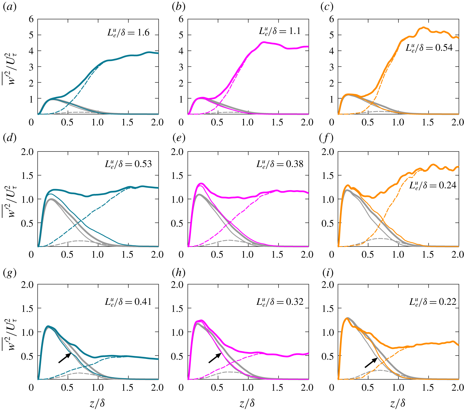
We seek to further dissect the profiles shown in figure 12 for the high-intensity cases. This analysis follows that of Hancock & Bradshaw (Reference Hancock and Bradshaw1989) where the turbulent free-stream fluid was distinguished from that of the wall-generated turbulent flow by heating the boundary layer. In the present case, the passive scalar released at the wall will ‘mark’ that fluid as originating in the boundary layer. Figure 13 shows the ‘free-stream’ versus ‘boundary-layer’ contributions to the wall-normal Reynolds stress profile  $\overline{w^{\prime 2}}/U_{\unicode[STIX]{x1D70F}}^{2}$ for present cases C, D and E. We here use the same thresholding for the conditional averages as used for the injection of the FST as per (3.1): if the scalar concentration is below 5 % of the scalar wall contrast $C_{w}-C_{\infty }$, it will be considered to be a free-stream contribution, else it is deemed to be wall-generated turbulence for the purposes of the present analysis. We note a 1 % threshold was used in the flow visualisation shown in figure 6 and for calculating the intermittency profiles of figure 11. This was both to emphasise differences between the quiescent and FST cases, and since $\unicode[STIX]{x1D6FF}$ is based on the 99 % thickness throughout this work. In contrast a 5 % threshold is more appropriate for figure 13 which directly considers ‘free-stream’ or ‘boundary-layer’ fluid, following the synthesis of these fields via 5 % thresholding. The quiescent boundary layer of Kozul et al. (Reference Kozul, Chung and Monty2016) is subjected to the same analysis and curves are shown at matched $Re_{\unicode[STIX]{x1D70F}}$ in each of the panels for reference. However, it should be noted that our passive scalar is diffusive, with $Sc=\unicode[STIX]{x1D708}/\mathscr{D}=1$, for $\mathscr{D}$ diffusivity of the scalar. At the latest time shown in figure 13, $t\approx 1.7\,T_{e,0}$ following FST injection, the scalar will diffuse over a length $\ell _{\mathscr{D}}\approx \sqrt{2\,\mathscr{D}\,t}=\sqrt{2\,(\unicode[STIX]{x1D708}/Sc)1.7\,T_{e,0}}\approx 1.8\sqrt{T_{e,0}\,U_{\infty }^{2}/\unicode[STIX]{x1D708}}\,(\unicode[STIX]{x1D708}/U_{\infty })\lesssim 500\,\unicode[STIX]{x1D708}/U_{\infty }$ (Westerweel et al. Reference Westerweel, Fukushima, Pedersen and Hunt2009), where $T_{e,0}\,U_{\infty }^{2}/\unicode[STIX]{x1D708}$ is noted in table 2 for all the present cases. This corresponds to a quarter of one of the tickmark intervals shown in figures 5 and 6. As a fraction of the temporal mean of the boundary layer thickness $\overline{\unicode[STIX]{x1D6FF}}$ over $t=[0{-}1.7]\,T_{e,0}$ post-FST injection, $\ell _{\mathscr{D}}\lesssim 7\,\%$ of the smallest $\overline{\unicode[STIX]{x1D6FF}}$ (case D). The error incurred in considering the scalar as a ‘marker’ of the wall-generated turbulence does not impede the analysis, since changes potentially due to diffusion in the curves conditioned on the scalar in figure 13 are small compared to the horizontal extent shown ( $2\,\unicode[STIX]{x1D6FF}$). Moreover, it is small compared to the 50–200 % growth in $\unicode[STIX]{x1D6FF}$ compared to $\unicode[STIX]{x1D6FF}_{0}$ by this time post-FST injection (figure 8a), due in large part to the increasing Reynolds number irrespective of FST.
Figure 13(a–c) shows the penetration depth of the FST to be similar for the three cases at the time of FST injection. The picture changes at a later time. In figure 13(d) for case D and figure 13(e) for case E, after about  $t\approx 0.9\,T_{e,0}$ (again, for roughly the same time interval in terms of the initial FST large-eddy time scale for all cases), there is significant incursion of free-stream fluid through the boundary layer towards the wall until $z/\unicode[STIX]{x1D6FF}\approx 0.1$ after which it is negligible. However, the contribution to the total profile by free-stream fluid is almost zero below $z/\unicode[STIX]{x1D6FF}\approx 0.4$ for case C in figure 13(f). The same is true for case C at a later delay of $t\approx 1.7\,T_{e,0}$ following FST injection. Note that the time delays post-FST injection considered here are the same as those for the intermittency profiles in figure 11. Not only does FST fluid apparently penetrate closer to the wall in cases D and E, the FST contribution profiles (i.e. dashed lines) straighten more quickly for these cases, especially in figure 13(d) for case D. At the time of injection for case D in figure 13(a), the profile of the FST contribution was concave and thus dropping off at a faster rate as one moves towards the wall. In contrast, the free-stream contribution for case C in figure 13(f) after the same time delay remains rather more curved similar to how it appears at the time of FST injection in figure 13(c), pointing to a smaller quantity of penetrating free-stream fluid. However, the dashed line appears straighter at a later time still in figure 13(i). Such an observation suggests differing adjustment times of the respective boundary layers to the FST.
Our profiles show marked qualitative similarity to those of Hancock & Bradshaw (Reference Hancock and Bradshaw1989) (their figure 13) given a delay after FST injection, which helps to bolster confidence in the ability of our artificially synthesised fields to replicate not only mean statistics of laboratory fields, but also the relative contributions of the free-stream and wall-generated turbulence. As they stated, we too see a substantially altered structure in the outer layer, while the main effect in the inner layer is increased ‘inactive’ motions (in the Townsend (Reference Townsend1961) sense, that is, not significantly contributing to the shear stress  $-\overline{u^{\prime }w^{\prime }}$) from the free stream. They showed two cases with roughly the same intensity $u_{e}^{\prime }/U_{\infty }\approx 0.04$ yet different length scales, with one case at $L_{e}^{u}/\unicode[STIX]{x1D6FF}=1.90$ and the other with $L_{e}^{u}/\unicode[STIX]{x1D6FF}=0.71$. They too observed deeper incursions of free-stream fluid at the larger length scale ratio. Since the present analysis gives results very similar to theirs, it would seem that, whilst $e=(u_{e}^{\prime }/U_{\unicode[STIX]{x1D70F}})/(L_{e}^{u}/\unicode[STIX]{x1D6FF})$ might influence how quickly FST is able to penetrate, the final form of the profiles is ultimately more influenced by the free-stream value of $\overline{w^{\prime 2}}/U_{\unicode[STIX]{x1D70F}}^{2}$.
At the later time  $t\approx 1.7\,T_{e,0}$ following FST injection (figure 13g–i), the ‘boundary-layer’ contributions from both the present FST cases and the quiescent boundary layer align rather convincingly (see arrows in figure 13g–i). Thus the $\overline{w^{\prime 2}}/U_{\unicode[STIX]{x1D70F}}^{2}$ profiles appear to approximately correspond to a superposition of that for the quiescent boundary layer and that for the FST with weights approximately set by the intermittency $\unicode[STIX]{x1D6FE}$ following a sufficient time delay. We suggest this explains the resulting profiles for the present work: incursions of free-stream fluid will tend to bring the outer Reynolds stress profiles closer to the value of the FST in the free stream. However, there is some disparity between the curves for the ‘boundary-layer’ contributions between the current cases and the boundary layer developing under a quiescent free stream at the earlier $t\approx 0.9\,T_{e,0}$ following FST injection in figure 13(d–f) (i.e. difference between lines denoting boundary layer fluid when comparing the quiescent and FST cases in each panel). This could be due to the large growth in $\unicode[STIX]{x1D6FF}$ at this early time, meaning that matching $Re_{\unicode[STIX]{x1D70F}}=\unicode[STIX]{x1D6FF}U_{\unicode[STIX]{x1D70F}}/\unicode[STIX]{x1D708}$ of current cases with those of Kozul et al. (Reference Kozul, Chung and Monty2016) may be problematic. The persisting discrepancy in the ‘boundary-layer’ fluid curves for case C (especially near $z/\unicode[STIX]{x1D6FF}\approx 0.5$ in figure 13i) is partly attributable to a small domain size yielding unconverged statistics. At this point in case C we reach the physical limit of the simulation where the boundary layer has grown to $1/3$ of the domain height $L_{z}$.
4.7 Total turbulent kinetic energy budgets
Components of the energy budget for the total turbulent kinetic energy  $k=\overline{u_{i}^{\prime }u_{i}^{\prime }}/2$ are plotted in figure 14 for cases D, E and C at $t\approx 1.7\,T_{e,o}$ post-FST injection, the same final time as in figures 11 and 13. Following the example of Hoyas & Jiménez (Reference Hoyas and Jiménez2008), the individual terms in the $k$ budget are premultiplied by the distance from the wall $z$ such that, with the logarithmic abscissa, areas under the curves are proportional to the integrated energy. For the temporal boundary layer, the budget equation for $k$ reads (Hoyas & Jiménez Reference Hoyas and Jiménez2008; You & Zaki Reference You and Zaki2019)
 $$\begin{eqnarray}{\mathcal{B}}_{k}\equiv -\underbrace{\frac{\overline{\text{D}}k}{\overline{\text{D}}t}}_{{\mathcal{A}}}\,\underbrace{-\overline{u_{i}^{\prime }u_{j}^{\prime }}\,\frac{\unicode[STIX]{x2202}\overline{u}_{i}}{\unicode[STIX]{x2202}x_{j}}}_{{\mathcal{P}}}-\underbrace{\unicode[STIX]{x1D708}\overline{\frac{\unicode[STIX]{x2202}u_{i}^{\prime }}{\unicode[STIX]{x2202}x_{j}}\frac{\unicode[STIX]{x2202}u_{i}^{\prime }}{\unicode[STIX]{x2202}x_{j}}}}_{\unicode[STIX]{x1D700}}\,\underbrace{-\frac{1}{2}\frac{\unicode[STIX]{x2202}\overline{u_{j}^{\prime }u_{i}^{\prime }u_{i}^{\prime }}}{\unicode[STIX]{x2202}x_{j}}}_{{\mathcal{T}}}+\underbrace{\overline{p^{\prime }\frac{\unicode[STIX]{x2202}u_{i}^{\prime }}{\unicode[STIX]{x2202}x_{i}}}}_{\unicode[STIX]{x1D6F1}^{s}}\,\underbrace{-\frac{\unicode[STIX]{x2202}\overline{u_{i}^{\prime }p^{\prime }}}{\unicode[STIX]{x2202}x_{i}}}_{\unicode[STIX]{x1D6F1}^{d}}+\underbrace{\unicode[STIX]{x1D708}\frac{\unicode[STIX]{x2202}^{2}k}{\unicode[STIX]{x2202}x_{j}\unicode[STIX]{x2202}x_{j}}}_{{\mathcal{V}}},\end{eqnarray}$$
 where  ${\mathcal{P}}$ is referred to as the production, $\unicode[STIX]{x1D700}$ the turbulent dissipation rate, ${\mathcal{T}}$ the turbulent diffusion, $\unicode[STIX]{x1D6F1}^{s}$ the pressure strain, which vanishes in the $k$ budget for an incompressible flow, $\unicode[STIX]{x1D6F1}^{d}$ the pressure diffusion, ${\mathcal{V}}$ the viscous diffusion and ${\mathcal{A}}=\overline{\text{D}}k/\overline{\text{D}}t=\unicode[STIX]{x2202}k/\unicode[STIX]{x2202}t+\overline{u}_{i}\unicode[STIX]{x2202}k/\unicode[STIX]{x2202}x_{i}$ (Pope Reference Pope2000) is the mean flow material derivative of $k$, where only the unsteady part is retained for the temporal boundary layer.
Total kinetic energy budget terms for (a) case D, (b) case E and (c) case C, all at  $t\approx 1.7\,T_{e,0}$ after FST injection. Filled symbols, present FST cases; open symbols, quiescent boundary layer of Kozul et al. (Reference Kozul, Chung and Monty2016) at matched $Re_{\unicode[STIX]{x1D70F}}$; —— (red), budget residual; —— (blue), line at zero for reference; ${\mathcal{P}}$, production; $\unicode[STIX]{x1D700}$, dissipation; ${\mathcal{T}}$, turbulent diffusion; $\unicode[STIX]{x1D6F1}^{s}$, pressure strain; $\unicode[STIX]{x1D6F1}^{d}$, pressure diffusion; ${\mathcal{V}}$, viscous diffusion; ${\mathcal{A}}$, unsteady term (highlighted in green).
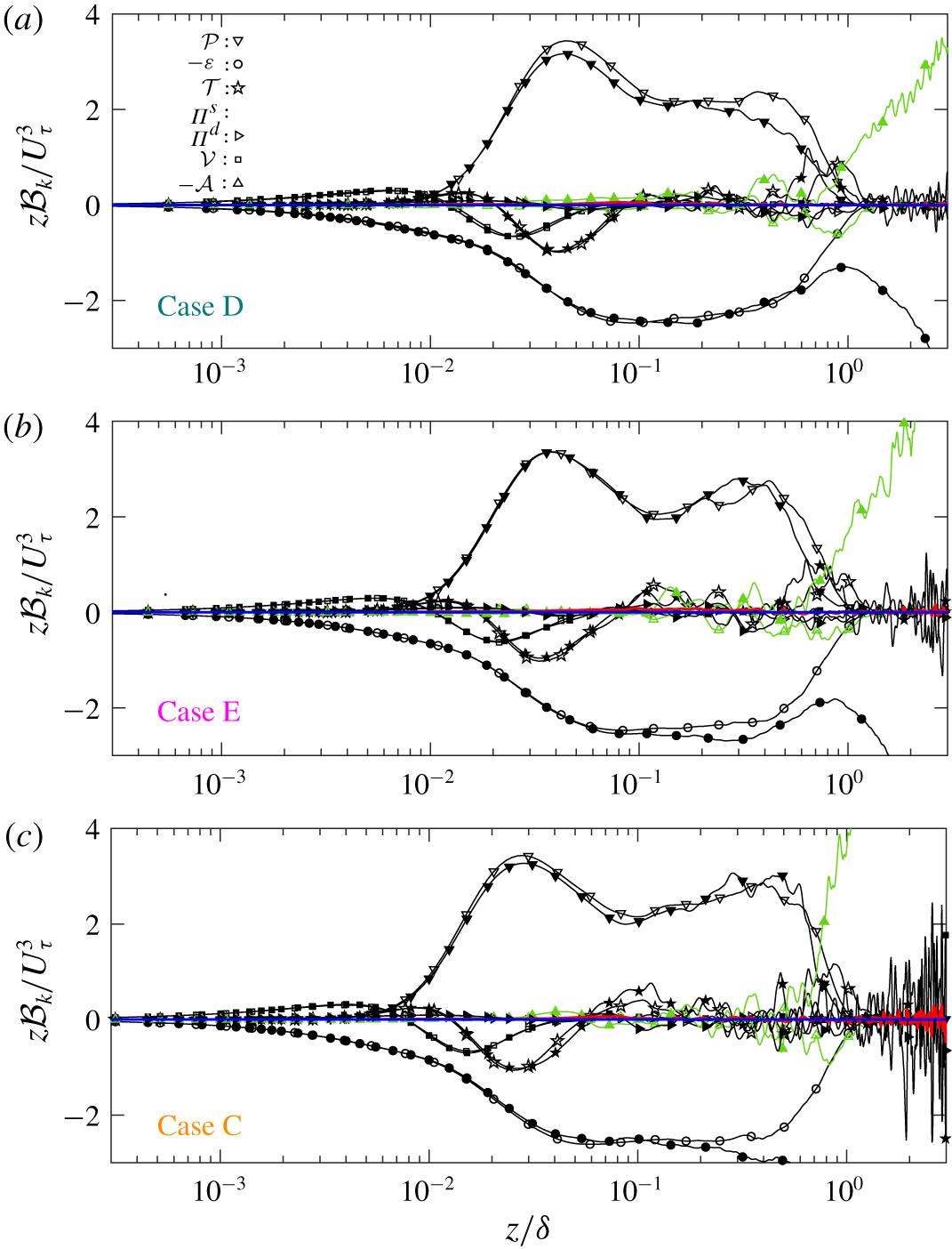
Despite a lack of statistical convergence for curves of the budget terms in figure 14, deduced from single fields at a specific time, we are nonetheless able to assess how the FST has broadly changed, or not changed, the various components of the budget for the different cases throughout the extent of the boundary layer. Similar curves for the quiescent boundary layer (Kozul et al. Reference Kozul, Chung and Monty2016) at matched  $Re_{\unicode[STIX]{x1D70F}}$ are plotted in figure 14 for comparison. The present simulations are shown to be numerically very well converged since the budget residual (red line) is almost zero in all of the cases. It is immediately clear that changes to the boundary layer due to FST injection are restricted to the outer region. Beyond $z\approx \unicode[STIX]{x1D6FF}$, in the absence of production, the turbulence is simply decaying and therefore balanced only by the unsteady term (highlighted in green). This is similar to the balance for the wake embedded in HIT of Pal & Sarkar (Reference Pal and Sarkar2015) at late times when the production term had decayed. The transport term follows that of the quiescent boundary layer and is negative up until $z/\unicode[STIX]{x1D6FF}\approx 0.08$, meaning the FST does not change the boundary layer’s transport of kinetic energy outward from the wall over this region. This is also similar to that found by Pal & Sarkar (Reference Pal and Sarkar2015), where their FST was similarly not strong enough to overcome the transport of turbulence from the wake core outward. Case D shows a consistent decrease of its production term over $z/\unicode[STIX]{x1D6FF}\approx 0.03{-}1$, whereas the effect is less conclusive for cases E and C.
An increase of the unsteady term  $-{\mathcal{A}}$ within the boundary layer may indicate the penetration of decaying FST into it. This term is close to zero throughout the boundary layer in the quiescent case shown for reference, tends to be slightly negative at the edge of it and then zero in the quiescent free stream. For the present FST cases, this term shows a positive shift at the edge of the boundary layer for all the cases, consistent with the large positive value of $-{\mathcal{A}}$ in the free stream (since the curves are shown at the same time post-FST injection, the unsteady term ${\mathcal{A}}$ has the same value relative to $U_{\infty }^{3}$ for all cases shown in figure 14; however, the scale $U_{\unicode[STIX]{x1D70F}}$ differs considerably between cases D, E and C due to their being at different $Re_{\unicode[STIX]{x1D70F}}$). Despite some subtle changes in the outer part of the boundary layer, figure 14 suggests the inner region is largely immune to the effects of the injected FST; the kinetic energy budget close to the wall remains similar to that of the quiescent boundary layer at matched $Re_{\unicode[STIX]{x1D70F}}$. This aligns with previous results herein indicating the FST–boundary layer interaction to be largely restricted to the outer region of the boundary layer.
5 When can the FST change the boundary layer?
The present work attempts to elucidate if and how the fully turbulent boundary layer is changed by free-stream disturbances by observing its development under decaying HIT injected into its free stream. In conducting simulations of boundary layers exposed to FST, we found examples of both ‘strong’ (e.g. case D) and ‘weak’ (e.g. case C) interactions. The ‘weak’ interaction of case C did not show the characteristic suppression of the wake in the mean streamwise velocity profile (Blair Reference Blair1983b; Thole & Bogard Reference Thole and Bogard1996), evident in all other cases, although firm conclusions are precluded by the limited timespan available for that simulation. Case C also displayed less flattening of its intermittency profile, defined on the passive scalar released at the wall, than the other cases. This is despite high FST intensity  $u_{e}^{\prime }/U_{\unicode[STIX]{x1D70F}}$ at injection. That is, the strength, or result, of the interaction cannot be solely predicted from knowledge of the FST intensity (or relative large-eddy length scale ratio $L_{e}^{u}/\unicode[STIX]{x1D6FF}$) in isolation. Doing so may lead to inconsistencies in reported changes to Reynolds stress profiles as suggested from the summary of experimental results of this problem presented in Nagata et al. (Reference Nagata, Sakai and Komori2011).
Changing relative time scale  $e$ on the regime diagram. Coloured curves as per table 2. (a) Regime diagram of figure 7(a) with grey lines of constant $e=(u_{e}^{\prime }/L_{e}^{u})/(U_{\unicode[STIX]{x1D70F}}/\unicode[STIX]{x1D6FF})=T_{\unicode[STIX]{x1D6FF}}/T_{e}$ added, value noted at top right of each line: ●, Hancock & Bradshaw (Reference Hancock and Bradshaw1983); $\times$, Dogan et al. (Reference Dogan, Hanson and Ganapathisubramani2016). (b) Regime diagram showing evolution of $e$ directly as a function of FST intensity $u_{e}^{\prime }/U_{\unicode[STIX]{x1D70F}}$: ●, points at which the interaction becomes ‘weak’, corresponding to the same marked points on figure 8(d); – – –, hypothetical evolution of $e$ formed from $T_{\unicode[STIX]{x1D6FF}}$ of precursor simulations continued without FST injection (as in figure 8) and $T_{e}$ from the corresponding FST cases.
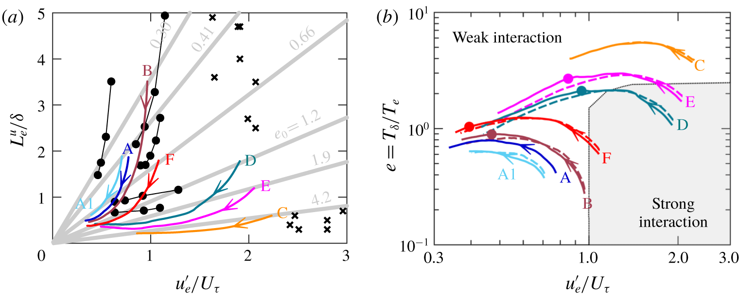
Flattened intermittency profiles were observed for all other cases thus increasing  $\unicode[STIX]{x1D6FF}$, the 99 % boundary layer thickness. The present technique of ‘marking’ boundary layer fluid with a passive scalar reveals large excursions of boundary layer fluid of the order of $2\,\unicode[STIX]{x1D6FF}$ for strongly interacting case D (figure 6d). This significant redistribution of the boundary layer would be otherwise underestimated given the more subtle increase in $\unicode[STIX]{x1D6FF}$. A more spread-out boundary layer with a similar momentum deficit will presumably allow more incursions of FST from the free stream, as was shown in intermittency weighted averaged profiles in § 4.6, where we were able to discern free-stream versus boundary layer contributions to the wall-normal Reynolds stress profiles by conditioning Reynolds stress statistics on the scalar released at the wall. We found that the boundary layer in case C (‘weak’ interaction) was indeed receiving contributions from the FST, but that they did not penetrate deeply as quickly in time as those for cases D and E (‘strong’ interactions). Such incursions then serve to alter the velocity variance profiles, such that they are closer in value to that of the FST. We suggest that in case C, the FST decays more rapidly than the rate at which the boundary layer is able to absorb changes in its velocity profiles. Furthermore, increases in the outer region of velocity variance profiles are only observed when the isotropic $u_{e}^{\prime }/U_{\unicode[STIX]{x1D70F}}$ of the FST differs significantly from the variance profiles of the outer region of the wall-generated turbulence profiles. Looking at, say, $z/\unicode[STIX]{x1D6FF}\approx 0.5$ in figure 13, the gain over the reference quiescent cases (grey curves) for the total or conventionally averaged $\overline{w^{\prime 2}}/U_{\unicode[STIX]{x1D70F}}^{2}$ profiles is larger for all cases at an earlier time (figure 13d–f) when the FST intensity is stronger. Profiles deviate less from the quiescent boundary layer profiles at a later time when the FST has decayed significantly (figure 13g–i). In the literature, increases in the peak of the velocity variance profiles have only been shown when $u_{e}^{\prime }/U_{\unicode[STIX]{x1D70F}}$ of the FST is greater than the peak variance that would be otherwise observed in a boundary layer forming under a quiescent free stream (Thole & Bogard Reference Thole and Bogard1996; Dogan et al. Reference Dogan, Hanson and Ganapathisubramani2016).
Figure 15(a) adds lines of constant  $e=(u_{e}^{\prime }/L_{e}^{u})/(U_{\unicode[STIX]{x1D70F}}/\unicode[STIX]{x1D6FF})=T_{\unicode[STIX]{x1D6FF}}/T_{e}$, a measure of the relative large-eddy time scales in the present temporal interpretation, to the regime diagram of figure 7(a). As stated above, the main action of the FST on the turbulent boundary layer is to increase the rate of its spread away from the wall, which will then serve to increase the boundary layer thickness $\unicode[STIX]{x1D6FF}$ faster than the ${\sim}t^{[0.71,0.73]}$ observed for the quiescent temporal boundary layer of Kozul et al. (Reference Kozul, Chung and Monty2016), which we indeed see in figure 8(a) for most of the present cases. Short temporal ranges mean the exponents are somewhat unreliable yet a range of increased exponents ${\sim}t^{[0.77,0.80]}$ is found for the present FST cases. This is related to the increased spreading rate for the boundary layer due to FST, an effect found to be stronger for both smaller $e_{0}$ and higher FST intensity (figure 8d). An analysis of relevant scales in this problem led to the estimate $e\sim t^{0}$ (2.5), suggesting $e$ would tend to a constant at large $t$ for non-interacting flows. An increased development rate of $\unicode[STIX]{x1D6FF}$ for a ‘strong’ FST–boundary layer interaction will make the exponent on $t$ more positive. Figure 15(b) plots the evolution of $e$ for the present cases against FST intensity $u_{e}^{\prime }/U_{\unicode[STIX]{x1D70F}}$. All cases demonstrate an increase of $e$ in time, before decreasing again. Note that in the present simulations, the increase in $e$ as shown in figure 15(b) is partly attributable to the decrease in $L_{e}^{u}$ for early times in excess of that suggested by power-law fits (figure 3b). In figure 8(d) we marked the points in time at which we deemed the boundary layer–FST interaction had become ‘weak’ (decrease of boundary layer spreading rate back to that for the boundary layer developing under a quiescent free stream) for cases B, D, E and F. Those same points are marked with filled circles in figure 15(b), indicating from which point ‘weak’ interactions presumably begin.
We point to the difference in  $e_{0}=T_{\unicode[STIX]{x1D6FF},0}/T_{e,0}$ when the flows are combined: this quantity differed by a factor of 3 for the two cases C and D that had similar FST intensities at injection. All other things being equal, a different value in $e_{0}$ can arise due to a large difference in the relative length scale $L_{e}^{u}/\unicode[STIX]{x1D6FF}$, although this does not alone appear to be the critical factor in predicting a ‘strong’ or ‘weak’ interaction. In figure 13(d), a strong interaction continues for case D despite $L_{e}^{u}/\unicode[STIX]{x1D6FF}=0.53$ ( $e\approx 2$ at this point in time for case D). This length scale ratio is roughly equal to the $L_{e,0}^{u}/\unicode[STIX]{x1D6FF}_{0}=0.54$ for the weakly interacting case C at FST injection. Since we find a systematic weakening of the effect between cases D ( $e_{0}=1.2$) and E ( $e_{0}=1.9$), we are led to believe that $e_{0}\lesssim 2$ is required for the FST to have sufficient time to strongly interact with the boundary layer. We suggest that if a boundary layer–HIT system satisfies this condition, a ‘strong’ interaction will ensue. We have tentatively shaded a region of the regime diagram in figure 15(b) as giving rise to ‘strong’ interactions. The curve of case B is excluded since, although there is apparently scope for the boundary layer and FST to interact temporally, the FST is not sufficiently strong to cause significant changes to velocity variance profiles (figure 12c). That is, in addition to the condition on $e_{0}$ ensuring that the boundary layer has sufficient time to adjust to the presence of the FST, the FST intensity $u_{e}^{\prime }/U_{\unicode[STIX]{x1D70F}}$ must also be significant compared to the (peak of the) quiescent velocity variance profiles. The Reynolds numbers of both the turbulent boundary layer and the HIT must presumably be sufficiently high for this inertial criterion to be meaningful. Although we could foresee some Reynolds number effects on the borders of the regime, we expect the essence of the argument on relative time scales to hold.
6 Summary
Bradshaw (Reference Bradshaw1996) noted the importance of parameter  $e$ for correlating results for this physical problem over a limited range of FST intensities and length scales, yet at the time it was unclear how general this dependence might be. The present simulations reaffirm the importance of this parameter in predicting the strength of the boundary layer–FST interaction by presenting a limited parametric study of the temporally developing parameter $e$. Furthermore, for the range of parameters and Reynolds numbers we have here studied, it would be possible to gauge in advance whether or not given HIT will impart change onto a turbulent boundary layer developing beneath it. If the large-eddy turnover time scale of the boundary layer is much larger than that of the FST, then the injected FST will decay to negligible levels before the boundary layer is able to ‘notice’ it. The ‘inactive’ FST fluid does not penetrate closer to the wall than around $z^{+}\approx 100$ in such a case. Thus a ‘weak’ interaction could be predicted where a boundary layer’s large-eddy turnover time scale is much larger than that of the FST. Since resulting velocity variance profiles appear approximately as the sum of the FST intensity weighted by the intermittency $\unicode[STIX]{x1D6FE}$ and that for a boundary layer developing under a quiescent free stream, FST intensities must in addition be at least comparable to the peak values of the Reynolds stress profiles for significant change to eventuate. Hancock & Bradshaw (Reference Hancock and Bradshaw1989) found conditionally sampled statistics showed a dependence on $(u_{e}^{\prime }/L_{e}^{u})/(U_{\unicode[STIX]{x1D70F}}/\unicode[STIX]{x1D6FF})=e$, identifying it as a relative fluctuating strain. However, they found that at $e\gtrsim 1$, statistics became markedly less dependent on this parameter. Whilst this implies that the FST has a large relative fluctuating strain compared to the boundary layer, making this, according to such an interpretation, ‘unexpected’, considering it here as a relative large-eddy turnover time scale, we offer an alternative physical explanation: that a large $e$ means that the FST will decay rather more rapidly than the boundary layer is apparently able to adjust to or absorb its effects. Furthermore, Hancock & Bradshaw (Reference Hancock and Bradshaw1989) did not have the capability to observe co-evolution of the boundary layer and the FST, and were unable to untangle history versus contemporaneous effects. Our temporal approach exposes the dynamism of the boundary layer–FST interaction whose inherent nature will be neglected by an equilibrium model. Despite the advantages of the present temporal model in understanding this interaction, it must be borne in mind that the temporal boundary layer is equivalent to the spatial boundary layer only in the asymptotic limit of large Reynolds number. The (vanishing) difference in entrainment due to the small wall-normal velocity at the edge of the spatial boundary layer, absent in the temporal case, means a potential discrepancy exists between the present simulations and their spatial equivalents with regards to entrained fluid from the free stream.
For the present simulations, the relative time scale interpretation, combined with a condition on the FST intensity  $u_{e}^{\prime }/U_{\unicode[STIX]{x1D70F}}$, yields a consistent explanation of our results for the Reynolds number range we have been able to tackle. The ability of the FST to change the boundary layer requires the boundary layer to have time – measured in its own time – to be altered by it. Our present temporal investigation sheds light on the conditions under which the boundary layer is able to ‘see’ the injected free-stream disturbances, before they fade away.
Acknowledgements
Funding provided by the Australian Research Council over the course of M.K.’s doctoral studies is gratefully acknowledged. The Australian Bicentennial Scholarship (Kings College London) and the Diane Lemaire Scholarship (Melbourne School of Engineering) funded M.K.’s study trip to the University of Southampton. This research was partly undertaken on the NCI National Facility in Canberra, Australia, which is supported by the Australian Government. This work was also supported by resources provided by the Pawsey Supercomputing Centre funded by the Australian Government and the Government of Western Australia. Additional simulations were performed on resources provided by UNINETT Sigma2 – the National Infrastructure for High Performance Computing and Data Storage in Norway.
Declaration of interests
The authors report no conflict of interest.


 Open access