


1. Introduction
The understanding of turbulent thermal convection is of great importance for astrophysics, geophysics, climate research and engineering purposes alike. Although convection has been under investigation for centuries, even today researchers struggle to unveil its complex nature. Usually, to study turbulent thermal convection, a model system is considered, where the fluid is confined between horizontal plates heated from below and cooled from above, commonly known as Rayleigh–Bénard convection (RBC) (Bodenschatz, Pesch & Ahlers Reference Bodenschatz, Pesch and Ahlers2000; Ahlers, Grossmann & Lohse Reference Ahlers, Grossmann and Lohse2009; Chillà & Schumacher Reference Chillà and Schumacher2012). In this work we study a different model system, where the fluid is confined between vertical heated/cooled plates, also known as convection inside a differentially heated enclosure, side-heated convection or vertical convection. Throughout this work, we will refer to this system as vertical convection (VC).
RBC and VC are two limiting cases of the more general type of inclined convection (Daniels, Wiener & Bodenschatz Reference Daniels, Wiener and Bodenschatz2003; Chillà et al. Reference Chillà, Rastello, Chaumat and Castaing2004; Sun, Xi & Xia Reference Sun, Xi and Xia2005; Ahlers, Brown & Nikolaenko Reference Ahlers, Brown and Nikolaenko2006; Weiss & Ahlers Reference Weiss and Ahlers2013; Shishkina & Horn Reference Shishkina and Horn2016; Zwirner & Shishkina Reference Zwirner and Shishkina2018; Zwirner et al. Reference Zwirner, Khalilov, Kolesnichenko, Mamykin, Mandrykin, Pavlinov, Shestakov, Teimurazov, Frick and Shishkina2020a) and therefore are of particular importance. Note, that VC, unlike RBC, is inherently unstable even for the smallest temperature difference between the plates.
Batchelor (Reference Batchelor1954) was one of the first to investigate VC for very small temperature differences, and, in the beginning, the main interest was in studying the heat transport through double layer windows. Therefore, the studied geometry was of very large aspect ratio  $L_z/H$, where $L_z$ is the height of the convection cell and $H$ is the distance between the heated and cooled vertical plates. Fujii et al. (Reference Fujii, Takeuchi, Fujii, Suzaki and Uehar1970) performed a detailed experimental study on the evolution of boundary layers (BLs) and local heat transport in VC, using two concentric cylinders, where the inner one was heated and the outer one cooled, and using oil and water as working fluids. Belmonte, Tilgner & Libchaber (Reference Belmonte, Tilgner and Libchaber1995) used a cubic cell and different gases of Prandtl number $\textit {Pr}\approx 0.7$ for Rayleigh numbers ${\textit {Ra}}_H\leq 10^{11}$ and found by shadowgraph visualization a stably stratified bulk, while the temperature fluctuations were mainly observed close to the boundaries. Additionally, they measured a scaling of the thermal BL thickness $\sim {\textit {Ra}}^{-0.29}$. Koster, Seidel & Derebail (Reference Koster, Seidel and Derebail1997) used X-ray radiography to measure and visualize the density distribution inside a narrow VC cell filled with liquid gallium. This was a milestone in the visualization of liquid metal flows, however, it is only applicable to narrow cavities and also no conclusions about turbulent convection could be drawn. Braunsfurth et al. (Reference Braunsfurth, Skeldon, Juel, Mullin and Riley1997) conducted experiments with liquid gallium inside a long VC cells of aspect ratios $L/H=1/3$ and $1/4$, for small Grashof numbers ( ${\textit {Ra}}/\textit {Pr}<5\times 10^4$) and compared the results with two-dimensional numerical simulations. Here, we investigate flow at much larger ${\textit {Ra}}$ and large aspect ratios.
As in RBC (Shishkina Reference Shishkina2021), in VC, the aspect ratio of the container influences the flow in a finite fluid layer confined between two differently heated plates (Batchelor Reference Batchelor1954; Bejan Reference Bejan1980, Reference Bejan1985, Reference Bejan2013; Paolucci Reference Paolucci1994). However, the effects of the container's size and the distance between its walls have not been investigated separately. Understanding this phenomenon is of special significance in convection, especially in a small- $\textit {Pr}$ fluid, as both these length scales influence the flow field. In particular, this sort of flow configuration is typically encountered in liquid metal batteries (Kelley & Weier Reference Kelley and Weier2018) – a technology with potential in grid-scale storage. In this paper, we attempt to disentangle the aspect ratio dependency, and shift the focus onto the two predominant length scales using numerical and experimental data across several aspect ratios. Additionally, we also present a robust new technique which is capable of computing the Reynolds number based on the wind velocity.
There are only a few examples of ongoing investigations of VC and in addition to Churchill & Chu (Reference Churchill and Chu1975); Graebel (Reference Graebel1981); Tsuji & Nagano (Reference Tsuji and Nagano1988); Chen & Pearlstein (Reference Chen and Pearlstein1989); Paolucci (Reference Paolucci1990); Versteegh & Nieuwstadt (Reference Versteegh and Nieuwstadt1999); Pallares et al. (Reference Pallares, Vernet, Ferre and Grau2010); Kis & Herwig (Reference Kis and Herwig2012) and Wang et al. (Reference Wang, Liu, Verzicco, Shishkina and Lohse2021); there are even more studies, but most of them use air, oil or water with relatively large Prandtl numbers,  $Pr\gtrsim 0.7$. However, recently, liquid metals with very small Prandtl numbers, $\textit {Pr}\ll 1$, have become a particular focus of investigations in the thermal convection community (King & Aurnou Reference King and Aurnou2013; Scheel & Schumacher Reference Scheel and Schumacher2016; Schumacher et al. Reference Schumacher, Bandaru, Pandey and Scheel2016; Aurnou et al. Reference Aurnou, Bertin, Grannan, Horn and Vogt2018; Vogt et al. Reference Vogt, Horn, Grannan and Aurnou2018a; Zwirner & Shishkina Reference Zwirner and Shishkina2018; Zürner et al. Reference Zürner, Schindler, Vogt, Eckert and Schumacher2019; Zwirner et al. Reference Zwirner, Khalilov, Kolesnichenko, Mamykin, Mandrykin, Pavlinov, Shestakov, Teimurazov, Frick and Shishkina2020a; Zwirner, Tilgner & Shishkina Reference Zwirner, Tilgner and Shishkina2020b). The aim of the present work is to shed more light on VC of low-Prandtl-number fluids.
One important step that led to a better understanding of RBC was the development of the scaling theory by Grossmann & Lohse (Reference Grossmann and Lohse2000, Reference Grossmann and Lohse2002) (GLT). This theory is based on the exact relationships between the heat transport, represented by the dimensionless Nusselt number  ${\textit {Nu}}$, and the kinetic and thermal dissipation rates. The GLT assumes various scaling regimes ( ${\textit {Nu}}\sim {\textit {Ra}}^\gamma$) depending on which part of the flow determines the scalings of the dissipation rates: the BLs or the bulk. This theory also concludes that there is no simple scaling law applicable for the entire range of Rayleigh numbers, but that the exponent $\gamma$ changes smoothly within these regimes. A similar approach has been applied by Ng et al. (Reference Ng, Ooi, Lohse and Chung2015) to VC, however, the difficulty in this case is a non-closed term in the relationship between ${\textit {Nu}}$ and the kinetic energy dissipation rate. Nevertheless, Ng et al. (Reference Ng, Ooi, Lohse and Chung2015) concluded that a similar approach to the GLT is applicable to VC, when a suitable closure model for that specific term is found.
Although one might deem the question about which scales determine the flow settled, there is still active research on the most suitable scales. For example, Wei (Reference Wei2020) found the proper scale for the Reynolds shear stress in a differentially heated vertical channel is a mixed scale of the friction and the maximum mean velocity.
Scaling relations for heat transport and BL thicknesses in vertical convection have been investigated in the past (Batchelor Reference Batchelor1954; Gill Reference Gill1966; Saville & Churchill Reference Saville and Churchill1969; Ostrach Reference Ostrach1972). A recent approach agrees upon the same exponents for vertical convection in the laminar regime, there the exponents were derived from BL theory and confirmed by direct numerical simulations (DNS) in a theoretical work (Shishkina Reference Shishkina2016).
It was found that for  $\textit {Pr}\ll 1$ the Nusselt number and the wind-based Reynolds number scale with respect to the Rayleigh and Prandtl numbers as
 \begin{equation} {\textit{Nu}}\sim\textit{Pr}^{1/4}{\textit{Ra}}^{1/4}\quad\text{and}\quad\textit{Re}_{wind}\sim\textit{Pr}^{{-}1/2}{\textit{Ra}}^{1/2}, \end{equation}
respectively. Note that the scaling relations are valid regardless of the length scale chosen and therefore the indices  $H$ and $L$ are omitted. However, the pre-factor depends on this choice and in the following we show that the data collapse for different aspect ratios when the scale is chosen appropriately.
The remaining article is structured as follows: in § 2 we introduce the experimental and numerical set-up, in § 3 we present a detailed comparison of the experimental and numerical results and discuss the relevant length scale, heat and momentum transport and finally we conclude with § 4.
2. Experimental and numerical methods
Here, we present our numerical and experimental methods. A sketch of the basic set-up used in the experiments and the three-dimensional DNS is shown in figure 1. We use a rectangular cell with variable aspect ratio,  $L/H$, where the heated and cooled plates are squares of length $L=L_y=L_z$. The distance between the heated and cooled plates is $H$.
$H$.
Sketch of the VC cell with a heated wall at the left side (temperature  $T_+$) and cooled wall at the right side (temperature $T_-$). The velocity is measured along two lines parallel to the $z$-direction, using the Doppler probes $A$ and $B$. The direction of gravity is indicated by $\boldsymbol {g}$. This sketch represents the set-up for the DNS as well as the experiments.

2.1. Numerical set-up
The incompressible Navier–Stokes equations in Oberbeck–Boussinesq approximation
 \begin{gather} D_t \boldsymbol{u} = \nu{\nabla}^2 \boldsymbol{u} -\boldsymbol{\nabla} p + \alpha g (T-T_0) \hat{\boldsymbol{z}}, \end{gather}
 \begin{gather}D_t T = \kappa {\nabla}^2 T, \end{gather}
 \begin{gather}\boldsymbol{\nabla} \boldsymbol{\cdot} \boldsymbol{u} = 0 \end{gather}
are solved using the high-order finite volume code Goldfish (Kooij et al. Reference Kooij, Botchev, Frederix, Geurts, Horn, Lohse, van der Poel, Shishkina, Stevens and Verzicco2018) in Cartesian coordinates. Here,  $D_t$ denotes the substantial derivative, $\boldsymbol {u} = (u_x, u_y, u_z)$ the velocity vector field, $p$ is the reduced kinetic pressure, $T$ the temperature, $T_+$ the temperature of the hot vertical plate, $T_-$ the temperature of the cold vertical plate, $T_0$ is the mean temperature $(T_++T_-)/2$, $\nu$ is the kinematic viscosity and $\kappa$ the thermal diffusivity. The equations are transformed into their non-dimensional representation using the distance $H$ between the hot and cold plates, the time $t_f\equiv H(\alpha gH\varDelta )^{-1/2}$ and the temperature difference $\varDelta \equiv T_+-T_-$, g is the gravitational acceleration. Thus, our VC system depends on the following three non-dimensional input parameters:
 \begin{equation} {\textit{Ra}}_H\equiv \alpha g \Delta H^3/(\kappa \nu), \quad\textit{Pr}\equiv \nu/\kappa, \quad\varGamma=L/H, \end{equation}
which are the Rayleigh number, Prandtl number and aspect ratio, respectively. All DNS are conducted at  $\textit {Pr}=0.03$.
The computational mesh, used in the simulations, is clustered near the boundaries and the largest simulation ( ${\textit {Ra}}_H=10^8$ and $\varGamma =1$) has a resolution of $674^3$ points, while the averaging time is usually $t_{avg}\geqslant 150\,t_f$. We start to collect the statistics after the flow reaches a stationary state as indicated by the fluctuations of ${\textit {Nu}}(t)$ around a constant long-time average. The number of points within the viscous BL is always $N_{\delta _u}\geqslant 4$ and due to the small Prandtl number, the thermal BL is much thicker than the viscous one and therefore both BLs are well resolved. Additionally, we conducted a mesh convergence study and also ensure that our typical mesh distance $h$ resolves the Kolmogorov scale $\eta =(\nu ^3/\varepsilon _u)^{1/4}$ (where $\varepsilon_u$ is the kinetic energy dissipation rate), i.e. $h\lesssim \eta$, which represents the smallest scales of the flow. A detailed list of the DNS resolution can be found in the Appendix, table 1.
Simulation parameters: the aspect ratio ( $L/H$), Rayleigh number ( ${\textit {Ra}}_H$), grid size ( $N_x\times N_y\times N_z$), averaging time ( $T_{avg}$) and number of points in the viscous ( $N_{\delta _u}$) and thermal BLs ( $N_{\delta _\theta }$). The Prandtl number is fixed to $\textit {Pr}=0.03$.

Important characteristic output quantities in VC are the Nusselt number, the Reynolds number and the thermal/viscous BL thicknesses. The Nusselt number represents the heat transport through the system and is defined as
 \begin{equation} {\textit{Nu}}_H\equiv\frac{\langle\overline{u_xT}-\kappa\partial_x\bar{T}\rangle_{A_{yz}}}{\kappa\varDelta/H}, \end{equation}
where  $\langle \cdot \rangle _{A_{yz}}$ means averaging over a slice parallel to the hot plate and $\bar {\cdot }$ averaging over time. The thickness of the thermal BL is defined as usual: $\delta _\theta \equiv H/(2{\textit {Nu}})$. For the definition of the Reynolds number, we follow Shishkina (Reference Shishkina2016) and introduce the wind velocity in a similar manner as
 \begin{equation} U_{wind}\equiv \max_{x}\left\lbrace\langle\overline{u_z}\rangle_{A_{yz}}\right\rbrace, \end{equation}
and with this the wind-based Reynolds number
 \begin{equation} \textit{Re}_{wind} = \frac{LU_{wind}}{\nu}. \end{equation}
Furthermore, we define the thickness of the viscous BL using the slope method (Zhou & Xia Reference Zhou and Xia2010)
 \begin{equation} \delta_u\equiv \frac{U_{wind}}{\partial_x \langle\overline{u_z}\rangle_{A_{yz}}\vert_{x=0}}. \end{equation}
Note that, for laminar flow,  $\delta _u\sim \textit {Re}^{-1/2}$, and using (1.1) we conclude that $\delta _u\sim {\textit {Ra}}^{-1/4}$. For an example of the horizontal profile $\langle \overline {u_z}\rangle$ we refer the reader to figure 8(c,d).
2.2. Laboratory set-up
Figure 1 shows a schematic drawing of the experimental set-up. The experiments were performed in two rectangular vessels with a square vertical cross-section of  $L^2 = 200\ \textrm {mm}\times 200\ \mathrm {mm}$ and a distance between the vertical heated/cooled boundaries of $H=40$ and $H=66\ \mathrm {mm}$, which gives aspect ratios of $\varGamma = L/H = 5$ and $\varGamma \approx 3$, respectively. On the two square vertical surfaces of the vessel, the heat is introduced and removed via two copper plates, which are tempered by a circulating water bath and the temperature is controlled via thermocouples inside the copper plates.
The maximal thermal power input is  $P=1500$ W in this study. The other sidewalls are made of 30 mm thick Polyvinylchloride. To minimize heat losses, the whole convection cell is wrapped in a 30 mm thick closed-cell foam, which has a thermal conductivity of approximately $0.036\ \textrm {W}\ \textrm {mK}^{-1}$ and is ${\sim }660$ times lower that of the liquid metal ( $24\ \textrm {W}\ \textrm {mK}^{-1}$).
The vessel is filled with the eutectic alloy GaInSn that has a melting temperature of  $T_s = 10.5\,^\circ \textrm {C}$. At room temperature, it has the density $\rho = 6350 \ \mathrm {kg}\ \mathrm {m}^{-3}$, the thermal expansion coefficient $\alpha = 1.24 \times 10^{-4}\ \mathrm {1}\ \mathrm {K}^{-1}$, the thermal conductivity $\lambda = 24.05\ \mathrm {W}\ \mathrm {mK}^{-1}$, the kinematic viscosity $\nu = 3.38 \times 10^{-7}\ \mathrm {m}^2\ \mathrm {s}^{-1}$ and the thermal diffusivity $\kappa = 1.05 \times 10^{-5} \ \mathrm {m}^2\ \mathrm {s}^{-1}$ (Plevachuk et al. Reference Plevachuk, Sklyarchuk, Eckert, Gerbeth and Novakovic2014). The corresponding Prandtl number is $Pr\approx 0.03$.
For the majority of the measurements, we keep the mean fluid temperature constant at approximately  $21\,^{\circ }\textrm {C}$. Only for the highest ${\textit {Ra}}$ do we have to increase the mean fluid temperature up to $35\,^{\circ }\textrm {C}$. However, the temperature dependence of the material parameters is comparatively low, thus the Prandtl number changes only by approximately 10 % ( $2.97 \leq Pr/10^{-2} \leq 3.25$). Therefore, we consider possible non-Oberbeck–Boussinesq effects to have a rather weak influence on the flow.
2.3. Measuring technique
In this study, the flow velocities are measured using ultrasonic Doppler velocimetry (UDV) which is an established measurement technique for opaque fluids like liquid metals (Aubert et al. Reference Aubert, Brito, Nataf, Cardin and Masson2001; Brito et al. Reference Brito, Nataf, Cardin, Aubert and Masson2001; Eckert & Gerbeth Reference Eckert and Gerbeth2002; Gillet et al. Reference Gillet, Brito, Jault and Nataf2007; Nataf et al. Reference Nataf, Alboussiere, Brito, Cardin, Gagnière, Jault and Schmitt2008; Vogt, Räbiger & Eckert Reference Vogt, Räbiger and Eckert2014; Vogt et al. Reference Vogt, Horn, Grannan and Aurnou2018a,Reference Vogt, Ishimi, Yanagisawa, Tasaka, Sakuraba and Eckertb; Zürner et al. Reference Zürner, Schindler, Vogt, Eckert and Schumacher2019, Reference Zürner, Schindler, Vogt, Eckert and Schumacher2020; Yang, Vogt & Eckert Reference Yang, Vogt and Eckert2021; Vogt, Horn & Aurnou Reference Vogt, Horn and Aurnou2021a; Vogt et al. Reference Vogt, Yang, Schindler and Eckert2021b). The used UDV system is a DOP3010 (from Signal Processing SA, Lausanne) equipped with 8 MHz transducers. The UDV transducers send a pulsed ultrasonic signal into the liquid metal which is reflected by microscopic particles such as oxides. The position and velocity of the particles can be determined from the transit time of the ultrasound and the phase shift of the echo from subsequent echo pulses. This allows us to determine the beam-parallel velocity distribution along the ultrasonic beam (Takeda Reference Takeda2012). The two ultrasonic sensors used in this study measure velocities along the vertical direction (cf. figure 1). The distances from the sensors to the heated plate are  $x_{p}/H = 0.25$ and $0.75$ for $\varGamma =5$, and $x_{p}/H = 0.15$ and $0.85$ for the $\varGamma =3$. The measuring system records velocity profiles with a time resolution of approximately 0.3 s. The spatial resolution is approximately 1 mm in the beam direction and 5 mm in the lateral direction due to the diameter of the ultrasound emitting piezoelectric transducer.
The experiment is equipped with  $22$ thermocouples with nine being embedded in each copper plate to measure the temperature drop across the fluid layer. The remaining four thermocouples are attached to the water channels that temperate the copper plates, in order to determine the temperature change of the circulating water ( $T_{in} - T_{out}$). Together with the measurements of the water flow rate $\dot {V}$, this enables the calculation of the convective heat transport, which is expressed non-dimensionally by the Nusselt number
 \begin{equation} {\textit{Nu}} = \frac{\dot{Q}_{tot}}{\dot{Q}_{cond}} = \frac{\rho c_p \dot{V} (T_{in} - T_{out})}{\lambda L^2 \varDelta / H}, \end{equation}
where  $c_p$ is the isobaric heat capacity of water. There are small differences between the measurements at the hot and cold plates due to thermal losses. The Nusselt numbers presented here are the averages of the hot and cold measurement ( $\varGamma =5$), or shown separately ( $\varGamma =3$).
2.4. Extraction of the Reynolds number
One objective of this work is to compare the simulations with the experiments, and therefore we need to define a Reynolds number based on a certain velocity that is easily measurable in both simulations and experiments. In the experiments, only limited velocity data are available from the UDV probes, while the simulations provide access to the complete velocity fields. Therefore, we can directly compare the two-dimensional velocity fields  $u_z(t, z)$ only at the Doppler probe positions ( $x_{p}/H = 1/4$ and $3/4$). Examples of these data are visualized in figure 2(a,c,e). There are multiple possibilities to define a characteristic velocity based on these data. Here, we investigate two candidates in detail, a straightforward one (the maximal velocity) and a more sophisticated one (based on the autocorrelation) which we define in the following.
Examples of time–space plots of the vertical velocity  $u_z(t, z)$ for: (a) DNS data at probe $A$,
$A$,  $\varGamma =5$, ${\textit {Ra}}_L=1.25\times 10^7$, (c) experimental data at probe $B$,
$B$,  ${\textit {Ra}}_L=1.05\times 10^7$ and (e) noisy experimental data at probe $B$,
$B$,  ${\textit {Ra}}_L=6.94\times 10^6$. (b,d,e) The autocorrelation function $\mathcal {C}_{u_z}(\tau, \zeta )$ for (a,c,e) respectively, cf. (2.12). The dashed lines indicate the characteristic velocity $U^\star$ obtained from the autocorrelation as described in § 2.4.

The maximal velocity is defined as
 \begin{equation} U_{max}\equiv\max_{z}\left\lbrace\overline{u_z(t, z)}\right\rbrace, \end{equation}
and the corresponding Reynolds number
 \begin{equation} \textit{Re}^{max}_L\equiv\frac{LU_{max}}{\nu}. \end{equation}
 A more sophisticated approach is based on the two-dimensional autocorrelation of  $u_z(t, z)$, which we calculate in a discrete manner as
 \begin{equation} \mathcal{C}_{u_z}(\tau, \zeta)=\frac{1}{NM\sigma^2}\sum_{i,j}^{N, M} u^\prime_z(t_i, z_j)\cdot u^\prime_z(t_i-\tau, z_j-\zeta), \end{equation}
where  $u_z^\prime (t, z)\equiv u_z(t, z)-\langle \overline {u_z}\rangle _z$ and $\sigma$ is the standard deviation of $u_z$. Note that, in (2.12), the fraction in front of the sum normalizes $\mathcal {C}_{u_z}$ to values between $-1$ and $1$. Examples of $\mathcal {C}_{u_z}(\tau, \zeta )$ are shown in figure 2(b,d,f). The next step is to fit a straight line,
 \begin{equation} \zeta(\tau) = U^\star\tau \end{equation}
through the points
 \begin{equation} \left\lbrace(\tau_i, \zeta_i) : \mathcal{C}_{u_z}(\tau_i, \zeta_i) = \max_{\tau}\mathcal{C}_{u_z}(\tau, \zeta_i)\right\rbrace. \end{equation}
The slope of this line gives the characteristic velocity  $U^\star$. Additionally, we restrict the domain of the fit to the relevant points around the origin. How this extraction algorithm works with experimental and numerical data is shown by several examples in figure 2. At this point, we can define the Reynolds number based on $U^\star$ as
 \begin{equation} \textit{Re}^\star_L=\frac{LU^\star}{\nu}. \end{equation}
The advantage of evaluating the velocity in this way is that this method provides very robust results even in the case of low-quality signals. Figure 2(e) shows an example of a measurement with a very noisy signal. This is due to weak echo amplitudes caused by an imperfect acoustic contact between the transducer and the liquid metal or an insufficient number of reflective tracers in the measurement volume. In this case, the local velocity values are subject to a high measurement uncertainty, in particular with increasing distance from the sensor. However, the method proposed here uses almost all the available information from the measurements, and by taking into account the spatio-temporal nature of the velocity field, the deficit of poor signal quality can be essentially compensated.
3. Results and discussion
In the following, we will present the results and discuss the evidence, that the relevant length scale in VC is based on the plate size rather than on the distance between the hot and cold plates. Furthermore, we are going to explore the flow structures and BLs, and finally we discuss the new method based on the autocorrelation to determine Reynolds numbers from UDV data. A summary of the measured quantities can be found in the Appendix, tables 2 and 3, however, this is only for reference, as all the quantities are presented in various figures.
Summary of the measured quantities in the DNS for  $\textit {Pr}=0.03$: the aspect ratio ( $L/H$), the Rayleigh number ( ${\textit {Ra}}$) based on $L$ and $H$, the Nusselt number ( ${\textit {Nu}}$), the various Reynolds numbers ( $\textit {Re}$) defined by (2.11), (2.15) and (2.7) and the viscous and thermal BL thicknesses ( $\delta _u$, $\delta _\theta$). Note that $\textit {Re}^\star _L$ and $\textit {Re}^{max}_L$ are the averages of probes $A$ and $B$.
$B$.

Summary of the measured quantities in the experiments: the Rayleigh number ( ${\textit {Ra}}$) based on $L$ and $H$, the Nusselt number ( ${\textit {Nu}}$), and the two Reynolds numbers ( $\textit {Re}$) defined by (2.11) and (2.15). Note that $\textit {Re}^\star _L$ and $\textit {Re}^{max}_L$ are the averages of probes $A$ and $B$. Rows marked by $^{\dagger}$ involve noisy UDV data. The experiments are conducted at $\textit {Pr}\approx 0.03$ and the aspect ratios $L/H=3$ and $5$.
$5$.

3.1. Global flow organization
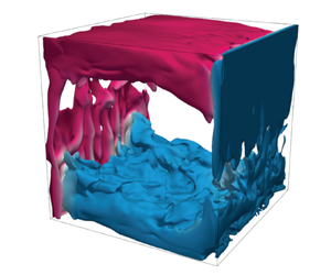
To provide a deeper insight into the general flow organization, we show in figure 3 instantaneous flow fields at different  ${\textit {Ra}}_L$ and aspect ratios $\varGamma$. We calculate the full heat transport vector
 \begin{equation} \boldsymbol{{\varOmega}}\equiv(\boldsymbol{u}T-\kappa\boldsymbol{\nabla} T)/(\kappa\varDelta/H), \end{equation}
and then find regions where its magnitude is greater or equal to the Nusselt number ( $\vert \boldsymbol {{\varOmega }}\vert \geqslant {\textit {Nu}}$). This prominently shows the large-scale circulation and captures the major regions, where heat is transported. Here, we choose the magnitude of the full heat flux vector as the basis and not just the $x$ component. In this way we can capture the regions of vertical heat transport close to the tempered walls and also the heat transport between them. Additionally, this surface is coloured by temperature, to distinguish the hot and cold streams of the flow. This way of visualization helps to overcome two difficulties: on the one hand, vector fields are difficult to render in three dimensions and even streamlines appear rather cluttered, and on the other hand, temperature isosurfaces appear rather smooth due to the low Prandtl number and therefore hide the vigorous nature of turbulent convection in liquid metals.
Instantaneous heat transport and temperature. The shown superstructures enclose regions, where the instantaneous heat transport  $\vert \boldsymbol {\varOmega }(t)\vert \geqslant {\textit {Nu}}$, and they are coloured with the local temperature. Panels (a–c) are at ${\textit {Ra}}_H=5\times 10^4$ and different aspect ratios $\varGamma =1, 2, 5$, respectively. Panels (d,e,c) are at similar ${\textit {Ra}}_L=5\times 10^6, 4\times 10^6, 6.25\times 10^6$, respectively.

3.2. The characteristic length scale
There are two prominent length scales in a rectangular box with square hot/cold plates: the distance  $H$ between the plates and the height of the side hot/cold square plates $L$. One of the questions we are going to answer in this section is: On which length scale ( $H$ or $L$) should the scaling dimensionless quantities like ${\textit {Ra}}$ and $\textit {Re}$ be based?
We denote quantities that are based on  $L$ or $H$ with the subscript $L$ or $H$, respectively, and they convert as
 \begin{equation} {\textit{Ra}}_L= {\textit{Ra}}_H\varGamma^3,\quad{\textit{Nu}}_L= {\textit{Nu}}_H\varGamma\quad\text{and} \quad\textit{Re}_L = \textit{Re}_H\varGamma. \end{equation}
A comparison of the length scales for the Nusselt number is shown in figure 4(a,b) and the data collapse for the length scale  $L$, while they do not do so for length scale $H$. In general, one can see this collapse for the Reynolds numbers in figure 5(a,b) and the BL thickness in figure 6. This means, that the relevant length scale in VC is the plate size, $L$, rather than the plate distance, $H$, for global quantities like ${\textit {Nu}}$ and $\textit {Re}$. Further below, will analyse these quantities and figures in detail.
Nusselt number,  ${\textit {Nu}}$, vs Rayleigh number, ${\textit {Ra}}$, based on length scales: (a) distance of hot and cold plate $H$ and (b) plate length $L$. For $\varGamma =3$ the Nusselt number is measured at the hot plate (red pluses) and at the cold plate (blue pluses). The insets show the compensated Nusselt number based on a ${\textit {Ra}}^{1/4}$-scaling (indicated by dashed lines).

(a) Reynolds numbers based on the characteristic velocity  $\textit {Re}^\star$, and (b) Reynolds numbers based on the maximal vertical velocity vs the Rayleigh number. The data of red/blue triangles (DNS) and crosses/pluses (experiments) are obtained by probes at position $A$/
$A$/ $B$, respectively. The orange background of data points indicates noisy measurements, cf. figure 2(e). The dashed lines show the theoretical scaling $\textit {Re}\sim {\textit {Ra}}^{1/2}$ (Shishkina Reference Shishkina2016) and the grey band represents the uncertainty margin of $\pm 20\,\%$. The wind-based Reynolds numbers $\textit {Re}_{wind}$ from DNS data are shown by grey solid symbols for different aspect ratios $\varGamma =1$ (circle), $2$ (square) and $5$ (triangle). The insets show compensated plots.

Thermal BL thickness  $\delta _\theta =H/(2\,{\textit {Nu}})$ (open symbols, black crosses) and viscous BL thickness $\delta _u$ based on slope criterion (filled symbols, blue crosses, red pluses) vs the Rayleigh number. The dashed and dash-dotted lines show the theoretical scaling law $\delta \sim {\textit {Ra}}^{-0.25}$ for both BLs. The insets show the compensated data. Experimental data for $\varGamma =3$ (pluses) and $\varGamma =5$ the (crosses). DNS data (circles, squares, triangles) as in figure 4.

The Nusselt number for the  $\varGamma =3$ experiments is only ${\approx }70\,\%$ of the value observed in the numerical simulations. Interestingly, this appears to be a systematic difference in liquid metal simulations and experiments. Zwirner et al. (Reference Zwirner, Khalilov, Kolesnichenko, Mamykin, Mandrykin, Pavlinov, Shestakov, Teimurazov, Frick and Shishkina2020a) compare DNS and experiments of VC with liquid sodium as fluid inside a cylinder ( $\varGamma =1$). There, the absolute measurement of ${\textit {Nu}}$ also shows similar differences. Since the DNS results are in agreement with the literature (Scheel & Schumacher Reference Scheel and Schumacher2016), we think this systematic deviation is due to some physical effects not considered within the Navier–Stokes equations, and should be investigated in the future.
As next step, we take a closer look at the local flow organization, which reveals a more complex picture. Here, we focus on the time-averaged heat transport across the central vertical cross-section  $\bar {\varOmega }_x$ (figure 7a) and the respective profile along the vertical direction (figure 7b). The profiles are obtained from the same simulations as the instantaneous snapshots in figure 3. Note that the three red curves correspond to figure 3(d,e,c) and have a similar ${\textit {Ra}}_L$. Although, the slopes of the profiles close to the boundary are similar, the behaviour in the bulk is qualitatively different for different aspect ratios. The smaller aspect ratios, $\varGamma =1$ and $2$, have a steep rise and a steep fall of the heat transport around its maximum close to the wall, where the heat transport is approximately $5$ times larger than the average ${\textit {Nu}}$, while for $\varGamma =5$, the rise and fall are gentle and the maximum is slightly above the average heat transport. The shape of the heat transport profile for the $\varGamma =5$ case shares some similarities with the profiles at smaller aspect ratios $\varGamma =1$ and $2$ for similar ${\textit {Ra}}_H$ (blue curves). Therefore, one may conclude that the local flow organization is strongly influenced by the aspect ratio and the profiles show a rather complex behaviour. This is further supported by the shapes of the time-averaged horizontal profiles of the temperature and vertical velocity component (figure 8).
(a) Cross-section of  $\bar {\varOmega }_x(x=0.5\,H)/{\textit {Nu}}$ for $\varGamma =1$ and ${\textit {Ra}}_H=5\times 10^6$ and (b) profiles of the local heat transport $\bar {\varOmega }_x(x=0.5\,H)$ averaged in the $y$-direction as functions of vertical coordinate $z$. For the red lines $Ra_L\approx 5\times 10^6$ and these data are collected from the same simulations as presented in figure 3(c–e). All DNS data.

Time-averaged horizontal profiles of (a,b) the temperature and (c,d) the vertical velocity component for (a,c)  ${\textit {Ra}}_H=5\times 10^4$ and (b,d) ${\textit {Ra}}_L\approx 5\times 10^6$. All DNS data.

In figure 9 we show the vertical profiles of the thermal BL thickness at the heated plate, for the same cases discussed in the previous paragraph. Here, one notices that, for the same  ${\textit {Ra}}_H$, the profiles are quite different for different aspect ratios (figure 9a), while, for similar ${\textit {Ra}}_L\approx 5\times 10^6$, the thermal BLs are of similar structure (figure 9b). At the top ( $z/L=0$) and bottom ( $z/L=1$) one can prominently notice the influence of the adiabatic boundaries. The thermal BL grows from the bottom to top, first slowly until $z/L\approx 0.7$ and then faster, being influenced by the adiabatic top boundary.
Profiles of the thermal BL  $\delta _\theta /L=-(2\partial _x T)^{-1}$ at the hot plate $x=0$ averaged in the $y$-direction as a function of the vertical coordinate $z$. Note that this definition of $\delta _\theta$ is analogous to $\delta _\theta /L=1/(2{\textit {Nu}})$, and at the plate heat is transported exclusively by conduction; (a) $\varGamma =1, 2, 5$ and ${\textit {Ra}}_H=5\times 10^4$ and (b) $\varGamma =1, 2, 5$ at similar ${\textit {Ra}}_L\approx 5\times 10^6$. The legend is identical to figure 7(b). All DNS data.

3.3. The Reynolds number in experiments and DNS
In § 2.4, we introduced two different methods to extract the Reynolds number and in the following we discuss the robustness of these methods and compare the results from experiments and DNS. We need to take into account that the beam of the Doppler-velocimetry probe has a certain horizontal extent of diameter less than  $H/4$. Analysing the DNS data, we can mimic this horizontal extent by locally averaging over a certain area. Due to the Cartesian geometry used in the simulations, we average over a beam with a square cross-section of area $A_p$ and a side length of up to $H/4$ to account for the finite extent of the Doppler-velocimetry beam.
To verify the robustness of our measurements of the vertical velocity component we separately analyse the influence of two major aspects: (i) the horizontal position of the probe and (ii) the thickness of the ultrasonic beam. The Reynolds number  $\textit {Re}^\star _L$ depends weakly on the horizontal position $x_{p}$ of the probe, while $\textit {Re}^{max}_L$ depends strongly on the horizontal position of the probe (figure 10a). By changing the averaging area of the square beam from our numerical probes in the DNS, we find that the extend of the probing beam has a rather small effect of ${\approx }2\,\%$ on the Reynolds numbers (figure 10b).
Dependence of the normalized Reynolds numbers  $\textit {Re}^{max}_L$ (squares) and $\textit {Re}^\star _L$ (circles) on (a) the horizontal probe position and (b) the beam thickness (represented by the cross-sectional area $A_p$) for the DNS at ${\textit {Ra}}_H=10^4$ (filled symbols), ${\textit {Ra}}_H=5\times 10^5$ (open symbols) and $\varGamma =5$.

The  $\textit {Re}^\star _L$ data of regular and noisy experimental data agree very well (figure 5a), but the $\textit {Re}^{max}_L$ data show systematically lower values for noisy experiments (figure 5b). This demonstrates the second advantage of the proposed method for extracting the Reynolds number, besides the weak dependence on the probe position. Note that this weak dependence on the probe position is quite important, as the positions in the experimental set-ups for $\varGamma =3$ and $5$ differ. The experimental $\textit {Re}^\star _L$-data collapse nicely for both aspect ratios (figure 5a).
From the discussion above, we conclude that  $\textit {Re}^\star _L$ and thus $U^\star$ is an appropriate measure of the characteristic velocity in the system. To finalize this section, we give a physical interpretation of $U^\star$. From the definition of $U^\star$ (2.13) and figure 2(a,c,e) it becomes clear that $U^\star$ quantifies the vertical advection component of the velocity fluctuations along the line of measurement, or in other words: it is the advection velocity of the fluctuations.
3.4. The scaling relations of global  ${\textit {Nu}}$ and $\textit {Re}$


In Shishkina (Reference Shishkina2016) the scaling relations for heat and momentum transport in laminar VC were derived based on similarity solutions for the BL equations. Furthermore, the validity of this theoretical scaling was shown by DNS data for VC inside a cylindrical domain of aspect ratio one. In figures 4, 5 and 6 the theoretical scalings for  ${\textit {Nu}}\sim {\textit {Ra}}^{1/4}$ and $\textit {Re}\sim {\textit {Ra}}^{1/2}$ are indicated by dashed lines. These results agree well with our DNS and experimental data.
A general remark on the uncertainty of the scaling relations: the Prandtl number in the experiments might be slightly larger than  $0.03$ and a good estimate is up to $10\,\%$, i.e. $0.033$. To ensure that this does not affect our conclusions, we estimate how it would influence the data in the double logarithmic plots. The theoretical scaling from Shishkina (Reference Shishkina2016) agrees well with our data, hence we use it as the basis for our analysis. The prefactor for the ${\textit {Nu}}$ and $\textit {Re}$ scalings in our plots thus depends on the Prandtl number, which, for the slightly larger Prandtl number of $\textit {Pr}=0.033$ results in a factor of $1.024$ and $1.049$, respectively (cf. (1.1)). From this one may conclude that the experimental data of ${\textit {Nu}}$ and $\textit {Re}$ might be shifted by $2.4\,\%$ and $4.9\,\%$ towards higher ${\textit {Nu}}$ and $\textit {Re}$, respectively, which would provide a even better collapse with the DNS data. Although one should keep in mind that this is by far not the only source of uncertainty in our data, nevertheless this estimation seems to be a reasonable explanation of the systematic deviation between experiments and DNS in the ${\textit {Nu}}$ and $\textit {Re}$ data.
One observation from the experiments is that the scaling exponents of  ${\textit {Ra}}$ are slightly larger for the Nusselt number in the case of $\varGamma =5$, but slightly smaller for the Reynolds number compared with the expected scaling exponents from theory and also DNS. The major challenge in the experiments is the measurement of very small temperature differences, especially at small ${\textit {Ra}}$. Therefore, the determination of ${\textit {Nu}}$ in this range is highly error prone. From this, we noticed that the uncertainty of Nusselt number is especially large for low Rayleigh numbers and, together with the fact that the experiments cover just one order of magnitude in Rayleigh number, this could lead to a large uncertainty of the scaling exponent.
The deviations of the Reynolds number in the experiments compared with the theoretical scalings one can interpret as follows. With increasing thermal forcing, not only does the amplitude of the velocity increase, but also the flow structure changes in the convection cell. Thus, the location, where the maximum vertical velocity is achieved, moves towards the tempered plates and away from the beam of the UDV measurements. Although the measurement of  $\textit {Re}_L^\star$ shows only a weak dependence on the probe position (especially for $\varGamma =5$), the evaluation of the DNS data for all aspect ratios suggests that the scaling exponent of $\textit {Re}_L^\star$ becomes slightly smaller as the velocity is measured further away from the tempered plates. The measuring position of the sensor, however, remains unchanged. It seems to be also plausible that this effect is more strongly manifested for $\varGamma =3$ than for $\varGamma =5$. Unfortunately, in the experiments, we cannot change the sensor position easily, but scenarios are conceivable in which the measurements at a fixed position underestimate the increase in $\textit {Re}_L^\star$ with ${\textit {Ra}}$ and therefore underestimates the scaling exponent.
The thickness of the thermal and viscous BLs can be obtained from  $\delta _\theta /L=1/(2\,{\textit {Nu}}_L)$ and $\delta _u/L=a/\sqrt {\textit {Re}_L}$ (Prandtl Reference Prandtl1905), respectively. In figure 6 we show the respective BLs, and, while the thermal BL thickness is obtained straightforwardly, the viscous BL needs an estimation of the parameter $a$ which is widely accepted in case of RBC to be ${\approx }0.482$ for a cylindrical cell of unit aspect ratio (Grossmann & Lohse Reference Grossmann and Lohse2002), but in general dependent on $\varGamma$. From the DNS data, using $\textit {Re}^\star _L$, we can estimate this parameter for $\varGamma =5$ to be $a\approx 0.38$ and then apply this value of $a$ to the experimental data for both aspect ratios $\varGamma =3$ and $5$. Thus, we calculate the average ratio of ${\textit {Re}^\star _L}^{-1/2}$ and $\delta _u$, which is obtained by (2.8). The estimate of $a$ works well for both aspect ratios $\varGamma =3$ and $5$ used by the experiments (figure 6). This gives an estimate that the viscous BL at $Ra_L\approx 10^7$ has a thickness of approximately $1\ \text {mm}$, while the distance between the plates is $H=40\ \text {mm}$ ( $\varGamma =5$).
This procedure can also be applied to the different aspect ratios, and by using  $\textit {Re}_{wind}$ instead of $\textit {Re}^{\star }$ as the Reynolds number. A full comparison is shown in figure 11. At first glance these data show no conclusive trend, however, one needs to take into account the above discussed uncertainty margin of ${\pm }20\,\%$ for the Reynolds numbers. With this in mind, figure 11 is similar to the compensated plots shown as insets of figure 5(a,b) and these data show similar scatter.
The parameter  $a$ from the relation $\delta _u/L=a\sqrt {\textit {Re}}$ (cf. Prandtl Reference Prandtl1905) vs the Reynolds number. All data from DNS at different aspect ratios $\varGamma$ for the Reynolds number based on the wind velocity (2.7) and $\textit {Re}^\star _L$.

4. Conclusions
We studied VC of a liquid metal with low Prandtl number ( $\textit {Pr}\approx 0.03$), more precisely, the eutectic alloy GaInSn, using the complementary results from experimental measurements and DNS. The agreement between DNS and experiments is reasonable and deviations are within the acceptable range. Furthermore, we extensively discussed these deviations.
Our study shows quantitatively, with respect to the global heat and momentum transport, and qualitatively by the instantaneous heat transport superstructures (figure 3), that the plate size  $L$, rather than the distance between the plates $H$, is the relevant length scale in VC.
Furthermore, we found that the bulk of the flow contributes only little to the global heat transport. The heat is mainly transported by horizontal layers close to the top/bottom boundary of the convection cell, while the bulk heat transport is far below the mean heat transport or even slightly negative. These heat transporting layers have a thickness in the range of approximately  $0.1\,L$ to $0.25\,L$ each.
Most importantly, we reported a novel method to extract the wind velocity from experimental data, in particular from time–space plots of Doppler-velocimetry measurements, using the two-dimensional autocorrelation defined in (2.12). With the support from the DNS, we show that the Reynolds numbers obtained by our novel method are very similar to the wind-based Reynolds numbers, while they are only weakly dependent on the horizontal position of the probe. Additionally, we showed that even for noisy experimental data our method delivers reasonable Reynolds numbers. Note that this cannot be achieved in direct measurements of the velocity, since they are strongly influenced by the probe position and lead to systematically smaller Reynolds numbers. Further, we report a value of  $a\approx 0.38$ to calculate the viscous BL thickness via $\delta _u=aL/\sqrt {Re_L}$ for VC.
Although the results are obtained only at a single value of  $\textit {Pr}\approx 0.03$, one would expect similar behaviour for fluids with $\textit {Pr}\leq 1$ in general. Altogether, we gained important knowledge on the turbulent wind extraction, in particular in liquid metals. This is important for accurate calculations of the Reynolds number from experimental data and also because the scaling theories (Grossmann & Lohse Reference Grossmann and Lohse2000; Shishkina Reference Shishkina2016) are built upon the notion of wind. One challenge for further theoretical studies is that, in VC, unlike RBC, there is a non-closed term in the exact relation between the global kinetic energy dissipation rate and the vertical convective heat transport (Ng et al. Reference Ng, Ooi, Lohse and Chung2015; Zwirner & Shishkina Reference Zwirner and Shishkina2018). Also, for the future, a deeper investigation of the local flow organization is necessary, because it, unlike the global quantities, strongly depends on the aspect ratio.
Acknowledgements
The authors acknowledge the Leibniz Supercomputing Centre (LRZ) for providing computing time.
Funding
This work is funded by the Deutsche Forschungsgemeinschaft (DFG) under the grants Sh405/7 (Priority Programme SPP 1881 ‘Turbulent Superstructures’), VO 2331/1-1 and VO 2331/4-1.
Declaration of interests
The authors report no conflict of interest.
Appendix
The following tables contain relevant experimental and numerical data.
Experiments with  $\varGamma =3$: the Rayleigh number ( ${\textit {Ra}}$) based on $L$ and $H$, the Nusselt number ( ${\textit {Nu}}$) based on $H$ measured at the hot or cold plate.


 Open access