





1. Introduction
Imagine two possible futures for people on earth: in the first, there are 10 billion people and everyone fares very well, in the second, there are many more people and everyone fares only barely well. Most people have the intuition that the first future is better than the second. But many proposed social welfare measures would rank the second future over the first. This unintuitive consequence Parfit dubbed the repugnant conclusion. More precisely, the repugnant conclusion is that for any large possible population of people with very high positive welfare, there is a larger possible population of people with very low positive welfare that is higher ranked.
Since Parfit’s discussion of the repugnant conclusion, many ingenious measures have been proposed to avoid it. These measures can be regarded as solutions to the problem relative to different diagnoses of the mistaken assumption behind the conclusion. One diagnosis is that the mistake lies in the idea that the number of people matters for social welfare in a simple additive way. Thus, there are measures based on the idea that the number of people matters in some other way. Another diagnosis is that the mistake lies in the idea that low welfare matters for social welfare in a simple additive way. Thus, there are also measures based on the idea that low welfare matters for social welfare in some other way. No matter the diagnosis or the solution, the costs of avoiding the conclusion always seem high. The average measure, based on the idea that the number of people does not matter for social welfare, avoids the repugnant conclusion at the cost of sometimes rewarding the addition of ill-faring people; and neutral-range measures, based on the idea that welfare close to the neutral level does not matter for social welfare, are sometimes indifferent between adding well-faring and ill-faring people.
In this paper I will consider some of the different diagnoses made in the literature and measures proposed as solutions. After rejecting several proposals, I will suggest that the mistake behind the repugnant conclusion is the assumption that welfare values that are not significant for individuals, by being small, could be significant for social welfare, by being sufficiently many. Instead, I will propose that only welfare values that are significant for individuals could be significant for social welfare. This idea is given two interpretations. According to a first interpretation, insignificant welfare values are those that are close to the neutral level, whereas significant welfare values are those that are distant. The idea is that individual welfare belongs to different stages (intervals) of welfare: high positive, low positive, neutral, high negative and low negative, and that only welfare at the stages of high positive and low negative welfare contributes substantially to social welfare. According to a second interpretation, insignificant welfare values are instead small welfare variations in between sufficiently distinct welfare levels. The reason why a large population of very well-faring people cannot be worse than a larger population of barely well-faring people, according to either interpretation, is that only the welfare values of people in the smaller population are significant and contribute substantially to social welfare. Both interpretations can be expressed by hybrid functions that aggregate significant and insignificant welfare values in different ways. I will introduce two such measures in this paper: a near-null-value-dampened total measure (the five-stage measure) and a fractional-value-dampened total measure (the stairway measure). Not only do these measures avoid the original repugnant conclusion, they also avoid the reverse repugnant conclusion, the negative repugnant conclusion, the very repugnant conclusion and two sadistic conclusions. In addition, both measures satisfy two strict monotonicity conditions, an impartiality condition, and a dominance condition. The costs are comparably low (or so I will argue).
Even though the measures proposed in this paper are new, there are some similarities to previous proposals. There are no measures that aggregate significant and insignificant welfare values in different ways, but there are other hybrid measures in the literature. There are measures that aggregate positive and negative welfare values differently.Footnote 1 There are also measures that treat welfare values that are close to the neutral level differently than others (usually by ignoring them).Footnote 2 In addition, there are proposals that some values have diminishing impact on social welfare, as well as bounded impact, although these suggestions usually assume value pluralism, which I do not.Footnote 3 There are also proposals to the effect that the contribution of low-quality welfare cannot add up to the contribution of high-quality welfare.Footnote 4 The previous measures that capture these ideas have been lexical vector measures, however, not scalar measures, like the ones I will propose here.Footnote 5
The paper is structured as follows: in section 2, I present two parallel repugnant conclusions; in section 3, I make some assumptions needed for the discussion of the different social welfare measures; in section 4, I discuss different diagnoses of the mistake behind the two repugnant conclusions and different proposed solutions, focusing on those presented as measures. Here, I bring up problems with the proposed measures, both in relation to conditions that any social welfare measure should satisfy and to conclusions that such a measure should avoid; in section 5, I discuss significance and insignificance of individual welfare; in section 6, I present the new hybrid measures; in section 7, I explain their merits in terms of satisfying the conditions and avoiding the conclusions discussed; in section 8, I turn to potential problems with the new measures; in section 9, I present two comparative tables of the different measures that show their characteristics and whether they satisfy the discussed desiderata. In section 10, I conclude with a short summary.
2. Two Repugnant Conclusions
I will consider two parallel repugnant conclusions in this paper, one for positive welfare and one for negative welfare. The negative repugnant conclusion might be considered more serious, although the positive repugnant conclusion has been more widely discussed. Both conclusions are implications of social welfare measures that allow unrestricted trade-offs between quality and quantity of welfare, like the utilitarian total measure. With respect to positive welfare, we have:
Repugnant conclusion: For any large possible population of very well-faring people, there is a larger possible population of barely well-faring people that is higher ranked.Footnote 6
With respect to negative welfare, we have:
Negative repugnant conclusion: For any large possible population of very ill-faring people, there is a larger possible population of barely ill-faring people that is lower ranked.Footnote 7
To most people, the positive repugnant conclusion seems repugnant because the smaller population appears much better, whereas the negative repugnant conclusion seems repugnant because the smaller population appears much worse.Footnote 8 In both cases, quality of welfare thus intuitively overrides quantity (although nothing is implied regarding whether this is always the case).
If the two conclusions are indeed repugnant, then there must be some mistaken assumption behind social welfare measures that imply them, and it becomes important to understand what that assumption is. It will not be sufficient to find measures that avoid the repugnant conclusions, because if the measures are not designed with an understanding of where the mistake lies, they are likely to have other problems.
In what follows, I will go through different diagnoses of the mistake behind the repugnant conclusions, as well as different proposed solutions and problems with the proposed solutions. First, however, I will make some useful assumptions.
3. Assumptions
I will assume that social welfare is a quantitative, measurable, bipolar value property of populations. It captures how well or poorly a population is doing, and it is constitutively dependent on the individual welfare of its members. All information needed to assess the social welfare of a population can be extracted from the information given by a vector of numbers representing the degree of individual welfare of each member of the population. Possible populations are denoted by capital letters A, B, C …, while their members are denoted by small letters p, q, r …. The vectors of values used to represent the members p i ’s welfare are written as: w A = (w(p 1 ), w(p 2 ) … w(p n−1 ), w(p n )) for all p i ∈ A. When appropriate, the members of a population are numbered from 1 to n, where n is the cardinality of the population (denoted by #A).
A social welfare measure is a function W that orders populations in terms of their social welfare, usually by assigning numbers to them. The numbers represent degrees of social welfare and relations between them. Different kinds of measures represent different sets of relations. We will mostly consider cardinal measures here, since they represent relations between degrees, differences and ratios of social welfare. In addition, they represent positive social welfare by positive numbers, negative social welfare by negative numbers and neutral social welfare by zero.
I will assume that individual welfare too is a quantitative, measurable, bipolar value property. Relative to some specified time interval, each member of a population has a certain degree of welfare, which is good, neutral or bad for the individual. A cardinal measure w assigns real numbers to all individuals, directly representing their degrees of welfare, and indirectly representing relations between their degrees of welfare. Good welfare is represented by positive numbers, bad welfare by negative numbers and neutral welfare by 0. (I call positive welfare close to 0 low positive welfare and negative welfare close to 0 high negative welfare.)
Later on, I will assume that there is a distinction between significant and insignificant welfare, which concerns how important different degrees of welfare are in themselves for an individual. Significance and insignificance are opposite quantitative high-level value properties of welfare. They will be discussed further in section 5.
4. Diagnoses
It is difficult to solve a problem without knowing its source, and the repugnant conclusion is no exception. Let us thus consider some proposed diagnoses of the problem and solutions related to these. This will give us a clearer view of what a solution to the problem should look like.
A first proposed diagnosis is that the mistaken assumption behind the repugnant conclusion is that social welfare can be measured at all. According to this diagnosis, social welfare simply cannot be represented by any mathematical objects, whether it is numbers, vectors of numbers, matrices of numbers, or anything else. This might be due to intransitivity of the betterness relation, imprecision in relative goodness, or perhaps some general value incommensurability.Footnote 9 Although this might be a correct diagnosis of the problem, we should accept it only after all other hypotheses have failed, as it makes the concept of social welfare quite useless.
Another diagnosis is that the mistaken assumption behind the repugnant conclusion is that there is only one kind of individual welfare that matters for social welfare. Instead, there are several kinds of individual welfare, and a very large population of barely well-faring people with only one kind of welfare cannot compete with a smaller population of very well-faring people with all kinds of welfare.Footnote 10 A challenge for this diagnosis is that it is possible to reformulate the repugnant conclusion so that the same kinds of welfare are instantiated in both populations.Footnote 11 The pluralistic diagnosis and its associated solutions are thus not sufficiently general. Also, there is something unsatisfactory with solutions that add factors to the problem and declare that the reason why the larger population is worse than the smaller is that there is some factor, not mentioned in the original problem, missing from the larger population. The repugnant conclusion appears repugnant without any aid of additional assumptions, it seems, and a solution to the problem of the repugnant conclusion should sort out the relations between the two, or perhaps three, factors already mentioned in the problem: high and low quality of welfare and the number of people. There is some mistaken assumption regarding the relationship between these factors which leads to the repugnant conclusion. The question is what that assumption is.
In the remainder of the paper, I will thus assume that what is relevant for avoiding the repugnant conclusion has to do with what is brought up in its formulation: high and low welfare values and the number of people (plus combinations of these, such as quantity of welfare). I will first look at proposals that suggest that the mistaken assumption behind the repugnant conclusion has to do with how the number of people and quantity of welfare matter for social welfare, before I turn to proposals that consider how low-quality welfare matters. In all cases, I will focus on proposals presented as social welfare measures. During the presentation, I will bring up problems for previously proposed measures, in terms of having undesirable implications and not satisfying plausible conditions. I will later show how the new measures satisfy the conditions and avoid the implications, introduced in this section.
4.1 The contribution of quantity of welfare
A first diagnosis is that the repugnant conclusion is based on the mistaken assumption that quantity of welfare can compensate for low-quality welfare. There are several versions of this diagnosis in the literature, and we will look at three.
4.1.1 No contribution of quantity of welfare
One proposed solution to the problem is the idea that quantity of welfare does not matter at all for social welfare. Instead, the only thing that matters is quality of welfare, normally represented by average welfare. We should therefore adopt the average measure for social welfare, which measures social welfare by the average of individual welfare values.Footnote 12 A very large population of barely well-faring people cannot be better than a large population of very well-faring people because the larger population has a lower average. Thus, the problem is solved.
The flaws of the average measure are familiar. One problem is that it can punish additions of well-faring people and reward additions of ill-faring people. Thus, the average measure does not satisfy the following two reasonable conditions for a social welfare measure:
Positive strict monotonicity condition: For any adequate measure of social welfare W and for any possible population A and any individual q ∉ A, if w(q) > 0, then A ∪ {q} is better than A, and thus W(A ∪ {q}) > W(A).Footnote 13
Negative strict monotonicity condition: For any adequate measure of social welfare W and for any possible population A and any individual q ∉ A, if w(q) < 0, then A ∪ {q} is worse than A, and thus W(A ∪ {q}) < W(A).Footnote 14
The way in which the average measure avoids the repugnant conclusion is thus inadequate.
4.1.2 Capped contribution of quantity of welfare
A less radical solution is the idea that quantity of welfare only contributes to social welfare up to a certain degree. The general idea is that there are several factors that contribute to social welfare and that each of them has a capped contributive value.Footnote 15 A very large population of barely well-faring people cannot be better than a large population of very well-faring people, because the maximal contributive value for quantity of welfare has already been reached for the large population, thus making quality of welfare decisive. One possible representation of this idea is to multiply average welfare with a capped number of people.
A major issue with this idea is that it does not work for illfare. It seems unreasonable to think that only a limited quantity of illfare could negatively affect social welfare: additional illfare always makes a population worse.Footnote 16 The maximal contributive value idea is thus not a general solution to the repugnant conclusions.
4.1.3 Diminishing contribution of quantity of welfare
An even more modest solution is the idea that quantity of welfare has a diminishing effect on social welfare. This proposal has been most precisely formulated relative to the number of people, so we will look at this version here.Footnote 17 The idea is that the more well-faring people there are, the less additional well-faring people matter. For very large populations, the number of people matters so little that it cannot compensate for low-quality welfare. Thus, a very large population of barely well-faring people cannot be better than a large population of very well-faring people. One way to capture this idea is to measure social welfare by multiplying average individual welfare with the cardinality of a population, transformed by a concave function. This technique is used for a class of number-dampened measures.Footnote 18 Because the number-dampened measures are quite similar to the average measure, they avoid the repugnant conclusion. But because of their similarity, they also share some of the flaws of the average measure, such as not satisfying the two monotonicity conditions.
A general problem with focusing on quantity of welfare to avoid the repugnant conclusion is that quantity of welfare seems to have a good effect on social welfare (if it is positive). The problematic aspect of the larger population is not a large quantity of welfare, but the way in which the large quantity comes about – through low-quality welfare.
4.2 The contribution of low-quality welfare
Another diagnosis is thus that the repugnant conclusion is based on a mistaken assumption that a large total of low-quality welfare can compensate for lack of high-quality welfare. There are different versions of this diagnosis in the literature, and we will look at four.
4.2.1 No contribution of low-quality welfare
One proposed solution is the idea that welfare values close to the neutral level do not contribute at all to social welfare. Measures that capture this intuition may be called neutral-range measures. A very large population of barely well-faring people cannot be better than a large population of very well-faring people because the welfare values of people in the larger population fall below the minimal contributive limit.Footnote 19
There are several problems with neutral-range measures, however. One of them is that even though some individual welfare values are barely positive or barely negative, the difference between faring well, neutrally, and badly still seems relevant. More generally, a social welfare measure ought to satisfy the following condition:
Dominance condition: For any adequate measure of social welfare W and for all possible populations A and B and their members p i ∈ A and q i ∈ B, such that #A = #B, if there is a bijection from A to B, such that each individual p i ∈ A could be paired with an individual q i ∈ B, so that for each pair of individuals (p i , q i ), it is the case that w(p i ) ≥ w(q i ), and there is at least one pair of individuals (p j , q j ), for which it is the case that w(p j ) > w(q j ), then A is better than B, and thus W(A) > W(B).Footnote 20
Because they ignore all values close to zero, neutral-range measures do not satisfy the dominance condition.
4.2.2 Decreased contribution of low-quality welfare
Some improvements can be made to the above idea, however. Rather than assume that some welfare values do not contribute to social welfare at all, we can assume that they contribute less than their full value. A very large population of barely well-faring people cannot be better than a large population of very well-faring people because the barely well-faring people make either a neutral or a negative contribution to social welfare. This is the idea behind the class of critical-level measures, which measure social welfare by the total sum of individual welfare values, each subtracted by some constant k.Footnote 21
The critical-level measures are an improvement on the previous idea, in the sense that they satisfy the dominance condition. In addition, they satisfy the negative strict monotonicity condition. But the measures are still problematic. They do not avoid the negative repugnant conclusion. In addition, critical-level measures have the following two undesirable implications:
Sadistic conclusion: For some possible populations, adding people with negative welfare results in a higher ranked population than adding people with positive welfare.
Strong sadistic conclusion: For any possible population of people with negative welfare, there is a possible population of people with positive welfare that is lower ranked.Footnote 22
Since this seems unacceptable, we should look for another solution.
4.2.3 Lexically inferior contribution of low-quality welfare
A different idea for avoiding the repugnant conclusion is that individual welfare matters for social welfare in a lexical manner. Thus, social welfare should be measured by leximin, which measures social welfare by lexically comparing the welfare values of the worse-faring individuals in each population, in between populations.Footnote 23 A very large population of barely well-faring people cannot be better than a large population of very well-faring people, because higher welfare is lexically more important than lower welfare. Thus, leximin avoids the repugnant conclusion.
The troubles with leximin are well-known: it satisfies neither of the two monotonicity conditions, for example. It is also well-known that it does not avoid the following reverse repugnant conclusion:
Reverse repugnant conclusion: For any large possible population of individuals with very high positive individual welfare, there is a very small possible population of just a few extremely well-faring individuals that is higher ranked.Footnote 24
Leximin leads to the reverse repugnant conclusion because it treats all welfare values as lexically ordered, which is extreme. However, there are variants of the lexical idea that rather treat classes of welfare values as lexically ordered, and these variants work better.
One such variant is the idea that low welfare values are lexically inferior to high welfare values. In fact, low welfare values and high welfare values function as if they were different kinds of welfare, where no amount of lower welfare can compensate for any amount of higher welfare. Proponents of this idea alternatively speak of higher and lower values, superior and inferior values, or important and trivial values.Footnote 25 It is sometimes difficult to tell whether they are value monists or value pluralists: whether they regard superiority as a property of certain degrees of a single value or superior value as a different kind of value. But in either case, a very large population of barely well-faring people cannot be better than a large population of very well-faring people, because the smaller population contains an important value which the larger population lacks. One method to capture this idea is to use lexical measures that compare populations by vectors of two numbers: one number for a total of important welfare values and another number for a total of trivial welfare values. Numbers for important welfare values are compared first, and only if they are equal, are numbers for trivial welfare values compared, and decisive.Footnote 26
The lexical vector measures satisfy the dominance condition and both monotonicity conditions and they avoid all of the bad conclusions discussed, which is good. However, they give counterintuitive advice when they are used for recommendations based on expected value. They invariably recommend trying to realize a population with high welfare above a population with low welfare, even when the probability of realizing the better population would be very low, the probability of realizing the other population would be 1, and everyone would get high negative welfare, if the first goal would fail. This unintuitive result is due to the measures treating high and low welfare values as if they were different kinds of welfare, which cannot be compared. But we do not need to assume that high and low welfare values are incomparable. We just need to assume that they have different properties that affect how they contribute to social welfare. High welfare values are significant and contribute substantially, whereas low welfare values are insignificant and contribute insubstantially. Because of this, the contributive value of low welfare values never trumps the contributive value of high welfare values, when they are added across individuals. Thus, we avoid the repugnant conclusion.Footnote 27
4.2.4 Diminishing contribution of low-quality welfare
An alternative proposal is thus that the contributive value of high welfare values is discontinuous with the contributive value of low welfare values.Footnote 28 In addition, the contributive value of low welfare values diminishes in such a way that no aggregate of low welfare values can add up to an aggregate of high welfare values. Consequently, a very large population of barely well-faring people cannot be better than a large population of very well-faring people since its aggregated welfare is lower. This idea can be worked out in different ways. Previous suggestions of this type have mostly focused on the measurement of individual welfare, based on different kinds of experiences that have diminishing contributive value when repeated in time. But the idea can also be formulated for the measurement of social welfare, where the idea would then be that additions of people with low welfare have diminishing value when repeated in time.Footnote 29 We thus aggregate low welfare values differently, depending on the order in which people with low welfare join the population. For example, we multiply the first low welfare value of a new member with 1, the next low welfare value with 1/2, the following low welfare value with 1/4, and so on.Footnote 30 With such a diminishing-returns measure, the aggregated total of low welfare values can never exceed a certain limit and thus cannot compete with an aggregated total of higher welfare values, which is above this limit.
An issue with this type of measure, however, is that the order in which values are aggregated matters for the result. A population with the welfare vector (0.4, 0.5, 0.3) will not get the same social welfare value as a population with the welfare vector (0.3, 0.5, 0.4), for example. Thus, this type of measure will not satisfy the following condition for a social welfare measure:
Impartiality condition: For any adequate measure of social welfare W and for all possible populations A and B and their members p i ∈ A and q i ∈ B, such that #A = #B, if there is a bijection from A to B, such that each individual p i ∈ A could be paired with an individual q i ∈ B, so that for each pair of individuals (p i , q i ) it is the case that w(p i ) = w(q i ), then A is equally good as B, and thus W(A) = W(B).Footnote 31
Since the order in which members join a population seems irrelevant for social welfare, it is important that measures satisfy the impartiality condition.
4.3 Looking ahead
So far, we have looked at several different proposed solutions to the problem of the repugnant conclusion. Before I present my own proposal, let me just state what I will take on board from previous proposals. I agree that a mistaken assumption behind the repugnant conclusion is the idea that low welfare values contribute to social welfare without bounds. Individual welfare values that are insignificant for individuals, by being small, cannot be significant for social welfare, by occurring across many people. Thus, I think that an appropriate solution to the problem will put a limit to the contributive value of low welfare values. However, I do not believe that low welfare values contribute their full value to social welfare and then, when reaching a maximal total value, suddenly stop. Even though low welfare values do not contribute substantially to social welfare, it seems unintuitive that they, at some point, do not contribute at all. Instead, I accept that low welfare values have diminishing contributive value and thus also the idea that low welfare values contribute less than their total value to social welfare. I also accept the lexical idea that low welfare values and high welfare values contribute in different ways to social welfare. However, I do not believe that low and high welfare should be represented as if they were different kinds of welfare that cannot be compared.
My proposed diagnosis is that the mistaken assumption behind the repugnant conclusion is that all welfare values make a significant contribution to social welfare, regardless of whether they make a significant contribution to any individual. Instead, welfare values that are insignificant for individuals cannot be significant for social welfare either. The reason why a very large population of barely well-faring people cannot be better than a large population of very well-faring people is that high welfare contributes substantially to social welfare, whereas low welfare contributes insubstantially. In section 6, I will introduce two measures that capture this idea.
5. Significant and Insignificant Welfare
Significance is here understood as a high-level value property of welfare. It captures the intrinsic worth of an individual’s welfare for the individual herself. It captures, for example, the intuitive difference in worth between the badness of a scratch and the badness of a feud, or between the goodness of a sweet and the goodness of a friendship.Footnote 32 This difference in worth supervenes on differences in amounts of welfare, but is something above mere differences in welfare.
Note that the type of significance that matters here is evaluative significance, which should not be conflated with normative significance. Something is normatively significant if it ought to be pursued or avoided, changed or preserved. Low positive, neutral and high negative welfare are evaluatively insignificant in how they affect individuals. Still, they have normative significance in that they ought to be changed. Welfare that is evaluatively insignificant is thus always normatively significant.
There are at least three different ways in which the relation between significance and welfare can be understood, however. The most straightforward idea, which a classical utilitarian might accept, is that the significance of welfare for an individual is directly proportional to degrees of welfare, positive or negative. Neutral welfare lacks significance, low positive and high negative welfare have low significance, and high positive and low negative welfare have high significance for the individual. We might illustrate this view with a person with a slight headache. Since the pain is slight, it is of slight significance. It can become more significant by increasing or less significant by decreasing. But it will never become insignificant, as long as it remains.
Another idea is that there are sharp thresholds between significant and insignificant welfare, located at some distance from the neutral level.Footnote 33 Welfare becomes significant for an individual when it becomes sufficiently high, for positive welfare, or sufficiently low, for negative welfare. A person with a slight headache has pain that is insignificantly bad. The pain can get slightly worse and still remain insignificant. But if it goes from marginally bad to distractingly bad, it can suddenly become significant.
A third idea is that there are different levels of significance for different degrees of welfare. These levels are discrete, rather than continuous. There is a first significant welfare level that is sufficiently distinct from the neutral level, a second significant welfare level that is sufficiently distinct from the first level, and so on. In between these significant levels of welfare there are insignificant variations of welfare. A person with a slight headache has pain that is bad on a low level of significance. The pain can get worse, without changing its significance. Only if it gets sufficiently worse, will it become more significant. From being distractingly bad, it might become annoyingly bad, for example.
In what follows, I will adopt the second and third views regarding the relation between significant and insignificant welfare. These views will be used to construct measures that avoid the repugnant conclusion by aggregating significant and insignificant welfare differently. Since the first view regards all welfare values as significant, it cannot be used in this way.
6. Hybrid Measures of Social Welfare
In this section I will present two new social welfare measures. Both measures are comprised of several functions that aggregate different sets of values in different ways. They are thus piecewise-defined measures, or hybrid measures. In addition, both measures are designed to capture the idea that although all welfare values contribute to social welfare, not all of them do so in a substantial way. The measures are based on an assumption that there are thresholds between individual welfare values in terms of their contribution to social welfare, and that these thresholds coincide with a distinction between significant and insignificant welfare values. Significant welfare values have non-diminishing contributive value, whereas insignificant welfare values have diminishing contributive value, as a total. The contributive value of insignificant welfare values diminishes in such a way that a total of them never adds up to the contributive value of significant values. This feature makes the measures discontinuous, meaning that a continuous variation of inputs (in terms of vectors of individual welfare values) do not always give a continuous variation of outputs (in terms of social welfare values). In order to discuss the two hybrid measures at once, I will refer to the functions that aggregate significant welfare values as macro-functions and to the functions that aggregate insignificant welfare values as micro-functions.
6.1 The five-stage measure
The first measure is based on the idea that positive welfare has to be sufficiently high and negative welfare has to be sufficiently low to contribute substantially to social welfare. It aggregates significant and insignificant welfare values differently, so that an aggregate of insignificant values can never exceed significant values. It may be called the near-null-value-dampened total measure, or more succinctly, the five-stage measure, since it represents individual welfare as belonging to five stages of welfare, where a stage determines the sort of impact that an individual welfare value makes on social welfare. The five stages in question are high positive, low positive, neutral, high negative and low negative welfare. High positive and low negative welfare are significant stages of welfare, while the remaining three stages are insignificant.
In order to express this idea in the form of a measure, we begin by assigning the number 1 to the lowest significant positive welfare value, the number −1 to the highest significant negative welfare value, and numbers strictly between −1 and 1 to the insignificant welfare values. (It does not matter which numbers we choose, but 1 is convenient as it is conventionally used for any quantity that is sufficiently large to be considered a unit of that same quantity and thus sufficiently distinct from 0.) Next, significant positive welfare gets numerical values ≥ 1, significant negative welfare gets numerical values ≤ −1, and insignificant welfare gets numerical values between −1 and 1. We then aggregate all significant values by simple summation but aggregate all insignificant values by a function that assures that positive values cannot add up to more than 1, and that negative values cannot add up to less than −1. Consequently, insignificant values cannot trump significant values.
More formally, for each population A, we divide the members of A into five groups: A ++, consisting of well-faring members p i ++ with welfare w(p i ) ≥ 1; A +, consisting of barely well-faring members p i + with welfare 0 < w(p i ) < 1; A 0, consisting of neutrally faring members p i 0 with welfare w(p i ) = 0; A −, consisting of barely ill-faring members p i − with welfare 0 > w(p i ) > −1; and A −− , consisting of ill-faring members p i −− with welfare w(p i ) ≤ −1. We also stipulate that #A ++ = j, #A + = k, #A − = m, #A −− = n. The five-stage measure W is then defined as follows: $W\left( A \right) = W\left( {{A^{ + + }}} \right) + W\left( {{A^ + }} \right) + W\left( {{A^0}} \right) + W\left( {{A^ - }} \right) + W\left( {{A^ {--} } } \right),{\rm where}:$ $W\left( {{A^{ + + }}} \right){\rm{ }} = \sum\limits_{i = 1}^j {w\left( {p_i^{ + + }} \right),} $ $W\left( {{A^ + }} \right){\rm{ }} ={ {{\sum\limits_{i = 1}^k {w\left( {p_i^ + } \right)} }}\over{{1 + \sum\limits_{i = 1}^k {w\left( {p_i^ + } \right),} }}}$ $W\left( {{A^0}} \right) = 0,$ $W\left( {{A^ - }} \right) = - {{\sum\limits_{i = 1}^m {\left| {w\left( {p_i^ - } \right)} \right|} } \over {1 + \sum\limits_{i = 1}^m {\left| {w\left( {p_i^ - } \right)} \right|} }}$ $W\left( {{A^{--}}} \right){\rm{ }} = \sum\limits_{i = 1}^n {w\left( {p_i^{ - - }} \right).}$
The five-stage measure is discontinuous from below at 1 and from above at −1 for any individual welfare value in the individual welfare vector. The discontinuity becomes more pronounced, the larger the population. Thus, social welfare makes a larger jump from (0.5, 0.5, 0.5) to (1, 1, 1) than it does from (0.5, 0.5) to (1, 1), for example (from 0.6 to 3 vs. from 0.5 to 2).
Let me give an example of how the measure works. First, let us assume that population A has the welfare vector w
A
= (2.5, 2.3, 1, 0.5, 0.4, 0, −0.5, −0.5). We then have W(A
++) = 2.5 + 2.3 + 1 = 5.8,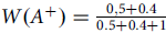 $W\left( {{A^ + }} \right){\rm{ }} = {{{0,5 + 0.4}}\over{{0.5 + 0.4 + 1}}}$
≈ 0.47, W(A
0) = 0,
$W\left( {{A^ + }} \right){\rm{ }} = {{{0,5 + 0.4}}\over{{0.5 + 0.4 + 1}}}$
≈ 0.47, W(A
0) = 0, $W\left( {{A^ - }} \right) = - {{\left| { - 0.5 - 0.5} \right|} \over {\left| { - 0.5 - 0.5} \right| + 1}}$
= −0.5, W(A
−−) = 0. Thus, W(A) ≈ 5.8 + 0.47 + 0 − 0.5 + 0 = 5.77. Next, let us assume that population B has the welfare vector w
B
= (0.5, 0.5, 0, −0.4, −0.5, −1, −2.3, −2.5). We then have: W(B
++) = 0,
$W\left( {{A^ - }} \right) = - {{\left| { - 0.5 - 0.5} \right|} \over {\left| { - 0.5 - 0.5} \right| + 1}}$
= −0.5, W(A
−−) = 0. Thus, W(A) ≈ 5.8 + 0.47 + 0 − 0.5 + 0 = 5.77. Next, let us assume that population B has the welfare vector w
B
= (0.5, 0.5, 0, −0.4, −0.5, −1, −2.3, −2.5). We then have: W(B
++) = 0, $W\left( {{B^ + }} \right) = {{0.5 + 0.5} \over {0.5 + 0.5 + 1}}$
= 0.5, W(B
0) = 0,
$W\left( {{B^ + }} \right) = {{0.5 + 0.5} \over {0.5 + 0.5 + 1}}$
= 0.5, W(B
0) = 0, $W\left( {{B^ - }} \right){\rm{ }} = - {{{\left| { - 0.5 - 0.4} \right|}}\over{{\left| { - 0.5 - 0.4} \right| + 1}}}$
≈ −0.47, W(B
−−) = −1 − 2.3 − 2.5 = −5.8. Thus, W(B) ≈ 0 + 0.5 + 0 − 0.47 − 5.8 = −5.77. Hence, A is better than B.
$W\left( {{B^ - }} \right){\rm{ }} = - {{{\left| { - 0.5 - 0.4} \right|}}\over{{\left| { - 0.5 - 0.4} \right| + 1}}}$
≈ −0.47, W(B
−−) = −1 − 2.3 − 2.5 = −5.8. Thus, W(B) ≈ 0 + 0.5 + 0 − 0.47 − 5.8 = −5.77. Hence, A is better than B.
Another example is the following: Population A has 10 000 000 000 people where each person has a welfare value of 10. Population Z has (unrealistically) 1 000 000 000 000 people where each person has a welfare value of 0.2. The social welfare of A is 100 000 000 000, but the social welfare of Z is just below 1. Thus, the five-stage measure avoids the repugnant conclusion.
6.2 The stairway measure
Someone might object to the first measure that it has misdiagnosed the mistake behind the repugnant conclusion. Although there is a distinction between significant and insignificant welfare values, the distinction is not due to a difference between high and low welfare stages, but rather due to a difference between clearly distinct welfare levels and small welfare variations. Distinct welfare levels contribute substantially to social welfare and small welfare variations contribute insubstantially. A consequence of this is that only people with high positive and low negative welfare contribute substantially to social welfare, since only high positive and low negative welfare are significantly different from the neutral level. Low positive and high negative welfare are just small variations of the neutral level.
In order to represent this idea more formally, we note that large welfare levels can be represented by integers and that small welfare variations can be represented by proper fractions (fractions that lie between −1 and 1). We then note that the lowest positive welfare values consist of just fractional values, whereas higher positive welfare values consist of integer values and (occasionally) remainder fractional values. For example: the low welfare value 0.4 consists only of the fractional component 4/10, whereas the higher welfare value 2.4 consists of a sum of the integer component 2 and the remainder fractional component 4/10. The two fractional values 4/10 are equally insignificant.
Next, we define a measure which aggregates significant (integer) and insignificant (fractional) welfare values differently. The measure may be called the fractional-value-dampened total measure, or more figuratively, the stairway measure. The last name is chosen because the measure represents the contribution of individual welfare to social welfare as analogous to a stairway, where the vertical risers represent significant levels of welfare, and the horizontal treads represent insignificant variations of welfare at the different levels. The measure aggregates significant integer values by summation, and insignificant fractional values by a function that assures that they cannot add up to more than 1, when aggregated across individuals. Again, aggregated insignificant values cannot trump significant values.
The above ideas can be defined more precisely as follows: let floor(x) be the largest integer ≤ x and ceil(x) be the smallest integer ≥ x. For positive numbers x, the integer part [x] = floor(x), whereas for negative numbers x, the integer part [x] = ceil(x). Each number x can then be expressed as the sum of two numbers, the integer part: [x], and the fractional part: x − [x]. Relative to the welfare value w(p i ) of a person p i , we denote the integer part of a positive welfare value by w Z+ (p i ) and the fractional part by w F+ (p i ), and we denote the integer part of a negative welfare value by w Z−(p i ) and the fractional part by w F−(p i ). For each population A, we then divide the members of A into three groups: A +, consisting of well-faring members p i + with welfare levels w(p i ) > 0; A 0, consisting of neutrally faring members p i 0 with welfare level w(p i ) = 0; and A −, consisting of ill-faring members p i − with welfare levels w(p i ) < 0.
Next, let W P be a measure of positive social welfare, W U a measure of neutral social welfare, W N a measure of negative social welfare, A a finite population, divided into A +, A 0 and A −, p a member of A, and w a measure of individual welfare. Let us assume that #A + = j and that #A − = k. The stairway measure W is then defined as follows: $\begin {align}W\left( A \right) &= {W_P}\left( {{A^ + }} \right) + {W_U}\left( {{A^0}} \right) + {W_N}\left( {{A^ - }} \right) \\&= {W_{PZ}}\left( {{A^ + }} \right) + {W_{PF}}\left( {{A^ + }} \right) + {W_U}\left( {{A^0}} \right) + {W_{NZ}}\left( {{A^ - }} \right) + {W_{NF}}\left( {{A^ - }} \right), \end{align}$
where ${W_{PZ}}\left( {{A^ + }} \right){\rm{ }} = \sum\limits_{i = 1}^j {{w_{Z + }}\left( {p_i^ + } \right)}, $ ${W_{PF}}\left( {{A^ + }} \right){\rm{ }} = {{{\sum\limits_{i = 1}^j {{w_{F + }}\left( {p_{_i}^ + } \right)} }}\over{{1 + \sum\limits_{i = 1}^j {{w_{F + }}\left( {p_{_i}^ + } \right)} }}},$ ${W_U}\left( {{A^0}} \right) = 0,$ ${W_{NF}}\left( {{A^ - }} \right){\rm{ }} = - {{{\sum\limits_{i = 1}^k {\left| {{w_{F - }}\left( {p_{_i}^ - } \right)} \right|} }}\over{{1 + \sum\limits_{i = 1}^k {\left| {{w_{F - }}\left( {p_{_i}^ - } \right)} \right|} }}},$ ${W_{NZ}}\left( {{A^ - }} \right){\rm{ }} = \sum\limits_{i = 1}^k {{w_{Z - }}\left( {{p_{_i}^ -}} \right)}.$
The stairway measure is discontinuous at each integer value for any individual welfare value in the individual welfare vector. Instead of contributing continuously to social welfare, individual welfare contributes discontinuously, in jumps. As was the case for the previous measure, the discontinuity becomes more pronounced, the larger the population. Social welfare makes a larger jump from (0.5, 0.5, 0.5) to (1, 1, 1) than it does from (0.5, 0.5) to (1, 1), for example (from 0.6 to 3 vs. from 0.5 to 2).
Let me give an example of how the measure works. First, let us assume that population A has the welfare vector w
A
= (2.5, 2.3, 1, 0.5, 0.4, 0, −0.5, −0.5). We then have W
PZ
(A
+) = 2 + 2 + 1 + 0 + 0 = 5, ${W_{PF}}\left( {{A^ + }} \right) = {{0.5 + 0.3 + 0,5 + 0.4} \over {0.5 + 0.3 + 0.5 + 0.4 + 1}}$
≈ 0.63, W
U
(A
0) = 0, W
NZ
(A
−) = 0 + 0 = 0,
${W_{PF}}\left( {{A^ + }} \right) = {{0.5 + 0.3 + 0,5 + 0.4} \over {0.5 + 0.3 + 0.5 + 0.4 + 1}}$
≈ 0.63, W
U
(A
0) = 0, W
NZ
(A
−) = 0 + 0 = 0, ${W_{NF}}\left( {{A^ - }} \right) = - {{\left| { - 0.5 - 0.5} \right|} \over {\left| { - 0.5 - 0.5} \right| + 1}}$
= −0.5. Thus, W(A) ≈ 5 + 0.63 + 0 − 0 − 0.5 = 5.13. Next, let us assume that population B has the welfare vector w
B
= (0.5, 0.5, 0, −0.4, −0.5, −1, −2.3, −2.5). We then have: W
PZ
(B
+) = 0 + 0 = 0,
${W_{NF}}\left( {{A^ - }} \right) = - {{\left| { - 0.5 - 0.5} \right|} \over {\left| { - 0.5 - 0.5} \right| + 1}}$
= −0.5. Thus, W(A) ≈ 5 + 0.63 + 0 − 0 − 0.5 = 5.13. Next, let us assume that population B has the welfare vector w
B
= (0.5, 0.5, 0, −0.4, −0.5, −1, −2.3, −2.5). We then have: W
PZ
(B
+) = 0 + 0 = 0, ${W_{PF}}\left( {{B^ + }} \right) = {{0.5 + 0.5} \over {0.5 + 0.5 + 1}}$
= 0.5, W
U
(B0) = 0, W
NZ
(B
−) = 0 − 0 − 1 − 2 − 2 = −5,
${W_{PF}}\left( {{B^ + }} \right) = {{0.5 + 0.5} \over {0.5 + 0.5 + 1}}$
= 0.5, W
U
(B0) = 0, W
NZ
(B
−) = 0 − 0 − 1 − 2 − 2 = −5, ${W_{NF}}\left( {{B^ - }} \right) = - {{\left| { - 0.4 - 0.5 - 0.3 - 0.5} \right|} \over {\left| { - 0.4 - 0.5 - 0.3 - 0.5} \right| + 1}}$
≈ −0.63. Thus, W(B) ≈ 0 + 0.5 + 0 − 5 − 0.63 = −5.13. Again, A is better than B.
${W_{NF}}\left( {{B^ - }} \right) = - {{\left| { - 0.4 - 0.5 - 0.3 - 0.5} \right|} \over {\left| { - 0.4 - 0.5 - 0.3 - 0.5} \right| + 1}}$
≈ −0.63. Thus, W(B) ≈ 0 + 0.5 + 0 − 5 − 0.63 = −5.13. Again, A is better than B.
The stairway measure avoids the repugnant conclusion in the same way as the five-stage measure, so the same example that was used there could be used here as well.
6.3 Variants of the hybrid measures
Having presented two hybrid social welfare measures, the question thus arises: Which one should we choose: the five-stage measure or the stairway measure? Well, I do not think that we should choose either of them, as they stand. The reason for this is that both hybrid measures are much too simple to be suitable as measures of social welfare. A plausible measure of social welfare should attach more importance to negative welfare than to positive welfare, I think. And a plausible measure of social welfare should also be responsive to equality of welfare, which neither the macro-functions nor the micro-functions are. These flaws could easily be remedied, however. For the macro-functions, we could replace the suggested total measure with a measure that puts a larger weight on illfare and rewards equality (such as a non-normalized version of the social welfare measure proposed in Enflo Reference Enflo2021). For the micro-functions, we could transform each individual welfare value by a concave function and add a weight to illfare. If we make these adjustments, we get two new hybrid measures which have several merits over the simpler ones. I will not discuss these merits here, however, but will rather focus on the merits (and problems) of the original measures. This is because I want to stay focused on the hybrid measures as possible solutions to the problem of the repugnant conclusions.
Even so, we might wonder which type of hybrid measure is preferable: a five-stage measure, which dampens values close to zero, or a stairway measure, which dampens proper fractions. Unfortunately, I do not have an answer to this question. A five-stage measure is simpler in the sense that it assumes only two additional contributive thresholds, besides those between positive, neutral and negative welfare. The cost of this simplicity is that it has to be motivated by some arguments for the theses that there are contributive thresholds between significant and insignificant welfare and that there are no more than two such thresholds (one for negative and one for positive welfare). A stairway measure is simpler in the sense that it assumes that the contributive thresholds follow a regular pattern, where significant and insignificant welfare values coincide with clearly distinct welfare levels and small welfare variations, conveniently represented by integers and fractions. The cost of this simplicity is that it has to be motivated by an argument for the thesis that the contribution of individual welfare to social welfare follows a similar pattern. It seems to me that a considered choice between the two types of measures cannot be made without a better understanding of how individual welfare is related to the significance of welfare (for individuals and, by extension, for social welfare). This understanding, in turn, requires a better understanding of individual welfare. And such an undertaking falls outside the scope of this paper.
7. Merits of the Hybrid Measures
A virtue of both hybrid measures is that they are based on a simple and common idea, that quantities can be either significant or insignificant, and that small quantities are intrinsically insignificant. Furthermore, the hybrid measures do what they are designed to do: avoid the repugnant conclusions. They will not rank a possible large population of very well-faring people below a larger possible population of barely well-faring people; neither will they rank a possible large population of very ill-faring people above a larger possible population of barely ill-faring people. This is because the large, good population will have a social welfare value above 1, whereas the larger good population will have a social welfare value below 1, and because the large, bad population will have a social welfare value below −1, whereas the larger bad population will have a social welfare value above −1.
Unlike typical lexical vector measures, both hybrid measures can be used in expected utility calculations, without ending up with the implausible conclusion that it would always be better to try to realize a population with high welfare values than a population with low welfare values. This is because the hybrid measures (unlike lexical vector measures) measure high and low welfare on the same scale. An expected value including a high positive welfare value with a low probability can therefore be smaller than an expected value including a low positive welfare value with a high probability.
Moreover, both hybrid measures satisfy the impartiality condition. This is because the measures assign the same values for populations with welfare vectors that are permutations of each other. Both measures also satisfy the dominance condition. This is because the macro-functions and the micro-functions satisfy the dominance condition separately, and also because higher welfare values always dominate lower welfare values, even when they are aggregated by different functions. Both hybrid measures satisfy both monotonicity conditions as well. This is because both the macro-functions and the micro-functions satisfy both monotonicity conditions separately.
The hybrid measures also avoid other undesirable conclusions. They avoid the reverse repugnant conclusion because they function just like the total measure for significant welfare values, so that a small population of extremely well-faring people cannot be ranked above a large population of very well-faring people. The measures also avoid the two sadistic conclusions. They avoid the sadistic conclusion because they satisfy both monotonicity conditions, which means that adding people with positive welfare always makes a population better, whereas adding people with negative welfare always makes a population worse. They avoid the strong sadistic conclusion because the social welfare value of populations with negative welfare will be a negative number, whereas the social welfare value of populations with positive welfare will be a positive number. In addition, they avoid the following well-known conclusion:
Very repugnant conclusion: For any possible population of people with very high (and equal) positive welfare, there is a possible population consisting of people with very low positive welfare and people with very low negative welfare that is higher ranked.Footnote 34
The hybrid measures avoid this conclusion because populations with very low positive welfare simply cannot compete with populations with very high positive welfare, since their social welfare will be less than 1.
8. Potential Problems for the Hybrid Measures
All of the above features of the hybrid measures are appealing. But let us also consider some potential problems for these types of measures.
8.1 Relative repugnance
One potential problem for the hybrid measures is that although the measures escape the original repugnant conclusion, they do not escape all variants of it. The repugnancy of the original conclusion can be regarded in two different ways. According to one view, the repugnant conclusion is repugnant because people in the larger population fare much worse than people in the smaller population. According to another view, the repugnant conclusion is repugnant because people in the larger population fare much worse than people in the smaller population and, in addition, they are barely well-faring.Footnote 35 The hybrid measures avoid repugnancy in accordance with the second view, but not in accordance with the first view. This is because it is only people with insignificant welfare whose social welfare cannot compete with the social welfare of people with significant welfare. When comparisons are made between populations where everyone has significant welfare, many people with worse significant welfare can compete with fewer people with better significant welfare. Likewise, when comparisons are made between populations where everyone has insignificant welfare, many people with worse insignificant welfare can compete with fewer people with better insignificant welfare.
For insignificant welfare, this does not seem like an important problem, because the insignificant welfare values are so small. For significant positive welfare, and with respect to the original repugnant conclusion, this also seems like an acceptable result. Without the assumption that people in the larger population are barely well-faring, the repugnant conclusion does not appear so repugnant. (Also, it is not clear what the maximal welfare level is for people, so it is not clear that there could be a large difference in welfare between people at different positive levels.Footnote 36 ) For significant negative welfare, and with respect to the negative repugnant conclusion, it might be less acceptable that it is only people with the highest negative welfare whose welfare contributions cannot compete with welfare contributions of people at lower levels. Here one could have the intuition that a large population of very ill-faring people just cannot be as bad as a smaller population of extremely ill-faring people. If this is the case, the hybrid measures would have to be redesigned. (One could, for example, redesign them so that values w < 1 never add up to more than 1, values 1 ≤ w < 2 never add up to more than 2, a.s.o. Such a measure would not avoid the reverse repugnant conclusion, however.)
8.2 Sharp thresholds
Another potential problem for the new measures is that they require that there is a sharp boundary between significant and insignificant welfare values. There are philosophers who have found this implausible, for various reasons.
A first possible objection is that although there is a distinction between significant and insignificant welfare, the distinction is not sharp, but imprecise.Footnote 37 This view takes seriously the intuition that we do not seem to know exactly where the threshold lies. It explains our lack of knowledge with the impossibility of knowledge. Metaphysically, imprecise thresholds seem strange, however. Imprecision seems to belong to our understanding of the world, rather than to the world itself. But we need not believe in metaphysical imprecision to adopt a measure based on imprecise thresholds. We could just embrace epistemic imprecision regarding where the thresholds lie. (After all, it is not strange that we do not know where the thresholds lie, considering that we barely know what welfare is.) In practice, this idea might be captured by using a probability function for different measurement values. I will not be able to develop such an idea here, however.
A second possible objection is that although there is a distinction between significant and insignificant welfare, there are no thresholds between them, because the properties are non-exclusive. All welfare values are both significant and insignificant to different degrees. A welfare value can be more or less significant than another, but it is not either significant or insignificant. Initially, this view might seem appealing, because it allows us to accept that welfare can be significant and insignificant, without accepting any threshold between the two. However, it is difficult to turn this view into a measure that avoids the repugnant conclusion. If significance is a matter of degree, it is natural to think that significance covaries with welfare, so that welfare values further from zero are more significant than welfare values that are closer. But this idea is difficult to represent. We cannot just measure social welfare by degrees of significance, because then the distinction between positive and negative welfare is lost. If we add this distinction, we get a measure that is equivalent to the total measure and implies the repugnant conclusion. If we instead use significance as a weight on welfare values, so that more significant values get a larger weight, we get something worse than the total measure, a measure that rewards inequality. There may be other representations to try, but the basic idea does not seem very promising in this context.
A third possible objection is that although there is a distinction between significant and insignificant welfare, the distinction pertains only to welfare differences and not to welfare values. There simply cannot be a distinction in significance between adjacent welfare values; such distinctions only belong to welfare values that are widely apart.Footnote 38 If this is correct, then we are in trouble, however. This idea cannot be represented by a transitive measure, so it is not suitable for measurement purposes.Footnote 39 Furthermore, the idea misses that small welfare values seem insignificant in themselves. A welfare value of 0.1 is insignificant because it is small, which is different to how a welfare value of 100 is insignificant in comparison to a welfare value of 10 000. It is repugnant that a population with people at 0.1 is ranked above a population of very well-faring people, because 0.1 is an insignificant amount of welfare, regardless of how much better the very well-faring people fare.Footnote 40
I think that there are several considerations that speak in favour of the idea that there are sharp thresholds between significant and insignificant welfare values. One relevant consideration is that almost everyone agrees that there are at least some sharp welfare thresholds, namely those between positive, neutral and negative welfare.Footnote 41 No one finds it counterintuitive that a population of a few slightly well-faring people is better than any population of neutrally faring people, for example. The thresholds between positive, neutral and negative welfare show that welfare values could be very similar in one way and still very dissimilar in another. A low positive welfare value (0.5) is as similar to a higher positive welfare value (1) as it is similar to a neutral welfare value (0), and it is as similar to an even higher positive welfare value (1.5) as it is similar to a negative welfare value (−0.5), in one sense of ‘similar’, considering the differences in value between the five welfare values. Yet people at the three positive levels have a positive effect on social welfare, whereas people at the neutral level have a neutral effect, and people at the negative level have a negative effect. The five welfare levels are thus also very dissimilar, in another sense of ‘similar’, considering their intrinsic properties and their effects on social welfare. None of this strikes us as odd, as we are used to these thresholds. The question is thus not whether there are contributive thresholds, but whether there are more thresholds than those between positive, neutral and negative welfare.
The best argument for there being thresholds between significant and insignificant welfare is perhaps that we do seem to distinguish between significant and insignificant welfare – this explains our reactions to the repugnant conclusion. And the best argument for these thresholds being sharp is perhaps that other ways of understanding the distinction seem needlessly complicated or are difficult to represent in a measure that avoids the repugnant conclusion.
8.3 Discontinuity
Another potential problem with the hybrid measures is that they are discontinuous measures. This means that there are some cases where a continuous variation of inputs (in terms of a vector of individual welfare values) does not result in a continuous variation of outputs (in terms of a social welfare value). The five-stage measure is discontinuous from below at 1 and from above at −1 for any individual welfare value in the vector of individual welfare values. The stairway measure is discontinuous at each integer value for any individual welfare value in the vector of individual welfare values. On both measures, a population of two people with welfare 0.99 gets a social welfare value of roughly 0.66, whereas a population of two people with welfare 1 gets a social welfare value of 2. Thus, a small variation in individual welfare results in a jump in social welfare.
The discontinuity of the hybrid measures implies that individual welfare changes of the same size can have very different effects, depending on the initial welfare of the people whose welfare is changed. For the five-stage measure, this might happen when the initial welfare is between −1 and 1, and the welfare change is smaller than 1. For the stairway measure, this might happen for any initial welfare level and any welfare change, as long as small value variations are involved. For example, a population of two people with welfare 0.99, raised by 0.1, gets a social welfare change of roughly 1.44, whereas a population of two people with welfare 0.5, raised by 0.1, gets a social welfare change of roughly 0.05, on both measures.
Some philosophers find the above examples to be convincing counterexamples against discontinuous measures. They find it counterintuitive that what seem like very similar inputs could result in very dissimilar outputs. In particular, they find it counterintuitive that values just below some threshold affect social welfare very differently than values at the threshold do. It is, for example, a common critique of discontinuous measures that they have the counterintuitive consequence that a population of just a few well-faring people is ranked as better than a population with a larger number of slightly worse-faring people.Footnote 42
However, I suspect that this result seems counterintuitive to these critics just because they already have an intuition that there simply cannot be a contributive threshold between two adjacent welfare values. A small increase or decrease in welfare just cannot make such a large difference as that between insignificant and significant welfare, they think. A possible reply to this worry is that, with respect to welfare changes having different effects depending on the initial welfare of the people whose welfare levels are changed, this happens in other cases too. Small and insignificant changes in some quantitative property can have large effects by adding (or removing) the remainder of what is needed for some other property to arise. In the welfare case, a small increase can make more of a difference to individual welfare as well as to social welfare, if it allows a person to go from negative welfare to neutral or positive welfare than if it does not contribute to such a change. Similarly, a small increase can make more of a difference to individual welfare as well as to social welfare, if it allows a person to go from insignificant to significant welfare.
8.4 Non-separability
Yet another potential problem with the hybrid measures is that they are non-separable measures, that is, the contribution of one person’s welfare value to social welfare is dependent on the contributions of other people. This is a consequence of the micro-functions of the hybrid measures dividing a welfare total with the same welfare total plus 1. For example, if we add a person p i with a welfare value of w(p i ) = 0.5 to population A with welfare vector w A = (0.4, 0.5, 0.3), this increases social welfare by roughly 0.08. However, if we add a person p i with the same welfare value to population B with welfare vector w B = (0.6, 0.5, 0.4), this increases social welfare by roughly 0.07. Thus, the contribution of an individual depends on the contribution of other individuals in the same population. Some philosophers have found this unintuitive and have proposed separability (or independence) as a necessary property for a social welfare measure.Footnote 43
Considered by itself, separability certainly seems like a desirable property for a social welfare measure. However, there are other considerations that make separability seem less indispensable. One such consideration is that it seems relevant for the goodness of populations how its members fare vis-à-vis each other, and if so, separability cannot hold. It is, for example, relevant whether the members fare equally well.
A critic might retort that it is possible to accommodate equality with a concave function, saving separability. And also, even if separability is dispensable due to interdependence between people mattering for social welfare, there is an issue with how separability is abandoned in the case of the hybrid measures, namely by assuming diminishing value contributions by individual welfare values. Thus, another potential problem with the hybrid measures is that they presuppose that some values have diminishing contributive value, as a total.
8.5 Diminishing value contribution
It seems intuitive that a certain quantity of welfare should have the same effect on social welfare, no matter its context.Footnote 44 However, this intuition puts us in a bit of a dilemma. The idea that welfare values have diminishing contributive value may not be intuitively appealing in itself. But in a context where we want to capture several other intuitions concerning social welfare, the idea seems more appealing than its alternatives. The assumption that a total of small welfare values has diminishing contributive value prevents insignificant values from trumping significant ones. It allows us to avoid the repugnant conclusion without sacrificing dominance and monotonicity. The only other options that have these properties, I believe, are lexical ones, and such options have other issues. I should also emphasize that the idea of diminishing contributive value is confined to a total of small welfare values. Since small values are not so important, the problem that their contribution diminishes should not be that important either.
8.6 Equality ignored
A final potential problem with the hybrid measures is that they do not always reward equality. We can adjust both hybrid measures so that they reward equality in the distribution of welfare values that have the same sort of significance. This could be done, for example, in the ways described in section 6.3. However, we cannot adjust the hybrid measures so that they reward equality across welfare values of different sorts of significance. For example: an equality adjusted five-stage measure rewards equality in comparisons between populations with welfare vectors such as (5, 5, 5) and (7.5, 5, 2.5); (0, 0, 0) and (1, 0, −1); (0.5, 0.5, 0.5) and (0.75, 0.5, 0.25); and even (0, 0, 0) and (0.1, 0, −0.1). But it will not reward equality in comparisons between populations with welfare vectors such as (0.5, 0.5, 0.5) and (1, 0.5, 0). Here, it will reward inequality and rank the second and unequal population over the first and equal population. The reason for this is that the second population has one person with significant welfare, one that is high enough to contribute substantially to social welfare. An equality-adjusted stairway measure will have the same implication, in this case. (It will also favour unequal populations with welfare vectors such as (3, 2.5, 2) over populations with welfare vectors such as (2.5, 2.5, 2.5).) So, even equality-adjusted hybrid measures do not satisfy egalitarian conditions such as Pigou–Dalton, Hammond’s equity and inequality aversion.Footnote 45
Is this failure to reward equality in all circumstances a terrible consequence of equality adjusted hybrid measures? One could argue that it is not. For one thing, equality-adjusted hybrid measures reward equality in almost all cases. For another thing, if there are contributive thresholds that make a significant difference to individuals, it might be better that a few people are above such a threshold than that everyone is below, even if they all fare equally.Footnote 46 It might be better that some people’s welfare increases enough to push them over a threshold, than that everyone’s welfare increases without making a significant difference to anyone. This might be the case even if the changes that push people over the threshold are smaller than the changes that do not. Thus, it might be better if one person at 0.9 gets 0.1 to rise up to 1 than if billions of people at 0.1 get 0.8 to rise up to 0.9. If this seems odd, do remember that these are all small changes! We are talking of insignificant levels of welfare here – jellybean joys and mosquito-bite miseries, and similar trifles.
Moreover, the idea that equality is not always preferable is precisely what stops the various versions of Parfit’s famous continuum arguments for the repugnant conclusion, where the conclusion that a very large population of barely well-faring people (Z) is better than a large population of very well-faring people (A) is reached by “improvements” on A. In one version, the improvements consist of welfare increases, additions of well-faring people and equalizations of welfare.Footnote 47 The hybrid measures block the repugnant conclusion because they do not treat equalization as better when everyone falls below significant welfare.
9. Measures Compared
Having considered the merits and potential problems of the new hybrid measures, it might be useful to compare them to the previously proposed measures that were considered in section 4, both in terms of their general characteristics and in terms of their merits and problems. I provide two comparative tables, below. The first table compares the measures by some of their characteristic properties, as well as their ability to satisfy various desiderata for a social welfare measure, apart from avoiding any unwanted conclusions. The second table compares the measures by their ability to avoid different kinds of unwanted conclusions. Some of the measures in the table are completely specified, whereas other measures are types with different possible representations. I have assumed the descriptions of the measures provided in section 4. At times, not all possible representations of a certain type of measure avoid some unwanted conclusion, but as long as some of them do, I have marked their type as a “yes”.
We may note that no measure has a “Yes” for all rows, across all columns. This is no coincidence. Philosophers have worked out several impossibility results that show that there are some desiderata that cannot be jointly satisfied by any social welfare measure.Footnote 48 Looking at the tables, we are looking at possibilities, and possibilities involve compromises, unfortunately.
10. Conclusion
In this paper, I have discussed ways in which social welfare measures could avoid the repugnant conclusion. I have suggested that in order to avoid the conclusion without getting into worse problems, it is important to correctly identify the mistaken assumption behind it. After rejecting several diagnoses of the mistake, I proposed that the mistaken assumption is that welfare values that are not significant for an individual, by being small, can be significant for social welfare, by being sufficiently many. A large population of barely well-faring people cannot be better than a smaller population of very well-faring people because small welfare values do not contribute to social welfare in the same substantial way as larger welfare values do. I introduced two social welfare measures that capture this idea: the five-stage measure and the stairway measure. Last, I discussed some merits and some potential flaws of the new measures. On the positive side, the new measures satisfy impartiality, dominance and strict monotonicity conditions and avoid a number of undesirable conclusions, including the repugnant, the negative repugnant, the reverse repugnant, the sadistic, the strong sadistic and the very repugnant conclusions. On the negative side, the new measures are non-separable, rely on diminishing value contributions, and do not universally reward equality.
Formal properties

Table 1. Long description
Table 1 compares the total measure, the average measure, capped-number measures, number-dampened measures, neutral-range measures, critical-level measures, leximin, lexical vector measures, diminishing-returns measures and hybrid measures. The table shows whether the measures have the formal properties of being scalar, non-hybrid, continuous, impartial and separable and satisfying dominance and positive and negative strict monotonicity conditions. All measures are scalar, except for leximin and lexical vector measures. All measures satisfy impartiality, except for diminishing-returns measures. All measures satisfy dominance, except for capped-number and neutral-range measures. The total measure has all of the eight formal properties. Critical-level measures have seven of the properties, but do not satisfy positive strict monotonicity. The average measure and number-dampened measures have five of the properties, but are non-separable and do not satisfy the two monotonicity conditions. Lexical vector measures have five of the properties, but are hybrid and discontinuous. Diminishing-returns measures have four of the properties, including satisfying the two monotonicity conditions. Neutral-range measures have three of the properties, including separability. Leximin has three of the properties, including being non-hybrid. Capped-number measures only have the two properties already mentioned (being scalar and impartial). The hybrid measures proposed in the paper have five of the properties, but are hybrid, discontinuous and non-separable.
Avoidance of unwanted conclusions

Table 2. Long description
Table 2 compares the total measure, the average measure, capped-number measures, number-dampened measures, neutral-range measures, critical-level measures, leximin, lexical vector measures, diminishing-returns measures and hybrid measures. The table shows whether the measures avoid the repugnant, negative repugnant, reverse repugnant, very repugnant, sadistic and strong sadistic conclusions. All measures, except for the total measure, avoid the repugnant and very repugnant conclusions. All measures, except for critical-level measures, avoid the strong sadistic conclusion. All measures, except for total and critical-level measures, avoid the negative repugnant conclusion. All measures, except for the average measure and leximin, avoid the reverse repugnant conclusion. All measures avoid the sadistic conclusion, except for the average, capped-number, number-dampened and critical -level measures. The hybrid measures avoid all six unwanted conclusions.
* Even though these measures avoid the unwanted conclusion stated in terms of “is better than”, they do not avoid a variant of the conclusion, stated in terms of “is equally valuable as”.
Acknowledgements
For invaluable help and encouragement, I am grateful to Per Enflo, Victor Moberger, Katie Steele and two anonymous referees.
Disclosure statement
I confirm that I have no conflict of interest.
Karin Enflo is Associate Professor in Philosophy at Umeå University. Her research has mainly focused on measurement of quantitative properties within different areas of science and philosophy, such as social welfare, freedom of choice, equality, similarity and diversity. Her work has appeared in journals such as Inquiry, Pacific Philosophical Quarterly, Social Choice and Welfare and Journal of Ethics and Social Philosophy. URL: https://www.umu.se/en/staff/karin-enflo/
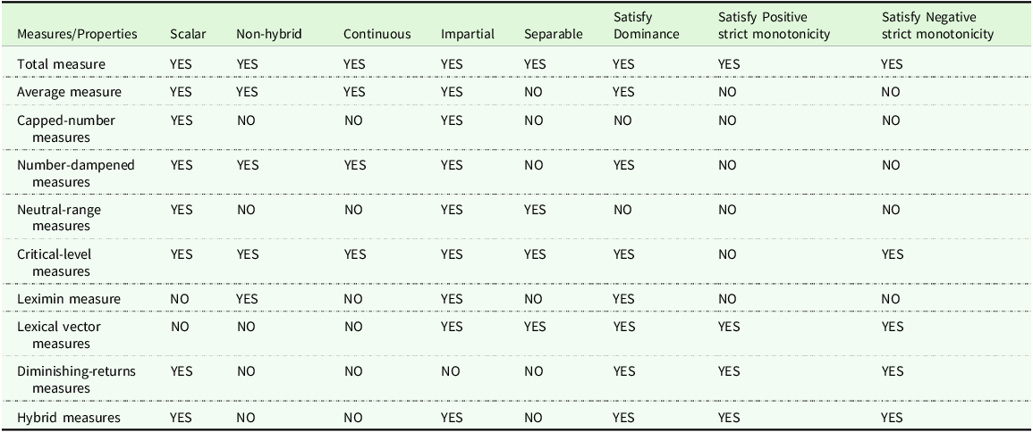
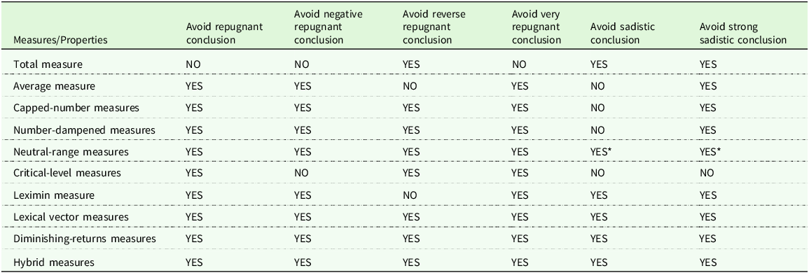

 Open access

