





1 Introduction
The theory of causal fermion systems is a recent approach to fundamental physics (for an introduction to the physical background and applications as well as the mathematical context, we refer the interested reader to the review [Reference Finster, Jokel, Finster, Giulini, Kleiner and Tolksdorf9], the textbooks [Reference Finster8, Reference Finster, Kindermann and Treude10] or the website [1]). In this approach, spacetime and all structures therein are encoded in a measure $\rho $
on a set of operators on a Hilbert space. The physical equations are formulated via a variational principle for the measure
$\rho $
on a set of operators on a Hilbert space. The physical equations are formulated via a variational principle for the measure $\rho $
, the so-called causal action principle. Causal variational principles evolved as a mathematical generalization of the causal action principle [Reference Finster7, Reference Finster and Kleiner11, Reference Finster and Langer12] (an introduction to the causal action principle and causal variational principles can be found for example in [Reference Finster, Kindermann and Treude10, Chapters 5 and 6]). From the point of view of the calculus of variations, causal variational principles are a class of nonlinear, nonconvex variational principles where one minimizes an action
$\rho $
, the so-called causal action principle. Causal variational principles evolved as a mathematical generalization of the causal action principle [Reference Finster7, Reference Finster and Kleiner11, Reference Finster and Langer12] (an introduction to the causal action principle and causal variational principles can be found for example in [Reference Finster, Kindermann and Treude10, Chapters 5 and 6]). From the point of view of the calculus of variations, causal variational principles are a class of nonlinear, nonconvex variational principles where one minimizes an action ${\mathcal {S}}$
under variations of a measure
${\mathcal {S}}$
under variations of a measure $\rho $
. One of the objectives of the present paper is to formulate and analyze corresponding flows of measures. Moving from the study of minimizing measures to flows of measures can be understood in analogy to the transition from stationary problems (like for example minimizing the Dirichlet energy) to corresponding evolution equations (like for example the heat flow). In simple terms, our flows can be understood as gradient flows corresponding to causal variational principles. Due to the lack of convexity and smoothness, the formulation of the flow equations as well as the proof of existence of solutions are mathematically challenging and seem of general interest in the context of nonsmooth and nonconvex variational problems.
$\rho $
. One of the objectives of the present paper is to formulate and analyze corresponding flows of measures. Moving from the study of minimizing measures to flows of measures can be understood in analogy to the transition from stationary problems (like for example minimizing the Dirichlet energy) to corresponding evolution equations (like for example the heat flow). In simple terms, our flows can be understood as gradient flows corresponding to causal variational principles. Due to the lack of convexity and smoothness, the formulation of the flow equations as well as the proof of existence of solutions are mathematically challenging and seem of general interest in the context of nonsmooth and nonconvex variational problems.
1.1 Causal variational principles
In order to describe this objective and underlying obstructions in more detail, we begin by recalling the general setting of causal variational principles. For simplicity, we firstly restrict attention to the so-called compact setting; the detailed set-up shall be deferred to Section 2.1 below.
Our starting point is a compact metric space $(\mathscr F, d)$
and a non-negative function
$(\mathscr F, d)$
and a non-negative function ${{\mathcal {L}}} : \mathscr F \times \mathscr F \rightarrow \mathbb R^+_0 := [0, \infty )$
(the Lagrangian) which is assumed to be continuous. The corresponding causal action principle then is to
${{\mathcal {L}}} : \mathscr F \times \mathscr F \rightarrow \mathbb R^+_0 := [0, \infty )$
(the Lagrangian) which is assumed to be continuous. The corresponding causal action principle then is to
 $$ \begin{align} \text{minimize}\quad {\mathcal{S}} (\rho) = \int_{\mathscr F} \operatorname{d}\! \rho(x) \int_{\mathscr F} \operatorname{d}\! \rho(y)\: {\mathcal{L}}(x,y) \end{align} $$
over the class $\mathfrak {M}_1(\mathscr F)$
of normalized Borel measures on
$\mathfrak {M}_1(\mathscr F)$
of normalized Borel measures on $\mathscr F$
. Causal variational principles are a class of examples for nonsmooth and nonconvex variational principles. The existence of solutions of (1.1) is a consequence of the direct method of the Calculus of Variations (see Section 2.1). Most importantly, minimizers
$\mathscr F$
. Causal variational principles are a class of examples for nonsmooth and nonconvex variational principles. The existence of solutions of (1.1) is a consequence of the direct method of the Calculus of Variations (see Section 2.1). Most importantly, minimizers $\rho $
satisfy the corresponding Euler-Lagrange equations (EL equations for brevity), and their precise formulation is given in Section 2.1.
$\rho $
satisfy the corresponding Euler-Lagrange equations (EL equations for brevity), and their precise formulation is given in Section 2.1.
Constructing solutions of the EL equations – or physically meaningful approximations thereof – is of central importance in the theory of causal fermion systems in order to get a better understanding of the nature of the physical interactions as described by the causal action principle. Here, abstract existence results are not sufficient, but one needs constructive methods which give insight into the structure of the minimizing measure. By the aforementioned lack of smoothness and nonconvexity, this is a nontrivial task in itself. In this regard, a central objective of the general theory is to find a canonical way of how a generic probability measure $\rho _{0}$
can be modified continuously to yield an (approximative) solution of the EL equations. In other words, this corresponds to a meaningful evolution
$\rho _{0}$
can be modified continuously to yield an (approximative) solution of the EL equations. In other words, this corresponds to a meaningful evolution $t\mapsto \varrho (t)$
with
$t\mapsto \varrho (t)$
with $\varrho (0)=\rho _{0}$
such that, for
$\varrho (0)=\rho _{0}$
such that, for $t\to \infty $
,
$t\to \infty $
, $\varrho (t)$
approaches an (approximative) solution of the EL equations.
$\varrho (t)$
approaches an (approximative) solution of the EL equations.
1.2 Gradient flows
By the variational nature of the problems considered here, it is natural to consider evolutions driven by the energies or actions given by (1.1). By this we mean that the energies of the solutions are decreasing in time. Heuristically, this can be interpreted as a measure-valued variant of the ordinary differential equation
 $$ \begin{align} \left\{ \begin{array}{rll} \displaystyle \frac{\operatorname{d}\!}{\operatorname{d}\! t} \varrho(t)&= - \nabla {\mathcal{S}}(\varrho) &\; \text{ if }~t>0\:, \\[0.5em] \varrho(0) &= \rho_{0}\:. \end{array} \right. \ \end{align} $$
However, for future reference, we remark that (1.2) has to be understood symbolically; in our case and as shall be discussed below, this is due to the lack of smoothness, in turn being a consequence of the nonconvexity and nonsmoothness of the action $\mathcal {S}$
.
$\mathcal {S}$
.
By way of comparison, in the more familiar situation of classical Dirichlet energies, for example, on Sobolev spaces, (1.2) reduces to the usual heat equation. The convexity of the underlying energies then allows for useful a priori estimates, finally leading to both existence and regularity assertions for the respective flows. These methods have been refined and extended to many other flow equations, provided that the driving energies are convex.
1.3 Flows for nonconvex variational problems
The situation changes drastically if the underlying energies are no longer convex. To the best of our knowledge, there is no unifying theory that yields both existence and decisive statements on the long-time behavior of solutions of the associated gradient flows (see however related results in [Reference Rossi and Savaré16, Reference Bellettini, Novaga and Paolini4, Reference Rossi, Segatti and Stefanelli17, Reference Muratori and Savaré15, Reference Streets18]). To overcome the first issue, we employ a version of De Giorgi’s minimizing movements approach [Reference De Giorgi6, Reference Ambrosio2, Reference Braides5, Reference Fleißner14] adapted to the present setting; in essence, they can be understood as a method for extending the gradient flow to nonsmooth actions on infinite-dimensional spaces. This construction leads to a flow
 $$ \begin{align*} \Phi : [0,\infty)\times\mathfrak{M}_1(\mathscr F) \to \mathfrak{M}_1(\mathscr F) \end{align*} $$
with the property that the action given by (1.1) is strictly decreasing along the flow lines. In essence, this is achieved by solving variational problems in discrete time steps which are penalized by the Wasserstein metric, and then pass to a continuous time evolution by use of an Arzelà-Ascoli-type argument. While we describe an analogous penalization procedure by use of the total variation norm, the use of the Wasserstein metric is most suitable here. Indeed, it is the weak*-convergence of probability measures for which compactness can be achieved and the actions (1.1) are lower semicontinuous; the Wasserstein metric, in turn, induces weak*-convergence. We also study the analogous procedure for the total variation norm. In this case, we also get existence of a flow. But the flow has the shortcoming that it potentially gets stuck away from local minima (as will be explained in an example in Section 5). With this in mind, it seems that the Wasserstein distance is the correct metric for the flow of measures we have in mind. We prove that the resulting curves of measures are Hölder continuous (see Section 4.3).
It is an important task to control the long-time behavior of solutions. It is here where the interplay of nonconvexity and the weak compactness properties of weak*-convergence necessitate additional arguments. First, it is clear from the arbitrariness of the initial value $\rho _{0}$
that, at best, the curve will converge to an extremal point but not necessarily to a minimizer. In fact, by the very definition of the flow, it might get stuck at a critical point of the functional, and by the nonconvexity, the latter might be far away from any global minimizer. In the general situation considered here, the situation is even worse: it may happen that the gradient flow does not converge at all. This will be shown in Section 3 in a simple example where the potential is constructed as a downward spiral with increasingly small potential wells (see Figure 1 on page 8). In examples of this type, which may be known to the experts in different scenarios, there is not even a subsequence of times
$\rho _{0}$
that, at best, the curve will converge to an extremal point but not necessarily to a minimizer. In fact, by the very definition of the flow, it might get stuck at a critical point of the functional, and by the nonconvexity, the latter might be far away from any global minimizer. In the general situation considered here, the situation is even worse: it may happen that the gradient flow does not converge at all. This will be shown in Section 3 in a simple example where the potential is constructed as a downward spiral with increasingly small potential wells (see Figure 1 on page 8). In examples of this type, which may be known to the experts in different scenarios, there is not even a subsequence of times $(t_{k})$
for which the measures converge to a solution of the EL equations.
$(t_{k})$
for which the measures converge to a solution of the EL equations.
In order to overcome such difficulties, we also introduce another flow which involves an additional penalization term involving a parameter $\xi>0$
. In the case
$\xi>0$
. In the case $\xi =0$
, we get back the above flow by minimizing movements. In the case
$\xi =0$
, we get back the above flow by minimizing movements. In the case $\xi>0$
, the additional penalization term gives us a priori control of the length of the curve (as measured in the Wasserstein distance) in terms of the change of the action (see Section 4.4). This makes it possible to reparametrize the curve, using the action itself as the new parameter. In this way, we can circumvent the difficulty that the flow might get stuck in “plateaus” of the potential for a long time (as shown in Figure 2 on page 20). After the reparametrization, the curve becomes even Lipschitz continuous (see Section 4.4). Moreover, we get control of the long-time behavior of the solutions. Indeed, in the case
$\xi>0$
, the additional penalization term gives us a priori control of the length of the curve (as measured in the Wasserstein distance) in terms of the change of the action (see Section 4.4). This makes it possible to reparametrize the curve, using the action itself as the new parameter. In this way, we can circumvent the difficulty that the flow might get stuck in “plateaus” of the potential for a long time (as shown in Figure 2 on page 20). After the reparametrization, the curve becomes even Lipschitz continuous (see Section 4.4). Moreover, we get control of the long-time behavior of the solutions. Indeed, in the case $\xi>0$
we prove that the resulting curve
$\xi>0$
we prove that the resulting curve $\varrho ^\xi (t)$
does converge (see Section 4.5). The prize to pay is that the limiting measure satisfies the EL equations only approximately. For the error term, we derive a precise a priori bound which tends to zero as
$\varrho ^\xi (t)$
does converge (see Section 4.5). The prize to pay is that the limiting measure satisfies the EL equations only approximately. For the error term, we derive a precise a priori bound which tends to zero as $\xi \searrow 0$
. With this in mind, our procedure seems well-suited for the applications in mind. For example, in a numerical study one can choose
$\xi \searrow 0$
. With this in mind, our procedure seems well-suited for the applications in mind. For example, in a numerical study one can choose $\xi $
so small that the error of the approximation is bounded by the numerical errors.
$\xi $
so small that the error of the approximation is bounded by the numerical errors.
We also extend our methods and results to the causal action principle for causal variational principles. Our methods and results can be understood more generally from the perspective of nonconvex variational problems. Indeed, causal variational principles are model examples of variational principles which, in general, are fully nonconvex. The methods to be developed in the present paper provide Hölder continuous flows of measures with these desired properties.
1.4 Structure of the paper
The paper is organized as follows. After the necessary preliminaries on causal variational principles and measure theory (Section 2), we discuss a simple example of a nonsmooth and nonconvex variational problem in two dimensions (Section 3). In Section 4 flows are developed starting from minimizing movements for causal variational principles in the compact setting. In Section 5 our results are illustrated by further examples. Section 6 is devoted to the adaptation and generalization of our methods and results to the causal action principle in finite dimensions; this section also includes a brief but self-contained introduction to causal fermion systems and the causal action principle. Finally, in Section 7 we give an outlook on how our flow could be used for the study of the EL equations for causal fermion systems in infinite dimensions.
2 Preliminaries
2.1 Causal variational principles in the compact setting
We let $(\mathscr F, d)$
be a compact metric space and suppose that the Lagrangian
$(\mathscr F, d)$
be a compact metric space and suppose that the Lagrangian ${\mathcal {L}}\colon \mathscr F\times \mathscr F\to \mathbb R_{0}^{+}$
satisfies the following assumptions:
${\mathcal {L}}\colon \mathscr F\times \mathscr F\to \mathbb R_{0}^{+}$
satisfies the following assumptions:
-
(A1) ${\mathcal {L}}$
is symmetric:
${\mathcal {L}}(x,y)={\mathcal {L}}(y,x)$
for all
$x,y\in \mathscr F$
.
${\mathcal {L}}$
is symmetric:
${\mathcal {L}}(x,y)={\mathcal {L}}(y,x)$
for all
$x,y\in \mathscr F$
. -
(A2)
${\mathcal {L}} \in \operatorname {C}^0(\mathscr F \times \mathscr F, \mathbb R^+_0)$
is continuous in both arguments.




The causal variational principle is to minimize the action ${\mathcal {S}}$
defined as the double integral over the Lagrangian
${\mathcal {S}}$
defined as the double integral over the Lagrangian
 $$ \begin{align} {\mathcal{S}} (\rho) = \int_{\mathscr F} \operatorname{d}\! \rho(x) \int_{\mathscr F} \operatorname{d}\! \rho(y)\: {\mathcal{L}}(x,y) \end{align} $$
under variations of the measure $\rho $
within the class of regular Borel measures, keeping the total volume
$\rho $
within the class of regular Borel measures, keeping the total volume $\rho (\mathscr F)$
fixed (volume constraint). By rescaling the measure, it is no loss of generality to consider normalized measures, that is,
$\rho (\mathscr F)$
fixed (volume constraint). By rescaling the measure, it is no loss of generality to consider normalized measures, that is,
 $$ \begin{align*} \rho(\mathscr F) = 1 \:. \end{align*} $$
The existence of minimizers follows from standard compactness arguments (see [Reference Finster7] or, in a slightly more general scenario, [Reference Finster and Langer12, Section 3.2] or [Reference Finster, Kindermann and Treude10, Chapter 12]); the method will also be revisited in Lemma 4.2 below.
Given a minimizing measure $\rho \in \mathfrak {M}_1(\mathscr F)$
, we introduce the underlying spacetime M as its support,
$\rho \in \mathfrak {M}_1(\mathscr F)$
, we introduce the underlying spacetime M as its support,
 $$ \begin{align*} M := \operatorname{\mathrm{supp}} \rho := \mathscr F\setminus\bigcup \big\{ U\subset \mathscr F\;\text{open}\colon\;\rho(U)=0 \big\} \:. \end{align*} $$
In [Reference Finster and Kleiner11, Lemma 2.3] it was shown that a minimizer satisfies the Euler-Lagrange (EL) equations, which state that the continuous function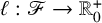 $\ell : \mathscr F \rightarrow \mathbb R_0^+$
defined by
$\ell : \mathscr F \rightarrow \mathbb R_0^+$
defined by
 $$ \begin{align*} \ell(x) := \int_{\mathscr F} {\mathcal{L}}(x,y)\: \operatorname{d}\! \rho(y) \end{align*} $$
is minimal on spacetime,
 $$ \begin{align} \ell|_{M} \equiv \inf_{\mathscr F} \ell \:. \end{align} $$
For further details we refer to [Reference Finster and Kleiner11, Section 2] or [Reference Finster, Kindermann and Treude10, Chapter 7]; we remark that we left out the parameter $\mathfrak {s}$
appearing in these contributions, which will not be required here.
$\mathfrak {s}$
appearing in these contributions, which will not be required here.
2.2 Background facts from optimal transport and metric measure spaces
We now fix our notation and recall a few background facts from measure theory and metric measure spaces to be used in the sequel. We specialize the setting by assuming that $\mathscr F$
is a compact metric space with metric d. We denote the set of probability measures on
$\mathscr F$
is a compact metric space with metric d. We denote the set of probability measures on $\mathscr F$
by
$\mathscr F$
by $\mathfrak {M}_{1}(\mathscr F)$
. More generally, we use
$\mathfrak {M}_{1}(\mathscr F)$
. More generally, we use $\mathfrak {M}(\mathscr F)$
to denote the signed Radon measures on
$\mathfrak {M}(\mathscr F)$
to denote the signed Radon measures on $\mathscr F$
and endow
$\mathscr F$
and endow $\mathfrak {M}(\mathscr F)$
with the total variation norm
$\mathfrak {M}(\mathscr F)$
with the total variation norm
 $$ \begin{align} \|\mu\|_{\mathfrak{M}(\mathscr F)} := \sup_{\pi\in\Pi(\mathscr F)}\sum_{B\in\pi}|\mu(B)|, \qquad \mu\in\mathfrak{M}(\mathscr F) \:, \end{align} $$
where $\Pi (\mathscr F)$
is the set of all countable Borel partitions of
$\Pi (\mathscr F)$
is the set of all countable Borel partitions of $\mathscr F$
. For future reference, we note that
$\mathscr F$
. For future reference, we note that $(\mathfrak {M}(\mathscr F), \|\mu \|_{\mathfrak {M}(\mathscr F)})$
is a Banach space, and that the metric induced by
$(\mathfrak {M}(\mathscr F), \|\mu \|_{\mathfrak {M}(\mathscr F)})$
is a Banach space, and that the metric induced by $\|\cdot \|_{\mathfrak {M}(\mathscr F)}$
, denoted by
$\|\cdot \|_{\mathfrak {M}(\mathscr F)}$
, denoted by $d_{\mathfrak {M}(\mathscr F)}$
, will also referred to as the Fréchet metric.
$d_{\mathfrak {M}(\mathscr F)}$
, will also referred to as the Fréchet metric.
In our arguments below, we will also make use of the p-Wasserstein metric on $\mathscr F$
for
$\mathscr F$
for $1 \leqslant p <\infty $
. Given a measure
$1 \leqslant p <\infty $
. Given a measure $\mathbb {P}\in \mathfrak {M}_{1}(\mathscr F \times \mathscr F)$
, for
$\mathbb {P}\in \mathfrak {M}_{1}(\mathscr F \times \mathscr F)$
, for $i\in \{1,2\}$
we denote the projection to the
$i\in \{1,2\}$
we denote the projection to the $i^{\text {th}}$
component by
$i^{\text {th}}$
component by $\pi ^{i}\colon \mathscr F \times \mathscr F \ni (x_{1},x_{2})\mapsto x_{i}\in \mathscr F$
. We let
$\pi ^{i}\colon \mathscr F \times \mathscr F \ni (x_{1},x_{2})\mapsto x_{i}\in \mathscr F$
. We let $\pi _{\#}^{i}\mathbb {P}(A):=\mathbb {P}(\pi _{i}^{-1}(A))$
for
$\pi _{\#}^{i}\mathbb {P}(A):=\mathbb {P}(\pi _{i}^{-1}(A))$
for $A \subset \mathscr F$
be the corresponding push-forward of
$A \subset \mathscr F$
be the corresponding push-forward of $\mathbb {P}$
. As is customary in this context, we then define for
$\mathbb {P}$
. As is customary in this context, we then define for $\mu _{1},\mu _{2}\in \mathfrak {M}_{1}(\mathscr F)$
the class of couplings
$\mu _{1},\mu _{2}\in \mathfrak {M}_{1}(\mathscr F)$
the class of couplings $\Gamma (\mu _{1},\mu _{2})$
(also referred to as transport plans) by
$\Gamma (\mu _{1},\mu _{2})$
(also referred to as transport plans) by
 $$ \begin{align*} \Gamma(\mu_{1},\mu_{2}) :=\{\mathbb{P}\in\mathfrak{M}_{1}(\mathscr F\times\mathscr F)\colon\; \pi_{\#}^{i}\mathbb{P}=\mu_{i}\;\text{for}\;i\in\{1,2\}\} \:. \end{align*} $$
Here the measures $\pi _{\#}^{i}\mathbb {P}$
are referred to as marginals. Let
$\pi _{\#}^{i}\mathbb {P}$
are referred to as marginals. Let $1\leqslant p<\infty $
. We then define for
$1\leqslant p<\infty $
. We then define for $\mu ,\nu \in \mathfrak {M}_{1}(\mathscr F)$
the p-th Wasserstein metric by
$\mu ,\nu \in \mathfrak {M}_{1}(\mathscr F)$
the p-th Wasserstein metric by
 $$ \begin{align} W_{p}(\mu,\nu) := \bigg( \inf\Big\{\int_{\mathscr F\times\mathscr F} d(x,y)^{p}\:\operatorname{d}\!\mathbb{P}(x,y)\;\colon \;\mathbb{P}\in\Gamma(\mu,\nu)\Big\} \bigg)^{\frac{1}{p}} \:. \end{align} $$
The integral appearing in (2.4) will also be abbreviated by $\mathbf {W}_{p}(\mathbb {P})$
. For future reference, let us emphasize that
$\mathbf {W}_{p}(\mathbb {P})$
. For future reference, let us emphasize that $W_{p}$
metrizes the weak*-convergence on
$W_{p}$
metrizes the weak*-convergence on $\mathfrak {M}_{1}(\mathscr F)$
, meaning that (see [Reference Villani19, Corollary 6.13])
$\mathfrak {M}_{1}(\mathscr F)$
, meaning that (see [Reference Villani19, Corollary 6.13])
 $$ \begin{align} \Big(\int_{\mathscr F}\varphi\operatorname{d}\!\mu_{j}\to \int_{\mathscr F}\varphi\operatorname{d}\!\mu\;\;\;\text{for all}\;\varphi\in \operatorname{C}(\mathscr F) \Big) \qquad \Longleftrightarrow \qquad W_{p}(\mu_{j},\mu)\to 0, \end{align} $$
where $\operatorname {C}(\mathscr F)$
denotes the continuous functions on
$\operatorname {C}(\mathscr F)$
denotes the continuous functions on $\mathscr F$
. The following lemma is clearly well-known to the experts, but since it is crucial for our arguments below, we include its short proof.
$\mathscr F$
. The following lemma is clearly well-known to the experts, but since it is crucial for our arguments below, we include its short proof.
Lemma 2.1. For any $p \in [1, \infty )$
the following inequality holds,
$p \in [1, \infty )$
the following inequality holds,
 $$ \begin{align} W_p(\mu, \nu) \leqslant \mathrm{{ diam }}(\mathscr F)\:\|\mu-\nu\|^{\frac{1}{p}}_{\mathfrak{M}(\mathscr F)} \qquad\text{for all}\;\mu,\nu\in\mathfrak{M}_{1}(\mathscr F) \:. \end{align} $$
Moreover, for any $\mu ,\nu \in \mathfrak {M}_{1}(\mathscr F)$
and
$\mu ,\nu \in \mathfrak {M}_{1}(\mathscr F)$
and $\lambda \in [0,1]$
,
$\lambda \in [0,1]$
,
 $$ \begin{align} W_{p} \big( \lambda\mu+(1-\lambda)\nu,\nu \big)\leqslant \lambda W_{p}(\mu,\nu). \end{align} $$
Proof. For the proof of (2.6) we introduce the measure
 $$ \begin{align*} \rho := \frac{1}{2}\: \big( \mu + \nu - |\mu-\nu| \big) \:. \end{align*} $$
Then the measures $\mu -\rho $
and
$\mu -\rho $
and $\nu - \rho $
are both positive, with total volume given by
$\nu - \rho $
are both positive, with total volume given by
 $$ \begin{align*} (\mu-\rho)(\mathscr F) = (\nu-\rho)(\mathscr F) = \frac{1}{2}\:\|\mu - \nu\|_{\mathfrak{M}(\mathscr F)} \:. \end{align*} $$
We consider the transport plan
 $$ \begin{align*} \mathbb{P}(x,y) := \rho(x) \: \delta(x,y) + \frac{2}{\|\mu - \nu\|_{\mathfrak{M}(\mathscr F)}}\:(\mu-\rho) \times (\nu-\rho) \:. \end{align*} $$
It has the desired marginals $\pi _{\#}^1 \mathbb {P}= \mu $
and
$\pi _{\#}^1 \mathbb {P}= \mu $
and $\pi _{\#}^2\mathbb {P}= \nu $
. We thus obtain the estimate
$\pi _{\#}^2\mathbb {P}= \nu $
. We thus obtain the estimate
 $$ \begin{align*} W_p(\mu, \nu)^p &\leqslant \iint_{\mathscr F \times \mathscr F} d(x,y)^p \: d \mathbb{P}(x,y) \\ &\leqslant \text{diam}(\mathscr F)^p\:\frac{2}{\|\mu - \nu\|_{\mathfrak{M}(\mathscr F)}}\:(\mu-\rho)(\mathscr F)\: (\nu-\rho)(\mathscr F) \\ &= \frac{1}{2}\:\text{diam}(\mathscr F)^p\:\|\mu-\nu\|_{\mathfrak{M}(\mathscr F)} \:. \end{align*} $$
This gives (2.6).
In order to prove (2.7), we let $\varepsilon>0$
be arbitrary and choose
$\varepsilon>0$
be arbitrary and choose $\mathbb {P}\in \Gamma (\mu ,\nu )$
,
$\mathbb {P}\in \Gamma (\mu ,\nu )$
, $\widetilde {\mathbb {P}}\in \Gamma (\nu ,\nu )$
such that
$\widetilde {\mathbb {P}}\in \Gamma (\nu ,\nu )$
such that
 $$ \begin{align} \mathbf{W}_{p}(\mathbb{P}) < W_{p}(\mu,\nu) + \varepsilon\quad\text{and}\quad \mathbf{W}_{p}(\widetilde{\mathbb{P}}) < \varepsilon. \end{align} $$
Now it suffices to realize that the coupling $\mathbb {P}':=\lambda \mathbb {P}+(1-\lambda )\widetilde {\mathbb {P}}$
has the two marginals
$\mathbb {P}':=\lambda \mathbb {P}+(1-\lambda )\widetilde {\mathbb {P}}$
has the two marginals
 $$ \begin{align*} \pi_{\#}^{1}\mathbb{P}'=\lambda\mu + (1-\lambda)\nu \qquad \text{and} \qquad \pi_{\#}^{2}\mathbb{P}'=\nu \:. \end{align*} $$
Hence $\mathbb {P}'\in \Gamma (\lambda \mu +(1-\lambda )\nu ,\nu )$
and therefore
$\mathbb {P}'\in \Gamma (\lambda \mu +(1-\lambda )\nu ,\nu )$
and therefore
 $$ \begin{align*} W_{p}(\lambda\mu+(1-\lambda)\nu,\nu) \leqslant \mathbf{W}_{p}(\mathbb{P}') & = \lambda \mathbf{W}_{p}(\mathbb{P}) + (1-\lambda)\mathbf{W}_{p}(\widetilde{\mathbb{P}}) \stackrel{(2.8)}{\leqslant} \lambda W_{p}(\mu,\nu)+ \varepsilon. \end{align*} $$
Sending $\varepsilon \searrow 0$
establishes (2.7), and this completes the proof.
$\varepsilon \searrow 0$
establishes (2.7), and this completes the proof.
Plot of the profile function ${\mathcal {S}}(r,0)$
.
${\mathcal {S}}(r,0)$
.

3 An example of a nonsmooth, nonconvex variational principle
In order to illustrate the familiar difficulties which one encounters when analyzing nonsmooth, nonconvex variational principles, we begin with an explicit example. Despite its simplicity, it has similar features as will be proven for general causal variational principles later on. In order to keep the setting as simple as possible, instead of varying on a space of measures, we consider a minimization problem for a function on $\mathbb R^2$
. We choose polar coordinates
$\mathbb R^2$
. We choose polar coordinates $(r, \varphi )$
and introduce the action
$(r, \varphi )$
and introduce the action ${\mathcal {S}}$
by
${\mathcal {S}}$
by
 $$ \begin{align*} {\mathcal{S}}(r, \varphi) = \left\{ \begin{array}{cl} \displaystyle 3 - 2 r^2 + r^2 \,(1-r^2)\: \sin \Big( \frac{1}{1-r} + \varphi \Big) &\qquad \text{ if }~r < 1 \\ \exp(1-r) &\qquad \text{if}~r \geq 1\:. \end{array} \right. \end{align*} $$
This action is smooth except on the unit circle $r=1$
, where it is merely continuous (see the radial plot in Figure 1).
$r=1$
, where it is merely continuous (see the radial plot in Figure 1).
Suppose that we want to find a minimizer using a gradient flow, that is,
 $$ \begin{align} \dot{\gamma}(t) = - \nabla {\mathcal{S}}|_{\gamma(t)} \qquad \text{and} \qquad \gamma(0) = \Big(r=\frac{1}{5}, \varphi=0 \Big) \:. \end{align} $$
Then the curve $\gamma (t)$
will “spiral outward” an infinite number of times. Therefore, it will not converge,
$\gamma (t)$
will “spiral outward” an infinite number of times. Therefore, it will not converge,
 $$ \begin{align*} \lim_{t \rightarrow \infty} \gamma(t) \qquad \text{does not exist}\:. \end{align*} $$
Instead, all the points of the unit circle are accumulation points of the curve. However, the points on the unit circle itself are not critical, because the action becomes smaller linearly if the radius is increased. This gradient flow can be realized using minimizing movements if one considers the action
 $$ \begin{align} {\mathcal{S}}(r, \varphi) + \frac{1}{2h}\: d\big( (r,\phi), (r',\phi') \big)^2 \:, \end{align} $$
where d denotes the Euclidean distance in $\mathbb R^2$
. Indeed, computing the first variation of this action in the Cartesian variables
$\mathbb R^2$
. Indeed, computing the first variation of this action in the Cartesian variables $x=r \cos \phi $
and
$x=r \cos \phi $
and $y=r \sin \phi $
, we obtain the EL equations
$y=r \sin \phi $
, we obtain the EL equations
 $$ \begin{align*} \begin{pmatrix} \partial_x {\mathcal{S}} \\ \partial_y {\mathcal{S}} \end{pmatrix} + \frac{1}{h} \: \begin{pmatrix} x-x' \\ y-y' \end{pmatrix} = 0 \:. \end{align*} $$
Assuming that the limit $h \searrow 0$
exists, we obtain the differential equation (3.1). Therefore, the penalized action (3.2) can be regarded as a discrete version of the gradient flow with step size h.
$h \searrow 0$
exists, we obtain the differential equation (3.1). Therefore, the penalized action (3.2) can be regarded as a discrete version of the gradient flow with step size h.
We next consider minimizing movements with an additional penalization term parametrized by $\xi>0$
,
$\xi>0$
,
 $$ \begin{align*} {\mathcal{S}}(r, \varphi) + \frac{1}{2h}\: d\big( (r,\phi), (r',\phi') \big)^2 + \xi\, d\big( (r,\phi), (r',\phi') \big)\:. \end{align*} $$
Now the corresponding flow equation takes the form
 $$ \begin{align*} \dot{\gamma}_\xi(t) = \left\{ \begin{array}{cl} \displaystyle - \frac{\|\nabla {\mathcal{S}}|_{\gamma(t)}\|- \xi}{\|\nabla {\mathcal{S}}|_{\gamma(t)}\|} \; \nabla {\mathcal{S}}|_{\gamma(t)} &\qquad \text{if }~\|\nabla {\mathcal{S}}|_{\gamma(t)}\| \geq \xi \\[1em] 0 &\qquad \text{otherwise}\:. \end{array} \right. \end{align*} $$
Therefore, the flow stops as soon as the norm of the gradient becomes smaller than $\xi $
. Choosing
$\xi $
. Choosing $\xi $
very small, the solution curve
$\xi $
very small, the solution curve $\gamma _\xi (t)$
will look similar to
$\gamma _\xi (t)$
will look similar to $\gamma (\tau )$
, but instead of “spiraling around” an infinite number of times, it will stop at a point near the unit circle. The resulting curve has finite length and a limit point,
$\gamma (\tau )$
, but instead of “spiraling around” an infinite number of times, it will stop at a point near the unit circle. The resulting curve has finite length and a limit point,
 $$ \begin{align*} \gamma_{\xi}(\infty) := \lim_{t \rightarrow \infty} \gamma_\xi(t) \qquad \text{exists} \:. \end{align*} $$
The drawback is that the EL equations are satisfied only approximately in the sense that
 $$ \begin{align*} \big\| \nabla {\mathcal{S}}|_{\gamma_\xi(\infty)} \big\| \leqslant \xi \:. \end{align*} $$
In the limit $\xi \searrow 0$
, the limit points
$\xi \searrow 0$
, the limit points $\gamma _\xi (\infty )$
again “spiral around” an infinite number of times. Therefore, the limit
$\gamma _\xi (\infty )$
again “spiral around” an infinite number of times. Therefore, the limit
 $$ \begin{align*} \lim_{\xi \searrow 0} \gamma_\xi(\infty) \qquad \text{does not exist}\:. \end{align*} $$
Instead, all the points of the unit circle are again accumulation points of the curve $\gamma _\xi (\infty )$
with
$\gamma _\xi (\infty )$
with $\xi \in \mathbb R^+$
.
$\xi \in \mathbb R^+$
.
4 Minimizing movements for causal variational principles
4.1 The causal action with penalization
Throughout this section, we tacitly suppose that Assumptions (A1) and (A2) on the Lagrangian hold. In order to set up the minimizing movements scheme, we first consider variational problems with a given penalization. In particular, given parameters $\xi \geq 0$
,
$\xi \geq 0$
, $h>0$
and a measure
$h>0$
and a measure $\rho $
, we define
$\rho $
, we define
 $$ \begin{align} {\mathcal{S}}^{h,\xi}(\mu):={\mathcal{S}}(\mu)+\frac{1}{2h}\: d(\mu,\rho)^2+ \xi\: d(\mu,\rho) \:, \end{align} $$
where d is the Fréchet or the Wasserstein distance, (cf. (2.3) and (2.4))
 $$ \begin{align} \text{Case~1.} \;\; d=d_{\mathfrak{M}(\mathscr F)} \qquad \text{or} \qquad \text{Case~2.} \;\; d = W_p \:. \end{align} $$
The existence of solutions of the underlying minimization problem will be proven in Lemma 4.2. We begin with the following preparatory result (for a similar weaker statement see [Reference Finster and Langer12, Theorem 3.4]).
Lemma 4.1. Let $(\mathscr F, d)$
be a compact metric space and let
$(\mathscr F, d)$
be a compact metric space and let ${\mathcal {L}}\in \operatorname {C}(\mathscr F\times \mathscr F)$
. Then the functional
${\mathcal {L}}\in \operatorname {C}(\mathscr F\times \mathscr F)$
. Then the functional
 $$ \begin{align*} {\mathcal{S}} \::\: \mathfrak{M}_{1}(\mathscr F)\ni\mu\mapsto \iint_{\mathscr F\times\mathscr F}{\mathcal{L}}(x,y)\operatorname{d}\!\mu(x)\operatorname{d}\!\mu(y) \end{align*} $$
is continuous with respect to weak*-convergence on $\mathfrak {M}_{1}(\mathscr F)$
.
$\mathfrak {M}_{1}(\mathscr F)$
.
Moreover, the functional ${\mathcal {S}}$
is Lipschitz continuous with respect to the Fréchet metric, that is, there is a constant C (which depends only on
${\mathcal {S}}$
is Lipschitz continuous with respect to the Fréchet metric, that is, there is a constant C (which depends only on $\mathscr F$
and
$\mathscr F$
and ${\mathcal {L}}$
) such that for all
${\mathcal {L}}$
) such that for all $\rho , \tilde {\rho } \in \mathfrak {M}_{1}(\mathscr F)$
,
$\rho , \tilde {\rho } \in \mathfrak {M}_{1}(\mathscr F)$
,
 $$ \begin{align} | {\mathcal{S}}(\tilde{\rho}) - {\mathcal{S}}(\rho) | \leqslant C\: d_{\mathfrak{M}(\mathscr F)}(\tilde{\rho}, \rho) \:. \end{align} $$
If we assume that the Lagrangian ${\mathcal {L}} \in \operatorname {C}^{0,\alpha }(\mathscr F \times \mathscr F, \mathbb R^+_0)$
is Hölder continuous with Hölder exponent
${\mathcal {L}} \in \operatorname {C}^{0,\alpha }(\mathscr F \times \mathscr F, \mathbb R^+_0)$
is Hölder continuous with Hölder exponent $\alpha \in (0,1]$
, then so is the functional
$\alpha \in (0,1]$
, then so is the functional ${\mathcal {S}}$
with respect to the Wasserstein distance, that is, there is a constant C (which again depends only on
${\mathcal {S}}$
with respect to the Wasserstein distance, that is, there is a constant C (which again depends only on $\mathscr F$
and
$\mathscr F$
and ${\mathcal {L}}$
) such that for all
${\mathcal {L}}$
) such that for all $\rho , \tilde {\rho } \in \mathfrak {M}_{1}(\mathscr F)$
,
$\rho , \tilde {\rho } \in \mathfrak {M}_{1}(\mathscr F)$
,
 $$ \begin{align} \big| {\mathcal{S}}(\tilde{\rho}) - {\mathcal{S}}(\rho) \big| \leqslant C\: W_p(\tilde{\rho}, \rho)^\alpha\:. \end{align} $$
Proof. Let $\rho ,\rho _{1},\rho _{2},...\in \mathfrak {M}_1(\mathscr F)$
be such that
$\rho ,\rho _{1},\rho _{2},...\in \mathfrak {M}_1(\mathscr F)$
be such that $\rho _{j}\stackrel {*}{\rightharpoonup }\rho $
as
$\rho _{j}\stackrel {*}{\rightharpoonup }\rho $
as $j\to \infty $
. Since
$j\to \infty $
. Since $\mathcal {F}$
is compact, the Weierstraß approximation theorem implies that the space
$\mathcal {F}$
is compact, the Weierstraß approximation theorem implies that the space
 $$ \begin{align*} X:=\mathrm{span}\{(x,y)\mapsto f(x)g(y)\colon\;f,g\in\operatorname{C}(\mathscr F)\} \end{align*} $$
is dense in $\operatorname {C}(\mathscr F \times \mathscr F)$
. Let
$\operatorname {C}(\mathscr F \times \mathscr F)$
. Let $\varepsilon>0$
be arbitrary but fixed. We then find
$\varepsilon>0$
be arbitrary but fixed. We then find $h\in \operatorname {C}(X \times X)$
of the form
$h\in \operatorname {C}(X \times X)$
of the form $h(x,y)=\sum _{i=1}^{N}h_{i}f_{i}(x)g_{i}(y)$
with
$h(x,y)=\sum _{i=1}^{N}h_{i}f_{i}(x)g_{i}(y)$
with $h_{1},...,h_{N}\in \mathbb R$
such that
$h_{1},...,h_{N}\in \mathbb R$
such that $\|{\mathcal {L}}-h\|_{\infty }<\varepsilon $
. Therefore,
$\|{\mathcal {L}}-h\|_{\infty }<\varepsilon $
. Therefore,
 $$ \begin{align*} &\left\vert \iint_{\mathscr F\times\mathscr F}{\mathcal{L}}(x,y)\operatorname{d}\!\rho(x)\operatorname{d}\!\rho(y) - \iint_{\mathscr F\times\mathscr F}{\mathcal{L}}(x,y)\operatorname{d}\!\rho_{j}(x)\operatorname{d}\!\rho_{j}(y)\right\vert \\ & \leqslant \iint_{\mathscr F\times\mathscr F}|{\mathcal{L}}(x,y)-h(x,y)|\operatorname{d}\!\rho(x)\operatorname{d}\!\rho(y) \\ & \quad\:+ \left\vert \iint_{\mathscr F\times\mathscr F}h(x,y) \operatorname{d}\!\rho_{j}(x) \operatorname{d}\!\rho_{j}(y) - \iint_{\mathscr F\times\mathscr F}h(x,y) \operatorname{d}\!\rho(x) \operatorname{d}\!\rho(y) \right\vert \\ & \quad\:+ \iint_{\mathscr F\times\mathscr F}|{\mathcal{L}}(x,y)-h(x,y)|\operatorname{d}\!\rho_{j}(x)\operatorname{d}\!\rho_{j}(y) =: \mathrm{I}+\mathrm{II}+\mathrm{III}. \end{align*} $$
We then have $\mathrm {I} \leqslant \varepsilon \rho (\mathscr F)^{2}$
and
$\mathrm {I} \leqslant \varepsilon \rho (\mathscr F)^{2}$
and $\mathrm {III}\leqslant \varepsilon m^{2}$
. On the other hand, by the very structure of h, the weak*-convergence
$\mathrm {III}\leqslant \varepsilon m^{2}$
. On the other hand, by the very structure of h, the weak*-convergence $\rho _{j}\stackrel {*}{\rightharpoonup }\rho $
implies
$\rho _{j}\stackrel {*}{\rightharpoonup }\rho $
implies
 $$ \begin{align*} \iint_{\mathscr F\times\mathscr F}h(x,y)\operatorname{d}\!\rho_{j}(x)\operatorname{d}\!\rho_{j}(y) & = \sum_{i=1}^{N}h_{i}\Big(\int_{\mathscr F}f(x)\operatorname{d}\!\rho_{j}(x) \Big)\Big(\int_{\mathscr F}g(y)\operatorname{d}\!\rho_{j}(y) \Big) \\ & \to \sum_{i=1}^{N}h_{i}\Big(\int_{\mathscr F}f(x)\operatorname{d}\!\rho(x) \Big)\Big(\int_{\mathscr F}g(y)\operatorname{d}\!\rho(y) \Big)\\ & = \iint_{\mathscr F\times\mathscr F}h(x,y)\operatorname{d}\!\rho(x)\operatorname{d}\!\rho(y) \end{align*} $$
as $j\to \infty $
, so that
$j\to \infty $
, so that $\mathrm {II}\to 0$
as
$\mathrm {II}\to 0$
as $j\to \infty $
. By arbitrariness of
$j\to \infty $
. By arbitrariness of $\varepsilon>0$
, the proof of continuity is complete.
$\varepsilon>0$
, the proof of continuity is complete.
In order to prove the Lipschitz bound (4.3), we rewrite the difference of the actions as
 $$ \begin{align*} &{\mathcal{S}} \big( \tilde{\rho} \big) - {\mathcal{S}} \big( \rho \big) = \int_{\mathscr F} \operatorname{d}\! \tilde{\rho}(x) \int_{\mathscr F} \operatorname{d}\! \tilde{\rho}(y)\: {\mathcal{L}}(x,y) - \int_{\mathscr F} \operatorname{d}\! \rho(x) \int_{\mathscr F} \operatorname{d}\! \rho(y)\: {\mathcal{L}}(x,y) \\ &= \int_{\mathscr F} \operatorname{d}\! \tilde{\rho}(x) \int_{\mathscr F} \operatorname{d}\! \big( \tilde{\rho}- \rho \big)(y) \: {\mathcal{L}}(x,y) + \int_{\mathscr F} \operatorname{d}\! \big(\tilde{\rho}- \rho\big)(x) \int_{\mathscr F} \operatorname{d}\! \rho(y)\: {\mathcal{L}}(x,y) \:. \end{align*} $$
Using that the Lagrangian is uniformly bounded and that the measures are normalized, we obtain the estimate,
 $$ \begin{align*} {\mathcal{S}} ( \tilde{\rho} ) - {\mathcal{S}} ( \rho ) \leqslant 2\,\|{\mathcal{L}}\|_{\operatorname{C}^0(\mathscr F \times \mathscr F)}\: d_{\mathfrak{M}(\mathscr F)}(\tilde{\rho}, \rho) \:, \end{align*} $$
proving (4.3).
In order to derive the Hölder estimate (4.4), we let $\nu \in \mathfrak {M}_1(\mathscr F \times \mathscr F)$
be a coupling of
$\nu \in \mathfrak {M}_1(\mathscr F \times \mathscr F)$
be a coupling of $\rho $
and
$\rho $
and $\tilde {\rho }$
. Then, using that the two marginals of
$\tilde {\rho }$
. Then, using that the two marginals of $\nu $
coincide with
$\nu $
coincide with $\rho $
and
$\rho $
and $\tilde {\rho }$
, the difference of actions can be written as
$\tilde {\rho }$
, the difference of actions can be written as
 $$ \begin{align*} {\mathcal{S}}(\tilde{\rho}) - {\mathcal{S}}(\rho) = \int_{\mathscr F \times \mathscr F} \operatorname{d}\! \nu(x,x') \int_{\mathscr F \times \mathscr F} \operatorname{d}\! \nu(y,y') \big( {\mathcal{L}}(x',y') - {\mathcal{L}}(x,y) \big) \:. \end{align*} $$
Using that the Lagrangian is Hölder continuous with Hölder constant denoted by c, we know that
 $$ \begin{align*} \big| {\mathcal{L}}(x',y') - {\mathcal{L}}(x,y) \big| & \leqslant \big| {\mathcal{L}}(x',y') -{\mathcal{L}}(x,y') \big| + \big| {\mathcal{L}}(x,y') - {\mathcal{L}}(x,y) \big| \\ & \leqslant c\: \big( d(x,x')^\alpha + d(y,y')^\alpha \big) \:. \end{align*} $$
We thus obtain
 $$ \begin{align*} \big| {\mathcal{S}}(\tilde{\rho}) - {\mathcal{S}}(\rho) \big| &\leqslant 2 c\: \int_{\mathscr F \times \mathscr F} d(x,x')^\alpha \: \operatorname{d}\! \nu(x,x') \leqslant 2c \:\bigg( \int_{\mathscr F \times \mathscr F} d(x,x')^p \: \operatorname{d}\! \nu(x,x') \bigg)^{\frac{\alpha}{p}}, \end{align*} $$
where in the last step we applied the Hölder inequality for normalized measures. Taking the infimum over all couplings gives the result.
Lemma 4.2. For any $\xi \geq 0$
,
$\xi \geq 0$
, $h>0$
and
$h>0$
and $\rho \in \mathfrak {M}_{1}(\mathscr F)$
, there exists a minimizer
$\rho \in \mathfrak {M}_{1}(\mathscr F)$
, there exists a minimizer $\mu \in \mathfrak {M}_{1}(\mathscr F)$
of the causal action with penalization (4.1).
$\mu \in \mathfrak {M}_{1}(\mathscr F)$
of the causal action with penalization (4.1).
Proof. Since ${\mathcal {L}}\colon \mathscr F\times \mathscr F\to \mathbb R_{0}^{+}$
,
${\mathcal {L}}\colon \mathscr F\times \mathscr F\to \mathbb R_{0}^{+}$
, $\mathcal {S}^{h,\xi }$
is bounded below on
$\mathcal {S}^{h,\xi }$
is bounded below on $\mathfrak {M}_{1}(\mathscr F)$
and thus
$\mathfrak {M}_{1}(\mathscr F)$
and thus $m:=\inf _{\mathfrak {M}_{1}(\mathscr F)}\mathcal {S}^{h,\xi }$
exists in
$m:=\inf _{\mathfrak {M}_{1}(\mathscr F)}\mathcal {S}^{h,\xi }$
exists in $[0,\infty )$
, we can choose a minimizing sequence
$[0,\infty )$
, we can choose a minimizing sequence $(\mu _{j})\subset \mathfrak {M}_{1}(\mathscr F)$
for
$(\mu _{j})\subset \mathfrak {M}_{1}(\mathscr F)$
for $\mathcal {S}^{h,\xi }$
, so that in particular
$\mathcal {S}^{h,\xi }$
, so that in particular $m=\lim _{j\to \infty }\mathcal {S}^{h,\xi }(\mu _{j})$
. By the duality relation
$m=\lim _{j\to \infty }\mathcal {S}^{h,\xi }(\mu _{j})$
. By the duality relation $\operatorname {C}_{0}(\mathscr F)'\cong \mathfrak {M}(\mathscr F)$
and using that
$\operatorname {C}_{0}(\mathscr F)'\cong \mathfrak {M}(\mathscr F)$
and using that $\mathfrak {M}_{1}(\mathscr F)$
is convex and closed, the Banach-Alaoglu theorem provides us with a nonrelabeled subsequence and a probability measure
$\mathfrak {M}_{1}(\mathscr F)$
is convex and closed, the Banach-Alaoglu theorem provides us with a nonrelabeled subsequence and a probability measure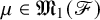 $\mu \in \mathfrak {M}_{1}(\mathscr F)$
such that we have
$\mu \in \mathfrak {M}_{1}(\mathscr F)$
such that we have $\mu _{j}\stackrel {*}{\rightharpoonup }\mu $
in
$\mu _{j}\stackrel {*}{\rightharpoonup }\mu $
in $\mathfrak {M}_{1}(\mathscr F)$
. By Lemma 4.1,
$\mathfrak {M}_{1}(\mathscr F)$
. By Lemma 4.1, $\mathcal {S}$
is continuous with respect to weak*-convergence. Now, if (i) d is the Fréchet metric, then
$\mathcal {S}$
is continuous with respect to weak*-convergence. Now, if (i) d is the Fréchet metric, then $d(\cdot ,\rho )=\|\cdot -\rho \|_{\mathfrak {M}(\mathscr F)}$
is lower semicontinuous with respect to weak*-convergence. On the other hand, if (ii) d is the p-Wasserstein metric, then d metrizes weak*-convergence and so, in particular,
$d(\cdot ,\rho )=\|\cdot -\rho \|_{\mathfrak {M}(\mathscr F)}$
is lower semicontinuous with respect to weak*-convergence. On the other hand, if (ii) d is the p-Wasserstein metric, then d metrizes weak*-convergence and so, in particular, $d(\cdot ,\rho )$
is continuous with respect to weak*-convergence. In both cases,
$d(\cdot ,\rho )$
is continuous with respect to weak*-convergence. In both cases, ${\mathcal {S}}^{h,\xi }$
is lower semicontinuous with respect to weak*-convergence. Hence,
${\mathcal {S}}^{h,\xi }$
is lower semicontinuous with respect to weak*-convergence. Hence,
 $$ \begin{align*} m \leqslant {\mathcal{S}}^{h,\xi}(\mu)\leqslant \liminf_{j\to\infty}{\mathcal{S}}^{h,\xi}(\mu_{j}) = m \:, \end{align*} $$
and therefore $\mu $
is a minimizer.
$\mu $
is a minimizer.
For clarity, we point out that minimizers will in general not be unique. Moreover, whereas the Fréchet metric $d_{\mathfrak {M}(\mathscr F)}$
might seem as an easier or more natural choice, it comes with unfavorable properties of the flow (see Section 5) which can be avoided by working with the Wasserstein distance
$d_{\mathfrak {M}(\mathscr F)}$
might seem as an easier or more natural choice, it comes with unfavorable properties of the flow (see Section 5) which can be avoided by working with the Wasserstein distance $W_{p}$
.
$W_{p}$
.
4.2 Minimizing movements
Let $\rho _{0}\in \mathfrak {M}_{1}(\mathcal {F})$
be a given initial measure. Throughout, we fix a penalization parameter
$\rho _{0}\in \mathfrak {M}_{1}(\mathcal {F})$
be a given initial measure. Throughout, we fix a penalization parameter $\xi \geq 0$
and, given
$\xi \geq 0$
and, given $h>0$
, consider the sequence of measures
$h>0$
, consider the sequence of measures $(\rho ^{h, \xi }_j)_{j \in \mathbb N_0}$
obtained by choosing
$(\rho ^{h, \xi }_j)_{j \in \mathbb N_0}$
obtained by choosing $\rho ^{h, \xi }_{j=0}=\rho _0$
and by iteratively minimizing the associated functional
$\rho ^{h, \xi }_{j=0}=\rho _0$
and by iteratively minimizing the associated functional
 $$ \begin{align} {\mathcal{S}}_{j}^{h,\xi}(\mu):={\mathcal{S}}(\mu)+\frac{1}{2h}\: d \big(\mu,\rho_{j-1}^{h,\xi} \big)^2+ \xi\: d(\mu,\rho_{j-1}^{h,\xi}) \end{align} $$
for $j=1,2,\ldots $
. The first penalization term follows the general procedure in the minimizing movements approach (see for example [Reference Ambrosio2]); also the resulting Hölder estimates (as in Lemma 4.5 and Proposition 4.6) are adaptations of standard arguments to our setting (see for example [Reference Braides5, Proposition 7.1]). The second penalization term in (4.5), however, is novel. The necessity of introducing this additional penalization term depending on
$j=1,2,\ldots $
. The first penalization term follows the general procedure in the minimizing movements approach (see for example [Reference Ambrosio2]); also the resulting Hölder estimates (as in Lemma 4.5 and Proposition 4.6) are adaptations of standard arguments to our setting (see for example [Reference Braides5, Proposition 7.1]). The second penalization term in (4.5), however, is novel. The necessity of introducing this additional penalization term depending on $\xi $
will be explained in detail in Section 4.4.
$\xi $
will be explained in detail in Section 4.4.
We begin by collecting several elementary estimates, where d is again the distance function induced by either the Fréchet metric or the Wasserstein distance (4.2):
Lemma 4.3. The sequence $(\rho ^{h, \xi }_j)_{j \in \mathbb N_0}$
satisfies for all
$(\rho ^{h, \xi }_j)_{j \in \mathbb N_0}$
satisfies for all $j \in \mathbb N$
the inequalities
$j \in \mathbb N$
the inequalities
 $$ \begin{align} \!{\mathcal{S}}(\rho_{j}^{h,\xi}) &\leqslant {\mathcal{S}} \big( \rho_{j-1}^{h,\xi} \big)\qquad\qquad\quad \end{align} $$
 $$ \begin{align} \!\!d \big( \rho_{j}^{h,\xi},\rho_{j-1}^{h,\xi} \big) &\leqslant \frac{1}{\xi} \: \Big( {\mathcal{S}} \big( \rho_{j-1}^{h,\xi} \big) - {\mathcal{S}} \big( \rho_{j}^{h,\xi} \big) \Big)\quad \end{align} $$
 $$ \begin{align} d \big( \rho_{j}^{h,\xi},\rho_{j-1}^{h,\xi} \big) &\leqslant \sqrt{ 2 h\, \big( {\mathcal{S}}(\rho_{j-1}^{h,\xi})-{\mathcal{S}}(\rho_{j}^{h,\xi}) \big) } \:. \end{align} $$
Moreover, the inequality (4.6) is strict unless $\rho _{j}^{h,\xi } = \rho _{j-1}^{h,\xi }$
.
$\rho _{j}^{h,\xi } = \rho _{j-1}^{h,\xi }$
.
Proof. The minimality implies that
 $$ \begin{align*} {\mathcal{S}}(\rho_{j}^{h,\xi})+\frac{1}{2h}d(\rho_{j}^{h,\xi},\rho_{j-1}^{h,\xi})^2 + \xi \:d(\rho_{j}^{h,\xi},\rho_{j-1}^{h,\xi}) & = {\mathcal{S}}_{j}^{h,\xi}(\rho_{j}^{h,\xi}) \\ &\leqslant {\mathcal{S}}_{j}^{h,\xi}(\rho_{j-1}^{h,\xi}) = {\mathcal{S}}(\rho_{j-1}^{h,\xi}) \:. \end{align*} $$
Using that the terms on the left are all non-negative, the result follows immediately.
4.3 A Hölder continuous flow
Our goal is to show that, taking a suitable limit $h \rightarrow 0$
, we to obtain a Hölder continuous curve
$h \rightarrow 0$
, we to obtain a Hölder continuous curve $\varrho ^\xi (t)$
with
$\varrho ^\xi (t)$
with $t \in \mathbb R^+_0$
. In preparation, we form the continuous curve
$t \in \mathbb R^+_0$
. In preparation, we form the continuous curve $\rho ^{h, \xi }$
by interpolation,
$\rho ^{h, \xi }$
by interpolation,
 $$ \begin{align} \rho^{h, \xi}(t) := \bigg( \Big\lfloor \frac{t}{h}+1\Big\rfloor -\frac{t}{h} \bigg)\:\rho_{\lfloor\frac{t}{h}\rfloor}^{h,\xi} + \bigg( \frac{t}{h} - \Big\lfloor \frac{t}{h} \Big\rfloor \bigg) \: \rho_{\lfloor\frac{t}{h}+1\rfloor}^{h,\xi} \:. \end{align} $$
For the next construction steps, we need the following generalization of the usual Arzelà-Ascoli theorem:
Lemma 4.4 [Reference Ambrosio, Gigli and Savaré3, Prop. 3.3.1]
Let $(X,d)$
be a complete metric space and
$(X,d)$
be a complete metric space and $T>0$
. Given a subset
$T>0$
. Given a subset $K\subset X$
which is sequentially compact with respect to a topology
$K\subset X$
which is sequentially compact with respect to a topology $\tau $
, suppose that
$\tau $
, suppose that $(u_{j})_{j\in \mathbb {N}}$
is a sequence of maps
$(u_{j})_{j\in \mathbb {N}}$
is a sequence of maps $u_{j}\colon [0,T]\to X$
such that
$u_{j}\colon [0,T]\to X$
such that
 $$ \begin{align} &\qquad u_{j}(t)\in K\qquad\text{for all}\;j\in\mathbb{N}\;\text{and all}\;t\in [0,T], \end{align} $$
 $$ \begin{align} & \limsup_{j\to\infty} d \big( u_{j}(s),u_{j}(t) \big)\leqslant \omega(s,t)\qquad\text{for all}\;s,t\in [0,T] \:, \end{align} $$
where $\omega \colon [0,T]\times [0,T]\to [0,\infty )$
is a symmetric function (i.e.,
$\omega \colon [0,T]\times [0,T]\to [0,\infty )$
is a symmetric function (i.e., $\omega (s,t)=\omega (t,s)$
for all
$\omega (s,t)=\omega (t,s)$
for all $s,t\in [0,T]$
) with the property that
$s,t\in [0,T]$
) with the property that $\lim _{(s,t)\to (0,0)}\omega (s,t)=0$
. Then there exists a subsequence
$\lim _{(s,t)\to (0,0)}\omega (s,t)=0$
. Then there exists a subsequence $(u_{j(k)})_{k\in \mathbb {N}}\subset (u_{j})_{j\in \mathbb {N}}$
and a d-continuous map
$(u_{j(k)})_{k\in \mathbb {N}}\subset (u_{j})_{j\in \mathbb {N}}$
and a d-continuous map $u\colon [0,T]\to X$
such that the sequence
$u\colon [0,T]\to X$
such that the sequence $(u_{j(k)})$
converges pointwise to u with respect to the topology
$(u_{j(k)})$
converges pointwise to u with respect to the topology $\tau $
.
$\tau $
.
Its applicability in the present framework follows from the following lemma:
Lemma 4.5. The curve $\rho ^{h, \xi }(t)$
defined by (4.9) satisfies for all
$\rho ^{h, \xi }(t)$
defined by (4.9) satisfies for all $0<t_{1},t_{2}<\infty $
the inequality
$0<t_{1},t_{2}<\infty $
the inequality
 $$ \begin{align} d \big( \rho^{h, \xi}(t_{1}),\rho^{h, \xi}(t_{2}) \big)\leqslant \sqrt{2}\: \sqrt{|t_{2}-t_{1}|+h}\; \sqrt{{\mathcal{S}}(\rho_{0})} \:. \end{align} $$
Proof. It clearly suffices to consider the case $t_{1}<t_{2}$
. Then, by definition of
$t_{1}<t_{2}$
. Then, by definition of $\rho _{h,\xi }$
,
$\rho _{h,\xi }$
,
 $$ \begin{align*} &d \big( \rho^{h, \xi}(t_{1}),\rho^{h, \xi}(t_{2}) \big) \leqslant d \Big( \big( \lfloor\tfrac{t_{1}}{h}+1\rfloor -\tfrac{t_{1}}{h} \big)\: \rho_{\lfloor\frac{t_{1}}{h} \rfloor}^{h,\xi} + \big( \tfrac{t_{1}}{h}-\lfloor\tfrac{t_{1}}{h}\rfloor \big) \: \rho_{\lfloor\frac{t_{1}}{h}+1\rfloor}^{h,\xi},\;\rho_{\lfloor\frac{t_{1}}{h}+1\rfloor}^{h,\xi} \Big) \\ &\;\; + d \Big( \rho_{\lfloor\frac{t_{2}}{h}\rfloor}^{h,\xi},\; \big( \lfloor\tfrac{t_{2}}{h}+1\rfloor -\tfrac{t_{2}}{h} \big)\: \rho_{\lfloor\frac{t_{2}}{h}\rfloor}^{h,\xi} + \big( \tfrac{t_{2}}{h}-\lfloor\tfrac{t_{2}}{h}\rfloor \big)\: \rho_{\lfloor\frac{t_{2}}{h}+1\rfloor}^{h,\xi} \Big) + \!\!\!\!\sum_{j=\lfloor\frac{t_{1}}{h}+1\rfloor}^{\lfloor\frac{t_{2}}{h}\rfloor -1}\!\!\! d\big( \rho_{j}^{h,\xi},\rho_{j+1}^{h,\xi} \big) \\ & \leqslant \Big( \lfloor\tfrac{t_{1}}{h}+1\rfloor -\tfrac{t_{1}}{h} \Big)\: d\big(\rho_{\lfloor\frac{t_{1}}{h}\rfloor}^{h,\xi},\: \rho_{\lfloor\frac{t_{1}}{h}+1\rfloor}^{h,\xi} \big) + \Big( \tfrac{t_{2}}{h}-\lfloor\tfrac{t_{2}}{h}\rfloor \Big)\: d \big( \rho_{\lfloor\frac{t_{2}}{h}\rfloor}^{h,\xi},\rho_{\lfloor\frac{t_{2}}{h}+1\rfloor}^{h,\xi} \big) \\ &\qquad \qquad + \sum_{j=\lfloor\frac{t_{1}}{h}+1\rfloor}^{\lfloor\frac{t_{2}}{h}\rfloor -1} d \big( \rho_{j}^{h,\xi},\rho_{j+1}^{h,\xi} \big) \:, \end{align*} $$
where the last step is trivial for d being the Fréchet metric and follows from Lemma 2.1 in the case of the Wasserstein metric. It follows that
 $$ \begin{align*} &d \big( \rho^{h, \xi}(t_{1}),\rho^{h, \xi}(t_{2}) \big) \leqslant \sum_{j=\lfloor\frac{t_{1}}{h}\rfloor}^{\lfloor\frac{t_{2}}{h}+1\rfloor -1}d(\rho_{j}^{h,\xi},\rho_{j+1}^{h,\xi}) \\ &\!\!\overset{(4.8)}{\leqslant} \sum_{j=\lfloor\frac{t_{1}}{h}\rfloor}^{\lfloor\frac{t_{2}}{h}+1\rfloor -1} \sqrt{ 2h\: \big( {\mathcal{S}}(\rho_{j}^{h,\xi})-{\mathcal{S}}(\rho_{j+1}^{h,\xi}) \big) }\\ & \leqslant \bigg( \sum_{j=\lfloor\frac{t_{1}}{h}\rfloor}^{\lfloor\frac{t_{2}}{h}+1\rfloor -1}1\bigg)^{\frac{1}{2}}\bigg(\sum_{j=\lfloor\frac{t_{1}}{h}\rfloor}^{\lfloor\frac{t_{2}}{h}+1\rfloor -1} 2h \:\big({\mathcal{S}}(\rho_{j}^{h,\xi})-{\mathcal{S}}(\rho_{j+1}^{h,\xi}) \big) \bigg)^{\frac{1}{2}} \:. \end{align*} $$
The last sum is telescopic. Moreover, using that the sequence of actions is monotone decreasing (4.6) and non-negative, we conclude that
 $$ \begin{align*} d \big( \rho^{h, \xi}(t_{1}),\rho^{h, \xi}(t_{2}) \big) \leqslant \sqrt{2} \: \sqrt{ (t_{2}-t_{1})+h} \: \sqrt{{\mathcal{S}}(\rho_{0})} \:. \end{align*} $$
This completes the proof.
We are now ready for proving our first existence result.
Proposition 4.6. For any $\xi \geq 0$
, there is a Hölder continuous flow
$\xi \geq 0$
, there is a Hölder continuous flow
 $$ \begin{align*} \varrho^\xi \in\operatorname{C}^{0,\frac{1}{2}} \big( [0,\infty), (\mathfrak{M}_1(\mathscr F),d) \big) \end{align*} $$
with $\varrho (0)=\rho _{0}$
. Setting
$\varrho (0)=\rho _{0}$
. Setting
 $$ \begin{align*} t_{\max} := \inf \big\{ t \in \mathbb R^+ \:\big|\: {\mathcal{S}}\big( \varrho^\xi(t) \big) = \inf_{\tau \in \mathbb R^+} {\mathcal{S}} \big( \varrho^\xi(\tau) \big) \big\} \;\in\; \mathbb R^+ \cup \{\infty\} \:, \end{align*} $$
the action is strictly monotone decreasing up to $t_{\max }$
, that is,
$t_{\max }$
, that is,
 $$ \begin{align} {\mathcal{S}}\big( \varrho^\xi(t_1) \big)> {\mathcal{S}}\big( \varrho^\xi(t_2) \big) \qquad \qquad \text{for all }~0 \leqslant t_1 < t_2 \leqslant t_{\max}\:. \end{align} $$
Moreover, the flow curve satisfies for all $0 \leqslant t_1 < t_2$
the Hölder bound
$0 \leqslant t_1 < t_2$
the Hölder bound
 $$ \begin{align*} d \big( \varrho^{\xi}(t_{1}),\varrho^{\xi}(t_{2}) \big)\leqslant \sqrt{2}\: \sqrt{t_{2}-t_{1}}\; \sqrt{{\mathcal{S}}(\rho_{0})} \:. \end{align*} $$
Proof.
Case 1. $d=W_{p}$
. Let
$d=W_{p}$
. Let $[T_{1},T_{2}]\subset [0,\infty )$
be a compact interval. We note that
$[T_{1},T_{2}]\subset [0,\infty )$
be a compact interval. We note that $(\mathfrak {M}_{1}(\mathscr F),W_{p})$
is a compact, hence complete, metric space by the Banach-Alaoglu theorem. We aim to apply Lemma 4.4 to the sequence
$(\mathfrak {M}_{1}(\mathscr F),W_{p})$
is a compact, hence complete, metric space by the Banach-Alaoglu theorem. We aim to apply Lemma 4.4 to the sequence $(\rho ^{\xi , 1/j})_{j\in \mathbb {N}}$
together with
$(\rho ^{\xi , 1/j})_{j\in \mathbb {N}}$
together with $d=W_{p}$
and
$d=W_{p}$
and $\tau $
being the weak*-topology on
$\tau $
being the weak*-topology on $\mathfrak {M}_{1}(\mathscr F)$
. Then
$\mathfrak {M}_{1}(\mathscr F)$
. Then $\rho ^{\xi , 1/j}(t)\in K:=\mathfrak {M}_{1}(\mathscr F)$
for all
$\rho ^{\xi , 1/j}(t)\in K:=\mathfrak {M}_{1}(\mathscr F)$
for all $j\in \mathbb {N}$
, whereby (4.10) is satisfied. Moreover, the estimate (4.12) yields that (4.11) is fulfilled with
$j\in \mathbb {N}$
, whereby (4.10) is satisfied. Moreover, the estimate (4.12) yields that (4.11) is fulfilled with $\omega (s,t):=\sqrt {2|s-t|}$
. Consequently, Lemma 4.4 together with (2.5) gives the existence of a
$\omega (s,t):=\sqrt {2|s-t|}$
. Consequently, Lemma 4.4 together with (2.5) gives the existence of a $W_{p}$
-continuous limit map
$W_{p}$
-continuous limit map $\rho ^{\xi }\colon [T_{1},T_{2}]\to \mathfrak {M}_{1}(\mathscr F)$
such that
$\rho ^{\xi }\colon [T_{1},T_{2}]\to \mathfrak {M}_{1}(\mathscr F)$
such that $\rho ^{\xi , 1/j(k)}(t) \to \varrho ^{\xi }(t)$
with respect to
$\rho ^{\xi , 1/j(k)}(t) \to \varrho ^{\xi }(t)$
with respect to $d=W_{p}$
for every
$d=W_{p}$
for every $t \in [T_{1},T_{2}]$
. For all
$t \in [T_{1},T_{2}]$
. For all $T_{1}\leqslant t_{1}\leqslant t_{2}\leqslant T_{2}$
we thus obtain
$T_{1}\leqslant t_{1}\leqslant t_{2}\leqslant T_{2}$
we thus obtain
 $$ \begin{align*} W_{p}(\varrho^{\xi}(t_{1}),\varrho^{\xi}(t_{2})) & \leqslant \limsup_{k\to\infty}(W_{p} ( \varrho^{\xi}(t_{1}),\rho^{\xi, 1/j(k)}(t_{1}) )+W_{p} ( \rho^{\xi, 1/j(k)}(t_{1}),\rho^{\xi, 1/j(k)}(t_{2}) ). \\ & \qquad\qquad\qquad +W_{p} ( \rho^{\xi, 1/j(k)}(t_{2}),\varrho^{\xi}(t_{2}) ) ) \leqslant \sqrt{2}\: \sqrt{t_{2}-t_{1}}\; \sqrt{{\mathcal{S}}(\rho_{0})} \end{align*} $$
by everywhere convergence and the estimate (4.12).
In order to construct the requisite curve as claimed in Proposition 4.6, we cover $[0,\infty )$
by intervals
$[0,\infty )$
by intervals $I_{\ell }:=[\ell -1,\ell +1]$
,
$I_{\ell }:=[\ell -1,\ell +1]$
, $\ell \in \mathbb {N}$
. By what has been said above, we may choose a sequence
$\ell \in \mathbb {N}$
. By what has been said above, we may choose a sequence $(j_{k}^{(1)})$
such that, for a certain limit curve
$(j_{k}^{(1)})$
such that, for a certain limit curve $\varrho ^{\xi }\in \operatorname {C}^{0,1/2}([0,2];\mathfrak {M}_{1}(\mathscr F))$
we have
$\varrho ^{\xi }\in \operatorname {C}^{0,1/2}([0,2];\mathfrak {M}_{1}(\mathscr F))$
we have
 $$ \begin{align*} \rho^{\xi, 1/j_k^{(1)}}\to\varrho^{\xi} \end{align*} $$
with respect to $W_{p}$
on
$W_{p}$
on $[0,2]$
as
$[0,2]$
as $k\to \infty $
. Next choose a subsequence
$k\to \infty $
. Next choose a subsequence $(j_{k}^{(2)})\subset (j_{k}^{(1)})$
such that
$(j_{k}^{(2)})\subset (j_{k}^{(1)})$
such that
 $$ \begin{align*} \rho^{\xi, 1/j_{k}^{(2)}} \to\overline{\varrho}^{\xi} \end{align*} $$
for a certain limit curve $\overline {\varrho }^{\xi }\in \operatorname {C}^{0,1/2}([1,3];\mathfrak {M}_{1}(\mathscr F))$
. Clearly, since
$\overline {\varrho }^{\xi }\in \operatorname {C}^{0,1/2}([1,3];\mathfrak {M}_{1}(\mathscr F))$
. Clearly, since $(h_{k}^{2})\subset (h_{k}^{1})$
, we must have
$(h_{k}^{2})\subset (h_{k}^{1})$
, we must have $\varrho =\overline {\varrho }$
on
$\varrho =\overline {\varrho }$
on $[1,2]$
, and then define
$[1,2]$
, and then define $\varrho ^{\xi }:=\overline {\varrho }^{\xi }$
on
$\varrho ^{\xi }:=\overline {\varrho }^{\xi }$
on $[2,3]$
. Proceeding iteratively in this way and passing to the diagonal sequence, we obtain a sequence
$[2,3]$
. Proceeding iteratively in this way and passing to the diagonal sequence, we obtain a sequence $(j_{l})$
with
$(j_{l})$
with $j_{l}\to \infty $
and a curve
$j_{l}\to \infty $
and a curve $\varrho ^{\xi }\in \operatorname {C}([0,\infty );(\mathfrak {M}_{1}(\mathscr F),W_{p}))\cap \operatorname {C}^{0,1/2}([0,\infty );(\mathfrak {M}_{1}(\mathscr F),W_{p}))$
such that for any compact subset
$\varrho ^{\xi }\in \operatorname {C}([0,\infty );(\mathfrak {M}_{1}(\mathscr F),W_{p}))\cap \operatorname {C}^{0,1/2}([0,\infty );(\mathfrak {M}_{1}(\mathscr F),W_{p}))$
such that for any compact subset $I\subset [0,\infty )$
there holds
$I\subset [0,\infty )$
there holds
 $$ \begin{align*} \rho^{\xi, 1/j_{l}}(t)\to \varrho(t)\;\;\text{for all }~t\in I \text{ in }~(\mathfrak{M}_{1}(\mathscr F),W_{p}) \:. \end{align*} $$
Case 2. $d=d_{\mathfrak {M}(\mathscr F)}$
. In this situation, we let
$d=d_{\mathfrak {M}(\mathscr F)}$
. In this situation, we let $d=d_{\mathfrak {M}(\mathscr F)}$
and again let
$d=d_{\mathfrak {M}(\mathscr F)}$
and again let $\tau $
be the weak*-topology on
$\tau $
be the weak*-topology on $\mathfrak {M}_{1}(\mathscr F)$
. Then
$\mathfrak {M}_{1}(\mathscr F)$
. Then $K:=\mathfrak {M}_{1}(\mathscr F)$
is compact for
$K:=\mathfrak {M}_{1}(\mathscr F)$
is compact for $\tau $
. Arguing as above, specifically applying (4.12) to
$\tau $
. Arguing as above, specifically applying (4.12) to $d=d_{\mathfrak {M}(\mathscr F)}$
, we obtain the existence of a limit map
$d=d_{\mathfrak {M}(\mathscr F)}$
, we obtain the existence of a limit map $\varrho ^{\xi } \in \operatorname {C}([0,\infty );(\mathfrak {M}_{1}(\mathscr F);d_{\mathfrak {M}(\mathscr F)}))$
such that, for some sequence
$\varrho ^{\xi } \in \operatorname {C}([0,\infty );(\mathfrak {M}_{1}(\mathscr F);d_{\mathfrak {M}(\mathscr F)}))$
such that, for some sequence $(j_{l})$
with
$(j_{l})$
with $j_{l}\to \infty $
as
$j_{l}\to \infty $
as $l\to \infty $
,
$l\to \infty $
, $\rho ^{\xi , 1/j_{l}}\to \varrho $
in
$\rho ^{\xi , 1/j_{l}}\to \varrho $
in $(\mathfrak {M}_{1}(\mathscr F),W_{p})$
(not in
$(\mathfrak {M}_{1}(\mathscr F),W_{p})$
(not in $(\mathfrak {M}_{1}(\mathscr F),d_{\mathfrak {M}(\mathscr F)})$
), locally uniformly in time (i.e., uniformly in t in a compact subset of
$(\mathfrak {M}_{1}(\mathscr F),d_{\mathfrak {M}(\mathscr F)})$
), locally uniformly in time (i.e., uniformly in t in a compact subset of $[0, \infty )$
).
$[0, \infty )$
).
Let us note that we have $\varrho ^{\xi }\in \operatorname {C}_{\operatorname {loc}}^{0,1/2}([0,\infty );(\mathfrak {M}_{1}(\mathscr F),d_{\mathfrak {M}(\mathscr F)}))$
indeed: Let
$\varrho ^{\xi }\in \operatorname {C}_{\operatorname {loc}}^{0,1/2}([0,\infty );(\mathfrak {M}_{1}(\mathscr F),d_{\mathfrak {M}(\mathscr F)}))$
indeed: Let $0\leqslant T_{1}\leqslant T_{2}<\infty $
, so that
$0\leqslant T_{1}\leqslant T_{2}<\infty $
, so that $\rho ^{\xi , 1/j_{l}}(t)\stackrel {*}{\rightharpoonup }\varrho ^{\xi }(t)$
for all
$\rho ^{\xi , 1/j_{l}}(t)\stackrel {*}{\rightharpoonup }\varrho ^{\xi }(t)$
for all $t\in [T_{1},T_{2}]$
since
$t\in [T_{1},T_{2}]$
since $W_{p}$
metrizes weak*-convergence on
$W_{p}$
metrizes weak*-convergence on $\mathfrak {M}(\mathscr F)$
. Since in the present setting (4.12) is available for
$\mathfrak {M}(\mathscr F)$
. Since in the present setting (4.12) is available for $d=d_{\mathfrak {M}(\mathscr F)}$
, we conclude for
$d=d_{\mathfrak {M}(\mathscr F)}$
, we conclude for $t, t' \in [T_{1},T_{2}]$
by weak*-lower semicontinuity of the total variation norm
$t, t' \in [T_{1},T_{2}]$
by weak*-lower semicontinuity of the total variation norm
 $$ \begin{align*} \|\varrho^{\xi}(t)-\varrho^{\xi}(t')\|_{\mathfrak{M}(\mathscr F)} & \leqslant \liminf_{l\to\infty} \|\varrho_{1/j_{l}}^{\xi}(t)-\varrho_{1/j_{l}}^{\xi}(t') \|_{\mathfrak{M}(\mathscr F)} \stackrel{(4.12)}{\leqslant} \sqrt{2 {\mathcal{S}}(\rho_0)}\: |t-t'|^{\frac{1}{2}} \:. \end{align*} $$
In this sense, the passage to the weak*-metric is only required to obtain the existence of such a curve, whereas the Hölder regularity for $d_{\mathfrak {M}(\mathscr F)}$
survives from Lemma 4.5 by lower semicontinuity. This concludes the proof of Proposition 4.6.
$d_{\mathfrak {M}(\mathscr F)}$
survives from Lemma 4.5 by lower semicontinuity. This concludes the proof of Proposition 4.6.
Note that the previous theorem holds both in the case of the Wasserstein metric and the Fréchet metric on $\mathfrak {M}_{1}(\mathscr F)$
. However, the flow in these two cases has quite different properties, as will be illustrated in Section 5 by a few examples.
$\mathfrak {M}_{1}(\mathscr F)$
. However, the flow in these two cases has quite different properties, as will be illustrated in Section 5 by a few examples.
4.4 A Lipschitz curve in the case
$\xi>0$

The introduction of a positive penalization parameter $\xi>0$
in (4.5) is motivated by the fact that it gives us curves of finite length in
$\xi>0$
in (4.5) is motivated by the fact that it gives us curves of finite length in $\mathfrak {M}(\mathscr F)$
. In order to see this, we iterate (4.7) and use again that
$\mathfrak {M}(\mathscr F)$
. In order to see this, we iterate (4.7) and use again that ${{\mathcal {S}}}$
is monotone decreasing. We thus obtain
${{\mathcal {S}}}$
is monotone decreasing. We thus obtain
 $$ \begin{align} \sum_{j={n+1}}^N d \big( \rho_j^{h,\xi},\rho_{j-1}^{h,\xi} \big) \leqslant \frac{1}{\xi} \:\big( {\mathcal{S}}(\rho_n^{h,\xi})-{\mathcal{S}}(\rho_N^{h,\xi}) \big)\:, \end{align} $$
showing that the length of the discrete curve is bounded by the total change of the action. This estimate suggests that it is useful to use the action itself for the parametrization of the curve. As we shall see, it is of advantage to do so already for the discrete curve, before taking the limit $h \searrow 0$
(as will be explained in Remark 4.13 below). To this end, given
$h \searrow 0$
(as will be explained in Remark 4.13 below). To this end, given $h,\xi>0$
, we set
$h,\xi>0$
, we set
 $$ \begin{align} s_j = {\mathcal{S}} \big( \rho^{h, \xi}_j \big) \qquad \text{with }~j \in \mathbb N \:. \end{align} $$
Then the sequence $(s_j)_{j \in \mathbb N}$
is monotone decreasing,
$(s_j)_{j \in \mathbb N}$
is monotone decreasing, $s_j \geq s_{j+1} \geq \cdots $
. Moreover, the estimate (4.14) shows that the measures
$s_j \geq s_{j+1} \geq \cdots $
. Moreover, the estimate (4.14) shows that the measures $\rho _j^{h,\xi }$
converge in the limit
$\rho _j^{h,\xi }$
converge in the limit $j \rightarrow \infty $
,
$j \rightarrow \infty $
,
 $$ \begin{align*} \rho^{h, \xi}_j \rightarrow \rho^{h, \xi}_\infty \:, \end{align*} $$
and that the action is continuous, that is,
 $$ \begin{align*} s_j \searrow {\mathcal{S}} \big( \rho^{h, \xi}_\infty \big) \:. \end{align*} $$
We now define a continuous curve by interpolation,
 $$ \begin{align} \tilde{\rho}^{h, \xi}(s) := \frac{s_j-s}{s_j-s_{j+1}}\: \rho^{h, \xi}_j + \frac{s-s_{j+1}}{s_j-s_{j+1}}\: \rho^{h, \xi}_{j+1} \qquad \text{if }~s \in [s_{j+1}, s_j]\:. \end{align} $$
This formula can be used even if $s_j=s_{j+1}$
, in which case
$s_j=s_{j+1}$
, in which case
 $$ \begin{align*} \tilde{\rho}^{h, \xi}(s) = \rho^{h, \xi}_j = \rho^{h, \xi}_{j+1} \:. \end{align*} $$
In this way, we obtain a continuous curve of measures
 $$ \begin{align*} \tilde{\rho}^{h, \xi} \::\: \big[ {\mathcal{S}} \big( \rho^{h, \xi}_\infty \big), {\mathcal{S}} \big( \rho_0 \big) \big] \rightarrow \mathfrak{M}_{1}(\mathscr F) \:. \end{align*} $$
Lemma 4.7. Assume that the Lagrangian is Hölder continuous, ${\mathcal {L}} \in \operatorname {C}^{0,\alpha }(\mathscr F \times \mathscr F, \mathbb R^+_0)$
. Then there is a constant
${\mathcal {L}} \in \operatorname {C}^{0,\alpha }(\mathscr F \times \mathscr F, \mathbb R^+_0)$
. Then there is a constant $C>0$
(which depends only on
$C>0$
(which depends only on $\mathscr F$
and
$\mathscr F$
and ${\mathcal {L}}$
) such that for all
${\mathcal {L}}$
) such that for all $s,s' \in \big [ {\mathcal {S}} \big ( \rho ^{h, \xi }_\infty \big ), {\mathcal {S}} \big ( \rho _0 \big ) \big ]$
and
$s,s' \in \big [ {\mathcal {S}} \big ( \rho ^{h, \xi }_\infty \big ), {\mathcal {S}} \big ( \rho _0 \big ) \big ]$
and $h>0$
,
$h>0$
,
 $$ \begin{align*} W_p \big( \tilde{\rho}^{h, \xi}(s) \big), \tilde{\rho}^{h, \xi}(s') \big) \leqslant \frac{1}{\xi} \Big( |s-s'| + C \,h^{\frac{\alpha}{2}} \Big) \:. \end{align*} $$
Proof. Given s and $s'$
we choose j and k with
$s'$
we choose j and k with
 $$ \begin{align*} s \in [s_{j+1}, s_j] \qquad \text{and} \qquad s' \in [s_{k+1}, s_k] \:. \end{align*} $$
Applying the triangle inequality as well as (4.7) yields
 $$ \begin{align*} &W_p \big( \tilde{\rho}^{h, \xi}(s) \big), \tilde{\rho}^{h, \xi}(s') \big) \leqslant W_p \big( \tilde{\rho}^{h, \xi}(s) \big), \tilde{\rho}^{h, \xi}(s_j) \big) + \frac{1}{\xi}\: \big| s_j - s_k \big| + W_p \big( \tilde{\rho}^{h, \xi}(s_k), \tilde{\rho}^{h, \xi}(s') \big) \\ &\leqslant W_p \big( \tilde{\rho}^{h, \xi}(s) \big), \tilde{\rho}^{h, \xi}(s_j) \big) + \frac{1}{\xi}\: \big| s_j - s \big| \\ &\quad\: + \frac{1}{\xi}\: \big| s - s' \big| + \frac{1}{\xi}\: \big| s' - s_k \big| + W_p \big( \tilde{\rho}^{h, \xi}(s_k), \tilde{\rho}^{h, \xi}(s') \big) \:. \end{align*} $$
It remains to estimate the first two summands (the last summands can be treated similarly). In order to estimate the first summand, we first apply Lemma 2.1,
 $$ \begin{align*} W_p \big( \tilde{\rho}^{h, \xi}(s) \big), \tilde{\rho}^{h, \xi}(s_j) \big) \leqslant W_p(\rho^{h, \xi}_j, \rho^{h, \xi}_{j+1}) \leqslant d \big( \rho_j^{h,\xi},\rho_{j+1}^{h,\xi} \big) \overset{(4.8)}{\leqslant} \sqrt{ 2 h\, {\mathcal{S}}(\rho_0) }\:. \end{align*} $$
The second summand can be estimated using (4.3) (in which case we choose $\alpha =1$
) or (4.4) by
$\alpha =1$
) or (4.4) by
 $$ \begin{align*} \frac{1}{\xi}\: \big| s_j - s \big| = \frac{1}{\xi}\: \Big| {\mathcal{S}} \big( \tilde{\rho}^{h, \xi}(s_j) \big) - {\mathcal{S}} \big( \tilde{\rho}^{h, \xi}(s) \big) \Big| \leqslant \frac{C}{\xi}\: d\big( \tilde{\rho}^{h, \xi}(s_j), \tilde{\rho}^{h, \xi}(s) \big)^\alpha \:. \end{align*} $$
Again Applying Lemma 2.1 and (4.4) gives
 $$ \begin{align*} \frac{1}{\xi}\: \big| s_j - s \big| \leqslant \frac{C}{\xi}\: d \big( \rho_j^{h,\xi},\rho_{j+1}^{h,\xi} \big)^\alpha \leqslant \frac{C}{\xi}\: \big( 2 h\, {\mathcal{S}}(\rho_0) \big)^{\frac{\alpha}{2}}\:. \end{align*} $$
This concludes the proof.
After these preparations, we can take the limit $h \searrow 0$
to obtain the following result.
$h \searrow 0$
to obtain the following result.
Proposition 4.8. By iteratively choosing subsequences and taking the limit of the diagonal sequence, one obtains a curve of measures denoted by
 $$ \begin{align} \tilde{\varrho}^{\xi} \::\: \big[ {\mathcal{S}}^\xi_{\min}, {\mathcal{S}} \big( \rho_0 \big) \big] \rightarrow \mathfrak{M}_{1}(\mathscr F) \:, \end{align} $$
where
 $$ \begin{align*} {\mathcal{S}}^\xi_{\min} := \liminf_{h \searrow 0} {\mathcal{S}} \big( \tilde{\rho}^{h, \xi}_\infty \big) \:. \end{align*} $$
The curve $\tilde {\varrho }^\xi (s)$
is Lipschitz continuous in the sense that
$\tilde {\varrho }^\xi (s)$
is Lipschitz continuous in the sense that
 $$ \begin{align} d\big( \tilde{\varrho}^\xi(s_2),\tilde{\varrho}^\xi(s_1) \big) \leqslant \frac{1}{\xi} \: \big( s_2 - s_1 \big) \qquad \text{for all }~{\mathcal{S}}^\xi_{\min} \leqslant s_1 < s_2 \leqslant {\mathcal{S}}(\varrho_0). \end{align} $$
Moreover, there is a sequence $h_\ell $
with
$h_\ell $
with $h_\ell \searrow 0$
such that the end points of the corresponding piecewise linear curves converge, that is,
$h_\ell \searrow 0$
such that the end points of the corresponding piecewise linear curves converge, that is,
 $$ \begin{align} \tilde{\rho}^{h_\ell, \xi} \Big( {\mathcal{S}} \big( \rho^{h_\ell, \xi}_\infty \big) \Big) \overset{\ell \rightarrow \infty}{\longrightarrow} \tilde{\varrho}^\xi \big( {\mathcal{S}}^\xi_{\min} \big) \:. \end{align} $$
Proof. We let $(h_n)_{n \in \mathbb N}$
be a real sequence which is monotone decreasing and tends to zero,
$(h_n)_{n \in \mathbb N}$
be a real sequence which is monotone decreasing and tends to zero,
 $$ \begin{align*} h_n \searrow 0 \:. \end{align*} $$
Moreover, we let $(s_\ell )_{\ell \in \mathbb N}$
with
$(s_\ell )_{\ell \in \mathbb N}$
with
 $$ \begin{align*} s_\ell \in \big( {\mathcal{S}}^\xi_{\min}, {\mathcal{S}}(\rho_0) \big] \end{align*} $$
be a sequence which is dense in the last interval. Then for every $\ell \in \mathbb N$
, there is an infinite number of
$\ell \in \mathbb N$
, there is an infinite number of $h_n$
with the property that the piecewise linear curve is defined at
$h_n$
with the property that the piecewise linear curve is defined at $s_\ell $
, that is,
$s_\ell $
, that is,
 $$ \begin{align*} s_\ell> {\mathcal{S}} \big( \tilde{\rho}^{h_n, \xi}_\infty \big) \:. \end{align*} $$
Using compactness of measures, there is a weak*-convergent subsequence with
 $$ \begin{align*} \tilde{\rho}^{h_{n_k}, \xi}(s_\ell) \overset{k \rightarrow \infty}{\longrightarrow} \tilde{\varrho}^{\xi}(s_\ell) \:. \end{align*} $$
We now proceed inductively in the parameter $\ell = 1,2, \ldots $
and choose inductive subsequences. For the resulting diagonal sequence, which for simplicity we denote again by
$\ell = 1,2, \ldots $
and choose inductive subsequences. For the resulting diagonal sequence, which for simplicity we denote again by $h_{n_k}$
, the measures converge to a limit curve of measures, that is,
$h_{n_k}$
, the measures converge to a limit curve of measures, that is,
 $$ \begin{align*} \tilde{\rho}^{h_{n_k}, \xi}(s_\ell) \overset{k \rightarrow \infty}{\longrightarrow} \tilde{\varrho}^{\xi}(s_\ell) \qquad \text{for all }~\ell \in \mathbb N\:. \end{align*} $$
Considering the interpolation (4.9), applying the estimate (4.7) and passing to the limit, we find that the family of limit measures is again Lipschitz continuous in the sense that
 $$ \begin{align*} d \big( \tilde{\varrho}^{\xi}(s_\ell), \tilde{\varrho}^{\xi}(s_{\ell'})\big) \leqslant \frac{1}{\xi} \: \big| s_\ell - s_{\ell'} \big| \:. \end{align*} $$
Therefore, it extends by continuity to the curve $\tilde {\varrho }^\xi $
in (4.17) being Lipschitz continuous (4.18).
$\tilde {\varrho }^\xi $
in (4.17) being Lipschitz continuous (4.18).
In order to prove (4.19), we estimate the Wasserstein distance (which, as specified in (2.5), metrizes the weak*-topology). We first note that, for any $\ell \in \mathbb N$
and
$\ell \in \mathbb N$
and $h>0$
,
$h>0$
,
 $$ \begin{align} & W_p\Big( \tilde{\rho}^{h, \xi} \big( {\mathcal{S}} \big( \rho^{h, \xi}_\infty \big) \big), \tilde{\varrho}^\xi \big( {\mathcal{S}}^\xi_{\min} \big) \Big) \nonumber\\ & \leqslant W_p\Big( \tilde{\rho}^{h, \xi} \big( {\mathcal{S}} \big( \rho^{h, \xi}_\infty \big) \big), \tilde{\rho}^{h, \xi} (s_\ell) \Big) + W_p\Big( \tilde{\rho}^{h, \xi} (s_\ell), \tilde{\varrho}^\xi(s_\ell) \Big) + W_p\Big( \tilde{\varrho}^\xi(s_\ell), \tilde{\varrho}^\xi \big( {\mathcal{S}}^\xi_{\min} \big) \Big) \nonumber\\ & \leqslant \frac{1}{\xi}\: \Big( {\mathcal{S}} \big( \rho^{h, \xi}_\infty \big) - s_\ell + C\, h^{\frac{\alpha}{2}} \Big) + W_p\Big( \tilde{\rho}^{h, \xi} (s_\ell), \tilde{\varrho}^\xi(s_\ell) \Big) + \frac{1}{\xi}\: \Big( {\mathcal{S}}^\xi_{\min} - s_\ell \Big) \:, \end{align} $$
where in the last step we applied Lemma 4.7. Choosing $h=h_{n_k}$
as our diagonal sequence and passing to the limit, we obtain
$h=h_{n_k}$
as our diagonal sequence and passing to the limit, we obtain
 $$ \begin{align*} \liminf_{k \rightarrow \infty} W_p\Big( \tilde{\rho}^{h_{n_k}, \xi} \big( {\mathcal{S}} \big( \rho^{h_{n_k}, \xi}_\infty \big) \big), \tilde{\varrho}^\xi \big( {\mathcal{S}}^\xi_{\min} \big) \Big) \leqslant \frac{2}{\xi}\: \Big( {\mathcal{S}}^\xi_{\min} - s_\ell \Big) \:. \end{align*} $$
Taking the limit $s_\ell \searrow {\mathcal {S}}^\xi _{\min }$
shows that (4.19) holds (again for a suitable subsequence).
$s_\ell \searrow {\mathcal {S}}^\xi _{\min }$
shows that (4.19) holds (again for a suitable subsequence).
4.5 Limiting measures and Euler-Lagrange equations
Based on the construction of curves of measures in the previous subsection, we now turn to their convergence properties. In particular, we are interested in whether the underlying curves converge and, if so, whether the limit measure satisfies the corresponding Euler-Lagrange equations at least approximately.
In the case without $\xi $
-penalization, we have the following result.
$\xi $
-penalization, we have the following result.
Theorem 4.9. Consider the minimizing movement flow corresponding to the action with penalization (4.1) and (2.1), where the Lagrangian ${\mathcal {L}}$
has the properties (A1) and (A2) stated in the preliminaries on page 5. In the case
${\mathcal {L}}$
has the properties (A1) and (A2) stated in the preliminaries on page 5. In the case $\xi =0$
, assume that the curve
$\xi =0$
, assume that the curve $\varrho ^0(t)$
with initial measure
$\varrho ^0(t)$
with initial measure $\varrho ^{0}(0)=\rho _{0}\in \mathfrak {M}_{1}(\mathscr F)$
converges in the weak*-sense. We set
$\varrho ^{0}(0)=\rho _{0}\in \mathfrak {M}_{1}(\mathscr F)$
converges in the weak*-sense. We set
 $$ \begin{align*} \varrho_\infty := \mathrm{w}^{*}\text{-}\lim_{t \rightarrow \infty} \varrho^0(t) \:. \end{align*} $$
Moreover, assume that for a sequence $h_k$
with
$h_k$
with $h_k \searrow 0$
the discrete sequences converge,
$h_k \searrow 0$
the discrete sequences converge,
 $$ \begin{align*} \rho_n^{h_k} \overset{n \rightarrow \infty}{\longrightarrow} \rho_\infty^{h_k} \:, \end{align*} $$
and that the limit measures converge to the limit point of the curve,
 $$ \begin{align*} \rho_\infty^{h_k} \overset{k \rightarrow \infty}{\longrightarrow} \varrho_\infty \:. \end{align*} $$
Then the measure $\varrho _\infty $
satisfies the EL equations (2.2).
$\varrho _\infty $
satisfies the EL equations (2.2).
Clearly, the assumptions on the existence of limits of measures in this theorem are quite strong and restrictive. However, it seems impossible to relax these assumptions because, as explained in detail in the example in Section 3, such a limit point will in general not exist.
In the case $\xi>0$
, the situation is much better, because the results of the preceding subsection imply that the underlying curves of measures have finite length. This, in turn, can be used to establish the following stronger result on the Euler-Lagrange equations being approximately satisfied in the limit:
$\xi>0$
, the situation is much better, because the results of the preceding subsection imply that the underlying curves of measures have finite length. This, in turn, can be used to establish the following stronger result on the Euler-Lagrange equations being approximately satisfied in the limit:
Theorem 4.10 (Convergence and approximative EL-equations)
Consider the minimizing movement flow corresponding to the action with penalization (4.1) and (2.1), where the Lagrangian ${\mathcal {L}}$
has the properties (A1) and (A2) stated in the preliminaries on page 5. In the case
${\mathcal {L}}$
has the properties (A1) and (A2) stated in the preliminaries on page 5. In the case $\xi>0$
, the curve
$\xi>0$
, the curve $\varrho ^\xi (s)$
converges as
$\varrho ^\xi (s)$
converges as $s \searrow {\mathcal {S}}^\xi _{\min }$
. In the case of penalization by the Wasserstein distance
$s \searrow {\mathcal {S}}^\xi _{\min }$
. In the case of penalization by the Wasserstein distance $W_p$
(i.e., Case 2 in (4.2)), the limiting measure
$W_p$
(i.e., Case 2 in (4.2)), the limiting measure
 $$ \begin{align*} \varrho^\xi_{\infty} := \lim_{s \searrow {\mathcal{S}}^\xi_{\min}} \varrho^\xi(s) \end{align*} $$
satisfies the EL equations approximately, in the sense that the function $\ell _\xi $
defined by
$\ell _\xi $
defined by
 $$ \begin{align*} \ell_\xi(x) := \int_{\mathscr F} {\mathcal{L}}(x,y)\: \operatorname{d}\! \varrho^\xi_\infty(y) + \frac{\xi}{2} \: W_{p}(\delta_{z},\mu) \end{align*} $$
is minimal on $N := \operatorname {\mathrm {supp}} \varrho ^\xi _\infty $
,
$N := \operatorname {\mathrm {supp}} \varrho ^\xi _\infty $
,
 $$ \begin{align*} \ell_{\xi}|_{N} \equiv \inf_{\mathscr F} \ell_\xi \:. \end{align*} $$
The remainder of this section is devoted to the proofs of these theorems. We alleviate notation by setting
 $$ \begin{align*} &\alpha_{1}:= \Big( \Big\lfloor \frac{t}{h}+1 \Big\rfloor - \frac{t}{h} \Big),\;\;\;\alpha_{2}=\frac{t}{h}-\Big\lfloor \frac{t}{h} \Big\rfloor \qquad \text{and} \qquad \rho_{(1)}:=\rho_{\lfloor \frac{t}{h}\rfloor},\;\;\;\rho_{(2)}:=\rho_{\lfloor\frac{t}{h}+1\rfloor} \:, \end{align*} $$
so that the interpolated measure defined in (4.9) can be written as
 $$ \begin{align*} \rho^{h, \xi}(t):=\alpha_{1}(t)\,\rho_{(1)}(t)+\alpha_{2}(t)\,\rho_{(2)}(t) \:. \end{align*} $$
Lemma 4.11. Let $h>0$
,
$h>0$
, $\xi \geq 0$
and denote by
$\xi \geq 0$
and denote by $\rho _\infty ^{h,\xi }\in \mathfrak {M}_{1}(\mathscr F)$
a weak*-accumulation point of
$\rho _\infty ^{h,\xi }\in \mathfrak {M}_{1}(\mathscr F)$
a weak*-accumulation point of $(\rho _j^{h,\xi })$
as
$(\rho _j^{h,\xi })$
as $j \rightarrow \infty $
. Then, for all
$j \rightarrow \infty $
. Then, for all $z\in \mathscr F$
, we have
$z\in \mathscr F$
, we have
 $$ \begin{align} \iint_{\mathscr F\times\mathscr F}{\mathcal{L}}(x,y)\operatorname{d}\!\rho_\infty^{h,\xi}(x)\operatorname{d}\!\rho_\infty^{h,\xi}(y) \leqslant \int_{\mathscr F}{\mathcal{L}}(x,z)\operatorname{d}\!\rho_\infty^{h,\xi}(x) + \frac{\xi}{2}\:W_{p}(\delta_{z},\rho_\infty^{h,\xi}) \:. \end{align} $$
Proof. Given $0<\tau <1$
and
$0<\tau <1$
and $z\in \mathscr F$
we define
$z\in \mathscr F$
we define
 $$ \begin{align*} \mu_{\tau}^{j,h,\xi}:=(1-\tau)\rho_j^{h,\xi}+\tau\delta_{z}\in\mathfrak{M}_{1}(\mathscr F) \:. \end{align*} $$
Using that $\rho _j^{h,\xi }$
is a minimizer of the penalized action, it follows that
$\rho _j^{h,\xi }$
is a minimizer of the penalized action, it follows that
 $$ \begin{align*} 0 &\leqslant \frac{1}{\tau}\Big(\mathcal{S}(\mu_{\tau}^{j,h,\xi})-\mathcal{S}(\rho_j^{h,\xi}) \Big) + \frac{1}{2\tau h}\Big(W_{p}(\mu_{\tau}^{j,h,\xi},\rho_{j-1}^{h,\xi})^{2}-W_{p}(\rho_j^{h,\xi},\rho_{j-1}^{h,\xi})^{2} \Big) \\ & \quad\:+ \frac{\xi}{\tau} \Big(W_{p}(\mu_{\tau}^{j,h,\xi},\rho_{j-1}^{h,\xi})-W_{p}(\rho_j^{h,\xi},\rho_{j-1}^{h,\xi}) \Big) \\ & \leqslant \frac{1}{\tau}\Big(\mathcal{S}(\mu_{\tau}^{j,h,\xi})-\mathcal{S}(\rho_j^{h,\xi}) \Big) + \frac{1}{2\tau h}\Big(W_{p}(\mu_{\tau}^{j,h,\xi},\rho_{j-1}^{h,\xi})^{2}-W_{p}(\rho_j^{h,\xi},\rho_{j-1}^{h,\xi})^{2} \Big) \\ & \quad\:+ \frac{\xi}{\tau} W_{p}(\mu_{\tau}^{j,h,\xi},\rho_j^{h,\xi}) =: \mathrm{IV} + \mathrm{V} + \mathrm{VI} \end{align*} $$
by use of the triangle inequality. By assumption, we have
 $$ \begin{align*} \mu_{\tau}^{j,h,\xi}\stackrel{*}{\rightharpoonup} \mu_{\tau}^{\infty,h,\xi}:=(1-\tau)\rho_\infty^{h,\xi}+\tau\delta_{z} \:, \end{align*} $$
whereby Lemma 4.1 yields that
 $$ \begin{align} \mathrm{IV} \to \frac{1}{\tau}\Big(\mathcal{S}( \mu_{\tau}^{\infty,h,\xi})-\mathcal{S}(\rho_\infty^{h,\xi}) \Big) \qquad \text{as}~j\to\infty\:. \end{align} $$
For term $\mathrm {V}$
, we use Lemma 2.1 to estimate and expand terms as follows,
$\mathrm {V}$
, we use Lemma 2.1 to estimate and expand terms as follows,
 $$ \begin{align*} \mathrm{V} & \leqslant \frac{1}{2\tau h}( ( (1-\tau)W_{p}(\rho_j^{h,\xi},\rho_{j-1}^{h,\xi})+\tau W_{p}(\delta_{z},\rho_{j-1}^{h,\xi}) )^{2}-W_{p}(\rho_j^{h,\xi},\rho_{j-1}^{h,\xi})^{2} ) \\ & = \frac{1}{2h}(-2W_{p}(\rho_j^{h,\xi},\rho_{j-1}^{h,\xi})^{2} + \tau W_{p}(\rho_j^{h,\xi},\rho_{j-1}^{h,\xi})^{2} .\\ & . \;\;\;\;\;\;\;\; + 2(1-\tau)\:W_{p}(\rho_j^{h,\xi},\rho_{j-1}^{h,\xi})\:W_{p}(\delta_{z},\rho_{j-1}^{h,\xi}) + \tau W_{p}(\delta_{z},\rho_{j-1}^{h,\xi})^{2}) \:. \end{align*} $$
Since $\xi \geq 0$
and
$\xi \geq 0$
and $h>0$
are fixed, we have that
$h>0$
are fixed, we have that $W_{p}(\rho _j^{h,\xi },\rho _{j-1}^{h,\xi })\to 0$
as
$W_{p}(\rho _j^{h,\xi },\rho _{j-1}^{h,\xi })\to 0$
as $j\to \infty $
. Moreover,
$j\to \infty $
. Moreover, $\sup _{j\in \mathbb {N}}W_{p}(\delta _{z},\rho _{j-1}^{h,\xi })<\infty $
, and therefore
$\sup _{j\in \mathbb {N}}W_{p}(\delta _{z},\rho _{j-1}^{h,\xi })<\infty $
, and therefore
 $$ \begin{align*} \limsup_{j\to\infty}\mathrm{V} \leqslant \frac{\tau}{2h}W_{p}(\delta_{z},\rho_\infty^{h,\xi}) \:. \end{align*} $$
Lastly, employing Lemma 2.1, we arrive at the following estimate for $\mathrm {VI}$
:
$\mathrm {VI}$
:
 $$ \begin{align} \mathrm{VI} \leqslant \xi W_{p}(\delta_{z},\rho_j^{h,\xi}) \to \xi W_{p}(\delta_{z},\rho_\infty^{h,\xi}) \end{align} $$
as $j\to \infty $
. Combining (4.22)–(4.23), we obtain
$j\to \infty $
. Combining (4.22)–(4.23), we obtain
 $$ \begin{align} 0 \leqslant \frac{1}{\tau}\Big(\mathcal{S}( \mu_{\tau}^{\infty,h,\xi})-\mathcal{S}(\rho_\infty^{h,\xi}) \Big) + \frac{\tau}{2h}W_{p}(\delta_{z},\rho_\infty^{h,\xi}) + \xi W_{p}(\delta_{z},\rho_\infty^{h,\xi}). \end{align} $$
At this stage, we aim to send $\tau \searrow 0$
. Working from (4.24), we expand using the symmetry of
$\tau \searrow 0$
. Working from (4.24), we expand using the symmetry of ${\mathcal {L}}$
,
${\mathcal {L}}$
,
 $$ \begin{align*} 0 & \leqslant \frac{(1-\tau)^{2}}{\tau}\iint_{\mathscr F\times\mathscr F}{\mathcal{L}}(x,y)\operatorname{d}\!\rho_\infty^{h,\xi}(x)\operatorname{d}\!\rho_\infty^{h,\xi}(y) - \frac{1}{\tau}\iint_{\mathscr F\times\mathscr F}{\mathcal{L}}(x,y)\operatorname{d}\!\rho_\infty^{h,\xi}(x)\operatorname{d}\!\rho_\infty^{h,\xi}(y) \\ & \quad\: + 2(1-\tau)\int_{\mathscr F}{\mathcal{L}}(x,z)\operatorname{d}\!\rho_\infty^{h,\xi}(x) + \tau {\mathcal{L}}(z,z) + \frac{\tau}{2h}W_{p}(\delta_{z},\rho_\infty^{h,\xi}) + \xi W_{p}(\delta_{z},\rho_\infty^{h,\xi})\\ & \xrightarrow{\tau\searrow 0} -2\iint_{\mathscr F\times\mathscr F}{\mathcal{L}}(x,y)\operatorname{d}\!\rho_\infty^{h,\xi}(x)\operatorname{d}\!\rho_\infty^{h,\xi}(y) + 2\int_{\mathscr F}{\mathcal{L}}(x,z)\operatorname{d}\!\rho_\infty^{h,\xi}(x) + \xi W_{p}(\delta_{z},\rho_\infty^{h,\xi}) \:. \end{align*} $$
Hence, we arrive at
 $$ \begin{align*} \iint_{\mathscr F\times\mathscr F}{\mathcal{L}}(x,y)\operatorname{d}\!\rho_\infty^{h,\xi}(x)\operatorname{d}\!\rho_\infty^{h,\xi}(y) & \leqslant \int_{\mathscr F}{\mathcal{L}}(x,z)\operatorname{d}\!\rho_\infty^{h,\xi}(x) + \frac{\xi}{2}W_{p}(\delta_{z},\rho_\infty^{h,\xi}) \:. \end{align*} $$
This is (4.21), and the proof is complete.
Possible energy profile in the un-reparametrized situation. The reparametrization lets the flow clear such plateaus where the energy is not strictly decreased.

Lemma 4.12. Let $\xi \geq 0$
, and denote by
$\xi \geq 0$
, and denote by $\mathfrak {M}^\infty $
the set of all weak*-accumulation points of
$\mathfrak {M}^\infty $
the set of all weak*-accumulation points of $(\rho _\infty ^{h,\xi })$
as
$(\rho _\infty ^{h,\xi })$
as $h\searrow 0$
. Whenever
$h\searrow 0$
. Whenever $\mu \in \mathfrak {M}^\infty $
and
$\mu \in \mathfrak {M}^\infty $
and $z\in \mathscr F$
are such that
$z\in \mathscr F$
are such that
 $$ \begin{align} \inf_{y\in\mathscr F}\int_{\mathscr F}{\mathcal{L}}(x,y)\operatorname{d}\!\mu(x)=\int_{\mathscr F}{\mathcal{L}}(x,z)\operatorname{d}\!\mu(x) \:, \end{align} $$
we have
 $$ \begin{align} \iint_{\mathscr F\times\mathscr F}{\mathcal{L}}(x,y)\operatorname{d}\!\mu(x)\operatorname{d}\!\mu(y) \leqslant \inf_{y\in\mathscr F}\int_{\mathscr F}{\mathcal{L}}(x,y)\operatorname{d}\!\mu(x) + \frac{\xi}{2}\:W_{p}(\delta_{z},\mu) \:. \end{align} $$
Proof. Since $\mathscr F$
is compact and the right-hand side of (4.25) is a continuous function in the second variable, we find
$\mathscr F$
is compact and the right-hand side of (4.25) is a continuous function in the second variable, we find $z\in \mathscr F$
such that (4.25) is satisfied. We let
$z\in \mathscr F$
such that (4.25) is satisfied. We let $(h_{k})\subset \mathbb R_{>0}$
be a sequence with
$(h_{k})\subset \mathbb R_{>0}$
be a sequence with $h_{k}\searrow 0$
and
$h_{k}\searrow 0$
and $\rho _\infty ^{h_{k},\xi }\stackrel {*}{\rightharpoonup }\mu $
as
$\rho _\infty ^{h_{k},\xi }\stackrel {*}{\rightharpoonup }\mu $
as $k\to \infty $
. By the continuity result from Lemma 4.1, it is then clear that the left-hand side of (4.21) converges to the left-hand side of (4.26). On the other hand, since
$k\to \infty $
. By the continuity result from Lemma 4.1, it is then clear that the left-hand side of (4.21) converges to the left-hand side of (4.26). On the other hand, since $W_{p}$
metrizes weak*-convergence, we also have
$W_{p}$
metrizes weak*-convergence, we also have $W_{p}(\delta _{z},\rho _\infty ^{h_{k},\xi })\stackrel {*}{\rightharpoonup }W_{p}(\delta _{z},\mu )$
as
$W_{p}(\delta _{z},\rho _\infty ^{h_{k},\xi })\stackrel {*}{\rightharpoonup }W_{p}(\delta _{z},\mu )$
as $k\to \infty $
. Again using continuity under weak* convergence, we obtain
$k\to \infty $
. Again using continuity under weak* convergence, we obtain
 $$ \begin{align*} \int_{\mathscr F}{\mathcal{L}}(x,z)\operatorname{d}\!\mu(x)=\lim_{k\to\infty}\int_{\mathscr F}{\mathcal{L}}(x,z)\operatorname{d}\!\rho_\infty^{h_{k},\xi}(x),\qquad k\to\infty, \end{align*} $$
and then (4.26) follows at once.
Based on these preparations, we can now prove the main results of this section.
Proof of Theorems 4.9 and 4.10
According to Lemma 4.12, it suffices to show that there is a sequence $(h_k)_{k \in \mathbb N}$
with
$(h_k)_{k \in \mathbb N}$
with $h_k \searrow 0$
such that the corresponding discrete limit measures
$h_k \searrow 0$
such that the corresponding discrete limit measures $(\rho _\infty ^{h_k,\xi })$
converge to the limit measure
$(\rho _\infty ^{h_k,\xi })$
converge to the limit measure $\varrho _\infty $
respectively
$\varrho _\infty $
respectively $\varrho ^\xi _\infty $
. In the case
$\varrho ^\xi _\infty $
. In the case $\xi =0$
, this is a consequence of the assumptions in Theorem 4.9. In the case
$\xi =0$
, this is a consequence of the assumptions in Theorem 4.9. In the case $\xi>0$
, on the other hand, this was proved in (4.19).
$\xi>0$
, on the other hand, this was proved in (4.19).
Remark 4.13 (Why the reparametrization)
At the beginning of Section 4.4, we reparametrized the discrete curve by the action (see (4.15)). After interpolating (4.16) and taking the limit $h \searrow 0$
, we obtained a continuous curve
$h \searrow 0$
, we obtained a continuous curve $\varrho ^\xi (s)$
, where the parameter s coincides with the action along the curve.
$\varrho ^\xi (s)$
, where the parameter s coincides with the action along the curve.
The purpose of the reparametrization by the action is to avoid energy plateaus, as we now explain. Suppose we had taken the limit $h \searrow 0$
without reparametrizing. Then it is a possible scenario that the corresponding interpolated curve
$h \searrow 0$
without reparametrizing. Then it is a possible scenario that the corresponding interpolated curve $\rho ^{h, \xi }(t)$
defined by (4.9) stays almost constant for a certain range of the parameter t before leaving the energy plateau and approaching the minimizer at
$\rho ^{h, \xi }(t)$
defined by (4.9) stays almost constant for a certain range of the parameter t before leaving the energy plateau and approaching the minimizer at ${\mathcal {S}}^{h, \xi }(\infty )$
(see Figure 2).
${\mathcal {S}}^{h, \xi }(\infty )$
(see Figure 2).
Since we have no a priori control on the size of this parameter range in t, we cannot exclude the situation that the time $t=t(h)$
when the curve leaves the plateau tends to infinity as
$t=t(h)$
when the curve leaves the plateau tends to infinity as $h \searrow 0$
. In this case, the limiting curve as
$h \searrow 0$
. In this case, the limiting curve as $h \searrow 0$
would remain on the plateau for all t, implying that the end points
$h \searrow 0$
would remain on the plateau for all t, implying that the end points $\rho ^{h, \xi }(\infty )$
would not converge as
$\rho ^{h, \xi }(\infty )$
would not converge as $h \searrow 0$
. As a consequence, we could not be clear how to prove that the limit measure
$h \searrow 0$
. As a consequence, we could not be clear how to prove that the limit measure $\rho ^\xi (\infty )$
satisfies the approximative EL equations.
$\rho ^\xi (\infty )$
satisfies the approximative EL equations.
After the reparametrization by the action, however, the corresponding interpolated curves (4.16) leave the energy plateau at a parameter s uniformly in h, giving the desired convergence of the end points (4.19). This is crucial for proving that the limit measure satisfies the approximative EL equations (Theorem 4.10).
5 Further examples
We now illustrate the previous abstract results in a few examples. We choose $\mathscr F= \overline {B_1(0)} \subset \mathbb R^2$
as a closed unit ball in two dimensions. Moreover, we choose
$\mathscr F= \overline {B_1(0)} \subset \mathbb R^2$
as a closed unit ball in two dimensions. Moreover, we choose $x_{0} \in \mathscr F$
and let
$x_{0} \in \mathscr F$
and let $\rho _0:=\delta _{x_{0}}$
be the Dirac measure at
$\rho _0:=\delta _{x_{0}}$
be the Dirac measure at $x_{0}$
. Given a bounded continuous function
$x_{0}$
. Given a bounded continuous function $V \in \operatorname {C}^0(\mathscr F, \mathbb R) \cap L^\infty (\mathscr F, \mathbb R)$
, we define the Lagrangian by
$V \in \operatorname {C}^0(\mathscr F, \mathbb R) \cap L^\infty (\mathscr F, \mathbb R)$
, we define the Lagrangian by
 $$ \begin{align*} {\mathcal{L}}(x,y):=\frac{1}{2}\:\big( V(x)+V(y) \big)+c\:|x-y|^{2},\qquad x,y\in\mathscr F \:. \end{align*} $$
The corresponding penalized action reads
 $$ \begin{align} \mathcal{S}^{h,\xi}(\mu) & =\int_{\mathscr F}V(x)\operatorname{d}\!\mu(x) + c \int_{\mathscr F} \operatorname{d}\!\mu(x) \int_{\mathscr F} \operatorname{d}\!\mu(y) \: |x-y|^{2} \nonumber\\ &\quad\; + \frac{1}{2h}\:d(\mu,\rho_0)^{2}+\xi \:d(\mu,\rho_0) \:, \end{align} $$
where d is again either the Fréchet or the Wasserstein metric (4.2).
We begin with the case of the Wasserstein distance.
Lemma 5.1. Assume that $d=W_{p}$
for some
$d=W_{p}$
for some $2 \leqslant p<\infty $
. Then, for any
$2 \leqslant p<\infty $
. Then, for any $c>0$
, every minimizer of the penalized action (5.1) has the form
$c>0$
, every minimizer of the penalized action (5.1) has the form $\rho =\delta _{x_{1}}$
for some
$\rho =\delta _{x_{1}}$
for some $x_{1}\in \mathscr F$
.
$x_{1}\in \mathscr F$
.
Proof. We observe that, for a Dirac measure centered at some $x\in \mathscr F$
, the penalized action simplifies to
$x\in \mathscr F$
, the penalized action simplifies to
 $$ \begin{align} \mathcal{S}^{h,\xi}(\delta_x)=V(x) +\frac{1}{2h}|x-x_0|^{2} +\xi \:|x-x_0| \:. \end{align} $$
Since V is bounded and continuous, this function is minimal at some $x_{1}\in \mathscr F$
. Next, let
$x_{1}\in \mathscr F$
. Next, let $\rho \in \mathfrak {M}_{1}(\mathscr F)$
be an arbitrary measure. Using that
$\rho \in \mathfrak {M}_{1}(\mathscr F)$
be an arbitrary measure. Using that
 $$ \begin{align*} d(\rho,\rho_0) = \bigg( \int_{\mathscr F} |x-x_0|^p \: \operatorname{d}\! \rho(x) \bigg)^{\frac{1}{p}}\:, \end{align*} $$
we obtain
 $$ \begin{align} \mathcal{S}^{h,\xi}(\rho) &= \int_{\mathscr F} \Big( V(x) +\frac{1}{2h}|x-x_0|^{2} +\xi\:|x-x_0| \Big)\: \operatorname{d}\! \rho(x) \end{align} $$
 $$ \begin{align} &\quad\:+ c \int_{\mathscr F} \operatorname{d}\!\rho(x) \int_{\mathscr F} \operatorname{d}\!\rho(y) \: |x-y|^{2} \end{align} $$
 $$ \begin{align} &\quad\:+ \frac{1}{2h} \bigg(\int_{\mathscr F} |x-x_0|^p\: \operatorname{d}\! \rho(x) \bigg)^{\frac{2}{p}} - \frac{1}{2h} \int_{\mathscr F} |x-x_0|^{2}\: \operatorname{d}\! \rho(x) \end{align} $$
 $$ \begin{align} &\quad\:+ \xi \bigg(\int_{\mathscr F} |x-x_0|^p\: \operatorname{d}\! \rho(x) \bigg)^{\frac{1}{p}} - \xi \int_{\mathscr F} |x-x_0|\: \operatorname{d}\! \rho(x) \:. \end{align} $$
Now (5.3) is bounded from below by $\mathcal {S}^{h,\xi }(\delta _{x_1})$
(recall that
$\mathcal {S}^{h,\xi }(\delta _{x_1})$
(recall that $x_1$
was defined as the minimizer of the integrand of (5.3)). Moreover, (5.4) is obviously non-negative, and it is zero if and only if
$x_1$
was defined as the minimizer of the integrand of (5.3)). Moreover, (5.4) is obviously non-negative, and it is zero if and only if $\rho $
is a Dirac measure. Finally, the summands in (5.5) and (5.6) are non-negative in view of Hölder’s inequality for normalized measures (here we make essential use of the fact that
$\rho $
is a Dirac measure. Finally, the summands in (5.5) and (5.6) are non-negative in view of Hölder’s inequality for normalized measures (here we make essential use of the fact that $p \geq 2$
). We conclude that every minimizing measure is a Dirac measure.
$p \geq 2$
). We conclude that every minimizing measure is a Dirac measure.
In view of this lemma, the flow constructed in Section 4.3 reduces to the flow obtained by minimizing movements from the action in the plane (5.2). If V is smooth and $\xi =0$
, we obtain the usual gradient flow for a curve
$\xi =0$
, we obtain the usual gradient flow for a curve $\gamma $
in
$\gamma $
in $\mathscr F$
 $$ \begin{align*} \dot{\gamma}(t) = -\nabla V\big( \gamma(t) \big) \:. \end{align*} $$
The above example generalizes immediately to higher dimension. In this way, any gradient flow in finite dimension can be recovered as a minimizing movement flow of a specific class of causal variational principles.
The above example changes considerably in the case $d=d_{\mathfrak {M}(\mathscr F)}$
where we penalize with the Fréchet metric. In this case, for a Dirac measure, the action becomes
$d=d_{\mathfrak {M}(\mathscr F)}$
where we penalize with the Fréchet metric. In this case, for a Dirac measure, the action becomes
 $$ \begin{align*} \mathcal{S}^{h,\xi}(\delta_x)=V(x) + \left\{ \begin{array}{cl} 0 & \text{if }~x=x_0 \\ \displaystyle \frac{1}{2h} +\xi & \text{if }~x \neq x_0\:. \end{array} \right. \end{align*} $$
Minimizing this action for sufficiently small h, we get the unique minimizer $\mu =\rho _0$
. Therefore, considering minimizing movements in the class of Dirac measures gives the constant flow
$\mu =\rho _0$
. Therefore, considering minimizing movements in the class of Dirac measures gives the constant flow $\varrho (t)=\rho _0$
. This flow converges trivially in the limit
$\varrho (t)=\rho _0$
. This flow converges trivially in the limit $t \rightarrow \infty $
, but the limit measure does not need to satisfy any EL equations or approximative EL equations.
$t \rightarrow \infty $
, but the limit measure does not need to satisfy any EL equations or approximative EL equations.
Nevertheless, minimizing movements become nontrivial if one varies in the class $\rho \in \mathfrak {M}_{1}(\mathscr F)$
of arbitrary measures. To see this, we let
$\rho \in \mathfrak {M}_{1}(\mathscr F)$
of arbitrary measures. To see this, we let $x_1$
be a minimum of the potential V. We consider the family of measures
$x_1$
be a minimum of the potential V. We consider the family of measures $(\rho _\tau )_{\tau \in [0,1]}$
with
$(\rho _\tau )_{\tau \in [0,1]}$
with
 $$ \begin{align*} \rho_\tau = \tau\: \delta_{x_1} + (1-\tau)\: \delta_{x_0} \:. \end{align*} $$
Then
 $$ \begin{align*} \mathcal{S}^{h,\xi}(\rho_\tau)= V(x_0) + \tau \:\big(V(x_1) - V(x_0) \big) + 2 c\, \tau (1-\tau)\: |x_1-x_0|^2 + \frac{1}{2h}\: \tau^2 + \xi \,\tau \:. \end{align*} $$
Note that the linear term $\tau (V(x_1) - V(x_0))$
is negative. This implies that the minimizer within our family is attained for
$\tau (V(x_1) - V(x_0))$
is negative. This implies that the minimizer within our family is attained for $\tau>0$
, provided that c and
$\tau>0$
, provided that c and $\xi $
are sufficiently small. The flow constructed in Section 4.3 is nonlocal in the sense that the support of
$\xi $
are sufficiently small. The flow constructed in Section 4.3 is nonlocal in the sense that the support of $\varrho (t)$
typically changes discontinuously. This can be understood immediately from the fact that the total variation norm does not involve the metric on
$\varrho (t)$
typically changes discontinuously. This can be understood immediately from the fact that the total variation norm does not involve the metric on $\mathscr F$
and therefore cannot “see” if the points on
$\mathscr F$
and therefore cannot “see” if the points on $\mathscr F$
are near or far apart. Nevertheless, as is made precise in Section 4.5, this nonlocal flow tends to a critical measure.
$\mathscr F$
are near or far apart. Nevertheless, as is made precise in Section 4.5, this nonlocal flow tends to a critical measure.
6 Minimizing movements for causal fermion systems in finite dimensions
The goal of this section is to extend the previous constructions to the causal action principle for causal fermion systems on a finite-dimensional Hilbert space.
6.1 Causal fermion systems and the reduced causal action principle
We now recall the basic setup and introduce the main objects to be used later on.
Definition 6.1. (causal fermion systems of fixed trace) Given a finite-dimensional Hilbert space $\mathscr {H}$
with scalar product
$\mathscr {H}$
with scalar product $\langle .|. \rangle _{\mathscr {H}}$
and a parameter
$\langle .|. \rangle _{\mathscr {H}}$
and a parameter $n \in \mathbb N$
(the “spin dimension”), we let
$n \in \mathbb N$
(the “spin dimension”), we let $\mathscr F \subset \operatorname {L}(\mathscr {H})$
be the set of all symmetric linear operators x on
$\mathscr F \subset \operatorname {L}(\mathscr {H})$
be the set of all symmetric linear operators x on $\mathscr {H}$
with trace one,
$\mathscr {H}$
with trace one,
 $$ \begin{align} \operatorname{\mathrm{tr}} x = 1 \:, \end{align} $$
which (counting multiplicities) have at most n positive and at most n negative eigenvalues. On $\mathscr F$
we are given a positive measure
$\mathscr F$
we are given a positive measure $\rho $
(defined on a
$\rho $
(defined on a $\sigma $
-algebra of subsets of
$\sigma $
-algebra of subsets of $\mathscr F$
). We refer to
$\mathscr F$
). We refer to $(\mathscr {H}, \mathscr F, \rho )$
as a causal fermion system.
$(\mathscr {H}, \mathscr F, \rho )$
as a causal fermion system.
A causal fermion system describes a spacetime together with all structures and objects therein. In order to single out the physically admissible causal fermion systems, one must formulate physical equations. To this end, we impose that the measure $\rho $
should be a minimizer of the causal action principle, which we now introduce. For any
$\rho $
should be a minimizer of the causal action principle, which we now introduce. For any $x, y \in \mathscr F$
, the product
$x, y \in \mathscr F$
, the product $x y$
is an operator of rank at most
$x y$
is an operator of rank at most $2n$
. However, in general it is no longer a symmetric operator because
$2n$
. However, in general it is no longer a symmetric operator because $(xy)^* = yx$
, and this is different from
$(xy)^* = yx$
, and this is different from $xy$
unless x and y commute. As a consequence, the eigenvalues of the operator
$xy$
unless x and y commute. As a consequence, the eigenvalues of the operator $xy$
are in general complex. We denote these eigenvalues counting algebraic multiplicities by
$xy$
are in general complex. We denote these eigenvalues counting algebraic multiplicities by $\lambda ^{xy}_1, \ldots , \lambda ^{xy}_{2n} \in \mathbb {C}$
(more specifically, denoting the rank of
$\lambda ^{xy}_1, \ldots , \lambda ^{xy}_{2n} \in \mathbb {C}$
(more specifically, denoting the rank of $xy$
by
$xy$
by $k \leqslant 2n$
, we choose
$k \leqslant 2n$
, we choose $\lambda ^{xy}_1, \ldots , \lambda ^{xy}_{k}$
as all the nonzero eigenvalues and set
$\lambda ^{xy}_1, \ldots , \lambda ^{xy}_{k}$
as all the nonzero eigenvalues and set $\lambda ^{xy}_{k+1}, \ldots , \lambda ^{xy}_{2n}=0$
). Given a parameter
$\lambda ^{xy}_{k+1}, \ldots , \lambda ^{xy}_{2n}=0$
). Given a parameter $\kappa>0$
(which will be kept fixed throughout), we introduce the
$\kappa>0$
(which will be kept fixed throughout), we introduce the $\kappa $
-Lagrangian and the causal action by
$\kappa $
-Lagrangian and the causal action by
 $$ \begin{align} {{\kappa\text{-}Lagrangian{:}}} && {\mathcal{L}}(x,y) &= \frac{1}{4n} \sum_{i,j=1}^{2n} \Big( \big|\lambda^{xy}_i \big| - \big|\lambda^{xy}_j \big| \Big)^2 + \kappa\: \bigg( \sum_{j=1}^{2n} \big|\lambda^{xy}_j \big| \bigg)^2 \\{{causal action{:}}} && {\mathcal{S}}(\rho) &= \iint_{\mathscr F \times \mathscr F} {\mathcal{L}}(x,y)\: \operatorname{d}\! \rho(x)\, \operatorname{d}\! \rho(y) \:.\end{align} $$
The reduced causal action principle is to minimize ${\mathcal {S}}$
by varying the measure
${\mathcal {S}}$
by varying the measure $\rho $
under the
$\rho $
under the
 $$ \begin{align*} {{volume\ constraint{:}}} \qquad \rho(\mathscr F) = 1 \:, \end{align*} $$
within the class of all regular Borel measures (with respect to the topology on $\mathscr F \subset \operatorname {L}(\mathscr {H})$
induced by the operator norm).
$\mathscr F \subset \operatorname {L}(\mathscr {H})$
induced by the operator norm).
In order to put these definitions into context, we briefly explain how the above variational principle is obtained from the general causal action principle as introduced in [Reference Finster8, §1.1.1]. First of all, we here restrict attention to the finite-dimensional case $\dim \mathscr {H}< \infty $
. In this case, the total volume
$\dim \mathscr {H}< \infty $
. In this case, the total volume $\rho (\mathscr F)$
is finite. Using the rescaling freedom
$\rho (\mathscr F)$
is finite. Using the rescaling freedom $\rho \rightarrow \sigma \rho $
, it is no loss of generality to restrict attention to normalized measures. Next, using that minimizing measures are supported on operators of constant trace (see [Reference Finster8, Proposition 1.4.1]), we may fix the trace of the operators. Moreover, by rescaling the operators according to
$\rho \rightarrow \sigma \rho $
, it is no loss of generality to restrict attention to normalized measures. Next, using that minimizing measures are supported on operators of constant trace (see [Reference Finster8, Proposition 1.4.1]), we may fix the trace of the operators. Moreover, by rescaling the operators according to $x \rightarrow \lambda x$
with
$x \rightarrow \lambda x$
with $\lambda \in \mathbb R$
, one can assume without loss of generality that this trace is equal to one (6.1). Finally, we here consider the reduced variational principle where the so-called boundedness constraint of the causal action principle is built in by a a Lagrange multiplier term, namely the last summand in (6.2). This Lagrange multiplier term is needed for the existence theory, which we now recall.
$\lambda \in \mathbb R$
, one can assume without loss of generality that this trace is equal to one (6.1). Finally, we here consider the reduced variational principle where the so-called boundedness constraint of the causal action principle is built in by a a Lagrange multiplier term, namely the last summand in (6.2). This Lagrange multiplier term is needed for the existence theory, which we now recall.
6.2 Moment measures and existence theory
Endowed with the metric induced by the operator norm,
 $$ \begin{align*} d(x,y) := \|x-y\|_{\operatorname{L}(\mathscr{H})} \:, \end{align*} $$
the set $\mathscr F \subset \operatorname {L}(\mathscr {H})$
is a locally compact metric space. However, it is unbounded and therefore not compact. For this reason, the causal action principle does not quite fit to the compact setting as introduced in Section 4. Nevertheless, we can adapt the methods, as we now explain. The main tool is to work with the so-called moment measures first introduced in [Reference Finster7].
$\mathscr F \subset \operatorname {L}(\mathscr {H})$
is a locally compact metric space. However, it is unbounded and therefore not compact. For this reason, the causal action principle does not quite fit to the compact setting as introduced in Section 4. Nevertheless, we can adapt the methods, as we now explain. The main tool is to work with the so-called moment measures first introduced in [Reference Finster7].
Definition 6.2. Let ${\mathscr {K}}$
be the compact metric space
${\mathscr {K}}$
be the compact metric space
 $$ \begin{align*} {\mathscr{K}} = \{ p \in \mathscr F \text{ with } \|p\|=1 \} \cup \{0\} \:. \end{align*} $$
For a given measure $\rho $
on
$\rho $
on $\mathscr F$
, we define the measurable sets
$\mathscr F$
, we define the measurable sets $\Omega \subset {\mathscr {K}}$
by the requirement that the sets
$\Omega \subset {\mathscr {K}}$
by the requirement that the sets $\mathbb R^+ \Omega = \{ \lambda p \:|\: \lambda \in \mathbb R^+, p \in \Omega \}$
and
$\mathbb R^+ \Omega = \{ \lambda p \:|\: \lambda \in \mathbb R^+, p \in \Omega \}$
and $\mathbb R^- \Omega $
should be
$\mathbb R^- \Omega $
should be $\rho $
-measurable in
$\rho $
-measurable in $\mathscr F$
. We introduce the measures
$\mathscr F$
. We introduce the measures $\mathfrak {m}^{(0)}$
,
$\mathfrak {m}^{(0)}$
, $\mathfrak {m}^{(1)}_\pm $
and
$\mathfrak {m}^{(1)}_\pm $
and $\mathfrak {m}^{(2)}$
by
$\mathfrak {m}^{(2)}$
by
 $$ \begin{align*} \mathfrak{m}^{(0)}(\Omega) &= \frac{1}{2}\: \rho \big(\mathbb R^+ \Omega \setminus \{0\} \big) + \frac{1}{2}\: \rho \big( \mathbb R^- \Omega \setminus \{0\} \big) + \rho \big( \Omega \cap \{0\} \big) \\ \mathfrak{m}^{(1)}_+(\Omega) &= \frac{1}{2} \int_{\mathbb R^+ \Omega} \|p\| \,\operatorname{d}\! \rho(p) \\ \mathfrak{m}^{(1)}_-(\Omega) &= \frac{1}{2} \int_{\mathbb R^- \Omega} \|p\| \,\operatorname{d}\! \rho(p) \\ \mathfrak{m}^{(2)}(\Omega) &= \frac{1}{2} \int_{\mathbb R^+ \Omega} \|p\|^2 \,\operatorname{d}\! \rho(p) \:+\: \frac{1}{2} \int_{\mathbb R^- \Omega} \|p\|^2 \,\operatorname{d}\! \rho(p) \:. \end{align*} $$
The measures $\mathfrak {m}^{(l)}$
and
$\mathfrak {m}^{(l)}$
and $\mathfrak {m}^{(l)}_\pm $
are referred to as the
$\mathfrak {m}^{(l)}_\pm $
are referred to as the $l^{\text {th}}$
moment measures.
$l^{\text {th}}$
moment measures.
The main point is that the causal action as well as the constraints can be expressed purely in terms of the moment measures. Indeed, as shown in [Reference Finster7, Section 2.3] (for more details see also [Reference Finster, Kindermann and Treude10, Section 12.6]), the volume constraint $\rho (\mathscr F)=1$
and the trace constraints can be expressed as
$\rho (\mathscr F)=1$
and the trace constraints can be expressed as
 $$ \begin{align} \mathfrak{m}^{(0)}({\mathscr{K}}) = 1 \qquad \text{and} \qquad \operatorname{\mathrm{tr}}(p)\: \operatorname{d}\! \mathfrak{m}^{(1)}(p) = \operatorname{d}\! \mathfrak{m}^{(0)}(p) \:, \end{align} $$
whereas the action (6.3) can be written as
 $$ \begin{align} {\mathcal{S}}(\rho) = \iint_{{\mathscr{K}} \times {\mathscr{K}}} {\mathcal{L}}(p, q)\: \operatorname{d}\! \mathfrak{m}^{(2)}(p) \,\operatorname{d}\! \mathfrak{m}^{(2)}(q) \:. \end{align} $$
Here we make essential use of the fact that the trace is homogeneous of degree one and that the $\kappa $
-Lagrangian in both arguments is homogeneous of degree two.
$\kappa $
-Lagrangian in both arguments is homogeneous of degree two.
Working with these moment measures, one can prove existence of minimizers, as is summarized in the following theorem.
Theorem 6.3. Let $(\rho _\ell )_{\ell \in \mathbb N}$
be a minimizing sequence. Then there exists a subsequence
$(\rho _\ell )_{\ell \in \mathbb N}$
be a minimizing sequence. Then there exists a subsequence $(\rho _{\ell _k})_{k \in \mathbb N}$
which converges in the weak*-topology to a minimizer
$(\rho _{\ell _k})_{k \in \mathbb N}$
which converges in the weak*-topology to a minimizer $\rho $
.
$\rho $
.
Proof. The proof is a direct adaptation of methods introduced in [Reference Finster7, Section 2] (see also [Reference Finster, Kindermann and Treude10, Section 12.6]). We only give a sketch and refer for more details to the just-mentioned works. We let $\mathfrak {m}^{(l)_\ell }$
and
$\mathfrak {m}^{(l)_\ell }$
and $\mathfrak {m}^{(l)}_{\pm , \ell }$
be the moment measures corresponding to the measures
$\mathfrak {m}^{(l)}_{\pm , \ell }$
be the moment measures corresponding to the measures $\rho _\ell $
. Clearly, the measures
$\rho _\ell $
. Clearly, the measures $\mathfrak {m}^{(0)}_\ell $
and
$\mathfrak {m}^{(0)}_\ell $
and $\mathfrak {m}^{(1)}$
satisfy the constraints (6.4). Moreover, a direct estimate using the Lagrange multiplier term in (6.2) shows that the first and second moment measure are uniformly bounded. Therefore, the Banach-Alaoglu theorem provides us with a nonrelabeled subsequence such that
$\mathfrak {m}^{(1)}$
satisfy the constraints (6.4). Moreover, a direct estimate using the Lagrange multiplier term in (6.2) shows that the first and second moment measure are uniformly bounded. Therefore, the Banach-Alaoglu theorem provides us with a nonrelabeled subsequence such that
 $$ \begin{align*} \mathfrak{m}_{\ell_k}^{(0)} \rightarrow \mathfrak{m}^{(0)} \:,\qquad \mathfrak{m}_{\ell_k,\pm}^{(1)} \rightarrow \mathfrak{m}^{(1)}_\pm \qquad \text{and} \qquad \mathfrak{m}_{\ell_k}^{(2)} \rightarrow \mathfrak{m}^{(2)} \:. \end{align*} $$
with convergence in the $\operatorname {C}^0({\mathscr {K}})^*$
-topology, where
$\operatorname {C}^0({\mathscr {K}})^*$
-topology, where $\mathfrak {m}^{(0)}\in \mathfrak {M}_{1}({\mathscr {K}})$
is a normalized Borel measure and
$\mathfrak {m}^{(0)}\in \mathfrak {M}_{1}({\mathscr {K}})$
is a normalized Borel measure and $\mathfrak {m}^{(1)}_\pm , \mathfrak {m}^{(2)} \in \mathfrak {M}({\mathscr {K}})$
are Borel measures. As shown in [Reference Finster7, Lemma 2.12] (for more details see also [Reference Finster, Kindermann and Treude10, Chapter 12]), we know that there is a parameter
$\mathfrak {m}^{(1)}_\pm , \mathfrak {m}^{(2)} \in \mathfrak {M}({\mathscr {K}})$
are Borel measures. As shown in [Reference Finster7, Lemma 2.12] (for more details see also [Reference Finster, Kindermann and Treude10, Chapter 12]), we know that there is a parameter $\varepsilon $
(which depends only on the spin dimension n and the dimension of the Hilbert space f) such that for any measurable set
$\varepsilon $
(which depends only on the spin dimension n and the dimension of the Hilbert space f) such that for any measurable set $\Omega \subset {\mathscr {K}}$
the following inequalities hold,
$\Omega \subset {\mathscr {K}}$
the following inequalities hold,
 $$ \begin{align} \mathfrak{m}^{(1)}_\pm(\Omega)^2 &\leqslant \mathfrak{m}^{(0)}(\Omega)\:\mathfrak{m}^{(2)}(\Omega) \end{align} $$
 $$ \begin{align}\ \ \mathfrak{m}^{(2)}({\mathscr{K}}) &\leqslant\; \frac{\sqrt{{\mathcal{S}}(\rho)}}{\sqrt{\kappa}\: \varepsilon}\:.\qquad \qquad \end{align} $$
These inequalities show that the measures $\mathfrak {m}^{(2)}$
and
$\mathfrak {m}^{(2)}$
and $\mathfrak {m}^{(1)}_\pm $
are bounded. Therefore, we can introduce the signed measure
$\mathfrak {m}^{(1)}_\pm $
are bounded. Therefore, we can introduce the signed measure $\mathfrak {m}^{(1)}$
by
$\mathfrak {m}^{(1)}$
by $\mathfrak {m}^{(1)} := \mathfrak {m}^{(1)}_+ - \mathfrak {m}^{(1)}_-$
. The estimate (6.6) implies that this signed measure is absolutely continuous with respect to
$\mathfrak {m}^{(1)} := \mathfrak {m}^{(1)}_+ - \mathfrak {m}^{(1)}_-$
. The estimate (6.6) implies that this signed measure is absolutely continuous with respect to $\mathfrak {m}^{(0)}$
. Therefore, it has the Radon-Nikodym representation
$\mathfrak {m}^{(0)}$
. Therefore, it has the Radon-Nikodym representation
 $$ \begin{align} \mathfrak{m}^{(1)} = f\: \mathfrak{m}^{(0)}\qquad \text{with }~f \in L^1({\mathscr{K}}, \operatorname{d}\! \mathfrak{m}^{(0)})\:. \end{align} $$
Moreover, we conclude from (6.7) that f lies even in $L^2({\mathscr {K}}, \operatorname {d}\! \mathfrak {m}^{(0)})$
and that
$L^2({\mathscr {K}}, \operatorname {d}\! \mathfrak {m}^{(0)})$
and that
 $$ \begin{align*} |f|^2\, \mathfrak{m}^{(0)}\leqslant \mathfrak{m}^{(2)} \:. \end{align*} $$
Since the $\kappa $
-Lagrangian is non-negative, the action becomes smaller if we replace the measure
$\kappa $
-Lagrangian is non-negative, the action becomes smaller if we replace the measure $\mathfrak {m}^{(2)}$
by
$\mathfrak {m}^{(2)}$
by $|f|^2\, \mathfrak {m}^{(0)}$
. Therefore, the measure
$|f|^2\, \mathfrak {m}^{(0)}$
. Therefore, the measure $\rho $
defined by
$\rho $
defined by
 $$ \begin{align} \rho := F_* \mathfrak{m}^{(0)}\qquad \text{with} \qquad F : {\mathscr{K}} \rightarrow \mathscr F \:,\quad x \mapsto f(x)\, x \end{align} $$
is the desired minimizer.
We point out that the compactness result used in this proof yields convergent sequences of measures
 $$ \begin{align} \mathfrak{m}_\ell^{(0)} \rightarrow \mathfrak{m}^{(0)} \qquad \text{and} \qquad \mathfrak{m}^{(1)}_\ell \rightarrow \mathfrak{m}^{(1)} \:. \end{align} $$
The action is lower semicontinuous with respect to this convergence, that is,
 $$ \begin{align} {\mathcal{S}}(\rho) \leqslant \liminf_{\ell \rightarrow \infty} {\mathcal{S}}(\rho_\ell) \end{align} $$
with $\rho $
as defined by (6.9) via the Radon-Nikodym decomposition (6.8).
$\rho $
as defined by (6.9) via the Radon-Nikodym decomposition (6.8).
6.3 Minimizing movements for the causal action principle
In view of the constructions of the previous section, it seems preferable to work with the moment measures. For notational simplicity, we denote the zeroth moment measure by $\mathfrak {m}$
. Then the proof of Theorem 6.3 shows that, for constructing minimizers, it is no loss of generality to consider measures of the form
$\mathfrak {m}$
. Then the proof of Theorem 6.3 shows that, for constructing minimizers, it is no loss of generality to consider measures of the form
 $$ \begin{align} \rho = F_* \mathfrak{m} \end{align} $$
with
 $$ \begin{align*} F : {\mathscr{K}} \rightarrow \mathscr F \:,\qquad x \mapsto f(x)\, x \qquad \text{with} \qquad f \in L^2({\mathscr{K}}, d\mathfrak{m}; \mathbb R^+_0) \:. \end{align*} $$
According to (6.4), the volume and trace constraints are implemented by demanding that
 $$ \begin{align*} \mathfrak{m}({\mathscr{K}}) = 1 \qquad \text{and} \qquad f(x)\, \operatorname{\mathrm{tr}}(x) = 1 \quad \text{for almost all }~x \in {\mathscr{K}} \:. \end{align*} $$
Moreover, according to (6.5), the causal action becomes
 $$ \begin{align*} {\mathcal{S}}(\mathfrak{m}, f) = \iint_{{\mathscr{K}} \times {\mathscr{K}}} {\mathcal{L}}(p, q)\: |f(p)|^2\: |f(q)|^2\: \operatorname{d}\! \mathfrak{m}(p) \,\operatorname{d}\! \mathfrak{m}(q) \:. \end{align*} $$
Note that the measure $\rho $
is now described by the pair
$\rho $
is now described by the pair
 $$ \begin{align} (\mathfrak{m}, f) \;\in\; {\mathcal{P}}({\mathscr{K}}) := \big\{ (\mu, g) \:\big|\: \mu \in \mathfrak{M}_1({\mathscr{K}}), \; g \in L^2({\mathscr{K}}, \mathbb R^+_0; \operatorname{d}\! \mu) \big\} \:. \end{align} $$
Guided by the procedure for causal variational principles (4.1), we now want to penalize the action. However, the choice of the distance function is not obvious. A natural idea is to take the distance function which reproduces the topology of the convergence of measures in (6.10). Since we now restrict attention to measures of the form (6.12), the resulting distance function could be written as
 $$ \begin{align*} d\big( (\mathfrak{m}, f), (\mathfrak{m}', f') \big) := d(\mathfrak{m}, \mathfrak{m}') + d\big( f \,\mathfrak{m}, f' \,\mathfrak{m}' \big) \:, \end{align*} $$
where on the right we consider again the Fréchet or the Wasserstein metric (4.2), but now on $\mathfrak {M}({\mathscr {K}})$
. But this choice has the disadvantage that the action is only lower semicontinuous (6.11) (which would not allow for passing to the limit in the EL equations, as done for causal variational principles in Lemma 4.11). Therefore, it is preferable to choose a parameter
$\mathfrak {M}({\mathscr {K}})$
. But this choice has the disadvantage that the action is only lower semicontinuous (6.11) (which would not allow for passing to the limit in the EL equations, as done for causal variational principles in Lemma 4.11). Therefore, it is preferable to choose a parameter
 $$ \begin{align*} q> 2 \end{align*} $$
and to introduce a distance function on ${\mathcal {P}}({\mathscr {K}})$
by
${\mathcal {P}}({\mathscr {K}})$
by
 $$ \begin{align} d\big( (\mathfrak{m}, f), (\mathfrak{m}', f') \big) := d(\mathfrak{m}, \mathfrak{m}') + d\big( |f|^q \,\mathfrak{m}, |f'|^q \,\mathfrak{m}' \big) \:. \end{align} $$
In analogy to (4.5), given parameters $\xi \geq 0$
,
$\xi \geq 0$
, $h>0$
and a pair
$h>0$
and a pair $(\mathfrak {m}_0, f_0) \in {\mathcal {P}}({\mathscr {K}})$
, we consider the causal action with penalization
$(\mathfrak {m}_0, f_0) \in {\mathcal {P}}({\mathscr {K}})$
, we consider the causal action with penalization
 $$ \begin{align} {\mathcal{S}}^{h,\xi}(\mathfrak{m}, f):={\mathcal{S}}(\mathfrak{m}, f)+\frac{1}{2h}\: d\big( (\mathfrak{m}, f), (\mathfrak{m}_0, f_0) \big)^2+ \xi\: d\big( (\mathfrak{m}, f), (\mathfrak{m}_0, f_0) \big) \end{align} $$
Lemma 6.4. For any $q>2$
,
$q>2$
, $\xi \geq 0$
,
$\xi \geq 0$
, $h>0$
and
$h>0$
and $(\mathfrak {m}_0, f_0) \in {\mathcal {P}}({\mathscr {K}})$
, there exists a minimizer
$(\mathfrak {m}_0, f_0) \in {\mathcal {P}}({\mathscr {K}})$
, there exists a minimizer ${(\mathfrak {m}, f) \in {\mathcal {P}}({\mathscr {K}})}$
of the causal action with penalization (6.15). Moreover, the action is continuous in the sense that every minimizing sequence has a subsequence
${(\mathfrak {m}, f) \in {\mathcal {P}}({\mathscr {K}})}$
of the causal action with penalization (6.15). Moreover, the action is continuous in the sense that every minimizing sequence has a subsequence $(\mathfrak {m}_\ell , f_\ell )$
such that
$(\mathfrak {m}_\ell , f_\ell )$
such that
 $$ \begin{align} {\mathcal{S}}^{h,\xi}(\mathfrak{m}, f) = \lim_{\ell \rightarrow \infty} {\mathcal{S}}^{h,\xi} \big( \mathfrak{m}_\ell, f_\ell \big) \:. \end{align} $$
Proof. Since the $\kappa $
-Lagrangian is non-negative, the penalized action is bounded below and thus
$\kappa $
-Lagrangian is non-negative, the penalized action is bounded below and thus $m:=\inf \mathcal {S}^{h,\xi }$
exists in
$m:=\inf \mathcal {S}^{h,\xi }$
exists in $[0,\infty )$
. We choose a minimizing sequence
$[0,\infty )$
. We choose a minimizing sequence $(\mathfrak {m}_{\ell }, f_\ell )$
for
$(\mathfrak {m}_{\ell }, f_\ell )$
for $\mathcal {S}^{h,\xi }$
, so that
$\mathcal {S}^{h,\xi }$
, so that $m=\lim _{\ell \to \infty }\mathcal {S}^{h,\xi }(\mathfrak {m}_{\ell }, f_\ell )$
. Due to the penalization, the sequences of measures
$m=\lim _{\ell \to \infty }\mathcal {S}^{h,\xi }(\mathfrak {m}_{\ell }, f_\ell )$
. Due to the penalization, the sequences of measures $\mathfrak {m}_\ell $
and
$\mathfrak {m}_\ell $
and $|f_\ell ^q|\, \mathfrak {m}_\ell $
are bounded. Therefore, the Banach-Alaoglu theorem provides us with a nonrelabeled subsequence such that
$|f_\ell ^q|\, \mathfrak {m}_\ell $
are bounded. Therefore, the Banach-Alaoglu theorem provides us with a nonrelabeled subsequence such that
 $$ \begin{align*} \mathfrak{m}_\ell \rightarrow \mathfrak{m}\:, \qquad |f_\ell|^q\, \mathfrak{m}_\ell \rightarrow \mathfrak{m}^{(q)} \end{align*} $$
with a normalized Borel measure $\mathfrak {m} \in \mathfrak {M}_{1}({\mathscr {K}})$
and a Borel measure
$\mathfrak {m} \in \mathfrak {M}_{1}({\mathscr {K}})$
and a Borel measure $\mathfrak {m}^{(q)} \in \mathfrak {M}({\mathscr {K}})$
. Now for any Borel subset
$\mathfrak {m}^{(q)} \in \mathfrak {M}({\mathscr {K}})$
. Now for any Borel subset $\Omega \subset {\mathscr {K}}$
, we can apply the Hölder inequality to obtain
$\Omega \subset {\mathscr {K}}$
, we can apply the Hölder inequality to obtain
 $$ \begin{align*} \mathfrak{m}^{(2)}_\ell(\Omega) = \int_\Omega f_\ell^2 \: \operatorname{d}\! \mathfrak{m}_\ell \leqslant \mathfrak{m}_\ell(\Omega)^{\frac{q-2}{q}} \bigg( \int_\Omega f_\ell^q\: \operatorname{d}\! \mathfrak{m}_\ell \bigg)^{\frac{2}{q}} \:. \end{align*} $$
Passing to the limit, we obtain
 $$ \begin{align*} \mathfrak{m}^{(2)}(\Omega) \leqslant \mathfrak{m}(\Omega)^{\frac{q-2}{q}}\: \mathfrak{m}^{(q)}(\Omega)^{\frac{2}{q}} \: \end{align*} $$
This shows that $\mathfrak {m}^{(2)}$
is absolutely continuous with respect to
$\mathfrak {m}^{(2)}$
is absolutely continuous with respect to $\mathfrak {m}$
. Therefore, we can represent it as
$\mathfrak {m}$
. Therefore, we can represent it as $\mathfrak {m}^{(2)} = h\, \mathfrak {m}$
with
$\mathfrak {m}^{(2)} = h\, \mathfrak {m}$
with $h \in L^1({\mathscr {K}}, \operatorname {d}\! \mathfrak {m})$
. Repeating this procedure for
$h \in L^1({\mathscr {K}}, \operatorname {d}\! \mathfrak {m})$
. Repeating this procedure for $\mathfrak {m}^{(1)}$
, we conclude that there is a function
$\mathfrak {m}^{(1)}$
, we conclude that there is a function $f \in L^2({\mathscr {K}}, \operatorname {d}\! \mathfrak {m})$
such that
$f \in L^2({\mathscr {K}}, \operatorname {d}\! \mathfrak {m})$
such that
 $$ \begin{align*} \mathfrak{m}^{(1)} = f\, \mu \qquad \text{and} \qquad \mathfrak{m}^{(2)} = f^2\, \mathfrak{m} \:. \end{align*} $$
Therefore, defining the limit measure $\rho $
again by (6.9), all the moment measures
$\rho $
again by (6.9), all the moment measures $\mathfrak {m}_\ell $
,
$\mathfrak {m}_\ell $
, $\mathfrak {m}^{(1)}_\ell $
and
$\mathfrak {m}^{(1)}_\ell $
and $\mathfrak {m}^{(2)}_\ell $
converge. Using that the Lagrangian is continuous on
$\mathfrak {m}^{(2)}_\ell $
converge. Using that the Lagrangian is continuous on ${\mathscr {K}} \times {\mathscr {K}}$
, in (6.5) we can pass to the limit. This proves that the action is indeed continuous in the sense (6.16).
${\mathscr {K}} \times {\mathscr {K}}$
, in (6.5) we can pass to the limit. This proves that the action is indeed continuous in the sense (6.16).
Now Propositions 4.6 and 4.8 extend in a straightforward way. The only additional ingredient to keep in mind is that the causal Lagrangian is indeed Hölder continuous with Hölder exponent $\alpha =1/(2n+1)$
(see [Reference Finster and Lottner13, Theorems 5.1 and 5.3]), so that we can use the estimate (4.4).
$\alpha =1/(2n+1)$
(see [Reference Finster and Lottner13, Theorems 5.1 and 5.3]), so that we can use the estimate (4.4).
Theorem 6.5. For any $\xi \geq 0$
, there is a Hölder continuous flow
$\xi \geq 0$
, there is a Hölder continuous flow
 $$ \begin{align*} (\mathfrak{m}^\xi, f^\xi) \in\operatorname{C}^{0,\frac{1}{2}}([0,\infty);{\mathcal{P}}({\mathscr{K}})) \end{align*} $$
with $(\mathfrak {m}^\xi , f^\xi )(0)=(\mathfrak {m}_0, f_0)$
. Setting
$(\mathfrak {m}^\xi , f^\xi )(0)=(\mathfrak {m}_0, f_0)$
. Setting
 $$ \begin{align*} t_{\max} := \inf \big\{ t \in \mathbb R^+ \:\big|\: {\mathcal{S}}\big( \rho^\xi(t) \big) = \inf_{\tau \in \mathbb R^+} {\mathcal{S}} \big( \rho^\xi(\tau) \big) \big\} \:, \end{align*} $$
the action is strictly monotone decreasing up to $t_{\max }$
, that is,
$t_{\max }$
, that is,
 $$ \begin{align*} {\mathcal{S}}\big( \mathfrak{m}^\xi(t_1), f^\xi(t_1) \big)> {\mathcal{S}}\big( \mathfrak{m}^\xi(t_2), f^\xi(t_2) \big) \qquad \qquad \text{for all }~0 \leqslant t_1 < t_2 \leqslant t_{\max}\:. \end{align*} $$
Moreover, the flow curve satisfies for all $0 \leqslant t_1 < t_2 \leqslant t_{\max }$
the Hölder bound
$0 \leqslant t_1 < t_2 \leqslant t_{\max }$
the Hölder bound
 $$ \begin{align*} d \Big( \big( m^{\xi}(t_{1}), f^\xi(t_1) \big), \big( \mathfrak{m}^{\xi}(t_{2}), f^\xi(t_2) \big) \Big)\leqslant \sqrt{2}\: \sqrt{t_{2}-t_{1}}\; \sqrt{{\mathcal{S}}\big( \mathfrak{m}^\xi(0), f^\xi(0) \big) } \:. \end{align*} $$
Finally, in the case $\xi>0$
, this curve satisfies the Lipschitz bound
$\xi>0$
, this curve satisfies the Lipschitz bound
 $$ \begin{align*} d &\Big( \big( \mathfrak{m}^{\xi}(t_1), f^\xi(t_1) \big), \big( \mathfrak{m}^{\xi}(t_2), f^\xi(t_2) \big) \Big) \\ & \leqslant \frac{1}{\xi} \: \big( S(\rho^\xi\big( \mathfrak{m}^\xi(t_1), f^\xi(t_1) \big) - S(\rho^\xi\big( \mathfrak{m}^\xi(t_2), f^\xi(t_2) \big) \big) \:. \end{align*} $$
Following the procedure in Section 4.4, in the case $\xi>0$
, we may reparametrize using the action itself as the parameter s. We denote the reparametrized curve again with an additional tilde, that is,
$\xi>0$
, we may reparametrize using the action itself as the parameter s. We denote the reparametrized curve again with an additional tilde, that is,
 $$ \begin{align*} (\tilde{\mathfrak{m}}^\xi, \tilde{f}^\xi) : \big( {\mathcal{S}}^\xi_{\min}, {\mathcal{S}}(\rho_0) \big] \rightarrow {\mathcal{P}}({\mathscr{K}}) \:. \end{align*} $$
In analogy to Proposition 4.8, we have the following result.
Proposition 6.6. The curve $(\tilde {\mathfrak {m}}^\xi , \tilde {f}^\xi )$
is Lipschitz continuous in the sense that
$(\tilde {\mathfrak {m}}^\xi , \tilde {f}^\xi )$
is Lipschitz continuous in the sense that
 $$ \begin{align*} d&\big( (\tilde{\mathfrak{m}}^\xi(s_1), \tilde{f}^\xi)(s_1), (\tilde{\mathfrak{m}}^\xi(s_2), \tilde{f}^\xi)(s_2) \big) \\ &\leqslant \frac{1}{\xi} \: \big( s_2 - s_1 \big) \qquad \text{for all }~{\mathcal{S}}^\xi_{\min} \leqslant s_1 < s_2 \leqslant {\mathcal{S}}(\varrho_0) \:. \end{align*} $$
Moreover, the limit $(\tilde {\mathfrak {m}}^\xi , \tilde {f})(\mathcal {S}_{\min }^{\xi }):=\mathrm {w}^{*}\text {-}\lim _{s\searrow {\mathcal {S}}_{\min }^{\xi }}\big (\tilde {\mathfrak {m}}^\xi (s), \tilde {f}^\xi )(s)\big )$
exists in the sense of weak*-convergence of measures.
$(\tilde {\mathfrak {m}}^\xi , \tilde {f})(\mathcal {S}_{\min }^{\xi }):=\mathrm {w}^{*}\text {-}\lim _{s\searrow {\mathcal {S}}_{\min }^{\xi }}\big (\tilde {\mathfrak {m}}^\xi (s), \tilde {f}^\xi )(s)\big )$
exists in the sense of weak*-convergence of measures.
6.4 Limiting measures and Euler-Lagrange equations
Theorems 4.9 and 4.10 extend in a straightforward way to causal fermion systems. Since the assumptions in Theorem 4.9 are strong and seem difficult to verify in the applications, we only state the analog of Theorem 4.10.
Theorem 6.7. In the case $\xi>0$
, for any
$\xi>0$
, for any $q>0$
the curve
$q>0$
the curve $(\tilde {\mathfrak {m}}^\xi (s), \tilde {f}^\xi (s))$
converges with respect to the distance function (6.14) as
$(\tilde {\mathfrak {m}}^\xi (s), \tilde {f}^\xi (s))$
converges with respect to the distance function (6.14) as $s \searrow {\mathcal {S}}^\xi _{\min }$
. In the case of penalization by the Wasserstein distance
$s \searrow {\mathcal {S}}^\xi _{\min }$
. In the case of penalization by the Wasserstein distance $W_p$
(i.e., in Case 2. in (4.2)), the limiting measure
$W_p$
(i.e., in Case 2. in (4.2)), the limiting measure
 $$ \begin{align*} (\mathfrak{m}^\xi_\infty, f^\xi_\infty) := \lim_{s \searrow {\mathcal{S}}^\xi_{\min}} (\tilde{\mathfrak{m}}^\xi(s), \tilde{f}^\xi(s)) \end{align*} $$
satisfies the EL equations approximately, in the sense that the function $\ell _\xi $
defined by
$\ell _\xi $
defined by
 $$ \begin{align*} \ell_\xi(x) := \int_{\mathscr F} {\mathcal{L}}(x,y)\: \operatorname{d}\! \rho(y) + \frac{\xi}{2} \: d \big( (\delta_{z}, \lambda), (\mathfrak{m}^\xi_\infty, f^\xi_\infty) \big) \end{align*} $$
is minimal on the support of $\rho $
, that is,
$\rho $
, that is,
 $$ \begin{align*} \ell_\xi|_N \equiv \inf_{\mathscr F} \ell_\xi \end{align*} $$
with $N:= \operatorname {\mathrm {supp}} \rho $
and
$N:= \operatorname {\mathrm {supp}} \rho $
and $\rho $
defined similar to (6.9) by
$\rho $
defined similar to (6.9) by $\rho := \tilde {F}_* \tilde {m}^\xi $
and
$\rho := \tilde {F}_* \tilde {m}^\xi $
and $\tilde {F}(x) := \tilde {f}(x)\, x$
.
$\tilde {F}(x) := \tilde {f}(x)\, x$
.
Proof. We again proceed as in Section 4.5, always with the measures in $\mathfrak {M}_1(\mathscr F)$
replaced by pairs in
$\mathfrak {M}_1(\mathscr F)$
replaced by pairs in ${\mathcal {P}}({\mathscr {K}})$
(see (6.13)). The existence of the limit measure follows as in Proposition 4.8. The EL equation are obtained exactly as in Lemma 4.12.
${\mathcal {P}}({\mathscr {K}})$
(see (6.13)). The existence of the limit measure follows as in Proposition 4.8. The EL equation are obtained exactly as in Lemma 4.12.
We finally point out that the last proof of convergence no longer applies if $\xi =0$
. This is the reason why in Theorem 4.9 we had to assume that the curve
$\xi =0$
. This is the reason why in Theorem 4.9 we had to assume that the curve $(\mathfrak {m}^0(t), f^0(t))$
converges. Similar as explained by the example in Section 3, in the case
$(\mathfrak {m}^0(t), f^0(t))$
converges. Similar as explained by the example in Section 3, in the case $\xi =0$
we cannot expect convergence of the curve.
$\xi =0$
we cannot expect convergence of the curve.
7 Application and outlook: A flow in the infinite-dimensional case
In order to exemplify possible applications of the constructed flows, we will now show how the Lipschitz continuous flow constructed in Proposition 6.6 can be used in order to construct a corresponding flow in the infinite-dimensional setting. The general idea is to append the flows in finite-dimensional subspaces of the Hilbert space for increasing dimension.
For the detailed construction, we assume that the Hilbert space $\mathscr {H}$
in Definition 6.1 is separable but
$\mathscr {H}$
in Definition 6.1 is separable but $\dim \mathscr {H}=\infty $
. We consider a filtration by finite-dimensional subspaces, that is,
$\dim \mathscr {H}=\infty $
. We consider a filtration by finite-dimensional subspaces, that is,
 $$ \begin{align} \mathscr{H}_1 \subset \mathscr{H}_2 \subset \cdots \subset \mathscr{H} \quad \text{with} \quad \dim \mathscr{H}_p = p \qquad \text{and} \qquad \mathscr{H} = \overline{\bigcup_{p=1}^\infty \mathscr{H}_{p} \!\!\!}^{\langle .|. \rangle_{\mathscr{H}}} \:. \end{align} $$
Extending the operators by zero, we obtain corresponding inclusions $\mathscr F_{1}\subset \mathscr F_{2}\subset ...\subset \mathscr F$
with
$\mathscr F_{1}\subset \mathscr F_{2}\subset ...\subset \mathscr F$
with
 $$ \begin{align*} \mathfrak{M}_1(\mathscr F_{1}) \stackrel{\iota_{1}}{\hookrightarrow} \mathfrak{M}_1(\mathscr F_{2}) \stackrel{\iota_{2}}{\hookrightarrow}... \end{align*} $$
for suitable embedding maps $\iota _{j}$
,
$\iota _{j}$
, $j\in \mathbb {N}$
.
$j\in \mathbb {N}$
.
Given a parameter $\xi>0$
and a starting point
$\xi>0$
and a starting point $(\mathfrak {m}_0, f_0) \in {\mathcal {P}}({\mathscr {K}})$
, we consider the reparametrized flow from Proposition 6.6 in
$(\mathfrak {m}_0, f_0) \in {\mathcal {P}}({\mathscr {K}})$
, we consider the reparametrized flow from Proposition 6.6 in $\mathscr F_1$
. It has a limit point, that is,
$\mathscr F_1$
. It has a limit point, that is,
 $$ \begin{align*} \lim_{s \searrow {\mathcal{S}}^\xi_{{\min}, 1}} (\tilde{\mathfrak{m}}^\xi, \tilde{f}^\xi)(s) = (\tilde{\mathfrak{m}}_0, \tilde{f}_0) \in {\mathcal{P}}({\mathscr{K}}) \:. \end{align*} $$
Using the above embeddings, we can consider this limiting measure as being in ${\mathcal {P}}({\mathscr {K}})$
. Taking this measure as the new starting point, we consider the reparametrized flow from Proposition 6.6 in
${\mathcal {P}}({\mathscr {K}})$
. Taking this measure as the new starting point, we consider the reparametrized flow from Proposition 6.6 in $\mathscr F_2$
. Proceeding in this way inductively, we obtain a Lipschitz continuous curve in
$\mathscr F_2$
. Proceeding in this way inductively, we obtain a Lipschitz continuous curve in $\mathscr F$
. The action is strictly decreasing along the flow curve.
$\mathscr F$
. The action is strictly decreasing along the flow curve.
We note that the above method can be refined in various ways. One extension which seems useful is not to choose $\xi>0$
as a constant, but to consider instead a monotone decreasing sequence
$\xi>0$
as a constant, but to consider instead a monotone decreasing sequence $(\xi _p)_{p \in \mathbb N}$
which converges to zero as the dimension p of the Hilbert space tends to infinity. Similarly one can also adjust the parameter
$(\xi _p)_{p \in \mathbb N}$
which converges to zero as the dimension p of the Hilbert space tends to infinity. Similarly one can also adjust the parameter $\kappa $
in (6.2) when increasing the dimension. The detailed construction remains to be worked out.
$\kappa $
in (6.2) when increasing the dimension. The detailed construction remains to be worked out.
We finally remark that this procedure is inspired by and bears some resemblance with renormalization flow techniques used in quantum field theory. In order to explain the connection, we note that ultraviolet regularizations are often realized by a cutoff in momentum space which (at least for systems in finite spatial volume) corresponds to restricting attention to finite-dimensional subspaces of the underlying Hilbert space. Removing the cutoff corresponds to the limit when the dimensions of the subspaces tend to infinity. In the renormalization program, one studies this limit while carefully adjusting the masses and coupling constants in the physical action. Our analysis is similar because we study minimizers of the causal action for a filtration (7.1) while adjusting the parameters $\xi $
and
$\xi $
and $\kappa $
.
$\kappa $
.
Acknowledgments
We would like to thank the referees for the careful reading and many useful suggestions.
Competing interests
The authors declare that they have no competing interests to disclose.
Funding statement
F.G. would like to thank the Hector Foundation for support.


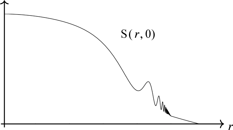

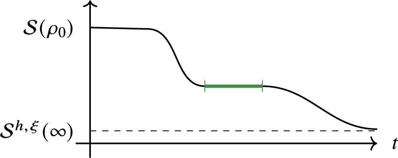

 Open access

