


INTRODUCTION
In the recent years, the growing interest in understanding rapid changes in the cryosphere dynamics has promoted passive seismology as a major tool in the field of glaciology (Podolskiy and Walter, Reference Podolskiy and Walter2016; Aster and Winberry, Reference Aster and Winberry2017). The most common type of observed seismicity is the one generated by ice surface cracking and crevassing, generating the so-called ‘icequake’ signals (Neave and Savage, Reference Neave and Savage1970; Walter and others, Reference Walter2009; Mikesell and others, Reference Mikesell2012; Röösli and others, Reference Röösli2014). In Antarctica, the majority of these surface icequakes involves dynamic processes in extensional regime at the ice-sheet margin such as during ice shelf rifting (Bassis and others, Reference Bassis2007; Heeszel and others, Reference Heeszel, Fricker, Bassis, O'Neel and Walter2014) or tide-induced bending (von der Osten-Woldenburg, Reference von der Osten-Woldenburg1990; Barruol and others, Reference Barruol2013; Lombardi and others, Reference Lombardi2016). Surface cryo-seismicity induced by variations in thermal stress also exists but its investigation remains so far limited to few examples: on ice sheet (Nishio, Reference Nishio1983; Lough and others, Reference Lough, Barcheck, Wiens, Nyblade and Anandakrishnan2015), on sea ice (Crary, Reference Crary1955; Milne, Reference Milne1972; Xie and Farmer, Reference Xie and Farmer1991; Lewis, Reference Lewis1994) and recently on temperate glaciers (Podolskiy and others, Reference Podolskiy, Fujita, Sunako, Tsushima and Kayastha2018) and on ice shelf (MacAyeal and others, Reference MacAyeal2018). Although thermally induced icequakes have small amplitudes and their penetration depths are likely very superficial (few cm to 1 m), and thus do not present a direct threat for ice sheet or ice shelf stability, they may be of large interest for understanding ice and snow mechanics, and also to potentially monitor the thermal state of the ice sheet and its long-term variations. Thermal stress is a natural phenomenon that likely also affects, at longer timescales, the surface of the outer planet icy moons (e.g. Ferrari, Reference Ferrari2018). Detailed investigations of such processes on Earth may, therefore, be of interest in the light of future space science missions that may envision seismic measurements (Panning and others, Reference Panning2018; Vance and others, Reference Vance2018).
To our knowledge, the works of Nishio (Reference Nishio1983) and Lough and others (Reference Lough, Barcheck, Wiens, Nyblade and Anandakrishnan2015) are the only investigations of the thermal stress seismicity of the Antarctic ice sheet. The pioneering work of Nishio (Reference Nishio1983) provided a very comprehensive insight into the occurrence of the so-called ‘snowquakes’ related to thermal stress during an 8-month period near the Mizuho base (70°42′S, 44°20′E, a Japanese base presently abandoned) located on the edge of the Antarctic plateau at 2230 m a.s.l. The author showed that the snowquakes preferentially develop in two situations: during summer at night time when snow temperature decreases when incoming solar radiation is minimum and during winter associated with inland high-pressure atmospheric system. He attributed those events to snow thermal contraction associated with the formation of few-cm-wide thermal cracks penetrating the surface down to ~1 m. More recently, re-analyzing the TAMSEIS and GAMSEIS seismic dataset, Lough and others (Reference Lough, Barcheck, Wiens, Nyblade and Anandakrishnan2015) found ‘firnquakes’ detectable at distances as large as several hundreds of km. They attributed these events to wind-glazed macrocracks formation in the firn layer. Despite the lack of information relative to temperature, the authors interpret these events as resulting from the cooling induced by persistent katabatic winds leading to firn thermal contraction.
The present paper aims at complementing those studies, providing local observations of thermal stress-induced seismicity over a whole year (February 2012 to January 2013) by using data recorded by permanent seismic and weather stations installed near the Princess Elisabeth Antarctica base (71.94°S, 23.34°E, hereafter referred to as ‘PEA’), located ~180 km from the coast and ~1400 m a.s.l. in the escarpment zone of the East Antarctic ice sheet.
SEISMIC OBSERVATIONS
Detection of icequakes
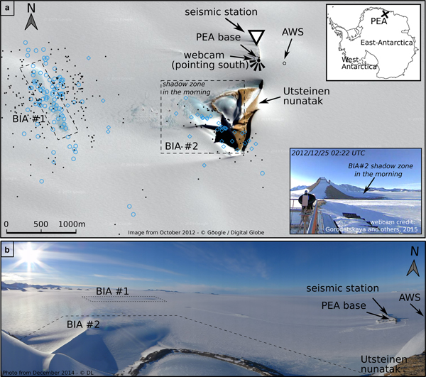
Since 2009, a seismic instrument has been operating near PEA, eastern Dronning Maud Land, East-Antarctica. It sits on a narrow, elongated granitic ridge as an extension of the imposing pyramid-shaped Utsteinen nunatak (Fig. 1) protruding 300 m above the surface of the ice sheet. The instrument is a broadband seismometer with a flat response within the 120 seconds to 100 Hz band, with 24-bit digitizer sampling at 100 Hz. The proximity of PEA (~350 m) provides an easy ground access and reliable power supply to the seismic station.
Location map of the study area (a). The seismic station is marked with a white triangle. The automatic weather station (AWS) is indicated by an open hexagon. The locations of thermal icequakes are marked with open circles for cluster #1 and open diamonds for cluster #2. They are concentrated on the two BIAs marked by two dashed rectangles. The black dots illustrate the location variability using velocity ranges around the mean values (see text). The upper right inset shows the location of PEA base on the Antarctic continent. The lower right inset shows a webcam view from PEA towards the Utsteinen nunatak from 25 December 2012 at 02:22 UTC. In the morning (UTC time), the nunatak, protruding 300 m above the ice surface, creates a prominent shadow zone on its western flank where the BIA #2 is located. The photograph, taken near the summit of the Utsteinen nunatak on 26 December 2014 at ~18:00 UTC and pointing west, shows the location of the two BIAs relative to PEA (b).

We investigated continuous seismic recordings of this permanent seismic station throughout the period February 2012 to January 2013, which is the longest available period of recordings with no data gaps. The data were bandpass filtered between 5 and 20 Hz. Detection of short duration local events was performed using the conventional triggering technique based on the ratio of short-term average over long-term average (STA/LTA, Allen, Reference Allen1978). Durations of 1.5 and 40 seconds were used for STA and LTA windows, respectively. A STA/LTA threshold of 20 and subsequent visual inspection allowed to detect more than 5000 seismic events. Visual inspection revealed a high degree of similarity between most of these events. We, therefore, decided to proceed using cross-correlation-based detection technique selecting, as master events, five waveform patterns with the largest amplitude and initially found via the STA/LTA detection technique. A 2-second long window on the vertical component was first used to detect similar seismic waveforms and subsequent correlation search was performed with the two horizontal components to accept seismic events meeting cross-correlation values higher than 0.50. In total, 4200 events were extracted using this technique. To classify the icequakes and to provide clusters of events, a hierarchical clustering analysis was performed. The waveform cross-correlation value based on a 1 second window encompassing the surface wave arrivals was used to construct a correlation matrix for the entire event dataset. Starting from single-event clusters, the procedure iteratively creates agglomerative clusters of correlated events using the average method to characterize the distance between clusters. This procedure allowed the extraction of five major clusters of events, each gathering at least 100 events, representing a total of 2200 events, i.e. 50% of the original event dataset (Fig. 2). Overall, these events show a weak P-wave arrival followed by larger amplitude surface waves in the 10–20 Hz frequency range and some variable energy above 20 Hz depending on each cluster. No clear S-wave is observed. The signals are characterized by very short duration (<2 seconds) and high-frequency content (up to the Nyquist frequency) suggesting a source located in the vicinity of the station, probably within a few km. Based on the maximum duration of the seismic signal, we evaluated the maximum magnitude Md of this icequake to be ~0.5 (Lee and others, Reference Lee, Bennett and Meagher1972).
Three component stacked traces for the five major clusters of seismic events (a,c,e,g,i). The cluster number and the associated number of events are given. Spectrograms for the vertical component below each cluster traces (b,d,f,h,j) indicate that all clusters present weak first arrivals, strong energy at 10–20 Hz with a dispersive character and signal of variable energy above 20 Hz.

Temporal occurrence of icequakes
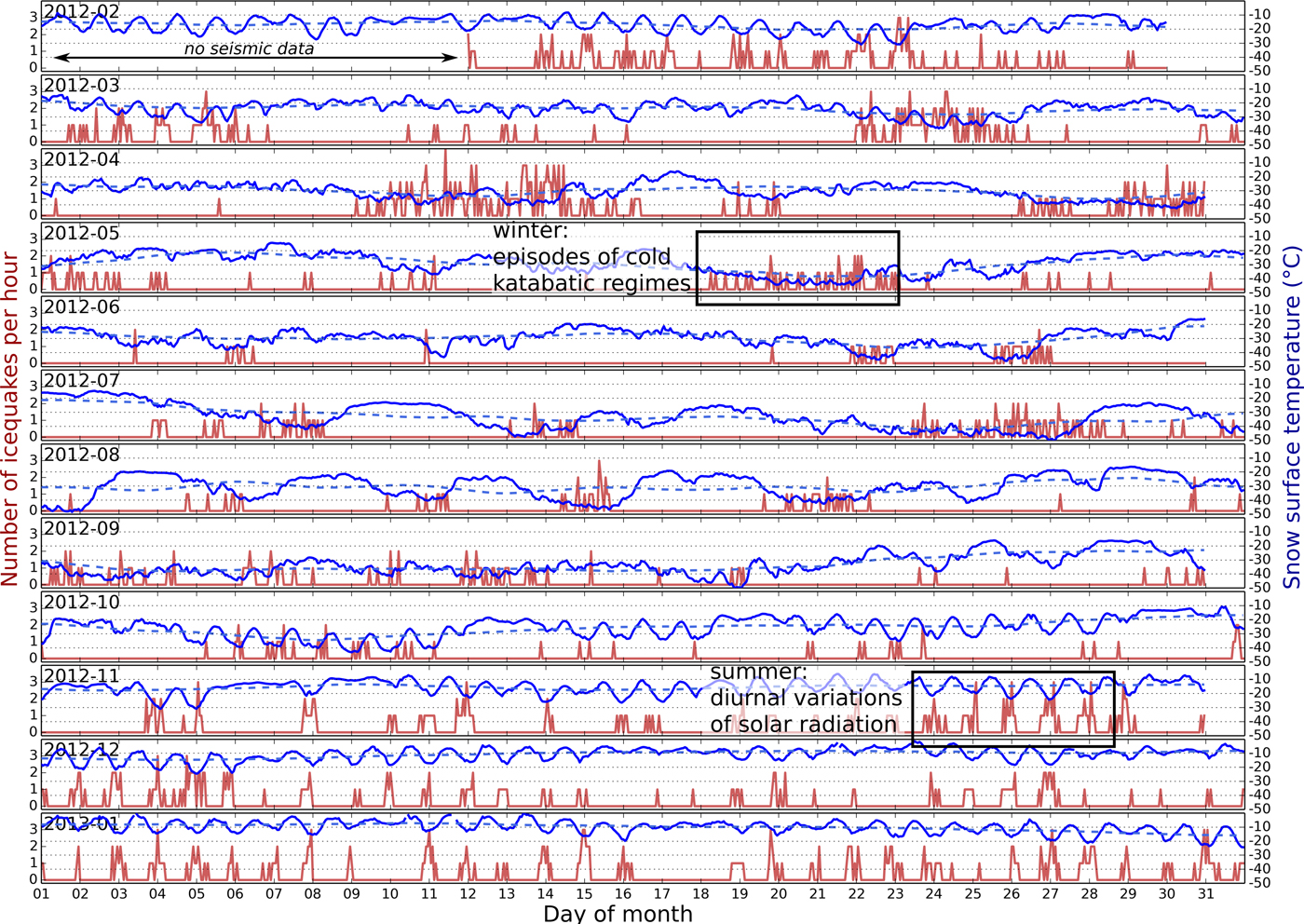
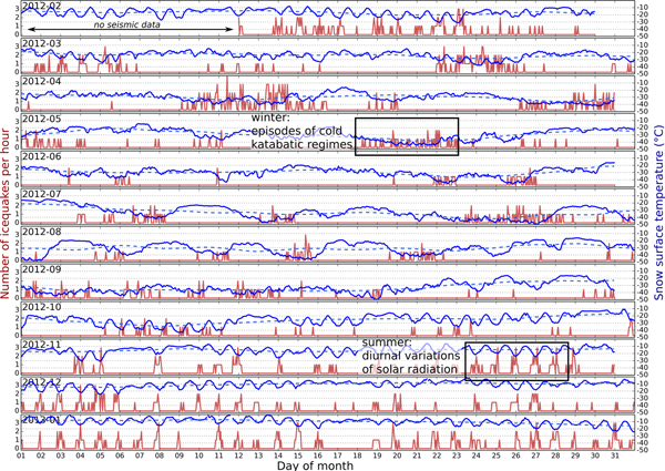
The local ice around PEA is almost motionless, with a maximum ice flow speed <2 m a−1 (Pattyn and others, Reference Pattyn, Matsuoka and Berte2010; Rignot and others, Reference Rignot, Mouginot and Scheuchl2011). This is likely the result of a combined effect of local bedrock topography together with the absence of any outlet glacier or ice stream in the close vicinity. This is confirmed by the absence of macro-scale crevasse fields in the vicinity of PEA (Fig. 1). The observed seismic events are therefore unlikely to be generated by dynamic processes related to ice flow suggesting instead a strong control by environmental factors such as ice/snow surface temperature variations. To test this hypothesis, we first inspected the monthly variations of the occurrence of these events, considering that the surface temperature may vary between summer (October–March, characterized by strong solar radiation) and winter (April–September, characterized by the polar night). For each month, the occurrence of the two major clusters gathering 1500 events, i.e. ¾ of the dataset is merged to consider the dominant source mechanisms. This reveals that the total number of events per hour is two times larger in summer time than in winter time. This first observation leads us to investigate in more detail the monthly and daily variations of these cryoseismic signals through the analysis of hourly mean surface temperature estimated from longwave radiation measurements recorded at an automatic weather station (AWS) located 500 m south-east of the seismic station and installed on a snow surface (Gorodetskaya and others, Reference Gorodetskaya2013, Reference Gorodetskaya2015; Fig. 1a). Figure 3 shows that overall the highest number of events occurs when the snow surface temperature is the lowest. We also observe a clear diurnal modulation of the seismicity related to temperature for the summer months, the maximum amount of icequakes occurring at night. This diurnal modulation ceases in early winter (April–May), as the daily temperatures slowly decrease and the polar night sets in. The seismicity then seems to initiate only at a temperature below −30 °C. The winter period (June–September) is hence characterized by fewer seismic events, mostly clustered during few cold days when snow surface temperature drops below −30 °C. Outside these cold days, seismicity is negligible.
Monthly variations of the number of seismic events per hour gathering the two major event clusters of Figure 2 (red) as a function of hourly mean snow surface temperature (blue, AWS data from Gorodetskaya and others, Reference Gorodetskaya2013). Snow surface temperature is calculated using measurements of outgoing longwave flux (LWout) emitted by the surface and using the relation LWout = ε. σ. (Tsnow_surface)4, where ε is snow emissivity assumed to be equaled to 0.98 (Wiscombe and Warren, Reference Wiscombe and Warren1980) and σ is the Stefan–Boltzmann constant and equals 5.6704 J.s-1.m-2.K-4. The weekly moving average ice surface temperature is shown as dashed blue line.
These observations highlight a temperature dependence of the recorded seismicity. The observed seismic events may, therefore, be attributed to the opening of surface cracks presumably generated by internal snow/firn/ice contraction during surface cooling periods. These particularly cold periods are observed with a daily recurrence in summer due to large diurnal variability in the incoming solar radiation and occasionally in winter characterized by katabatic winds from the Antarctic plateau and clear sky conditions associated with strong surface cooling. This is also illustrated by Figure 4 that displays the number of events for the two main clusters as a function of the time of the day together with the hourly temperature for three periods of the year and the annual mean.
Number of icequakes per hour per month for three periods of the year (summer manned and non-manned months, and winter) and for event cluster #1 (a) and cluster #2 (b). Mean hourly snow surface temperatures corresponding to each of three periods are shown in c (UTC time). The annual mean is also shown for each panel (dashed grey line). The few gaps within the lines indicate that no icequakes were detected at the corresponding time. The approximate start and end time of working hours (for the manned period) are marked by downward arrows (a). The period of extended seismicity for cluster #2 from 02:30 to 04:30 is also indicated (b).
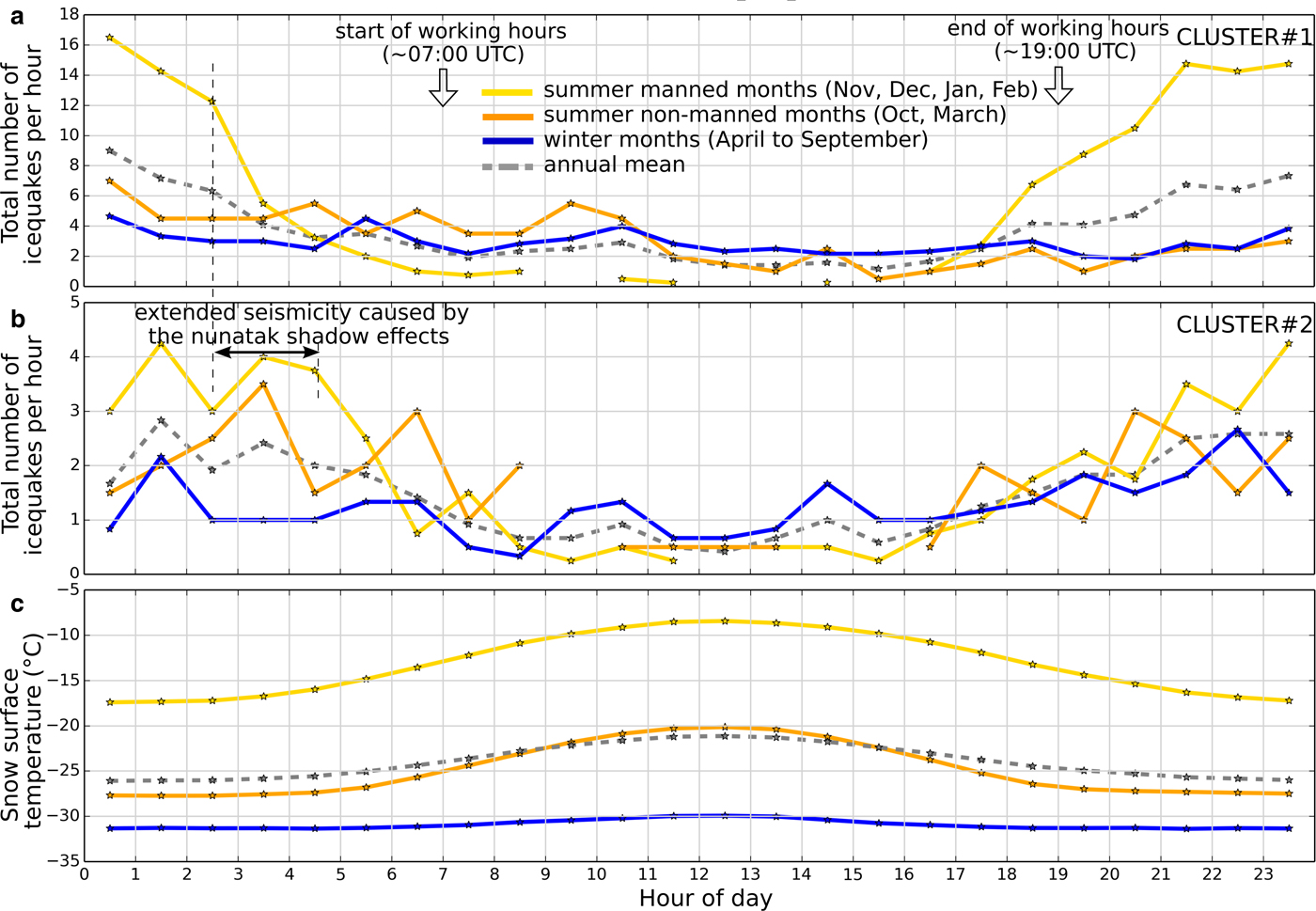
During summer months (November–February, Figs 4a and b, yellow line) we clearly observe higher seismic activity at the beginning and at the end of the day, generally associated with the daily coldest temperature. There is a drastic decrease in seismic activity around midday when the daily temperatures are the warmest. For example, for cluster #1, in summer months, 85% of the events occur in the time interval 18:30–02:30 (Fig. 4a). Interestingly, for cluster #2, to gather 85% of the events the time interval has to be enlarged for 3 hours (i.e., from 18:30 till 05:30, Fig. 4b). This peculiar observation is further addressed in the section Discussion (‘Temporal occurrence’). Note, however, that for this period of the year (November–February), PEA is manned and therefore the number of seismic events recorded during the working hours (approximately from 07:00 till 19:00 UTC) is likely underestimated due to higher noise level present in the seismic data induced by higher anthropogenic activity. However, the drastic decrease of event number in the morning is most likely real as it initiates at 02:30 and 04:30 for cluster #1 and #2, respectively, i.e. well before the beginning of the working hours. If the observed seismic event distribution would be shaped by the lack of detection during daytime, due to anthropogenic noise, one would instead observe a step-like distribution starting ~07:00 rather than the wide and smooth U-shape distribution as it is observed here. For mid-season (October and March, Figs 4a and b, orange line) the decrease in the number of seismic events around midday is also observed but the overall decrease is less pronounced than for the summer months. During the winter period (April–September, Figs 4a and b, blue line) there is no more temperature dependence of seismic events, their number being almost constant over the whole day. The effect of the wind on the initiation of events can be also discarded as it would generate continuous seismic noise rather than individual events as observed here (Withers and others, Reference Withers, Aster, Young and Chael1996). The wind would have an effect on the observations by lowering the signal-to-noise ratio, thus decreasing the total number of detected events. Additionally, at PEA, annual mean wind speed is relatively low compared to most places in Antarctica (Thiery and others, Reference Thiery2012; Gorodetskaya and others, Reference Gorodetskaya2013; Souverijns and others, Reference Souverijns2018). For the time period considered here, the mean wind speed is 4.5 m s−1 with a slight increase to 5.0 m s−1 during the winter period. Indeed, the seismic dataset at PEA does not present any particularly higher noise due to wind perturbations in winter. Therefore, though it may lower the signal-to-noise ratio of the entire dataset, wind perturbations may affect summer and winter observations in a similar manner.
Icequake signal waveforms and locations
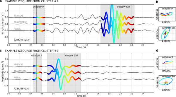
Our procedure of detection leads to two major clusters of icequakes representing ¾ of our initial dataset. The most abundant cluster #1 clearly presents seismic signals of longer duration and lower frequency content than cluster #2, suggesting the former may be generated by a more distant source, yet at few km to PEA. However, both clusters exhibit signals dominated by surface waves suggesting that both originate from sources located at the surface though recorded from different epicentral distances. Icequake signals present a weak emergent P-wave, no S-wave and well-defined surface waves arriving at 1.2–1.3 seconds and 0.2–0.3 seconds after the P-wave onset for cluster #1 and cluster #2, respectively (Fig. 5). Overall, polarization analysis of the three components indicates a near horizontal propagation for the P-wave and back-azimuths pointing to ~255° and ~215° for cluster #1 and cluster #2, respectively (Montalbetti and Kanasewich, Reference Montalbetti and Kanasewich1970; Jurkevics, Reference Jurkevics1988). Surface waves present retrograde elliptical particle motion with varying polarization from elliptical to linear suggesting a propagation in a rather heterogeneous or/and anisotropic medium (Picotti and others, Reference Picotti, Vuan, Carcione, Horgan and Anandakrishnan2015; Diez and others, Reference Diez2016).
Examples of two individual icequake events from cluster #1 (a) and cluster #2 (c). Three component seismograms are rotated into radial and transverse coordinates. Particle motion associated with time windows (shaded in grey in a and c) around the P-wave (‘window P’) and the surface waves (‘window SW’) are shown in (b) and (d). Linear, near horizontal motions characterize the P-waves while retrograde elliptical motions indicate typical surface waves.

Due to the dominance of the surface waves, the events highlighted in our study resemble the ones documented by Lough and others (Reference Lough, Barcheck, Wiens, Nyblade and Anandakrishnan2015). However, though weak, P-wave phases are visible in our dataset. Their absence in the observations of Lough and others (Reference Lough, Barcheck, Wiens, Nyblade and Anandakrishnan2015) was most likely due to attenuation over hundreds of km long epicentral distances. In the study of Nishio (Reference Nishio1983), there is not enough information on the seismic waveform to allow such a comparison. Regarding our observations, the high-frequency content (i.e. 10–15 Hz) of the surface waves indicates they probe the first tens of meters, i.e. uppermost firn layers confirming a shallow source (Picotti and others, Reference Picotti, Vuan, Carcione, Horgan and Anandakrishnan2015). This is also supported by the near-horizontal polarization of the first P-wave as illustrated by Figures 5b and d. In order to quantify the source epicentral distance, we measured time delays between the P-wave and the surface wave arrivals. Such an approach is unfortunately limited to events with a large signal-to-noise ratio with clear P-wave onset, representing here 95 and 38 events for cluster #1 and #2, respectively. The first P-wave can be reasonably assumed to propagate mostly within the uppermost bedrock layers since the station lies on a rock outcrop and the rock basement around the station is shallow (<500 m, Pattyn and others, Reference Pattyn, Matsuoka and Berte2010; Fretwell and others, Reference Fretwell2013). We considered a range of P-wave velocities of 5.3–5.7 km s−1 with the upper limit being the mean value found for upper-crust propagation within the area (Camelbeeck and others, Reference Camelbeeck, Lombardi, Collin, Rapagnani and Martin2019). While the P-wave travels through the uppermost bedrock layers, the surface waves, as pointed out previously, likely probe the firn layers, propagating at velocities in the range 1400–1600 m s−1 when considering 10–15 Hz surface waves (Fig. 9 of Picotti and others, Reference Picotti, Vuan, Carcione, Horgan and Anandakrishnan2015; Diez and others, Reference Diez2016). Combining these velocities, the time delays between the P-wave and the surface wave arrivals, together with the azimuthal information from polarization analysis (Fig. 5) provide a reasonable estimate of possible icequake locations with uncertainties in the order of ±0.5 and ±0.25 km for cluster #1 and cluster #2, respectively. The event locations focus univocally towards a rectangle shaped blue ice area (BIA) and towards the Utsteinen nunatak and its surrounding wind-carved BIAs located 4 km south-west and 1 km south-south-west of the station for cluster #1 and cluster #2, respectively (Fig. 1). Interestingly, while located about three times closer to PEA, cluster #2 exhibits about two times fewer icequakes than cluster #1. This may be due to a complex subsurface propagation caused by the presence of a three-dimensional bedrock structure, reflected at the surface by the pyramid-shaped Utsteinen nunatak. This complex propagation may result in varying seismic waveforms and fewer detections for cluster #1. With their location on the leeward side of the nunatak, these two BIAs likely result from wind scouring effects on the surface, removing readily any deposited snow (BIA of type I in Bintanja, Reference Bintanja1999). We attribute the observed seismicity to be generated by these BIAs responding to thermal cooling of the surface. This does not imply there are no thermal icequakes within the snow/firn covered areas surrounding the seismic station. If any, they may not be located in confined areas but may rather be spread all around the station, generating varying waveforms and thus may not be detected via our waveform pattern recognition procedure.
DISCUSSION
Temporal occurrence
Over the year-long dataset, 1500 seismic events were detected and categorized into two clusters based on their seismic waveforms and durations. Their source location on two BIAs and their dependence on large diurnal temperature variability mainly due to daily solar radiation in summer or cold katabatic regime in winter suggest they are associated with thermal contraction of blue ice. Our dataset shows a clear temporal pattern of icequake occurrence that deserves to be discussed in the light of the few previous analyses of similar events. In the study of Lough and others (Reference Lough, Barcheck, Wiens, Nyblade and Anandakrishnan2015) no systematic and long-term temporal analysis was unfortunately provided as the dataset originated from short-term experiments. However, a high rate of ‘firnquake’ activity was observed during the onset of the Antarctic winter consistent with thermal contraction. Regarding the study at the inland Mizuho base by Nishio (Reference Nishio1983), a detailed analysis of the temporal occurrence of the so-called ‘snowquakes’ was provided and appears similar to ours. The author showed that the ‘snowquakes’ activity suddenly occur when temperature starts to decrease in the early afternoon, reaches a peak at night and progressively ceases in the morning. The ‘snowquake’ activity is described as irregular during winter, modulated by the inland high atmospheric pressure system. It presents, however, a diurnal modulation in early summer (mid-September to the end of November), due to variation in daily solar radiation. Surprisingly, the author observes that the activity ceases in summer (end of November to early January) where one would expect abundant seismicity due to large temperature fluctuations as in our study. Nishio explains this observation by the dominant ductile deformation of snow for temperature above −20 °C, a phenomenon not seen for instance in the most recent studies by Podolskiy and others (Reference Podolskiy, Fujita, Sunako, Tsushima and Kayastha2018) and MacAyeal and others (Reference MacAyeal2018). However, at Mizuho base, the surface conditions and mean air and surface temperatures differ significantly from these two studies. Our observations, which also do not present such a lack of seismicity at these warm temperatures, may indicate that icequake sources are likely located in a medium different from the snow, i.e. ice.
Interestingly, a closer look at the daily occurrence of our two clusters reveals that the seismicity rate decrease we observe in the morning does not occur at the same time as one would expect for two close-by ice surfaces with similar rheological properties (Fig. 4). Indeed, considering the summer period, while the number of events from cluster #1 drops at 02:30 AM, cluster #2 starts decreasing 2 hours later. Images from a webcam pointing towards the Utsteinen nunatak confirms that, during summertime in early morning, the BIAs of cluster #2 is shadowed by the 300 m high (above ice surface) nunatak for 2 hours after sunrise (Fig. 1 bottom right inset, Gorodetskaya and others, Reference Gorodetskaya2015), leading to cold temperature persistent for two additional hours on BIA #2 while BIA #1 is already receiving solar radiation. This delay is not observed in the late afternoon when the seismicity initiates simultaneously for both clusters. Indeed, in the late afternoon, both BIAs, located on the western side of the nunatak, undergo the same solar radiation decrease with no obstacle creating any shadow effect (Fig. 1b). This observation of a 2 hour delay in the decrease of seismicity further supports the location of cluster #2 on the western flank of the nunatak. It, therefore, favors the interpretation of icequake induced by thermal stress variations, controlled in summer by the solar radiation over the blue ice.
Dependence on absolute temperature and on its temporal change
Our year-long analysis of icequakes shows that most of our events occur during summer time when the daily mean temperature variability is significant, i.e. >10 °C, due to significant incoming solar radiation variations (Fig. 4, yellow curve). Yet, our detection shows that about one-third of our events occur in the winter period when daily temperature fluctuations are rather small (Fig. 4, blue curve). These observations lead us to address the question of the absolute temperature dependence of those icequakes by analyzing their number and amplitude for daily mean surface temperature T mean and mean temperature change ∂T/∂t (Fig. 6). Having determined that the observed icequakes are originating from two BIAs and lacking meteorological measurements directly at the BIAs, we use the measured snow surface temperature in the AWS site located 1 km from the nearest BIA to infer temperature variability. In order to relate to the BIAs temperature, we use measurements on the BIA and on the snow surface in a similar environment at Svea station (see Appendix A, Figs 8 and 9). In summer, BIA surface temperature may be several degrees warmer than snow (Takahashi and others, Reference Takahashi, Endoh, Azuma and Meshida1992; Bintanja and van den Broeke, Reference Bintanja and van den Broeke1995; Bintanja, Reference Bintanja2000), owing to its lower albedo value (i.e. ~0.6 compared to >0.78 for fresh snow, e.g. Winther and others, Reference Winther, Elvehøy, Bøggild, Sand and Liston1996; Reijmer and others, Reference Reijmer, Bintanja and Greuell2001). This is demonstrated by Figure 9a for Svea site. Stronger surface radiative heating, together with higher thermal conductivity and lower extinction coefficient of blue ice compared to snow (Yen, Reference Yen1981; Fukusako, Reference Fukusako1990) result in warmer ice subsurface layers (<1 m depth) that undergo higher temperature change at least in summer time when solar radiation is maximum (Bøggild and others, Reference Bøggild, Winther, Sand and Elvehøy1995; Bintanja, Reference Bintanja2000). Indeed, reported observations indicate that the daily temperature fluctuations induced by solar radiation penetrates the ice down to 80 cm depth while this penetration depth is about twice shallower for snow layers (Nishio, Reference Nishio1983; Bintanja, Reference Bintanja2000). On the other hand, in winter, the snow surface temperature is primarily controlled by longwave radiation and turbulent fluxes which do not depend on the ground albedo. However, both longwave radiative and turbulent fluxes vary strongly with the alternation of cold katabatic and warm synoptic regimes affecting both the snow and BIAs (Thiery and others, Reference Thiery2012; Gorodetskaya and others, Reference Gorodetskaya2013; Souverijns and others, Reference Souverijns2018). Our analysis at Svea (Fig. 9) showed that for winter periods, snow and ice surface temperature show similar absolute values and synoptic-scale variability, while subsurface temperatures (initially installed at 10 cm depth) at BIA show colder minimum temperatures and warmer maximum temperatures compared to the snow site (this can be caused also by increase in the depth at the snow site due to snow accumulation subduing the subsurface temperature variability).
Distribution of number (a) and normalized RMS amplitude (b) of cluster#1 icequakes for mean surface temperature Tmean (vertical axis) and hourly temperature change ∂T/∂t (horizontal axis). Values are given by the top color bars. The number (n days) within each box indicates the numbers of days where icequakes were detected. Label ‘0 days’ means that the year 2012 did not contain such a pair of Tmean and ∂T/∂t. The side panels represent the mean value for each Tmean (left vertical panel) and for each ∂T/∂t (bottom horizontal panel). The rate of temperature change is defined as the mean temperature decrease per hour per day.

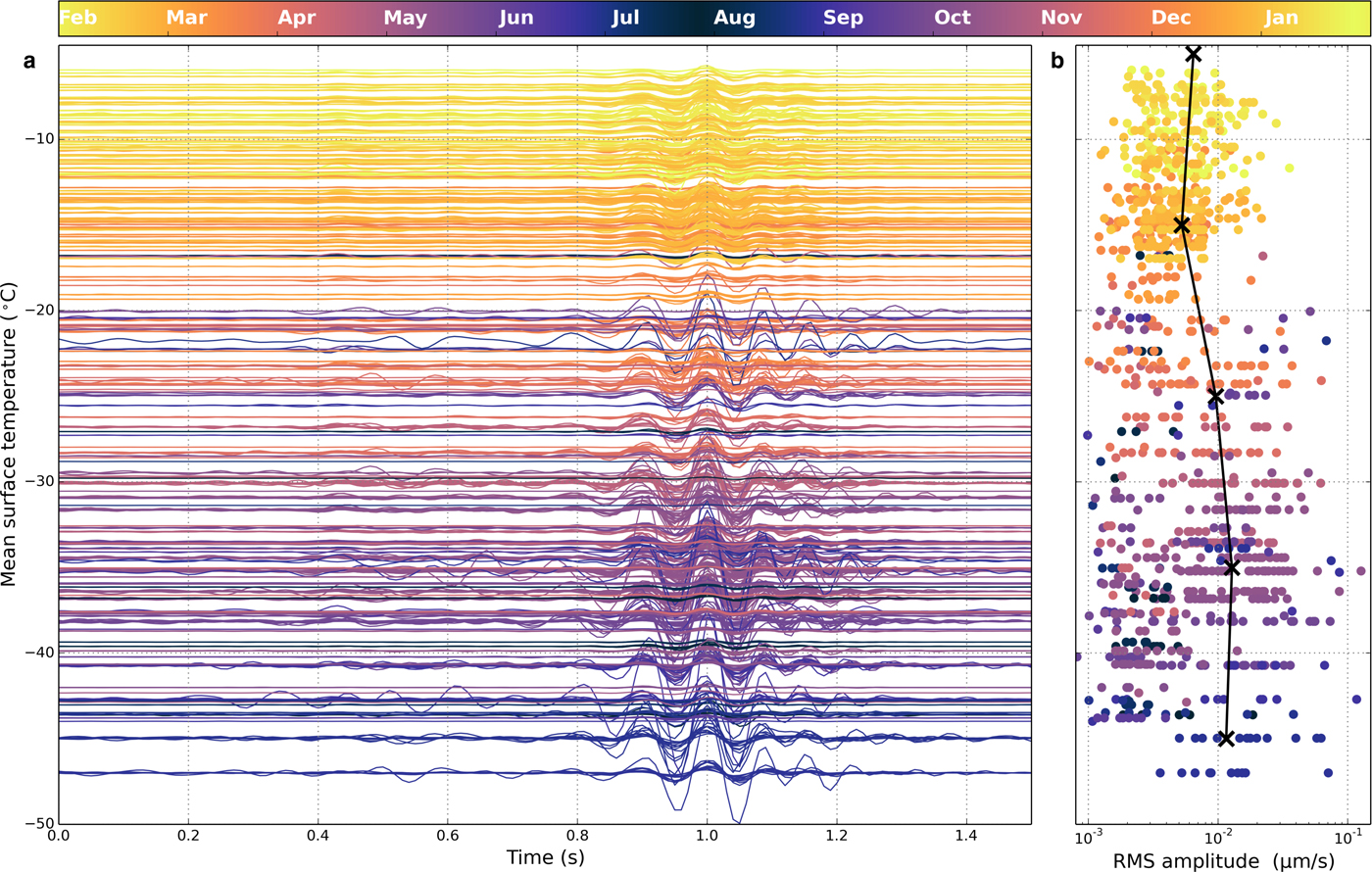
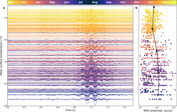
Bearing these considerations in mind, we present in Figure 6 the variations of icequake number and amplitude for the most abundant cluster #1 as a function of surface temperature and its time derivative, as estimated on the snow surface at the AWS site, 500 m south-east of PEA. These summarizing heatmap representations show that for the increasing rate of temperature change, we observe increasing icequake numbers (Fig. 6a, bottom horizontal panel). This is observed for all temperature ranges except for extremely cold temperature, i.e. < −30 °C, corresponding to the end of summer. There, the initiation of seismicity is more rapid (Fig. 6a, left vertical panel) i.e. the icequake number is significant even for small rate of change, for example, there are four icequakes per day for 0.4–0.6 °C h−1 at T mean = −30° to −40 °C while there are only 0.5 icequakes per day for the same rate at T mean = −20° to −30 °C. Regarding the distribution of icequake amplitude, no particular correlation with the temperature change is observed (Fig 6b, bottom horizontal panel). However, seismic amplitudes appear to be anticorrelated with temperature (Fig. 6b, left vertical panel). This observation is well illustrated in Figure 7 that presents the vertical component of seismic traces for cluster #1 as a function of the daily mean temperature. For ‘warm’ temperature, i.e. Tmean > −20 °C, icequakes are characterized by low amplitudes and small variability (Fig 7). In contrast, when the temperature drops below ~−20 °C, the icequake amplitude increases, so as its variability among various events. Considering that all detected icequakes shown in Figure 7 originate from the same source location (Fig. 1, BIA #1), and therefore that the amplitude variations are not caused by varying epicentral distances, this indicates a clear link between the seismic energy released by thermal icequakes and the surface temperature.
Vertical component of seismic traces (a) and associated RMS amplitude (b) of cluster #1 icequakes sorted as a function of daily mean temperature. The connected crosses in (b) indicate the mean RMS amplitude for each temperature bin as defined in Figure 6. Color represents the time of the year as indicated in the top color bar.
Ice rheology proscribes thermally induced strain rate initiation of new fractures to explain the origin of icequakes. Indeed, the thermal strain rate (defined as $\dot{\varepsilon} = \alpha \;. \; \; \partial T/\partial t\; \;$ with α ≈ 5.10−5 °C−1 being the coefficient of thermal expansion of ice (Butkovich, Reference Butkovich1959)) is of the order of 10−8 s−1, i.e. at least one order of magnitude below the ductile – brittle transition of ice (Schulson and others, Reference Schulson, Lim and Lee1984; Lee and Schulson, Reference Lee and Schulson1988). Therefore, BIAs likely accommodate the induced thermal stress mostly via elastic or creep deformation (Sanderson, Reference Sanderson1978) and, as described hereafter, via reactivation of pre-existing fractures. Indeed, to explain our detected seismicity, considering the previous observations (Figs 6 and 7), we propose the following processes. The relatively sudden increase of icequake number for temperatures < −30 °C, contrasting with a slow increase towards higher rate of temperature change for warmer temperatures (Fig. 6a), may indicate a change in the mechanism at the origin of the icequakes rather than a change in the ice properties that would not be so abrupt. Considering that thermal icequakes are likely due to cyclic opening/closing of existing superficial cracks (Nishio, Reference Nishio1983), we surmise here that, at the end of summer (end of March), when solar radiation ceases and temperatures remain below −30 °C for longer time periods (from several days to more than a week), opened cracks prevail. We postulate that the underlying mechanism in triggering the icequakes is the propagation of fractures at the tips of the opened cracks where stress concentrates. This differs substantially from the nocturnal re-opening of pre-existing cracks, prevalent during summer. Furthermore, at a constant fabric and grain size, the temperature is a major controlling factor of the ice rheology. As the temperature decreases, the effective viscosity of ice increases significantly, for example, by a factor of 5 for a temperature drop from −10 to −25°C (Cuffey and Paterson, Reference Cuffey and Paterson2010). The ice becomes stiffer and may support higher stress before failure. The stress relaxation may occur through large amplitude icequakes, which may explain the progressive increase in amplitude of icequakes with decreasing temperature (Fig 6b, vertical left panel).
In the absence of more quantitative information on the blue ice temperature and on direct thermal crack observations nearby PEA, these interpretations remain open to discussion. Indeed, as discussed already (see the Appendix for details), the warm temperatures presented in Figure 6 most likely underestimate the actual blue ice temperatures, and may occasionally approach the ice melting point (see also the Appendix Fig. 8 comparing blue ice and snow temperatures at Svea station). Localized surface ice melting and refreezing may occur and participate in crack healing (Colbeck, Reference Colbeck1986). As an opposite mechanism, thermal fatigue may play an important role in creating flaws and microcracks, lowering the ice tensile strength, thus weakening the ice surface, in a way similar to rock weathering (Hall, Reference Hall1999; Lamp and others, Reference Lamp, Marchant, Mackay and Head2017). To obtain more complete insights on the thermal icequakes and on blue ice rheology, a more relevant and dedicated experiment conducted over such BIAs using a multidisciplinary approach should be conducted, including detailed vertical temperature logging in the blue ice.
CONCLUSIONS
By analyzing 1 year of continuous seismic data recorded at the Princess Elisabeth base in East-Antarctica, we detected thousands of icequakes most likely related to thermal stress and affecting two narrow areas in the vicinity of the base, each characterized by outcropping blue ice. Our measurements showed that summer daily solar radiation variations inducing large surface temperature variability and winter surface cooling during the cold katabatic regime, are the main environmental mechanisms triggering this temperature-related icequake seismicity. Investigations on the occurrence of these icequakes indicate that their properties are dependent on both the absolute surface temperature and its time derivative. In this regard, they can be viewed as an opportunity to monitor the thermal state of ablation zones. We surmise that thermal icequakes are abundant in cryo-seismic datasets but are often regarded as noise perturbations and rejected from further investigation. To obtain more complete insights into thermal icequakes and underlying ice fracture mechanics, and to assess the potential of passive seismology to monitor the surface thermal state, we encourage dedicated and integrated studies on both BIAs and snow/firn cover.
ACKNOWLEDGEMENTS
We acknowledge the support of the Belgian Antarctic program lead by the Belgian Federal Science Policy (BELSPO) allowing the installation and maintenance of the seismic station (project GIANT-LISSA, grants EA/33/2A and EA/33/2B). We are thankful to the BELSPO project HYDRANT (grants EA/01/04A and EA/01/04B, PI Nicole van Lipzig) that supported installation and maintenance of the automatic weather station at PEA together with technical support by the Institute for Marine and Atmospheric Research (IMAU), Utrecht University. We thank Carleen Reijmer (IMAU) for providing AWS6 and AWS7 data at Svea base. Niels Souverijns is acknowledged for providing access to the webcam data now supported under BELSPO project AEROCLOUD. We are grateful to the International Polar Foundation for the logistic and field support in such a difficult environment. We are also grateful for constant development of the following open-source software packages used in this study: Python (python.org), Matplotlib (Hunter, Reference Hunter2007), Obspy (Beyreuther and others, Reference Beyreuther2010) and QGIS (qgis.org). We also benefited from the Quantarctica database distributed by the Norwegian Polar Institute (quantarctica.org). IG thanks FCT/MCTES for the financial support to CESAM (UID/AMB/50017/2019), through national funds. We thank Trevor Williams for proofreading the manuscript while at sea. The manuscript profited from constructive reviews from Evgeny Podolskiy and an anonymous reviewer. This is IPGP contribution 4044.
APPENDIX A
SNOW AND BLUE ICE TEMPERATURES AT SVEA STATION
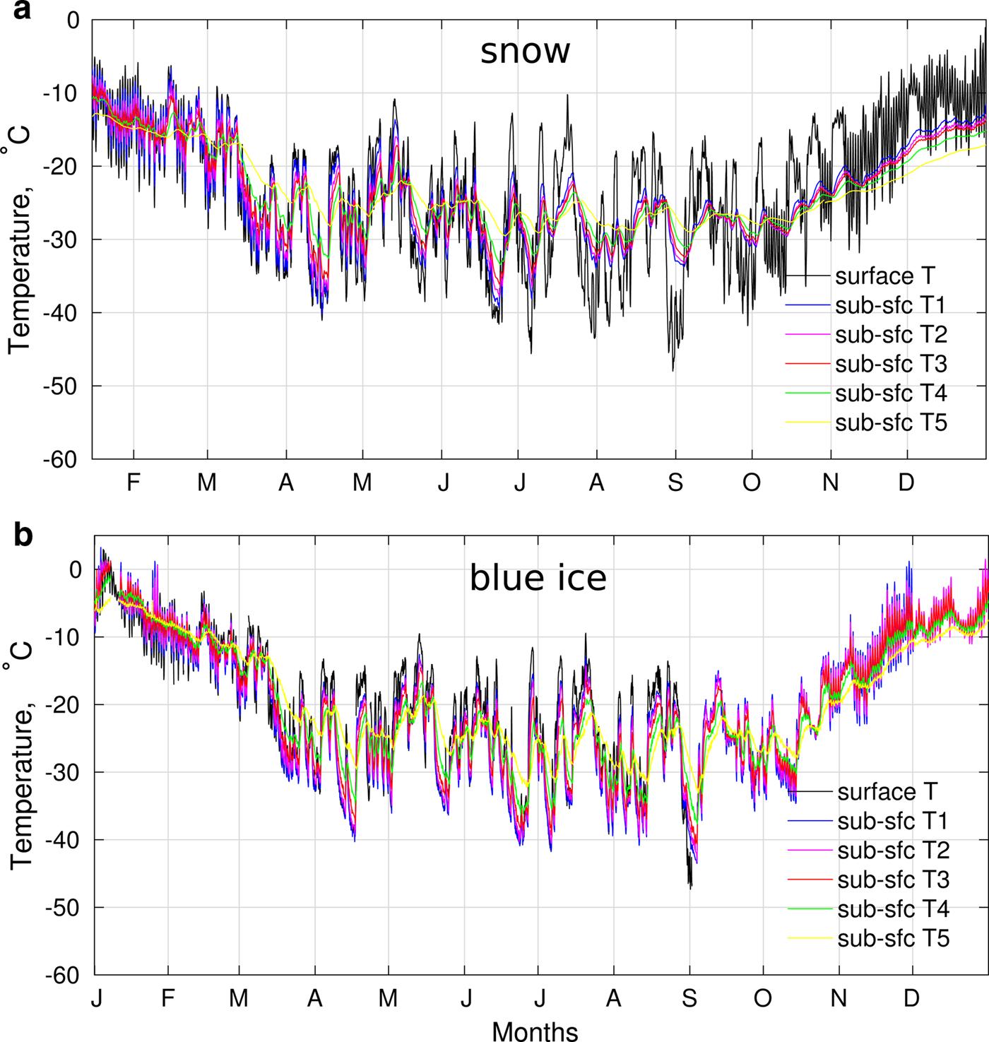
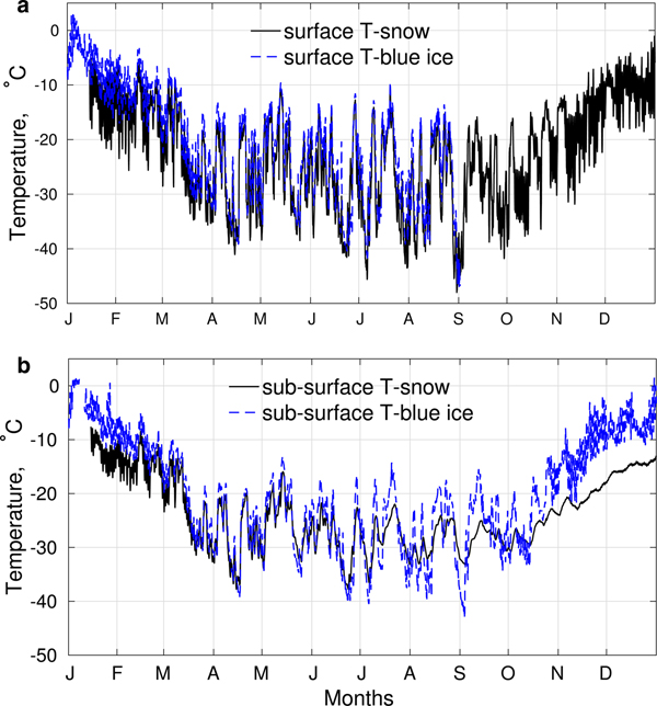
In the absence of temperature measurements at BIAs, our study uses the dataset from the AWS16 located on a snow surface nearby PEA. In order to compare snow and blue ice surface temperature behavior, we used data from AWS (developed by the Institute for Marine and Atmospheric Research – IMAU) nearby Svea station (74°35′S, 11°13′W) located in the escarpment zone of the East Antarctic ice sheet, 350 km from the coast at elevation 1261 m a.s.l. with mountains nearby (Bintanja, Reference Bintanja2000), which is a similar environment to PEA. We compared surface and subsurface temperatures derived from an AWS located on the snow surface and from an AWS located in the BIA (IMAU AWS6 and AWS7 installed at sites 3 and 1, respectively, as described by Bintanja, Reference Bintanja2000) (Figs 8 and 9). Snow and blue ice surface temperatures were calculated using 2-hourly mean measurements of broadband longwave radiative fluxes by pyrradiometers (for sensor description, see van den Broeke and others, Reference van den Broeke, Reijmer, Van As, Van de Wal and Oerlemans2005). Subsurface temperatures were measured using thermocouples initially installed at the depths of 5, 10, 20, 40 and 80 cm on 14 January 1998 at AWS6 and on 07 January 1998 at AWS7. Figure 8 shows surface temperature and subsurface temperatures down to 80 cm (initial installation depth) as measured at the snow and blue ice sites. Figure 9 compares surface and subsurface temperatures at the initial depth of 10 cm at the snow and blue ice sites. Pearson correlation coefficient between the surface temperatures at two sites is 0.95 (significant at 99% confidence interval).
Two hourly mean temperatures for two sites during 1998: AWS6 located on a snow surface (a) and AWS7 located on a blue ice surface (b). Surface temperature is calculated using outgoing and incoming longwave radiation fluxes. Temperatures are measured initially at depths 5 cm (T1), 10 cm (T2), 20 cm (T3), 40 cm (T4) and 80 cm (T5). The actual depth varies depending on accumulation/ablation on snow/ice surface.
Two hourly mean temperatures comparison at two sites for surface temperatures (a) and subsurface temperatures initially at 10 cm (T2) below the snow/ice surface (b). Black solid line is for snow site and blue dashed line is for blue ice site. The actual depth varies depending on accumulation/ablation on snow/ice surface. The dataset of the surface ice blue temperatures (blue dashed line in (a)) stopped on 02 September 1998.

During summer months (here January–February when measurements at both sites are available), blue ice surface temperature is much warmer both during its diurnal maximum and minimum (on average by 5.6 and 4.6 °C for daily maximum and minimum temperatures, accordingly) leading to an average daily amplitude of surface temperatures over blue ice 1 °C larger compared to snow surface. In winter, icequakes are not associated with diurnal temperature variability but rather with long periods of surface cooling with temperature below −30 °C. The analysis of Svea measurements shows that both blue ice and snow surface temperatures are comparable and for temperatures below −30 °C BIAs are on average warmer only by 1.05 °C.
Large daily variability in summer and strong cooling during the winter of subsurface temperatures are important for the thermal stress causing icequakes. The daily variability in subsurface temperatures reduces with depth compared to the surface temperatures (Fig. 8). Snow site experiences snow accumulation during the year, while ablation dominates the blue ice site. Thus, the subsurface temperatures installed at the same initial depth at the snow site show smaller daily variability later during the year compared to the blue ice site. Figure 9 shows a comparison between surface temperatures and subsurface temperature initially at 10 cm depth at the two sites. The subsurface temperature at the blue ice site is warmer compared to the snow site with the daily amplitude 2 °C larger compared to the subsurface temperature at the snow site (mean diurnal variability during summer months is on average 4 °C at the snow site and 6 °C at the blue ice site). During winter the minimum subsurface temperatures at the blue ice site are somewhat colder (on average by 2 °C). As the blue ice site is dominated by ablation, this explains stronger cooling of subsurface temperatures in winter compared to the snow site characterized by accumulation. This comparison of the surface and subsurface temperature behavior at the snow and blue ice sites supports the conclusions of the paper based on the AWS at the snow site.


 Open access