Array figures of merit

In order to reduce the number of measurements used for characterization, we evaluate the performance of the array using three criteria: the power radiated in the main beam direction (MBP), the side lobe level (SLL), and the field of view (FoV) in the E- and H-plane cuts. SLL is here defined as the relative strength of the peak side lobeFootnote ¹ with respect to the MBP and FoV is defined as the range over which the SLL is negative. These measures provide insight into the array’s maximum effective isotropic radiated power (EIRP), 3-dB steering range, and gain, without requiring a full 3D scan.

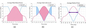
In order to characterize the performance of the array with a single number for optimization purposes, the average MBP and SLL over the FoV, and the average FoV over the different ϕ cuts, are used as the optimization criteria as shown in Figure 2. Using an average ensures that the array performance is over its entire steering range and not just in one direction.

Figure 2.

Visualization of optimization criteria. (a) The main beam power is integrated within the theoretical field of view, e.g. $\pm$$60^{\circ}$. (b) The difference between the main beam power and peak side lobe power, the side lobe level, is integrated within the theoretical field of view. (c) The field of view optimization maximizes the angular difference between the first crossings of the main beam power and the peak side lobe power.

Beams are only steered within the FoV when characterizing the MBP and SLL because, due to spatial aliasing, the phase settings required to steer a beam outside of the FoV are the same as those that steer a beam at a different angle inside of the FoV. Since the beam strength is higher within the FoV, the beam on the outside is not truly the main beam, but a grating lobe of the beam on the inside. The FoV of an ideal λ-spaced array is $\pm 30^{\circ}$, greatly reducing the number of measurements.

Array characterization time

An efficient measurement approach is necessary to perform in-situ optimization. In a radiation pattern measurement, the average time to move the antenna under test between measurement points, T_move, is on the order of seconds, while the measurement time, T_meas, can theoretically be less than a microsecond. Assuming $T_{meas} \ll T_{move}$, the time to characterize a phased array is:

(1)\begin{equation} \begin{split} T_{char} \approx N_{b} (N_{m}+1) T_{move}, \end{split} \end{equation}

where N_m is the number of measurement points per beam and N_b is the number of beams used to characterize the array.

Equation 1 is the fixed time required to move between all the measurement points. If T_move is one second, then it takes 90 minutes to characterize a single meta-gap configuration along two cuts with 5^∘ precision. If M states are measured sequentially than the total measurement time is $M T_{char}$.

Instead, multiple configurations can be measured in parallel by iterating through them at each measurement point. Thus a large number of configurations can be characterized while only moving through measurement points once. In this case, the time to characterize a batch of M configurations is:

(2)\begin{align} T_{batch}& \approx (N_{b} + N_{m})T_{move}\nonumber \\ & \quad + M N_{b}[ N_{m} + (N_{tiles}-1)D] T_{meas}, \end{align}

where N_tiles is the number of tiles and D is the number of measurements required to optimize the beam phase settings.Footnote ²

For a sufficiently large batch size the total characterization time is decreased by orders of magnitude. However, results are not available until the entire batch is processed. Thus algorithms must operate on batches of measurements, as no decision can be made until the completion of each batch. The measurement time of this method of sequential batches is simply Equation 2 times the number of batches.

Characterizing the meta-gap optimization problem

Meta-gaps present a high-dimensional configuration space with a far smaller subspace of useful solutions; a meta-gap structure with k switches has 2^k possible states. Finding an optimal state for this kind of switching network has been proven to be NP-Hard in general and there is no known convex heuristic that consistently identifies solutions close to the optimal one [Reference Lavaei, Babakhani, Hajimiri and Doyle4].

Thus, non-convex heuristic algorithms must be employed in order to identify preferred, if not optimal configurations. While problem-specific heuristics will outperform abstract metaheuristic algorithms [Reference Wolpert and Macready36], it is not obvious how a given set of switches will alter the array behavior due to the strongly nonlinear behavior of switched networks and the complex interactions of parasitic elements in response to different electromagnetic excitations for different steering angles.

Four different metaheuristic algorithms and a simple random search are employed to both explore meta-gap performance and to provide insight into the general structure of the optimization problem and its solutions. The selected algorithms—Genetic Optimization (GEN) [Reference Bremermann37], variable neighborhood search (VNS) [Reference Mladenović and Hansen38], Particle Swarm (PS) [Reference Kennedy and Eberhart39], and Simulated Annealing (SA) [Reference Kirkpatrick, Gelatt and Vecchi40]—ake advantage of different properties of the optimization problem [Reference Sörensen41]. Genetic optimization excels at problems that contain underlying “features” that can be exploited. VNS takes a local to global approach, performing well on problems with clustered optima. SA has the opposite approach, performing a wide area search before settling into a local optima. Like SA, PS takes a global to local approach but incorporates several agents that investigate local optima. Finally, the random search serves as a baseline comparison. Thus, properties of the problem structure can be identified by comparing the relative performance of these methods.

Optimization framework

The same optimization framework is used in both the simulated statistical experiments discussed in Section “Simulated Statistical Analysis” and the in-situ optimization experiments discussed in “In-Situ Optimization Experiments” section. The metaheuristic algorithm selects switch states to be measured, the measurement range (either real or simulated) measures the desired array characteristic for the selected states, and the results are provided back to the algorithm to select the next states to be measured. After a predefined number of iterations, the algorithm is terminated.

As discussed in “Demonstration Array” section, the demonstration array has 2⁹⁶⁰ different possible meta-gap states. In the simulated experiment and the initial in-situ experiment, each meta-gap sheet is constrained to have the same switch settings. The rational for this relatively arbitrary restriction is twofold, first, it restricts the total search space to 2²⁴ possible switch settings and, second, the difference in field perturbations between neighboring states is larger and thus easier to measure. These restrictions are relaxed in the later in-situ experiments.

Due to the complexity of phased array characterization, states are measured in batches in order to reduce the total measurement time. The algorithms operate in batches of 24 states so that search based approaches, like VNS and SA, can evaluate every neighboring state in a single batch during the identical sheet experiments. The algorithms are iterated for 30 batches, thus exploring a total of 720 states.

To ensure consistency, the same tuning parameters, run lengths, and batch sizes are used in the different experiments. This consistency allows direct comparison of the relative performance of the different algorithms both in different experiments and when optimizing different criteria.

Simulation setup

Figure 3 shows the simulation model used for statistical analysis. It is a five element λ-spaced linear array of patch antennas separated by four meta-gap sheets. Both the meta-gap sheets and patch antennas have the same metal patterns and dimensions as their physical equivalent. The meta-gap sheets also model the 30 nH choke inductors in parallel with switches. Figure 3(e) shows the array and the 37 short dipole sensor antennas located in the far-field every 5^∘ in the steering-plane. This model contains 138 ports—5 excitation ports, 37 sensor ports, and 96 control ports—that are represented by teal rectangles. The total simulation volume including the array and sensor ports is $605\pi \lambda^3$.

Figure 3.

Finite element simulation model. (a) The five element λ-spaced array with embedded meta-gaps. (b) Closeup of antenna model with excitation port. (c) Closeup of meta-gap model with control ports. (d) Closeup of dipole sense antenna. (e) Simulation volume with array and sense antennas in the far-field.

The array was simulated using HFSS’s finite element solver over 15 h using 23 cores and 218 GB of RAM. The 138 port s-parameter model derived from the FEM simulation enables the behavior of different meta-gap settings to be quickly calculated. This calculation method is encapsulated into a “simulated range” enabling the same optimization algorithms to be used for both simulated and measured optimization experiments.

It is important to note that the simulated problem is only a one dimensional array instead of the full two dimensional demonstration array used for the in-situ experiments. A simulation of the full 2D array was not possible due to the significantly larger simulation volume required (closer to $7100\pi \lambda^3$) and the larger number of ports (1058).

Algorithmic performance

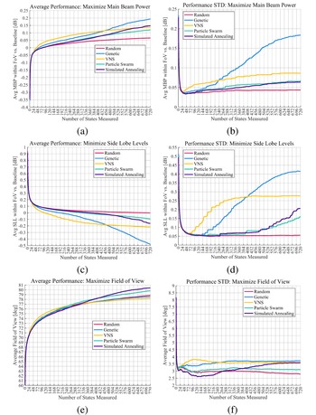
The variable performance of the stochastic algorithms between runs is best described by a probability distribution. Figure 4 compares the average and standard deviations of the algorithms’ performance over time for all three optimization criteria. A general summary of the simulated algorithm performance is shown in Table 1.

Figure 4.

Comparison of the statistical performance of different algorithms over 1000 trials when (a)–(b) maximizing main beam power, (c)–(d) minimizing side lobe level, and (e)–(f) maximizing the field of view. (a), (c), and (e) show the average performance of the best identified state over time. (b), (d), and (f) show the standard deviation of performance of the best identified state over time.

Table 1.

Summary of algorithm performance in simulated experiments.

As can be seen, the algorithms’ behavior when maximizing the MBP are similar to their behavior when minimizing the SLL. For both criteria, genetic optimization performs the best on average, but also has the largest standard deviation for performance between runs. VNS converges rapidly on a local optima, but the standard deviation of the performance of that optima is high. The performance of PS and SA is very similar as they both broadly explore the space before converging on a local optima.

The statistical behavior of the algorithms when optimizing the FoV is quite different. For these criteria, PS and SA both perform the best. The most striking result is that both VNS and genetic optimization perform worse than the random search. However, the difference between the average performances is less than 0.5^∘ and so it is possible that the statistical power of the experiment is not large enough for the difference to be statistically significant. Finally, the algorithms have similar standard deviations in performance when optimizing the FoV.

Distribution of states

Because they are randomly selected, the states measured by the random search algorithm provide a statistical sample of the underlying distribution of states. For each of the optimization criteria, the random algorithm explored approximately 705,000 unique states out of 16.8 million over the 1000 runs.

Figure 5 contains histograms of state performance for the different optimization criteria and thus illuminates the underlying distribution of states. The distributions for MBP and SLL are closely related, with a long tail of states that perform worse than baseline and a sharp drop-off in states that perform better. For MBP optimization, the sample mean and standard deviation are −0.35 and 0.23 dB, respectively, while they are 0.92 and 0.50 dB for SLL optimization. The distribution of states indicates that most meta-gap settings are detrimental to performance, but there a small number of states that offer performance improvements. This aligns with the intuition that random parasitic metal patterns in close proximity to an antenna will generally degrade its pattern and matching.

Figure 5.

Distribution of the performance of randomly sampled states in the simulation experiment. (a) Main beam power. (b) Side lobe level. (c) Field of view.

The histogram for the FoV optimization shown in Figure 5(c) is radically different. The distribution is trimodal, with a sharp thin collection of states close to 60^∘, the ideal FoV for a λ-spaced array, and two wider loci around 67^∘ and 45^∘. The high concentration of states indicates that most switch settings do not really affect the FoV. However, there exist sub-spaces that either enhance or suppress the grating lobes to some degree. The sample mean and standard deviation for FoV optimization are 59.7^∘ and 7.8^∘. This standard deviation is misleading, however, as the variation is mostly attributed to the distinct modes with the center and right modes exhibiting far lower variability.

Array design

To experimentally test the performance of flexible meta-gaps, they are incorporated into a planar λ-spaced 2D demonstration array. The well-established grating lobe behavior of this structure makes it an ideal test case for examining the behavior of meta-gaps.

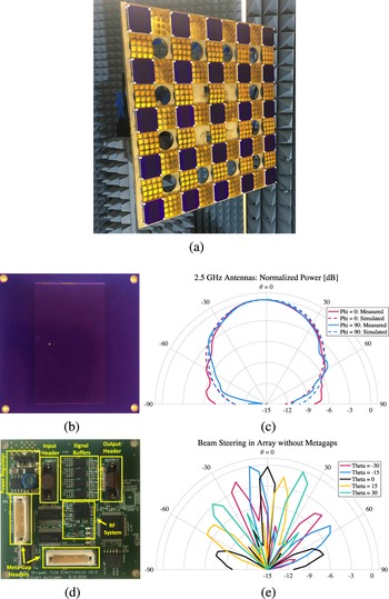
The 2.5 GHz array, shown in Figure 6(a), consists of 25 radiating tiles separated by 40 meta-gap sheets. Both the tiles and the sheets are 6 cm squares—$\frac{\lambda}{2}$ at the operating frequency—and are mounted through corner holes to nylon standoffs connected to a rigid wooden backboard. As each sheet contains 24 switches, the total array contains 960 independently programmable switches. In total, the array has 2⁹⁶⁰ different possible meta-gap configurations.

Figure 6.

(a) Demonstration array with embedded meta-gaps. (b) Tile antenna. (c) Single tile element pattern. (d) Tile electronics. (e) Measured beam patterns of array without meta-gaps.

Each tile in the array is a 2.5 GHz radiator with programmable phase and amplitude. The tiles’ RF outputs are synchronized by locking to a 78.125 MHz reference. The signal is radiated by a patch antenna on the opposite side of the tile. The patch ground-plane isolates the radiator from the electronics. Figures 6(b) and 6(d) show both sides of the tile and Figure 6(c) shows the measured and FEM-simulated radiation patterns. The simulated antenna efficiency is $84\%$.

Each tile also serves as a controller for two neighboring meta-gaps using programmable headers. Power, programming, and reference signals are distributed through the array using a single cable. To reduce the total current carried by the cables, power is distributed at 30 V and down-converted to 3.3 V by a local DC-to-DC converter on each tile.

Switched meta-gap design

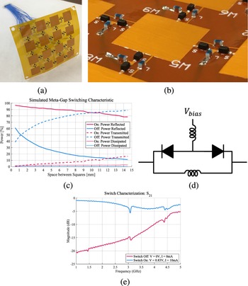
The 6-cm meta-gap sheet shown in Figure 7(a) is comprised of a 0.5-oz copper layer between two 1-mil layers of flexible polyimide. The metal forms a 4-by-4 grid of 9.7mm squares with 5.3 mm gaps. Neighboring squares are connected by an RF switch as shown in Figure 7(b). The metal grid is designed to achieve maximum variation in reflectivity and transparency when all switches are simultaneously turned on and off, respectively. When all the switches are on, the surface ideally behaves like a ground-plane, maximizing the reflection of incident waves. When all the switches are off, the surface ideally is transparent to incident waves. An FEM analysis characterizing the relationship between metal spacing and the surface’s ability to reflect incident plane waves is shown in Figure 7(c). A grid spacing of 5.3 mm is selected to minimize the power reflected when the switches are off while reflecting at least 90% of the power when the switches are on. Less than 5.5% of the incident wave power is dissipated by the structure in both the on and off states.

Figure 7.

(a) Meta-gap sheet. (b) Close-up of switching network. (c) Simulation of reflectivity and transparency versus gap size. (d) RF switch schematic. (e) Measured switch S ₂₁.

The RF switch, shown in Figure 7(d), consists of a pair of back-to-back PIN diodes biased with a 30 nH RF choke inductor. A common DC ground is established by using 30 nH inductors to connect adjacent squares. PIN diodes are used to maximize the change in switch impedance at RF frequencies and the back-to-back configuration allows an independent DC bias to be established for each switch. The measured switching behavior of the structure is shown in Figure 7(e). At 2.5 GHz, the diode insertion loss is −0.67 dB when on, and the isolation is 15.3 dB when off. Each switch is controlled with a 10 mA current via a header containing 24 control wires and 2 ground wires. The 10 mA bias current optimizes the tradeoff between insertion loss and power consumption. The lightweight 32 AWG wires are connected to the sheet from the back side. The thin substrate and wire configuration maximize sheet flexibility and minimize unwanted near-field interactions.

Measurement setup

Figure 8 is a diagram of the automated range measurement system used to perform the in-situ optimization. The demonstration array is mounted on a far-field scanner and rotated about the θ and ϕ axes. A frequency generator provides a constant 2.5 GHz signal that is converted to a 78.125 MHz reference using a pair of frequency dividers (total division ratio of 32). This reference is buffered by the array motherboard and distributed through the array under test (AUT). Each tile up-converts the reference back to 2.5 GHz, adjusts its phase, and radiates a fixed power. The combined radiated field is sensed by a horn antenna 2.95 m from the array and is measured by a vector network analyzer set to measure S ₂₁ at 2.5 GHz. This measured S ₂₁ is thus a measure of the radiated power relative to a fixed reference.

The host computer runs the metahueristic algorithms and manages the optimization and measurements by programming the array phase and meta-gap settings, controlling the scanner position, and measuring the power from the VNA. The host computer also monitors the array current, radiated spectrum, and temperature throughout the experiment to ensure reliability.

Figure 8.

Diagram of measurement setup. Blue triangles indicate RF absorbers and the boundaries of the range. Green components indicate the RF signal path. Grey squares are other critical measurement devices. Blue shapes are auxiliary equipment that monitor the measurement environment.

For MBP and SLL optimization, the array is measured by steering beams every 5^∘ from $-30^{\circ}$ to 30^∘ in the E- and H-plane cuts, while beams are steered every 5^∘ from $-90^{\circ}$ to 90^∘ for the FoV optimization. Beam steering is achieved by optimizing the tile phases to maximize power in the beam direction. For all criteria, each beam pattern is measured every 5^∘ from $-90^{\circ}$ to 90^∘ in the E- and H-plane cuts. MBP and SLL optimizations take approximately 23 h while FoV optimizations take 60.

To compensate for low frequency noise and thermal drift over the long measurement periods, each batch measures a reference state, in which every switch is turned off, and uses it to normalize the other patterns. Due to the interwoven nature of the batched measurements, different states in the batch happen in quick succession at a given measurement point; therefore, the difference between these measurements are mostly immune to low-frequency noise and temperature fluctuations. By normalizing each measured pattern to the same reference state, the relative performance of states in different batches can be accurately compared.

Figure 9.

Baseline measurements of (a), (c) main beam power and (b), (d) side lobe level in E- and H-planes for “all off” state, “all on” state, and ground-plane backed array.

Baseline measurements

While useful for measurement purposes, the “all off” state used as a baseline is not indicative of the array performance without the meta-gap sheets. A more appropriate comparison is the relative performance of the meta-gap sheet compared to a simpler approach expected to improve array performance. A reasonable solution is to fill the gaps in the array with a ground-plane, effectively creating a uniform ground-plane commonly found behind elements in an array. However, while a flexible ground-plane would make a superior baseline for comparison, it cannot be rapidly switched to electronically during an experiment.

To enable comparisons between meta-gap performance and a flexible ground-plane, the gaps in the array are filled with a ground-plane comprised of copper tape. By measuring the absolute power of the ground-plane backed array and the “all off” meta-gap state, the relative performance can be directly compared. With the relative performance of the “all off” baseline established, the performance of any meta-gap state measured relative to this baseline can be compared to the ground-plane backed array.

Figure 9 shows the MBP and SLL for the ground-plane backed array and meta-gap array in the “all on” and “all off” states normalized by the peak broadside power of the “all off” baseline. The “all on” state is included because it is the meta-gap state that corresponds with a solid ground-plane, even though the “all on” state performs worse than the copper tape ground-plane due to lossy switches and parasitic metals. The average MBP of the “all on” state is 1 dB lower than the ground-plane backed array. In general the ground-plane backed array has higher MBP and lower SLL than the meta-gap array. The only exception is the E-plane SLL which is lower when the meta-gap array is in the “all off” state.

Figure 10.

(a)–(c) Optimization curves and (d)–(f) E-plane and (g)–(i) H-plane cuts of the optimal array characteristics for the random search, genetic optimization, VNS, PS, and SA algorithms’ optimizations of main beam power, side lobe levels, and FoV under the identical sheet restriction. Optimization plots include the optimal state in addition to the value of the explored states averaged over two batches.

Identical sheet experiments

In the first set of experiments, each of the five algorithms are used to perform in-situ optimization of the MBP, the SLL, and the FoV under the restriction that each meta-gap sheet has the same switch settings. Note that unlike the statistical results in Section “Simulated Statistical Analysis,” the presented optimization results are for a single run of the experiment. Therefore, caution is warranted when drawing conclusions about the relative performance of the algorithms.

Experimental results are presented in multiple formats. Figures 10(a)–10(c) show both the algorithms’ performance over time and a moving average of the performance of states explored over two batches. This average provides another useful view of algorithm behavior. In addition, Figures 10(d)–10(i) shows the optimal array characteristic identified by each algorithm and the “all off” characteristic for each of the three optimization criteria. Finally, an illustration of the best performing meta-gap switch settings for each of the three criteria is shown in Figure 11.

Figure 11.

Visualization of optimal solution states for (a) main beam power, (b) side lobe level, and (c) field of view optimizations under the identical sheet restriction. The meta-gap sheet is represented using a four-by-four grid of light copper-colored squares separated by either black, or darker copper-colored lines. These lines indicate the status of each switch in the state; black lines indicate the switch is off while copper colored lines indicate it is on. Thus the shape of the formed conductor pattern can be visualized while still identifying the location of switches.

For both MBP and SLL, genetic optimization, PS, and SA have similar final results and outperform both VNS and random search. In both, genetic optimization identifies the best performing state, mirroring the results of the statistical experiments. When optimizing the FoV, all of the algorithms perform similarly, with PS identifying the best state.

The average value of the explored states provides additional insight. While the final MBP and SLL results of genetic optimization, PS, and SA are similar, the genetic optimization’s average state value increases much faster initially before leveling off. During this period, the algorithm quickly prunes lower performing genes. SA and PS however converge slower as they explore the full search space. The average performance of states explored by VNS oscillates as the algorithm switches between a focused local search and an unfocused perturbation to escape local optima. In the FoV optimization, however, the performance of the average state explored is similar for each of the algorithms and slowly increases over the course of the run. In all optimization criteria, the stability of the average state explored by the random search indicates long term measurement stability.

Under the identical sheet restriction, meta-gaps are able to increase the average MBP within the FoV by 1.13 dB and decrease the average SLL within the FoV by 1.7 dB when compared to the “all off” baseline. Comparing these improvements to the ground-plane measurements in Section “Baseline Measurements” indicates a 0.23 dB improvement in average MBP and a 2 dB average reduction in SLL compared to the ground-plane backed array. The performance improvement is even higher broadside; meta-gaps increase the MBP by 0.9 dB and a suppress the SLL by 4.6 dB when the beam is steered broadside.

Interestingly, even the random search is capable of suppressing the average SLL 1.3 dB more than the ground-plane backed array and improving the average MBP by at least 0.89 dB compared to the baseline, only 0.01 dB lower than the ground-plane backed antenna. Therefore it is relatively straightforward to identify meta-gap states that perform at least as well as the ground-plane backed array.

Meta-gaps are also able to increase the FoV to 83.5^∘, 23.5^∘ higher than the theoretical value of a λ spaced array. However, on examining the optimal E-plane SLL characteristic in Figure 10(f), it is clear that the FoV is improved by increasing SLL. The SLL is just barely negative for most of the expanded FoV, indicating the main lobe is only slightly higher than the peak side lobe. While this technically meets the definition of FoV, it does not follow the spirit of the concept and thus renders the results relatively impractical.Footnote ³ Nonetheless, the fact that FoV extension is even possible suggests that meta-gaps can change the aliasing behavior of the array.

Figure 11 shows the optimal meta-gap sheet switch settings for the three optimization criteria. Interestingly, the optimal MBP and SLL states are nearly identical. Both shapes suggest a split “H” shape with vertical symmetry. The optimal FoV state, however, exhibits limited symmetry with no recognizable pattern.

Symmetry experiments

The optimal states identified under the identical sheet restriction are within the larger 960 degree of freedom space and thus represent a minimum bound on the unrestricted optimal array performance. Therefore, it is possible to identify further improvements in performance by relaxing this restriction. However, this potential to increase performance comes at the cost of exponentially increasing the search space making it less likely that the algorithms can find the optimal state. Thus, there is a trade-off between the performance of the optimal state and the likelihood of identifying the state.

By considering properties that the optimal solutions are likely to have, it is possible to restrict the search space without eliminating the best performing states. It is likely that the optimal state will be symmetric due to the array symmetry. In addition, it is possible that regularity within the E- and H-planes is desirable to create a consistent near-field environment for each antenna. However, it is not clear which combination of enforced symmetries and restrictions must be true for the optimal state.

To explore the impact of different symmetries and restrictions, the MBP is optimized under seven switch mappings with different enforced symmetries and degrees of freedom. Figure 12 includes diagrams of the seven mappings; each diagram is a simplified representation of the array using a grid of squares. The degrees of freedom in each mapping ranges from 24 for the previously explored identical sheet mapping shown in Figure 12(g), to 960 for the completely unrestricted independent switch mapping shown in Figure 12(a). The remaining mappings enforce some combination of horizontal and vertical symmetry, interior sheet vs. edge sheet symmetry, or near-field symmetry. In should be noted that, except for the identical sheet mapping, the more restrictive mappings are sub-spaces of the less restrictive mappings.

Figure 12.

Diagram of mappings used to reduce degrees of freedom. The dark purple squares with arrows indicate the location and polarization of the array antennas. Black squares are the empty gaps between meta-gap sheets. Dashed lines indicate lines of enforced symmetry with mirrored switched settings across the entire array. Sheets with the same color have identical or mirrored switch settings. Each mapping is labeled by the name of the mapping and the number of degrees of freedom.

Array performance under each mapping is optimized using the SA, genetic optimization, and random search optimization algorithms. Random search is selected to establish a baseline, genetic optimization is selected due to its high performance in the identical sheet experiments, and SA is selected because it has lower variance than genetic optimization, yet still performs well. As another test, the optimal MBP states identified in the identical sheet experiments are used as initial seeds for VNS on the different mappings. By comparing the results of these different experiments, the optimal mapping is identified.

Figure 13 shows the optimization results of these experiments. For the random search, the mappings with more degrees of freedom perform worse than those that are more restricted. This is expected as the performance of the random search increases with the variability of the search space, and restricting the search space increases the electromagnetic variation between randomly selected states.

Figure 13.

Main beam power optimization curves for (a) random search, (b) genetic optimization, and (c) simulated annealing under different switch mappings. (d) Main beam power optimization curve for variable neighborhood search under different switch mappings when initialized with the best performing state identified in the identical sheet experiments. Plots include the optimal state in addition to the value of the explored states averaged over two batches.

In the genetic optimization experiment, the identical sheet restriction does not give the best results. Rather, slightly increasing the degrees of freedom with the interior vs. edge mapping and the E&H near-field mapping allows a better state to be identified. In both cases, the average state explored did not converge before the end of the experiment, indicating that a longer experiment might improve performance further. However, larger degrees of freedom degrade performance, with the independent switch mapping performing the worst.

Unlike genetic optimization, none of the mappings used in the SA experiment resulted in a better performing state than the identical sheet restriction. However the general order of the mappings’ performance is the same,Footnote ⁴ indicating that the interior vs. edge and E&H near-field mappings are indeed able to identify better solutions than the others.

The initialized VNS experiments demonstrated the same general trend; adding degrees of freedom improves performance initially before it starts to degrade. Due to the clarity of this trend, the E-plane symmetry and independent switch mappings were not explored. As can clearly be seen, the E&H near-field mapping resulted in significantly better performance than any other mapping with a 1.36 dB improvement over the baseline, or 0.46 dB improvement over a ground-plane backed array. The remarkable performance of this mapping suggests that it could be an outlier and that if the optimization was run many more times, on average the performance of this mapping would not be quite as high. However, it is unlikely that the average performance would be substantially worse than this reported result.

An important point of comparison in Figure 13(d) is the performance of the identical sheet mapping. While all of the mappings were initialized using the results of the previous identical sheet experiments, this mapping was also subject to the identical sheet restriction. This optimization thus serves effectively as an extension of the run-time of the previous identical sheet experiment. Therefore, the greater performances demonstrated by the other mappings over this second identical sheet optimization are likely due to the change in mapping, and not due to the extended run-time of the VNS algorithm.

In totality, the experiments indicate that while additional degrees of freedom can improve performance, at some point the search space is too large to find a high performing state in a reasonable amount of time. Both the interior vs. edge mapping and the E&H near-field mapping strike a balance and result in increased performance. The initialized VNS experiment indicates that the E&H near-field mapping is likely the better performing of the two.

E&H near-field experiments

In the final set of experiments, the E&H near-field mapping is thoroughly explored by optimizing the MBP, the SLL, and the FoV using each of the five optimization algorithms. As with the identical sheet experiments, the algorithms are not initialized in order to emulate the practical scenario where little is known about the array in advance.

Figure 14 shows the algorithm’s performance over time in addition to the optimal array characteristic identified by each algorithm. The similarities and differences between the Identical Sheet experiments and the E&H near-field experiments are illuminating. While genetic optimization still performs the best when optimizing the MBP and SLL, VNS outperforms SA and PS. For FoV optimization, only the VNS is able to make substantial improvements over random search; the other algorithms performed similar to, or even worse than the random search. For all of the optimization criteria, the global to local approaches are less successful as the search space increases.

Figure 14.

(a)–(c) Optimization curves and (d)–(f) E-plane and (g)–(i) H-plane cuts of the optimal array characteristics for the random search, genetic optimization, variable neighborhood search, particle swarm, and simulated annealing algorithms’ optimizations of main beam power, side lobe levels, and field of view under the E&H near-field mapping. Optimization plots include the optimal state in addition to the value of the explored states averaged over two batches.

The magnitude of the optimization results indicate that only modest improvements are gained by relaxing the identical sheet restriction. The state that maximizes the average MBP within the FoV increased it by 1.2 dB compared to the “all off” baseline, a 0.07 dB improvement over the identical sheet restriction. This corresponds to a 0.3 dB enhancement compared to the ground-plane backed array. The state that minimizes the average SLL within the FoV suppresses it by 1.7 dB compared to the baseline, the same suppression achieved by the optimal state under the identical sheet restriction. The optimal FoV identified in the E&H near-field mapping, 76.8^∘, is actually worse that the optimal FoV identified by random search in the identical sheet experiment. Thus, increasing the degrees of freedom strictly resulted in worse performance for FoV optimization. The array characteristics of the optimal state resemble those of the optimal states under the identical sheet restriction, which is not surprising given their similar performance.

The increased difficulty of the search is demonstrated by the slower convergence rates of both genetic optimization and VNS when optimizing the MBP and SLL. The average values of explored states also converge slower than in the identical sheet experiments. Indeed VNS does not begin to oscillate until over halfway through the run, indicating that it takes a long time to identify a local maxima. These convergence rates and average state performance when optimizing the FoV indicate that each of the algorithms, except VNS, essentially behave like a random search. On the other hand, VNS is able to improve performance as it quickly optimizes a local maxima if it randomly encounters one.