







1. Introduction
Initially long liquid columns always break apart into many droplets so as to minimise their surface energy. This phenomenon, referred to as Rayleigh–Plateau instability, has been well-known since the studies of Plateau (Reference Plateau1873) and Rayleigh (Reference Rayleigh1878). This instability, originally described for liquid jets, can be observed under various conditions, such as liquid film coating a fibre (Duprat Reference Duprat2009) or inside a tube (Duclaux, Clanet & Quéré Reference Duclaux, Clanet and Quéré2006), which gives rise to the formation of similar interfacial patterns and represents a class of hydrodynamic instability under the same name, reviewed in further detail in the works of Eggers & Villermaux (Reference Eggers and Villermaux2008) and Gallaire & Brun (Reference Gallaire and Brun2017). One particularly interesting variant of the Rayleigh–Plateau instability is the destabilisation of a viscous fluid draining vertically down a rigid fibre under the influence of gravity, which leads to the formation of moving beads along the fibre. This flow has been attracting attention for decades as a result of its numerous applications and rich dynamics. Some direct applications are seen in coating technologies, optical coating and drawing fibres into/from liquid baths (Quéré Reference Quéré1999; Shen et al. Reference Shen, Gleason, McKinley and Stone2002; Duprat et al. Reference Duprat, Ruyer-Quil, Kalliadasis and Giorgiutti-Dauphiné2007). Furthermore, emerging patterns are characterised mainly by a high surface area to volume ratio, which is appealing for numerous applications that involve mass and heat transfer across the liquid–gas interfaces, e.g. microfluidics (Gilet, Terwagne & Vandewalle Reference Gilet, Terwagne and Vandewalle2009), heat exchangers (Zeng et al. Reference Zeng, Sadeghpour, Warrier and Ju2017; Zeng, Sadeghpour & Ju Reference Zeng, Sadeghpour and Ju2018), vapour absorption (Chinju, Uchiyama & Mori Reference Chinju, Uchiyama and Mori2000; Grünig et al. Reference Grünig, Lyagin, Horn, Skale and Kraume2012; Hosseini et al. Reference Hosseini, Alizadeh, Fatehifar and Alizadehdakhel2014) and desalination (Sadeghpour et al. Reference Sadeghpour, Zeng, Ji, Dehdari Ebrahimi, Bertozzi and Ju2019). Predictability and control of the destabilised patterns are crucial in many of these applications.
Numerous theoretical and experimental studies have examined the flow down rigid fibres. Remarkably, Kliakhandler, Davis & Bankoff (Reference Kliakhandler, Davis and Bankoff2001) reported experimentally three distinct unstable regimes: (i) isolated beads, (ii) regularly distanced beads train, and (iii) irregularly distanced beads train. Transition from the absolute to convective regimes occurs when the film thickness exceeds a critical value, for which the corresponding thresholds are discussed widely in the works of Chang & Demekhin (Reference Chang and Demekhin1999) and Duprat et al. (Reference Duprat, Ruyer-Quil, Kalliadasis and Giorgiutti-Dauphiné2007). Besides secondary instabilities and nonlinear phenomena that may be observed as beads grow, solitary waves may appear along the fibre in the non-zero inertia limit, reminiscent of the capillary Kapitza waves (Kapitza Reference Kapitza1965; Duprat Reference Duprat2009). Several theoretical and numerical models have been proposed to elucidate the dynamics of the growth and motion of the emergent unstable patterns in the linear and nonlinear regimes in the limits of thin film (Frenkel Reference Frenkel1992; Ruyer-Quil et al. Reference Ruyer-Quil, Treveleyan, Giorgiutti-Dauphiné, Duprat and Kalliadasis2008; Ruyer-Quil & Kalliadasis Reference Ruyer-Quil and Kalliadasis2012; Yu & Hinch Reference Yu and Hinch2013) and thick film (Craster & Matar Reference Craster and Matar2006; Liu & Ding Reference Liu and Ding2021). Each of these models captures some features of the destabilisation process and matches the experimental data within some ranges. In addition, further studies concluded that besides the liquid properties, the fibre properties such as porosity (Ding & Liu Reference Ding and Liu2011), slip properties (Haefner et al. Reference Haefner, Benzaquen, Bäumchen, Salez, Peters, McGraw, Jacobs, Raphaël and Dalnoki-Veress2015) and shape (Xie et al. Reference Xie, Liu, Wang and Chen2021), as well as geometric parameters like nozzle geometry (Sadeghpour, Zeng & Ju Reference Sadeghpour, Zeng and Ju2017), have significant impacts on altering the dynamics and defining the range of occurrence of each unstable regime. Changes to the dynamics may be related to changing the dominant wavelength, switching between different regimes, and changing the spacing, velocity, shape and coalescence of mobile beads.
In all of the studies in the literature, the fibre is concentric with the liquid column, and the initial stage of any unstable regime exhibits an axisymmetric growth of the interface undulations. The recent work of Gabbard & Bostwick (Reference Gabbard and Bostwick2021) addresses the evolution of asymmetric beads when the film thickness is initially non-homogeneous around the fibre. In their case, they outlined the thresholds between the three regimes of isolated beads, and regular and irregular beads trains. Yet a full understanding of the destabilisation processes is missing for the stability of non-homogeneous film thickness in flows down a fibre. For instance, it is not clear why the formation of asymmetric beads is not prevented by capillary effects. Also, the effect of non-homogeneous film thickness on the linear instability of other non-axisymmetric modes is not known. In the present study, we focus on the effect of the fibre position with respect to the liquid column, and we investigate the stability characteristics of the flow and the subsequent geometry of the emerging patterns.
This paper is structured as follows. The methodology is first presented in § 2. To begin with, the problem formulation and the governing equations are presented in § 2.1, from which the base flow is deduced and discussed in § 2.2. In § 2.3, the stability analysis formulation and the linearised governing equations are elaborated. Corresponding numerical methods are detailed in § 2.4. In § 3, the results of the stability analyses are presented and discussed. First, in § 3.1, the effect of the fibre eccentricity on the stability characteristics of the flow is given. Then a similar investigation is conducted for the other dimensionless parameters in §3.2, followed by sketching the extensive stability maps in § 3.3. In addition, the physical mechanisms underlying the instability of the flow are elucidated by the method of energy analysis in § 3.4. In § 3.5, a comparison between the linear model and our illustrative experiments is provided. Finally, conclusions are drawn in § 4.
2. Governing equations and methods
2.1. Problem formulation
A viscous liquid column flows under gravity along a vertical solid cylindrical fibre of radius  $R_{f}$ placed with eccentricity $r_{{ec}}$ from the centre of the column. The schematic of the flow and the cross-sectional view are shown in figure 1. The standard Cartesian coordinates $(x,y,z)$ are considered, with the origin located at the centre of the liquid column. In-plane coordinates are $(x,y)$, and the positive direction of the axial/vertical coordinate $z$ points in the direction of the gravity acceleration $g$. The liquid is Newtonian, of constant dynamic viscosity $\mu$, surface tension $\gamma$ and density $\rho$, and is surrounded by an inviscid gas. Without loss of generality for sufficiently small interface deformations, the interface can be parametrised in cylindrical coordinates $(r,\theta,z)$ as $r_{int}(t,\theta,z)$, using the same origin as the Cartesian one, and $R$ denotes the reference value of $r_{int}$ in the absence of any perturbation. The dimensionless state vector $\boldsymbol {q}= (\boldsymbol {u},p,R_{int})^{{\rm T}}$ defines the flow where at time $t$,
$t$,  $\boldsymbol {u}(t,x,y,z)= (u_x,u_y,u_z)^{{\rm T}}$ denotes the three-dimensional velocity field, $p(t,x,y,z)$ denotes the pressure, and $R_{int}=r_{int} / R$ denotes the dimensionless interface radius. As opposed to Craster & Matar (Reference Craster and Matar2006), the state vector and the governing equations are rendered dimensionless by the intrinsic velocity and time scales presented by Duprat (Reference Duprat2009), associated with the viscous axisymmetric liquid ring of uniform thickness $h_0=R-R_{f}$ that coats a centred fibre. However, we choose different length and pressure scales, as follows:
 \begin{equation} \left.\begin{gathered} \mathcal{L}=R,\quad \mathcal{U}=\frac{\rho g h_0^2}{\mu}=\frac{\rho g R^2}{\mu}\,(1-\alpha)^2,\\ \mathcal{P}=\rho g R,\quad \mathcal{T}=\frac{\mathcal{L}}{\mathcal{U}}= \frac{\mu}{\rho g R}\,(1-\alpha)^{{-}2}, \end{gathered}\right\} \end{equation}
where  $\alpha = {R_{f}}/{R}$ denotes the fibre to mean radius aspect ratio. The other geometric parameter is $R_{ec}= {r_{ec}}/{R}$, which denotes the dimensionless fibre eccentricity. The flow is governed by the incompressible Navier–Stokes equations, which in dimensionless form read
 $$\begin{gather} \boldsymbol{\nabla}\boldsymbol{\cdot} \boldsymbol{u}=0, \end{gather}$$
 $$\begin{gather}\frac{Bo}{Oh^2}\,(1-\alpha)^4 ( {\partial}_t + {\boldsymbol{u}}\boldsymbol{\cdot}\boldsymbol{\nabla} )\boldsymbol{u} =\boldsymbol{\nabla}\boldsymbol{\cdot} \underline{\underline{{\tau}}} +1 \boldsymbol{e}_z, \end{gather}$$
where  $ {\partial }_j$ denotes the partial derivative with respect to quantity $j$, and the stress tensor $\underline {\underline {\tau }}$ reads
 \begin{equation} \underline{\underline{{\tau}}}={-}{p} \boldsymbol{\mathsf{I}} + (1-\alpha)^2 \left(\boldsymbol{\nabla} {\boldsymbol{u}} + \boldsymbol{\nabla} {\boldsymbol{u}}^{{\rm T}} \right). \end{equation}
The two other dimensionless numbers that appear in the governing equations are the Ohnesorge number  $Oh={\mu }/{\sqrt {\rho \gamma R}}$, and the Bond number $Bo={\rho g R^2}/{\gamma }$. While $Oh$ compares the viscous forces to the inertial and surface tension forces, $Bo$ compares the gravitational and surface tension forces. Our study addresses the limit of inertialess flow where $({Bo}/{Oh^2}) (1-\alpha )^4 \ll 1$ without any further assumptions on $\alpha$.
Schematic of the coating flow along an eccentric fibre and the geometrical parameters in cross-sectional view. The outer dashed black line represents the perturbed interface of local radius  $r_{int}$ and axial wavelength $R \lambda$, and the outer solid black line shows the cylinder with mean radius $R$, which is concentric with the coordinate reference. The planar cut shows the cross-section of the liquid column and the geometrical characteristics, where the grey region shows the solid fibre.

The no-slip boundary condition  $\boldsymbol {u} = 0$ is applied on the fibre $ {\partial } \varSigma _{{f}}$. On the shear-free fluid–gas interface, the kinematic and dynamic boundary conditions, respectively, are
 $$\begin{gather} {\partial}_t R_{int} + \boldsymbol{u} \boldsymbol{\cdot}\boldsymbol{\nabla} R_{int}= \boldsymbol{u}\boldsymbol{\cdot} \boldsymbol{e}_r \quad \text{on}\ r=R_{int}, \end{gather}$$
 $$\begin{gather}\underline{\underline{{\tau}}}\,{\boldsymbol{n}} ={-} \frac{\kappa}{Bo}\, {\boldsymbol{n}} \quad \text{on}\ r=R_{int}, \end{gather}$$
where  $\boldsymbol {e}_r$ denotes the unit radial vector, $\boldsymbol {n} = \boldsymbol {\nabla } ( r-R_{int}) / \Vert \boldsymbol {\nabla } (r-R_{int})\Vert$ denotes the unit normal vector pointing outwards from the liquid bulk, $\Vert \cdot \Vert$ denotes the Euclidean norm, and $\kappa =\boldsymbol {\nabla } \boldsymbol {\cdot }{\boldsymbol {n}}$ denotes the interface mean curvature.
2.2. Base flow
The base flow  $\boldsymbol {q}^0$ is the steady-state solution of the Navier–Stokes equations (2.2)–(2.6). We recall the solution prevailing for an eccentric fibre. In the limit of a centred fibre, the analytical solution exists whose axial velocity is composed of a logarithmic term and a parabola as
 \begin{equation} u^0_z= \frac{(1-\alpha)^{{-}2}}{2} \left( \ln{\frac{r}{\alpha}} - \frac{r^2-\alpha^2}{2} \right),\quad p^0 = \frac{1}{Bo}, \end{equation}
with a constant pressure in the liquid. This velocity field is shown in figure 2(a) and reveals its maximal velocity at the liquid–gas interface, and an increasing drainage flux  $Q^0=\iint _{\varOmega _{xy}} u^0_z \,\mathrm {d}A_{\varOmega _{xy}}$ as the aspect ratio $\alpha$ decreases, i.e. for a thicker liquid film (figure 2b). Inspired by the solution for the centred fibre, we seek a base flow that is parallel and fully developed in the $z$ direction with a cylindrical interface of radius $R^0_{int}=1$. Note that $R^0_{int}=1$ is readily a solution to the nonlinear kinematic condition (2.5). Assuming a constant pressure, the normal component of the dynamic condition (2.6) is also satisfied. It remains to solve the Poisson equation for $u^0_z$, with no-slip on the fibre and free shear on the interface, driven by gravity. The solution is computed numerically in the present study (see § 2.4 for details) for the flow coating an eccentric fibre, although it could be interesting to try to extend to the present free-surface configuration the method proposed in Piercy, Hooper & Winney (Reference Piercy, Hooper and Winney1933) for a pipe flow with a solid core. The fibre eccentricity breaks the axisymmetry of the base flow, with a high-speed region on the thicker side of the liquid film, and a low-speed region on the thinner side. On the thicker side, shear is decreased near the interface while being increased in the vicinity of the fibre (solid lines in figure 2c); on the thinner side, it evidences an increase near the interface while being decreased near the fibre (dashed lines in figure 2c). The drainage flow rate increases substantially with $R_{ec}$ (figure 2b).
Variation of the base flow as a result of the fibre eccentricity. (a) Axial velocity  $u^0_z$ at the cross-section for $\alpha =0.1$ and three different values of fibre eccentricities $R_{ec}=0,0.1,0.5$; same colour bar applies for all plots. (b) Vertical flow rate $Q^0$ for different values of $\alpha$ and $R_{ec}$; solid black lines show the results from our numerical study, and the red dots show the values computed from the analytical flow around a centred fibre, (2.7a,b); for each value of $\alpha$, the plot stops at $\alpha + R_{ec} \leq 0.95$; (c) Shear rate across the thick (continuous) and thin (dashed) sides of the liquid film along $y=0$.

2.3. Linear stability analysis
In order to perform the linear stability analysis on the base flow, presented in § 2.2, the state vector  $\boldsymbol {q}= (\boldsymbol {u},p,R_{int})^{\textrm {T}}$ is decomposed into the sum of the steady-state base flow solution $\boldsymbol {q}^0$, and the infinitesimal time-dependent perturbation $\boldsymbol {q}^1= (\boldsymbol {u}^1,p^1,\eta ^1 )^{\textrm {T}}$, i.e.
 \begin{equation} \boldsymbol{q}=\boldsymbol{q}^0 + \epsilon \boldsymbol{q}^1 + {O}(\epsilon^2),\quad \epsilon \ll 1, \end{equation}
where the amplitude  $\epsilon$ is assumed to be small. We look for perturbations $\boldsymbol {q}^1$ under the normal form
 \begin{equation} \boldsymbol{q}^1=\tilde{\boldsymbol{q}}(x,y) \exp [ \sigma t+\mathrm{i}kz ] + \mathrm{c.c.}, \end{equation}
with  $k$ being the longitudinal wavenumber (associated with the wavelength $\lambda ={2 {\rm \pi}}/{k}$), and c.c. denoting the complex conjugate. It should be noted that the eccentricity of the fibre breaks the axisymmetry of the problem, in spite of a cylindrical base interface. Therefore, a normal mode of the form $\tilde {\boldsymbol {q}}(r) \exp [ \sigma t+\mathrm {i}m \theta + \mathrm {i}kz ] + \mathrm {c.c.}$, with $m$ being the azimuthal wavenumber, is not suitable in the eccentric configuration. In the asymptotic limit of large times, a normal eigenmode perturbation with complex pulsation $\sigma =\sigma _r + \mathrm {i} \sigma _i$ is defined as unstable and hence grows exponentially in time with the growth rate $\sigma _r$, if $\sigma _r > 0$, i.e. if $\sigma$ is in the unstable complex half-plane. (Unless otherwise noted, the subscripts $r$ and $i$ denote the real and imaginary parts of a complex number, respectively.) By casting the perturbed state of (2.8) into the governing equations (2.2)–(2.3), with the stationary base flow $\boldsymbol {q}^{0}=(\boldsymbol {u}^0,{1}/{Bo},1)^{\textrm {T}}$, and keeping the first-order terms, the linearised equations are obtained as
 $$\begin{gather} \boldsymbol{\nabla}\boldsymbol{\cdot}\boldsymbol{u}^1=0, \end{gather}$$
 $$\begin{gather}\frac{Bo}{Oh^2} (1-\alpha)^4 ({\partial}_t \boldsymbol{u}^1 + (\boldsymbol{u}^0 \boldsymbol{\cdot}\boldsymbol{\nabla}) \boldsymbol{u}^1 + (\boldsymbol{u}^1 \boldsymbol{\cdot}\boldsymbol{\nabla}) \boldsymbol{u}^0 ) = \boldsymbol{\nabla}\boldsymbol{\cdot}\underline{\underline{\tau}}^1. \end{gather}$$
 The no-slip condition implies  $\tilde {\boldsymbol {u}}=0$ on the fibre. The perturbed interface boundary conditions (2.5)–(2.6), applied on the perturbed liquid interface, can be projected radially onto the base interface and ultimately linearised, a process called flattening (see (A1) in Appendix A). The linearised kinematic condition can be expressed as
 \begin{equation} ( \sigma + \mathrm{i} k u_{z}^0 ) \tilde{\eta} = \tilde{\boldsymbol{u}} \boldsymbol{\cdot}\boldsymbol{e}_r \quad \text{on}\ r=1. \end{equation}
Introducing an eigenstate vector of the form (2.9) into (2.10)–(2.11), combined with (2.12), leads to a generalised eigenvalue problem for  $\sigma$ and $\tilde {\boldsymbol {q}}$:
 \begin{equation} \boldsymbol{\mathsf{L}} \tilde{\boldsymbol{q}} + \text{c.c.} = \sigma \boldsymbol{\mathsf{B}} \tilde{\boldsymbol{q}} + \text{c.c.}, \end{equation}
where the linear operators  $\boldsymbol{\mathsf{L}}$ and $\boldsymbol{\mathsf{B}}$ are defined as
 \begin{align}
\boldsymbol{\mathsf{L}}= \begin{bmatrix} (1-\alpha)^2
\left( \widetilde{\boldsymbol{\nabla}}\boldsymbol{\cdot}
(\widetilde{\boldsymbol{\nabla}}+\widetilde{\boldsymbol{\nabla}}^{{\rm
T}}) \right) & -\widetilde{\boldsymbol{\nabla}} &
\boldsymbol{0} \\
\widetilde{\boldsymbol{\nabla}}\boldsymbol{\cdot} & 0 & 0
\\ \boldsymbol{e}_r & 0 & - \mathrm{i} k u_{z}^0
\end{bmatrix},\quad \boldsymbol{\mathsf{B}} =
\begin{bmatrix} \dfrac{Bo}{Oh^2}\,(1-\alpha)^4
\boldsymbol{\mathsf{I}} & \boldsymbol{0} &
\boldsymbol{0} \\ \boldsymbol{0} & 0 & 0 \\ \boldsymbol{0}
& 0 & 1 \, \end{bmatrix}, \end{align}
\begin{align}
\boldsymbol{\mathsf{L}}= \begin{bmatrix} (1-\alpha)^2
\left( \widetilde{\boldsymbol{\nabla}}\boldsymbol{\cdot}
(\widetilde{\boldsymbol{\nabla}}+\widetilde{\boldsymbol{\nabla}}^{{\rm
T}}) \right) & -\widetilde{\boldsymbol{\nabla}} &
\boldsymbol{0} \\
\widetilde{\boldsymbol{\nabla}}\boldsymbol{\cdot} & 0 & 0
\\ \boldsymbol{e}_r & 0 & - \mathrm{i} k u_{z}^0
\end{bmatrix},\quad \boldsymbol{\mathsf{B}} =
\begin{bmatrix} \dfrac{Bo}{Oh^2}\,(1-\alpha)^4
\boldsymbol{\mathsf{I}} & \boldsymbol{0} &
\boldsymbol{0} \\ \boldsymbol{0} & 0 & 0 \\ \boldsymbol{0}
& 0 & 1 \, \end{bmatrix}, \end{align}
and the gradient operator and the velocity gradient tensor in Cartesian coordinates are
 \begin{equation} \widetilde{\boldsymbol{\nabla}} = ({\partial}_x, {\partial}_y,\mathrm{i}k)^{{\rm T}},\quad \widetilde{\boldsymbol{\nabla}} \widetilde{\boldsymbol{u}} = \begin{bmatrix} {\partial}_x \tilde{u}_x & {\partial}_y \tilde{u}_x & \mathrm{i}k \tilde{u}_x \\ {\partial}_x \tilde{u}_{y} & {\partial}_y \tilde{u}_{y} & \mathrm{i}k \tilde{u}_{y} \\ {\partial}_x \tilde{u}_z & {\partial}_y \tilde{u}_z & \mathrm{i}k \tilde{u}_z \, \end{bmatrix}. \end{equation}
The operators  $\boldsymbol{\mathsf{L}}$ and $\boldsymbol{\mathsf{B}}$ are then modified to enforce the dynamic condition, which can be expressed as
 \begin{align} \underline{\underline{{\tilde{\tau}}}} {\boldsymbol{n}}^0 &={-} \frac{\tilde{\kappa}}{Bo}\,\boldsymbol{e}_r \nonumber\\ &\quad + (1-\alpha)^2\,{\partial}_{\theta} u^0_z\,\mathrm{i}k \tilde{\eta} \boldsymbol{e }_{\theta} \nonumber\\ &\quad + (1-\alpha)^2 ({\partial}_{\theta} u^0_z\,{\partial}_{\theta} \tilde{\eta} - {\partial}_{rr} u^0_z \tilde{\eta}) \boldsymbol{e}_z \quad \text{on}\ r=1, \end{align}
where  $\tilde {\kappa }$ denotes the dimensionless curvature perturbation expressed as
 \begin{equation} \tilde{\kappa} = ( k^2-1 )\tilde{\eta} - \frac{{\partial}^2 \tilde{\eta}}{{\partial} \theta^2}, \end{equation}
and  $(\boldsymbol {e}_r,\boldsymbol {e}_{\theta },\boldsymbol {e}_z)$ denote the unit vectors of directions in the cylindrical coordinates $(r,\theta,z)$ used for parametrising the interface; see figure 1. (For further details on the interface boundary conditions’ derivation and implementation, see Appendix A and § B.2, respectively.)
2.4. Numerical method
The base flow and linear stability analysis are solved numerically with the finite element method. We use the software COMSOL Multiphysics. A triangular mesh of the two-dimensional domain, shown in figure 3, is generated with the Delaunay–Voronoi algorithm. The grid size is controlled by the vertex densities on the boundaries  $ {\partial } \varSigma _{{f}}$ and $ {\partial } \varSigma _{{int}}$. The variational formulation of the base flow equations (2.2)–(2.6) and the linear stability equation (2.13) are discretised spatially using quadratic (P2) Lagrange elements for $\boldsymbol {u}^0$, $\widetilde {\boldsymbol {u}}$ and $\tilde {\eta }$, and linear (P1) Lagrange elements for $\tilde {p}$, yielding approximately 200 000 and 700 000 degrees of freedom for the base flow and the linear stability analysis, respectively. The base flow, the solution of a linear Poisson equation, is computed first with a linear solver. Then this base flow is used to solve the generalised eigenvalue problem associated with the linear stability analysis using a shift-invert Arnoldi method. (See Appendix B for details about the variational formulations and corresponding boundary conditions, and their implementation.)
The numerical domain used for computing the base flow and linear stability analysis; the outer radius of the domain is set to unity, the same as that of the base interface. Here,  $\varOmega _{xy}$ denotes the liquid bulk. The boundaries of the numerical domain are denoted by $ {\partial } \varOmega _{xy} = {\partial } \varSigma _{{f}} \cup {\partial } \varSigma _{{int}}$, where $ {\partial } \varSigma _{{f}}$ represents the liquid–fibre contact boundary, and $ {\partial } \varSigma _{{int}}$ represents the gas–liquid interface.

The computation time associated with one given set of variables, followed by the stability analysis for  $\sim$20 values of $k$, is of the order of tens of minutes on a single Intel core at 3.6 GHz. The model is validated with the analytical solutions in the literature for the coating flow over a centred fibre. (For more details about the series of validation tests, see Appendix C.)
3. Results
3.1. Effect of the fibre eccentricity ( $R_{ec}$)

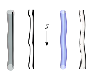
The results of the linear stability analysis are presented hereafter. Figure 4 shows the effect of  $R_{ec}$ on the stability of the flow. The dispersion curve, $\sigma _r$ versus $k$, is plotted in figure 4(a) for the two least linearly stable eigenmodes, which can be characterised by the shapes of their eigeninterfaces in figures 4(b,c). In the limit of the concentric fibre, $R_{ec}=0$, only one unstable mode exists in the range $0 < k \leq 1$, which undulates axisymmetrically in the axial direction. This instability is known as a variant of the Rayleigh–Plateau instability (Rayleigh Reference Rayleigh1878). The second mode is stable over the whole range of wavenumbers, and its interface forms a single helix that whirls along the axial direction. Accordingly, hereafter, we will refer to these two modes as the pearl (P) and whirl (W) modes, respectively. We emphasise that this instability is not to be confused with the classical whirl instability observed in liquid/gas-lubricated journal bearings, that is, a self-excited rotor whirl caused by lubricating film forces when the rotation frequency of the shaft exceeds a threshold, approaching the lowest natural frequency of the system (Harrison Reference Harrison1912; Larson & Richardson Reference Larson and Richardson1962).
Evolution of the two least stable eigenmodes, P (black) and W (blue), with increasing fibre eccentricity, plotted for  $R_{ec}=0,0.1,0.5$. (a) The dispersion curve. (b) A three-dimensional render of the perturbed interface obtained by superposition of the real part of the corresponding eigeninterfaces with amplitude 20 $\%$ onto the base interface over an axial span of double wavelength $r(\theta,z)=1+0.2\tilde {\eta }_r \cos (kz)$. (c) Real part of the eigeninterface, $\tilde {\eta }_r$, as a function of $\theta$. All of the plots correspond to $Oh \rightarrow \infty$, $Bo=50$ and $\alpha =0.1$, and the eigeninterfaces are plotted at $k=0.1$. All of the eigenstates are normalised and presented in the same complex phase, such that at the maximal positive interface perturbation, $\tilde {\eta }=1$.

By increasing  $R_{ec}$, the general trend observed in the stability of these two modes is as follows. The eigeninterfaces of both modes are deformed as the flow symmetry breaks, but their general layout remains similar to that of the concentric fibre. In addition, the P mode remains unstable, although its dispersion curve exhibits an alteration of the range of unstable wavenumbers. Moreover, increasing $R_{ec}$ over a certain threshold destabilises the W mode, and by increasing $R_{ec}$ further, the W mode eventually dominates over the P mode in a range of wavenumbers.
3.2. $Bo$ and $\alpha$ effects


In this subsection, the effects of  $Bo$ and $\alpha$ on the stability characteristics of the flow are illustrated via dispersion curves. Figure 5(a) highlights the main changes induced by decreasing $\alpha$. The instability range of the P mode extends. Additionally, although the maximal growth rate of the P mode exhibits a minor change, its maximal wavenumber – i.e. the wavenumber at which the maximal growth rate occurs – increases. Moreover, reducing $\alpha$ to less than a certain threshold destabilises the W mode. By further reducing $\alpha$, the maximal wavenumber of the W mode and its growth rate increase, and eventually its growth rate dominates that of the P mode in some range of wavenumbers. Similar to decreasing $\alpha$, figure 5(b) demonstrates the effects of increasing $Bo$ as destabilising the W mode until its dominance over the P mode. Besides, larger $Bo$ increases the instability range of both P and W modes. Unlike the W mode, the maximal growth rate of the P mode decreases by increasing $Bo$.
$Bo$.
Variation of dispersion curve for the P (black) and W (blue) modes. (a) The  $\alpha$ effect, plotted for $Oh \rightarrow \infty$, $Bo=50$, $R_{ec}=0.3$ and $\alpha =0.1,0.15,0.3$; each arrow shows the direction of increasing $\alpha$ for the P mode dispersion curve. (b) The $Bo$ effect, plotted for $Oh\rightarrow \infty$, $R_{ec}=0.7$, $\alpha =0.1$ and $Bo=4,5,6,10$; each arrow shows the direction of increasing $Bo$ for the P mode dispersion curve.

So far, three principal unstable regimes are identified in the parameter space: (i) only the P mode is unstable; (ii) both P and W modes are unstable, and the P mode dominates; (iii) both P and W modes are unstable, and the W mode dominates. A detailed study of the parameter space is conducted, and the results are presented in § 3.3.
3.3. Phase diagrams
The  $\{Bo,\alpha,R_{ec}\}$ space is investigated extensively to determine the threshold of the unstable regimes. Figures 6(a,b) present the phase diagrams that are obtained by holding $\alpha$ and $Bo$ fixed, respectively, while varying the other parameters. For any set in the investigated range of parameters, the P mode destabilises. Furthermore, in accordance with the results presented in §§ 3.1 and 3.2, these diagrams show that exceeding a certain threshold, increasing $Bo$ for a fixed $\{ \alpha,R_{ec} \}$, or decreasing $\alpha$ for a fixed $\{Bo,R_{ec} \}$, leads to the coexistence of unstable P and W modes, first with the dominance of the P mode, and later the dominance of the W mode. For instance, figure 6(b) reveals that at a constant $Bo=50$, there are two cut-off values of $R_{ec}$: first, below $R_{ec} \approx 0.28$, the W mode never dominates the P mode for a finite fibre size; second, below $R_{ec} \approx 0.2$, only the P mode destabilises. Figure 6(b) is limited to $\alpha \ge 0.075$ for numerical reasons, that is, the appearance of spurious eigenmodes with discontinuities in the interface perturbation $\tilde {\eta }$ for $\alpha \le 0.05$. Mesh refinement on the fibre boundary, on the interface boundary and inside the domain did not resolve this numerical issue.
Phase diagrams of the unstable modes associated with the gravity-driven coating flow along an eccentric fibre: (a) for  $\alpha =0.1$, $Oh \rightarrow \infty$; (b) for $Bo=50$, $Oh\rightarrow \infty$. The dotted curves mark the interpolated thresholds obtained from numerical eigenvalue calculations. The grey region in the right-hand corner excludes the infeasible geometrical limit $\alpha + R_{ec} \geq 1$ where the fibre touches the base interface. The coloured regions indicate the instabilities and dominance in terms of the growth rate as follows: white means only the P mode destabilises; red means both P and W modes destabilise, and P dominates; blue means both P and W modes destabilise, and W dominates.

Formerly, extensive studies addressed the shapes of the pearls in contact with a fibre (Carroll Reference Carroll1984; Brochard-Wyart, Di Meglio & Quéré Reference Brochard-Wyart, Di Meglio and Quéré1990; McHale et al. Reference McHale, Rowan, Newton and Käb1999; McHale, Newton & Carroll Reference McHale, Newton and Carroll2001; Duprat Reference Duprat2009). However, instability of the W mode is not expected, as Rayleigh (Reference Rayleigh1878) states that any non-axisymmetric perturbation should be linearly stable. The reason is that the surface energy of a liquid column is proportional to its surface area, which increases with the formation of whirling structures. Hence, such patterns are not in favour of the surface energy minimisation and should not destabilise (Cardoso & Dias Reference Cardoso and Dias2006; Duprat Reference Duprat2009; Gallaire & Brun Reference Gallaire and Brun2017). Moreover, even though some studies have addressed the linear instability of the helical mode in the context of interfacial columnar flows, in each case an extra physical mechanism causes helical instability. For instance, aerodynamic interactions at the interface of inertial jets (Yang Reference Yang1992), elasticity and electric stresses at the interface of electrified jets (Li, Yin & Yin Reference Li, Yin and Yin2011), and the solid–liquid–gas contact line at the interface of static rivulets (Bostwick & Steen Reference Bostwick and Steen2018) are at play to counteract capillarity, promoting helical instabilities. In our study, i.e. in the absence of these extra triggering mechanisms, capillarity is known to stabilise non-axisymmetric interface perturbations. This apparent paradox gives the motivation to § 3.4, where we perform an energy analysis on the flow.
3.4. Energy analysis
In this subsection, in an attempt to clarify the competition between capillary, potential and viscous effects, and to quantify their respective contributions to the base flow and the stability of modes P and W, we study the flow from an energy perspective. The base flow presented in § 2.2, and the perturbed flow resulting from the linear stability analysis and presented in §§ 3.1–3.2, are investigated by means of the method of energy analysis to explain the underlying physics of the flow instability. Previously, Boomkamp & Miesen (Reference Boomkamp and Miesen1996), Hooper & Boyd (Reference Hooper and Boyd1983), Kataoka & Troian (Reference Kataoka and Troian1997) and Li et al. (Reference Li, Yin and Yin2011) employed this method to determine and compare the roles of different physical mechanisms on the temporal instability of various interfacial flows.
In the following sections, the area increment in the bulk cross-section is denoted by  $\mathrm {d} \boldsymbol{A}_{\varOmega _{xy}}$. On the boundary $j$, the increment of surface area is denoted by $\mathrm {d} \boldsymbol{A}_{\varSigma _j}$, and the increment of arc length is denoted by $\mathrm {d} s$. What is commonly referred to as the energy analysis is in fact the study of the energy conservation in a flow, in different scales, from the base flow to the perturbations. More precisely, this analysis sheds light on the rate of energy balance equation, hereafter referred to as the energy equation, which for the inertialess gravity-driven flow along a fibre can be expressed as
 \begin{equation} \underbrace{\iiint_{\varOmega_{xy}} (1-\alpha)^2\,{\rm tr}\left((\boldsymbol{\nabla} \boldsymbol{u} + \boldsymbol{\nabla}^{{\rm T}} \boldsymbol{u} ) \boldsymbol{\nabla} \boldsymbol{u }\right)}_{\text{DIS}} + \underbrace{\iint_{{\partial} \varSigma_{{int}}} -\left(\underline{\underline{{\tau}}} \boldsymbol{n}^0 \right) \boldsymbol{\cdot} \boldsymbol{u}}_{\text{BND}} + \underbrace{\iiint_{\varOmega_{xy}} - u_z}_{\text{POT}} = 0, \end{equation}
where the bulk integrals are defined on the volume increment  $\mathrm {d} V=\mathrm {d} A_{\varOmega _{xy}}\,\mathrm {d} z$, the surface integral is defined on the cylindrical surface with cross-section $ {\partial } \varSigma _{{int}}$ and axis in the $z$ direction (see figure 3), DIS denotes the rate of viscous dissipation in the bulk fluid, BND denotes the rate of work done by the fluid through the interface, and POT denotes the rate of change of gravitational potential energy. (For more details about the derivation of the energy equation and its non-simplified and dimensional form, see Appendix D.) The energy equation implies that the energy is released and consumed in the flow at the same rates, whereas multiple physical mechanisms may contribute to its release and consumption. In this regard, the sign of each term in (3.1) indicates whether the energy is removed from ( $+$) or released into ( $-$) the flow by the respective mechanism.
3.4.1. Energy analysis of the base flow
The energy equation for the base flow presented in § 2.2, computed per unit length in  $z$, can be expressed by
 \begin{equation} \underbrace{\iint_{\varOmega_{xy}} (1-\alpha)^2\,{\rm tr}\left({(\boldsymbol{\nabla} \boldsymbol{u}^0 + \boldsymbol{\nabla}^{{\rm T}} \boldsymbol{u}^0 ) \boldsymbol{\nabla} \boldsymbol{u}^0 } \right)}_{\text{DIS}^0} + \underbrace{\iint_{\varOmega_{xy}} - {u}_z^0 }_{\text{POT}^0={-}Q^0} = 0, \end{equation}
which demonstrates that the potential energy released in the flow by drainage of the liquid is steadily dissipated in the bulk liquid. We recall that  $Q^0>0$ (see figure 2) and the rate of potential energy release increases by increasing $R_{ec}$. Furthermore, recalling the dynamic condition (2.6), BND $^0=0$, which means that no energy is exchanged with the base flow from the cylindrical interface.
3.4.2. Energy analysis of the perturbed flow
The energy equation at the scale of the linear perturbations, i.e.  $\epsilon ^2$, computed along one wavelength, implies
 \begin{align} & \left(\underbrace{\iint_{\varOmega_{xy}} (1-\alpha)^2\,{\rm tr}\left({(\widetilde{\boldsymbol{\nabla}} \widetilde{\boldsymbol{u}} + \widetilde{\boldsymbol{\nabla}}^{{\rm T}} \widetilde{\boldsymbol{u}}) \widetilde{\boldsymbol{\nabla}} \widetilde{\boldsymbol{u}}^\star}\right)}_{\text{DIS}^1}\right)_r \nonumber\\ &\quad + \left(\underbrace{\int_{{\partial} \varSigma_{{int}}} \frac{{\sigma}^\star}{Bo}\, \tilde{\kappa} \tilde{\eta}^\star}_{{\text{BND}^1_{c,1}} = {\sigma}^\star \text{SUR}^1} + \underbrace{\int_{{\partial} \varSigma_{{int}}}\frac{-\mathrm{i} k u^0_z}{Bo}\, \tilde{\kappa} \tilde{\eta}^\star}_{\text{BND}^1_{c,2}} + \underbrace{\int_{{\partial} \varSigma_{{int}} } -\left(\underline{\underline{\tilde{\tau}_{v}}} \boldsymbol{n}^0 \right) \boldsymbol{\cdot} \widetilde{\boldsymbol{u}}^\star}_{\text{BND}^1_{v}}\right)_r =0, \end{align}
where  $\star$ denotes the complex conjugate, ${\textrm {BND}^1_{c,1}}$ and $\textrm {BND}^1_{c,2}$ denote the capillary contributions to the rate of the work done by the fluid at the perturbed interface, $\textrm {SUR}^1$ denotes the surface energy stored in the perturbed interface, $\underline {\underline {\tilde {\tau }_{v}}}$ denotes the viscous contribution of the stress tensor, and $\textrm {BND}^1_{v}$ denotes the viscous (shear) contribution to the rate of the work done by the fluid at the perturbed interface, which can be expressed as
 \begin{align} \text{BND}^1_{v} &= {\int_{{\partial} \varSigma_{{int}}} (1-\alpha)^2 \tilde{u}_{z}^\star\,{\partial}_{rr} u_z^0 \tilde{\eta} } \nonumber\\ &\quad + {\int_{{\partial} \varSigma_{{int}}} -(1-\alpha)^2 \tilde{u}_{\theta}^\star\,{\partial}_{\theta} u_z^0\,\mathrm{i}k \tilde{\eta} } + {\int_{{\partial} \varSigma_{{int}}} -(1-\alpha)^2 \tilde{u}_{z}^\star\,{\partial}_{\theta} u_z^0\,{\partial}_{\theta} \tilde{\eta}}. \end{align}
We recall that the subscript  $r$ denotes the real part of a complex number. Equation (3.3) unravels that the work exchanged at the perturbed interface is partially dissipated in the bulk liquid, whereas the remainder (or deficit) is stored at (or released from) the free surface as interfacial energy. Equations (3.3)–(3.4) also evidence that the principal source of the work exchanged at the interface is the base flow itself, as the viscous contribution $\textrm {BND}^1_{v}$ and the capillary contribution $\textrm {BND}^1_{c,2}$ are proportional to the base flow's shear and drainage velocity, respectively. Note that $\textrm {BND}^1_{c,1}$ also has an implicit contribution from the base flow through $\tilde {\kappa }$ and the assumption of a cylindrical interface for the base flow. (For further details on the derivation of (3.3) and its different terms, see § D.2.)
For the P and W modes, the effect of increasing  $R_{ec}$ on each term of (3.3) is shown in tables 1 and 2, respectively. For both of these modes, the majority of energy exchange to the perturbations is due to the viscosity: energy enters the system through the shear at the interface, and it is mostly dissipated in the bulk. In the case of the P mode, ${\sigma }^\star _r>0$ and $(\textrm {SUR}^1)_r<0$, meaning that over the course of time, by growth of the P perturbations, the surface energy is also released to the system. Recalling (2.17), for some value of $k \geq 1$, the sign of $\tilde {\kappa }$ (and subsequently the sign of $(\textrm {SUR}^1)_r$) changes,meaning that surface energy can be released only in small values of $k$, and it should be stored in large values of $k$, which in principle sets a cut-off wavenumber $k_{cr}$ for the instability of the P mode. In other words, in some range $0< k< k_{cr}$, the P mode is destabilised by both capillary and viscous mechanisms, which justifies its presence for all sets of $\{Oh\rightarrow \infty, Bo,\alpha,R_{ec} \}$. On the other hand, in the case of the W mode, $(\textrm {SUR}^1)_r>0$, which indicates that with the growth of the whirling interface, a part of the energy released into the system is stored as surface energy. For small $R_{ec}$, the energy added to the system by the shear at the interface is not sufficient to destabilise the W mode; however, as $R_{ec}$ increases, more energy is released to the perturbations by interfacial shear, which eventually suffices to destabilise the W mode. In other words, interfacial shear (in favour) and capillary (against) mechanisms exhibit opposite effects on the instability of the W mode; and for sufficiently large $R_{ec}$, the interfacial shear dominates over some range of $k$, thus originating the instability of the W mode.
The effect of  $R_{ec}$ on different terms in energy equation (3.3) for the perturbed flow associated with the P mode: $Oh \rightarrow \infty$, $Bo=50$, $\alpha =0.1$, $k=0.325$, $R_{ec}=0,0.1,0.5$. The corresponding dispersion curves and their eigeninterfaces are shown in figure 4. As the maximal growth rate of the W mode for $R_{ec}=0.5$ occurs at $k=0.325$, it is particularly chosen as the representative for demonstrating the effect of $R_{ec}$ on the variation of each term. All of the energy terms are normalised with DIS. Recall that the sign of each term in (3.3) indicates whether the energy is removed from ( $+$) or released into ( $-$) the flow by the respective mechanism. Here, $(\textrm {SUR}^1)_r$ is also presented as its sign determines if the energy is stored in ( $+$) or released from ( $-$) the interface.

Same as table 1 for the W mode.

3.5. Experimental observations
A set-up was designed a posteriori to observe experimentally the newly discovered unstable modes, as depicted in figure 7. Highly viscous silicone oil (47 V 100 000 Bluesil $^{TM}$, with the following properties at 25 $^{\circ }$C: $\rho =973$ kg m $^{-3}$, $\mu = 89$ Pa s, $\gamma =21.1 \times 10^{-3}$ N m $^{-1}$) is pumped by peristalsis to an upper tank with a moving bottom plate. The liquid discharges from a modular hole 8–10 mm in diameter, located on the moving plate through which a solid nylon fibre 0.7 mm in diameter passes vertically. From the upper tank, the liquid flows along the fibre over a distance $\sim$150 cm. The draining liquid is collected in a lower tank connected to the suction side of the pump. When the moving plate is at one extreme, the position of each fibre end is calibrated under high tension by means of two micrometric screws such that the fibre is vertical and concentric with the hole and liquid column (this step is repeated every time the moving plate is replaced to change the discharge hole diameter). Afterwards, the fibre eccentricity is varied by displacing the moving plate continuously (within ${\sim }5$ s), without touching the fibre. After displacement of the moving plate, flow takes $\sim$15–40 min (depending on the discharge hole diameter and magnitude of the plate displacement) to redevelop along the fibre, and readjusts the liquid column position and fibre eccentricity. Afterwards, it takes $\sim$5–10 min for the first evidence of the instabilities to appear. Evolution of the base flow, from a concentric flow to the eccentric one, and the occurrence of the instabilities, are photographed from two orthogonal directions: in the direction of the plate displacement (hereafter front view), and orthogonal to the plate displacement (hereafter side view). After each experiment run, the moving plate is brought back to its initial position, leading to a fully developed concentric flow down the fibre. We repeat the same procedure multiple times for different values of moving plate displacement.
Schematic of the experimental set-up.

Figure 8 presents examples of the pearling and whirling interfaces captured over time, observed from side and front views. When the fibre eccentricity is small (figure 8a), pearls start to form. While advected downwards, pearls preserve the planar symmetry of the system (front view) and grow predominantly on the thick side (side view). As they grow more, their velocity and spacing alter from the early stage of their emergence under the effect of nonlinearities (see supplementary movie 1 available at https://doi.org/10.1017/jfm.2022.876). By increasing the fibre eccentricity far enough (figure 8b), whirling structures appear. Initially small, the perturbations grow and finally merge under nonlinear effects. The merged structures are advected by the flow, and soon after, new whirling structures emerge and similar sequences repeat (see supplementary movie 2). Table 3 shows, for different conditions, which mode is observed experimentally (P or W) and the unstable eigenmode(s) predicted by linear stability analysis (P only, P dominant, or W dominant). In all our experiments, the mode observed experimentally corresponds to the dominant unstable eigenmode. The wavelengths of the emerging structures were measured by means of a Mathematica image analysis script over multiple formation periods of the unstable structures (see Appendix E for more details about the image analyses). Table 3 presents the measured wavenumbers (dimensionless) from the experimental observations,  $k_{exp}$, and the maximal wavenumber predicted by the stability analysis, $k_{LSA}$. The comparison confirms a firm agreement between the experiments and the linear stability analysis. We can confirm that the flow is inertialess, as ${Bo}( 1-\alpha )^4 / {Oh^2}\le 6.2 \times 10^{-5}$ for all of our experiments in table 3.

Dimensionless parameters associated with the experimental points, reported along with the comparison between the measured experimental wavenumber (comprising the standard deviation)  $k_{exp}$, and the maximal wavenumber predicted by the linear stability analysis $k_{LSA}$. Here, Mode $_{exp}$ indicates the mode observed experimentally, and Mode $_{LSA}$ indicates the dominant unstable mode obtained from the stability analysis, where the superscript $*$ indicates that both P and W modes are unstable. The linear predictions confirm the dominant modes observed in all of the experiments. Data no. 1 and 7 are illustrated in figure 8(a,b), respectively.

The main difficulty of the experiments is the observation of the pearl modes at high  $Bo$. Indeed, increasing $Bo$ leads to faster convection, which delays the appearance of the pearls further down the liquid column. With a total length of 1.5 m, pearl modes are difficult to observe above $Bo\approx 10$, and this difficulty increases as $Bo$ is increased further (similarly when $R_{ec}$ is decreased). Furthermore, the hole at the exit of the tank hosts a complex three-dimensional flow induced by a sudden change of boundary conditions. It leads to the selection of values for the eccentricity that are difficult to control and very sensitive to the position of the fibre within the hole.
Altogether, we believe that this is the first experimental observation of the whirling patterns in flows down a fibre. We hope that this work will foster further experimental investigations, including fluids with complex rheological properties, or non-circular sections for the liquid column.
4. Summary and conclusion
In this work, we studied the stability of a gravity-driven flow along an eccentric solid fibre in the absence of inertia. To begin with, the base flow was computed numerically for different values of the fibre size and eccentricity under the assumption of a fully developed parallel flow with a cylindrical interface. The results exhibit a substantial increase in the drainage, up to more than twofold, when the fibre eccentricity is increased.
Next, the stability of the base flow was investigated by means of linear stability analysis, where an extensive study was conducted on the space of dimensionless parameters  $\{Oh \rightarrow \infty, Bo,\alpha,R_{ec} \}$. Two main unstable modes were identified in the parameters space. First, the pearl mode evidences the characteristics of the Rayleigh–Plateau instability, but with a distorted interface caused by the broken symmetry of the flow, due to the fibre eccentricity. This mode destabilises for any set of parameters over some range of wavenumbers $0< k< k_{cr}$, where $k_{cr}$ may differ from unity depending on the flow parameters. Second, we identified for the first time the instability of the whirl mode that forms a single helix whirling around the fibre along its axial direction in some region of the parameters space. While in such a flow a whirling interface is well known from the literature to be stable for defying the surface energy minimisation (the main driving force of the Rayleigh–Plateau instability), the present linear analysis depicts that a small fibre radius, large fibre eccentricity and high $Bo$ promote instability of the whirl mode. Additionally, for a fixed $Bo$, a cut-off value was observed for the fibre eccentricity below which no unstable whirl mode was found, even by further decreasing the fibre radius.
In order to elucidate the origin of the whirling instability, an energy analysis was formulated to delve into the physical mechanisms underlying the flow at the scales of the base flow and linear perturbations. This analysis, at the scale of the base flow, demonstrates the drainage as the means for the liquid to release its gravitational potential energy. This released energy ultimately dissipates in the bulk fluid, which sustains a fully developed drainage. By increasing the fibre eccentricity, drainage increases, hence the potential energy release is also boosted. In the presence of infinitesimal perturbations in the flow, a part of the dissipated energy is injected into the perturbations through the interface shear. On top of that, the energy analysis of the perturbed flow unravels the instability of the whirl mode as a direct consequence of the increased rate of shear work at the interface, which is dissipated mainly in the bulk fluid, and its remainder is stored at the liquid surface to promote the growth of the whirling structure over time. In the case of the pearl mode, both surface energy release and interface shear work support the growth of pearls for small wavenumbers. In contrast, for higher wavenumbers, surface tension acts oppositely and stabilises the perturbations, thus establishing a cut-off wavenumber  $k_{cr}$ for the instability of the pearl mode, different from that of the Rayleigh–Plateau instability (Rayleigh Reference Rayleigh1878).
Finally, we compared the results of our stability analysis with a set of experiments carried out with a highly viscous silicone oil. We reported the experimental observation of the whirling perturbed interface in the flow down a rigid eccentric fibre. In addition, the dominant mode and the maximal wavenumbers predicted by the linear stability analysis agree very well with the experimental observations.
The formation of a liquid helix has been reported previously for the drainage of liquid jets along vertical fibres (Jambon-Puillet et al. Reference Jambon-Puillet, Bouwhuis, Snoeijer and Bonn2019). However, those peculiar patterns have a very different origin, and emerge from an initially azimuthal flow, where surface tension keeps the liquid attached to the fibre, and inertia enables it to temporarily maintain the azimuthal velocity component downstream. In our study, the shifted pearls and whirling patterns remarkably emerge from an inertialess flow, initially fully parallel to the fibre.
Possible experimental directions for future works include exploring fluids with complex rheological properties, insofar as whirling patterns emerge from a competition between interfacial shear and surface tension. In our study, the liquid column is initially cylindrical, as the hole in the bottom of the reservoir is circular. Modifications of the hole geometry (e.g. ellipsoids or polygons) are expected to lead to a rich variety of patterns. Furthermore, the flow can be studied from the absolute/convective perspective in order to better elucidate the competition between pearling and whirling modes.
Supplementary movies
Supplementary movies are available at https://doi.org/10.1017/jfm.2022.876.
Acknowledgements
T. Aurégan is gratefully acknowledged for his effort in the first observations of the whirling phenomenon.
Funding
This work was supported by the Strategic Focus Area (SFA) Advanced Manufacturing, under the title of the Powder Focusing project.
Declaration of interests
The authors report no conflict of interest.
Appendix A. Derivation of the interface boundary conditions
In this section, the derivation of the interface boundary conditions for the perturbed flow is elaborated. These conditions should be imposed on the perturbed interface, i.e. on  $r=1+\epsilon \eta ^1$, while $\eta ^1$ is already a part of the problem unknowns. By using the Taylor expansion, that is, projecting radially on the base interface, i.e. on $r=1$, any flow quantity at the perturbed interface can be approximated readily. This projection is referred to as flattening, and for an arbitrary function $f(r,\theta,z)$ it can be expressed as
 \begin{equation} f|_{(r=1+ \epsilon \eta^1 ,\theta,z )} = f|_{(r=1,\theta,z )} + \epsilon \eta^1\,{\partial}_r f|_{(r=1,\theta,z )} + {O}(\epsilon^2) . \end{equation}
By substituting the decomposed state vector of (2.8) into the interface conditions (2.5)–(2.6), then using the ansatz of (2.9), and applying the aforementioned flattening, we can formulate these conditions as a set of equivalent constraints on the boundary of the base interface. The linearised kinematic condition readily gives (2.12), and the linearised dynamic condition gives
 \begin{equation} \underline{\underline{{\tau}}}^0 \boldsymbol{\tilde{n}} + \tilde{\eta}\,{\partial}_r \underline{\underline{{\tau}}}^0 {\boldsymbol{n}}^0 + \underline{\underline{{\tilde{\tau}}}} \boldsymbol{{n}}^0 ={-} \frac{1}{Bo} ( \kappa^0 \boldsymbol{\tilde{n}} + \tilde{\kappa} {\boldsymbol{n}}^0 )\quad \text{on}\ r=1, \end{equation}
where  $\kappa ^0=1$, $\boldsymbol {n}^0 = 1 \boldsymbol {e}_r$ and $\boldsymbol {\tilde {n}} = - {\partial }_{\theta } \tilde {\eta } \boldsymbol {e}_{\theta } - \mathrm {i} k \tilde {\eta } \boldsymbol {e}_z$, hence (2.16). In order to express this constraint in Cartesian coordinates, some of its terms should be transformed by employing the Jacobian transformations as
 \begin{equation} \left.\begin{gathered} \boldsymbol{e}_r = \cos{\theta}\,\boldsymbol{e}_x + \sin{\theta}\, \boldsymbol{e}_y,\quad \boldsymbol{e}_{\theta} ={-} \sin{\theta}\, \boldsymbol{e}_x + \cos{\theta}\,\boldsymbol{e}_y, \\ {\partial}_r = \cos{\theta}\,{{\partial}}_x + \sin{\theta}\,{{\partial}}_y,\quad {\partial}_{\theta} = \frac{\boldsymbol{t}^0 \boldsymbol{\cdot}\boldsymbol{\nabla}_s}{\boldsymbol{t}^0 \boldsymbol{\cdot}\boldsymbol{\nabla}_s \theta}, \end{gathered}\right\} \end{equation}
where  $\boldsymbol {t}^0$ denotes the unit tangent vector, and $\boldsymbol {\nabla }_s = \boldsymbol {\nabla } - \boldsymbol {n}^0 (\boldsymbol {n}^0 \boldsymbol {\cdot }\boldsymbol {\nabla })$ is the tangential derivative on the base interface. For further details concerning the numerical implementation of boundary conditions, see § B.2.
Appendix B. Variational formulation of problem and implementation of boundary conditions
Implementation of the numerical scheme and development of the variational formulation associated with the governing equations presented in § 2 are elaborated in this appendix, recalling that the numerical domain is shown in figure 3.
B.1. Base flow
The stationary limit of the Navier–Stokes equations (2.2)–(2.3), for a fully developed axial flow field  $\boldsymbol {q}^0 =(u_z^0,p^0,1)^{\textrm {T}}$, implies
 \begin{equation} (1-\alpha)^2\,\nabla_{xy}^2 u_z^0 +1 =0,\quad p^0={\rm const.},\quad \text{on}\ \varOmega_{xy}, \end{equation}
where  $\nabla _{xy}^2=\boldsymbol {\nabla }_{xy}\boldsymbol {\cdot } \boldsymbol {\nabla }_{xy} = {\partial }_{xx} + {\partial }_{yy}$ denotes the Laplacian in the cross-section. As explained in § 2.2, the kinematic condition (2.5) is trivial. The interface dynamic condition (2.6) readily implies
 \begin{equation} \boldsymbol{\nabla}_{xy} u_z^0 \boldsymbol{\cdot} \boldsymbol{n}^0 =0,\quad p^0=\frac{1}{Bo},\quad \text{on}\ {\partial} \varSigma_{{int}}. \end{equation}
 To obtain the variational form of (B1a,b), it should be multiplied by a test function  $\psi _z$, and be integrated on $\varOmega _{xy}$ as
 \begin{equation} \iint_{\varOmega_{xy}} ( (1-\alpha)^2\,\nabla_{xy}^2 u_z^0 +1 ) \psi_z \,\mathrm{d} A_{\varOmega_{xy}}=0. \end{equation}
After integrating the first term by parts,  $\psi _z\,\nabla _{xy}^2 u_z^0 = \boldsymbol {\nabla }_{xy} \boldsymbol {\cdot } ( \psi _z u_z^0 ) - \boldsymbol {\nabla }_{xy} u_z^0 \boldsymbol {\cdot } \boldsymbol {\nabla }_{xy} \psi _z$, and then applying Gauss's theorem to it, $\iint _{\varOmega _{xy}} \boldsymbol {\nabla }_{xy} \boldsymbol {\cdot } (\psi _z\,\boldsymbol {\nabla }_{xy} u_z^0)\,\mathrm {d} A_{\varOmega _{xy}} = \int _{ {\partial } \varOmega _{xy}} (\psi _z\,\boldsymbol {\nabla }_{xy} u_z^0 ) \boldsymbol {\cdot }\boldsymbol {n}^0 \,\mathrm {d}s$, we can impose (B2a,b) on $ {\partial } \varSigma _{{int}}$ and no-slip condition on $ {\partial } \varSigma _{{f}}$. The final variational form of the base flow equations is
 \begin{equation} \iint_{\varOmega_{xy}} (-(1-\alpha)^2\,\boldsymbol{\nabla}_{xy} u_z^0 \boldsymbol{\cdot} \boldsymbol{\nabla}_{xy} \psi_z + \psi_z ) \mathrm{d} A_{\varOmega_{xy}} =0. \end{equation}
 It should be noted that  $\psi _z|_{ {\partial } \varSigma _{f}} = 0$ due to the Dirichlet nature of the no-slip boundary condition. Variational equation (B4) can be implemented readily and solved in COMSOL Multiphysics.
B.2. Linear stability analysis
To develop the variational form of (2.13), the procedure is similar to that for the base flow (see § B.1). First, the normal mode of (2.9) is applied to the system of equations (2.10)–(2.12). Then it is multiplied internally by the vector of the test functions  $\psi =( \psi _{p},\psi _{\boldsymbol {u}},\psi _{\eta })^{\textrm {T}}$, where $\psi _{\boldsymbol {u}}=( \psi _{u_x},\psi _{u_y},\psi _{u_z} )^{\textrm {T}}$. The resulting scalar product is integrated on $\varOmega _{xy}$, which in the linear order gives
 \begin{align} & \left\{\iint_{\varOmega_{xy}} \psi_{p}^\star (\widetilde{\boldsymbol{\nabla}}\boldsymbol{\cdot} \widetilde{\boldsymbol{u}})\,\mathrm{d} A_{\varOmega_{xy}} \right. \nonumber\\ &\quad +\iint_{\varOmega_{xy}} \psi_{\boldsymbol{u}}^\star \boldsymbol{\cdot} \left(\frac{Bo}{Oh^2}\,(1-\alpha)^4 \left(\sigma \widetilde{\boldsymbol{u}} + (\boldsymbol{u}^0 \boldsymbol{\cdot}\widetilde{\boldsymbol{\nabla}}) \widetilde{\boldsymbol{u}} +(\widetilde{\boldsymbol{u}} \boldsymbol{\cdot}\boldsymbol{\nabla}) \boldsymbol{u}^0\right) - \widetilde{\boldsymbol{\nabla}} \boldsymbol{\cdot} \underline{\underline{\tilde{\tau}}}\right) \mathrm{d} A_{\varOmega_{xy}} \nonumber\\ &\quad \left.\vphantom{\iint_{\varOmega_{xy}}} +\int_{ {\partial} \varSigma_{int} } \psi_{\eta}^\star ((\sigma + \mathrm{i} k u_{z}^0 ) \tilde{\eta} - \tilde{\boldsymbol{u}} \boldsymbol{\cdot}\boldsymbol{e}_r ) \mathrm{d}s \right\} + \text{c.c.}= 0. \end{align}
It should be noted that in a complex system, applied scalar product is Hermitian, defined as  $\langle \boldsymbol {a},\boldsymbol {b} \rangle = \boldsymbol {a}^{\boldsymbol {\star }}\boldsymbol {\cdot }\boldsymbol {b}$ where the superscript $\star$ denotes the complex conjugate. In the last line of this system of equations, kinematic condition (2.12) is used to define $\tilde {\eta }$ only on $ {\partial }\varSigma _{int}$. After integrating by parts, $\psi _{\boldsymbol {u}}^\star \boldsymbol {\cdot } (\widetilde {\boldsymbol {\nabla }} \boldsymbol {\cdot } \underline {\underline {\tilde {\tau }}}) = \widetilde {\boldsymbol {\nabla }} \boldsymbol {\cdot } (\underline {\underline {\tilde {\tau }}} \psi _{\boldsymbol {u}}^\star ) - \textrm {tr}(\underline {\underline {\tilde {\tau }}}^{\textrm {T}} (\widetilde {\boldsymbol {\nabla }} \psi _{\boldsymbol {u}} )^\star )$, and then applying the Gauss's theorem, $\iint _{\varOmega _{xy}} \widetilde {\boldsymbol {\nabla }} \boldsymbol {\cdot } (\underline {\underline {\tilde {\tau }}} \psi _{\boldsymbol {u}}^\star )\,\mathrm {d} A_{\varOmega _{xy}} = \int _{ {\partial } \varOmega _{xy}} (\underline {\underline {\tilde {\tau }}} \psi _{\boldsymbol {u}}^\star ) \boldsymbol {\cdot } \boldsymbol {n}^0\,\mathrm {d}s$, (B5) implies
 \begin{align} &
\left\{\iint_{\varOmega_{xy}} \psi_{p}^\star (
\widetilde{\boldsymbol{\nabla}}
\boldsymbol{\cdot}\widetilde{\boldsymbol{u}}
)\,\mathrm{d} A_{\varOmega_{xy}} \right.
\nonumber\\ &\quad + \iint_{\varOmega_{xy}}
\psi_{\boldsymbol{u}}^\star \boldsymbol{\cdot}
\left(\frac{Bo}{Oh^2}\,(1-\alpha)^4 (\sigma
\widetilde{\boldsymbol{u}} + ( \boldsymbol{u}^0
\boldsymbol{\cdot} \widetilde{\boldsymbol{\nabla}}
) \widetilde{\boldsymbol{u}} + (
\widetilde{\boldsymbol{u}}
\boldsymbol{\cdot}\boldsymbol{\nabla})
\boldsymbol{u}^0 ) \right)\mathrm{d}
A_{\varOmega_{xy}} \nonumber\\ &\quad +
\iint_{\varOmega_{xy}} {\rm tr}\left(
\underline{\underline{\tilde{\tau }}}^{{\rm T}}
(\widetilde{\boldsymbol{\nabla}} \psi_{\boldsymbol{u}})^\star \right) \mathrm{d} A_{\varOmega_{xy}}
\nonumber\\ &\quad + \int_{{\partial}
\varOmega_{xy}} - \left(\underline{\underline{\tilde{\tau
}}} \psi_{\boldsymbol{u}}^\star \right) \boldsymbol{\cdot}
\boldsymbol{n}^0 \,\mathrm{d}s \nonumber\\ &\quad
\left.\vphantom{\iint_{\varOmega_{xy}}} +\int_{
{\partial} \varSigma_{int} } \psi_{\eta}^\star
(( \sigma + \mathrm{i} k u_{z}^0 )
\tilde{\eta}-\tilde{\boldsymbol{u}}\boldsymbol{\cdot}
\boldsymbol{e}_r) \mathrm{d}s \right\} + \text{c.c.}
= 0. \end{align}
\begin{align} &
\left\{\iint_{\varOmega_{xy}} \psi_{p}^\star (
\widetilde{\boldsymbol{\nabla}}
\boldsymbol{\cdot}\widetilde{\boldsymbol{u}}
)\,\mathrm{d} A_{\varOmega_{xy}} \right.
\nonumber\\ &\quad + \iint_{\varOmega_{xy}}
\psi_{\boldsymbol{u}}^\star \boldsymbol{\cdot}
\left(\frac{Bo}{Oh^2}\,(1-\alpha)^4 (\sigma
\widetilde{\boldsymbol{u}} + ( \boldsymbol{u}^0
\boldsymbol{\cdot} \widetilde{\boldsymbol{\nabla}}
) \widetilde{\boldsymbol{u}} + (
\widetilde{\boldsymbol{u}}
\boldsymbol{\cdot}\boldsymbol{\nabla})
\boldsymbol{u}^0 ) \right)\mathrm{d}
A_{\varOmega_{xy}} \nonumber\\ &\quad +
\iint_{\varOmega_{xy}} {\rm tr}\left(
\underline{\underline{\tilde{\tau }}}^{{\rm T}}
(\widetilde{\boldsymbol{\nabla}} \psi_{\boldsymbol{u}})^\star \right) \mathrm{d} A_{\varOmega_{xy}}
\nonumber\\ &\quad + \int_{{\partial}
\varOmega_{xy}} - \left(\underline{\underline{\tilde{\tau
}}} \psi_{\boldsymbol{u}}^\star \right) \boldsymbol{\cdot}
\boldsymbol{n}^0 \,\mathrm{d}s \nonumber\\ &\quad
\left.\vphantom{\iint_{\varOmega_{xy}}} +\int_{
{\partial} \varSigma_{int} } \psi_{\eta}^\star
(( \sigma + \mathrm{i} k u_{z}^0 )
\tilde{\eta}-\tilde{\boldsymbol{u}}\boldsymbol{\cdot}
\boldsymbol{e}_r) \mathrm{d}s \right\} + \text{c.c.}
= 0. \end{align}
Here,  $\underline {\underline {\tilde {\tau }}}$ is symmetric, thus $(\underline {\underline {\tilde {\tau }}} \psi _{\boldsymbol {u}}^\star ) \boldsymbol {\cdot } \boldsymbol {n}^0 = ( \underline {\underline {\tilde {\tau }}} \boldsymbol {n}^0 ) \boldsymbol {\cdot } \psi _{\boldsymbol {u}}^\star$. Using the dynamic condition (A2) and the fact that $\psi _{\boldsymbol {u}}|_{ {\partial } \varSigma _{f}} = 0$ (because of the no-slip condition on fibre), the variational form of (2.13) implies
 \begin{align} & \left\{\iint_{\varOmega_{xy}} \psi_{p}^\star ( \widetilde{\boldsymbol{\nabla}} \boldsymbol{\cdot} \widetilde{\boldsymbol{u}} )\,\mathrm{d} A_{\varOmega_{xy}} \right. \end{align}
 \begin{align} &\quad + \iint_{\varOmega_{xy}} \psi_{\boldsymbol{u}}^\star \boldsymbol{\cdot} \left( \frac{Bo}{Oh^2}\, (1-\alpha)^4 \sigma \widetilde{\boldsymbol{u}} \right) \mathrm{d} A_{\varOmega_{xy}} \end{align}
 \begin{align} &\quad + \iint_{\varOmega_{xy}} \psi_{\boldsymbol{u}}^\star \boldsymbol{\cdot} \left( \frac{Bo}{Oh^2}\, (1-\alpha)^4 (( \boldsymbol{u}^0 \boldsymbol{\cdot} \widetilde{\boldsymbol{\nabla}} ) \widetilde{\boldsymbol{u}} + (\widetilde{\boldsymbol{u}} \boldsymbol{\cdot}\boldsymbol{\nabla} ) \boldsymbol{u}^0 ) \right) \mathrm{d} A_{\varOmega_{xy}} \end{align}
 \begin{align} &\quad + \iint_{\varOmega_{xy}} {\rm tr}\left( \underline{\underline{\tilde{\tau }}}^{{\rm T}} ( \widetilde{\boldsymbol{\nabla}} \psi_{\boldsymbol{u}} )^\star \right) \mathrm{d} A_{\varOmega_{xy}} \end{align}
 \begin{align} &\quad + \int_{ {\partial} \varSigma_{int} } \left( \underline{\underline{{\tau}}}^0 \widetilde{\boldsymbol{n}} + \tilde{\eta}\,{\partial}_r \underline{\underline{{\tau}}}^0 {\boldsymbol{n}}^0 + \frac{1}{Bo}\,( \kappa^0 \widetilde{\boldsymbol{n}} + \tilde{\kappa} {\boldsymbol{n}}^0 ) \right) \boldsymbol{\cdot} \psi_{\boldsymbol{u}}^\star \,\mathrm{d}s \end{align}
 \begin{align} &\quad + \int_{ {\partial} \varSigma_{int} } \psi_{\eta}^\star ( \sigma \tilde{\eta} )\,\mathrm{d}s \end{align}
 \begin{align} &\quad \left. + \int_{ {\partial} \varSigma_{int} } \psi_{\eta}^\star ( \mathrm{i} k u_{z}^0 \tilde{\eta} - \tilde{\boldsymbol{u}}\boldsymbol{\cdot}\boldsymbol{e}_r )\,\mathrm{d}s \vphantom{\iint_{\varOmega_{xy}}}\right\} \end{align}
 \begin{align} &\quad + \text{c.c.} = 0. \end{align}
This variational equation can be implemented readily and solved in COMSOL Multiphysics. It is sufficient to solve the first part (in  $\{\ \}$), and the c.c. is known consequently. The matrix representation of (B7)–(B14) is shown in figure 9.
Matrix representation of the variational system (B7)–(B14), solved in COMSOL Multiphysics. Blue represents the implementation of (2.10)–(2.11); white represents the implementation of the no-slip boundary condition on the fibre; green represents the implementation of the dynamic boundary condition (2.16); and beige represents the implementation of the kinematic condition (2.12).

Appendix C. Validation of numerical model
The developed numerical scheme is validated hereafter. Several measures are taken to ensure the correspondence of the model, based on the asymptotic limits.
C.1. Linear stability analysis model
Linear stability analysis is validated with the analytical solutions that Craster & Matar (Reference Craster and Matar2006), Duprat (Reference Duprat2009) and Gallaire & Brun (Reference Gallaire and Brun2017) presented for the coating flow over a long centred fibre. All of these references employed an approximation of the Stokes equations for long jets, referred to as the long-wavelength approximation (Reynolds Reference Reynolds1886). Craster & Matar (Reference Craster and Matar2006) express the growth rate of the linearly unstable axisymmetric modes in terms of the Bessel function of the first type for the full range of  $\alpha$. Duprat (Reference Duprat2009) and Gallaire & Brun (Reference Gallaire and Brun2017) employed also the lubrication approximation and represented the growth rate as $\sigma =({(1-\alpha )}/{3 Bo})(k^2-k^4) - \mathrm {i}k$ in the limit of thin film, i.e. $\alpha \rightarrow 1$. Figures 10(a) and 10(b) present the validity of our model for any $\alpha$, evidenced by the firm agreement between our numerical model and the analytical solutions for the arbitrary values $\alpha =0.6$ and $\alpha =0.9$, representing the thick and thin liquid film limits, respectively.
Comparison between the present numerical model (circles) and analytical dispersion relation (lines) for a centred fibre,  $R_{ec}=0$. (a) Thick film, $\alpha =0.6$, $|m|= 0,1$. (b) Thin film, $\alpha =0.9$, $m=0$. Both cases correspond to $Oh\rightarrow \infty$, $Bo=1$. Black and blue colours refer to the P and W modes, respectively. Craster & Matar (Reference Craster and Matar2006), Duprat (Reference Duprat2009) and Gallaire & Brun (Reference Gallaire and Brun2017) considered a perturbation similar to (2.8) with the Fourier ansatz exponent $\exp [\sigma t + \mathrm {i}kz + \mathrm {i}m\theta ]$, a typical choice for the axisymmetric configurations. For a centred fibre, the P and W modes are identical to the $m=0$ and $|m|=1$ modes, respectively.

C.2. Grid independency
A convergence study for the P and W modes’ eigenvalues is presented in figure 11, for an arbitrary set of parameters as an example. Mesh convergence is already attained for  $\sim$3500 degrees of freedom, $N_{dofs}$, in this case. The threshold of mesh convergence may vary slightly with $R_{ec}$ and $Bo$. In the case of large $R_{ec}$, fibre vicinity requires more refinement due to the large gradients of the fluid fields originated from the asymmetric base flow. Furthermore, as the capillary length scales as $l_c \propto Bo^{-1/2}$, interface mesh resolution plays a crucial role in $N_{dofs}$ required for mesh convergence. The number of divisions on the interface should be such that an element's edge stays shorter than $l_c$ – the reason why our study is restricted up to $Bo=50$.
Mesh convergence proof of the P (black) and W (blue) eigenvalues as a function of  $N_{dofs}$. Eigenvalues are rescaled with the modulus of the eigenvalue from the most refined mesh, and $Oh\rightarrow \infty$, $Bo=50$, $R_{ec}=0.3$, $\alpha =0.4$, $k=0.3$.

Appendix D. Derivation of the energy equation
D.1. Energy equation
In this appendix, the derivation of the energy equation is elaborated. We recall the momentum equation (2.3), which in the dimensional form reads
 \begin{equation} \rho \left({\partial}_t + ({\boldsymbol{u}}'\boldsymbol{\cdot}\boldsymbol{\nabla} ) \right) \boldsymbol{u}' = \boldsymbol{\nabla}\boldsymbol{\cdot} \underline{\underline{{\tau}}}' + \rho \boldsymbol{g}, \end{equation}
where the superscript  $'$ denotes dimensional quantities, and the dimensional stress tensor reads
 \begin{equation} \underline{\underline{{\tau}}}'={-}{p}' \boldsymbol{\mathsf{I}} + \mu \left(\boldsymbol{\nabla} {\boldsymbol{u}}' + \boldsymbol{\nabla} {\boldsymbol{u}}'^{{\rm T}} \right). \end{equation}
To obtain the energy equation, we begin with computing the scalar product of (D1) and the velocity vector  $\boldsymbol {u}'$, then we integrate the product across the liquid bulk, which gives
 \begin{equation} \iiint_{\varOmega_{xy}} \rho \boldsymbol{u}' \boldsymbol{\cdot} \left({\partial}_t \boldsymbol{u}' + ({\boldsymbol{u}}'\boldsymbol{\cdot} \boldsymbol{\nabla} ) {\boldsymbol{u}}'\right) \mathrm{d} V = \iiint_{\varOmega_{xy}} \boldsymbol{u}' \boldsymbol{\cdot} (\boldsymbol{\nabla}\boldsymbol{\cdot} \underline{\underline{{\tau}}}' + \rho \boldsymbol{g} )\,\mathrm{d} V. \end{equation}
Each term in this equation has the dimension of power, J s $^{-1}$. After integrating the first term in the right-hand side by parts, i.e. $\boldsymbol {u}' \boldsymbol {\cdot } (\boldsymbol {\nabla }\boldsymbol {\cdot } \underline {\underline {{\tau }}}') = \boldsymbol {\nabla }\boldsymbol {\cdot } (\underline {\underline {{\tau }}}'^{\textrm {T}} \boldsymbol {u}') - \textrm {tr}(\underline {\underline {{\tau }}}' \boldsymbol {\nabla } \boldsymbol {u}')$, and then applying Gauss's theorem to it, $\iiint _{\varOmega _{xy}} \boldsymbol {\nabla }\boldsymbol {\cdot } (\underline {\underline {{\tau }}}'^{\textrm {T}} \boldsymbol {u}')\, \mathrm {d}V = \iint _{ {\partial } \varOmega _{xy}} (\underline {\underline {{\tau }}}'^{\textrm {T}} \boldsymbol {u}') \boldsymbol {\cdot } \boldsymbol {n}^0 \,\mathrm {d}A_{ {\partial } \varOmega _{xy}}$, (D3) implies
 \begin{align} \iiint_{\varOmega_{xy}} \rho \boldsymbol{u}' \boldsymbol{\cdot} \left({\partial}_t \boldsymbol{u}' + ( {\boldsymbol{u}'}\boldsymbol{\cdot}\boldsymbol{\nabla}) {\boldsymbol{u}'} \right) &= \iint_{{\partial} \varOmega_{xy}} \left(\underline{\underline{{\tau}}}'^{{\rm T}} \boldsymbol{u}'\right) \boldsymbol{\cdot} \boldsymbol{n}^0 - \iiint_{\varOmega_{xy}} {\rm tr} \left( \underline{\underline{{\tau}}}'\, \boldsymbol{\nabla} \boldsymbol{u}' \right) \nonumber\\ &\quad + \iiint_{\varOmega_{xy}} \rho g { u'_z }. \end{align}
In this equation, and hereafter, for the ease of notation, we omit  $\mathrm {d} V$ from volumetric integrals, $\mathrm {d} A_{ {\partial } \varOmega _{xy}}$ from boundary surface integrals, and $\mathrm {d} s$ from one-dimensional boundary integrals. Further simplification can be made as $\textrm {tr}(\underline {\underline {{\tau }}}'\,\boldsymbol {\nabla } \boldsymbol {u}' ) = -p'\,\boldsymbol {\nabla } \boldsymbol {\cdot } \boldsymbol {u}' + \mu \,\textrm {tr}\left ((\boldsymbol {\nabla } \boldsymbol {u'} + \boldsymbol {\nabla }^{\textrm {T}} \boldsymbol {u'} ) \boldsymbol {\nabla } \boldsymbol {u' } \right )$, where $\boldsymbol {\nabla }\boldsymbol {\cdot }\boldsymbol {u}'=0$ due to the incompressibility. Symmetry of the stress tensor implies $(\underline {\underline {{\tau }}}'^{\textrm {T}} \boldsymbol {u}') \boldsymbol {\cdot } \boldsymbol {n}^0=(\underline {\underline {{\tau }}}' \boldsymbol {n}^0 ) \boldsymbol {\cdot } \boldsymbol {u}'$. Hence the general form of the energy equation can be expressed as
 \begin{align} & \underbrace{\iiint_{\varOmega_{xy}} \rho \boldsymbol{u}' \boldsymbol{\cdot} {\partial}_t \boldsymbol{u}'}_{\text{KIN}} + \underbrace{\iiint_{\varOmega_{xy}} \rho \boldsymbol{u}' \boldsymbol{\cdot} \left(({\boldsymbol{u}}'\boldsymbol{\cdot}\boldsymbol{\nabla} ) {\boldsymbol{u}}' \right) }_{\text{REY}} + \underbrace{\iiint_{\varOmega_{xy}} \mu \,{\rm tr}\left( (\boldsymbol{\nabla} \boldsymbol{u'} + \boldsymbol{\nabla}^{{\rm T}} \boldsymbol{u'} ) \boldsymbol{\nabla}\boldsymbol{u'} \right) }_{\text{DIS}} \nonumber\\ &\quad + \underbrace{\iint_{{\partial} \varOmega_{xy}} -\left( \underline{\underline{{\tau}}}' \boldsymbol{n}^0 \right) \boldsymbol{\cdot} \boldsymbol{u}'}_{\text{BND}} + \underbrace{\iiint_{\varOmega_{xy}} -\rho g{ u'_z }}_{\text{POT}} = 0. \end{align}
Each underbrace denotes the physical mechanism associated with the respective term, as follows:
(i) KIN, the temporal rate of kinetic energy in the bulk fluid;
(ii) REY, the rate of energy transmission between fluid layers due to the Reynolds stresses;
(iii) DIS, the rate of viscous dissipation in the bulk fluid;
(iv) BND, the rate of work done by the fluid through the moving boundaries;
(v) POT, the rate of change of gravitational potential energy.
Now that the physical mechanism behind each term in the energy equation is demonstrated, following the scaling presented in § 2, the dimensionless form of the energy equation can be expressed as
 \begin{align} & \underbrace{\iiint_{\varOmega_{xy}} \frac{Bo}{Oh^2}\,(1-\alpha)^4 \boldsymbol{u} \boldsymbol{\cdot} {\partial}_t \boldsymbol{u} }_{\text{KIN}} + \underbrace{ \iiint_{\varOmega_{xy}} \frac{Bo}{Oh^2}\, (1-\alpha)^4 \boldsymbol{u} \boldsymbol{\cdot} \left( ( {\boldsymbol{u}}\boldsymbol{\cdot} \boldsymbol{\nabla} ) {\boldsymbol{u}} \right) }_{\text{REY}} \nonumber\\ &\quad + \underbrace{ \iiint_{\varOmega_{xy}} (1-\alpha)^2 \, {\rm tr}\left( (\boldsymbol{\nabla} \boldsymbol{u} + \boldsymbol{\nabla}^{{\rm T}} \boldsymbol{u } )\boldsymbol{\nabla}\boldsymbol{u} \right) }_{\text{DIS}} + \underbrace{\iint_{{\partial} \varOmega_{xy}} -\left( \underline{\underline{{\tau}}} \boldsymbol{n}^0 \right) \boldsymbol{\cdot} \boldsymbol{u} }_{\text{BND} } + \underbrace{\iiint_{\varOmega_{xy}} - { u_z} }_{\text{POT}} = 0. \end{align}
In the limit of inertialess coating flow along a fibre,  $Bo\, (1-\alpha )^4/Oh^2 \ll 1$, KIN and REY are negligible. Furthermore, $\boldsymbol {u}=0$ on $ {\partial } \varSigma _{{f}}$, thus yielding (3.1).
D.2. Energy equation for the perturbed flow
The energy equation for the perturbed flow is obtained by substituting the perturbed state vector (2.8) with the ansatz of (2.9) into (3.1) and integrating it over one wavelength  ${\rm \Delta} z=\lambda ={2 {\rm \pi}}/{k}$. The resulting integral in $\epsilon ^2$ order determines the energy equation for the linear perturbations, which implies
 \begin{align} & \frac{2{\rm \pi}}{k} \exp({2 \sigma_r t}) \left[ \underbrace{ \iint_{\varOmega_{xy}} (1-\alpha)^2 \, {\rm tr}\left({( \widetilde{\boldsymbol{\nabla}} \widetilde{\boldsymbol{u}} + \widetilde{\boldsymbol{\nabla}}^{{\rm T}} \widetilde{\boldsymbol{u}} ) \widetilde{\boldsymbol{\nabla}} \widetilde{\boldsymbol{u}}^\star } \right) }_{\text{DIS}^1 } + \underbrace{\int_{{\partial} \varSigma_{{int}} } -\left(\underline{\underline{\tilde{\tau}}} \boldsymbol{n}^0 \right) \boldsymbol{\cdot} \widetilde{\boldsymbol{u}}^\star }_{\text{BND}^1 } \right] \nonumber\\ &\quad + \text{c.c.} = 0. \end{align}
 Recall that the ansatz of (2.9) is complex, hence the integral of terms in  $\epsilon ^1$ order vanishes due to the periodicity of the perturbations over $\lambda$. As $({2{\rm \pi} }/{k}) \exp ({2 \sigma _r t})>0$, it can be factorised and simplified. We hereafter focus on only the real part of (D7), which gives
 \begin{equation} (\text{DIS}^1 + \text{BND}^1 )_r = 0. \end{equation}
Recalling (2.12) and (2.16), BND can be decomposed as
 \begin{equation} \text{BND}^1=\text{BND}^1_{v}+\text{BND}^1_{c}, \end{equation}
where subscripts  $v$ and $c$ denote the viscous and capillary contributions to the rate of work at the perturbed interface, respectively, expressed as
 \begin{align} \text{BND}^1_{v} &= {\int_{{\partial} \varSigma_{{int}}} (1-\alpha)^2 \tilde{u}_{z}^\star\, {\partial}_{rr} u_z^0 \tilde{\eta}} \nonumber\\ &\quad + {\int_{{\partial} \varSigma_{{int}}} -(1-\alpha)^2 \tilde{u}_{\theta}^\star\,{\partial}_{\theta} u_z^0\,\mathrm{i}k \tilde{\eta} } + {\int_{{\partial} \varSigma_{{int}}} -(1-\alpha)^2 \tilde{u}_{z}^\star\, {\partial}_{\theta} u_z^0\,{\partial}_{\theta} \tilde{\eta}}, \end{align}
 \begin{equation} \text{BND}^1_{c} = \underbrace{ \int_{{\partial} \varSigma_{{int}}} \frac{{\sigma}^\star}{Bo}\,\tilde{\kappa} \tilde{\eta}^\star}_{\text{BND}^1_{c,1}} + \underbrace{\int_{{\partial} \varSigma_{{int}}}\frac{-\mathrm{i} k u^0_z }{Bo}\,\tilde{\kappa} \tilde{\eta}^\star}_{\text{BND}^1_{c,2}}. \end{equation}
Different terms of (3.4) correspond to the rate of shear stress work on the perturbed interface. Moreover,  $\textrm {BND}^1_{c,1}$ determines the temporal rate of surface energy release (or storage) at the perturbed interface, which can be rewritten as
 \begin{equation} \text{BND}^1_{c,1} ={\sigma}^\star \underbrace{\int_{{\partial} \varSigma_{{int}}} \frac{\tilde{\kappa} \tilde{\eta}^\star}{Bo}}_{\text{SUR}^1}, \end{equation}
where  $\textrm {SUR}^1$ denotes the surface energy stored in the perturbed interface, thus giving (3.3).
Appendix E. Image analysis of the experiments
In this appendix, we detail the step-by-step procedure to quantify our experiments by means of the image analysis of the images taken from the side and front views. All images are saved in binarised format, including only black and white pixels. This procedure is implemented in a Mathematica image analysis script. The steps are as follows.
(i) When the fibre is concentric with the liquid column, the edges of the liquid column are extracted from the images of the side and front views. Each edge appears as a line of black pixels and marks the extremity of the liquid column interface.
(ii) Angle correction is applied on the images, to obtain vertical column edges.
(iii) The rotation angle of each camera is saved. These angles are applied to correct all of the images from their corresponding cameras.
(iv) For each camera, the length scale of the images is calculated from the concentric liquid column, by counting the number of pixels per unit length of a ruler placed next to the column. These scales are saved and used for the rest of the measurements.
(v) The liquid column diameter and the radial position of its mid-line axis are calculated from each camera. The mid-line axis is a vertical line whose radial coordinate is obtained by averaging the radial position of the liquid column edges along the axis.
(vi) After the moving plate is displaced and flow develops, step (v) is repeated. It is important to measure the column diameter close to the nozzle, where the liquid column remains circular.
(vii) The in-plane displacement of the liquid column is calculated by subtracting the mid-line axis positions measured from the side view camera in steps (vi) and (v). (It is verified that there is no axis displacement in the front view.)
(viii) The moving plate displacement is measured visually from the displacement of the ruler engraved on the plate with respect to a reference mark.
(ix) We calculate
$R_{ec}$ by subtracting the side view axis displacement, measured in step (vii), from the moving plate displacement measured in step (viii).(x) We calculate
$\alpha$ as the ratio of the fibre-to-column diameter, calculated in step (vi).(xi) Dimensionless numbers
$Oh, Bo$ are computed by knowing the physical properties of the working fluid, $\alpha$, and the column diameter.(xii) For each angle-corrected image taken from the front view, the edges of the liquid column are extracted. Each interface edge for the perturbed flow appears as a curve of black pixels (we note that at the early stage of interface destabilisation, the interface perturbations are more visible in the front view). Then the peak-to-peak and crest-to-crest axial distances on the interface are extracted.
(xiii) The perturbation wavelength is computed by averaging the distances computed in step (xii), reported along with their standard deviations during multiple formation periods of the unstable structures.


 Open access

