


1. Introduction
Predicting the instantaneous and statistical properties of the wall-bounded turbulence across different Reynolds numbers has attracted wide interest in engineering applications and fundamental research. Due to cost or technical constraints, both direct numerical simulations (DNS) and wind-tunnel experiments on near-wall turbulence are typically conducted at Reynolds numbers significantly lower than those encountered in practical aerospace and marine engineering applications (Zhang & Chernyshenko Reference Zhang and Chernyshenko2016). Therefore, the extrapolation of the findings in the existing database to larger Reynolds numbers is of importance, where the key point is to identify the quantities that are nearly independent of the Reynolds numbers. For instance, by assuming that the near-wall velocity signals, when decoupled from large-scale structures, are universal across different Reynolds numbers, one can use the near-wall velocity field from a lower-Reynolds-number wall-bounded turbulence, along with measurements in the logarithmic region, to reconstruct the near-wall turbulence at higher Reynolds numbers. Conversely, estimating instantaneous flow fields at lower Reynolds numbers from those at higher Reynolds numbers also plays an important role in the widely used recycling–rescaling-based inflow turbulence generation method for spatially developing turbulent boundary layers (e.g. Lund, Wu & Squires Reference Lund, Wu and Squires1998; Stolz & Adams Reference Stolz and Adams2003; Spalart, Strelets & Travin Reference Spalart, Strelets and Travin2006; Pirozzoli, Bernardini & Grasso Reference Pirozzoli, Bernardini and Grasso2010; Araya & Castillo Reference Araya and Castillo2013), where inner and outer scaling laws are applied to map the velocity field from a higher- to a lower-Reynolds-number case. Whether predicting higher-Reynolds-number fields from lower-Reynolds-number ones or vice versa, an appropriate scaling law that captures the Reynolds number invariance underlying the changing turbulence properties is essential for accurate predictions. Given the importance of identifying Reynolds-number-independent quantities in predicting the wall-bounded turbulence, the corresponding theories have been actively developed and improved over decades (Spalart & Leonard Reference Spalart and Leonard1987; Spalart & Watmuff Reference Spalart and Watmuff1993; Marusic, Mathis & Hutchins Reference Marusic, Mathis and Hutchins2010; Mathis, Hutchins & Marusic Reference Mathis, Hutchins and Marusic2011; Baars, Hutchins & Marusic Reference Baars, Hutchins and Marusic2016; Cheng & Fu Reference Cheng and Fu2023).
The classical view of the wall-bounded turbulence considers that the velocity statistics in the inner region are all universally determined by the distance from the wall when scaled by the friction velocity and kinematic viscosity of the fluid, while those in the outer region are scaled with the free stream velocity and the thickness of the boundary layer (e.g. Spalart & Leonard Reference Spalart and Leonard1987; Spalart & Watmuff Reference Spalart and Watmuff1993). Based on this understanding of the wall-bounded turbulence, Lund et al. (Reference Lund, Wu and Squires1998) proposed to estimate the inflow turbulence of a spatially developing turbulent boundary layer with the higher-Reynolds-number velocity field at a plane in the downstream region of the computational domain. This recycling–rescaling-based inflow turbulence generation method, which maps the instantaneous velocity field from a higher Reynolds number case to a lower Reynolds number case via combinations of inner and outer scaling laws, has been widely adopted in numerical simulations of turbulent boundary layers (Stolz & Adams Reference Stolz and Adams2003; Pirozzoli et al. Reference Pirozzoli, Bernardini and Grasso2010; Araya & Castillo Reference Araya and Castillo2013). However, a number of subsequent studies that more deeply investigated the physics of wall-bounded turbulence pointed out that the Reynolds number independence does not hold for the intensities and energy spectra of the near-wall turbulence if the flow quantities are merely normalized by friction velocity and turbulent kinetic viscosity (e.g. Hoyas & Jiménez Reference Hoyas and Jiménez2006; Kunkel & Marusic Reference Kunkel and Marusic2006; Marusic, Baars & Hutchins Reference Marusic, Baars and Hutchins2017).
Instead of directly scaling the velocity fluctuations by the friction velocity and kinematic viscosity, the attached-eddy model (Townsend Reference Townsend1976; Perry & Chong Reference Perry and Chong1982) characterizes the impact of large-scale structures in the logarithmic region on the near-wall velocity field through linear superposition. Del Álamo & Jiménez (Reference del Álamo and Jiménez2003) systematically studied the turbulent channel flows with $ \textit{Re}_\tau = 180$
and 550, thereby building up a model in which the flow structures of the streamwise velocity are decomposed into the large-scale structures that penetrate into the buffer layer and the small-scale structures that are energetic in the near-wall region. Abe, Kawamura & Choi (Reference Abe, Kawamura and Choi2004) also reported the significant impacts of the large-scale structures on the near-wall flow fields, which provided evidence of the interactions of the flow structures in the outer and inner layers of the wall-bounded turbulence. In Hoyas & Jiménez (Reference Hoyas and Jiménez2006), it was found that the energy spectra at different Reynolds numbers scaled well in wall units for the small-scale structures, while the results were diverse for the large-scale structures. These findings indicate distinctive Reynolds number effects existing in small- and large-scale structures. Mathis, Hutchins & Marusic (Reference Mathis, Hutchins and Marusic2009) attributed the influence of large-scale motions on near-wall small-scale structures to the combined effects of the superposition of the large-scale footprint (Townsend Reference Townsend1976) and amplitude modulation (Hutchins & Marusic Reference Hutchins and Marusic2007). Here, the amplitude modulation, quantified by the correlations between the large-scale structures and the envelope of near-wall small-scale motions obtained via Hilbert transformation, reflects the nonlinear interactions between large-scale and near-wall structures. Subsequently, Marusic et al. (Reference Marusic, Mathis and Hutchins2010) and Mathis et al. (Reference Mathis, Hutchins and Marusic2011) summarized the above findings and proposed a practical mathematical inner–outer interaction model (IOIM) for prediction of the near-wall velocity field using the measurements inside the logarithmic region and near-wall universal signals that are hypothesized to be independent of Reynolds number. The near-wall velocity field can then be predicted from the summation of the footprint determined by the measurements in the logarithmic region and the amplitude-modulated universal signals.
$ \textit{Re}_\tau = 180$
and 550, thereby building up a model in which the flow structures of the streamwise velocity are decomposed into the large-scale structures that penetrate into the buffer layer and the small-scale structures that are energetic in the near-wall region. Abe, Kawamura & Choi (Reference Abe, Kawamura and Choi2004) also reported the significant impacts of the large-scale structures on the near-wall flow fields, which provided evidence of the interactions of the flow structures in the outer and inner layers of the wall-bounded turbulence. In Hoyas & Jiménez (Reference Hoyas and Jiménez2006), it was found that the energy spectra at different Reynolds numbers scaled well in wall units for the small-scale structures, while the results were diverse for the large-scale structures. These findings indicate distinctive Reynolds number effects existing in small- and large-scale structures. Mathis, Hutchins & Marusic (Reference Mathis, Hutchins and Marusic2009) attributed the influence of large-scale motions on near-wall small-scale structures to the combined effects of the superposition of the large-scale footprint (Townsend Reference Townsend1976) and amplitude modulation (Hutchins & Marusic Reference Hutchins and Marusic2007). Here, the amplitude modulation, quantified by the correlations between the large-scale structures and the envelope of near-wall small-scale motions obtained via Hilbert transformation, reflects the nonlinear interactions between large-scale and near-wall structures. Subsequently, Marusic et al. (Reference Marusic, Mathis and Hutchins2010) and Mathis et al. (Reference Mathis, Hutchins and Marusic2011) summarized the above findings and proposed a practical mathematical inner–outer interaction model (IOIM) for prediction of the near-wall velocity field using the measurements inside the logarithmic region and near-wall universal signals that are hypothesized to be independent of Reynolds number. The near-wall velocity field can then be predicted from the summation of the footprint determined by the measurements in the logarithmic region and the amplitude-modulated universal signals.
To circumvent the empirical choice of the cutoff wavelength of the low-pass filter when determining the superposition effects in the IOIM model in Marusic et al. (Reference Marusic, Mathis and Hutchins2010) and Mathis et al. (Reference Mathis, Hutchins and Marusic2011), Baars et al. (Reference Baars, Hutchins and Marusic2016) further modified the model by determining the superposition effects via spectral linear stochastic estimation (SLSE) (Adrian & Moin Reference Adrian and Moin1988), which defines the superposition effect to be the linearly coherent portion of the near-wall turbulence with respect to the velocity field at a reference layer in the centre of the logarithmic region. This modified IOIM (Baars et al. Reference Baars, Hutchins and Marusic2016) establishes a standardized framework for quantifying the superposition effects of the large-scale structures and the ‘detrended’ near-wall flow structures, which are decoupled from the superposition effects. Baars, Hutchins & Marusic (Reference Baars, Hutchins and Marusic2017) later identified the self-similar structure from the large-scale footprints in the near-wall region. The self-similar large-scale footprints with the reference layer in the logarithmic region are attributed to the attached eddies, the hierarchies of which impact the near-wall turbulence with additive superposition (Townsend Reference Townsend1976; Perry & Chong Reference Perry and Chong1982). Cheng & Fu (Reference Cheng and Fu2022) further demonstrated the mathematical consistency of the superposition effects defined in the IOIM and the attached eddies defined in the attached-eddy model (Meneveau & Marusic Reference Meneveau and Marusic2013; Yang & Lozano-Durán Reference Yang and Lozano-Durán2017; Marusic & Monty Reference Marusic and Monty2019) by verifying the strong and extended self-similarity via the momentum generation function. To examine the universality of the near-wall small-scale structures, Agostini & Leschziner (Reference Agostini and Leschziner2014) and Agostini, Leschziner & Gaitonde (Reference Agostini, Leschziner and Gaitonde2016) found that the impacts of the positive and negative large-scale velocity signals on the near-wall turbulence are asymmetric, based on which they suggested separately calculating the amplification modulation effects of positive and negative large-scale structures with the empirical mode decomposition. Yin, Huang & Xu (Reference Yin, Huang and Xu2018) and Yu & Xu (Reference Yu and Xu2022) proposed to reconstruct the near-wall velocity field of a high-Reynolds-number wall-bounded turbulence with the measurements in the logarithmic region. The resulting near-wall footprints are superposed onto the near-wall flow in a minimal flow unit computed in a much smaller domain, while accounting for amplitude modulation effects. In Abe, Antonia & Toh (Reference Abe, Antonia and Toh2018), the large-scale structures as well as the interactions between the inner and outer regions were studied using the streamwise minimal unit of the channel. To clarify the Reynolds number effects on the small-scale structures, Wang, Hu & Zheng (Reference Wang, Hu and Zheng2021) and Wang & Hu (Reference Wang and Hu2022) studied the statistics of the universal signal defined in IOIM by decoupling the superposition and modulation effects of the large-scale structures from the near-wall velocities, finding a weak but non-negligible Reynolds number dependence in the energies of the universal signal. Hu, Yang & Zheng (Reference Hu, Yang and Zheng2020) identified the small-scale motions and wall-attached and wall-detached eddies from the wall-bounded turbulence, finding that both wall-attached and wall-detached eddies contribute to the amplitude modulation of the near-wall small-scale motions.
Besides the superposition effects and amplitude modulation effects, the scale modulation effects, also denoted as frequency modulation effects, were also widely reported (Ganapathisubramani et al. Reference Ganapathisubramani, Hutchins, Monty, Chung and Marusic2012; Iacobello, Ridolfi & Scarsoglio Reference Iacobello, Ridolfi and Scarsoglio2021; Agostini & Leschziner Reference Agostini and Leschziner2022). Specifically, the positive values of large-scale velocity signals were found to enhance the frequency of the fluctuating small-scale velocity signals, while the negative values of the large-scale velocity signals play the opposite role. Prior to the abundant experimental and numerical evidence of scale modulation, the quasisteady quasihomogeneous (QSQH) theory (Chernyshenko, Marusic & Mathis Reference Chernyshenko, Marusic and Mathis2012) had already predicted the existence of wall-parallel and wall-normal scale modulation through a unified model, which describes the superposition and modulation effects identified in the original IOIM (Marusic et al. Reference Marusic, Mathis and Hutchins2010) as a redefined modulation effect of the large-scale portions of friction velocity on a universal signal. Zhang & Chernyshenko (Reference Zhang and Chernyshenko2016) further refined the QSQH theory by proposing the optimal large-scale filter by multiobjective optimization, which circumvented the artificial selection of the cutoff frequency of the filter to extract the large-scale signals. The QSQH theory was then extended to describe the scale interactions of all the three velocity components (Chernyshenko Reference Chernyshenko2021), where the sensitivity of the streamwise and spanwise velocity fluctuations to the Reynolds numbers were explained. Also, the roles of amplitude and scale modulation effects in shaping the fluctuations of velocity signals were systematically studied.
Although existing studies have achieved fruitful results in examining the universality of near-wall small-scale motions and identifying the interactions between structures of different scales, several key points in understanding the coherent structures of wall-bounded turbulence remain unresolved. For instance, the large-scale structures populating within and above the logarithmic region have long been considered to be intensified with Reynolds number (e.g. Smits, McKeon & Marusic Reference Smits, McKeon and Marusic2011), whereas the sources of this intensification remain unclear. Building on prior studies that reveal the Reynolds number effects on outer-layer large-scale motions and near-wall turbulence, it is of interest to identify the Reynolds-number-invariant behaviour that emerges under appropriate decomposition and scaling, and to explain the apparent Reynolds-number dependence with the underlying invariance nature. To address these unanswered questions, our attention is directed towards identifying the Reynolds number invariance and its effects on large-scale and near-wall small-scale structures, as well as their nonlinear interactions. In this study, we propose a refined IOIM formulation that enables the isolation of the near-wall footprint of large-scale structures, including the wall-attached and wall-detached portions, that populate within a given wall-normal range. Strong Reynolds number invariance in these isolated large-scale structures is found when the wall-normal range does not exceed 0.3 times the half-channel height. Using this new perspective in decomposing large-scale structures, the energy growth in large-scale structures as the friction Reynolds number increases is explained. Moreover, near-wall small-scale structures are also found to be strongly independent of Reynolds number, but are influenced by Reynolds-number-dependent amplitude and scale modulation effects. Based on the findings of this study, the understanding of the inherent differences between wall-bounded turbulence at different Reynolds numbers is further deepened, which facilitates the future development of models for predicting turbulence statistics across Reynolds numbers.
The remainder of this article is organized as follows. In § 2, the refined IOIM for isolating the large-scale superposition effects populating within a given wall-normal range is derived, which are further identified to be the wall-attached and wall-detached portions. The instantaneous and statistical properties of large-scale structures, near-wall small-scale structures and the amplitude and scale modulation effects are investigated in § 3, where Reynolds number invariance and dependence are examined. Discussions and concluding remarks are provided in § 4.
2. Methodology
2.1. Inner–outer interaction model for wall-bounded turbulence
A general expression for decomposing the near-wall streamwise velocity signal in the IOIM is
 \begin{align} \underbrace {u^+(x^+,y^+,z^+)}_{\text{Complete velocity fluctuations}} = \underbrace {u_{S}^+(x^+,y^+,z^+)}_{\text{Near-wall small-scale motions}} + \,\,\,\,\, \underbrace {u_{L}^+(x^+,y^+,z^+)}_{\text{Large-scale motions}} , \end{align}
which is expressed as the summation of the near-wall small-scale motions and superposition effects (also termed ‘footprints’) from the large-scale structures populating the higher regions. Here $u^+(x^+,y^+,z^+)$
is the streamwise velocity signal,
$u^+(x^+,y^+,z^+)$
is the streamwise velocity signal, $u_{S}^+(x^+,y^+,z^+)$
is the near-wall small-scale signal and
$u_{S}^+(x^+,y^+,z^+)$
is the near-wall small-scale signal and $u_{L}^+$
is the large-scale motions. In this study,
$u_{L}^+$
is the large-scale motions. In this study, $U$
denotes the mean streamwise velocity;
$U$
denotes the mean streamwise velocity; $u$
,
$u$
, $v$
and
$v$
and $w$
are the velocity fluctuation components in the Cartesian directions
$w$
are the velocity fluctuation components in the Cartesian directions $x$
,
$x$
, $y$
and
$y$
and $z$
, respectively, where
$z$
, respectively, where $x$
is the streamwise direction,
$x$
is the streamwise direction, $y$
the wall-normal direction and
$y$
the wall-normal direction and $z$
the spanwise direction. In the following,
$z$
the spanwise direction. In the following, $u$
,
$u$
, $v$
and
$v$
and $w$
are used interchangeably with
$w$
are used interchangeably with $u_i$
(
$u_i$
( $i=1,2,3$
), while
$i=1,2,3$
), while $x$
,
$x$
, $y$
and,
$y$
and, $z$
are used interchangeably with
$z$
are used interchangeably with $x_i$
(
$x_i$
( $i=1,2,3$
). The column vector
$i=1,2,3$
). The column vector $\boldsymbol{u} = [ u,v,w ]^{ T}$
collects
$\boldsymbol{u} = [ u,v,w ]^{ T}$
collects $u$
,
$u$
, $v$
and
$v$
and $w$
, where the superscript ‘
$w$
, where the superscript ‘ ${}^{ T}$
’ denotes transpose. The velocities and lengths with superscript ‘
${}^{ T}$
’ denotes transpose. The velocities and lengths with superscript ‘ ${}^+$
’ denote those normalized by
${}^+$
’ denote those normalized by $u_{\tau }$
and
$u_{\tau }$
and $\delta _{\nu }$
, respectively. For instance,
$\delta _{\nu }$
, respectively. For instance, $u^+ = u/{u_{\tau }}$
and
$u^+ = u/{u_{\tau }}$
and $y^+ = y/{\delta _{\nu }}$
. Here,
$y^+ = y/{\delta _{\nu }}$
. Here, $\delta _{\nu } = \nu / u_{\tau }$
is the viscous length,
$\delta _{\nu } = \nu / u_{\tau }$
is the viscous length, $\nu$
is the molecular kinematic viscosity,
$\nu$
is the molecular kinematic viscosity, $u_{\tau } = \sqrt {\tau _{w} / \rho _{w}}$
is the friction velocity,
$u_{\tau } = \sqrt {\tau _{w} / \rho _{w}}$
is the friction velocity, $\tau _{w} = ( \rho \nu( {\text{d}U}\!/{\text{d}y}) )|_{w}$
is the mean wall shear stress,
$\tau _{w} = ( \rho \nu( {\text{d}U}\!/{\text{d}y}) )|_{w}$
is the mean wall shear stress, $\rho$
is the mean density and the subscript ‘
$\rho$
is the mean density and the subscript ‘ ${}_{w}$
’ denotes the quantities at the wall. The friction Reynolds number presented in this study is defined as
${}_{w}$
’ denotes the quantities at the wall. The friction Reynolds number presented in this study is defined as $ \textit{Re}_\tau = {u_\tau h}/{\nu }$
, where
$ \textit{Re}_\tau = {u_\tau h}/{\nu }$
, where $h$
is the half-channel height. In the following, we will mainly focus on the Reynolds number effects on
$h$
is the half-channel height. In the following, we will mainly focus on the Reynolds number effects on $u_{S}^+$
and
$u_{S}^+$
and $u_{L}^+$
populating within a given wall-normal range.
$u_{L}^+$
populating within a given wall-normal range.
According to the classic IOIM (Marusic et al. Reference Marusic, Mathis and Hutchins2010; Mathis et al. Reference Mathis, Hutchins and Marusic2011; Baars et al. Reference Baars, Hutchins and Marusic2016), the nonlinear interactions between $u_{L}^+$
and
$u_{L}^+$
and $u_{S}^+$
are modelled as the amplitude modulation effects, as formulated by
$u_{S}^+$
are modelled as the amplitude modulation effects, as formulated by
 \begin{align} u_{S}^+(x^+,y^+,z^+) = \underbrace {{u}_{\ast }^+(x^+,y^+,z^+)}_{\text{`Universal' signal}} \boldsymbol{\cdot }\underbrace {\big \lbrace 1+ \varGamma _{uu}(y^+) u_{L}^+ \big (x^+ - \Delta x_{\varGamma _{uu}}^+(y^+),y^+,z^+ \big ) \big \rbrace }_{\text{Amplitude modulation}} , \end{align}
and the large-scale signal $u_{L}^+$
is obtained by low-pass filtering with a certain streamwise shift (Marusic et al. Reference Marusic, Mathis and Hutchins2010; Mathis et al. Reference Mathis, Hutchins and Marusic2011) or SLSE (Baars et al. Reference Baars, Hutchins and Marusic2016). The phase shift
$u_{L}^+$
is obtained by low-pass filtering with a certain streamwise shift (Marusic et al. Reference Marusic, Mathis and Hutchins2010; Mathis et al. Reference Mathis, Hutchins and Marusic2011) or SLSE (Baars et al. Reference Baars, Hutchins and Marusic2016). The phase shift $\Delta x_{\varGamma _{uu}}^+ (y^+)$
between the amplitude modulation and
$\Delta x_{\varGamma _{uu}}^+ (y^+)$
between the amplitude modulation and $u_{L}^+$
is defined as the point where the correlation between
$u_{L}^+$
is defined as the point where the correlation between $u_{L}^+ (x^+ - \Delta x_{\varGamma _{uu}}^+(y^+),y^+,z^+ )$
and the envelope of
$u_{L}^+ (x^+ - \Delta x_{\varGamma _{uu}}^+(y^+),y^+,z^+ )$
and the envelope of $u_{S}^+(x^+,y^+,z^+)$
reaches its maximum (Baars et al. Reference Baars, Talluru, Hutchins and Marusic2015). The ‘universal’ signal
$u_{S}^+(x^+,y^+,z^+)$
reaches its maximum (Baars et al. Reference Baars, Talluru, Hutchins and Marusic2015). The ‘universal’ signal ${u}_{\ast }^+$
, as indicated by its name, is assumed to be decorrelated from the large-scale structures and independent of the Reynolds numbers by the classic IOIM theory. Meanwhile, it should be noted that the scale modulation effects (Chernyshenko et al. Reference Chernyshenko, Marusic and Mathis2012; Ganapathisubramani et al. Reference Ganapathisubramani, Hutchins, Monty, Chung and Marusic2012) are not considered in the classic IOIM formulation (2.2). To comprehensively discuss the nonlinear interactions between
${u}_{\ast }^+$
, as indicated by its name, is assumed to be decorrelated from the large-scale structures and independent of the Reynolds numbers by the classic IOIM theory. Meanwhile, it should be noted that the scale modulation effects (Chernyshenko et al. Reference Chernyshenko, Marusic and Mathis2012; Ganapathisubramani et al. Reference Ganapathisubramani, Hutchins, Monty, Chung and Marusic2012) are not considered in the classic IOIM formulation (2.2). To comprehensively discuss the nonlinear interactions between $u_{L}^+$
and
$u_{L}^+$
and $u_{S}^+$
, the discussions of the modulation effects will include both the amplitude and scale modulation effects, as presented in § 3.6.
$u_{S}^+$
, the discussions of the modulation effects will include both the amplitude and scale modulation effects, as presented in § 3.6.
2.2. Determining superposition effects with multiple-input multiple-output (MIMO) transfer function
In this study, we propose to determine the superposition effects based on a multiple-input multiple-output (MIMO) transfer function (cf. Sasaki et al. Reference Sasaki, Vinuesa, Cavalieri, Schlatter and Henningson2019) in SLSE in one-dimensional spectral space $k_x^+$
, as expressed by
$k_x^+$
, as expressed by
 \begin{align} & \hat {u}_{i, L}^+\big(k_x^+,y^+,z^+ \big) = \sum _{j=1}^{3} \hat {T}_{\textit{ij}}\big(k_x^+,y^+;y_{R}^+ \big) \hat {u}_j^+ \big(k_x^+,y_{R}^+,z^+ \big) ,& \\[-12pt] \nonumber \end{align}
 \begin{align} & {u}_{i, L}^+(x^+,y^+,z^+) = \mathscr{F}_x^{-1} \big \lbrace \hat {u}_{i, L}^+\big(k_x^+,y^+,z^+ \big) \big \rbrace , & i = 1,2,3, \\[10pt] \nonumber \end{align}
where $ \hat {u}_j^+$
is the Fourier transform of
$ \hat {u}_j^+$
is the Fourier transform of $ u_j^+$
,
$ u_j^+$
, $\mathscr{F}_x^{-1}$
denotes the inverse Fourier transform in
$\mathscr{F}_x^{-1}$
denotes the inverse Fourier transform in $x$
,
$x$
, $k_x$
is the wavenumber with
$k_x$
is the wavenumber with $k_x^+ = k_x \delta _{\nu }$
,
$k_x^+ = k_x \delta _{\nu }$
, $\hat {T}_{\textit{ij}} (k_x^+,y^+;y_{R}^+ )$
is the MIMO transfer function that extracts the portion of
$\hat {T}_{\textit{ij}} (k_x^+,y^+;y_{R}^+ )$
is the MIMO transfer function that extracts the portion of $\hat {\boldsymbol{u}}^+ (k_x^+,y^+,z^+ )$
that is coherent with
$\hat {\boldsymbol{u}}^+ (k_x^+,y^+,z^+ )$
that is coherent with $\hat {\boldsymbol{u}}^+ (k_x^+,y_{R}^+,z^+ )$
and
$\hat {\boldsymbol{u}}^+ (k_x^+,y_{R}^+,z^+ )$
and $y_{R}^+$
is the reference layer (
$y_{R}^+$
is the reference layer ( $y_{R}^+ \gt y^+$
). Here, the term ‘multiple’ in MIMO means that the input and output both refer to the three velocity fluctuation components (
$y_{R}^+ \gt y^+$
). Here, the term ‘multiple’ in MIMO means that the input and output both refer to the three velocity fluctuation components ( $u$
,
$u$
, $v$
,
$v$
, $w$
), respectively, at given wall-normal heights of the input and output signals. Denoting
$w$
), respectively, at given wall-normal heights of the input and output signals. Denoting $\hat {\kern-3pt\unicode{x1D64F}} (k_x^+,y^+;y_{R}^+ ) = \lbrace \hat {T}_{\textit{ij}} (k_x^+,y^+;y_{R}^+ ) |_{i,j=1,2,3} \rbrace$
as a
$\hat {\kern-3pt\unicode{x1D64F}} (k_x^+,y^+;y_{R}^+ ) = \lbrace \hat {T}_{\textit{ij}} (k_x^+,y^+;y_{R}^+ ) |_{i,j=1,2,3} \rbrace$
as a $3 \times 3$
complex matrix, it is calculated by
$3 \times 3$
complex matrix, it is calculated by
 \begin{align} \begin{aligned} \hat {\kern-3pt\unicode{x1D64F}}\big(k_x^+,y^+;y_{R}^+ \big) = \unicode{x1D63E}_{\boldsymbol{uu}}\big(k_x^+,y^+;y_{R}^+ \big)\boldsymbol{\cdot }\left [ \unicode{x1D63E}_{\boldsymbol{uu}} \big(k_x^+,y_{R}^+;y_{R}^+ \big) \right ]^{-1}, \end{aligned} \end{align}
where the bold dot ‘ $\boldsymbol{\cdot}$
’ denotes the dot production of matrices or vectors, and the superscript ‘
$\boldsymbol{\cdot}$
’ denotes the dot production of matrices or vectors, and the superscript ‘ ${}^{-1}$
’ denotes the inverse of the matrix, with the covariance matrix
${}^{-1}$
’ denotes the inverse of the matrix, with the covariance matrix
 \begin{align} \unicode{x1D63E}_{\boldsymbol{uu}}\big(k_x^+,y_1^+;y_2^+ \big)=\big \langle \hat {\boldsymbol{u}}^+\big(k_x^+,y_1^+,z^+ \big)\boldsymbol{\cdot }\hat {\boldsymbol{u}}^+\big(k_x^+,y_2^+,z^+ \big)^{ H} \big\rangle , \end{align}
where the superscript ‘ ${}^{ H}$
’ denotes the Hermitian transpose of a complex matrix, and the angle brackets
${}^{ H}$
’ denotes the Hermitian transpose of a complex matrix, and the angle brackets $\left \langle \, \right \rangle$
denote the ensemble average over the spanwise direction and available snapshots. On the other hand, the MIMO transfer function
$\left \langle \, \right \rangle$
denote the ensemble average over the spanwise direction and available snapshots. On the other hand, the MIMO transfer function $\hat {\kern-3pt \unicode{x1D64F}}(k_x^+,k_z^+,y^+;y_R^+)$
based on two-dimensional SLSE is defined analogously to
$\hat {\kern-3pt \unicode{x1D64F}}(k_x^+,k_z^+,y^+;y_R^+)$
based on two-dimensional SLSE is defined analogously to $\hat {\kern-3pt\unicode{x1D64F}} (k_x^+,y^+;y_{R}^+)$
in equation (2.4).
$\hat {\kern-3pt\unicode{x1D64F}} (k_x^+,y^+;y_{R}^+)$
in equation (2.4).
Compared with the single-input single-output (SISO) transfer function adopted in previous studies (e.g. Baars et al. Reference Baars, Hutchins and Marusic2016; Cheng & Fu Reference Cheng and Fu2022; Bai, Cheng & Fu Reference Bai, Cheng and Fu2024), the MIMO transfer function defined in two-dimensional spectral space $(k_x^+,k_z^+)$
not only maintains the physical meaning regarding the linear coherence between the velocity fields at the reference layer and their footprint in the near-wall region, but also ensures the satisfaction of the continuity equation. To prove the continuous nature of the decomposed footprint, let us first carry out the Fourier transform in the streamwise and spanwise directions of the continuity equation of incompressible fluid:
$(k_x^+,k_z^+)$
not only maintains the physical meaning regarding the linear coherence between the velocity fields at the reference layer and their footprint in the near-wall region, but also ensures the satisfaction of the continuity equation. To prove the continuous nature of the decomposed footprint, let us first carry out the Fourier transform in the streamwise and spanwise directions of the continuity equation of incompressible fluid:
 \begin{align} \begin{aligned} \sum _{i=1}^{3}\frac {\partial u_i^+ }{\partial x_i^+} = 0 \, \xrightarrow {\text{Fourier transformations in the}\,x\,\text{and}\,z\,\text{directions}} \,\text{i}k_x^+ \hat {u}^+ + \partial _{y^+} \hat {v}^+ +\text{i}k_z^+ \hat {w}^+ =0, \end{aligned} \end{align}
where $\text{i}$
denotes the imaginary unit. Substituting (2.3a
) into the left-hand side of the continuity equation, we get
$\text{i}$
denotes the imaginary unit. Substituting (2.3a
) into the left-hand side of the continuity equation, we get
 \begin{align} &\text{i}k_x^+ \hat {u}_{L}^+ + \frac {\partial \hat {v}_{L}^+}{\partial y^+} +\text{i}k_z^+ \hat{w}_L^+ \nonumber\\& = \left [\text{i}k_x^+ \big \langle \hat {u}^+ \boldsymbol{\cdot }\left ( \hat {\boldsymbol{u}}^+ \big(y_{R}^+ \big) \right )^{ H} \big \rangle + \partial _{y^+} \big \langle \hat {v}^+ \boldsymbol{\cdot }\left (\hat {\boldsymbol{u}}^+ \big(y_{R}^+ \big)\right )^{ H} \big \rangle \right. \nonumber\\& \left. \quad + \text{i} k_z^+\big \langle \hat {w}^+ \boldsymbol{\cdot }\left (\hat {\boldsymbol{u}}^+ \big(y_{R}^+ \big)\right )^{ H} \big \rangle \right ] \boldsymbol{\cdot }\left ( \unicode{x1D63E}_{\boldsymbol{uu}}\big(y_{R}^+;y_{R}^+ \big) \right )^{-1} \boldsymbol{\cdot }\hat {\boldsymbol{u}}^+ \big(y_{R}^+ \big) \nonumber\\& = \big \langle \left ( \text{i}k_x^+ \hat {u}^+ + \partial _{y^+} \hat {v}^+ + \text{i} k_z^+ \hat {w}^+ \right ) \boldsymbol {\cdot }\left ( \hat {\boldsymbol{u}}^+ \big(y_{R}^+ \big)\right )^{ H} \big \rangle \boldsymbol{\cdot }\left ( \unicode{x1D63E}_{\boldsymbol{uu}}\big(y_{R}^+;y_{R}^+ \big) \right )^{-1} \boldsymbol{\cdot }\hat {\boldsymbol{u}}^+ \big(y_{R}^+ \big) \nonumber\\& = \big \langle 0 \boldsymbol{\cdot }\left (\hat {\boldsymbol{u}}^+ \big(y_{R}^+ \big) \right )^{ H} \big \rangle \boldsymbol{\cdot }\left ( \unicode{x1D63E}_{\boldsymbol{uu}}\big(y_{R}^+;y_{R}^+ \big) \right )^{-1} \boldsymbol{\cdot }\hat {\boldsymbol{u}}^+ \big(y_{R}^+ \big) \nonumber\\& = 0. \end{align}
Hence, the large-scale motions determined from (2.3) are demonstrated to satisfy the continuity condition. On the other hand, the large-scale motions estimated by the commonly used SISO transfer function are not guaranteed to be continuous.
Given that both the original velocity fluctuations $\boldsymbol{u}^+$
and the large-scale structures
$\boldsymbol{u}^+$
and the large-scale structures $\boldsymbol{u}_{L}^+$
, as defined with the MIMO transfer function in the two-dimensional spectral space, satisfy the divergence-free condition, the near-wall small-scale motion defined as
$\boldsymbol{u}_{L}^+$
, as defined with the MIMO transfer function in the two-dimensional spectral space, satisfy the divergence-free condition, the near-wall small-scale motion defined as $\boldsymbol{u}_{S}^+ = \boldsymbol{u}^+ - \boldsymbol{u}_{L}^+$
also inherently satisfies the continuity equation. The divergence-free properties of both
$\boldsymbol{u}_{S}^+ = \boldsymbol{u}^+ - \boldsymbol{u}_{L}^+$
also inherently satisfies the continuity equation. The divergence-free properties of both $\boldsymbol{u}_{S}^+$
and
$\boldsymbol{u}_{S}^+$
and $\boldsymbol{u}_{L}^+$
are essential for ensuring the physical consistency of reconstructed near-wall velocity fields in high-Reynolds-number turbulence by superposing the large-scale footprints and near-wall small-scale structures from measurements in the logarithmic region and minimal flow unit, respectively (e.g. Yin et al. Reference Yin, Huang and Xu2018; Yu & Xu Reference Yu and Xu2022; Yu et al. Reference Yu, Fu, Tang, Yuan and Xu2023). The reconstructed field will satisfy flow continuity only if both candidate velocity fields themselves are divergence-free. Conversely, when reconstructing the instantaneous velocity field of a lower-Reynolds-number wall-bounded turbulence from a higher-Reynolds-number case by excluding large-scale footprints located beyond the logarithmic region of the former, the predicted velocity field, i.e. the remaining portion of the flow, automatically satisfies the divergence-free condition. This property is particularly advantageous for developing a new recycling-based inflow turbulence generation method for spatially developing turbulent boundary layers, where the inflow turbulence, mapped from the higher-Reynolds-number field at a downstream plane, is required to be divergence-free. Although the MIMO transfer function defined in equation (2.4), which is adopted in this study, does not satisfy the divergence-free condition in two-dimensional spectral space, the above discussions could offer insights for future studies on cross-Reynolds-number flow reconstruction.
$\boldsymbol{u}_{L}^+$
are essential for ensuring the physical consistency of reconstructed near-wall velocity fields in high-Reynolds-number turbulence by superposing the large-scale footprints and near-wall small-scale structures from measurements in the logarithmic region and minimal flow unit, respectively (e.g. Yin et al. Reference Yin, Huang and Xu2018; Yu & Xu Reference Yu and Xu2022; Yu et al. Reference Yu, Fu, Tang, Yuan and Xu2023). The reconstructed field will satisfy flow continuity only if both candidate velocity fields themselves are divergence-free. Conversely, when reconstructing the instantaneous velocity field of a lower-Reynolds-number wall-bounded turbulence from a higher-Reynolds-number case by excluding large-scale footprints located beyond the logarithmic region of the former, the predicted velocity field, i.e. the remaining portion of the flow, automatically satisfies the divergence-free condition. This property is particularly advantageous for developing a new recycling-based inflow turbulence generation method for spatially developing turbulent boundary layers, where the inflow turbulence, mapped from the higher-Reynolds-number field at a downstream plane, is required to be divergence-free. Although the MIMO transfer function defined in equation (2.4), which is adopted in this study, does not satisfy the divergence-free condition in two-dimensional spectral space, the above discussions could offer insights for future studies on cross-Reynolds-number flow reconstruction.
2.3. Identification of the superposition effects of wall-attached and wall-detached eddies
In this subsection, we propose to identify the superposition effects at $y^+$
from the large-scale wall-attached and wall-detached eddies. Figure 1 provides an intuitive illustration of the superposition effects that consist of hierarchies of wall-attached and wall-detached eddies, as sketched in figures 1(
$y^+$
from the large-scale wall-attached and wall-detached eddies. Figure 1 provides an intuitive illustration of the superposition effects that consist of hierarchies of wall-attached and wall-detached eddies, as sketched in figures 1( $a$
) and 1(
$a$
) and 1( $b$
), respectively. The superposition effects at
$b$
), respectively. The superposition effects at $y^+$
with a reference layer
$y^+$
with a reference layer $y_{R1}^+$
include the contributions from the hierarchies of wall-attached structures A2–A4 and wall-detached structures D3 and D4, which intersect both
$y_{R1}^+$
include the contributions from the hierarchies of wall-attached structures A2–A4 and wall-detached structures D3 and D4, which intersect both $y^+$
and
$y^+$
and $y_{R1}^+$
. Meanwhile, another group of wall-detached eddies, as denoted by D2, passes through
$y_{R1}^+$
. Meanwhile, another group of wall-detached eddies, as denoted by D2, passes through $y_{R1}^+$
but does not influence the superposition effects at
$y_{R1}^+$
but does not influence the superposition effects at $y^+$
. On the other hand, the superposition effects with reference layer
$y^+$
. On the other hand, the superposition effects with reference layer $y_{R2}^+$
only include the hierarchies of structures A4 and D4. In the context of this study, the height where the wall-attached or wall-detached eddies `populate’ denotes the upper bound of the wall-normal range where the flow field is coherent with this hierarchy of eddies. For instance, A2, A3, D2 and D3 populate within
$y_{R2}^+$
only include the hierarchies of structures A4 and D4. In the context of this study, the height where the wall-attached or wall-detached eddies `populate’ denotes the upper bound of the wall-normal range where the flow field is coherent with this hierarchy of eddies. For instance, A2, A3, D2 and D3 populate within $ [ y_{R1}^+ , y_{R2}^+ )$
, while A4 and D4 populate above
$ [ y_{R1}^+ , y_{R2}^+ )$
, while A4 and D4 populate above $y_{R2}^+$
, and A1 and D1 populate below
$y_{R2}^+$
, and A1 and D1 populate below $y_{R1}^+$
. This terminology is consistent with that adopted in De Giovanetti, Hwang & Choi (Reference De Giovanetti, Hwang and Choi2016) and Cheng et al. (Reference Cheng, Shyy and Fu2022), where wall-attached eddies are investigated.
$y_{R1}^+$
. This terminology is consistent with that adopted in De Giovanetti, Hwang & Choi (Reference De Giovanetti, Hwang and Choi2016) and Cheng et al. (Reference Cheng, Shyy and Fu2022), where wall-attached eddies are investigated.
Schematics of ( $a$
) the wall-attached structures (A1–A4) and (
$a$
) the wall-attached structures (A1–A4) and ( $b$
) the wall-detached structures (D1–D4). The structures (A1–A4, D1, D3, D4) penetrating through
$b$
) the wall-detached structures (D1–D4). The structures (A1–A4, D1, D3, D4) penetrating through $y^+$
contribute to the superposition effects at such a height. The structures A1 and D1 are incoherent with the flow quantities at both the reference layers
$y^+$
contribute to the superposition effects at such a height. The structures A1 and D1 are incoherent with the flow quantities at both the reference layers $y_{R1}^+$
and
$y_{R1}^+$
and $y_{R2}^+$
. The structures A2, A3 and D3 denote those passing through
$y_{R2}^+$
. The structures A2, A3 and D3 denote those passing through $y_{R1}^+$
but incoherent with
$y_{R1}^+$
but incoherent with $y_{R2}^+$
. The structures A4 and D4 denote those passing through both
$y_{R2}^+$
. The structures A4 and D4 denote those passing through both $y_{R1}^+$
and
$y_{R1}^+$
and $y_{R2}^+$
. On the other hand, the wall-detached structure D2 in (
$y_{R2}^+$
. On the other hand, the wall-detached structure D2 in ( $b$
) denotes the wall-detached eddies that pass through
$b$
) denotes the wall-detached eddies that pass through $y_{R1}^+$
but do not impact the flow field at
$y_{R1}^+$
but do not impact the flow field at $y^+$
. These two panels provide merely conceptual sketches, where only one of each type of flow structures with representative positions are shown. The population densities, shapes and spatial positions of the depicted structures do not exactly quantify the actual turbulence structures.
$y^+$
. These two panels provide merely conceptual sketches, where only one of each type of flow structures with representative positions are shown. The population densities, shapes and spatial positions of the depicted structures do not exactly quantify the actual turbulence structures.

As consistent with the above discussions, the portion of $\boldsymbol{u}^+(y^+)$
corresponding to the superposition effects from the velocities at reference layer
$\boldsymbol{u}^+(y^+)$
corresponding to the superposition effects from the velocities at reference layer $y_{R}^+$
is identified based on the coherence between the velocity fields at
$y_{R}^+$
is identified based on the coherence between the velocity fields at $y^+$
and
$y^+$
and $y_{R}^+$
, i.e.
$y_{R}^+$
, i.e.
 \begin{align} & \hat {\boldsymbol{{u}}}_{L}^+ \big(k_x^+,y^+;y_{R}^+ \big) = \hat {\kern-3pt\unicode{x1D64F}} \big(k_x^+,y^+;y_{R}^+ \big) \boldsymbol{\cdot }\hat {\boldsymbol{u}}^+ \big(k_x^+,y_{R}^+ \big), \nonumber\\[6pt]& {\boldsymbol{{u}}}_{L}^+ \big(x^+,y^+;y_{R}^+ \big) = \mathscr{F}_x^{-1} \left \lbrace \hat {\boldsymbol{{u}}}_{L}^+ \big(k_x^+,y^+;y_{R}^+ \big) \right \rbrace , \end{align}
which includes the effects of all the wall-attached and wall-detached eddies populating beyond $y_{R}^+$
while passing through
$y_{R}^+$
while passing through $y^+$
. Further, as indicated by figure 1, the portion of superposition effects at
$y^+$
. Further, as indicated by figure 1, the portion of superposition effects at $y^+$
induced by the wall-attached eddies with reference layer
$y^+$
induced by the wall-attached eddies with reference layer $y_{R}^+$
should be attributed to the flow structures that pass through
$y_{R}^+$
should be attributed to the flow structures that pass through $y^+$
while simultaneously touching the reference layer
$y^+$
while simultaneously touching the reference layer $y_{R}^+$
and the wall, i.e. they are the portion of
$y_{R}^+$
and the wall, i.e. they are the portion of $\boldsymbol{u}^+(y^+)$
that is coherent with both
$\boldsymbol{u}^+(y^+)$
that is coherent with both $\boldsymbol{u}^+(y_{R}^+)$
and the wall shear stress fluctuation
$\boldsymbol{u}^+(y_{R}^+)$
and the wall shear stress fluctuation $\boldsymbol{\tau }_{w}^+ = ( {{\rm d} \boldsymbol{u}^+}/{{\rm d} y^+} ) |_{w}$
. In this study, the wall shear stress fluctuation is calculated with
$\boldsymbol{\tau }_{w}^+ = ( {{\rm d} \boldsymbol{u}^+}/{{\rm d} y^+} ) |_{w}$
. In this study, the wall shear stress fluctuation is calculated with $\boldsymbol{\tau }_{w}^+ = ({{\rm d} \boldsymbol{u}^+}/{\rm d} y^+) |_{w} \approx {\boldsymbol{u}^+} (k_x,y_{w}^+)/{y_{w}^+}$
, with
$\boldsymbol{\tau }_{w}^+ = ({{\rm d} \boldsymbol{u}^+}/{\rm d} y^+) |_{w} \approx {\boldsymbol{u}^+} (k_x,y_{w}^+)/{y_{w}^+}$
, with $y_{w}^+$
being the value of
$y_{w}^+$
being the value of $y^+$
of the wall-adjacent grid node. To estimate such a part, we first extract the wall-coherent portion of
$y^+$
of the wall-adjacent grid node. To estimate such a part, we first extract the wall-coherent portion of $\boldsymbol{u}^+(y^+)$
with (Cheng et al. Reference Cheng, Shyy and Fu2022)
$\boldsymbol{u}^+(y^+)$
with (Cheng et al. Reference Cheng, Shyy and Fu2022)
 \begin{align} & \hat {\boldsymbol{{u}}}_{w}^+ \big(k_x^+,y^+;y_{w}^+ \big) = \hat {\kern-3pt\unicode{x1D64F}} \big(k_x^+,y^+;y_{w}^+ \big) \boldsymbol{\cdot }\hat {\boldsymbol{u}}^+ \big(k_x^+,y_{w}^+ \big) , \nonumber\\[5pt]& {\boldsymbol{{u}}}_{w}^+ \big(x^+,y^+;y_{w}^+ \big) = \mathscr{F}_x^{-1} \left \lbrace \hat {\boldsymbol{{u}}}_{w}^+ \big(k_x^+,y^+;y_{w}^+ \big) \right \rbrace . \end{align}
Then, we further extract the $y_{R}^+$
-coherent part of
$y_{R}^+$
-coherent part of ${\boldsymbol{{u}}}_{w}^+(x^+,y^+;y_{w}^+)$
with
${\boldsymbol{{u}}}_{w}^+(x^+,y^+;y_{w}^+)$
with
 \begin{align} &\hat {\boldsymbol{u}}_{\textit{AE},L}^+ \big(k_x^+,y^+;y_{R}^+ \big) \nonumber\\& \quad = \big \langle \hat {\boldsymbol{{u}}}_{w}^+ \big(k_x^+,y^+;y_{w}^+ \big)\boldsymbol{\cdot }\hat {\boldsymbol{u}}^+ \big(k_x^+,y_{R}^+ \big)^{ H} \big \rangle\boldsymbol{\cdot }\big \langle \hat {\boldsymbol{u}}^+ \big(k_x^+,y_{R}^+ \big) \boldsymbol{\cdot }\hat {\boldsymbol{u}}^+ \big(k_x^+,y_{R}^+ \big)^{ H} \big \rangle ^{-1} \boldsymbol{\cdot }\hat {\boldsymbol{u}}^+ \big(k_x^+,y_{R}^+ \big)\nonumber\\& \quad = \big \langle\, \hat {\kern-3pt\unicode{x1D64F}} \big(k_x^+,y^+;y_{w}^+ \big) \boldsymbol{\cdot }\hat {\boldsymbol{u}}^+ \big(k_x^+,y_{w}^+ \big)\boldsymbol{\cdot }\hat {\boldsymbol{u}}^+ \big(k_x^+,y_{R}^+ \big)^{ H} \big \rangle \boldsymbol{\cdot }\big \langle \hat {\boldsymbol{u}}^+ \big(k_x^+,y_{R}^+ \big) \boldsymbol{\cdot }\hat {\boldsymbol{u}}^+ \big(k_x^+,y_{R}^+ \big)^{ H} \big \rangle ^{-1} \boldsymbol {\cdot }\hat {\boldsymbol{u}}^+ \big(k_x^+,y_{R}^+ \big) \nonumber\\& \quad = \hat {\kern-3pt\unicode{x1D64F}}\, \big(k_x^+,y^+;y_{w}^+ \big) \boldsymbol{\cdot }\big \langle \hat {\boldsymbol{u}}^+ \big(k_x^+,y_{w}^+ \big) \boldsymbol {\cdot }\hat {\boldsymbol{u}}^+ \big(k_x^+,y_{R}^+ \big)^{ H} \big \rangle \boldsymbol{\cdot }\big \langle \hat {\boldsymbol{u}}^+ \big(k_x^+,y_{R}^+ \big) \boldsymbol{\cdot }\hat {\boldsymbol{u}}^+ \big(k_x^+,y_{R}^+ \big)^{ H} \big \rangle ^{-1} \boldsymbol {\cdot }\hat {\boldsymbol{u}}^+ \big(k_x^+,y_{R}^+ \big) \nonumber\\& \,\,\, = \hat {\kern-3pt\unicode{x1D64F}}\, \big(k_x^+,y^+;y_{w}^+ \big) \boldsymbol{\cdot }\hat {\kern-3pt\unicode{x1D64F}} \big(k_x^+,y_{w}^+;y_{R}^+ \big) \boldsymbol{\cdot }\hat {\boldsymbol{u}}^+ \big(k_x^+,y_{R}^+ \big),\nonumber\\& {\boldsymbol{u}}_{\textit{AE},L}^+ \big(x^+,y^+;y_{R}^+ \big) = \mathscr{F}_x^{-1} \left \lbrace \hat {\boldsymbol{{u}}}_{\textit{AE},L}^+ \big(k_x^+,y^+;y_{R}^+ \big) \right \rbrace . \end{align}
Correspondingly, the wall-detached portion of ${\boldsymbol{{u}}}_{L}^+(y_{w}^+;y_{R}^+)$
is thereby defined as the remaining portion after subtracting the wall-attached portion from the superposition effects, i.e.
${\boldsymbol{{u}}}_{L}^+(y_{w}^+;y_{R}^+)$
is thereby defined as the remaining portion after subtracting the wall-attached portion from the superposition effects, i.e.
 \begin{align} \hat {\boldsymbol{u}}_{\textit{DE},L}^+\big(k_x^+,y^+;y_{R}^+ \big) & = \hat {\boldsymbol{u}}_{L}\big(k_x^+,y^+;y_{R}^+ \big) - \hat {\boldsymbol{u}}_{\textit{AE},L}^+\big(k_x^+,y^+;y_{R}^+ \big) \nonumber\\[5pt] = & \left [ \hat {\kern-3pt\unicode{x1D64F}} \big(k_x^+,y^+;y_{R}^+ \big) - \hat {\kern-3pt\unicode{x1D64F}} \big(k_x^+,y^+;y_{w}^+ \big) \boldsymbol{\cdot }\hat {\kern-3pt\unicode{x1D64F}} \big(k_x^+,y_{w}^+;y_{R}^+ \big) \right ] \boldsymbol{\cdot } \nonumber \\ & \quad \hat {\boldsymbol{u}}^+\big(k_x^+,y_{R}^+ \big), \nonumber\\[5pt] {\boldsymbol{u}}_{\textit{DE},L}^+(x^+,y^+;y_{R}^+) &= \mathscr{F}_x^{-1} \left \lbrace \hat {\boldsymbol{{u}}}_{\textit{DE},L}^+\big(k_x^+,y^+;y_{R}^+ \big) \right \rbrace . \end{align}
Note that we further omit ‘ $x^+$
’ in the brackets after
$x^+$
’ in the brackets after ${\boldsymbol{u}}_{L}^+$
,
${\boldsymbol{u}}_{L}^+$
, ${\boldsymbol{u}}_{\textit{AE},L}^+$
,
${\boldsymbol{u}}_{\textit{AE},L}^+$
, ${\boldsymbol{u}}_{\textit{DE},L}^+$
and
${\boldsymbol{u}}_{\textit{DE},L}^+$
and ${\boldsymbol{u}}_{S}^+$
for brevity.
${\boldsymbol{u}}_{S}^+$
for brevity.
Making use of the additive nature of the superposition effects, the footprints of the portion of wall-attached eddies ${\boldsymbol{u}}_{\textit{AE},L}^+$
, wall-detached eddies
${\boldsymbol{u}}_{\textit{AE},L}^+$
, wall-detached eddies $ {\boldsymbol{u}}_{\textit{DE},L}^+$
, and their summation
$ {\boldsymbol{u}}_{\textit{DE},L}^+$
, and their summation ${\boldsymbol{u}}_{L}^+$
populating within a given wall-normal extent of
${\boldsymbol{u}}_{L}^+$
populating within a given wall-normal extent of $ [ y_{R1}^+ , y_{R2}^+ )$
(
$ [ y_{R1}^+ , y_{R2}^+ )$
( $80 \leqslant y_{R1}^+ \lt y_{R2}^+$
) are expressed by
$80 \leqslant y_{R1}^+ \lt y_{R2}^+$
) are expressed by
 \begin{align} {\boldsymbol{u}}_{\textit{AE},L}^+\big(y^+ ; y_{R1}^+ \sim y_{R2}^+ \big) & = {\boldsymbol{u}}_{\textit{AE},L}^+\big(y^+ ; y_{R1}^+ \big) - {\boldsymbol{u}}_{\textit{AE},L}^+\big(y^+ ; y_{R2}^+ \big), \nonumber\\[5pt]{\boldsymbol{u}}_{\textit{DE},L}^+\big(y^+ ; y_{R1}^+ \sim y_{R2}^+ \big) & = {\boldsymbol{u}}_{\textit{DE},L}^+\big(y^+ ; y_{R1}^+ \big) - {\boldsymbol{u}}_{\textit{DE},L}^+\big(y^+ ; y_{R2}^+ \big), \nonumber\\[5pt]{\boldsymbol{u}}_{L}^+\big(y^+ ; y_{R1}^+ \sim y_{R2}^+ \big) & = {\boldsymbol{u}}_{L}^+\big(y^+ ; y_{R1}^+ \big) - {\boldsymbol{u}}_{L}^+\big(y^+ ; y_{R2}^+ \big). \end{align}
For illustration, in figure 1, ${\boldsymbol{u}}_{\textit{AE},L}^+ (y^+ ; y_{R1}^+ \sim y_{R2}^+ )$
and
${\boldsymbol{u}}_{\textit{AE},L}^+ (y^+ ; y_{R1}^+ \sim y_{R2}^+ )$
and ${\boldsymbol{u}}_{\textit{DE},L}^+ (y^+ ; y_{R1}^+ \sim y_{R2}^+ )$
denote the superposition effects at
${\boldsymbol{u}}_{\textit{DE},L}^+ (y^+ ; y_{R1}^+ \sim y_{R2}^+ )$
denote the superposition effects at $y^+$
induced by the wall-attached structures and wall-detached structures sketched by A2–A3 and D3, respectively.
$y^+$
induced by the wall-attached structures and wall-detached structures sketched by A2–A3 and D3, respectively.
Based on (2.12), we further identify the population densities ${\tilde {\boldsymbol{u}}}_{\textit{AE},L}^+(y^+ ; y_{R}^+)$
and
${\tilde {\boldsymbol{u}}}_{\textit{AE},L}^+(y^+ ; y_{R}^+)$
and ${\tilde {\boldsymbol{u}}}_{\textit{DE},L}^+(y^+ ; y_{R}^+)$
at an isolated height
${\tilde {\boldsymbol{u}}}_{\textit{DE},L}^+(y^+ ; y_{R}^+)$
at an isolated height $y_{R}^+$
as follows:
$y_{R}^+$
as follows:
 \begin{align} \tilde {\boldsymbol{u}}_{\textit{AE},L}^+\big(y^+;y_{R}^+\big) & = - \frac {{ \partial }{\boldsymbol{u}}_{\textit{AE},L}^+ \big(y^+;y_{R}^+ \big)}{{ \partial }y_{R}^+}, \nonumber\\[5pt]\tilde {\boldsymbol{u}}_{\textit{DE},L}^+\big(y^+;y_{R}^+\big) & = - \frac {{ \partial }{\boldsymbol{u}}_{\textit{DE},L}^+ \big(y^+;y_{R}^+ \big)}{{ \partial }y_{R}^+}, \nonumber\\[5pt]\tilde {\boldsymbol{u}}_{L}^+\big(y^+;y_{R}^+\big) & = - \frac {{ \partial }{\boldsymbol{u}}_{L}^+ \big(y^+;y_{R}^+ \big)}{{ \partial }y_{R}^+}. \end{align}
In practice, when the wall-normal direction is discretized with numerical grid nodes or experimental sensors, ${\tilde {\boldsymbol{u}}}_{\textit{AE},L}^+(y^+ ; y_{R}^+)$
,
${\tilde {\boldsymbol{u}}}_{\textit{AE},L}^+(y^+ ; y_{R}^+)$
, ${\tilde {\boldsymbol{u}}}_{\textit{DE},L}^+(y^+ ; y_{R}^+)$
and
${\tilde {\boldsymbol{u}}}_{\textit{DE},L}^+(y^+ ; y_{R}^+)$
and ${\tilde {\boldsymbol{u}}}_{L}^+(y^+ ; y_{R}^+)$
are calculated by
${\tilde {\boldsymbol{u}}}_{L}^+(y^+ ; y_{R}^+)$
are calculated by
 \begin{align} \tilde {\boldsymbol{u}}_{\textit{AE},L}^+\big(y^+;y_{R}^+ \big) = & \frac {\boldsymbol{u}_{\textit{AE},L}^+\big(y^+;y_{R1}^+\big) - \boldsymbol{u}_{\textit{AE},L}^+\big(y^+;y_{R2}^+\big)}{ y_{R2}^+ - y_{R1}^+ }, \\[-12pt] \nonumber \end{align}
 \begin{align} \tilde {\boldsymbol{u}}_{\textit{DE},L}^+\big(y^+;y_{R}^+\big) = & \frac {\boldsymbol{u}_{\textit{DE},L}^+\big(y^+;y_{R1}^+\big) - \boldsymbol{u}_{\textit{DE},L}^+\big(y^+;y_{R2}^+\big)}{ y_{R2}^+ - y_{R1}^+ }, \\[-12pt] \nonumber \end{align}
 \begin{align} \tilde {\boldsymbol{u}}_{L}^+\big(y^+;y_{R}^+\big) = & \frac {\boldsymbol{u}_{L}^+\big(y^+;y_{R1}^+\big) - \boldsymbol{u}_{L}^+\big(y^+;y_{R2}^+\big)}{ y_{R2}^+ - y_{R1}^+ }, \\[10pt] \nonumber \end{align}
where $y_{R}^+$
is located at the centre of two adjacent nodes
$y_{R}^+$
is located at the centre of two adjacent nodes $y_{R1}^+$
and
$y_{R1}^+$
and $y_{R2}^+$
(
$y_{R2}^+$
( $y_{R1}^+ \lt y_{R2}^+$
).
$y_{R1}^+ \lt y_{R2}^+$
).
In Baars et al. (Reference Baars, Hutchins and Marusic2017), it is reported that the hierarchies of self-similar wall-attached structures persist down to a lower limit of $y^+ = 80$
. In this study, such a value is also adopted to define the lower bound of the wall-normal range where the large-scale structures populate, i.e.
$y^+ = 80$
. In this study, such a value is also adopted to define the lower bound of the wall-normal range where the large-scale structures populate, i.e. $80 \leqslant y_{R1}^+ \lt y_{R2}^+$
. Note that the footprints of both the wall-attached and wall-detached eddies can penetrate deep into
$80 \leqslant y_{R1}^+ \lt y_{R2}^+$
. Note that the footprints of both the wall-attached and wall-detached eddies can penetrate deep into $0\lt y^+ \lt 80$
and thus intensify the near-wall turbulent flows.
$0\lt y^+ \lt 80$
and thus intensify the near-wall turbulent flows.
2.4. Refined IOIM formulation
Based on the discussions in §§ 2.2 and 2.3, the IOIM is refined in two aspects in this study. First, the transfer kernel $\hat {\kern-3pt\unicode{x1D64F}} (k_x^+,y^+;y_{R}^+ )$
is modified to be an MIMO formulation to guarantee the flow continuity of the decomposed structures. Second, the large-scale footprints at
$\hat {\kern-3pt\unicode{x1D64F}} (k_x^+,y^+;y_{R}^+ )$
is modified to be an MIMO formulation to guarantee the flow continuity of the decomposed structures. Second, the large-scale footprints at $y^+$
can be flexibly decomposed according to wall-normal ranges they populate (i.e.
$y^+$
can be flexibly decomposed according to wall-normal ranges they populate (i.e. $y_{R}^+ \in [ y_{R1}^+,y_{R2}^+ )$
), which facilitates the examination of the Reynolds number effects on these decomposed structures. The refined IOIM for the decomposition of velocity signals at any given wall-normal location within the half-channel height (
$y_{R}^+ \in [ y_{R1}^+,y_{R2}^+ )$
), which facilitates the examination of the Reynolds number effects on these decomposed structures. The refined IOIM for the decomposition of velocity signals at any given wall-normal location within the half-channel height ( $0 \lt y \lt h$
, i.e.
$0 \lt y \lt h$
, i.e. $0 \lt y^+ \lt \textit{Re}_\tau$
) is summarized as
$0 \lt y^+ \lt \textit{Re}_\tau$
) is summarized as
 \begin{align} \begin{aligned} &\boldsymbol{u}^+(y^+) & = & \,\,\,\,\,\, \boldsymbol{u}_{S}^+(y^+) \,\,\,\,\, + \,\,\,\,\, \left . \boldsymbol{u}_{L}^+(y^+;y_{R}^+) \right |_{y_{R}^+ = {max}\left \lbrace 80,y^+ \right \rbrace } \\ && = & \,\,\,\,\,\, \boldsymbol{u}_{S}^+(y^+) \,\,\,\,\, + \,\,\,\,\, \int _{{max}\left \lbrace 80,y^+ \right \rbrace }^{\textit{Re}_\tau } \tilde {\boldsymbol{u}}_{L}^+(y^+;y_{r}^+) { {\rm d}}y_{r}^+ + \boldsymbol{u}_{L,\textit{res}}^+,\\ && = & \underbrace {\boldsymbol{u}_{S}^+(y^+)}_{\substack {\text{Near-wall}\\\text{small-scale motions}}} + \underbrace {\int _{{max}\left \lbrace 80,y^+ \right \rbrace }^{\textit{Re}_\tau } \left [ \tilde {\boldsymbol{u}}_{\textit{AE},L}^+(y^+;y_{r}^+) + \tilde {\boldsymbol{u}}_{\textit{DE},L}^+(y^+;y_{r}^+) \right ] {\rm d}y_{r}^+ + \boldsymbol{u}_{L,\textit{res}}^+}_{\text{Large-scale motions}}, \end{aligned} \end{align}
where $\boldsymbol{u}_{L,\textit{res}}^+$
accounts for the residual superposition effects of large-scale structures populating beyond the half-channel height:
$\boldsymbol{u}_{L,\textit{res}}^+$
accounts for the residual superposition effects of large-scale structures populating beyond the half-channel height:
 \begin{align} \boldsymbol{u}_{L,\textit{res}}^+ = \int _{\textit{Re}_\tau }^{2\textit{Re}_\tau } \tilde {\boldsymbol{u}}_{L}^+(y^+;y_{r}^+) { {\rm d}}y_{r}^+. \end{align}
Based on the DNS datasets used in this study, $\boldsymbol{u}_{L,{res}}^+$
makes only a small relative contribution to the total energy of the superposition effect in the near-wall region (e.g. less than
$\boldsymbol{u}_{L,{res}}^+$
makes only a small relative contribution to the total energy of the superposition effect in the near-wall region (e.g. less than $4\,\%$
at
$4\,\%$
at $ \textit{Re}_\tau =4179$
). Therefore, we will mainly focus on the superposition effects populating below the half-channel height in this study. Considering the definition of the superposition of the large-scale structures in (2.8) and the structure decomposition defined in (2.15), it can be derived that
$ \textit{Re}_\tau =4179$
). Therefore, we will mainly focus on the superposition effects populating below the half-channel height in this study. Considering the definition of the superposition of the large-scale structures in (2.8) and the structure decomposition defined in (2.15), it can be derived that $\boldsymbol{u}^+(y^+) = \boldsymbol{u}_{L}^+(y^+;y_{R}^+) |_{y_{R}^+ = {max}\left \lbrace 80,y^+ \right \rbrace }$
when
$\boldsymbol{u}^+(y^+) = \boldsymbol{u}_{L}^+(y^+;y_{R}^+) |_{y_{R}^+ = {max}\left \lbrace 80,y^+ \right \rbrace }$
when $y^+ \geqslant 80$
. On the other hand, when
$y^+ \geqslant 80$
. On the other hand, when $y^+ \lt 80$
, the velocity signals are composed of both the near-wall small-scale motions
$y^+ \lt 80$
, the velocity signals are composed of both the near-wall small-scale motions $\boldsymbol{u}_{S}^+$
and the superposition effects of the large-scale structures
$\boldsymbol{u}_{S}^+$
and the superposition effects of the large-scale structures $\boldsymbol{u}_{L}^+$
.
$\boldsymbol{u}_{L}^+$
.
Although the large-scale superposition term $\boldsymbol{u}_{L}^+$
without further decomposition is definitely Reynolds-number-dependent and well demonstrated to contribute to the Reynolds-number-dependence of
$\boldsymbol{u}_{L}^+$
without further decomposition is definitely Reynolds-number-dependent and well demonstrated to contribute to the Reynolds-number-dependence of $\boldsymbol{u}^+$
in the near-wall region (Smits et al. Reference Smits, McKeon and Marusic2011), the refined IOIM formulation (2.15) provides new insights into the invariance behind the varying behaviour of
$\boldsymbol{u}^+$
in the near-wall region (Smits et al. Reference Smits, McKeon and Marusic2011), the refined IOIM formulation (2.15) provides new insights into the invariance behind the varying behaviour of $\boldsymbol{u}_{L}^+$
, as elaborated in the next section.
$\boldsymbol{u}_{L}^+$
, as elaborated in the next section.
3. Results
In this section, the effects of Reynolds number on large-scale and near-wall small-scale structures are investigated from the perspectives of instantaneous flow fields, energy profiles and spectral characteristics. The nonlinear interactions between large-scale structures and near-wall small-scale structures, quantified by amplitude and scale modulation effects, are also examined at the end of this section. The streamwise velocity fluctuations are mainly focused on here, while the discussions of the wall-normal and spanwise velocities are provided in Appendix A.
3.1. Descriptions of the DNS datasets and settings of reference layers
The DNS data for incompressible turbulent channel flows with $ \textit{Re}_\tau = 186$
,
$ \textit{Re}_\tau = 186$
, $547$
,
$547$
, $934$
,
$934$
, $2003$
and
$2003$
and $4179$
are utilized for the investigations. The code that generated the widely validated open-source DNS database for incompressible turbulent channel flows (Del Álamo & Jiménez Reference del Álamo and Jiménez2003) is applied to compute the DNS results with
$4179$
are utilized for the investigations. The code that generated the widely validated open-source DNS database for incompressible turbulent channel flows (Del Álamo & Jiménez Reference del Álamo and Jiménez2003) is applied to compute the DNS results with $ \textit{Re}_\tau = 186$
,
$ \textit{Re}_\tau = 186$
, $547$
and
$547$
and $934$
. In the wall-parallel directions, the dealiased Fourier expansions are applied to the spatial discretization. In the wall-normal direction, the Chebyshev polynomials are used for spatial discretization. The third-order semi-implicit Runge–Kutta method is used for temporal discretization (Spalart, Moser & Rogers Reference Spalart, Moser and Rogers1991). Such DNS results have been validated in Ying et al. (Reference Ying, Liang, Li and Fu2023) by comparing the mean velocity and Reynolds normal stress profiles with the open-source data (Hoyas & Jiménez Reference Hoyas and Jiménez2008). On the other hand, the DNS results for incompressible turbulent channel flows with
$934$
. In the wall-parallel directions, the dealiased Fourier expansions are applied to the spatial discretization. In the wall-normal direction, the Chebyshev polynomials are used for spatial discretization. The third-order semi-implicit Runge–Kutta method is used for temporal discretization (Spalart, Moser & Rogers Reference Spalart, Moser and Rogers1991). Such DNS results have been validated in Ying et al. (Reference Ying, Liang, Li and Fu2023) by comparing the mean velocity and Reynolds normal stress profiles with the open-source data (Hoyas & Jiménez Reference Hoyas and Jiménez2008). On the other hand, the DNS results for incompressible turbulent channel flows with $ \textit{Re}_\tau = 2003$
and
$ \textit{Re}_\tau = 2003$
and $4179$
are directly obtained from the open-source database (Hoyas & Jiménez Reference Hoyas and Jiménez2006). Considering that the fully developed turbulent channel flow is statistically symmetric about the centreline, the DNS data that are mirrored about the centreline are treated as another set of blocks in addition to the original one. Details of the DNS set-ups are listed in table 1. Here, the total eddy turnover periods (
$4179$
are directly obtained from the open-source database (Hoyas & Jiménez Reference Hoyas and Jiménez2006). Considering that the fully developed turbulent channel flow is statistically symmetric about the centreline, the DNS data that are mirrored about the centreline are treated as another set of blocks in addition to the original one. Details of the DNS set-ups are listed in table 1. Here, the total eddy turnover periods ( $5-15$
) for accumulating the spectral statistics of wall-bounded turbulence are consistent with the previous study (Lozano-Durán & Jiménez Reference Lozano-Durán and Jiménez2014). Meanwhile, the computational domain size of case Re4179 with
$5-15$
) for accumulating the spectral statistics of wall-bounded turbulence are consistent with the previous study (Lozano-Durán & Jiménez Reference Lozano-Durán and Jiménez2014). Meanwhile, the computational domain size of case Re4179 with $ ( L_x/h,L_z/h ) = ( 2\pi , \pi )$
is smaller than that in the other cases with lower Reynolds numbers. Considering that the outer energy peak of the wall-bounded turbulence emerges at
$ ( L_x/h,L_z/h ) = ( 2\pi , \pi )$
is smaller than that in the other cases with lower Reynolds numbers. Considering that the outer energy peak of the wall-bounded turbulence emerges at $ ( \lambda _x/h , \lambda _z/h ) \approx ( 6,1 )$
when
$ ( \lambda _x/h , \lambda _z/h ) \approx ( 6,1 )$
when $ \textit{Re}_\tau \gtrsim 2000$
(Hutchins & Marusic Reference Hutchins and Marusic2007), the flow scales corresponding to the outer peak may not be well resolved in case Re4179. Nevertheless, the conclusions derived from the current database are still of importance for understanding the Reynolds number effects on turbulence with
$ \textit{Re}_\tau \gtrsim 2000$
(Hutchins & Marusic Reference Hutchins and Marusic2007), the flow scales corresponding to the outer peak may not be well resolved in case Re4179. Nevertheless, the conclusions derived from the current database are still of importance for understanding the Reynolds number effects on turbulence with $ \textit{Re}_\tau = 186 - 2003$
where the energy-containing flow scales are well resolved. In the meantime, case Re4179 still provides evidence of the Reynolds number effects on the large-scale motions (
$ \textit{Re}_\tau = 186 - 2003$
where the energy-containing flow scales are well resolved. In the meantime, case Re4179 still provides evidence of the Reynolds number effects on the large-scale motions ( $\lambda _x/h \approx 2-3$
) (Smits et al. Reference Smits, McKeon and Marusic2011) and near-wall small-scale structures.
$\lambda _x/h \approx 2-3$
) (Smits et al. Reference Smits, McKeon and Marusic2011) and near-wall small-scale structures.
Parameters of the channel DNS set-ups. Here $N_x$
,
$N_x$
, $N_z$
and
$N_z$
and $N_y$
are the numbers of grid nodes of the computational domain in the streamwise, spanwise and wall-normal directions, respectively;
$N_y$
are the numbers of grid nodes of the computational domain in the streamwise, spanwise and wall-normal directions, respectively; $L_x$
,
$L_x$
, $L_z$
and
$L_z$
and $L_y$
are the sizes of the computational domains in corresponding directions;
$L_y$
are the sizes of the computational domains in corresponding directions; $\Delta x^+$
,
$\Delta x^+$
, $\Delta z^+$
,
$\Delta z^+$
, $\Delta y_{w}^+$
and
$\Delta y_{w}^+$
and $\Delta y_{h}^+$
are the grid sizes in the streamwise direction, the spanwise direction, the wall-normal direction at the wall and the wall-normal direction at the half-channel height, respectively;
$\Delta y_{h}^+$
are the grid sizes in the streamwise direction, the spanwise direction, the wall-normal direction at the wall and the wall-normal direction at the half-channel height, respectively; $N_{b}$
is the number of blocks used to calculate the statistics, which is two times the number of instantaneous flow fields;
$N_{b}$
is the number of blocks used to calculate the statistics, which is two times the number of instantaneous flow fields; $T u_\tau / h$
is the total eddy turnover period spanned by the instantaneous flow fields.
$T u_\tau / h$
is the total eddy turnover period spanned by the instantaneous flow fields.

To investigate the behaviour of coherent structures across different wall-normal regions, five representative wall-normal heights are selected to define the analysis ranges: $y_{R}^+ = 80$
, and
$y_{R}^+ = 80$
, and $y_{R}^+ = 160$
,
$y_{R}^+ = 160$
, $270$
,
$270$
, $600$
and
$600$
and $1250$
, which correspond to
$1250$
, which correspond to $0.3\textit{Re}_\tau$
for
$0.3\textit{Re}_\tau$
for $ \textit{Re}_\tau = 547$
,
$ \textit{Re}_\tau = 547$
, $934$
,
$934$
, $2003$
and
$2003$
and $4179$
, respectively. Here, the reference height
$4179$
, respectively. Here, the reference height $y_{R}^+ = 80$
, though generally lower than the commonly recognized logarithmic region (
$y_{R}^+ = 80$
, though generally lower than the commonly recognized logarithmic region ( $3\textit{Re}_{\tau }^{1/2} \lt y^+ \lt 0.15 \textit{Re}_\tau$
) (Marusic et al. Reference Marusic, Monty, Hultmark and Smits2013), is reported to mark the lower bound of the self-similar large-scale structures (Baars et al. Reference Baars, Hutchins and Marusic2017) that are of interest in this study. As will be discussed in § 3.3.2,
$3\textit{Re}_{\tau }^{1/2} \lt y^+ \lt 0.15 \textit{Re}_\tau$
) (Marusic et al. Reference Marusic, Monty, Hultmark and Smits2013), is reported to mark the lower bound of the self-similar large-scale structures (Baars et al. Reference Baars, Hutchins and Marusic2017) that are of interest in this study. As will be discussed in § 3.3.2, $y_{R}^+ = 0.3\textit{Re}_\tau$
is the approximate upper bound of the Reynolds-number-invariant large-scale structures for the tested Reynolds numbers. To supplement the main discussion, the Reynolds number effects on large-scale structures within the range
$y_{R}^+ = 0.3\textit{Re}_\tau$
is the approximate upper bound of the Reynolds-number-invariant large-scale structures for the tested Reynolds numbers. To supplement the main discussion, the Reynolds number effects on large-scale structures within the range $y_{R}^+ = 0.3\textit{Re}_\tau-0.5\textit{Re}_\tau$
will also be examined.
$y_{R}^+ = 0.3\textit{Re}_\tau-0.5\textit{Re}_\tau$
will also be examined.
3.2. Intuitive insights from instantaneous fields
Before quantitative discussions of the statistical properties of the large-scale and near-wall small-scale structures, we first show the original instantaneous streamwise velocity fields $u^+(y^+)$
at
$u^+(y^+)$
at $y^+ = 15$
and their two components, i.e. the near-wall small-scale structure
$y^+ = 15$
and their two components, i.e. the near-wall small-scale structure $u_{S}^+(y^+)$
and the large-scale structure
$u_{S}^+(y^+)$
and the large-scale structure $u_{L}^+(y^+;y_{R}^+)$
with the reference layer at
$u_{L}^+(y^+;y_{R}^+)$
with the reference layer at $y_{R}^+ = 80$
. Discussions of the instantaneous fields could benefit the intuitive understanding of the themes to be investigated in the following subsections. As shown in figure 2(a,d,g,j,m), the amplitudes of the original velocity
$y_{R}^+ = 80$
. Discussions of the instantaneous fields could benefit the intuitive understanding of the themes to be investigated in the following subsections. As shown in figure 2(a,d,g,j,m), the amplitudes of the original velocity $u^+$
appear to increase with the increase of Reynolds numbers, which echoes the common sense that the turbulent kinetic energy of the wall-bounded turbulence is enhanced with larger Reynolds numbers (Smits et al. Reference Smits, McKeon and Marusic2011). The results of
$u^+$
appear to increase with the increase of Reynolds numbers, which echoes the common sense that the turbulent kinetic energy of the wall-bounded turbulence is enhanced with larger Reynolds numbers (Smits et al. Reference Smits, McKeon and Marusic2011). The results of $u_{S}^+$
and
$u_{S}^+$
and $u_{L}^+$
provide insights into explaining the source of energy growth of wall-bounded turbulence with the increase of Reynolds numbers. It can be seen from figure 2(b,e,h,k,n) that the near-wall small-scale structures
$u_{L}^+$
provide insights into explaining the source of energy growth of wall-bounded turbulence with the increase of Reynolds numbers. It can be seen from figure 2(b,e,h,k,n) that the near-wall small-scale structures $u_{S}^+$
exhibit similar fluctuation amplitudes, which indicates that
$u_{S}^+$
exhibit similar fluctuation amplitudes, which indicates that $u_{S}^+$
contributes little to the energy growth of wall-bounded turbulence as
$u_{S}^+$
contributes little to the energy growth of wall-bounded turbulence as $ \textit{Re}_\tau$
increases. Here, the fluctuation amplitudes can be inferred from the instantaneous fields based on the colour (red or blue) intensity. In § 3.4, we will further demonstrate that the energy spectra of
$ \textit{Re}_\tau$
increases. Here, the fluctuation amplitudes can be inferred from the instantaneous fields based on the colour (red or blue) intensity. In § 3.4, we will further demonstrate that the energy spectra of $u_{S}^+$
are nearly unchanged across different Reynolds numbers.
$u_{S}^+$
are nearly unchanged across different Reynolds numbers.
Instantaneous streamwise velocity fluctuations at $y^+ = 15$
: the original velocity signal
$y^+ = 15$
: the original velocity signal $u^+$
(
$u^+$
( $a{,}d{,}g{,}j{,}m$
), the near-wall small-scale structures
$a{,}d{,}g{,}j{,}m$
), the near-wall small-scale structures $u_{S}^+$
(
$u_{S}^+$
( $b{,}e{,}h{,}k{,}n$
) and the large-scale superposition effects
$b{,}e{,}h{,}k{,}n$
) and the large-scale superposition effects $u_{L}^+$
(
$u_{L}^+$
( $c{,}f{,}i{,}l{,}o$
) with reference layer at
$c{,}f{,}i{,}l{,}o$
) with reference layer at $y_{R}^+ = 80$
when
$y_{R}^+ = 80$
when $ \textit{Re}_\tau = 186$
(
$ \textit{Re}_\tau = 186$
( $a$
–
$a$
– $c$
),
$c$
), $547$
(
$547$
( $d$
–
$d$
– $f$
),
$f$
), $934$
(
$934$
( $g$
–
$g$
– $i$
),
$i$
), $2003$
(
$2003$
( $j$
–
$j$
– $l$
) and
$l$
) and $4179$
(
$4179$
( $m$
–
$m$
– $o$
). To compare the characteristics of the flow structures, the results from different Reynolds numbers are depicted as functions of
$o$
). To compare the characteristics of the flow structures, the results from different Reynolds numbers are depicted as functions of $x^+$
and
$x^+$
and $z^+$
with the same ranges of
$z^+$
with the same ranges of $x^+ \in [ 0,7012.1 )$
and
$x^+ \in [ 0,7012.1 )$
and $z^+ \in [0,2337.4 )$
corresponding to the computational domain size for the case at
$z^+ \in [0,2337.4 )$
corresponding to the computational domain size for the case at $ \textit{Re}_\tau = 186$
.
$ \textit{Re}_\tau = 186$
.

In addition to the discussions on the fluctuation amplitudes and length scales, the clustering behaviours of $u_{S}^+$
are also interesting. Specifically, the spatial distributions of
$u_{S}^+$
are also interesting. Specifically, the spatial distributions of $u_{S}^+$
appear to exhibit denser clustering structures as the Reynolds number increases when comparing figures 2(
$u_{S}^+$
appear to exhibit denser clustering structures as the Reynolds number increases when comparing figures 2( $b$
) and 2(
$b$
) and 2( $n$
). Moreover, by comparing figures 2(
$n$
). Moreover, by comparing figures 2( $n$
) and 2(
$n$
) and 2( $o$
), it is found that the regions where the near-wall small-scale structures are densely clustering (e.g.
$o$
), it is found that the regions where the near-wall small-scale structures are densely clustering (e.g. $2000 \lt x^+ \lt 4000$
and
$2000 \lt x^+ \lt 4000$
and $1000 \lt z^+ \lt 2000$
) coincide with the regions where the large-scale structures are positive. A consistent phenomenon is reported in Abe et al. (Reference Abe, Kawamura and Choi2004), where the positive very large-scale motions regions are found to overlap with areas of densely clustering spanwise wall-shear-stress fluctuations. This phenomenon is attributed to the modulation effects of large-scale structures on these near-wall small-scale structures, where the amplitudes and frequencies of the small-scale fluctuations are intensified and suppressed with positive and negative large-scale fluctuations, respectively (Mathis et al. Reference Mathis, Hutchins and Marusic2009; Marusic et al. Reference Marusic, Mathis and Hutchins2010; Ganapathisubramani et al. Reference Ganapathisubramani, Hutchins, Monty, Chung and Marusic2012; Baars et al. Reference Baars, Hutchins and Marusic2016). These modulation effects, including the amplitude and scale modulation, are further discussed in § 3.6.
$1000 \lt z^+ \lt 2000$
) coincide with the regions where the large-scale structures are positive. A consistent phenomenon is reported in Abe et al. (Reference Abe, Kawamura and Choi2004), where the positive very large-scale motions regions are found to overlap with areas of densely clustering spanwise wall-shear-stress fluctuations. This phenomenon is attributed to the modulation effects of large-scale structures on these near-wall small-scale structures, where the amplitudes and frequencies of the small-scale fluctuations are intensified and suppressed with positive and negative large-scale fluctuations, respectively (Mathis et al. Reference Mathis, Hutchins and Marusic2009; Marusic et al. Reference Marusic, Mathis and Hutchins2010; Ganapathisubramani et al. Reference Ganapathisubramani, Hutchins, Monty, Chung and Marusic2012; Baars et al. Reference Baars, Hutchins and Marusic2016). These modulation effects, including the amplitude and scale modulation, are further discussed in § 3.6.
Besides $u_{S}^+$
, the large-scale superposition effects
$u_{S}^+$
, the large-scale superposition effects $u_{L}^+$
are intensified as the Reynolds number increases. Meanwhile, compared with the results with lower Reynolds numbers, the dominant structures with higher Reynolds numbers exhibit larger spatial extents, which is reflected from the instantaneous fields based on the spatial sizes of patches of the same colour. As quantified in figure 3, the values of
$u_{L}^+$
are intensified as the Reynolds number increases. Meanwhile, compared with the results with lower Reynolds numbers, the dominant structures with higher Reynolds numbers exhibit larger spatial extents, which is reflected from the instantaneous fields based on the spatial sizes of patches of the same colour. As quantified in figure 3, the values of $\left \langle u_{L}^+ u_{L}^+ \right \rangle$
increase monotonically with Reynolds number. Meanwhile, the spectral energies for larger wavelengths are intensified as the Reynolds number increases, which echoes the emergence of larger-scale flow structures in high-Reynolds-number cases in figure 2(
$\left \langle u_{L}^+ u_{L}^+ \right \rangle$
increase monotonically with Reynolds number. Meanwhile, the spectral energies for larger wavelengths are intensified as the Reynolds number increases, which echoes the emergence of larger-scale flow structures in high-Reynolds-number cases in figure 2( $o$
). This indicates that
$o$
). This indicates that $u_{L}^+$
plays the dominant role in the energy growth of turbulence with increasing Reynolds number. It is also worth noted that the energy profiles and spectra of
$u_{L}^+$
plays the dominant role in the energy growth of turbulence with increasing Reynolds number. It is also worth noted that the energy profiles and spectra of $u_{L}^+$
shown in figure 3 could be regarded to be consistent with those defined in the previous IOIM studies (Baars et al. Reference Baars, Hutchins and Marusic2016; Yin et al. Reference Yin, Huang and Xu2018; Yu & Xu Reference Yu and Xu2022) but with the reference layer at
$u_{L}^+$
shown in figure 3 could be regarded to be consistent with those defined in the previous IOIM studies (Baars et al. Reference Baars, Hutchins and Marusic2016; Yin et al. Reference Yin, Huang and Xu2018; Yu & Xu Reference Yu and Xu2022) but with the reference layer at $y_{R}^+=80$
and the MIMO transfer function rather than the SISO one. In these earlier studies, the Reynolds number invariance in large-scale structures was not revealed. Whereas, with the newly proposed IOIM formulation (2.15) that further decomposes the large-scale structures according to the wall-normal regions where they populate, the Reynolds-number invariance in the superposition effects is uncovered and discussed in § 3.3. Moreover, the mechanism of the energy growth in the near-wall region with the increase of Reynolds numbers is quantitatively discussed in § 3.5.
$y_{R}^+=80$
and the MIMO transfer function rather than the SISO one. In these earlier studies, the Reynolds number invariance in large-scale structures was not revealed. Whereas, with the newly proposed IOIM formulation (2.15) that further decomposes the large-scale structures according to the wall-normal regions where they populate, the Reynolds-number invariance in the superposition effects is uncovered and discussed in § 3.3. Moreover, the mechanism of the energy growth in the near-wall region with the increase of Reynolds numbers is quantitatively discussed in § 3.5.
Energy distributions of the superposition components of streamwise velocity fluctuations $u_{L}^+(y^+;y_{R}^+)$
at
$u_{L}^+(y^+;y_{R}^+)$
at $y^+$
with reference layer
$y^+$
with reference layer $y_{R}^+ = 80$
: (
$y_{R}^+ = 80$
: ( $a$
) variances of
$a$
) variances of $u_{L}^+$
as functions of
$u_{L}^+$
as functions of $y^+$
; (
$y^+$
; ( $b$
) premultiplied energy spectra of
$b$
) premultiplied energy spectra of $u_{L}^+$
as functions of
$u_{L}^+$
as functions of $\lambda _x^+$
and
$\lambda _x^+$
and $y^+$
. The contours in panel (
$y^+$
. The contours in panel ( $b$
), from outer to inner, represent 0.2, 0.4, 0.6 and 0.8 times the maximum value of the premultiplied spectrum at
$b$
), from outer to inner, represent 0.2, 0.4, 0.6 and 0.8 times the maximum value of the premultiplied spectrum at $ \textit{Re}_{\tau } = 186$
, respectively.
$ \textit{Re}_{\tau } = 186$
, respectively.

3.3. Large-scale structures
To explore the Reynolds number independence behind the large-scale structures, these structures are decomposed using the method derived in (2.12), from which the superposition effects of the decomposed wall-attached eddies and wall-detached eddies populating within given wall-normal ranges $y_{R}^+ \in [ y_{R1}^+ , y_{R2}^+ )$
are obtained. In the following, the instantaneous and spectral properties of the decomposed large-scale structures are investigated sequentially.
$y_{R}^+ \in [ y_{R1}^+ , y_{R2}^+ )$
are obtained. In the following, the instantaneous and spectral properties of the decomposed large-scale structures are investigated sequentially.
Decomposed instantaneous large-scale superposition effects of the streamwise velocity components $u_{\textit{AE},L}^+$
(
$u_{\textit{AE},L}^+$
( $a{,}d{,}g{,}j{,}m$
),
$a{,}d{,}g{,}j{,}m$
), $u_{\textit{DE},L}^+$
(
$u_{\textit{DE},L}^+$
( $b{,}e{,}h{,}k{,}n$
) and
$b{,}e{,}h{,}k{,}n$
) and $u_{L}^+$
(
$u_{L}^+$
( $c{,}f{,}i{,}l{,}o$
) at
$c{,}f{,}i{,}l{,}o$
) at $y^+ = 15$
that populate within
$y^+ = 15$
that populate within $y_{R}^+ \in [ y_{R1}^+ , y_{R2}^+ ) = [ 80,160 )$
when
$y_{R}^+ \in [ y_{R1}^+ , y_{R2}^+ ) = [ 80,160 )$
when $ \textit{Re}_\tau = 186$
(
$ \textit{Re}_\tau = 186$
( $a$
–
$a$
– $c$
),
$c$
), $547$
(
$547$
( $d$
–
$d$
– $f$
),
$f$
), $934$
(
$934$
( $g$
–
$g$
– $i$
),
$i$
), $2003$
(
$2003$
( $j$
–
$j$
– $l$
) and
$l$
) and $4179$
(
$4179$
( $m$
–
$m$
– $o$
).
$o$
).

3.3.1. Instantaneous fields
In figures 4 and 5, the superposed footprints at $y^+ = 15$
that are induced by the wall-attached eddies, wall-detached eddies and their summations with
$y^+ = 15$
that are induced by the wall-attached eddies, wall-detached eddies and their summations with $y_{R}^+ \in [ 80 , 160 )$
and
$y_{R}^+ \in [ 80 , 160 )$
and $ [ 160 , 270 )$
are depicted, respectively. Note that the wall-normal range
$ [ 160 , 270 )$
are depicted, respectively. Note that the wall-normal range $y_{R}^+ \in [ 160 , 270 )$
exceeds the half-channel height for
$y_{R}^+ \in [ 160 , 270 )$
exceeds the half-channel height for $ \textit{Re}_\tau = 186$
. For the superposition effects populating the wall-normal range
$ \textit{Re}_\tau = 186$
. For the superposition effects populating the wall-normal range $y_{R}^+ \in [ 80 , 160 )$
in figure 4, the amplitudes and spatial sizes of the flow structures remain similar when
$y_{R}^+ \in [ 80 , 160 )$
in figure 4, the amplitudes and spatial sizes of the flow structures remain similar when $ \textit{Re}_\tau$
varies from 186 to 4179. On the other hand, the superposition effects within
$ \textit{Re}_\tau$
varies from 186 to 4179. On the other hand, the superposition effects within $ [ 160 , 270 )$
in figure 5 also exhibit similar distributions of fluctuation amplitudes and flow scales for
$ [ 160 , 270 )$
in figure 5 also exhibit similar distributions of fluctuation amplitudes and flow scales for $ \textit{Re}_\tau = 547 - 4179$
. However, the superposition effects at
$ \textit{Re}_\tau = 547 - 4179$
. However, the superposition effects at $ \textit{Re}_\tau = 186$
are weaker than those at higher Reynolds numbers, since the reference layer lifts up to the region beyond the half-channel height, where the large-scale structures are negligible and therefore exert little influence on the near-wall region. From the above observations, it appears that the Reynolds number effects are subtle for the large-scale structures that populate a given wall-normal range. Once the populated wall-normal range exceeds the half-channel height, e.g.
$ \textit{Re}_\tau = 186$
are weaker than those at higher Reynolds numbers, since the reference layer lifts up to the region beyond the half-channel height, where the large-scale structures are negligible and therefore exert little influence on the near-wall region. From the above observations, it appears that the Reynolds number effects are subtle for the large-scale structures that populate a given wall-normal range. Once the populated wall-normal range exceeds the half-channel height, e.g. $y_{R}^+ \in [ 160 , 270 )$
for Re186, the energy of the superposition effects on the near-wall flows quickly diminishes.
$y_{R}^+ \in [ 160 , 270 )$
for Re186, the energy of the superposition effects on the near-wall flows quickly diminishes.
In addition to the Reynolds number effects interpreted by the instantaneous structures as discussed above, figures 4 and 5 also reveal distinct differences between wall-attached and wall-detached eddies in terms of fluctuation energy and the spatial distribution of coherent structures. In particular, the wall-attached eddies display significantly larger fluctuation amplitudes compared with the wall-detached eddies, indicating their dominant contribution to the large-scale footprints in the near-wall region. Regarding the spatial organization of coherent structures, the wall-attached eddies manifest as large-scale streaks elongated in the streamwise direction, whereas the wall-detached eddies are characterized by notably shorter streamwise length scales. These distinct features of wall-attached and wall-detached eddies are consistently observed across different Reynolds numbers.
Decomposed instantaneous large-scale superposition effects of the streamwise velocity components $u_{\textit{AE},L}^+$
(
$u_{\textit{AE},L}^+$
( $a{,}d{,}g{,}j{,}m$
),
$a{,}d{,}g{,}j{,}m$
), $u_{\textit{DE},L}^+$
(
$u_{\textit{DE},L}^+$
( $b{,}e{,}h{,}k{,}n$
) and
$b{,}e{,}h{,}k{,}n$
) and $u_{L}^+$
(
$u_{L}^+$
( $c{,}f{,}i{,}l{,}o$
) at
$c{,}f{,}i{,}l{,}o$
) at $y^+ = 15$
that populate within
$y^+ = 15$
that populate within $y_{R}^+ \in [ y_{R1}^+ , y_{R2}^+ ) = [ 160,270 )$
when
$y_{R}^+ \in [ y_{R1}^+ , y_{R2}^+ ) = [ 160,270 )$
when $ \textit{Re}_\tau = 186$
(
$ \textit{Re}_\tau = 186$
( $a$
–
$a$
– $c$
),
$c$
), $547$
(
$547$
( $d$
–
$d$
– $f$
),
$f$
), $934$
(
$934$
( $g$
–
$g$
– $i$
),
$i$
), $2003$
(
$2003$
( $j$
–
$j$
– $l$
) and
$l$
) and $4179$
(
$4179$
( $m$
–
$m$
– $o$
). In panels (
$o$
). In panels ( $a$
)–(
$a$
)–( $c$
) at
$c$
) at $ \textit{Re}_\tau = 186$
, the wall-normal range of the reference layers exceeds the half-channel height.
$ \textit{Re}_\tau = 186$
, the wall-normal range of the reference layers exceeds the half-channel height.

3.3.2. Energy distributions
In this subsection, the Reynolds number independence implied by the decomposed instantaneous large-scale structures is observed in the energy profiles and spectral properties of such structures. In figure 6, the wall-normal distributions of the variances of the decomposed large-scale streamwise velocity fluctuations, i.e. $ \langle u_{L}^+ u_{L}^+ \rangle$
,
$ \langle u_{L}^+ u_{L}^+ \rangle$
, $ \langle u_{\textit{AE},L}^+ u_{\textit{AE},L}^+ \rangle$
, and
$ \langle u_{\textit{AE},L}^+ u_{\textit{AE},L}^+ \rangle$
, and $ \langle u_{\textit{DE},L}^+ u_{\textit{DE},L}^+ \rangle$
, are depicted. The energies of the large-scale structures that populate a given wall-normal range
$ \langle u_{\textit{DE},L}^+ u_{\textit{DE},L}^+ \rangle$
, are depicted. The energies of the large-scale structures that populate a given wall-normal range $y_{R}^+ \in [ y_{R1}^+ , y_{R2}^+ )$
with
$y_{R}^+ \in [ y_{R1}^+ , y_{R2}^+ )$
with $ 80 \leqslant y_{R1}^+ \lt y_{R2}^+ \leqslant 0.3 \textit{Re}_\tau$
are found to be largely independent of Reynolds number. For instance, when the structures populate within
$ 80 \leqslant y_{R1}^+ \lt y_{R2}^+ \leqslant 0.3 \textit{Re}_\tau$
are found to be largely independent of Reynolds number. For instance, when the structures populate within $y_{R}^+ \in [ 80 , 160 )$
, the relative deviations in the variances
$y_{R}^+ \in [ 80 , 160 )$
, the relative deviations in the variances $ \langle u_{\textit{AE},L}^+ u_{\textit{AE},L}^+ \rangle$
,
$ \langle u_{\textit{AE},L}^+ u_{\textit{AE},L}^+ \rangle$
, $ \langle u_{\textit{DE},L}^+ u_{\textit{DE},L}^+ \rangle$
and
$ \langle u_{\textit{DE},L}^+ u_{\textit{DE},L}^+ \rangle$
and $ \langle u_{L}^+ u_{L}^+ \rangle$
at
$ \langle u_{L}^+ u_{L}^+ \rangle$
at $y^+ = 15$
are
$y^+ = 15$
are $9.3 \,\%$
,
$9.3 \,\%$
, $0.9 \,\%$
and
$0.9 \,\%$
and $8.0 \,\%$
, respectively, for
$8.0 \,\%$
, respectively, for $ \textit{Re}_\tau = 547$
compared with
$ \textit{Re}_\tau = 547$
compared with $ \textit{Re}_\tau = 4179$
. Meanwhile, when the structures populate
$ \textit{Re}_\tau = 4179$
. Meanwhile, when the structures populate $ \lbrace y_{R1}^+ , y_{R2}^+ \rbrace = \lbrace 270 , 600 \rbrace$
, the relative deviations in the variances
$ \lbrace y_{R1}^+ , y_{R2}^+ \rbrace = \lbrace 270 , 600 \rbrace$
, the relative deviations in the variances $ \langle u_{\textit{AE},L}^+ u_{\textit{AE},L}^+ \rangle$
,
$ \langle u_{\textit{AE},L}^+ u_{\textit{AE},L}^+ \rangle$
, $ \langle u_{\textit{DE},L}^+ u_{\textit{DE},L}^+ \rangle$
and
$ \langle u_{\textit{DE},L}^+ u_{\textit{DE},L}^+ \rangle$
and $ \langle u_{L}^+ u_{L}^+ \rangle$
are
$ \langle u_{L}^+ u_{L}^+ \rangle$
are $-1.3 \,\%$
,
$-1.3 \,\%$
, $6.3 \,\%$
and
$6.3 \,\%$
and $0.5 \,\%$
, respectively, for
$0.5 \,\%$
, respectively, for $ \textit{Re}_\tau = 2003$
compared with
$ \textit{Re}_\tau = 2003$
compared with $ \textit{Re}_\tau = 4179$
. On the other hand, once the populated wall-normal range exceeds
$ \textit{Re}_\tau = 4179$
. On the other hand, once the populated wall-normal range exceeds $0.3 \textit{Re}_\tau$
, the Reynolds number independence still appears to hold for the wall-detached eddies but becomes invalid for wall-attached ones. For instance, when the structures populate
$0.3 \textit{Re}_\tau$
, the Reynolds number independence still appears to hold for the wall-detached eddies but becomes invalid for wall-attached ones. For instance, when the structures populate $ \lbrace y_{R1}^+ , y_{R2}^+ \rbrace = \lbrace 270 , 600 \rbrace$
, the relative deviations in the variances
$ \lbrace y_{R1}^+ , y_{R2}^+ \rbrace = \lbrace 270 , 600 \rbrace$
, the relative deviations in the variances $ \langle u_{\textit{AE},L}^+ u_{\textit{AE},L}^+ \rangle$
and
$ \langle u_{\textit{AE},L}^+ u_{\textit{AE},L}^+ \rangle$
and $ \langle u_{\textit{DE},L}^+ u_{\textit{DE},L}^+ \rangle$
are
$ \langle u_{\textit{DE},L}^+ u_{\textit{DE},L}^+ \rangle$
are $-28.6 \,\%$
and
$-28.6 \,\%$
and $1.8 \,\%$
, respectively, for
$1.8 \,\%$
, respectively, for $ \textit{Re}_\tau = 934$
compared with
$ \textit{Re}_\tau = 934$
compared with $ \textit{Re}_\tau = 4179$
. Consequently, the energies of large-scale structures
$ \textit{Re}_\tau = 4179$
. Consequently, the energies of large-scale structures $u_{L}^+ = u_{\textit{AE},L}^+ + u_{\textit{DE},L}^+$
are also notably influenced by the Reynolds numbers when
$u_{L}^+ = u_{\textit{AE},L}^+ + u_{\textit{DE},L}^+$
are also notably influenced by the Reynolds numbers when $y_{R2}^+ \geqslant 0.3 \textit{Re}_\tau$
.
$y_{R2}^+ \geqslant 0.3 \textit{Re}_\tau$
.
Variances of the superposition effects of $u_{\textit{AE},L}^+(y^+;y_{R1}^+ \sim y_{R2}^+)$
,
$u_{\textit{AE},L}^+(y^+;y_{R1}^+ \sim y_{R2}^+)$
, $u_{\textit{DE},L}^+(y^+;y_{R1}^+ \sim y_{R2}^+)$
and
$u_{\textit{DE},L}^+(y^+;y_{R1}^+ \sim y_{R2}^+)$
and $u_{L}^+(y^+;y_{R1}^+ \sim y_{R2}^+)$
as functions of
$u_{L}^+(y^+;y_{R1}^+ \sim y_{R2}^+)$
as functions of $y^+$
, which populate within
$y^+$
, which populate within $y_{R}^+ \in [ y_{R1}^+ , y_{R2}^+ )$
, with
$y_{R}^+ \in [ y_{R1}^+ , y_{R2}^+ )$
, with $ \lbrace y_{R1}^+ , y_{R2}^+ \rbrace = \lbrace 80, 160 \rbrace$
(
$ \lbrace y_{R1}^+ , y_{R2}^+ \rbrace = \lbrace 80, 160 \rbrace$
( $a$
),
$a$
), $\lbrace 160, 270 \rbrace$
(
$\lbrace 160, 270 \rbrace$
( $b$
),
$b$
), $\lbrace 270, 600 \rbrace$
(
$\lbrace 270, 600 \rbrace$
( $c$
) and
$c$
) and $\lbrace 600, 1250 \rbrace$
(
$\lbrace 600, 1250 \rbrace$
( $d$
). The opaque solid curves denote the results with
$d$
). The opaque solid curves denote the results with $y_{R2}^+\leqslant 0.3 \textit{Re}_\tau$
, while the translucent dotted curves denote the results with
$y_{R2}^+\leqslant 0.3 \textit{Re}_\tau$
, while the translucent dotted curves denote the results with $y_{R2}^+ \gt 0.3 \textit{Re}_\tau$
.
$y_{R2}^+ \gt 0.3 \textit{Re}_\tau$
.

The Reynolds number independence of the superposition effects of the large-scale structures is also supported by their premultiplied spectra as functions of $\lambda _x^+$
and
$\lambda _x^+$
and $y^+$
, as shown in figure 7 for wall-attached eddies and figure 8 for wall-detached eddies. When
$y^+$
, as shown in figure 7 for wall-attached eddies and figure 8 for wall-detached eddies. When $ 80 \leqslant y_{R1}^+ \lt y_{R2}^+ \leqslant 0.3 \textit{Re}_\tau$
, the contours of the premultiplied spectra exhibit good collapse as Reynolds number varies. However, when
$ 80 \leqslant y_{R1}^+ \lt y_{R2}^+ \leqslant 0.3 \textit{Re}_\tau$
, the contours of the premultiplied spectra exhibit good collapse as Reynolds number varies. However, when $y_{R2}^+$
exceeds
$y_{R2}^+$
exceeds $0.3 \textit{Re}_\tau$
, notable deviations in the results for wall-attached eddies can be observed compared with those at higher Reynolds numbers. For instance, when
$0.3 \textit{Re}_\tau$
, notable deviations in the results for wall-attached eddies can be observed compared with those at higher Reynolds numbers. For instance, when $\left \lbrace y_{R1}^+ , y_{R2}^+ \right \rbrace = \left \lbrace 270, 600 \right \rbrace$
, the contours of the premultiplied spectra for
$\left \lbrace y_{R1}^+ , y_{R2}^+ \right \rbrace = \left \lbrace 270, 600 \right \rbrace$
, the contours of the premultiplied spectra for $ \textit{Re}_\tau =934$
, shown as blue dotted lines in figure 7(
$ \textit{Re}_\tau =934$
, shown as blue dotted lines in figure 7( $c$
), deviate noticeably from those for
$c$
), deviate noticeably from those for $ \textit{Re}_\tau = 2003$
and
$ \textit{Re}_\tau = 2003$
and $4179$
. Figure 8 shows that the contours of the premultiplied spectra of detached eddies still agree well with those at other Reynolds numbers even when
$4179$
. Figure 8 shows that the contours of the premultiplied spectra of detached eddies still agree well with those at other Reynolds numbers even when $y_{R2}^+ \gt 0.3 \textit{Re}_\tau$
. This indicates that the Reynolds number invariance of the wall-detached eddies holds over an even larger wall-normal range than that of the wall-attached eddies.
$y_{R2}^+ \gt 0.3 \textit{Re}_\tau$
. This indicates that the Reynolds number invariance of the wall-detached eddies holds over an even larger wall-normal range than that of the wall-attached eddies.
Premultiplied energy spectral densities of the wall-attached structures $u_{\textit{AE},L}^+$
as functions of
$u_{\textit{AE},L}^+$
as functions of $\lambda _x^+$
and
$\lambda _x^+$
and $y^+$
, which populate within
$y^+$
, which populate within $y_{R}^+ \in [ y_{R1}^+ , y_{R2}^+ )$
, with
$y_{R}^+ \in [ y_{R1}^+ , y_{R2}^+ )$
, with $ \lbrace y_{R1}^+ , y_{R2}^+ \rbrace = \lbrace 80, 160 \rbrace$
(
$ \lbrace y_{R1}^+ , y_{R2}^+ \rbrace = \lbrace 80, 160 \rbrace$
( $a$
),
$a$
), $\lbrace 160, 270 \rbrace$
(
$\lbrace 160, 270 \rbrace$
( $b$
),
$b$
), $\lbrace 270, 600 \rbrace$
(
$\lbrace 270, 600 \rbrace$
( $c$
) and
$c$
) and $\lbrace 600, 1250 \rbrace$
(
$\lbrace 600, 1250 \rbrace$
( $d$
). The contours from outer to inner represent 0.2, 0.4, 0.6 and 0.8 times the maximum value of the premultiplied spectrum for each case, respectively. The dashed contour lines denote the results with
$d$
). The contours from outer to inner represent 0.2, 0.4, 0.6 and 0.8 times the maximum value of the premultiplied spectrum for each case, respectively. The dashed contour lines denote the results with $y_{R2}^+\leqslant 0.3 \textit{Re}_\tau$
, while the dotted contour lines denote the results with
$y_{R2}^+\leqslant 0.3 \textit{Re}_\tau$
, while the dotted contour lines denote the results with $y_{R2}^+ \gt 0.3 \textit{Re}_\tau$
.
$y_{R2}^+ \gt 0.3 \textit{Re}_\tau$
.

Premultiplied energy spectral densities of the wall-detached structures $u_{\textit{DE},L}^+$
as functions of
$u_{\textit{DE},L}^+$
as functions of $\lambda _x^+$
and
$\lambda _x^+$
and $y^+$
, which populate within
$y^+$
, which populate within $y_{R}^+ \in [ y_{R1}^+ , y_{R2}^+ )$
, with
$y_{R}^+ \in [ y_{R1}^+ , y_{R2}^+ )$
, with $ \lbrace y_{R1}^+ , y_{R2}^+ \rbrace = \lbrace 80, 160 \rbrace$
(
$ \lbrace y_{R1}^+ , y_{R2}^+ \rbrace = \lbrace 80, 160 \rbrace$
( $a$
),
$a$
), $\lbrace 160, 270 \rbrace$
(
$\lbrace 160, 270 \rbrace$
( $b$
),
$b$
), $\lbrace 270, 600 \rbrace$
(
$\lbrace 270, 600 \rbrace$
( $c$
) and
$c$
) and $\lbrace 600, 1250 \rbrace$
(
$\lbrace 600, 1250 \rbrace$
( $d$
). The contours from outer to inner represent 0.2, 0.4, 0.6 and 0.8 times the maximum value of the premultiplied spectrum for each case, respectively. The dashed contour lines denote the results with
$d$
). The contours from outer to inner represent 0.2, 0.4, 0.6 and 0.8 times the maximum value of the premultiplied spectrum for each case, respectively. The dashed contour lines denote the results with $y_{R2}^+\leqslant 0.3 \textit{Re}_\tau$
, while the dotted contour lines denote the results with
$y_{R2}^+\leqslant 0.3 \textit{Re}_\tau$
, while the dotted contour lines denote the results with $y_{R2}^+ \gt 0.3 \textit{Re}_\tau$
.
$y_{R2}^+ \gt 0.3 \textit{Re}_\tau$
.

To further quantify the contributions of the superposition effects from isolated large-scale structures, figure 9 shows the energies of the superposition effects of the population densities $\tilde {u}_{\textit{AE},L}^+ (y^+;y_{R}^+)$
,
$\tilde {u}_{\textit{AE},L}^+ (y^+;y_{R}^+)$
, $\tilde {u}_{\textit{DE},L}^+ (y^+;y_{R}^+)$
and
$\tilde {u}_{\textit{DE},L}^+ (y^+;y_{R}^+)$
and $\tilde {u}_{L}^+ (y^+;y_{R}^+)$
at
$\tilde {u}_{L}^+ (y^+;y_{R}^+)$
at $y^+ = 15$
, for
$y^+ = 15$
, for $y_{R}^+$
values within the range
$y_{R}^+$
values within the range $[80, 0.3\textit{Re}_\tau )$
. Results are shown for
$[80, 0.3\textit{Re}_\tau )$
. Results are shown for $ \textit{Re}_\tau = 547$
,
$ \textit{Re}_\tau = 547$
, $934$
,
$934$
, $2003$
and
$2003$
and $4179$
, for which
$4179$
, for which $0.3\textit{Re}_\tau \gt 80$
. From figure 9, the superposition effects of the population densities of both the wall-attached and wall-detached eddies collapse closely onto each other across different Reynolds numbers. Such an observation directly supports the Reynolds number independence of the statistical properties of
$0.3\textit{Re}_\tau \gt 80$
. From figure 9, the superposition effects of the population densities of both the wall-attached and wall-detached eddies collapse closely onto each other across different Reynolds numbers. Such an observation directly supports the Reynolds number independence of the statistical properties of $\tilde {u}_{\textit{AE},L}^+ (y^+;y_{R}^+)$
,
$\tilde {u}_{\textit{AE},L}^+ (y^+;y_{R}^+)$
, $\tilde {u}_{\textit{DE},L}^+ (y^+;y_{R}^+)$
and
$\tilde {u}_{\textit{DE},L}^+ (y^+;y_{R}^+)$
and $\tilde {u}_{L}^+ (y^+;y_{R}^+)$
for
$\tilde {u}_{L}^+ (y^+;y_{R}^+)$
for $y_{R}^+ \in [80, 0.3\textit{Re}_\tau )$
at high Reynolds numbers. These quantities represent the basic building blocks of the complete velocity fluctuations according to the refined IOIM formulation presented in (2.15).
$y_{R}^+ \in [80, 0.3\textit{Re}_\tau )$
at high Reynolds numbers. These quantities represent the basic building blocks of the complete velocity fluctuations according to the refined IOIM formulation presented in (2.15).
Energies of the population densities of the wall-attached eddies $\tilde {\boldsymbol{u}}_{\textit{AE},L}^+(y^+;y_{R}^+)$
, wall-detached eddies
$\tilde {\boldsymbol{u}}_{\textit{AE},L}^+(y^+;y_{R}^+)$
, wall-detached eddies $\tilde {\boldsymbol{u}}_{\textit{DE},L}^+(y^+;y_{R}^+)$
and their summation
$\tilde {\boldsymbol{u}}_{\textit{DE},L}^+(y^+;y_{R}^+)$
and their summation $\tilde {\boldsymbol{u}}_{L}^+(y^+;y_{R}^+)$
at
$\tilde {\boldsymbol{u}}_{L}^+(y^+;y_{R}^+)$
at $y^+ = 15$
, plotted as functions of
$y^+ = 15$
, plotted as functions of $y_{R}^+$
that ranges from
$y_{R}^+$
that ranges from $80$
to
$80$
to $0.3 \textit{Re}_{\tau }$
.
$0.3 \textit{Re}_{\tau }$
.

The wall-normal range where the energy distributions of wall-attached eddies are Reynolds-number-independent, $y_{R}^+ \in [80, 0.3\textit{Re}_\tau )$
, is generally broader than the logarithmic region at
$y_{R}^+ \in [80, 0.3\textit{Re}_\tau )$
, is generally broader than the logarithmic region at $3\textit{Re}_{\tau }^{1/2} \lt y^+ \lt 0.15 \textit{Re}_\tau$
(Marusic et al. Reference Marusic, Monty, Hultmark and Smits2013). For the wall-detached eddies, the wall-normal range over which Reynolds number independence holds extends further into the outer region. This indicates that the wall-normal extent of the Reynolds-number-independent large-scale structures, which include both wall-attached and wall-detached eddies, not only completely covers the logarithmic region (where self-similar wall-attached eddies reside), but also extends into portions of the buffer layer and the outer region. Moreover, the wall-normal ranges of the Reynolds-number-invariant large-scale structures encompass the outer energy peak at
$3\textit{Re}_{\tau }^{1/2} \lt y^+ \lt 0.15 \textit{Re}_\tau$
(Marusic et al. Reference Marusic, Monty, Hultmark and Smits2013). For the wall-detached eddies, the wall-normal range over which Reynolds number independence holds extends further into the outer region. This indicates that the wall-normal extent of the Reynolds-number-independent large-scale structures, which include both wall-attached and wall-detached eddies, not only completely covers the logarithmic region (where self-similar wall-attached eddies reside), but also extends into portions of the buffer layer and the outer region. Moreover, the wall-normal ranges of the Reynolds-number-invariant large-scale structures encompass the outer energy peak at $y/h = 0.06$
(Hutchins & Marusic Reference Hutchins and Marusic2007) for high-Reynolds-number wall-bounded turbulence, which indicates that the most energetic large-scale structures are independent of Reynolds number when decomposed using the newly proposed IOIM framework. Such pronounced Reynolds number invariance thus plays a crucial role in determining the flow characteristics of wall-bounded turbulence.
$y/h = 0.06$
(Hutchins & Marusic Reference Hutchins and Marusic2007) for high-Reynolds-number wall-bounded turbulence, which indicates that the most energetic large-scale structures are independent of Reynolds number when decomposed using the newly proposed IOIM framework. Such pronounced Reynolds number invariance thus plays a crucial role in determining the flow characteristics of wall-bounded turbulence.
3.3.3. Reynolds number effects in the outer region
In this subsection, we further investigate the Reynolds number effects on large-scale structures in the outer region ( $y_{R}^+ \geqslant 0.15\textit{Re}_\tau$
), focusing on the potential Reynolds number dependence of the structures populating within
$y_{R}^+ \geqslant 0.15\textit{Re}_\tau$
), focusing on the potential Reynolds number dependence of the structures populating within $y_{R}^+ \gt 0.3\textit{Re}_\tau$
. Specifically, the decomposed superposition effects, denoted as
$y_{R}^+ \gt 0.3\textit{Re}_\tau$
. Specifically, the decomposed superposition effects, denoted as $u_{L}^+(y^+;y_{R1}^+ \sim y_{R2}^+)$
with
$u_{L}^+(y^+;y_{R1}^+ \sim y_{R2}^+)$
with $ \lbrace y_{R1}^+ , y_{R2}^+ \rbrace = \lbrace 0.15 \textit{Re}_\tau ,0.3 \textit{Re}_\tau \rbrace$
,
$ \lbrace y_{R1}^+ , y_{R2}^+ \rbrace = \lbrace 0.15 \textit{Re}_\tau ,0.3 \textit{Re}_\tau \rbrace$
, $\left \lbrace 0.3 \textit{Re}_\tau ,0.5 \textit{Re}_\tau \right \rbrace$
and
$\left \lbrace 0.3 \textit{Re}_\tau ,0.5 \textit{Re}_\tau \right \rbrace$
and $\left \lbrace 0.5 \textit{Re}_\tau , \textit{Re}_\tau \right \rbrace$
, are quantitatively studied. For
$\left \lbrace 0.5 \textit{Re}_\tau , \textit{Re}_\tau \right \rbrace$
, are quantitatively studied. For $ \textit{Re}_\tau = 186$
, the reference layers at
$ \textit{Re}_\tau = 186$
, the reference layers at $y_{R}^+ = 0.15 \textit{Re}_\tau$
,
$y_{R}^+ = 0.15 \textit{Re}_\tau$
, $0.3\textit{Re}_\tau$
and
$0.3\textit{Re}_\tau$
and $0.5\textit{Re}_\tau$
are either below or only marginally above
$0.5\textit{Re}_\tau$
are either below or only marginally above $y_{R}^+ = 80$
; therefore, only results for
$y_{R}^+ = 80$
; therefore, only results for $ \textit{Re}_\tau = 547$
,
$ \textit{Re}_\tau = 547$
, $934$
,
$934$
, $2003$
and
$2003$
and $4179$
are discussed here.
$4179$
are discussed here.
Figure 10 shows the variances of the large-scale structures $u_{L}^+(y^+;y_{R1}^+ \sim y_{R2}^+)$
at
$u_{L}^+(y^+;y_{R1}^+ \sim y_{R2}^+)$
at $y^+ = 15$
, which corresponds to the inner energy peak of wall-bounded turbulence (Smits et al. Reference Smits, McKeon and Marusic2011). When
$y^+ = 15$
, which corresponds to the inner energy peak of wall-bounded turbulence (Smits et al. Reference Smits, McKeon and Marusic2011). When $y_{R2}^+ \leqslant 0.3\textit{Re}_\tau$
, the tested structures exhibit only weak Reynolds number dependence, as indicated by the filled markers in figure 10. In contrast, for the reference-layer ranges
$y_{R2}^+ \leqslant 0.3\textit{Re}_\tau$
, the tested structures exhibit only weak Reynolds number dependence, as indicated by the filled markers in figure 10. In contrast, for the reference-layer ranges $ [0.3\textit{Re}_\tau ,0.5\textit{Re}_\tau )$
and
$ [0.3\textit{Re}_\tau ,0.5\textit{Re}_\tau )$
and $ [0.5\textit{Re}_\tau ,\textit{Re}_\tau )$
, the variances increase monotonically with
$ [0.5\textit{Re}_\tau ,\textit{Re}_\tau )$
, the variances increase monotonically with $ \textit{Re}_\tau$
, as indicated by the open markers. These observations further support the Reynolds number invariance with
$ \textit{Re}_\tau$
, as indicated by the open markers. These observations further support the Reynolds number invariance with $y_{R}^+ \geqslant 0.3 \textit{Re}_\tau$
. For instance, as
$y_{R}^+ \geqslant 0.3 \textit{Re}_\tau$
. For instance, as $ \textit{Re}_\tau$
increases from 547 to 4179, the value of
$ \textit{Re}_\tau$
increases from 547 to 4179, the value of $ \langle u_{L}^+ u_{L}^+ \rangle$
changes by
$ \langle u_{L}^+ u_{L}^+ \rangle$
changes by $4.1\,\%$
,
$4.1\,\%$
, $25.0\,\%$
and
$25.0\,\%$
and $59.2\,\%$
for the ranges
$59.2\,\%$
for the ranges $y_{R}^+ \in [ 0.15, 0.3 ) \times 547$
,
$y_{R}^+ \in [ 0.15, 0.3 ) \times 547$
, $ [ 0.3, 0.5 ) \times 547$
and
$ [ 0.3, 0.5 ) \times 547$
and $ [ 0.5, 1.0 ) \times 547$
, respectively, as shown in figure 10(
$ [ 0.5, 1.0 ) \times 547$
, respectively, as shown in figure 10( $a$
). This indicates that for
$a$
). This indicates that for $y_{R2}^+ \leqslant 0.3\times 547$
, the energies of the superposition effects at
$y_{R2}^+ \leqslant 0.3\times 547$
, the energies of the superposition effects at $ \textit{Re}_\tau = 547$
are nearly identical to those at higher Reynolds numbers, confirming that
$ \textit{Re}_\tau = 547$
are nearly identical to those at higher Reynolds numbers, confirming that $y^+ = 0.3\times 547$
can be identified as the highest wall-normal location yielding Reynolds-number-invariant superposition effects. However, within
$y^+ = 0.3\times 547$
can be identified as the highest wall-normal location yielding Reynolds-number-invariant superposition effects. However, within $y_{R}^+ \in [ 0.3,0.5 ) \times 547$
and
$y_{R}^+ \in [ 0.3,0.5 ) \times 547$
and $ [ 0.5,1.0 ) \times 547$
, the Reynolds number effects are significantly enhanced. The same conclusions hold for the cases with
$ [ 0.5,1.0 ) \times 547$
, the Reynolds number effects are significantly enhanced. The same conclusions hold for the cases with $ \textit{Re}_\tau = 934$
and
$ \textit{Re}_\tau = 934$
and $2003$
, as shown in figures 10(
$2003$
, as shown in figures 10( $b$
) and 10(
$b$
) and 10( $c$
), respectively.
$c$
), respectively.
Variances of $u_{L}^+(y^+;y_{R1}^+ \sim y_{R2}^+)$
at
$u_{L}^+(y^+;y_{R1}^+ \sim y_{R2}^+)$
at $y^+ = 15$
with reference layers locating within the outer regions corresponding to the cases of (
$y^+ = 15$
with reference layers locating within the outer regions corresponding to the cases of ( $a$
) Re547, (
$a$
) Re547, ( $b$
) Re934, (
$b$
) Re934, ( $c$
) Re2003 and (
$c$
) Re2003 and ( $d$
) Re4179. The opaque filled markers denote the cases with
$d$
) Re4179. The opaque filled markers denote the cases with $y_{R2}^+ \lt 0.15\textit{Re}_\tau$
, the translucent filled markers denote the cases with
$y_{R2}^+ \lt 0.15\textit{Re}_\tau$
, the translucent filled markers denote the cases with $0.15\textit{Re}_\tau \leqslant y_{R2}^+ \leqslant 0.3\textit{Re}_\tau$
. The opaque open markers denote the cases with
$0.15\textit{Re}_\tau \leqslant y_{R2}^+ \leqslant 0.3\textit{Re}_\tau$
. The opaque open markers denote the cases with $0.3\textit{Re}_\tau \lt y_{R2}^+ \leqslant 0.5\textit{Re}_\tau$
, and the translucent open markers denote the cases with
$0.3\textit{Re}_\tau \lt y_{R2}^+ \leqslant 0.5\textit{Re}_\tau$
, and the translucent open markers denote the cases with $y_{R2}^+ \gt 0.5\textit{Re}_\tau$
.
$y_{R2}^+ \gt 0.5\textit{Re}_\tau$
.

Having shown the Reynolds number effects within $y_{R}^+ \gt 0.3\textit{Re}_\tau$
, we now discuss the relative importance of the Reynolds-number-dependent large-scale structures above
$y_{R}^+ \gt 0.3\textit{Re}_\tau$
, we now discuss the relative importance of the Reynolds-number-dependent large-scale structures above $y_{R}^+ = 0.3\textit{Re}_\tau$
compared with those below it. This comparison serves to evaluate the Reynolds number dependence of the overall superposition effects. Figure 11 shows the ratios of the variances of the superposition effects at
$y_{R}^+ = 0.3\textit{Re}_\tau$
compared with those below it. This comparison serves to evaluate the Reynolds number dependence of the overall superposition effects. Figure 11 shows the ratios of the variances of the superposition effects at $y^+ = 15$
for the populated wall-normal range
$y^+ = 15$
for the populated wall-normal range $y_{R}^+ \in [y_{R1}^+,y_{R2}^+ ) = [ 0.3\textit{Re}_\tau , \textit{Re}_\tau )$
to those for
$y_{R}^+ \in [y_{R1}^+,y_{R2}^+ ) = [ 0.3\textit{Re}_\tau , \textit{Re}_\tau )$
to those for $ [ 80 ,0.3\textit{Re}_\tau )$
. As the Reynolds number increases, the relative importance of the superposition effects from reference layers above
$ [ 80 ,0.3\textit{Re}_\tau )$
. As the Reynolds number increases, the relative importance of the superposition effects from reference layers above $y^+ = 0.3\textit{Re}_\tau$
decreases rapidly for both the wall-attached and wall-detached large-scale components. For instance, the energy ratio for
$y^+ = 0.3\textit{Re}_\tau$
decreases rapidly for both the wall-attached and wall-detached large-scale components. For instance, the energy ratio for $u_{L}^+$
decreases from 0.74 to 0.24 as
$u_{L}^+$
decreases from 0.74 to 0.24 as $ \textit{Re}_\tau$
increases from 547 to 4179. With further increases in Reynolds number, the relative importance of the superposition effects from
$ \textit{Re}_\tau$
increases from 547 to 4179. With further increases in Reynolds number, the relative importance of the superposition effects from $ [y_{R1}^+,y_{R2}^+ ) \in [ 0.3\textit{Re}_\tau , \textit{Re}_\tau )$
at
$ [y_{R1}^+,y_{R2}^+ ) \in [ 0.3\textit{Re}_\tau , \textit{Re}_\tau )$
at $y^+ = 15$
is expected to diminish further. Instead, the Reynolds-number-invariant superposition effects from
$y^+ = 15$
is expected to diminish further. Instead, the Reynolds-number-invariant superposition effects from $ [y_{R1}^+,y_{R2}^+ ) \in [ 80, 0.3 \textit{Re}_\tau )$
are expected to play a dominant role in characterizing near-wall turbulence.
$ [y_{R1}^+,y_{R2}^+ ) \in [ 80, 0.3 \textit{Re}_\tau )$
are expected to play a dominant role in characterizing near-wall turbulence.
Ratios of the variances of the superposition effects at $y^+ = 15$
that populate within the wall-normal ranges of
$y^+ = 15$
that populate within the wall-normal ranges of $y_{R}^+ \in [ 0.3\textit{Re}_\tau , \textit{Re}_\tau )$
to those populating within the wall-normal ranges of
$y_{R}^+ \in [ 0.3\textit{Re}_\tau , \textit{Re}_\tau )$
to those populating within the wall-normal ranges of $y_{R}^+ \in [ 80 ,0.3\textit{Re}_\tau )$
. The energy spectral densities of the former portion are Reynolds-number-dependent, while those of the latter portion are Reynolds-number-independent.
$y_{R}^+ \in [ 80 ,0.3\textit{Re}_\tau )$
. The energy spectral densities of the former portion are Reynolds-number-dependent, while those of the latter portion are Reynolds-number-independent.

From the above discussions, $y_{R}^+ = 0.3\textit{Re}_\tau$
is demonstrated to be an appropriate upper bound for Reynolds-number-invariant large-scale structures. Moreover, the relative importance of the Reynolds-number-dependent superposition effects in the near-wall region decays as Reynolds number increases. This suggests that the Reynolds number effects on the overall superposition effects would be further reduced at even higher Reynolds numbers beyond the range considered here.
$y_{R}^+ = 0.3\textit{Re}_\tau$
is demonstrated to be an appropriate upper bound for Reynolds-number-invariant large-scale structures. Moreover, the relative importance of the Reynolds-number-dependent superposition effects in the near-wall region decays as Reynolds number increases. This suggests that the Reynolds number effects on the overall superposition effects would be further reduced at even higher Reynolds numbers beyond the range considered here.
3.4. Detrended velocities
The detrended velocities $\boldsymbol{u}_{D}^+(y^+;y_{R}^+)$
, where the superposition effects from
$\boldsymbol{u}_{D}^+(y^+;y_{R}^+)$
, where the superposition effects from $\boldsymbol{u}^+(y_{R}^+)$
are excluded from the complete velocity fluctuations
$\boldsymbol{u}^+(y_{R}^+)$
are excluded from the complete velocity fluctuations $\boldsymbol{u}^+(y^+)$
, is defined as
$\boldsymbol{u}^+(y^+)$
, is defined as
 \begin{align} \begin{aligned} \boldsymbol{u}_{D}^+ \big(y^+;y_{R}^+ \big) = \boldsymbol{u}^+(y^+) - \boldsymbol{u}_{L}^+ \big(y^+;y_{R}^+ \big). \end{aligned} \end{align}
According to the refined IOIM (2.15), $\boldsymbol{u}_{D}^+(y^+;y_{R}^+)$
can be derived as
$\boldsymbol{u}_{D}^+(y^+;y_{R}^+)$
can be derived as
 \begin{align} \boldsymbol{u}_{D}^+ \big(y^+;y_{R}^+ \big) &= \boldsymbol{u}^+(y^+) - {\boldsymbol{u}}_{L}^+ \big(y^+;y_{R}^+ \big) \nonumber \\[5pt]& = \boldsymbol{u}_{S}^+(y^+) + \int _{80}^{y_{R}^+} \tilde {\boldsymbol{u}}_{L}^+ \big(y^+;y_{r}^+ \big) {\rm d}y_{r}^+. \end{align}
Given the Reynolds number independence of $\tilde {\boldsymbol{u}}_{\textit{AE},L}^+$
and
$\tilde {\boldsymbol{u}}_{\textit{AE},L}^+$
and $\tilde {\boldsymbol{u}}_{\textit{DE},L}^+$
as demonstrated in § 3.3, the detrended velocities
$\tilde {\boldsymbol{u}}_{\textit{DE},L}^+$
as demonstrated in § 3.3, the detrended velocities $\boldsymbol{u}_{D}^+(y^+;y_{R}^+)$
for
$\boldsymbol{u}_{D}^+(y^+;y_{R}^+)$
for $80 \leqslant y_{R}^+ \lt 0.3 \textit{Re}_\tau$
are also expected to be largely independent of Reynolds number, provided that the Reynolds number independence of the near-wall small-scale structures
$80 \leqslant y_{R}^+ \lt 0.3 \textit{Re}_\tau$
are also expected to be largely independent of Reynolds number, provided that the Reynolds number independence of the near-wall small-scale structures ${\boldsymbol{u}}_{S}^+$
holds.
${\boldsymbol{u}}_{S}^+$
holds.
Variances of the detrended streamwise velocity $u_{D}^+$
as functions of
$u_{D}^+$
as functions of $y^+$
with reference heights
$y^+$
with reference heights $y_{R}^+ = 80$
(
$y_{R}^+ = 80$
( $a$
),
$a$
), $160$
(
$160$
( $b$
),
$b$
), $270$
(
$270$
( $c$
),
$c$
), $600$
(
$600$
( $d$
) and
$d$
) and $1250$
(
$1250$
( $e$
). The opaque curves denote the results with
$e$
). The opaque curves denote the results with $y_{R}^+\leqslant 0.3 \textit{Re}_\tau$
, while the translucent dotted curves denote the results with
$y_{R}^+\leqslant 0.3 \textit{Re}_\tau$
, while the translucent dotted curves denote the results with $y_{R}^+ \gt 0.3 \textit{Re}_\tau$
.
$y_{R}^+ \gt 0.3 \textit{Re}_\tau$
.

Premultiplied energy spectral densities of the detrended streamwise velocity $u_{D}^+$
as functions of
$u_{D}^+$
as functions of $\lambda _x^+$
and
$\lambda _x^+$
and $y^+$
with reference heights
$y^+$
with reference heights $y_{R}^+ = 80$
(
$y_{R}^+ = 80$
( $a$
),
$a$
), $160$
(
$160$
( $b$
),
$b$
), $270$
(
$270$
( $c$
),
$c$
), $600$
(
$600$
( $d$
) and
$d$
) and $1250$
(
$1250$
( $e$
). The contours from outer to inner represent 0.2, 0.4, 0.6 and 0.8 times the maximum value of the premultiplied spectrum for each case, respectively. The dashed contour lines denote the results with
$e$
). The contours from outer to inner represent 0.2, 0.4, 0.6 and 0.8 times the maximum value of the premultiplied spectrum for each case, respectively. The dashed contour lines denote the results with $y_{R}^+\leqslant 0.3 \textit{Re}_\tau$
, while the dotted contour lines denote the results with
$y_{R}^+\leqslant 0.3 \textit{Re}_\tau$
, while the dotted contour lines denote the results with $y_{R}^+ \gt 0.3 \textit{Re}_\tau$
.
$y_{R}^+ \gt 0.3 \textit{Re}_\tau$
.

To further quantify the statistical properties of the detrended velocity fields, the energy profiles and premultiplied energy spectra are shown in figures 12 and 13, respectively. For $y_{R}^+ = 80$
, both the energy profiles and energy spectra of the streamwise detrended velocities
$y_{R}^+ = 80$
, both the energy profiles and energy spectra of the streamwise detrended velocities $u_{D}^+$
closely overlap for
$u_{D}^+$
closely overlap for $ \textit{Re}_\tau \geqslant 547$
. From (3.2),
$ \textit{Re}_\tau \geqslant 547$
. From (3.2), $u_{D}^+ = u_{S}^+$
when
$u_{D}^+ = u_{S}^+$
when $y_{R}^+ = 80$
. This indicates that the statistical properties of near-wall small-scale motions
$y_{R}^+ = 80$
. This indicates that the statistical properties of near-wall small-scale motions $u_{S}^+$
are nearly independent of Reynolds number for
$u_{S}^+$
are nearly independent of Reynolds number for $ \textit{Re}_\tau \geqslant 547$
. As the reference layer is moved upward, the energy distributions of the detrended velocities are still only marginally affected by Reynolds number for
$ \textit{Re}_\tau \geqslant 547$
. As the reference layer is moved upward, the energy distributions of the detrended velocities are still only marginally affected by Reynolds number for $y_{R}^+ \lt 0.3 \textit{Re}_\tau$
. In particular, the energy peak locations of the detrended velocities for a given reference layer are nearly unchanged as Reynolds number increases. Relative to the results at
$y_{R}^+ \lt 0.3 \textit{Re}_\tau$
. In particular, the energy peak locations of the detrended velocities for a given reference layer are nearly unchanged as Reynolds number increases. Relative to the results at $ \textit{Re}_\tau = 4179$
, the largest deviations in the peak values of the energy profiles for cases satisfying
$ \textit{Re}_\tau = 4179$
, the largest deviations in the peak values of the energy profiles for cases satisfying $ \textit{Re}_\tau \geqslant y_{R}^+/0.3$
are
$ \textit{Re}_\tau \geqslant y_{R}^+/0.3$
are $-0.5 \,\%$
,
$-0.5 \,\%$
, $0.7 \,\%$
,
$0.7 \,\%$
, $0.5 \,\%$
and
$0.5 \,\%$
and $0.5 \,\%$
for reference layers at
$0.5 \,\%$
for reference layers at $y_{R}^+ = 80$
,
$y_{R}^+ = 80$
, $160$
,
$160$
, $270$
and
$270$
and $600$
, respectively. The above findings quantitatively demonstrate the Reynolds number independence of both the energy profile and spectral densities of the detrended velocity
$600$
, respectively. The above findings quantitatively demonstrate the Reynolds number independence of both the energy profile and spectral densities of the detrended velocity $u_{D}^+$
, as well as those of the small-scale structures
$u_{D}^+$
, as well as those of the small-scale structures $u_{S}^+$
.
$u_{S}^+$
.
3.5. Source of energy growth in the near-wall region with increasing Reynolds number
The Reynolds number invariance and effects observed in the large-scale structure $u_{L}^+$
and near-wall small-scale structure
$u_{L}^+$
and near-wall small-scale structure $u_{S}^+$
in §§ 3.3 and 3.4 offer insights into the source of energy growth in the near-wall region of wall-bounded turbulence as Reynolds number increases. In this subsection, we take the flow field at the inner energy peak (
$u_{S}^+$
in §§ 3.3 and 3.4 offer insights into the source of energy growth in the near-wall region of wall-bounded turbulence as Reynolds number increases. In this subsection, we take the flow field at the inner energy peak ( $y^+ = 15$
) as an example. According to the refined IOIM formulation (2.15) and neglecting the higher-order small term
$y^+ = 15$
) as an example. According to the refined IOIM formulation (2.15) and neglecting the higher-order small term ${u}_{L,\textit{res}}^+$
, the instantaneous streamwise velocity at
${u}_{L,\textit{res}}^+$
, the instantaneous streamwise velocity at $y^+ = 15$
is expressed as
$y^+ = 15$
is expressed as
 \begin{align} {u}^+(y^+) & = \left . {u}_{S}^+(y^+) + {u}_{L}^+ \big(y^+;y_{R}^+ \big) \right |_{y_{R}^+ = 80} \nonumber\\[5pt]& = {u}_{S}^+(y^+) + \int _{80 }^{\textit{Re}_\tau } \tilde {{u}}_{L}^+ \big(y^+;y_{R}^+ \big) { {\rm d}}y_{R}^+. \end{align}
Consider two cases of wall-bounded turbulence with friction Reynolds numbers $ \textit{Re}_{\tau , A}$
and
$ \textit{Re}_{\tau , A}$
and $ \textit{Re}_{\tau , B}$
(
$ \textit{Re}_{\tau , B}$
( $ \textit{Re}_{\tau , B} \gt \textit{Re}_{\tau , A}$
). Based on (3.3), the flow fields at
$ \textit{Re}_{\tau , B} \gt \textit{Re}_{\tau , A}$
). Based on (3.3), the flow fields at $y^+ = 15$
in these two cases can be, respectively, expressed with
$y^+ = 15$
in these two cases can be, respectively, expressed with
 \begin{align} {{u}_{A}^+(y^+)} & = {\underbrace {{u}_{S,A}^+(y^+)}_{r_{11}} + \underbrace {\int _{80 }^{0.3\textit{Re}_{\tau , A}} \tilde {{u}}_{L,A}^+ \big(y^+;y_{r}^+ \big) { {\rm d}}y_{r}^+}_{r_{12}} + \underbrace {\int _{0.3\textit{Re}_{\tau , A}}^{\textit{Re}_{\tau , A}} \tilde {{u}}_{L,A}^+ \big(y^+;y_{r}^+ \big) {{\rm d}}y_{r}^+}_{r_{13}},} \\[-12pt] \nonumber\end{align}
 \begin{align} {{u}_{B}^+(y^+)} & = {\underbrace {{u}_{S,B}^+(y^+)}_{r_{21}} + \underbrace {\int _{80 }^{0.3\textit{Re}_{\tau , A}} \tilde {{u}}_{L,B}^+ \big(y^+;y_{r}^+ \big) { {\rm d}}y_{r}^+}_{r_{22}} + \underbrace {\int _{0.3\textit{Re}_{\tau , A}}^{\textit{Re}_{\tau , A}} \tilde {{u}}_{L,B}^+ \big(y^+;y_{r}^+ \big) { {\rm d}}y_{r}^+}_{r_{23}}} \notag \\& \quad {+\underbrace {\int _{\textit{Re}_{\tau , A}}^{\textit{Re}_{\tau , B}} \tilde {{u}}_{L,B}^+(y^+;y_{r}^+) { {\rm d}}y_{r}^+}_{r_{24}}.} \\[10pt] \nonumber \end{align}
In §§ 3.4 and 3.3, Reynolds number invariance has been demonstrated for $u_{S}^+$
and
$u_{S}^+$
and $u_{L}^+(y^+;y_{R}^+)$
in terms of their energy spectral densities for
$u_{L}^+(y^+;y_{R}^+)$
in terms of their energy spectral densities for $y_{R}^+ \leqslant 0.3\textit{Re}_\tau$
. Thus, the variances of
$y_{R}^+ \leqslant 0.3\textit{Re}_\tau$
. Thus, the variances of $r_{11}$
and
$r_{11}$
and $r_{12}$
in (3.4) are equal to those of
$r_{12}$
in (3.4) are equal to those of $r_{21}$
and
$r_{21}$
and $r_{22}$
, respectively, if this Reynolds number invariance holds strictly. However, when the reference layer extends farther into the outer region such that
$r_{22}$
, respectively, if this Reynolds number invariance holds strictly. However, when the reference layer extends farther into the outer region such that $y_{R}^+ \gt 0.3\textit{Re}_{\tau , A}$
, the energies of
$y_{R}^+ \gt 0.3\textit{Re}_{\tau , A}$
, the energies of $\tilde {{u}}_{L,A}^+(y^+;y_{R}^+)$
become lower than those of
$\tilde {{u}}_{L,A}^+(y^+;y_{R}^+)$
become lower than those of $\tilde {{u}}_{L,B}^+(y^+;y_{R}^+)$
due to Reynolds number effects. Thus, the variance of
$\tilde {{u}}_{L,B}^+(y^+;y_{R}^+)$
due to Reynolds number effects. Thus, the variance of $r_{23}$
is higher than that of
$r_{23}$
is higher than that of $r_{13}$
. Moreover, the term
$r_{13}$
. Moreover, the term $r_{24}$
, which represents the additional superposition effects in
$r_{24}$
, which represents the additional superposition effects in ${u}_{B}^+(y^+)$
that populate within
${u}_{B}^+(y^+)$
that populate within $ \textit{Re}_{\tau , A}\lt y_{R}^+ \lt \textit{Re}_{\tau , B}$
, is absent in
$ \textit{Re}_{\tau , A}\lt y_{R}^+ \lt \textit{Re}_{\tau , B}$
, is absent in ${u}_{A}^+(y^+)$
. This is because this range of reference layers lies beyond the half-channel height for
${u}_{A}^+(y^+)$
. This is because this range of reference layers lies beyond the half-channel height for ${u}_{A}^+(y^+)$
, which further widens the energy gap between
${u}_{A}^+(y^+)$
, which further widens the energy gap between ${u}_{A}^+(y^+)$
and
${u}_{A}^+(y^+)$
and ${u}_{B}^+(y^+)$
.
${u}_{B}^+(y^+)$
.
To further illustrate this point, figure 14 shows the increase in the superposition effects at $y^+ = 15$
as the footprints of large-scale structures are successively accumulated from
$y^+ = 15$
as the footprints of large-scale structures are successively accumulated from $y_{R}^+ = 80$
to
$y_{R}^+ = 80$
to $ \textit{Re}_\tau$
, for
$ \textit{Re}_\tau$
, for $ \textit{Re}_\tau = 186$
to
$ \textit{Re}_\tau = 186$
to $4179$
. Each point on a given curve represents the accumulated superposition effects
$4179$
. Each point on a given curve represents the accumulated superposition effects ${{u}}_{L}^+(y^+;80 \sim y_{R}^+) = \int _{80}^{y_{R}^+}\tilde {{u}}_{L}^+(y^+;y_{r}^+) { {\rm d}}y_{r}^+$
from
${{u}}_{L}^+(y^+;80 \sim y_{R}^+) = \int _{80}^{y_{R}^+}\tilde {{u}}_{L}^+(y^+;y_{r}^+) { {\rm d}}y_{r}^+$
from $y_{R}^+ = 80$
to the given
$y_{R}^+ = 80$
to the given $y_{R}^+$
, while the endpoint of each curve denotes the total superposition effects of the large-scale structures that populate from
$y_{R}^+$
, while the endpoint of each curve denotes the total superposition effects of the large-scale structures that populate from $y^+ = 80$
to
$y^+ = 80$
to $ \textit{Re}_\tau$
, i.e. the half-channel height. Figure 14 shows that for
$ \textit{Re}_\tau$
, i.e. the half-channel height. Figure 14 shows that for $y_{R}^+ \leqslant 0.3\textit{Re}_\tau$
, the energies of the accumulated superposition effects closely match those at higher Reynolds numbers, corresponding to the approximate equivalence of the energies of
$y_{R}^+ \leqslant 0.3\textit{Re}_\tau$
, the energies of the accumulated superposition effects closely match those at higher Reynolds numbers, corresponding to the approximate equivalence of the energies of $r_{12}$
and
$r_{12}$
and $r_{22}$
. However, when
$r_{22}$
. However, when $y_{R}^+ \gt 0.3\textit{Re}_\tau$
, the rate of increase of the accumulated superposition effects begins to decrease, resulting in superposition energies lower than those at higher Reynolds numbers, corresponding to the energy difference between
$y_{R}^+ \gt 0.3\textit{Re}_\tau$
, the rate of increase of the accumulated superposition effects begins to decrease, resulting in superposition energies lower than those at higher Reynolds numbers, corresponding to the energy difference between $r_{23}$
and
$r_{23}$
and $r_{13}$
. Furthermore, when the reference layer extends beyond the edge of the boundary layer, i.e.
$r_{13}$
. Furthermore, when the reference layer extends beyond the edge of the boundary layer, i.e. $y_{R}^+ \gt \textit{Re}_\tau$
, the corresponding curve reaches its endpoint and the superposition energy ceases to accumulate. Meanwhile, the superposition energies in cases with higher Reynolds numbers continue to increase as the reference layer is lifted further, since they have a larger boundary layer thickness in wall units, i.e. larger
$y_{R}^+ \gt \textit{Re}_\tau$
, the corresponding curve reaches its endpoint and the superposition energy ceases to accumulate. Meanwhile, the superposition energies in cases with higher Reynolds numbers continue to increase as the reference layer is lifted further, since they have a larger boundary layer thickness in wall units, i.e. larger $ \textit{Re}_\tau$
. The energy differences accumulated during this stage correspond to the additional term
$ \textit{Re}_\tau$
. The energy differences accumulated during this stage correspond to the additional term $r_{24}$
, which is absent in
$r_{24}$
, which is absent in ${u}_{A}^+(y^+)$
at the lower Reynolds number in (3.4).
${u}_{A}^+(y^+)$
at the lower Reynolds number in (3.4).
Variances of the superposition effects of ${{u}}_{L}^+(y^+;80 \sim y_{R}^+)$
at
${{u}}_{L}^+(y^+;80 \sim y_{R}^+)$
at $y^+ = 15$
when successively accumulating the footprints of large-scale structures populating from
$y^+ = 15$
when successively accumulating the footprints of large-scale structures populating from $y_{R}^+ = 80$
to
$y_{R}^+ = 80$
to $ \textit{Re}_\tau$
for
$ \textit{Re}_\tau$
for $ \textit{Re}_\tau = 186-4179$
.
$ \textit{Re}_\tau = 186-4179$
.

In summary, the increase in near-wall streamwise velocity fluctuations as the friction Reynolds number increases from $ \textit{Re}_{\tau , A}$
to
$ \textit{Re}_{\tau , A}$
to $ \textit{Re}_{\tau , B}$
is attributed to (i) the Reynolds number effects on the superposition effects for
$ \textit{Re}_{\tau , B}$
is attributed to (i) the Reynolds number effects on the superposition effects for $y_{R}^+ \gt 0.3\textit{Re}_{\tau , A}$
, which corresponds to the energy difference between
$y_{R}^+ \gt 0.3\textit{Re}_{\tau , A}$
, which corresponds to the energy difference between $r_{23}$
and
$r_{23}$
and $r_{13}$
; and (ii) the increase in boundary-layer thickness in wall units, which enables additional accumulation of superposition effects populating within
$r_{13}$
; and (ii) the increase in boundary-layer thickness in wall units, which enables additional accumulation of superposition effects populating within $y_{R}^+ \in [ \textit{Re}_{\tau , A},\textit{Re}_{\tau , B} )$
, corresponding to the additional term
$y_{R}^+ \in [ \textit{Re}_{\tau , A},\textit{Re}_{\tau , B} )$
, corresponding to the additional term $r_{24}$
in (3.4).
$r_{24}$
in (3.4).
3.6. Modulation effects
The above discussions show that both the superposition effects of the large-scale structures $u_{L}^+$
that populate within
$u_{L}^+$
that populate within $y_{R}^+ \in [ 80 , 0.3 \textit{Re}_\tau )$
and the near-wall small-scale structures
$y_{R}^+ \in [ 80 , 0.3 \textit{Re}_\tau )$
and the near-wall small-scale structures $u_{S}^+$
at
$u_{S}^+$
at $y^+ \leqslant 80$
exhibit Reynolds number invariance under certain conditions. Although they are linearly uncorrelated, nonlinear interactions still exist between them, which can be quantified as modulation effects. In the following, we will separately discuss the amplitude and scale modulation effects on the near-wall small-scale structures.
$y^+ \leqslant 80$
exhibit Reynolds number invariance under certain conditions. Although they are linearly uncorrelated, nonlinear interactions still exist between them, which can be quantified as modulation effects. In the following, we will separately discuss the amplitude and scale modulation effects on the near-wall small-scale structures.
3.6.1. Amplitude modulation
According to Mathis et al. (Reference Mathis, Hutchins and Marusic2009), the amplitude modulation effects, as quantified by the correlation coefficients between the large-scale structures and the envelope of the near-wall small-scale structures, become more pronounced as the Reynolds number increases. Such a fact, in combination with our above findings, reveals an interesting property of the near-wall small-scale structures: they are Reynolds-number-independent in their energy profiles and spectral properties, but are increasingly affected by the large-scale structures via amplitude modulation effects as the Reynolds number increases. In the following, the amplitude modulation effects on the near-wall small-scale structures are further investigated by examining the envelopes of $u_{S}^+$
and the universal signal
$u_{S}^+$
and the universal signal $u_{\ast }^+$
.
$u_{\ast }^+$
.
Following previous studies (Mathis et al. Reference Mathis, Hutchins and Marusic2011; Baars et al. Reference Baars, Talluru, Hutchins and Marusic2015), the envelopes $E_{S}^+(x^+,y^+,z^+)$
of the near-wall small-scale structures
$E_{S}^+(x^+,y^+,z^+)$
of the near-wall small-scale structures $u_{S}^+(x^+,y^+,z^+)$
are calculated via the Hilbert transform. Figure 15 shows the energy profiles of
$u_{S}^+(x^+,y^+,z^+)$
are calculated via the Hilbert transform. Figure 15 shows the energy profiles of $E_{S}^+$
for
$E_{S}^+$
for $y_{R}^+ \in ( 0,80 ]$
with the reference layer at
$y_{R}^+ \in ( 0,80 ]$
with the reference layer at $y_{R}^+ = 80$
. It is found that the energy profiles of
$y_{R}^+ = 80$
. It is found that the energy profiles of $E_{S}^+$
are only marginally affected by Reynolds number. For instance, at
$E_{S}^+$
are only marginally affected by Reynolds number. For instance, at $ \textit{Re}_\tau = 547$
,
$ \textit{Re}_\tau = 547$
, $934$
and
$934$
and $2003$
, the energy peaks of
$2003$
, the energy peaks of $E_{S}^+$
are
$E_{S}^+$
are $5.2 \,\%$
,
$5.2 \,\%$
, $2.7 \,\%$
and
$2.7 \,\%$
and $0.6 \,\%$
lower, respectively, than that at
$0.6 \,\%$
lower, respectively, than that at $ \textit{Re}_\tau = 4179$
. Although these deviations are not notable, the relative deviations in the energies of the envelopes of
$ \textit{Re}_\tau = 4179$
. Although these deviations are not notable, the relative deviations in the energies of the envelopes of $u_{S}^+$
are larger than those in the energies of
$u_{S}^+$
are larger than those in the energies of $u_{S}^+$
themselves, which are less than
$u_{S}^+$
themselves, which are less than $0.7 \,\%$
as discussed in § 3.4. According to the theory of IOIM, the imperceptibly greater sensitivity of the envelopes of
$0.7 \,\%$
as discussed in § 3.4. According to the theory of IOIM, the imperceptibly greater sensitivity of the envelopes of $u_{S}^+$
to Reynolds number is attributed to the Reynolds-number-dependent amplitude modulation effects, which are small but consistently strengthen relative to the total envelope of
$u_{S}^+$
to Reynolds number is attributed to the Reynolds-number-dependent amplitude modulation effects, which are small but consistently strengthen relative to the total envelope of $u_{S}^+$
as Reynolds number increases.
$u_{S}^+$
as Reynolds number increases.
Variances of $E_{S}^+$
, i.e. the envelopes of
$E_{S}^+$
, i.e. the envelopes of $u_{S}^+$
, as functions of
$u_{S}^+$
, as functions of $y^+$
. The opaque curves denote the results with
$y^+$
. The opaque curves denote the results with $y_{R}^+\leqslant 0.3 \textit{Re}_\tau$
, while the translucent dotted curves denote the results with
$y_{R}^+\leqslant 0.3 \textit{Re}_\tau$
, while the translucent dotted curves denote the results with $y_{R}^+ \gt 0.3 \textit{Re}_\tau$
.
$y_{R}^+ \gt 0.3 \textit{Re}_\tau$
.

Given the Reynolds number dependence observed in the envelope of near-wall structures, we next consider the universal signal $u_{\ast }^+$
. This signal is obtained by iteratively adjusting the parameter
$u_{\ast }^+$
. This signal is obtained by iteratively adjusting the parameter $\varGamma _{uu}(y^+)$
in (2.2) such that its envelope
$\varGamma _{uu}(y^+)$
in (2.2) such that its envelope $E_{\ast }^+$
is decorrelated from the phase-shifted large-scale footprint
$E_{\ast }^+$
is decorrelated from the phase-shifted large-scale footprint $u_{L}^+(x^+ - \Delta x_{\varGamma _{uu}}^+(y^+), y^+, z^+)$
(Mathis et al. Reference Mathis, Hutchins and Marusic2011). Meanwhile, the term
$u_{L}^+(x^+ - \Delta x_{\varGamma _{uu}}^+(y^+), y^+, z^+)$
(Mathis et al. Reference Mathis, Hutchins and Marusic2011). Meanwhile, the term $\Delta x_{\varGamma _{uu}}^+(y^+)$
, which is the phase shift between the superposition and modulation, is predetermined such that the correlation between
$\Delta x_{\varGamma _{uu}}^+(y^+)$
, which is the phase shift between the superposition and modulation, is predetermined such that the correlation between $u_{L}^+(x^+ - \Delta x_{\varGamma _{uu}}^+(y^+), y^+, z^+)$
and
$u_{L}^+(x^+ - \Delta x_{\varGamma _{uu}}^+(y^+), y^+, z^+)$
and $E_{S}^+$
is maximized (Baars et al. Reference Baars, Talluru, Hutchins and Marusic2015). Figure 16 compares the premultiplied energy spectral densities of
$E_{S}^+$
is maximized (Baars et al. Reference Baars, Talluru, Hutchins and Marusic2015). Figure 16 compares the premultiplied energy spectral densities of $E_{S}^+$
and
$E_{S}^+$
and $E_{\ast }^+$
. In addition to the envelopes at
$E_{\ast }^+$
. In addition to the envelopes at $y^+ = 15$
, which correspond to the energy peak, the spectral properties of envelopes at
$y^+ = 15$
, which correspond to the energy peak, the spectral properties of envelopes at $y^+ = 5$
are also examined, considering that the modulation effects are most pronounced when the velocity signals are closest to the wall (Baars et al. Reference Baars, Hutchins and Marusic2016). The premultiplied spectra for
$y^+ = 5$
are also examined, considering that the modulation effects are most pronounced when the velocity signals are closest to the wall (Baars et al. Reference Baars, Hutchins and Marusic2016). The premultiplied spectra for $E_{\ast }^+$
are found to be slightly lower than those for
$E_{\ast }^+$
are found to be slightly lower than those for $E_{S}^+$
when
$E_{S}^+$
when $\lambda _x^+ \geqslant 500$
. For
$\lambda _x^+ \geqslant 500$
. For $E_{\ast }^+$
, the spectral densities collapse well across different Reynolds numbers for
$E_{\ast }^+$
, the spectral densities collapse well across different Reynolds numbers for $ \textit{Re}_\tau \geqslant 547$
. On the other hand, for
$ \textit{Re}_\tau \geqslant 547$
. On the other hand, for $E_{S}^+$
, the spectral densities appear to diverge slightly when
$E_{S}^+$
, the spectral densities appear to diverge slightly when $\lambda _x^+ \geqslant 5000$
. Such observations indicate that the demodulated velocity signals achieve better consistency in terms of the energy distribution of their envelopes.
$\lambda _x^+ \geqslant 5000$
. Such observations indicate that the demodulated velocity signals achieve better consistency in terms of the energy distribution of their envelopes.
Premultiplied energy spectral densities of the envelopes $E_{S}^+$
(
$E_{S}^+$
( $a{,}d$
) and
$a{,}d$
) and $E_{\ast }^+$
(
$E_{\ast }^+$
( $b{,}e$
), and their comparisons (
$b{,}e$
), and their comparisons ( $c{,}f$
) at
$c{,}f$
) at $y^+ = 5$
(
$y^+ = 5$
( $a{-}c$
) and
$a{-}c$
) and $y^+ = 15$
(
$y^+ = 15$
( $d{-}f$
). The opaque curves in (
$d{-}f$
). The opaque curves in ( $a$
), (b), (d) and (e) denote the results with
$a$
), (b), (d) and (e) denote the results with $y_{R}^+\leqslant 0.3 \textit{Re}_\tau$
, while the translucent dotted curves denote the results with
$y_{R}^+\leqslant 0.3 \textit{Re}_\tau$
, while the translucent dotted curves denote the results with $y_{R}^+ \gt 0.3 \textit{Re}_\tau$
. Only the results with
$y_{R}^+ \gt 0.3 \textit{Re}_\tau$
. Only the results with $y_{R}^+\leqslant 0.3 \textit{Re}_\tau$
are depicted in (c) and (f) to exclude the inference of the results beyond such regime.
$y_{R}^+\leqslant 0.3 \textit{Re}_\tau$
are depicted in (c) and (f) to exclude the inference of the results beyond such regime.

Premultiplied energy spectral densities of $u_{S}^+$
(
$u_{S}^+$
( $a,d$
) and
$a,d$
) and $u_{\ast }^+$
(
$u_{\ast }^+$
( $b{,}e$
) and their comparisons (
$b{,}e$
) and their comparisons ( $c{,}f$
) at
$c{,}f$
) at $y^+ = 5$
(
$y^+ = 5$
( $a{-}c$
) and
$a{-}c$
) and $y^+ = 15$
(
$y^+ = 15$
( $d{-}f$
). The opaque curves in (
$d{-}f$
). The opaque curves in ( $a$
), (b), (d) and (e) denote the results with
$a$
), (b), (d) and (e) denote the results with $y_{R}^+\leqslant 0.3 \textit{Re}_\tau$
, while the translucent dotted curves denote the results with
$y_{R}^+\leqslant 0.3 \textit{Re}_\tau$
, while the translucent dotted curves denote the results with $y_{R}^+ \gt 0.3 \textit{Re}_\tau$
. Only the results with
$y_{R}^+ \gt 0.3 \textit{Re}_\tau$
. Only the results with $y_{R}^+\leqslant 0.3 \textit{Re}_\tau$
are depicted in (c) and (f) to exclude the inference of the results beyond such regime.
$y_{R}^+\leqslant 0.3 \textit{Re}_\tau$
are depicted in (c) and (f) to exclude the inference of the results beyond such regime.

Considering the strong Reynolds number invariance previously demonstrated in the spectral properties of $u_{S}^+$
, and the observed differences between
$u_{S}^+$
, and the observed differences between $u_{S}^+$
and
$u_{S}^+$
and $u_{\ast }^+$
in terms of their envelopes, it is natural to ask whether the spectral properties of
$u_{\ast }^+$
in terms of their envelopes, it is natural to ask whether the spectral properties of $u_{\ast }^+$
themselves also exhibit Reynolds number independence. In fact, they do. As shown in figure 17, the premultiplied energy spectral densities of both
$u_{\ast }^+$
themselves also exhibit Reynolds number independence. In fact, they do. As shown in figure 17, the premultiplied energy spectral densities of both $u_{S}^+$
and
$u_{S}^+$
and $u_{\ast }^+$
are nearly identical at both
$u_{\ast }^+$
are nearly identical at both $y^+ = 15$
and
$y^+ = 15$
and $y^+ = 5$
. Figure 18 further compares the variances of
$y^+ = 5$
. Figure 18 further compares the variances of $E_{S}^+$
and
$E_{S}^+$
and $E_{\ast }^+$
, as well as those of
$E_{\ast }^+$
, as well as those of $u_{S}^+$
and
$u_{S}^+$
and $u_{\ast }^+$
. Notably, the rate at which the variance of
$u_{\ast }^+$
. Notably, the rate at which the variance of $E_{\ast }^+$
increases with Reynolds number is slower than that of
$E_{\ast }^+$
increases with Reynolds number is slower than that of $E_{S}^+$
. Specifically, when
$E_{S}^+$
. Specifically, when $ \textit{Re}_\tau$
increases from
$ \textit{Re}_\tau$
increases from $547$
to
$547$
to $4179$
, the variance of
$4179$
, the variance of $E_{\ast }^+$
changes by only
$E_{\ast }^+$
changes by only $5.7\,\%$
at
$5.7\,\%$
at $y^+ = 5$
and
$y^+ = 5$
and $0.9\,\%$
at
$0.9\,\%$
at $y^+ = 15$
, whereas the variance of
$y^+ = 15$
, whereas the variance of $E_{S}^+$
changes by
$E_{S}^+$
changes by $10.0\,\%$
and
$10.0\,\%$
and $5.2\,\%$
at the same locations, respectively, both of which are significantly larger than the corresponding changes in
$5.2\,\%$
at the same locations, respectively, both of which are significantly larger than the corresponding changes in $E_{\ast }^+$
. Meanwhile, the variances of
$E_{\ast }^+$
. Meanwhile, the variances of $u_{S}^+$
and
$u_{S}^+$
and $u_{\ast }^+$
remain almost unchanged across all Reynolds numbers. This further demonstrates that the demodulated velocity signal
$u_{\ast }^+$
remain almost unchanged across all Reynolds numbers. This further demonstrates that the demodulated velocity signal $u_{\ast }^+$
preserves the Reynolds number invariance of
$u_{\ast }^+$
preserves the Reynolds number invariance of $u_{S}^+$
in terms of its second-order statistics, while exhibiting even greater consistency in the intermittency of coherent structures as quantified by the envelopes.
$u_{S}^+$
in terms of its second-order statistics, while exhibiting even greater consistency in the intermittency of coherent structures as quantified by the envelopes.
Statistics regarding the near-wall small-scale signal and the universal signal: ( $a{,}b$
) variances of the envelopes
$a{,}b$
) variances of the envelopes $u_{S}^+$
and
$u_{S}^+$
and $u_{\ast }^+$
; (
$u_{\ast }^+$
; ( $c{,}d$
) variances of the velocity signals
$c{,}d$
) variances of the velocity signals $E_{S}^+$
and
$E_{S}^+$
and $E_{\ast }^+$
. The depicted results locate at (
$E_{\ast }^+$
. The depicted results locate at ( $a{,}c$
)
$a{,}c$
) $y^+ = 5$
and (
$y^+ = 5$
and ( $b,d$
)
$b,d$
) $y^+ = 15$
.
$y^+ = 15$
.

3.6.2. Scale modulation
In a series of previous studies investigating scale modulation effects, such effects are identified via, for example averaging the frequency of velocity signals by counting the numbers of local maxima and minima over a given sample length (Ganapathisubramani et al. Reference Ganapathisubramani, Hutchins, Monty, Chung and Marusic2012), visibility networks (Iacobello et al. Reference Iacobello, Ridolfi and Scarsoglio2021) and the second-order structure function (Agostini & Leschziner Reference Agostini and Leschziner2022), which mainly focus on scale modulation in the time or streamwise direction. In the current study, we propose to identify the scale modulation effects in both the streamwise and wall-normal directions using the approach proposed by Li, Chen & Ren (Reference Li, Chen and Ren2022), which evaluates the local wavenumber using a scale sensor. Such a scale sensor evaluates the local wavenumber $\kappa _{x}$
(or
$\kappa _{x}$
(or $\kappa _y$
) with
$\kappa _y$
) with
 \begin{align} \kappa _{x(y)} = \sqrt {\frac { \left | u^{(3)} \right | + \left | u^{(4)} \right | }{ \left | u^{(1)} \right | + \left | u^{(2)} \right | + \varepsilon }}, \end{align}
where $\kappa _x$
and
$\kappa _x$
and $\kappa _y$
are the local streamwise and wall-normal wavenumbers, respectively;
$\kappa _y$
are the local streamwise and wall-normal wavenumbers, respectively; $u^{(n)}$
is the
$u^{(n)}$
is the $n$
th order derivative of the
$n$
th order derivative of the $u$
in the streamwise or wall-normal direction;
$u$
in the streamwise or wall-normal direction; $\left | \boldsymbol{\cdot }\right |$
is the absolute value of a quantity; and
$\left | \boldsymbol{\cdot }\right |$
is the absolute value of a quantity; and $\varepsilon = 10^{-12}$
is introduced to avoid a zero denominator. The derivatives
$\varepsilon = 10^{-12}$
is introduced to avoid a zero denominator. The derivatives $u^{(n)}$
are computed using a five-point central difference scheme in the
$u^{(n)}$
are computed using a five-point central difference scheme in the $x$
or
$x$
or $y$
direction. This approach provides an intuitive perspective that helps to quantify the relationship between the instantaneous and statistical distributions of the spatial scales of near-wall flow structures and the large-scale structures.
$y$
direction. This approach provides an intuitive perspective that helps to quantify the relationship between the instantaneous and statistical distributions of the spatial scales of near-wall flow structures and the large-scale structures.
Figure 19 shows the local wavenumbers $\kappa _x^+$
along with the large-scale velocity signal
$\kappa _x^+$
along with the large-scale velocity signal $u_{L}^+$
and the small-scale signal
$u_{L}^+$
and the small-scale signal $u_{S}^+$
at
$u_{S}^+$
at $y^+ = 5$
for the
$y^+ = 5$
for the $ \textit{Re}_\tau = 4179$
case. Here, the low-pass filtered results of
$ \textit{Re}_\tau = 4179$
case. Here, the low-pass filtered results of $\kappa _x^+$
with a threshold value of
$\kappa _x^+$
with a threshold value of $\kappa _x^+ = 0.01$
are also presented to more clearly illustrate the variation of the local wavenumber of
$\kappa _x^+ = 0.01$
are also presented to more clearly illustrate the variation of the local wavenumber of $u_{S}^+$
with
$u_{S}^+$
with $u_{L}^+$
. In the following, the low-pass filtered
$u_{L}^+$
. In the following, the low-pass filtered $\kappa _x^+$
is denoted by
$\kappa _x^+$
is denoted by $\tilde {\kappa }_x^+$
for brevity. From figures 19(
$\tilde {\kappa }_x^+$
for brevity. From figures 19( $a$
) and 19(
$a$
) and 19( $b$
), a similarity can be observed between the variations of
$b$
), a similarity can be observed between the variations of $\tilde {\kappa }_x^+$
and
$\tilde {\kappa }_x^+$
and $u_{L}^+$
, with both quantities attaining their maxima at
$u_{L}^+$
, with both quantities attaining their maxima at $x^+ \approx 1\times 10^4$
. The locations of these maxima are consistent with the intensified small-scale oscillations observed around
$x^+ \approx 1\times 10^4$
. The locations of these maxima are consistent with the intensified small-scale oscillations observed around $x^+ \approx 1\times 10^4$
in figure 19(
$x^+ \approx 1\times 10^4$
in figure 19( $c$
). These findings provide further evidence of the scale-modulation effects of large-scale structures on small-scale structures within our current IOIM framework, as revealed by the newly introduced scale sensor.
$c$
). These findings provide further evidence of the scale-modulation effects of large-scale structures on small-scale structures within our current IOIM framework, as revealed by the newly introduced scale sensor.
The local wavenumbers $\kappa _x$
of
$\kappa _x$
of $u_{S}^+$
in comparison with
$u_{S}^+$
in comparison with $u_{L}^+$
and
$u_{L}^+$
and $u_{S}^+$
at
$u_{S}^+$
at $y^+ = 5$
in case Re4179: (
$y^+ = 5$
in case Re4179: ( $a$
) the values of
$a$
) the values of $\kappa _x$
and the low-pass filtered results
$\kappa _x$
and the low-pass filtered results $\tilde {\kappa }_x$
that quantify the local scales of
$\tilde {\kappa }_x$
that quantify the local scales of $u_{S}^+$
; (
$u_{S}^+$
; ( $b$
) the original and phase-shifted large-scale velocity signals
$b$
) the original and phase-shifted large-scale velocity signals $u_{L}^+(x^+,y^+ )$
and
$u_{L}^+(x^+,y^+ )$
and $u_{L}^+(x^+ - \Delta x_{\varPsi _{S}}^+(y^+),y^+ )$
, where
$u_{L}^+(x^+ - \Delta x_{\varPsi _{S}}^+(y^+),y^+ )$
, where $\Delta x_{\varPsi _{S}}^+(y^+)$
is defined to be the phase shift of
$\Delta x_{\varPsi _{S}}^+(y^+)$
is defined to be the phase shift of $u_{L}^+$
that maximizes the correlations between the local wavenumbers of
$u_{L}^+$
that maximizes the correlations between the local wavenumbers of $u_{S}^+$
and the phase-shifted
$u_{S}^+$
and the phase-shifted $u_{L}^+$
at
$u_{L}^+$
at $y^+$
; (
$y^+$
; ( $c$
) the near-wall small-scale velocity signals
$c$
) the near-wall small-scale velocity signals $u_{S}^+$
.
$u_{S}^+$
.

To quantify the impact of scale modulation on the near-wall velocity field, the correlations between the large-scale structures $u_{L}^+$
and the local wavenumbers
$u_{L}^+$
and the local wavenumbers $\kappa _x^+$
and
$\kappa _x^+$
and $\kappa _y^+$
in the near-wall region are investigated, as shown in figure 20. It is found that the wall-normal scale modulation effects, as quantified by the correlations between
$\kappa _y^+$
in the near-wall region are investigated, as shown in figure 20. It is found that the wall-normal scale modulation effects, as quantified by the correlations between $u_{L}^+$
and
$u_{L}^+$
and $\kappa _y^+$
, are more pronounced than the streamwise scale modulation effects, as quantified by the correlations between
$\kappa _y^+$
, are more pronounced than the streamwise scale modulation effects, as quantified by the correlations between $u_{L}^+$
and
$u_{L}^+$
and $\kappa _x^+$
. Specifically, at each wall-normal height and Reynolds number, the correlations between
$\kappa _x^+$
. Specifically, at each wall-normal height and Reynolds number, the correlations between $u_{L}^+$
and
$u_{L}^+$
and $\kappa _y^+$
are more than twice as large as those between
$\kappa _y^+$
are more than twice as large as those between $u_{L}^+$
and
$u_{L}^+$
and $\kappa _x^+$
for both
$\kappa _x^+$
for both $u_{S}^+$
and
$u_{S}^+$
and $u_{\ast }^+$
. It is also found that the scale modulation effects imposed by the large-scale structures on the near-wall structures are barely influenced by the demodulation procedures used in traditional IOIM studies (Mathis et al. Reference Mathis, Hutchins and Marusic2011; Baars et al. Reference Baars, Hutchins and Marusic2016), with the maximum relative difference being lower than 1.6 % in all the depicted results. This indicates that, in order to extract a ‘completely’ universal signal from near-wall flow structures that is unaffected by amplitude and frequency modulation, a more comprehensive demodulation method remains to be developed.
$u_{\ast }^+$
. It is also found that the scale modulation effects imposed by the large-scale structures on the near-wall structures are barely influenced by the demodulation procedures used in traditional IOIM studies (Mathis et al. Reference Mathis, Hutchins and Marusic2011; Baars et al. Reference Baars, Hutchins and Marusic2016), with the maximum relative difference being lower than 1.6 % in all the depicted results. This indicates that, in order to extract a ‘completely’ universal signal from near-wall flow structures that is unaffected by amplitude and frequency modulation, a more comprehensive demodulation method remains to be developed.
Correlations between the large-scale structures and the local wavenumbers $\kappa _x$
and
$\kappa _x$
and $\kappa _y$
: (
$\kappa _y$
: ( $a{,}b$
) results for
$a{,}b$
) results for $\kappa _x$
; (
$\kappa _x$
; ( $c{,}d$
)
$c{,}d$
) $\kappa _y$
. The depicted results locate at (
$\kappa _y$
. The depicted results locate at ( $a{,}c$
)
$a{,}c$
) $y^+ = 5$
and (
$y^+ = 5$
and ( $b,d$
)
$b,d$
) $y^+ = 15$
.
$y^+ = 15$
.

Although the amplitude and scale modulation effects on near-wall structures appear to become more pronounced as Reynolds number increases, it should be noted that the energy spectra, which reflect the turbulent kinetic energy distributions of given flow scales, remain nearly constant across different Reynolds numbers. This means that such modulation effects alter the spatial distribution patterns of flow structures at different scales rather than directly modifying the energy distributions across different flow scales. If a ‘universal’ signal is defined as one that is Reynolds-number-invariant in its energy spectra, free of divergence, and unaffected by modulation effects, then both $u_{S}^+$
and
$u_{S}^+$
and $u_\ast ^+$
can be said to possess certain universal characteristics. However,
$u_\ast ^+$
can be said to possess certain universal characteristics. However, $u_{S}^+$
is subject to amplitude and scale modulation effects, while
$u_{S}^+$
is subject to amplitude and scale modulation effects, while $u_\ast ^+$
is not guaranteed to be divergence-free due to the demodulation operation and remains influenced by scale modulation. Given that the divergence-free condition is rooted in the first-principles Navier–Stokes equations, whereas modulation effects are observations based on numerical and experimental data that themselves stem from the Navier–Stokes equations, we consider
$u_\ast ^+$
is not guaranteed to be divergence-free due to the demodulation operation and remains influenced by scale modulation. Given that the divergence-free condition is rooted in the first-principles Navier–Stokes equations, whereas modulation effects are observations based on numerical and experimental data that themselves stem from the Navier–Stokes equations, we consider $u_{S}^+$
to be a better representation of a Reynolds-number-invariant near-wall small-scale structure when the two-dimensional MIMO transfer function is implemented until a more rigorous and physically consistent demodulation method is developed.
$u_{S}^+$
to be a better representation of a Reynolds-number-invariant near-wall small-scale structure when the two-dimensional MIMO transfer function is implemented until a more rigorous and physically consistent demodulation method is developed.
4. Conclusions
In this study, the Reynolds number invariance of coherent structures in wall-bounded turbulence is uncovered and discussed. A refined IOIM is developed that enables the decomposition of the superposition effects of large-scale structures populating within a given wall-normal range $y_{R}^+ \in [ y_{R1}^+,y_{R2}^+ )$
. The superposition effects are further decomposed into wall-attached and wall-detached components according to their correlations with the wall shear stress. Meanwhile, the near-wall small-scale structures are defined as the velocity signals at
$y_{R}^+ \in [ y_{R1}^+,y_{R2}^+ )$
. The superposition effects are further decomposed into wall-attached and wall-detached components according to their correlations with the wall shear stress. Meanwhile, the near-wall small-scale structures are defined as the velocity signals at $y^+ \leqslant 80$
after subtracting the superposition effects. The DNS results for incompressible turbulent channel flows with
$y^+ \leqslant 80$
after subtracting the superposition effects. The DNS results for incompressible turbulent channel flows with $ \textit{Re}_\tau = 186$
to
$ \textit{Re}_\tau = 186$
to $4179$
are investigated. The main findings of this study are summarized below.
$4179$
are investigated. The main findings of this study are summarized below.
The Reynolds number effects on the superposition effects of large-scale structures are first investigated. For isolated large-scale structures populating within a given wall-normal range $y_{R}^+ \in [ y_{R1}^+,y_{R2}^+ )$
, where
$y_{R}^+ \in [ y_{R1}^+,y_{R2}^+ )$
, where $80 \leqslant y_{R1}^+ \lt y_{R2}^+\leqslant 0.3 \textit{Re}_\tau$
, notable Reynolds number invariance is observed in terms of their energy profiles and spectral properties. Furthermore, the population densities of the wall-attached and wall-detached eddies at any isolated wall-normal height
$80 \leqslant y_{R1}^+ \lt y_{R2}^+\leqslant 0.3 \textit{Re}_\tau$
, notable Reynolds number invariance is observed in terms of their energy profiles and spectral properties. Furthermore, the population densities of the wall-attached and wall-detached eddies at any isolated wall-normal height $y_{R}^+$
are found to collapse closely onto each other across different Reynolds numbers when
$y_{R}^+$
are found to collapse closely onto each other across different Reynolds numbers when $80 \leqslant y_{R}^+ \lt 0.3 \textit{Re}_\tau$
and
$80 \leqslant y_{R}^+ \lt 0.3 \textit{Re}_\tau$
and $ \textit{Re}_\tau \geqslant 934$
. For large-scale structures populating within
$ \textit{Re}_\tau \geqslant 934$
. For large-scale structures populating within $0.3 \textit{Re}_\tau \leqslant y_{R}^+ \lt \textit{Re}_\tau$
, the Reynolds number effects become notable. As the Reynolds number increases from 547 to 4179, the energy ratio at
$0.3 \textit{Re}_\tau \leqslant y_{R}^+ \lt \textit{Re}_\tau$
, the Reynolds number effects become notable. As the Reynolds number increases from 547 to 4179, the energy ratio at $y^+ = 15$
of the superposition effects contributed by structures within
$y^+ = 15$
of the superposition effects contributed by structures within $0.3 \textit{Re}_\tau \leqslant y_{R}^+ \lt \textit{Re}_\tau$
to those within
$0.3 \textit{Re}_\tau \leqslant y_{R}^+ \lt \textit{Re}_\tau$
to those within $80 \leqslant y_{R}^+ \lt 0.3 \textit{Re}_\tau$
decreases from 0.74 to 0.24. This indicates that the relative importance of Reynolds-number-invariant superposition effects in the near-wall region grows with increasing Reynolds number.
$80 \leqslant y_{R}^+ \lt 0.3 \textit{Re}_\tau$
decreases from 0.74 to 0.24. This indicates that the relative importance of Reynolds-number-invariant superposition effects in the near-wall region grows with increasing Reynolds number.
Next, the properties of the detrended velocities $u_{D}^+$
, from which the superposition effects of large-scale structures populating above a given reference layer
$u_{D}^+$
, from which the superposition effects of large-scale structures populating above a given reference layer $y_{R}^+$
are excluded, are examined across different Reynolds numbers. For any given reference layer
$y_{R}^+$
are excluded, are examined across different Reynolds numbers. For any given reference layer $y_{R}^+ \in [ 80 , 0.3 \textit{Re}_\tau )$
examined, the energy profiles of
$y_{R}^+ \in [ 80 , 0.3 \textit{Re}_\tau )$
examined, the energy profiles of $u_{D}^+$
at different Reynolds numbers collapse well, with the maximum relative deviation in the energy peak being
$u_{D}^+$
at different Reynolds numbers collapse well, with the maximum relative deviation in the energy peak being $0.7 \,\%$
relative to the results at
$0.7 \,\%$
relative to the results at $ \textit{Re}_\tau = 4179$
. According to our definitions in the refined IOIM scheme, the detrended velocities
$ \textit{Re}_\tau = 4179$
. According to our definitions in the refined IOIM scheme, the detrended velocities $u_{D}^+$
are identical to the near-wall small-scale velocities
$u_{D}^+$
are identical to the near-wall small-scale velocities $u_{S}^+$
when
$u_{S}^+$
when $y_{R}^+ = 80$
. Thus, the findings for
$y_{R}^+ = 80$
. Thus, the findings for $u_{D}^+$
also demonstrate the Reynolds number independence of the statistical properties of the near-wall small-scale velocities
$u_{D}^+$
also demonstrate the Reynolds number independence of the statistical properties of the near-wall small-scale velocities $u_{S}^+$
. These findings on the Reynolds number invariance of
$u_{S}^+$
. These findings on the Reynolds number invariance of $u_{L}^+$
and
$u_{L}^+$
and $u_{S}^+$
also provide a quantitative explanation for the energy growth of turbulent kinetic energy in the near-wall region as Reynolds number increases.
$u_{S}^+$
also provide a quantitative explanation for the energy growth of turbulent kinetic energy in the near-wall region as Reynolds number increases.
Finally, the amplitude and scale modulation effects of the large-scale structures on the near-wall small-scale structures are examined. Unlike the Reynolds-number-independent spectral energy densities of the near-wall small-scale structures, those of their envelopes exhibit a degree of Reynolds-number sensitivity. For instance, compared with the case at $ \textit{Re}_\tau = 4179$
, the energy peak of the envelope of
$ \textit{Re}_\tau = 4179$
, the energy peak of the envelope of $u_{S}^+$
at
$u_{S}^+$
at $ \textit{Re}_\tau = 547$
is
$ \textit{Re}_\tau = 547$
is $5.2\,\%$
lower. Although this change appears modest, it is nonetheless larger than the corresponding variations observed in the energy peaks of
$5.2\,\%$
lower. Although this change appears modest, it is nonetheless larger than the corresponding variations observed in the energy peaks of $u_{S}^+$
itself. These results suggest that amplitude modulation effects primarily alter the spatial organization of near-wall small-scale structures, while leaving their overall spectral properties largely unchanged. Meanwhile,
$u_{S}^+$
itself. These results suggest that amplitude modulation effects primarily alter the spatial organization of near-wall small-scale structures, while leaving their overall spectral properties largely unchanged. Meanwhile, $u_{S}^+$
is also found to be influenced by the scale modulation effects of
$u_{S}^+$
is also found to be influenced by the scale modulation effects of $u_{L}^+$
. Specifically, the flow scales in the streamwise and wall-normal directions become finer where
$u_{L}^+$
. Specifically, the flow scales in the streamwise and wall-normal directions become finer where $u_{L}^+$
is positive, and coarser where it is negative. On the other hand, the signals
$u_{L}^+$
is positive, and coarser where it is negative. On the other hand, the signals $u_{\ast }^+$
, which are obtained by demodulating
$u_{\ast }^+$
, which are obtained by demodulating $u_{S}^+$
to remove the amplitude modulation effects, remain subject to almost the same scale modulation effects as
$u_{S}^+$
to remove the amplitude modulation effects, remain subject to almost the same scale modulation effects as $u_{S}^+$
. This underscores the need for more comprehensive models to fully eliminate the modulation effects on near-wall small-scale structures.
$u_{S}^+$
. This underscores the need for more comprehensive models to fully eliminate the modulation effects on near-wall small-scale structures.
The findings of this study provide useful insights for the future development of predictive models for wall-bounded turbulence across different Reynolds numbers. For instance, we demonstrate that the near-wall statistics of a high-Reynolds-number wall-bounded turbulence can be reconstructed using measurements at $y_{R}^+$
and the detrended velocities of lower-Reynolds-number flows (
$y_{R}^+$
and the detrended velocities of lower-Reynolds-number flows ( $ \textit{Re}_\tau \geqslant y_{R}^+/0.3$
) with the reference layer also at
$ \textit{Re}_\tau \geqslant y_{R}^+/0.3$
) with the reference layer also at $y_{R}^+$
. Conversely, despite the modulation effects introduced by the large-scale structures, the detrended velocity field of wall-bounded turbulent flows with lower Reynolds numbers can be retrieved from the velocity field of higher-Reynolds-number flows, from which the spectral properties can be consistently reproduced. The Reynolds-number-invariance findings reported here are based on DNS data of turbulent channel flows. For other types of wall-bounded flows, such as zero-pressure-gradient turbulent boundary layers, the inner-layer flow organization is broadly similar, whereas the outer-layer motions can differ (Monty et al. Reference Monty, Hutchins, Ng, Marusic and Chong2009). Regarding the refined IOIM developed in this study, there are still some important aspects that remain to be clarified, such as the modelling of the modulation effects, which are observed to redistribute the small-scale structures without altering their energy. These issues are expected to be addressed in future studies through careful examination and rational modelling.
$y_{R}^+$
. Conversely, despite the modulation effects introduced by the large-scale structures, the detrended velocity field of wall-bounded turbulent flows with lower Reynolds numbers can be retrieved from the velocity field of higher-Reynolds-number flows, from which the spectral properties can be consistently reproduced. The Reynolds-number-invariance findings reported here are based on DNS data of turbulent channel flows. For other types of wall-bounded flows, such as zero-pressure-gradient turbulent boundary layers, the inner-layer flow organization is broadly similar, whereas the outer-layer motions can differ (Monty et al. Reference Monty, Hutchins, Ng, Marusic and Chong2009). Regarding the refined IOIM developed in this study, there are still some important aspects that remain to be clarified, such as the modelling of the modulation effects, which are observed to redistribute the small-scale structures without altering their energy. These issues are expected to be addressed in future studies through careful examination and rational modelling.
Acknowledgements
A.Y. thanks Dr C. Cheng for fruitful discussions that help improve this work.
Funding
L.F. acknowledges the fund from the National Natural Science Foundation of China (no. 12422210), the Research Grants Council (RGC) of the Government of Hong Kong Special Administrative Region (HKSAR) with RGC/ECS Project (no. 26200222), RGC/GRF Project (no. 16201023), RGC/STG Project (no. STG2/E-605/23-N) and RGC/TRS Project (no. T22-607/24N), and the Innovation and Technology Fund (ITF) (no. PRP/026/25FX).
Declaration of interests
The authors declare that they have no known competing financial interests or personal relationships that could have appeared to influence the work reported in this paper.
Data availability statement
The data that support the findings of this study are available on request from the corresponding author, L.F.
Appendix A. Reynolds number effects on the wall-normal and spanwise velocities
In this appendix, the Reynolds number effects on the large-scale structures and near-wall small-scale structures are discussed. As will be shown below, the statistical properties of the decomposed wall-normal velocities are generally insensitive to changes in Reynolds number, whereas the decomposed spanwise velocities exhibit a certain sensitivity to Reynolds number.
A.1. Large-scale structures
Figures 21 and 22 show the variances of the superposition effects for wall-normal and spanwise velocities, respectively. Unlike the superposition effects for streamwise velocities shown in figure 6, where the contributions of wall-attached eddies dominate for $y^+ \leqslant 15$
, the contributions of wall-attached eddies are notably lower than those of wall-detached eddies even at
$y^+ \leqslant 15$
, the contributions of wall-attached eddies are notably lower than those of wall-detached eddies even at $y^+ = 10$
near the wall. This indicates that wall-attached eddies only dominate the distributions of streamwise velocities, while wall-detached eddies play an important role in all three components of velocity fluctuations. When the large-scale structures populate within
$y^+ = 10$
near the wall. This indicates that wall-attached eddies only dominate the distributions of streamwise velocities, while wall-detached eddies play an important role in all three components of velocity fluctuations. When the large-scale structures populate within $y_{R}^+ \in [80, 160 )$
, the maximum variances of
$y_{R}^+ \in [80, 160 )$
, the maximum variances of $v_{L}^+$
and
$v_{L}^+$
and $w_{L}^+$
for
$w_{L}^+$
for $ \textit{Re}_\tau = 547$
,
$ \textit{Re}_\tau = 547$
, $934$
and
$934$
and $2003$
deviate from those at
$2003$
deviate from those at $ \textit{Re}_\tau = 4179$
by up to
$ \textit{Re}_\tau = 4179$
by up to $13.8\,\%$
and
$13.8\,\%$
and $32.6\,\%$
, respectively, indicating that increasing Reynolds number has a larger impact on the large-scale structures of spanwise velocities than on those of wall-normal velocities.
$32.6\,\%$
, respectively, indicating that increasing Reynolds number has a larger impact on the large-scale structures of spanwise velocities than on those of wall-normal velocities.
Variances of the superposition effects of wall-normal velocities, $v_{\textit{AE},L}^+$
,
$v_{\textit{AE},L}^+$
, $v_{\textit{DE},L}^+$
and
$v_{\textit{DE},L}^+$
and $v_{L}^+$
at
$v_{L}^+$
at $y^+$
, which populate within
$y^+$
, which populate within $\lbrace y_{R1}^+ , y_{R2}^+ \rbrace = \lbrace 80, 160 \rbrace$
(
$\lbrace y_{R1}^+ , y_{R2}^+ \rbrace = \lbrace 80, 160 \rbrace$
( $a$
),
$a$
), $\lbrace 160, 270 \rbrace$
(
$\lbrace 160, 270 \rbrace$
( $b$
),
$b$
), $\lbrace 270, 600 \rbrace$
(
$\lbrace 270, 600 \rbrace$
( $c$
) and
$c$
) and $\lbrace 600, 1250 \rbrace$
(
$\lbrace 600, 1250 \rbrace$
( $d$
). The opaque curves denote the results with
$d$
). The opaque curves denote the results with $y_{R2}^+\leqslant 0.3 \textit{Re}_\tau$
, while the translucent curves denote the results with
$y_{R2}^+\leqslant 0.3 \textit{Re}_\tau$
, while the translucent curves denote the results with $y_{R2}^+ \gt 0.3 \textit{Re}_\tau$
.
$y_{R2}^+ \gt 0.3 \textit{Re}_\tau$
.

Same as figure 21, but for the variances of the superposition effects of spanwise velocities, $w_{\textit{AE},L}^+$
,
$w_{\textit{AE},L}^+$
, $w_{\textit{DE},L}^+$
and
$w_{\textit{DE},L}^+$
and $w_{L}^+$
.
$w_{L}^+$
.

A.2. Detrended velocities
The detrended wall-normal and spanwise velocities are shown in figures 23 and 24, respectively. Compared with the results at $ \textit{Re}_\tau = 4179$
, the maximum variance of
$ \textit{Re}_\tau = 4179$
, the maximum variance of $v_{D}^+$
at lower Reynolds numbers satisfying
$v_{D}^+$
at lower Reynolds numbers satisfying $ \textit{Re}_\tau \geqslant y_{R}^+/0.3$
deviates by
$ \textit{Re}_\tau \geqslant y_{R}^+/0.3$
deviates by $8.1 \,\%$
,
$8.1 \,\%$
, $9.6 \,\%$
,
$9.6 \,\%$
, $6.0 \,\%$
and
$6.0 \,\%$
and $2.3 \,\%$
for
$2.3 \,\%$
for $y_{R}^+ = 80$
,
$y_{R}^+ = 80$
, $160$
,
$160$
, $270$
and
$270$
and $600$
, respectively. Although these values are larger than those for
$600$
, respectively. Although these values are larger than those for $u_{D}^+$
, which are below
$u_{D}^+$
, which are below $0.7 \,\%$
, they still suggest that
$0.7 \,\%$
, they still suggest that $v_{D}^+$
is approximately Reynolds-number-independent. In contrast, the maximum variance of detrended spanwise velocities at the same reference layers deviates from the corresponding values at
$v_{D}^+$
is approximately Reynolds-number-independent. In contrast, the maximum variance of detrended spanwise velocities at the same reference layers deviates from the corresponding values at $ \textit{Re}_\tau = 4179$
by
$ \textit{Re}_\tau = 4179$
by $14.4\,\%$
,
$14.4\,\%$
, $18.1\,\%$
,
$18.1\,\%$
, $12.6\,\%$
and
$12.6\,\%$
and $5.2\,\%$
, which are even greater than those for
$5.2\,\%$
, which are even greater than those for $v_{D}^+$
. This indicates that Reynolds number effects on
$v_{D}^+$
. This indicates that Reynolds number effects on $w_{D}^+$
are noticeable and cannot be neglected.
$w_{D}^+$
are noticeable and cannot be neglected.
Variances of the detrended wall-normal velocity $v_{D}^+$
as functions of
$v_{D}^+$
as functions of $y^+$
with reference heights
$y^+$
with reference heights $y_{R}^+ = 80$
(
$y_{R}^+ = 80$
( $a$
),
$a$
), $160$
(
$160$
( $b$
),
$b$
), $270$
(
$270$
( $c$
),
$c$
), $600$
(
$600$
( $d$
) and
$d$
) and $1250$
(
$1250$
( $e$
). The opaque curves denote the results with
$e$
). The opaque curves denote the results with $y_{R}^+\leqslant 0.3 \textit{Re}_\tau$
, while the translucent curves denote the results with
$y_{R}^+\leqslant 0.3 \textit{Re}_\tau$
, while the translucent curves denote the results with $y_{R}^+ \gt 0.3 \textit{Re}_\tau$
.
$y_{R}^+ \gt 0.3 \textit{Re}_\tau$
.

Same as figure 23, but for the variances of the detrended spanwise velocity $w_{D}^+$
.
$w_{D}^+$
.

To further assess Reynolds number effects on the distribution of energy across flow scales, the premultiplied energy spectra of $v_{D}^+$
and
$v_{D}^+$
and $w_{D}^+$
are shown in figures 25 and 26, respectively. The spectra of
$w_{D}^+$
are shown in figures 25 and 26, respectively. The spectra of $v_{D}^+$
at different Reynolds numbers agree closely. On the other hand, the spectra of
$v_{D}^+$
at different Reynolds numbers agree closely. On the other hand, the spectra of $w_{D}^+$
collapse well for
$w_{D}^+$
collapse well for $\lambda _x^+ \leqslant 1000$
but exhibit increasing scatter at larger
$\lambda _x^+ \leqslant 1000$
but exhibit increasing scatter at larger $\lambda _x^+$
. This suggests that Reynolds number dependence in
$\lambda _x^+$
. This suggests that Reynolds number dependence in $w_{D}^+$
is primarily associated with the streamwise wavelengths of
$w_{D}^+$
is primarily associated with the streamwise wavelengths of $\lambda _x^+\gt 1000$
.
$\lambda _x^+\gt 1000$
.
Premultiplied energy spectral densities of the detrended wall-normal velocity $v_{D}^+$
as functions of
$v_{D}^+$
as functions of $\lambda _x^+$
and
$\lambda _x^+$
and $y^+$
with reference heights
$y^+$
with reference heights $y_{R}^+ = 80$
(
$y_{R}^+ = 80$
( $a$
),
$a$
), $160$
(
$160$
( $b$
),
$b$
), $270$
(
$270$
( $c$
),
$c$
), $600$
(
$600$
( $d$
) and
$d$
) and $1250$
(
$1250$
( $e$
). The contours from outer to inner represent 0.2, 0.4, 0.6 and 0.8 times the maximum value of the premultiplied spectrum for each case, respectively. The dashed contour lines denote the results with
$e$
). The contours from outer to inner represent 0.2, 0.4, 0.6 and 0.8 times the maximum value of the premultiplied spectrum for each case, respectively. The dashed contour lines denote the results with $y_{R}^+\leqslant 0.3 \textit{Re}_\tau$
, while the dotted contour lines denote the results with
$y_{R}^+\leqslant 0.3 \textit{Re}_\tau$
, while the dotted contour lines denote the results with $y_{R}^+ \gt 0.3 \textit{Re}_\tau$
.
$y_{R}^+ \gt 0.3 \textit{Re}_\tau$
.

Same as figure 25, but for the premultiplied energy spectral densities of the detrended spanwise velocity $w_{D}^+$
.
$w_{D}^+$
.


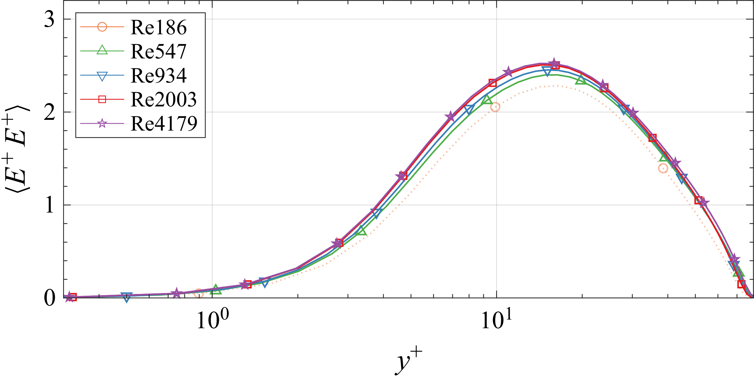


 Open access