


1. Introduction
Flow reconstruction from sparse data has received a lot of attention and the literature on the subject is vast; see for example Brunton & Noack (Reference Brunton and Noack2015), Sipp & Schmid (Reference Sipp and Schmid2016), Callaham, Maeda & Brunton (Reference Callaham, Maeda and Brunton2019), Karniadakis et al. (Reference Karniadakis, Kevrekidis, Lu, Perdikaris, Wang and Yang2021), Zaki (Reference Zaki2025) and references therein. On the other hand, forecasting the future evolution of the flow has received considerably less attention in fluid dynamics research, especially turbulence. The ability to estimate the future state from current data, also known as forecasting (Box et al. Reference Box, Jenkins, Reinsel and Ljung2015), has many applications. Examples include weather forecasting, urban safety (prediction of toxic pollutant trajectory that can guide evacuation measures), prediction of extreme events (such as heat waves) ahead of time, etc.
The forecasting time window of turbulent flows is limited by a fundamental physical constraint, which arises from the fact that such flows are chaotic and thus have extreme sensitivity to initial conditions. This is popularly known as the ’butterfly effect’ (Lorenz Reference Lorenz1963) and can be understood as follows. Consider two turbulent flows, originating from the same physical process, that have initial conditions with infinitesimally small differences. Their trajectories in phase space will diverge at a rate determined by the maximum Lyapunov exponent,
 $\lambda _1$
, that is
$\lambda _1$
, that is
 $|\delta x (t)| \sim {\rm e}^{\lambda _1 t}$
, where
$|\delta x (t)| \sim {\rm e}^{\lambda _1 t}$
, where
 $|\delta x (t)|$
is the norm of the distance between two points in phase space. The corresponding time scale is
$|\delta x (t)|$
is the norm of the distance between two points in phase space. The corresponding time scale is
 $1/\lambda _1$
.
$1/\lambda _1$
.
There are theoretical arguments (Ruelle Reference Ruelle1979; Crisanti et al. Reference Crisanti, Jensen, Vulpiani and Paladin1993; Ge, Rolland & Vassilicos Reference Ge, Rolland and Vassilicos2023) and computational evidence (Mohan, Fitzsimmons & Moser Reference Mohan, Fitzsimmons and Moser2017; Hassanaly & Raman Reference Hassanaly and Raman2019) that in turbulent flows
 $\lambda _1$
scales with the Kolmogorov time scale,
$\lambda _1$
scales with the Kolmogorov time scale,
 $\tau$
(with a correction factor that depends on Reynolds number). Therefore the future evolution of turbulent flows can only be forecast over a time window that is only several times larger than
$\tau$
(with a correction factor that depends on Reynolds number). Therefore the future evolution of turbulent flows can only be forecast over a time window that is only several times larger than
 $\tau$
, say
$\tau$
, say
 $(6{-}10) \tau$
. This has been confirmed repeatedly, irrespective of the method used for forecasting; see Pathak et al. (Reference Pathak, Lu, Hunt, Girvan and Ott2017), Vlachas et al. (Reference Vlachas, Pathak, Hunt, Sapsis, Girvan, Ott and Koumoutsakos2020), Dubois et al. (Reference Dubois, Gomez, Planckaert and Perret2020), Eivazi et al. (Reference Eivazi, Guastoni, Schlatter, Azizpour and Vinuesa2021), Khodkar & Hassanzadeh (Reference Khodkar and Hassanzadeh2021) and Constante-Amores, Linot & Graham (Reference Constante-Amores, Linot and Graham2025) for a very small sample of extensive literature on the subject. Therefore, for high-Reynolds-number flows this time window is very short to be useful in practice. For other applications, however, for example in medium-range weather forecasting, current lead times are 10 days, but can reach up to 15 days if the uncertainty in the initial conditions is reduced by an order of magnitude (Zhang et al. Reference Zhang, Sun, Magnusson, Buizza, Lin, Chen and Emanuel2019; Allen, Markou & Tebbutt Reference Allen, Markou and Tebbutt2025). This window is sufficiently large to bring about enormous socioeconomic benefits, for example protecting lives, property, etc.
$(6{-}10) \tau$
. This has been confirmed repeatedly, irrespective of the method used for forecasting; see Pathak et al. (Reference Pathak, Lu, Hunt, Girvan and Ott2017), Vlachas et al. (Reference Vlachas, Pathak, Hunt, Sapsis, Girvan, Ott and Koumoutsakos2020), Dubois et al. (Reference Dubois, Gomez, Planckaert and Perret2020), Eivazi et al. (Reference Eivazi, Guastoni, Schlatter, Azizpour and Vinuesa2021), Khodkar & Hassanzadeh (Reference Khodkar and Hassanzadeh2021) and Constante-Amores, Linot & Graham (Reference Constante-Amores, Linot and Graham2025) for a very small sample of extensive literature on the subject. Therefore, for high-Reynolds-number flows this time window is very short to be useful in practice. For other applications, however, for example in medium-range weather forecasting, current lead times are 10 days, but can reach up to 15 days if the uncertainty in the initial conditions is reduced by an order of magnitude (Zhang et al. Reference Zhang, Sun, Magnusson, Buizza, Lin, Chen and Emanuel2019; Allen, Markou & Tebbutt Reference Allen, Markou and Tebbutt2025). This window is sufficiently large to bring about enormous socioeconomic benefits, for example protecting lives, property, etc.
Is it possible to enlarge the forecasting window for turbulent flows and get estimations that are useful in engineering practice? The aforementioned scaling of
 $\lambda _1$
with
$\lambda _1$
with
 $\tau$
indicates that the former is determined by the smallest scales of the flow. However, a turbulent flow consists of a wide range of spatio-temporal structures, and it is well known that large-scale structures are slower and more organised (Pope Reference Pope2000). This opens the possibility that they can be more amenable to forecasting. These structures are important because they determine momentum transfer (and therefore forces) and scalar dispersion. The ability therefore to forecast their future evolution can bring many practical benefits. Most of existing work on forecasting to date has focused on low-dimensional dynamical systems (such the Lorenz 63/96 systems, the Kuramoto–Sivashinsky equation, the nine-equation model of Moehlis, Faisst & Eckhardt (Reference Moehlis, Faisst and Eckhardt2004)) or two-dimensional flows (such as flow in a two-dimensional lid-driven cavity). These dynamical systems, however, do not exhibit the large separation of length and time scales that is necessary to answer the question at the beginning of this paragraph. To fill this gap, the present paper considers the three-dimensional turbulent recirculating flow around a surface-mounted prism. As is seen later, this flow contains a wide range of scales, such as large organised structures and a clear inertial regime.
$\tau$
indicates that the former is determined by the smallest scales of the flow. However, a turbulent flow consists of a wide range of spatio-temporal structures, and it is well known that large-scale structures are slower and more organised (Pope Reference Pope2000). This opens the possibility that they can be more amenable to forecasting. These structures are important because they determine momentum transfer (and therefore forces) and scalar dispersion. The ability therefore to forecast their future evolution can bring many practical benefits. Most of existing work on forecasting to date has focused on low-dimensional dynamical systems (such the Lorenz 63/96 systems, the Kuramoto–Sivashinsky equation, the nine-equation model of Moehlis, Faisst & Eckhardt (Reference Moehlis, Faisst and Eckhardt2004)) or two-dimensional flows (such as flow in a two-dimensional lid-driven cavity). These dynamical systems, however, do not exhibit the large separation of length and time scales that is necessary to answer the question at the beginning of this paragraph. To fill this gap, the present paper considers the three-dimensional turbulent recirculating flow around a surface-mounted prism. As is seen later, this flow contains a wide range of scales, such as large organised structures and a clear inertial regime.
Naive application of existing dimensionality reduction methods, such as dynamic mode decomposition (DMD), for forecasting will fail. The DMD method constructs a linear model of the form
 $\boldsymbol{x}[k+1]=A \boldsymbol{x}[k]$
(see Schmid Reference Schmid2010), where
$\boldsymbol{x}[k+1]=A \boldsymbol{x}[k]$
(see Schmid Reference Schmid2010), where
 $\boldsymbol{x}[k]$
is the state vector at time instant
$\boldsymbol{x}[k]$
is the state vector at time instant
 $k$
. Recursive application of this relation results in exponentially increasing or decreasing state values, depending on whether the eigenvalues of
$k$
. Recursive application of this relation results in exponentially increasing or decreasing state values, depending on whether the eigenvalues of
 $A$
are outside or inside the unit circle, respectively. In the case of exponentially increasing values, the growth rate is not related to
$A$
are outside or inside the unit circle, respectively. In the case of exponentially increasing values, the growth rate is not related to
 $\lambda _1$
. The same problem appears for higher-order DMD, which can be put in the same linear form as the standard DMD, but now
$\lambda _1$
. The same problem appears for higher-order DMD, which can be put in the same linear form as the standard DMD, but now
 $\boldsymbol{x}[k]$
contains time-delayed variables (Le Clainche & Vega Reference Le Clainche and Vega2017).
$\boldsymbol{x}[k]$
contains time-delayed variables (Le Clainche & Vega Reference Le Clainche and Vega2017).
More advanced approaches are therefore necessary. In particular, the decomposition of chaotic dynamics into a linear model with forcing is a very attractive approach because of the availability of a large number of tools for linear systems. Recently Chu & Schmidt (Reference Chu and Schmidt2025) derived a linear, time-invariant model for the coefficients of spectral proper orthogonal decomposition (POD) modes. The authors retained the forcing term and included its dynamics in the model formulation. The presence of a stochastic forcing term results in a probabilistic representation of the future evolution of dominant structures. Brunton et al. (Reference Brunton, Brunton, Proctor, Kaiser and Kutz2017) combined time-delay embedding and Koopman theory to derive a linear model in the leading time-delay coordinates which is forced by low-energy variables. The authors call this the Hankel alternative view of Koopman (HAVOK). The underlying idea is the following. Koopman theory (Mezić Reference Mezić2013; Otto & Rowley Reference Otto and Rowley2021; Brunton et al. Reference Brunton, Budišić, Kaiser and Kutz2022) seeks a linear representation of strongly nonlinear dynamics in the space of all observables
 $\boldsymbol {y}$
, which are functions of the state
$\boldsymbol {y}$
, which are functions of the state
 $\boldsymbol {x}$
of the system, i.e.
$\boldsymbol {x}$
of the system, i.e.
 $\boldsymbol {y}=\boldsymbol {g}(\boldsymbol {x})$
. It therefore trades the finite dimensionality of the nonlinear system to the infinite dimensional dynamics of the linear system. In DMD,
$\boldsymbol {y}=\boldsymbol {g}(\boldsymbol {x})$
. It therefore trades the finite dimensionality of the nonlinear system to the infinite dimensional dynamics of the linear system. In DMD,
 $\boldsymbol {y}=\boldsymbol {x}$
, but this selection of observables may not be rich enough for many nonlinear systems. The main idea of HAVOK is to construct a forced linear model using as states not
$\boldsymbol {y}=\boldsymbol {x}$
, but this selection of observables may not be rich enough for many nonlinear systems. The main idea of HAVOK is to construct a forced linear model using as states not
 $\boldsymbol {x}$
, but instead time-delayed coordinates that contain more information about the system. This is in accordance with the Takens (Reference Takens1981) embedding theorem; the theorem allows the construction of an attractor from a time series of a single measurement that is diffeomorphic to the original chaotic attractor (diffeomorphic means that a smooth, invertible transformation exists between the original attractor and its representation). A linear model cannot capture multiple fixed points, so the model is forced by an (unclosed) term. The model states are obtained from the right singular vectors of the Hankel matrix which is assembled by stacking time-delayed values of observables column by column, and each column is advanced one time unit ahead of the previous column. It is found that the forcing is active only in the regions of the chaotic attractor with strong nonlinearity (e.g. when switching between the two lobes in the Lorenz attractor), and its statistics are non-Gaussian. In Khodkar & Hassanzadeh (Reference Khodkar and Hassanzadeh2021) the forcing is found from vector-valued observables in a physics-informed way or a purely data-driven fashion, depending on whether any knowledge of governing dynamics was available or not. In Dylewsky et al. (Reference Dylewsky, Kaiser, Brunton and Kutz2022) the forcing is obtained in a two-step process in a fully unsupervised manner.
$\boldsymbol {x}$
, but instead time-delayed coordinates that contain more information about the system. This is in accordance with the Takens (Reference Takens1981) embedding theorem; the theorem allows the construction of an attractor from a time series of a single measurement that is diffeomorphic to the original chaotic attractor (diffeomorphic means that a smooth, invertible transformation exists between the original attractor and its representation). A linear model cannot capture multiple fixed points, so the model is forced by an (unclosed) term. The model states are obtained from the right singular vectors of the Hankel matrix which is assembled by stacking time-delayed values of observables column by column, and each column is advanced one time unit ahead of the previous column. It is found that the forcing is active only in the regions of the chaotic attractor with strong nonlinearity (e.g. when switching between the two lobes in the Lorenz attractor), and its statistics are non-Gaussian. In Khodkar & Hassanzadeh (Reference Khodkar and Hassanzadeh2021) the forcing is found from vector-valued observables in a physics-informed way or a purely data-driven fashion, depending on whether any knowledge of governing dynamics was available or not. In Dylewsky et al. (Reference Dylewsky, Kaiser, Brunton and Kutz2022) the forcing is obtained in a two-step process in a fully unsupervised manner.
The combination of Koopman theory with time-delayed embeddings has opened new directions for the representation of a chaotic system as a forced linear model and has spawned important theoretical work (Kamb et al. Reference Kamb, Kaiser, Brunton and Kutz2020; Arbabi & Mezić Reference Arbabi and Mezić2017; Pan & Duraisamy Reference Pan and Duraisamy2019, Reference Pan and Duraisamy2020; Giannakis Reference Giannakis2019; Das & Giannakis Reference Das and Giannakis2019). The connection between the left-singular vectors of the time-delayed Hankel matrix and the space–time POD, space-only POD and spectral POD modes was established in Frame & Towne (Reference Frame and Towne2023).
The contribution of the present paper is to add one more piece to the aforementioned time-delayed embedding/Koopman framework. More specifically, we combine this framework with linear optimal estimation theory (Kailath, Hassibi & Sayed Reference Kailath, Hassibi and Sayed2000) that allows us to derive a mapping from sparse measurements at the current time instant to the velocity field at future time instants. This approach is useful because it provides an estimate of the forcing term and thereby closes the system. Schmidt (Reference Schmidt2026) proposed a method that does not require a forcing term. This was achieved by leveraging the correlation between hindcast and forecast datasets with the aid of extended POD. To forecast the future evolution of the flow, data are required for the full flow, while in our method, once the mapping has been established, only data from a few sensors are required. A nonlinear mapping that employs machine learning techniques (instead of Koopman theory) was proposed recently for weather forecasting by Allen et al. (Reference Allen, Markou and Tebbutt2025).
Our approach is applied to flow around a surface-mounted cube, as already mentioned. Scalar is released from a source placed upstream of the cube. We derive the mapping from current to future states using not only velocity data but also scalar data; scalar sensors are usually cheaper to acquire. The proposed estimator is scalable, physically interpretable and provides sequential forecasting on a rolling time window as streaming data are coming in. Of particular interest is the quality of forecasting and how it varies with the size of the time window.
The paper is structured as follows. Sections 2 and 3 describe the forecasting methodology from sparse velocity and scalar data, respectively. Results are presented and discussed in § 4. Section 5 summarises the main findings of the paper and outlines some future research directions.
2. Flow forecasting from sparse velocity measurements
In the following,
 $u,v,w$
(interchangeably used with
$u,v,w$
(interchangeably used with
 $u_1,u_2,u_3$
) are the three velocity components in the Cartesian directions
$u_1,u_2,u_3$
) are the three velocity components in the Cartesian directions
 $x,y,z$
, respectively. Time averages are designated with angular brackets and fluctuations with a prime; for example
$x,y,z$
, respectively. Time averages are designated with angular brackets and fluctuations with a prime; for example
 $\langle u \rangle$
and
$\langle u \rangle$
and
 $u^\prime$
are the mean and fluctuating velocities, respectively, in the
$u^\prime$
are the mean and fluctuating velocities, respectively, in the
 $x$
direction.
$x$
direction.
We first describe how to forecast the future evolution of a turbulent flow from a set of sparse velocity measurements that record current information. In the following section, we extend the idea to sparse scalar measurements.
The method comprises three steps.
2.1. Step 1: dimensionality reduction
To make the method applicable to three-dimensional turbulent flows, we first need to reduce the number of degrees of freedom. In this paper we use POD (Sirovich Reference Sirovich1987). This method provides a linear mapping between the velocity field and the POD coefficients; we exploit this linearity later in step 3.
To get the POD modes, the snapshot matrix
 $\boldsymbol{Y}(\boldsymbol{x},t_{1}:t_{K})$
for the velocity fluctuations
$\boldsymbol{Y}(\boldsymbol{x},t_{1}:t_{K})$
for the velocity fluctuations
 $u^{\prime }$
,
$u^{\prime }$
,
 $v^{\prime }$
and
$v^{\prime }$
and
 $w^{\prime }$
is assembled:
$w^{\prime }$
is assembled:
 \begin{equation} \boldsymbol{Y}(\boldsymbol{x},t_{1}:t_{K}) = \left [ \begin{array}{cccc} u^{\prime }(\boldsymbol{x}_{1}, t_{1})& u^{\prime }(\boldsymbol{x}_{1}, t_{2})& \ldots & u^{\prime }(\boldsymbol{x}_{1}, t_{K})\\ \vdots & \vdots & \ldots & \vdots \\ u^{\prime }(\boldsymbol{x}_{N}, t_{1})& u^{\prime }(\boldsymbol{x}_{N}, t_{2})& \ldots & u^{\prime }(\boldsymbol{x}_{N}, t_{K})\\ v^{\prime }(\boldsymbol{x}_{1}, t_{1})& v^{\prime }(\boldsymbol{x}_{1}, t_{2})& \ldots & v^{\prime }(\boldsymbol{x}_{1}, t_{K})\\ \vdots & \vdots & \ldots & \vdots \\ v^{\prime }(\boldsymbol{x}_{N}, t_{1})& v^{\prime }(\boldsymbol{x}_{N}, t_{2})& \ldots & v^{\prime }(\boldsymbol{x}_{N, t_{K}})\\ w^{\prime }(\boldsymbol{x}_{1}, t_{1})& w^{\prime }(\boldsymbol{x}_{1}, t_{2})& \ldots & w^{\prime }(\boldsymbol{x}_{1}, t_{K})\\ \vdots & \vdots & \ldots & \vdots \\ w^{\prime }(\boldsymbol{x}_{N}, t_{1})& w^{\prime }(\boldsymbol{x}_{N}, t_{2})& \ldots & w^{\prime }(\boldsymbol{x}_{N, t_{K}}) \end{array} \right ] , \end{equation}
where
 $\boldsymbol{Y} \in \mathbb{R}^{3N \times K}$
,
$\boldsymbol{Y} \in \mathbb{R}^{3N \times K}$
,
 $\boldsymbol{x}_{i}= [x_{i}, y_{i}, z_{i} ]\ (i=1,2,\ldots ,N)$
is the location vector for the
$\boldsymbol{x}_{i}= [x_{i}, y_{i}, z_{i} ]\ (i=1,2,\ldots ,N)$
is the location vector for the
 $i$
th spatial location,
$i$
th spatial location,
 $N$
is the number of cells and
$N$
is the number of cells and
 $K$
is the total number of snapshots. The spacing between successive snapshots is
$K$
is the total number of snapshots. The spacing between successive snapshots is
 $\Delta t$
. Singular value decomposition (SVD) is performed on the weighted matrix
$\Delta t$
. Singular value decomposition (SVD) is performed on the weighted matrix
 $\mathcal{V}^{1/2} \boldsymbol{Y}$
:
$\mathcal{V}^{1/2} \boldsymbol{Y}$
:
 \begin{equation} \mathcal{V}^{1/2} \boldsymbol{Y}= \boldsymbol{U}_{\!Y} \boldsymbol{ \mathit{\varSigma } }_{Y} \boldsymbol{V}^{\top }_{Y}, \end{equation}
where
 $\mathcal{V}=diag (V_1, V_2 \ldots V_N, V_1, V_2, \ldots , V_N, V_1, V_2, \ldots , V_N )$
is a diagonal matrix with the cell volumes
$\mathcal{V}=diag (V_1, V_2 \ldots V_N, V_1, V_2, \ldots , V_N, V_1, V_2, \ldots , V_N )$
is a diagonal matrix with the cell volumes
 $V_i$
in the main diagonal,
$V_i$
in the main diagonal,
 $\boldsymbol{U}_{\!Y} \in \mathbb{R}^{3N \times K}$
contains the left singular vectors,
$\boldsymbol{U}_{\!Y} \in \mathbb{R}^{3N \times K}$
contains the left singular vectors,
 $\boldsymbol{ \mathit{\varSigma } }_{Y} \in \mathbb{R}^{K \times K}$
is a diagonal matrix that stores
$\boldsymbol{ \mathit{\varSigma } }_{Y} \in \mathbb{R}^{K \times K}$
is a diagonal matrix that stores
 $K$
singular values (we assume
$K$
singular values (we assume
 $K \ll 3N$
) and
$K \ll 3N$
) and
 $\boldsymbol{V}_{Y} \in \mathbb{R}^{K \times K}$
contains the right singular vectors. The scaled POD eigenmodes
$\boldsymbol{V}_{Y} \in \mathbb{R}^{K \times K}$
contains the right singular vectors. The scaled POD eigenmodes
 $U_{Y, k}(\boldsymbol{x})$
are extracted from the columns of
$U_{Y, k}(\boldsymbol{x})$
are extracted from the columns of
 $\boldsymbol{U}_{\!Y}$
from
$\boldsymbol{U}_{\!Y}$
from
 \begin{equation} {U}_{Y} (\boldsymbol{x}) = \mathcal{V}^{-1/2} \boldsymbol{U}_{\!Y}. \end{equation}
The singular values
 $\sigma _{Y, k}$
are ranked in descending order along the diagonal of matrix
$\sigma _{Y, k}$
are ranked in descending order along the diagonal of matrix
 $\boldsymbol{ \mathit{\varSigma } }_{Y}$
. The energy content of each mode is computed using
$\boldsymbol{ \mathit{\varSigma } }_{Y}$
. The energy content of each mode is computed using
 \begin{equation} \lambda _{Y, k}=\frac { \sigma ^{2}_{Y, k} }{K} \quad (k=1\ldots K) \end{equation}
and the time coefficients from
 \begin{equation} \boldsymbol{a} (t)= \boldsymbol{ \mathit{Y} }^{\top } \mathcal{V}^{1/2} \boldsymbol{U}_{\!Y}. \end{equation}
The fluctuating velocity field can be written as
 \begin{equation} u^{\prime }_{i}(x,y,z,t) = \sum ^{ K }_{k=1} a_{k}(t) {U}^{(i)}_{Y, k}(x,y,z) \approx \sum ^{m_{u}}_{k=1} a_{k}(t) {U}^{(i)}_{Y, k}(x,y,z) \quad (i=1, 2, 3), \end{equation}
where
 $m_{u}$
is the number of retained POD modes,
$m_{u}$
is the number of retained POD modes,
 $a_{k}(t)$
is the time coefficient of the
$a_{k}(t)$
is the time coefficient of the
 $k$
th POD mode and
$k$
th POD mode and
 ${U}^{(i)}_{Y, k}$
is the
${U}^{(i)}_{Y, k}$
is the
 $k$
th POD eigenvector of the
$k$
th POD eigenvector of the
 $i$
th velocity component. This expression can be written in matrix form as
$i$
th velocity component. This expression can be written in matrix form as
 \begin{equation} \underbrace {\left [ \begin{array}{c} u_1^{\prime } \\[5pt] u_2^{\prime }\\[5pt] u_3^{\prime }\end{array} \right ]} _{\equiv \boldsymbol{u}^{\prime }} = \underbrace {\left [ \begin{array}{cccc} {U}^{(1)}_{Y, 1} & {U}^{(1)}_{Y, 2} & \ldots & {U}^{(1)}_{Y, m_u} \\[5pt] {U}^{(2)}_{Y, 1} & {U}^{(2)}_{Y, 2} & \ldots & {U}^{(2)}_{Y, m_u} \\[5pt] {U}^{(3)}_{Y, 1} & {U}^{(3)}_{Y, 2} & \ldots & {U}^{(3)}_{Y, m_u} \end{array} \right ]}_{\equiv \boldsymbol{U}_{\!Y}} \underbrace {\left [ \begin{array}{c} a_1^{\prime } \\[5pt] a_2^{\prime }\\[5pt] \vdots \\[5pt] a_{m_u}^{\prime }\end{array} \right ]}_{\equiv \boldsymbol{a}} \end{equation}
or more compactly
 \begin{equation} \boldsymbol{u}^{\prime }(x,y,z,t)=\boldsymbol{U}_{\!Y}(x,y,z) \boldsymbol{a}(t). \end{equation}
2.2. Step 2: construction of a dynamical system for current and future POD coefficients
The next step is the construction of a model for the dynamic evolution of POD coefficients. This model should be able to forecast the future time signal from current information. To this end, we assemble the time-delayed Hankel matrix
 $\boldsymbol{H}$
that consists of the POD coefficients of the retained
$\boldsymbol{H}$
that consists of the POD coefficients of the retained
 $m_{u}$
velocity modes:
$m_{u}$
velocity modes:
 \begin{equation} \boldsymbol{H} = \left [ \begin{array}{cccc} \boldsymbol{a}(t_{1})& \boldsymbol{a}(t_{2})& \ldots & \boldsymbol{a}(t_{p})\\ \boldsymbol{a}(t_{2})& \boldsymbol{a}(t_{3})& \ldots & \boldsymbol{a}(t_{p+1})\\ \vdots & \vdots & \ddots & \vdots \\ \boldsymbol{a}(t_{q})& \boldsymbol{a}(t_{q+1})& \ldots & \boldsymbol{a}(t_{K_{\textit{train}}}) \end{array} \right ] , \end{equation}
where
 $ \boldsymbol{a}(t_{j})= [a_1(t_j)\ldots a_{m_u}(t_j) ]^\top$
and we use
$ \boldsymbol{a}(t_{j})= [a_1(t_j)\ldots a_{m_u}(t_j) ]^\top$
and we use
 $q$
vectors in each column. The number of columns is
$q$
vectors in each column. The number of columns is
 $p=K_{\textit{train}}-q+1$
, where
$p=K_{\textit{train}}-q+1$
, where
 $K_{\textit{train}}$
is the number of snapshots for the training dataset and
$K_{\textit{train}}$
is the number of snapshots for the training dataset and
 $\boldsymbol{H} \in \mathbb{R}^{ ( m_{u} \times q ) \times p}$
. Performing SVD on
$\boldsymbol{H} \in \mathbb{R}^{ ( m_{u} \times q ) \times p}$
. Performing SVD on
 $\boldsymbol{H}$
, we obtain
$\boldsymbol{H}$
, we obtain
 \begin{equation} \boldsymbol{H} \approx \boldsymbol{U}_{\!H} \boldsymbol{\varSigma }_{H} \boldsymbol{V}^{\top }_{H}, \end{equation}
where
 $\boldsymbol{U}_{\!H} \in \mathbb{R}^{ ( m_{u} \times q ) \times r}$
,
$\boldsymbol{U}_{\!H} \in \mathbb{R}^{ ( m_{u} \times q ) \times r}$
,
 $\boldsymbol{\varSigma }_{H} \in \mathbb{R}^{r \times r}$
,
$\boldsymbol{\varSigma }_{H} \in \mathbb{R}^{r \times r}$
,
 $\boldsymbol{V}_{H} \in \mathbb{R}^{p \times r}$
and
$\boldsymbol{V}_{H} \in \mathbb{R}^{p \times r}$
and
 $r$
is the number of retained singular values. The matrix of the left singular vectors
$r$
is the number of retained singular values. The matrix of the left singular vectors
 $\boldsymbol{U}_{\!H}$
can be explicitly written as
$\boldsymbol{U}_{\!H}$
can be explicitly written as
 \begin{equation} \boldsymbol{U}_{\!H} = \left [ \begin{array}{cccc} \boldsymbol{U}^{(u,v,w)}_{H, 1}(t_{1})& \boldsymbol{U}^{(u,v,w)}_{H, 2}(t_{1})& \ldots & \boldsymbol{U}^{(u,v,w)}_{H, r}(t_{1})\\[5pt] \boldsymbol{U}^{(u,v,w)}_{H, 1}(t_{2})& \boldsymbol{U}^{(u,v,w)}_{H, 2}(t_{2})& \ldots & \boldsymbol{U}^{(u,v,w)}_{H, r}(t_{2})\\[5pt] \vdots & \vdots & \ddots & \vdots \\[5pt] \boldsymbol{U}^{(u,v,w)}_{H, 1}(t_{q})& \boldsymbol{U}^{(u,v,w)}_{H, 2}(t_{q})& \ldots & \boldsymbol{U}^{(u,v,w)}_{H, r}(t_{q}) \end{array} \right ] , \end{equation}
where each column
 $\boldsymbol{U}^{(u,v,w)}_{H,i}(t_{1} \colon t_{q}) \in \mathbb{R}^{m_{u} \times q }$
is the
$\boldsymbol{U}^{(u,v,w)}_{H,i}(t_{1} \colon t_{q}) \in \mathbb{R}^{m_{u} \times q }$
is the
 $i$
th time-delayed singular mode of the Hankel matrix.
$i$
th time-delayed singular mode of the Hankel matrix.
The diagonal matrix of singular values
 $\boldsymbol{\varSigma }_{H}$
is
$\boldsymbol{\varSigma }_{H}$
is
 \begin{equation} \boldsymbol{\varSigma }_{H} = \left [ \begin{array}{cccc} \sigma _{H, 1}& 0& \ldots & 0\\ 0& \sigma _{H, 2}& \ldots & 0\\ \vdots & \vdots & \ddots & \vdots \\ 0& 0& \ldots & \sigma _{H, r} \end{array} \right ] , \end{equation}
and the matrix of the right singular vectors
 $\boldsymbol{V}_{H}$
can be explicitly written as
$\boldsymbol{V}_{H}$
can be explicitly written as
 \begin{equation} \boldsymbol{V}_{H} = \left [ \begin{array}{cccc} v_{H,1}(t_{1})& v_{H,1}(t_{2})& \ldots & v_{H,1}(t_{p})\\[3pt] v_{H,2}(t_{1})& v_{H,2}(t_{2})& \ldots & v_{H,2}(t_{p})\\ \vdots & \vdots & \ddots & \vdots \\ v_{H,r}(t_{1})& v_{H,r}(t_{2})& \ldots & v_{H,r}(t_{p}) \end{array} \right ] . \end{equation}
We now define the vector
 $\boldsymbol{v}_{H}(t_j)=[v_{H, 1}(t_j), v_{H, 2}(t_j), \ldots , v_{H, r}(t_j)]^{\top } \in \mathbb{R}^{r}$
 $(j=1 \ldots p)$
extracted from the columns of matrix
$(j=1 \ldots p)$
extracted from the columns of matrix
 $\boldsymbol{V}_{H}$
. We consider
$\boldsymbol{V}_{H}$
. We consider
 $\boldsymbol{v}_{H}$
as the state variable of the following discrete-in-time, forced, linear dynamical system:
$\boldsymbol{v}_{H}$
as the state variable of the following discrete-in-time, forced, linear dynamical system:
 \begin{equation} \boldsymbol{v}_{H}[k+1] = \boldsymbol{A} \boldsymbol{v}_{H}[k]+ \boldsymbol{w}_{2}[k], \end{equation}
where
 $\boldsymbol{v}_{H}[k]=\boldsymbol{v}_{H}[t_k]$
,
$\boldsymbol{v}_{H}[k]=\boldsymbol{v}_{H}[t_k]$
,
 $k=1 \ldots p-1$
and
$k=1 \ldots p-1$
and
 $\boldsymbol{A} \in \mathbb{R}^{r \times r}$
.
$\boldsymbol{A} \in \mathbb{R}^{r \times r}$
.
To obtain matrix
 $\boldsymbol{A}$
, we write (2.14) explicitly for
$\boldsymbol{A}$
, we write (2.14) explicitly for
 $k=1 \ldots p-1$
:
$k=1 \ldots p-1$
:
 \begin{align} \boldsymbol{v}_{H}[2] & \approx \boldsymbol{A}\boldsymbol{v}_{H}[1], \end{align}
 \begin{align} \boldsymbol{v}_{H}[3] & \approx \boldsymbol{A}\boldsymbol{v}_{H}[2],\nonumber \\ & \vdots \end{align}
 \begin{align} \boldsymbol{v}_{H}[p] & \approx \boldsymbol{A}\boldsymbol{v}_{H}[p-1]. \end{align}
In matrix form, this becomes
 \begin{equation} \boldsymbol{V}^{\prime } \approx \boldsymbol{A} \boldsymbol{V}, \end{equation}
where
 $\boldsymbol{V}^{\prime }, \boldsymbol{V} \in \mathbb{R}^{r \times (p-1)}$
:
$\boldsymbol{V}^{\prime }, \boldsymbol{V} \in \mathbb{R}^{r \times (p-1)}$
:
 \begin{align} \boldsymbol{V}^{\prime } & = \left [ \begin{array}{cccc} \boldsymbol{v}_{H}[2]& \boldsymbol{v}_{H}[3]& \ldots & \boldsymbol{v}_{H}[p] \end{array} \right ]^{\top }, \end{align}
 \begin{align} \boldsymbol{V} & = \left [ \begin{array}{cccc} \boldsymbol{v}_{H}[1]& \boldsymbol{v}_{H}[2]& \ldots & \boldsymbol{v}_{H}[p-1] \end{array} \right ]^{\top }. \end{align}
Then the system matrix
 $\boldsymbol{A}$
can be calculated from
$\boldsymbol{A}$
can be calculated from
 \begin{equation} \boldsymbol{V}^{\prime } = \boldsymbol{A} {\boldsymbol{V}} \Rightarrow \boldsymbol{V}^{\prime } {\boldsymbol{V}}^{\top } = \boldsymbol{A} {\boldsymbol{V}} {\boldsymbol{V}}^{\top } \Rightarrow \boldsymbol{A} = \boldsymbol{V}^{\prime } {\boldsymbol{V}}^{\top } \big ( {\boldsymbol{V}} {\boldsymbol{V}}^{\top } \big )^{-1}. \end{equation}
This formulation essentially applies the DMD algorithm directly to
 $ \boldsymbol{v}_{H}[k]$
.
$ \boldsymbol{v}_{H}[k]$
.
Once
 $\boldsymbol{A}$
is known, the forcing
$\boldsymbol{A}$
is known, the forcing
 $\boldsymbol{w}_{2}[k]$
can be easily computed from the training dataset,
$\boldsymbol{w}_{2}[k]$
can be easily computed from the training dataset,
 $\boldsymbol{w}_{2}[k]=\boldsymbol{v}_{H}[k+1]-\boldsymbol{A} \boldsymbol{v}_{H}[k]$
. The covariance matrix of the forcing
$\boldsymbol{w}_{2}[k]=\boldsymbol{v}_{H}[k+1]-\boldsymbol{A} \boldsymbol{v}_{H}[k]$
. The covariance matrix of the forcing
 $\boldsymbol{Q} \in \mathbb{R}^{r \times r}$
can be obtained from
$\boldsymbol{Q} \in \mathbb{R}^{r \times r}$
can be obtained from
 \begin{equation} \boldsymbol{Q} = \mathbb{E} \big ( \boldsymbol{w}_{2}\boldsymbol{w}^{\top }_{2} \big ) = \frac {1}{p-1} \sum ^{k=p-1}_{k=1} \boldsymbol{w}_{2}[k] \boldsymbol{w}^{\top }_{2}[k]. \end{equation}
It is important to notice that using
 $\boldsymbol{v}_{H}[k]$
we can obtain the current (at instant
$\boldsymbol{v}_{H}[k]$
we can obtain the current (at instant
 $k$
) and forecast the future (at instants
$k$
) and forecast the future (at instants
 $k+1 \ldots k+q$
) time coefficients as follows:
$k+1 \ldots k+q$
) time coefficients as follows:
 \begin{eqnarray} \left [ \begin{array}{c} \boldsymbol{a}[k] \\[3pt] \boldsymbol{a}[k+1] \\ \vdots \\ \boldsymbol{a} [k+q] \\ \end{array} \right ] & = & \boldsymbol{U}_{\!H} \varSigma _{H} \boldsymbol{v}_{H}[k]. \end{eqnarray}
In particular
 $\boldsymbol{a}[k]$
can be obtained from
$\boldsymbol{a}[k]$
can be obtained from
 \begin{equation} \boldsymbol{a}[k] = \underbrace {\boldsymbol{U}_{\!H}(t_{1}) \varSigma _{H}} _{\equiv \boldsymbol{C}} \boldsymbol{v}_{H}[k] ,\end{equation}
where
 $\boldsymbol{C} \in \mathbb{R}^{m_{u} \times r}$
and
$\boldsymbol{C} \in \mathbb{R}^{m_{u} \times r}$
and
 $\boldsymbol{U}_{\!H}(t_{1})= [ \begin{array}{cccc} \boldsymbol{U}^{(u,v,w)}_{H, 1}(t_{1})& \boldsymbol{U}^{(u,v,w)}_{H, 2}(t_{1})& \ldots & \boldsymbol{U}^{(u,v,w)}_{H, r}(t_{1}) \end{array} ] \in \mathbb{R}^{m_{u} \times r}$
is the top row of matrix
$\boldsymbol{U}_{\!H}(t_{1})= [ \begin{array}{cccc} \boldsymbol{U}^{(u,v,w)}_{H, 1}(t_{1})& \boldsymbol{U}^{(u,v,w)}_{H, 2}(t_{1})& \ldots & \boldsymbol{U}^{(u,v,w)}_{H, r}(t_{1}) \end{array} ] \in \mathbb{R}^{m_{u} \times r}$
is the top row of matrix
 $\boldsymbol{U}_{\!H}$
; see (2.11).
$\boldsymbol{U}_{\!H}$
; see (2.11).
The previous two expressions demonstrate the fundamental importance of
 $\boldsymbol{U}_{\!H}$
. This matrix has a very clear physical interpretation, which can be understood as follows. Each column of
$\boldsymbol{U}_{\!H}$
. This matrix has a very clear physical interpretation, which can be understood as follows. Each column of
 $\boldsymbol{H}$
contains
$\boldsymbol{H}$
contains
 $q$
snapshots, i.e. short time-varying sequences of fixed time duration (instead of a single snapshot as in standard POD). There are
$q$
snapshots, i.e. short time-varying sequences of fixed time duration (instead of a single snapshot as in standard POD). There are
 $p$
such short sequences in total. The left singular vectors
$p$
such short sequences in total. The left singular vectors
 $\boldsymbol{U}^{(u,v,w)}_{H,i}$
are obtained by performing SVD on
$\boldsymbol{U}^{(u,v,w)}_{H,i}$
are obtained by performing SVD on
 $\boldsymbol{H}$
. These vectors capture the most important time-dependent patterns, in exactly the same way as the POD modes capture the most important (static) patterns from a series of snapshots. These time-varying patterns are arranged column by column in descending order of importance, as quantified by the singular values
$\boldsymbol{H}$
. These vectors capture the most important time-dependent patterns, in exactly the same way as the POD modes capture the most important (static) patterns from a series of snapshots. These time-varying patterns are arranged column by column in descending order of importance, as quantified by the singular values
 $\sigma _{H,k}$
, and can be exploited to predict the future evolution from current information. They resemble Legendre polynomials for short
$\sigma _{H,k}$
, and can be exploited to predict the future evolution from current information. They resemble Legendre polynomials for short
 $q \times \Delta t$
and become sinusoids for large
$q \times \Delta t$
and become sinusoids for large
 $q \times \Delta t$
(see Dylewsky et al. Reference Dylewsky, Kaiser, Brunton and Kutz2022; Frame & Towne Reference Frame and Towne2023). We visualise these patterns for the flow around a surface-mounted cube in §§ 4.4 and 4.5.
$q \times \Delta t$
(see Dylewsky et al. Reference Dylewsky, Kaiser, Brunton and Kutz2022; Frame & Towne Reference Frame and Towne2023). We visualise these patterns for the flow around a surface-mounted cube in §§ 4.4 and 4.5.
Note that this step is independent of the dimensionality reduction method selected in step 1. The question now is how to obtain
 $\boldsymbol{v}_{H}[k]$
since the forcing term
$\boldsymbol{v}_{H}[k]$
since the forcing term
 $\boldsymbol{w}_{2}[k]$
in (2.14) is not known. We can get a closure if measurements at some sparse sensor points are available.
$\boldsymbol{w}_{2}[k]$
in (2.14) is not known. We can get a closure if measurements at some sparse sensor points are available.
2.3. Step 3: closure of the system using sensor measurements
Let us assume that we have a set of
 $l$
velocity measurements
$l$
velocity measurements
 $\boldsymbol{s}[k] \in \mathbb{R}^{l}$
at a number of sensor points. At each sensor, one or more velocity components are recorded. We can express
$\boldsymbol{s}[k] \in \mathbb{R}^{l}$
at a number of sensor points. At each sensor, one or more velocity components are recorded. We can express
 $\boldsymbol{s}[k]$
in terms of
$\boldsymbol{s}[k]$
in terms of
 $\boldsymbol{a}[k]$
as follows:
$\boldsymbol{a}[k]$
as follows:
 \begin{equation} \boldsymbol{s}[k] = \boldsymbol{S} \boldsymbol{U}_{\!Y} \boldsymbol{a}[k] + \boldsymbol{g}[k], \end{equation}
where matrix
 $\boldsymbol{S}$
selects the rows of the POD mode matrix
$\boldsymbol{S}$
selects the rows of the POD mode matrix
 $\boldsymbol{U}_{\!Y}$
corresponding to the sensor location and the velocity component being measured (it is
$\boldsymbol{U}_{\!Y}$
corresponding to the sensor location and the velocity component being measured (it is
 $0$
everywhere except for those points and components where the corresponding element is equal to
$0$
everywhere except for those points and components where the corresponding element is equal to
 $1$
). Vector
$1$
). Vector
 $\boldsymbol{g} \in \mathbb{R}^{l}$
includes measurement errors as well as errors due to POD mode truncation (because only
$\boldsymbol{g} \in \mathbb{R}^{l}$
includes measurement errors as well as errors due to POD mode truncation (because only
 $m_u$
modes are retained). The elements of
$m_u$
modes are retained). The elements of
 $\boldsymbol{g}[k]$
can be obtained from the training dataset,
$\boldsymbol{g}[k]$
can be obtained from the training dataset,
 $\boldsymbol{g}[k]=\boldsymbol{s}[k]-\boldsymbol{S} \boldsymbol{U}_{\!Y} \boldsymbol{a}[k]$
), and its covariance
$\boldsymbol{g}[k]=\boldsymbol{s}[k]-\boldsymbol{S} \boldsymbol{U}_{\!Y} \boldsymbol{a}[k]$
), and its covariance
 $\boldsymbol{R} \in \mathbb{R}^{l \times l}$
can be easily calculated from
$\boldsymbol{R} \in \mathbb{R}^{l \times l}$
can be easily calculated from
 \begin{equation} \boldsymbol{R} = \mathbb{E} \big ( \boldsymbol{g}\boldsymbol{g}^{\top } \big ) = \frac {1}{p-1} \sum ^{k=p-1}_{k=1} \boldsymbol{g}[k] \boldsymbol{g}^{\top }[k]. \end{equation}
We are now ready to design a Kalman filter to estimate
 $\boldsymbol{v}_{H}[k]$
from the sparse measurements
$\boldsymbol{v}_{H}[k]$
from the sparse measurements
 $\boldsymbol{s}[k]$
. The filter takes the form
$\boldsymbol{s}[k]$
. The filter takes the form
 \begin{align} \hat {\boldsymbol{v}}_{H}[k+1] & = \boldsymbol{A} \hat {\boldsymbol{v}}_{H}[k] + \mathcal{L} \big ( \boldsymbol{s}[k]-\hat {\boldsymbol{s}}[k] \big ), \end{align}
 \begin{align} \hat {\boldsymbol{a}}[k] & = \boldsymbol{C} \hat {\boldsymbol{v}}_{H}[k], \end{align}
 \begin{align} \hat {\boldsymbol{s}}[k] & = \boldsymbol{S} \boldsymbol{U}_{\!Y} \hat {\boldsymbol{a}}[k] = \boldsymbol{S} \boldsymbol{U}_{\!Y} \boldsymbol{C} \hat {\boldsymbol{v}}_{H}[k], \end{align}
where a hat
 $\hat {()}$
denotes an estimated quantity and
$\hat {()}$
denotes an estimated quantity and
 $\mathcal{L} \in \mathbb{R}^{r \times l}$
is the Kalman filter gain. The latter is obtained from the solution of the following Riccati equation:
$\mathcal{L} \in \mathbb{R}^{r \times l}$
is the Kalman filter gain. The latter is obtained from the solution of the following Riccati equation:
 \begin{align} \boldsymbol{P} & = \boldsymbol{A}\kern-1pt\boldsymbol{P}\!\boldsymbol{A}^{T} - \boldsymbol{A}\kern-1pt\boldsymbol{P} (\boldsymbol{S} \boldsymbol{U}_{\!Y} \boldsymbol{C})^{T} ( \boldsymbol{S} \boldsymbol{U}_{\!Y} \boldsymbol{C}\kern-1pt\boldsymbol{P} (\boldsymbol{S} \boldsymbol{U}_{\!Y} \boldsymbol{C})^{T} + \boldsymbol{R} )^{-1} \boldsymbol{S} \boldsymbol{U}_{\!Y} \boldsymbol{C}\kern-1pt\boldsymbol{P}\!\boldsymbol{A}^{T} + \boldsymbol{Q}, \end{align}
 \begin{align} \mathcal{L} & = \boldsymbol{A}\kern-1pt\boldsymbol{P} (\boldsymbol{S} \boldsymbol{U}_{\!Y} \boldsymbol{C})^{T} ( \boldsymbol{S} \boldsymbol{U}_{\!Y} \boldsymbol{C}\kern-1pt\boldsymbol{P} (\boldsymbol{S} \boldsymbol{U}_{\!Y} \boldsymbol{C})^{T} + \boldsymbol{R} )^{-1}. \end{align}
From
 $\hat {\boldsymbol{v}}_{H}[k]$
one can estimate the current and future POD coefficients from (2.20), and of course the instantaneous velocity field from (2.8).
$\hat {\boldsymbol{v}}_{H}[k]$
one can estimate the current and future POD coefficients from (2.20), and of course the instantaneous velocity field from (2.8).
The linear mapping between the velocity and POD coefficients, (2.22), has allowed us to synthesise a Kalman filter. This type of filter is suitable only for linear dynamical systems and linear mappings between the measurement and state variables. For nonlinear mappings, one can use an extended Kalman filter or an ensemble Kalman filter (Evensen Reference Evensen2003). Note also that the formulation can accommodate data from moving sensor locations (e.g. data from drones); this is achieved by using a time-dependent selection matrix
 $\boldsymbol{S}[k]$
in (2.22). In this case, the filter gain
$\boldsymbol{S}[k]$
in (2.22). In this case, the filter gain
 $\mathcal{L}[k]$
will be also time-dependent. A machine learning technique (instead of Koopman/Kalman filter theory) was proposed recently by Allen et al. (Reference Allen, Markou and Tebbutt2025); it maps measurements
$\mathcal{L}[k]$
will be also time-dependent. A machine learning technique (instead of Koopman/Kalman filter theory) was proposed recently by Allen et al. (Reference Allen, Markou and Tebbutt2025); it maps measurements
 $\boldsymbol{s}[k]$
directly to the future states for weather forecasting.
$\boldsymbol{s}[k]$
directly to the future states for weather forecasting.
Steps 1 and 2 are performed offline using a training dataset. The Kalman estimator in step 3 runs online and requires only the streaming measurement data
 $\boldsymbol{s}[k]$
. The arriving data are then mapped to the future velocity field on a rolling time window through (2.24), then (2.20) and finally (2.8). Depending on the number of retained modes
$\boldsymbol{s}[k]$
. The arriving data are then mapped to the future velocity field on a rolling time window through (2.24), then (2.20) and finally (2.8). Depending on the number of retained modes
 $m_u$
, it may be possible to perform such a sequential forecasting in real time, thereby making the approach also useful to experimentalists.
$m_u$
, it may be possible to perform such a sequential forecasting in real time, thereby making the approach also useful to experimentalists.
3. Flow forecasting from sparse scalar measurements
We follow the same approach to forecast the flow from sparse scalar measurements. First we assemble the snapshot matrix
 $\boldsymbol{ \mathit{Z} }(\boldsymbol{x},t_{1}:t_{K})$
of the scalar fluctuations
$\boldsymbol{ \mathit{Z} }(\boldsymbol{x},t_{1}:t_{K})$
of the scalar fluctuations
 $c^{\prime }$
:
$c^{\prime }$
:
 \begin{equation} \boldsymbol{ \mathit{Z} }(\boldsymbol{x},t_{1}:t_{K}) = \left [ \begin{array}{cccc} c^{\prime }(\boldsymbol{x}_{1}, t_{1})& c^{\prime }(\boldsymbol{x}_{1}, t_{2})& \ldots & c^{\prime }(\boldsymbol{x}_{1}, t_{K})\\ \vdots & \vdots & \ddots & \vdots \\ c^{\prime }(\boldsymbol{x}_{N}, t_{1})& c^{\prime }(\boldsymbol{x}_{N}, t_{2})& \ldots & c^{\prime }(\boldsymbol{x}_{N}, t_{K}) \end{array} \right ] , \end{equation}
where
 $\boldsymbol{ \mathit{Z} } \in \mathbb{R}^{N \times K}$
. Note that the scalar data are synchronised with the velocity data, that is, the time instants
$\boldsymbol{ \mathit{Z} } \in \mathbb{R}^{N \times K}$
. Note that the scalar data are synchronised with the velocity data, that is, the time instants
 $t_i \ (i=1 \ldots K)$
in (2.1) and (3.1) are the same. As before, we apply SVD to the weighted matrix
$t_i \ (i=1 \ldots K)$
in (2.1) and (3.1) are the same. As before, we apply SVD to the weighted matrix
 $\mathcal{V}^{1/2} \boldsymbol{Z}$
(where now
$\mathcal{V}^{1/2} \boldsymbol{Z}$
(where now
 $\mathcal{V}=diag (V_1, V_2 \ldots V_N )$
) and obtain the scalar POD modes,
$\mathcal{V}=diag (V_1, V_2 \ldots V_N )$
) and obtain the scalar POD modes,
 $U_{Z, k}(x,y,z)$
, and time coefficients,
$U_{Z, k}(x,y,z)$
, and time coefficients,
 $b_{k}(t)$
. Thus we can write
$b_{k}(t)$
. Thus we can write
 \begin{equation} c^{\prime }(x,y,z,t) = \sum ^{ K }_{k=1} b_{k}(t)U_{Z, k}(x,y,z) \approx \sum ^{m_{c}}_{k=1} b_{k}(t)U_{Z, k}(x,y,z), \end{equation}
where
 $m_{c}$
is the number of retained scalar POD modes, or in more compact form,
$m_{c}$
is the number of retained scalar POD modes, or in more compact form,
 \begin{equation} \boldsymbol{c}^{\prime }(x,y,z,t)=\boldsymbol{U}_{Z}(x,y,z) \boldsymbol{b}(t). \end{equation}
Equations (2.8) and (3.3) can be written together as
 \begin{equation} \left [ \begin{array}{c} \boldsymbol{u}^{\prime } \\ \boldsymbol{c}^{\prime } \end{array} \right ](x,y,z,t)= \underbrace {\left [ \begin{array}{cc} \boldsymbol{U}_{\!Y} & \boldsymbol{0} \\ \boldsymbol{0} & \boldsymbol{U}_{Z} \end{array} \right ]}_{\equiv \boldsymbol{U}_{YZ}}\ \left [ \begin{array}{c} \boldsymbol{a}(t) \\ \boldsymbol{b}(t) \end{array} \right ]. \end{equation}
We then build the time-delayed Hankel matrix with the POD coefficients of the most dominant
 $m_{u}$
velocity and
$m_{u}$
velocity and
 $m_{c}$
scalar modes:
$m_{c}$
scalar modes:
 \begin{equation} \boldsymbol{H} = \left [ \begin{array}{cccc} \boldsymbol{a}(t_{1})& \boldsymbol{a}(t_{2})& \ldots & \boldsymbol{a}(t_{p})\\ \boldsymbol{b}(t_{1})& \boldsymbol{b}(t_{2})& \ldots & \boldsymbol{b}(t_{p})\\ \boldsymbol{a}(t_{2})& \boldsymbol{a}(t_{3})& \ldots & \boldsymbol{a}(t_{p+1})\\ \boldsymbol{b}(t_{2})& \boldsymbol{b}(t_{3})& \ldots & \boldsymbol{b}(t_{p+1})\\ \vdots & \vdots & \ddots & \vdots \\ \boldsymbol{a}(t_{q})& \boldsymbol{a}(t_{q+1})& \ldots & \boldsymbol{a}(t_{K_{\textit{train}}})\\ \boldsymbol{b}(t_{q})& \boldsymbol{b}(t_{q+1})& \ldots & \boldsymbol{b}(t_{K_{\textit{train}}}) \end{array} \right ] , \end{equation}
where
 $\boldsymbol{H} \in \mathbb{R}^{ ((m_{u}+m_{c})\times q ) \times p}$
. Performing SVD on
$\boldsymbol{H} \in \mathbb{R}^{ ((m_{u}+m_{c})\times q ) \times p}$
. Performing SVD on
 $\boldsymbol{H}$
we obtain the matrices
$\boldsymbol{H}$
we obtain the matrices
 $\boldsymbol{\varSigma }_{H}$
,
$\boldsymbol{\varSigma }_{H}$
,
 $\boldsymbol{V}_{H}$
,
$\boldsymbol{V}_{H}$
,
 $\boldsymbol{U}_{\!H}$
as before. Note that this means that we use the same weights in the velocity and scalar coefficients; this warrants further investigation, which we leave as part of future work. The matrix of the left singular vectors
$\boldsymbol{U}_{\!H}$
as before. Note that this means that we use the same weights in the velocity and scalar coefficients; this warrants further investigation, which we leave as part of future work. The matrix of the left singular vectors
 $\boldsymbol{U}_{\!H} \in \mathbb{R}^{ ((m_{u}+m_{c})\times q ) \times r}$
can be written explicitly as
$\boldsymbol{U}_{\!H} \in \mathbb{R}^{ ((m_{u}+m_{c})\times q ) \times r}$
can be written explicitly as
 \begin{equation} \boldsymbol{U}_{\!H} = \left [ \begin{array}{cccc} \boldsymbol{U}^{(u,v,w)}_{H, 1}(t_{1})& \boldsymbol{U}^{(u,v,w)}_{H, 2}(t_{1})& \ldots & \boldsymbol{U}^{(u,v,w)}_{H, r}(t_{1})\\[3pt] \boldsymbol{U}^{(c)}_{H, 1}(t_{1})& \boldsymbol{U}^{(c)}_{H, 2}(t_{1})& \ldots & \boldsymbol{U}^{(c)}_{H, r}(t_{1})\\[3pt] \boldsymbol{U}^{(u,v,w)}_{H, 1}(t_{2})& \boldsymbol{U}^{(u,v,w)}_{H, 2}(t_{2})& \ldots & \boldsymbol{U}^{(u,v,w)}_{H, r}(t_{2})\\[3pt] \boldsymbol{U}^{(c)}_{H, 1}(t_{2})& \boldsymbol{U}^{(c)}_{H, 2}(t_{2})& \ldots & \boldsymbol{U}^{(c)}_{H, r}(t_{2})\\[3pt] \vdots & \vdots & \ddots & \vdots \\[3pt] \boldsymbol{U}^{(u,v,w)}_{H, 1}(t_{q})& \boldsymbol{U}^{(u,v,w)}_{H, 2}(t_{q})& \ldots & \boldsymbol{U}^{(u,v,w)}_{H, r}(t_{q})\\[3pt] \boldsymbol{U}^{(c)}_{H, 1}(t_{q})& \boldsymbol{U}^{(c)}_{H, 2}(t_{q})& \ldots & \boldsymbol{U}^{(c)}_{H, r}(t_{q}) \end{array} \right ] . \end{equation}
A dynamical system for
 $\boldsymbol{v}_{H}$
,
$\boldsymbol{v}_{H}$
,
 \begin{equation} \boldsymbol{v}_{H}[k+1] = \boldsymbol{A} \boldsymbol{v}_{H}[k] + \boldsymbol{w}_{2}[k] ,\end{equation}
can be derived as before. Also, the process noise covariance
 $\boldsymbol{Q} \in \mathbb{R}^{r \times r}$
can be calculated in the same way as in § 2.
$\boldsymbol{Q} \in \mathbb{R}^{r \times r}$
can be calculated in the same way as in § 2.
Vector
 $\boldsymbol{v}_{H}[k]$
can be used to obtain the current and future POD coefficients of the velocity and scalar fields as
$\boldsymbol{v}_{H}[k]$
can be used to obtain the current and future POD coefficients of the velocity and scalar fields as
 \begin{eqnarray} \left [ \begin{array}{c} \boldsymbol{a}[k] \\[3pt] \boldsymbol{b}[k] \\[3pt] \boldsymbol{a}[k+1] \\[3pt] \boldsymbol{b}[k+1] \\[3pt] \vdots \\[3pt] \boldsymbol{a} [k+q] \\[3pt] \boldsymbol{b}[k+q] \\[3pt] \end{array} \right ] & = & \boldsymbol{U}_{\!H} \varSigma _{H} \boldsymbol{v}_{H}[k]. \end{eqnarray}
In particular, for the
 $k$
th instant we have
$k$
th instant we have
 \begin{equation} \left [ \begin{array}{c} \boldsymbol{a}\\ \boldsymbol{b} \end{array} \right ][k] = \underbrace {\boldsymbol{U}_{\!H}(t_{1}) \boldsymbol{\varSigma }_{H}} _{=\boldsymbol{C}} \boldsymbol{v}_{H}[k], \end{equation}
where
 $\boldsymbol{C} \in \mathbb{R}^{(m_{u}+m_{c}) \times r}$
and matrix
$\boldsymbol{C} \in \mathbb{R}^{(m_{u}+m_{c}) \times r}$
and matrix
 $\boldsymbol{U}_{\!H}(t_{1})$
represents the top two rows of
$\boldsymbol{U}_{\!H}(t_{1})$
represents the top two rows of
 $\boldsymbol{U}_{\!H}$
, i.e.
$\boldsymbol{U}_{\!H}$
, i.e.
 \begin{equation} \boldsymbol{U}_{\!H}(t_{1}) = \left [ \begin{array}{cccc} \boldsymbol{U}^{(u,v,w)}_{H, 1}(t_{1})& \boldsymbol{U}^{(u,v,w)}_{H, 2}(t_{1})& \ldots & \boldsymbol{U}^{(u,v,w)}_{H, r}(t_{1})\\[3pt] \boldsymbol{U}^{(c)}_{H, 1}(t_{1})& \boldsymbol{U}^{(c)}_{H, 2}(t_{1})& \ldots & \boldsymbol{U}^{(c)}_{H, r}(t_{1}) \end{array} \right ] . \end{equation}
Let us assume that we have now
 $l$
scalar measurements
$l$
scalar measurements
 $\boldsymbol{s}[k]$
; they can be written as
$\boldsymbol{s}[k]$
; they can be written as
 \begin{equation} \boldsymbol{s}[k] = \boldsymbol{S} \boldsymbol{U}_{Z} \boldsymbol{b}[k] + \boldsymbol{g}[k], \end{equation}
where now matrix
 $\boldsymbol{S}$
selects the rows of the POD mode matrix
$\boldsymbol{S}$
selects the rows of the POD mode matrix
 $\boldsymbol{U}_{Z}$
corresponding to the scalar sensor locations. Note that it is possible to mix velocity and scalar measurements; in this case
$\boldsymbol{U}_{Z}$
corresponding to the scalar sensor locations. Note that it is possible to mix velocity and scalar measurements; in this case
 $\boldsymbol{S}$
will act on the compound matrix
$\boldsymbol{S}$
will act on the compound matrix
 $\boldsymbol{U}_{YZ}$
(see (3.4)). In the following we assume that we have scalar measurements only. The covariance
$\boldsymbol{U}_{YZ}$
(see (3.4)). In the following we assume that we have scalar measurements only. The covariance
 $\boldsymbol{R}$
of vector
$\boldsymbol{R}$
of vector
 $\boldsymbol{g}$
can be obtained as explained in the previous section.
$\boldsymbol{g}$
can be obtained as explained in the previous section.
The Kalman filter takes the form
 \begin{align} \hat {\boldsymbol{v}}_{H}[k+1] & = \boldsymbol{A} \hat {\boldsymbol{v}}_{H}[k] + \mathcal{L} \big ( \boldsymbol{s}[k]-\hat {\boldsymbol{s}}[k] \big ), \end{align}
 \begin{align} \left [ \begin{array}{c} \hat {\boldsymbol{a}}\\ \hat {\boldsymbol{b}} \end{array} \right ] [k] & = \boldsymbol{C} \hat {\boldsymbol{v}}_{H}[k], \end{align}
 \begin{align} \hat {\boldsymbol{s}}[k] & = \boldsymbol{S} \boldsymbol{U}_{Z} \hat {\boldsymbol{b}}[k] = \boldsymbol{S} \boldsymbol{U}_{Z} (\boldsymbol{C})_2 \hat {\boldsymbol{v}}_{H}[k], \end{align}
where
 $(\boldsymbol{C})_2$
indicates the second-row block of matrix
$(\boldsymbol{C})_2$
indicates the second-row block of matrix
 $\boldsymbol{C}$
, and the Kalman gain matrix
$\boldsymbol{C}$
, and the Kalman gain matrix
 $\mathcal{L}$
is obtained by solving a Riccati equation similar to (2.25) where
$\mathcal{L}$
is obtained by solving a Riccati equation similar to (2.25) where
 $\boldsymbol{U}_{\!Y}$
is replaced by
$\boldsymbol{U}_{\!Y}$
is replaced by
 $\boldsymbol{U}_{Z}$
.
$\boldsymbol{U}_{Z}$
.
From
 $\hat {\boldsymbol{v}}_{H}[k]$
we can estimate the current and future POD coefficients from (3.8) and the instantaneous velocity and scalar fields from (3.4).
$\hat {\boldsymbol{v}}_{H}[k]$
we can estimate the current and future POD coefficients from (3.8) and the instantaneous velocity and scalar fields from (3.4).
4. Application to the flow around a surface-mounted cube
4.1. Computational set-up and numerical methodology
We consider the three-dimensional flow around a surface-mounted cube of height
 $h$
. The computational domain, shown in figure 1, has dimensions
$h$
. The computational domain, shown in figure 1, has dimensions
 $L_{x} \times L_{y} \times L_{z}= 19h \times 10h \times 10h$
. The origin of the coordinate system is located at the bottom midpoint of the upstream face of the cube. The inlet is located at
$L_{x} \times L_{y} \times L_{z}= 19h \times 10h \times 10h$
. The origin of the coordinate system is located at the bottom midpoint of the upstream face of the cube. The inlet is located at
 $x/h=-6$
in the streamwise direction and the outlet at
$x/h=-6$
in the streamwise direction and the outlet at
 $x/h=13$
. The domain extends between
$x/h=13$
. The domain extends between
 $-5 \leqslant z/h \leqslant 5$
in the spanwise direction and up to
$-5 \leqslant z/h \leqslant 5$
in the spanwise direction and up to
 $y/h=10$
in the wall-normal direction. Uniform velocity
$y/h=10$
in the wall-normal direction. Uniform velocity
 $U_{\infty }=1$
is prescribed at the inlet and a convective boundary condition at the outlet. No-slip conditions are imposed on the cube surfaces and bottom wall, while symmetry conditions are applied on the top and spanwise boundaries (Krajnovic & Davidson Reference Krajnovic and Davidson2002).
$U_{\infty }=1$
is prescribed at the inlet and a convective boundary condition at the outlet. No-slip conditions are imposed on the cube surfaces and bottom wall, while symmetry conditions are applied on the top and spanwise boundaries (Krajnovic & Davidson Reference Krajnovic and Davidson2002).
Computational domain and boundary conditions (BC). The red lines mark the boundaries of the region where snapshot data are collected.

A scalar is released from a source with elliptical cross-section centred at
 $(x_{s}, y_{s}, z_{s})=(-2, 0.1, -0.5:+0.5)h$
. The axis of the source is along the
$(x_{s}, y_{s}, z_{s})=(-2, 0.1, -0.5:+0.5)h$
. The axis of the source is along the
 $z$
direction and at the same elevation as the core of the horseshoe vortex forming in front of the cube (see later). The source strength
$z$
direction and at the same elevation as the core of the horseshoe vortex forming in front of the cube (see later). The source strength
 $\hat {m}_{T}(\boldsymbol{x})$
(amount of scalar released per unit volume) is steady with a spatial distribution given by
$\hat {m}_{T}(\boldsymbol{x})$
(amount of scalar released per unit volume) is steady with a spatial distribution given by
 \begin{equation} \hat {m}_{T}= 2\gamma \left [ \cos(r\pi )+1 \right ], \end{equation}
with
 \begin{equation} \gamma = \frac {1}{4r_{x}r_{y}(\pi -2/{\pi }) }, \quad r = \sqrt { \bigg ( \frac {x-x_{s}}{r_{x}} \bigg )^{2} + \bigg ( \frac {y-y_{s}}{r_{y}} \bigg )^{2} }, \end{equation}
where
 $(x_{s}, y_{s}, z_{s})$
are the coordinates of the centre of the source,
$(x_{s}, y_{s}, z_{s})$
are the coordinates of the centre of the source,
 $r_{x}=0.1h$
is the major axis and
$r_{x}=0.1h$
is the major axis and
 $r_{y}=0.08h$
is the minor axis (smaller than
$r_{y}=0.08h$
is the minor axis (smaller than
 $r_x$
due to the presence of the bottom wall). Equation (4.1) represents a source distribution that vanishes at the boundary of the elliptical cross-section. The normalisation parameter
$r_x$
due to the presence of the bottom wall). Equation (4.1) represents a source distribution that vanishes at the boundary of the elliptical cross-section. The normalisation parameter
 $\gamma$
ensures the volume integral of
$\gamma$
ensures the volume integral of
 $\hat {m}_{T}$
is unity.
$\hat {m}_{T}$
is unity.
The flow is simulated with the in-house code PANTARHEI. The incompressible Navier–Stokes equations are discretised in space using the finite-volume method, with a second-order central discretisation scheme (for both convection and viscous terms) and marched in time with a third-order backward scheme. The fractional step method is employed to obtain pressure and correct the velocities to satisfy the continuity equation. The code has been used extensively to simulate transitional and turbulent flows (Thomareis & Papadakis Reference Thomareis and Papadakis2017, Reference Thomareis and Papadakis2018; Yao & Papadakis Reference Yao and Papadakis2023; Schlander, Rigopoulos & Papadakis Reference Schlander, Rigopoulos and Papadakis2024).
The Reynolds number, defined as
 $Re_{h}=U_{\infty }h/\nu$
, is set to
$Re_{h}=U_{\infty }h/\nu$
, is set to
 $5000$
. The flow domain is discretised using
$5000$
. The flow domain is discretised using
 $N_{x} \times N_{y} \times N_{z}=576 \times 268 \times 406$
cells in a Cartesian arrangement; the total number around the cube is 61 612 200. The cells are clustered close to the cube surfaces and bottom wall. Each cube edge is discretised with 102 cells. The thickness is
$N_{x} \times N_{y} \times N_{z}=576 \times 268 \times 406$
cells in a Cartesian arrangement; the total number around the cube is 61 612 200. The cells are clustered close to the cube surfaces and bottom wall. Each cube edge is discretised with 102 cells. The thickness is
 $0.006h$
in the first layer near the walls. A time step
$0.006h$
in the first layer near the walls. A time step
 $\delta t U_{\infty }/h =0.001$
is selected to satisfy
$\delta t U_{\infty }/h =0.001$
is selected to satisfy
 $\text{CFL}\lt 0.5$
. The maximum ratio of the cell size (taken as the cubic root of cell volume) to the Kolmogorov length scale was equal to 4.6 in the recirculation zone behind the cube, which indicates almost direct numerical simulation (DNS)-quality resolution, which is sufficient for the purposes of the present investigation.
$\text{CFL}\lt 0.5$
. The maximum ratio of the cell size (taken as the cubic root of cell volume) to the Kolmogorov length scale was equal to 4.6 in the recirculation zone behind the cube, which indicates almost direct numerical simulation (DNS)-quality resolution, which is sufficient for the purposes of the present investigation.
Snapshots of velocities and scalar fields are collected within a subregion (defined by the red lines of figure 1) that contains
 $N=38.69 \times 10^{6}$
cells. The flow is first advanced for
$N=38.69 \times 10^{6}$
cells. The flow is first advanced for
 $2$
flow-through times; the simulation is then restarted and advanced for
$2$
flow-through times; the simulation is then restarted and advanced for
 $6$
more flow-through times. In total
$6$
more flow-through times. In total
 $K=6000$
flow and scalar field snapshots are recorded synchronously during the last
$K=6000$
flow and scalar field snapshots are recorded synchronously during the last
 $6$
flow-through times. The time separation between snapshots is
$6$
flow-through times. The time separation between snapshots is
 $\Delta t=0.019{h}/{U_{\infty }}$
.
$\Delta t=0.019{h}/{U_{\infty }}$
.
4.2. Time-averaged flow and scalar fields
Figure 2 shows time-averaged streamlines superimposed on the mean pressure fields on the symmetry
 $xy$
plane and the
$xy$
plane and the
 $xz$
plane at the height of the first cell centroid away from the bottom wall. The reference pressure is the mean static pressure at the inlet plane. In figure 2(
$xz$
plane at the height of the first cell centroid away from the bottom wall. The reference pressure is the mean static pressure at the inlet plane. In figure 2(
 $a$
), three main separation regions can be seen, at the front (
$a$
), three main separation regions can be seen, at the front (
 $F$
), at the leading edge (
$F$
), at the leading edge (
 $T$
) and downstream of the cube (
$T$
) and downstream of the cube (
 $R$
). There is a secondary recirculation region (
$R$
). There is a secondary recirculation region (
 $N$
) at the bottom corner of the leeward face.
$N$
) at the bottom corner of the leeward face.
Time-averaged streamlines superimposed on contours of mean pressure field: (
 $a$
) symmetry
$a$
) symmetry
 $xy$
plane at
$xy$
plane at
 $z/h=0$
; (b)
$z/h=0$
; (b)
 $xz$
plane at distance
$xz$
plane at distance
 $y/h=0.003$
from the bottom wall.
$y/h=0.003$
from the bottom wall.

In figure 2(
 $b$
), it can be seen that the flow separates upstream of the cube, at the saddle point
$b$
), it can be seen that the flow separates upstream of the cube, at the saddle point
 $S_s$
located at
$S_s$
located at
 $(-1.8, 0, 0)h$
. The flow reattaches upstream of the cube at the nodal point
$(-1.8, 0, 0)h$
. The flow reattaches upstream of the cube at the nodal point
 $N_{a}$
at
$N_{a}$
at
 $(-0.015, 0, 0)h$
. The streamline passing through
$(-0.015, 0, 0)h$
. The streamline passing through
 $S_{s}$
bends around the cube and forms a ‘line of separation’ (
$S_{s}$
bends around the cube and forms a ‘line of separation’ (
 $LS$
) close to the bottom wall. The ‘line of attachment’ (
$LS$
) close to the bottom wall. The ‘line of attachment’ (
 $LA$
) is formed by streamlines passing through
$LA$
) is formed by streamlines passing through
 $N_{a}$
. The horseshoe vortex centre forms a line between
$N_{a}$
. The horseshoe vortex centre forms a line between
 $LS$
and
$LS$
and
 $LA$
and is deflected around the cube to form two legs
$LA$
and is deflected around the cube to form two legs
 $B$
and
$B$
and
 $B^{\prime }$
. The shear layers separating from the two vertical edges of the front face generate the two lateral vortices
$B^{\prime }$
. The shear layers separating from the two vertical edges of the front face generate the two lateral vortices
 $E$
and
$E$
and
 $E^{\prime }$
. The two vortices and the shear layer over the cube join at a higher elevation to form an arc-shaped vortex tube. Downstream of the cube, two symmetrically located points
$E^{\prime }$
. The two vortices and the shear layer over the cube join at a higher elevation to form an arc-shaped vortex tube. Downstream of the cube, two symmetrically located points
 $D_{1}$
and
$D_{1}$
and
 $D_{2}$
indicate two vortices on the bottom wall. Further downstream, the flow reattaches at
$D_{2}$
indicate two vortices on the bottom wall. Further downstream, the flow reattaches at
 $S_r$
$S_r$
 $(3.31, 0, 0)h$
. The reattachment length is
$(3.31, 0, 0)h$
. The reattachment length is
 $L_{R}/h=2.31$
.
$L_{R}/h=2.31$
.
Contour plots of the Reynolds stresses and the turbulent kinetic energy (TKE) at the symmetry plane
 $z/h=0$
are shown in figure 3. High levels of
$z/h=0$
are shown in figure 3. High levels of
 $\langle u^{\prime }u^{\prime } \rangle$
are found inside the separating shear layer emanating from the leading edge. The peak value is located above the cube at
$\langle u^{\prime }u^{\prime } \rangle$
are found inside the separating shear layer emanating from the leading edge. The peak value is located above the cube at
 $(x,y)=(0.9, 1.36)h$
, while
$(x,y)=(0.9, 1.36)h$
, while
 $\langle v^{\prime }v^{\prime } \rangle$
peaks downstream of the cube at
$\langle v^{\prime }v^{\prime } \rangle$
peaks downstream of the cube at
 $(x,y)=(2.85, 0.71)h$
. The peak of
$(x,y)=(2.85, 0.71)h$
. The peak of
 $\langle u^{\prime }v^{\prime } \rangle$
is located at
$\langle u^{\prime }v^{\prime } \rangle$
is located at
 $(x,y)=(0.95, 1.36)h$
which is close to the peak of
$(x,y)=(0.95, 1.36)h$
which is close to the peak of
 $\langle u^{\prime }u^{\prime } \rangle$
. Finally, the TKE peak is located at
$\langle u^{\prime }u^{\prime } \rangle$
. Finally, the TKE peak is located at
 $(x,y)=(2.6, 0.86)h$
closer to the peak location of
$(x,y)=(2.6, 0.86)h$
closer to the peak location of
 $\langle v^{\prime }v^{\prime } \rangle$
. Small patches of Reynolds stresses can be seen upstream of the cube, around the horseshoe vortex centre.
$\langle v^{\prime }v^{\prime } \rangle$
. Small patches of Reynolds stresses can be seen upstream of the cube, around the horseshoe vortex centre.
Contours of the (a–c) Reynolds stresses and (d) TKE at the symmetry
 $xy$
plane at
$xy$
plane at
 $z/h=0$
.
$z/h=0$
.

Figure 4 shows contours of Reynolds stresses and TKE in the
 $xz$
plane at mid-height
$xz$
plane at mid-height
 $y/h=0.5$
. High levels of
$y/h=0.5$
. High levels of
 $\langle u^{\prime }u^{\prime } \rangle$
and
$\langle u^{\prime }u^{\prime } \rangle$
and
 $\langle u^{\prime }w^{\prime } \rangle$
are found inside the shear layers separating from the front vertical edges and downstream of the cube. The peak value of
$\langle u^{\prime }w^{\prime } \rangle$
are found inside the shear layers separating from the front vertical edges and downstream of the cube. The peak value of
 $\langle u^{\prime }u^{\prime } \rangle$
is found at
$\langle u^{\prime }u^{\prime } \rangle$
is found at
 $(x,z)=(0.8, \pm 0.85)h$
. Notice the high values of the normal stresses in the spanwise direction
$(x,z)=(0.8, \pm 0.85)h$
. Notice the high values of the normal stresses in the spanwise direction
 $\langle w^{\prime }w^{\prime } \rangle$
that peak further downstream at
$\langle w^{\prime }w^{\prime } \rangle$
that peak further downstream at
 $(x,z)=(3.15, 0)h$
. Such high values indicate strong symmetry-breaking motions. The TKE combines features of
$(x,z)=(3.15, 0)h$
. Such high values indicate strong symmetry-breaking motions. The TKE combines features of
 $\langle u^{\prime }u^{\prime } \rangle$
and
$\langle u^{\prime }u^{\prime } \rangle$
and
 $\langle w^{\prime }w^{\prime } \rangle$
but is more influenced by the spanwise stresses.
$\langle w^{\prime }w^{\prime } \rangle$
but is more influenced by the spanwise stresses.
Contours of the (a–c) Reynolds stresses and (d) TKE in the
 $xz$
plane at mid-height
$xz$
plane at mid-height
 $y/h=0.5$
.
$y/h=0.5$
.

Mean and root-mean-square (r.m.s.) profiles of the streamwise velocity are compared against the experimental data of Castro & Robins (Reference Castro and Robins1977) in figure 5. At
 $x/h=0.5$
and
$x/h=0.5$
and
 $1.5$
the DNS solution follows the experimental results quite well. At
$1.5$
the DNS solution follows the experimental results quite well. At
 $x/h=2.5$
, the numerical results are also good, but slightly overestimate the backflow streamwise velocity within the recirculation zone in
$x/h=2.5$
, the numerical results are also good, but slightly overestimate the backflow streamwise velocity within the recirculation zone in
 $y/h=0{-}1$
. For the r.m.s. of streamwise velocity, the numerical results give quantitatively good predictions at all streamwise positions. Small differences can be attributed to different inlet velocity profiles. We have used a constant profile at the inlet, but for the experiments a fully developed boundary-layer profile was employed. We also compare our predictions with the DNS of Rossi, Philips & Iaccarino (Reference Rossi, Philips and Iaccarino2010). Figure 6 presents profiles of normal stresses
$y/h=0{-}1$
. For the r.m.s. of streamwise velocity, the numerical results give quantitatively good predictions at all streamwise positions. Small differences can be attributed to different inlet velocity profiles. We have used a constant profile at the inlet, but for the experiments a fully developed boundary-layer profile was employed. We also compare our predictions with the DNS of Rossi, Philips & Iaccarino (Reference Rossi, Philips and Iaccarino2010). Figure 6 presents profiles of normal stresses
 $\langle v^{\prime }v^{\prime } \rangle$
,
$\langle v^{\prime }v^{\prime } \rangle$
,
 $\langle u^{\prime }v^{\prime } \rangle$
. The present results compare well with those of the literature at all locations.
$\langle u^{\prime }v^{\prime } \rangle$
. The present results compare well with those of the literature at all locations.
Comparison of numerical results with measurements of (a) mean and (b) r.m.s. of streamwise velocity in the symmetry
 $xy$
plane at
$xy$
plane at
 $z/h=0$
:
$z/h=0$
:
 $-$
, present DNS;
$-$
, present DNS;
 $\times$
, Castro & Robins (Reference Castro and Robins1977).
$\times$
, Castro & Robins (Reference Castro and Robins1977).

(a,b) Comparison of present results (solid lines) for Reynolds stresses at the symmetry
 $xy$
plane at
$xy$
plane at
 $z/h=0$
against the DNS results (circles) of Rossi et al. (Reference Rossi, Philips and Iaccarino2010).
$z/h=0$
against the DNS results (circles) of Rossi et al. (Reference Rossi, Philips and Iaccarino2010).

Contours of the Kolmogorov time scale
 $\eta _{t}= \sqrt { {\nu }/{\langle \epsilon \rangle +0.001}}$
, where
$\eta _{t}= \sqrt { {\nu }/{\langle \epsilon \rangle +0.001}}$
, where
 $\nu$
is the kinematic viscosity and
$\nu$
is the kinematic viscosity and
 $\langle \epsilon \rangle$
the mean dissipation rate, are shown in figure 7 at two planes. The areas with meaningful values are in the separating shear layers and inside the recirculation zone. The
$\langle \epsilon \rangle$
the mean dissipation rate, are shown in figure 7 at two planes. The areas with meaningful values are in the separating shear layers and inside the recirculation zone. The
 $\eta _{t}$
values range between
$\eta _{t}$
values range between
 $0.03\text{ and }0.2$
time units (one time unit is equal to
$0.03\text{ and }0.2$
time units (one time unit is equal to
 $h/U_\infty$
). It is expected that the time scale associated with the maximum Lyapunov exponent will be of similar magnitude, as explained in the Introduction.
$h/U_\infty$
). It is expected that the time scale associated with the maximum Lyapunov exponent will be of similar magnitude, as explained in the Introduction.
Contour plots of the Kolmogorov time scale
 $\eta _{t}$
: (
$\eta _{t}$
: (
 $a$
) symmetry
$a$
) symmetry
 $xy$
plane at
$xy$
plane at
 $z/h=0$
; (
$z/h=0$
; (
 $b$
)
$b$
)
 $xz$
plane at mid-height
$xz$
plane at mid-height
 $y/h=0.5$
.
$y/h=0.5$
.

Contours of the mean and r.m.s. of scalar on the
 $xz$
plane at
$xz$
plane at
 $y/h=0.1$
are shown in figure 8. The scalar is convected towards the cube, bends around it and due to dilution effect the concentration drops. The scalar dispersion is dominated by the horseshoe vortex near the cube. The scalar r.m.s. values are maximised in the region where the flow around the cube bends. This is the area of the highest mean scalar gradient (see figure 8
a) and turbulent generation due to the separating shear layers from the vertical edges of the front face.
$y/h=0.1$
are shown in figure 8. The scalar is convected towards the cube, bends around it and due to dilution effect the concentration drops. The scalar dispersion is dominated by the horseshoe vortex near the cube. The scalar r.m.s. values are maximised in the region where the flow around the cube bends. This is the area of the highest mean scalar gradient (see figure 8
a) and turbulent generation due to the separating shear layers from the vertical edges of the front face.
Contour plots of the (
 $a$
) mean scalar field and (
$a$
) mean scalar field and (
 $b$
) r.m.s. of scalar field in the
$b$
) r.m.s. of scalar field in the
 $xz$
plane at
$xz$
plane at
 $y/h=0.1$
(height of the source centre).
$y/h=0.1$
(height of the source centre).

4.3. Proper orthogonal decomposition modes
We implemented the sequential SVD method of Li, Hulshoff & Hickel (Reference Li, Hulshoff and Hickel2021) to obtain the POD eigenvectors and time coefficients from
 $K=6000$
velocity and scalar snapshots. We did convergence tests and for all the
$K=6000$
velocity and scalar snapshots. We did convergence tests and for all the
 $m_u$
(retained velocity POD modes) considered we get eigenvalue convergence even with 4000 snapshots. The sequential method reduces significantly the memory requirements. Figure 9(a) shows the energy fraction of each mode in log scale. It can be seen that the first two modes have the same energy (about
$m_u$
(retained velocity POD modes) considered we get eigenvalue convergence even with 4000 snapshots. The sequential method reduces significantly the memory requirements. Figure 9(a) shows the energy fraction of each mode in log scale. It can be seen that the first two modes have the same energy (about
 $10\,\%$
of the total) and they are paired (as will be seen later). Modes
$10\,\%$
of the total) and they are paired (as will be seen later). Modes
 $3$
–
$3$
–
 $8$
have similar energy (
$8$
have similar energy (
 $1{-}3\,\%$
), all other modes having energy less than
$1{-}3\,\%$
), all other modes having energy less than
 $1\,\%$
. It is very interesting to note that the energy distribution of the higher modes (with index larger than 100) follows a power law with slope
$1\,\%$
. It is very interesting to note that the energy distribution of the higher modes (with index larger than 100) follows a power law with slope
 $-11/9$
. This power law was first derived theoretically in Knight & Sirovich (Reference Knight and Sirovich1990) from the well-known
$-11/9$
. This power law was first derived theoretically in Knight & Sirovich (Reference Knight and Sirovich1990) from the well-known
 $\kappa ^{-5/3}$
law for the energy density with respect to wavenumber
$\kappa ^{-5/3}$
law for the energy density with respect to wavenumber
 $\kappa$
in the inertial regime for homogeneous isotropic turbulence. The fact that the energy follows the
$\kappa$
in the inertial regime for homogeneous isotropic turbulence. The fact that the energy follows the
 $-11/9$
power law confirms that the turbulent flow is well resolved. Figure 9(b) displays the cumulative energy, the first
$-11/9$
power law confirms that the turbulent flow is well resolved. Figure 9(b) displays the cumulative energy, the first
 $523$
modes (shaded area) accounting for
$523$
modes (shaded area) accounting for
 $97\,\%$
of the total energy.
$97\,\%$
of the total energy.
Energy fraction of (
 $a$
) the first
$a$
) the first
 $424$
velocity POD modes and (
$424$
velocity POD modes and (
 $b$
) the cumulative energy.
$b$
) the cumulative energy.

Iso-surfaces of the three dominant modes are shown in figure 10. The streamwise modes
 $U^{(u)}_{Y,1}$
and
$U^{(u)}_{Y,1}$
and
 $U^{(u)}_{Y,2}$
illustrate three-dimensional structures that are antisymmetric with respect to the
$U^{(u)}_{Y,2}$
illustrate three-dimensional structures that are antisymmetric with respect to the
 $xy$
$xy$
 $z/h=0$
plane and are shed downstream in alternating fashion. Similar antisymmetric and alternating behaviour can also be observed for the wall-normal modes
$z/h=0$
plane and are shed downstream in alternating fashion. Similar antisymmetric and alternating behaviour can also be observed for the wall-normal modes
 $U^{(v)}_{Y,1}$
and
$U^{(v)}_{Y,1}$
and
 $U^{(v)}_{Y,2}$
. The spanwise velocity modes (
$U^{(v)}_{Y,2}$
. The spanwise velocity modes (
 $U^{(w)}_{Y,1}$
and
$U^{(w)}_{Y,1}$
and
 $U^{(w)}_{Y,2}$
) on the other hand consist of distinct structures which are symmetric and are spatially shifted in the streamwise direction. This spatial shift combined with the temporal shift between the POD coefficients (not shown) and the sharp spectral peak at the same frequency as is shown later results in downstream-propagating structures. The eigenvectors of the streamwise and wall-normal velocities of the third mode are symmetric and consist of shear-layer structures originating from the upstream edges of the cube. Moreover, a single pair of counter-rotating streamwise structures is also observed in iso-surfaces of
$U^{(w)}_{Y,2}$
) on the other hand consist of distinct structures which are symmetric and are spatially shifted in the streamwise direction. This spatial shift combined with the temporal shift between the POD coefficients (not shown) and the sharp spectral peak at the same frequency as is shown later results in downstream-propagating structures. The eigenvectors of the streamwise and wall-normal velocities of the third mode are symmetric and consist of shear-layer structures originating from the upstream edges of the cube. Moreover, a single pair of counter-rotating streamwise structures is also observed in iso-surfaces of
 $U^{(u)}_{Y,3}$
and
$U^{(u)}_{Y,3}$
and
 $U^{(v)}_{Y,3}$
downstream of the cube (see also Bourgeois, Sattari & Martinuzzi Reference Bourgeois, Sattari and Martinuzzi2011). Higher-order modes consist of smaller structures that are difficult to visualise and interpret.
$U^{(v)}_{Y,3}$
downstream of the cube (see also Bourgeois, Sattari & Martinuzzi Reference Bourgeois, Sattari and Martinuzzi2011). Higher-order modes consist of smaller structures that are difficult to visualise and interpret.
Iso-surfaces of (a)
 $U^{(u)}_{Y,i}$
, (b)
$U^{(u)}_{Y,i}$
, (b)
 $U^{(v)}_{Y,i}$
and (c)
$U^{(v)}_{Y,i}$
and (c)
 $U^{(w)}_{Y,i}$
for POD modes
$U^{(w)}_{Y,i}$
for POD modes
 $1{-}3$
. Iso-surfaces of the velocity modes are normalised with the
$1{-}3$
. Iso-surfaces of the velocity modes are normalised with the
 $L_{\infty }$
-norm:
$L_{\infty }$
-norm:
 $U_{:,1}$
and
$U_{:,1}$
and
 $U_{:,2}$
blue (−0.2), red (+0.2);
$U_{:,2}$
blue (−0.2), red (+0.2);
 $U_{:,3}$
blue (−0.16), red (+0.16).
$U_{:,3}$
blue (−0.16), red (+0.16).

The spectra of the POD coefficients of the nine most dominant modes are shown in figure 11. The spectra were obtained using the Hanning windowing method. The time signal was split in five segments with an overlapping ratio of
 $50\,\%$
. The first two modes peak at the same frequency
$50\,\%$
. The first two modes peak at the same frequency
 $St \approx 0.105$
, where
$St \approx 0.105$
, where
 $St=fh/U_{\infty }$
. A low-frequency peak
$St=fh/U_{\infty }$
. A low-frequency peak
 $St=0.0263$
with high intensity is found in the spectrum of the third mode. This low-frequency peak persists in the spectra of modes
$St=0.0263$
with high intensity is found in the spectrum of the third mode. This low-frequency peak persists in the spectra of modes
 $5$
and
$5$
and
 $6$
. Mode
$6$
. Mode
 $4$
peaks at
$4$
peaks at
 $St=0.184$
(
$St=0.184$
(
 $\approx 2\times 0.105 - 0.0263$
, i.e. a linear combination of the previous two frequencies). The first harmonic of modes
$\approx 2\times 0.105 - 0.0263$
, i.e. a linear combination of the previous two frequencies). The first harmonic of modes
 $1$
and
$1$
and
 $2$
appears in the spectra of modes
$2$
appears in the spectra of modes
 $7$
and
$7$
and
 $8$
.
$8$
.
Spectra of time coefficients
 $a_{i}(t)$
of the nine most dominant POD modes.
$a_{i}(t)$
of the nine most dominant POD modes.

Figure 12 shows the variance fraction of the scalar POD modes. It also follows the
 $-11/9$
power law for mode numbers larger than
$-11/9$
power law for mode numbers larger than
 ${\approx}70$
. The first
${\approx}70$
. The first
 $330$
modes (shown in red-shaded area) account for
$330$
modes (shown in red-shaded area) account for
 $97\,\%$
of scalar variance. Thus fewer modes are needed for the scalar compared with the flow field to capture the same percentage of the variance.
$97\,\%$
of scalar variance. Thus fewer modes are needed for the scalar compared with the flow field to capture the same percentage of the variance.
Variance fraction of (
 $a$
) the first
$a$
) the first
 $167$
scalar POD modes and (
$167$
scalar POD modes and (
 $b$
) the cumulative variance: snapshots number
$b$
) the cumulative variance: snapshots number
 $K=6000$
.
$K=6000$
.

Sensors are placed at the peaks of the velocity POD modes. The sensors record the three velocity fluctuations
 $u^{\prime }(t)$
,
$u^{\prime }(t)$
,
 $v^{\prime }(t)$
and
$v^{\prime }(t)$
and
 $w^{\prime }(t)$
. The sensor locations from the leading
$w^{\prime }(t)$
. The sensor locations from the leading
 $10$
modes superimposed on contours of the mean vorticity and TKE are shown in figure 13. As intuitively expected, the sensors are clustered in the region of high TKE. Scalar sensors are also placed at the same locations. The distribution of the sensor locations is close to, but not perfectly, symmetric about the
$10$
modes superimposed on contours of the mean vorticity and TKE are shown in figure 13. As intuitively expected, the sensors are clustered in the region of high TKE. Scalar sensors are also placed at the same locations. The distribution of the sensor locations is close to, but not perfectly, symmetric about the
 $xy$
plane at
$xy$
plane at
 $z/h=0$
in the wake. As can be seen from figure 10, the modes are symmetric or antisymmetric with respect to the symmetry plane. The sensors are placed at the peak location of the POD mode magnitude, but only one peak is randomly selected, which can be on either side of the symmetry plane. Since only 10 sensor locations are shown, this does not average out to a fully symmetric picture. In practice, we also expect very small discrepancies from perfect symmetry in the computed modes of a fully turbulent three-dimensional inhomogeneous flow, especially for high-order modes that contain very little energy, of the order of 1 % or less as seen in figure 9.
$z/h=0$
in the wake. As can be seen from figure 10, the modes are symmetric or antisymmetric with respect to the symmetry plane. The sensors are placed at the peak location of the POD mode magnitude, but only one peak is randomly selected, which can be on either side of the symmetry plane. Since only 10 sensor locations are shown, this does not average out to a fully symmetric picture. In practice, we also expect very small discrepancies from perfect symmetry in the computed modes of a fully turbulent three-dimensional inhomogeneous flow, especially for high-order modes that contain very little energy, of the order of 1 % or less as seen in figure 9.
Locations of the first
 $10$
sensors placed at the peaks of the
$10$
sensors placed at the peaks of the
 $10$
most dominant velocity POD modes superimposed on contours of spanwise (
$10$
most dominant velocity POD modes superimposed on contours of spanwise (
 $a$
) and wall-normal vorticity (c) and TKE at the symmetry
$a$
) and wall-normal vorticity (c) and TKE at the symmetry
 $xy$
plane (
$xy$
plane (
 $b$
) and
$b$
) and
 $xz$
plane at
$xz$
plane at
 $y/h=0.5$
(
$y/h=0.5$
(
 $d$
).
$d$
).

4.4. Flow-field reconstruction and forecasting from velocity measurements
We first use
 $q=1$
and assemble the Hankel matrix using time coefficients of the first
$q=1$
and assemble the Hankel matrix using time coefficients of the first
 $m_{u}$
velocity POD modes. The parameter
$m_{u}$
velocity POD modes. The parameter
 $m_{u}$
is varied from
$m_{u}$
is varied from
 $18, 37$
to
$18, 37$
to
 $68$
accounting for
$68$
accounting for
 $40\,\%, 50\,\%$
and
$40\,\%, 50\,\%$
and
 $60\,\%$
of the TKE content, respectively. We use
$60\,\%$
of the TKE content, respectively. We use
 $K_{\textit{train}}=4000$
snapshots to extract the model matrices (training dataset) and the rest of the snapshots (i.e.
$K_{\textit{train}}=4000$
snapshots to extract the model matrices (training dataset) and the rest of the snapshots (i.e.
 $2000$
) to validate the estimator (validation dataset). The reconstruction quality is quantified with the FIT[
$2000$
) to validate the estimator (validation dataset). The reconstruction quality is quantified with the FIT[
 $\%$
] metric which is defined as
$\%$
] metric which is defined as
 \begin{equation} \text{FIT}[\%] =100 \left (1- \frac { \sum ^{10}_{i=1} \overline { \left ( {a_{i}[k]}-\hat {a}_{i}[k] \right )^{2} } } { \sum ^{10}_{i=1} \overline {a^{2}_{i}[k]} } \right )\!, \end{equation}
where the overbar denotes average over the index
 $k$
in the validation dateset. This metric quantifies the difference between the true and estimated time coefficients for the first
$k$
in the validation dateset. This metric quantifies the difference between the true and estimated time coefficients for the first
 $10$
POD modes (that contain
$10$
POD modes (that contain
 $35\,\%$
of the total energy). The flow is turbulent and hundreds of POD modes are needed to capture the kinetic energy of the system, as shown in figure 9(b). Higher-order modes have narrow spatial footprint; it is thus unrealistic to expect that a small number of sensors will be able to reconstruct the total energy. For this reason, we target the energy of the
$35\,\%$
of the total energy). The flow is turbulent and hundreds of POD modes are needed to capture the kinetic energy of the system, as shown in figure 9(b). Higher-order modes have narrow spatial footprint; it is thus unrealistic to expect that a small number of sensors will be able to reconstruct the total energy. For this reason, we target the energy of the
 $10$
most dominant modes.
$10$
most dominant modes.
In figure 14, the FIT[
 $\%$
] metric for different
$\%$
] metric for different
 $m_{u}$
velocity modes and number of sensors
$m_{u}$
velocity modes and number of sensors
 $n_{p}$
is shown. The parameter
$n_{p}$
is shown. The parameter
 $r$
is the model order and is determined so as to capture
$r$
is the model order and is determined so as to capture
 $97\,\%$
of the SVD content of the Hankel matrix. It can be seen that the reconstruction performance is practically insensitive to
$97\,\%$
of the SVD content of the Hankel matrix. It can be seen that the reconstruction performance is practically insensitive to
 $m_u$
; the three curves almost collapse. The number of sensors
$m_u$
; the three curves almost collapse. The number of sensors
 $n_{p}$
is limited by the order
$n_{p}$
is limited by the order
 $r$
of the model; larger
$r$
of the model; larger
 $m_{u}$
increases the model order and enables the use of more sensors. Note the rapid growth of the FIT[
$m_{u}$
increases the model order and enables the use of more sensors. Note the rapid growth of the FIT[
 $\%$
] metric with
$\%$
] metric with
 $n_{p}$
; the reconstruction achieves high accuracy with only approximately
$n_{p}$
; the reconstruction achieves high accuracy with only approximately
 $15$
sensors. We expect this number to be flow-dependent. For larger
$15$
sensors. We expect this number to be flow-dependent. For larger
 $n_{p}$
, the performance plateaus.
$n_{p}$
, the performance plateaus.
The FIT[
 $\%$
] metric against the number of velocity sensors,
$\%$
] metric against the number of velocity sensors,
 $n_{p}$
.
$n_{p}$
.

The reconstruction quality can be further assessed by comparing the Reynolds stress fields obtained from the true and estimated time coefficients. We select
 $m_{u}=68, n_{p}=53$
that gives the best reconstruction performance. In figure 15, we compare the Reynolds stress and TKE fields evaluated using the true (figure 15
a,c,e,g) and estimated (figure 15
b,d,f,h) time coefficients of the first
$m_{u}=68, n_{p}=53$
that gives the best reconstruction performance. In figure 15, we compare the Reynolds stress and TKE fields evaluated using the true (figure 15
a,c,e,g) and estimated (figure 15
b,d,f,h) time coefficients of the first
 $10$
modes. The same colour scale has been employed to facilitate the comparison. It can be seen that figure 15(b,d,f,h) reproduces satisfactorily the true flow statistics. The reconstructed normal stresses
$10$
modes. The same colour scale has been employed to facilitate the comparison. It can be seen that figure 15(b,d,f,h) reproduces satisfactorily the true flow statistics. The reconstructed normal stresses
 $\langle u^{\prime }u^{\prime } \rangle$
and
$\langle u^{\prime }u^{\prime } \rangle$
and
 $\langle w^{\prime }w^{\prime } \rangle$
have a more confined region of high values compared with the true statistics and this affects also the TKE. The
$\langle w^{\prime }w^{\prime } \rangle$
have a more confined region of high values compared with the true statistics and this affects also the TKE. The
 $\langle u^{\prime }w^{\prime } \rangle$
reconstruction is satisfactory.
$\langle u^{\prime }w^{\prime } \rangle$
reconstruction is satisfactory.
Flow statistics: (
 $a$
,
$a$
,
 $b$
)
$b$
)
 $\langle u^{\prime 2} \rangle$
, (
$\langle u^{\prime 2} \rangle$
, (
 $c$
,
$c$
,
 $d$
)
$d$
)
 $\langle u^{\prime }w^{\prime } \rangle$
, (
$\langle u^{\prime }w^{\prime } \rangle$
, (
 $e$
,
$e$
,
 $f$
)
$f$
)
 $\langle w^{\prime 2} \rangle$
and (
$\langle w^{\prime 2} \rangle$
and (
 $g$
,
$g$
,
 $h$
) TKE. Statistics obtained from the true time coefficients
$h$
) TKE. Statistics obtained from the true time coefficients
 $a_i$
(a,c,e,g) and the estimated time coefficients
$a_i$
(a,c,e,g) and the estimated time coefficients
 $\hat {a}_i$
(b,d,f,h) of the first
$\hat {a}_i$
(b,d,f,h) of the first
 $10$
POD modes.
$10$
POD modes.

To explain the observed behaviour, the metric
 $\text{FIT}_{i}[\%]$
for each individual mode, defined as
$\text{FIT}_{i}[\%]$
for each individual mode, defined as
 \begin{equation} \text{FIT}_i [\%] = 100 \left (1 - \frac { \left \| a_i[k] - \hat {a}_i[k] \right \|}{\left \| a_i[k] - \overline {a_i[k]} \right \|} \right )\!, \end{equation}
was evaluated for the training and validation datasets; the results are shown in figure 16. The reconstruction quality in the training dataset is remarkably good for all the modes considered here. It can be seen that the first two modes are very well reconstructed in the validation dataset, with
 $\text{FIT}_{i}[\%]$
being more than 80 %. Modes
$\text{FIT}_{i}[\%]$
being more than 80 %. Modes
 $3{-}8$
have lower reconstruction quality, about
$3{-}8$
have lower reconstruction quality, about
 $35{-}40\,\%$
, and modes
$35{-}40\,\%$
, and modes
 $9$
and
$9$
and
 $10$
less than
$10$
less than
 $20\,\%$
. The first two modes account for
$20\,\%$
. The first two modes account for
 $23\,\%$
of the total energy and make up
$23\,\%$
of the total energy and make up
 $67\,\%$
of the energy for the first
$67\,\%$
of the energy for the first
 $10$
modes. The modest reconstruction quality for higher modes is responsible for the discrepancies in the flow statistics shown in figure 15.
$10$
modes. The modest reconstruction quality for higher modes is responsible for the discrepancies in the flow statistics shown in figure 15.
The
 $\text{FIT}_{i}$
[
$\text{FIT}_{i}$
[
 $\%$
] metric of the first
$\%$
] metric of the first
 $10$
modes for
$10$
modes for
 $m_{u}=68, r=38, n_{p}=53$
. Red: training dataset. Black: validation dataset.
$m_{u}=68, r=38, n_{p}=53$
. Red: training dataset. Black: validation dataset.

To assess the quality of forecasting of the future evolution of the flow field, we now explore different values of
 $q=120$
,
$q=120$
,
 $239$
,
$239$
,
 $478$
,
$478$
,
 $717$
and
$717$
and
 $956$
that correspond to time-delay windows
$956$
that correspond to time-delay windows
 $q \times \Delta t=2.28$
,
$q \times \Delta t=2.28$
,
 $4.54$
,
$4.54$
,
 $9.08$
,
$9.08$
,
 $13.62$
and
$13.62$
and
 $18.16$
, respectively. Note that the time delay
$18.16$
, respectively. Note that the time delay
 $q \times \Delta t=9.08$
is close to the period of the first two POD modes, and is more than one order of magnitude larger than the Lyapunov time scale (see figure 7). The largest forecasting window considered,
$q \times \Delta t=9.08$
is close to the period of the first two POD modes, and is more than one order of magnitude larger than the Lyapunov time scale (see figure 7). The largest forecasting window considered,
 $q \times \Delta t=18.16$
, is two orders of magnitude larger. We used a training dataset of
$q \times \Delta t=18.16$
, is two orders of magnitude larger. We used a training dataset of
 $K_{\textit{train}}=5000$
snapshots (that correspond to 95 time units) to construct the linear model and the estimator as explained in § 2. We used more training data (5000 instead of 4000 snapshots when
$K_{\textit{train}}=5000$
snapshots (that correspond to 95 time units) to construct the linear model and the estimator as explained in § 2. We used more training data (5000 instead of 4000 snapshots when
 $q=1$
) because forecasting is more challenging and also we do not need to get statistics (i.e. we do not need a long validation dataset).
$q=1$
) because forecasting is more challenging and also we do not need to get statistics (i.e. we do not need a long validation dataset).
We first visualise the left singular vectors
 $\boldsymbol{U}^{(u,v,w)}_{H, i}$
that form the columns of matrix
$\boldsymbol{U}^{(u,v,w)}_{H, i}$
that form the columns of matrix
 $\boldsymbol{U}_H$
; see (2.11). Contour plots of the first six of those vectors in the time-delay/mode-number plane are shown in figure 17 for
$\boldsymbol{U}_H$
; see (2.11). Contour plots of the first six of those vectors in the time-delay/mode-number plane are shown in figure 17 for
 $m_{u}=18$
retained velocity POD modes,
$m_{u}=18$
retained velocity POD modes,
 $q=956$
,
$q=956$
,
 $q \times \Delta t=18.16$
(approximately equal to two shedding periods). It can be seen that the first two singular vectors encode the time-periodic behaviour of modes
$q \times \Delta t=18.16$
(approximately equal to two shedding periods). It can be seen that the first two singular vectors encode the time-periodic behaviour of modes
 $1$
and
$1$
and
 $2$
; indeed the footprint is strongest for
$2$
; indeed the footprint is strongest for
 $k=1$
and
$k=1$
and
 $k=2$
. Note also that the two subplots are shifted in the time-delay axis. In the third singular vector the footprint is strong for
$k=2$
. Note also that the two subplots are shifted in the time-delay axis. In the third singular vector the footprint is strong for
 $k=3$
over a long time delay, reflecting the features of the slow third POD mode. Higher-order singular vectors have more complicated patterns over all values of
$k=3$
over a long time delay, reflecting the features of the slow third POD mode. Higher-order singular vectors have more complicated patterns over all values of
 $k$
and are more difficult to interpret. For the three-equation Lorenz system, Brunton et al. (Reference Brunton, Brunton, Proctor, Kaiser and Kutz2017) found that the shape of the singular vectors take the form of polynomials. This was because the time delay was short. In the present case, where the time delay is longer, the modes become periodic, as expected from theoretical analysis (see Frame & Towne Reference Frame and Towne2023). The message from this plot is clear; the time history of the flow has left its imprint in these vectors and it is exactly this information that allows the forecasting of the future evolution of the flow from current conditions.
$k$
and are more difficult to interpret. For the three-equation Lorenz system, Brunton et al. (Reference Brunton, Brunton, Proctor, Kaiser and Kutz2017) found that the shape of the singular vectors take the form of polynomials. This was because the time delay was short. In the present case, where the time delay is longer, the modes become periodic, as expected from theoretical analysis (see Frame & Towne Reference Frame and Towne2023). The message from this plot is clear; the time history of the flow has left its imprint in these vectors and it is exactly this information that allows the forecasting of the future evolution of the flow from current conditions.
Contours of the left singular vectors
 $\boldsymbol{U}^{(u,v,w)}_{H,i}$
in the time-delay/mode-order plane, for
$\boldsymbol{U}^{(u,v,w)}_{H,i}$
in the time-delay/mode-order plane, for
 $m_{u}=18, q=956, q\times \Delta t=18.16$
.
$m_{u}=18, q=956, q\times \Delta t=18.16$
.

We now examine how the FIT[
 $\%$
] metric changes with the number of POD modes
$\%$
] metric changes with the number of POD modes
 $m_u$
and the number of sensors
$m_u$
and the number of sensors
 $n_{p}$
; results are shown in figure 18 for the three largest values of
$n_{p}$
; results are shown in figure 18 for the three largest values of
 $q$
examined. It can be seen that the FIT[
$q$
examined. It can be seen that the FIT[
 $\%$
] curves almost collapse and the forecasting quality is almost independent of
$\%$
] curves almost collapse and the forecasting quality is almost independent of
 $m_{u}$
. Only for the largest
$m_{u}$
. Only for the largest
 $q\times \Delta t$
is there some small deviation between the three curves. Note that again, as with
$q\times \Delta t$
is there some small deviation between the three curves. Note that again, as with
 $q=1$
, FIT[
$q=1$
, FIT[
 $\%$
] reaches a plateau with relatively few sensors. Most importantly, as
$\%$
] reaches a plateau with relatively few sensors. Most importantly, as
 $q$
increases the forecasting quality decreases but only slightly; this indicates that it is robust to the size of the foresting window.
$q$
increases the forecasting quality decreases but only slightly; this indicates that it is robust to the size of the foresting window.
The FIT[
 $\%$
] metric against the number of velocity sensors,
$\%$
] metric against the number of velocity sensors,
 $n_{p}$
: (
$n_{p}$
: (
 $a$
)
$a$
)
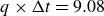 $q\times \Delta t=9.08$
; (
$q\times \Delta t=9.08$
; (
 $b$
)
$b$
)
 $q\times \Delta t=13.62$
; (
$q\times \Delta t=13.62$
; (
 $c$
)
$c$
)
 $q\times \Delta t=18.16$
.
$q\times \Delta t=18.16$
.

There is another important observation that we can make by inspecting figure 18. The performance of reconstruction from a small number of sensors (even one sensor) improves significantly as the time delay
 $q \times \Delta t$
grows; compare for example FIT[
$q \times \Delta t$
grows; compare for example FIT[
 $\%$
] across the three values of
$\%$
] across the three values of
 $q \times \Delta t$
when
$q \times \Delta t$
when
 $n_p=1$
sensor is used. Especially for the largest time delay, adding more sensors only marginally increases the FIT[
$n_p=1$
sensor is used. Especially for the largest time delay, adding more sensors only marginally increases the FIT[
 $\%$
] values. This trend agrees with the findings of Takens (Reference Takens1981) who recognised the usefulness of time-delayed embeddings of even a single observable for the analysis of chaotic systems.
$\%$
] values. This trend agrees with the findings of Takens (Reference Takens1981) who recognised the usefulness of time-delayed embeddings of even a single observable for the analysis of chaotic systems.
Figures 19 and 20 depict the reconstruction of time coefficients of the six dominant POD modes in the training dataset and the future evolution in the forecasting dataset for the two largest time widows
 $q \times \Delta t=13.62 \text{ and }18.16$
, respectively. The process to obtain these figures is as follows. Velocity measurements
$q \times \Delta t=13.62 \text{ and }18.16$
, respectively. The process to obtain these figures is as follows. Velocity measurements
 ${\boldsymbol{s}}[k]$
at
${\boldsymbol{s}}[k]$
at
 $n_{p}$
points are employed to estimate the time coefficients
$n_{p}$
points are employed to estimate the time coefficients
 ${\boldsymbol{a}}[k]$
from
${\boldsymbol{a}}[k]$
from
 $k=0 \ldots K_{\textit{train}}$
. At
$k=0 \ldots K_{\textit{train}}$
. At
 $k=K_{\textit{train}}$
, the estimation is extended from
$k=K_{\textit{train}}$
, the estimation is extended from
 $k_{{\textit{train}}+1} \ldots K_{\textit{train}}+q$
. Given the three-dimensional turbulent nature of the flow, the forecasting quality of the first two dominant modes is impressive. Both the amplitude and phase are well predicted even for the largest time delay (which is more than two orders of magnitude larger than the Lyapunov time scale). The slowly evolving third mode is also well forecast. Small discrepancies are detected in the higher modes, but again the phase and amplitude are satisfactorily reproduced especially for the largest time window. Recall that modes
$k_{{\textit{train}}+1} \ldots K_{\textit{train}}+q$
. Given the three-dimensional turbulent nature of the flow, the forecasting quality of the first two dominant modes is impressive. Both the amplitude and phase are well predicted even for the largest time delay (which is more than two orders of magnitude larger than the Lyapunov time scale). The slowly evolving third mode is also well forecast. Small discrepancies are detected in the higher modes, but again the phase and amplitude are satisfactorily reproduced especially for the largest time window. Recall that modes
 $4{-}6$
have very little energy, in the range
$4{-}6$
have very little energy, in the range
 $(1{-}2)\,\%$
as shown in figure 9, so these deviations are not surprising. The estimated
$(1{-}2)\,\%$
as shown in figure 9, so these deviations are not surprising. The estimated
 ${\boldsymbol{a}}[k]$
between
${\boldsymbol{a}}[k]$
between
 $k=K_{\textit{train}}-q \ldots K_{\textit{train}}$
(region between dashed and solid lines) slightly deviates from the ground truth, probably because this is the last column in the Hankel matrix
$k=K_{\textit{train}}-q \ldots K_{\textit{train}}$
(region between dashed and solid lines) slightly deviates from the ground truth, probably because this is the last column in the Hankel matrix
 $\boldsymbol{H}$
. These small deviations are more pronounced for modes
$\boldsymbol{H}$
. These small deviations are more pronounced for modes
 $4{-}6$
and also propagate inside the forecasting window affecting the accuracy. Note that we obtained the results of figures 19 and 20 using the correct initial value of
$4{-}6$
and also propagate inside the forecasting window affecting the accuracy. Note that we obtained the results of figures 19 and 20 using the correct initial value of
 $\boldsymbol{\hat {v}}_{H}[0]$
(for this reason the blue and red lines match at t = 0). However, this is not a restriction. If the value of
$\boldsymbol{\hat {v}}_{H}[0]$
(for this reason the blue and red lines match at t = 0). However, this is not a restriction. If the value of
 $\boldsymbol{\hat {v}}_{H}[0]$
is not known, it can be set as 0. In this case,
$\boldsymbol{\hat {v}}_{H}[0]$
is not known, it can be set as 0. In this case,
 $\boldsymbol{\hat {v}}_{H}[k]$
will be updated as streaming data
$\boldsymbol{\hat {v}}_{H}[k]$
will be updated as streaming data
 ${\boldsymbol{s}}[k]$
are coming in, and the estimated
${\boldsymbol{s}}[k]$
are coming in, and the estimated
 $\hat {a}_i[k]$
will take some time to catch up with the true solution
$\hat {a}_i[k]$
will take some time to catch up with the true solution
 $a_i[k]$
.
$a_i[k]$
.
Forecasting of the future evolution of the POD coefficients using velocity measurements for
 $q\times \Delta t=13.62$
with
$q\times \Delta t=13.62$
with
 $m_u=68$
,
$m_u=68$
,
 $n_{p}=63$
. The solid vertical line indicates the starting point of the forecasting dataset. The time window between the dashed and solid lines marks
$n_{p}=63$
. The solid vertical line indicates the starting point of the forecasting dataset. The time window between the dashed and solid lines marks
 $t_{p}$
to
$t_{p}$
to
 $t_{Ktrain}$
, which is the time extent of the last column of the Hankel matrix
$t_{Ktrain}$
, which is the time extent of the last column of the Hankel matrix
 $\boldsymbol{H}$
. Blue lines indicate DNS and red lines reconstruction/forecasting.
$\boldsymbol{H}$
. Blue lines indicate DNS and red lines reconstruction/forecasting.

Forecasting of the future evolution of the POD coefficients using velocity measurements for
 $q\times \Delta t=18.16$
with
$q\times \Delta t=18.16$
with
 $m_u=37$
,
$m_u=37$
,
 $n_{p}=14$
. Blue lines indicate DNS and red lines reconstruction/forecasting. For the meaning of the vertical dashed and solid lines, refer to the caption of figure 19.
$n_{p}=14$
. Blue lines indicate DNS and red lines reconstruction/forecasting. For the meaning of the vertical dashed and solid lines, refer to the caption of figure 19.

4.5. Flow-field reconstruction and forecasting from scalar measurements
We now turn our attention to the forecasting of the velocity field from scalar measurements. Recall that we place the scalar sensors at the peaks of the POD velocity modes, but they record only one piece of information, the concentration.
In figure 21, we explore the effect of the number of velocity and scalar POD modes
 $m_u$
and
$m_u$
and
 $m_c$
, respectively, and the number of measurements
$m_c$
, respectively, and the number of measurements
 $n_{p}$
on the FIT[
$n_{p}$
on the FIT[
 $\%$
] metric for the same values of time-delayed snapshots
$\%$
] metric for the same values of time-delayed snapshots
 $q$
as in figure 18. It can be seen that now larger values of
$q$
as in figure 18. It can be seen that now larger values of
 $m_u$
and
$m_u$
and
 $m_c$
are required for the results to converge. As in the case of velocity measurements, FIT[
$m_c$
are required for the results to converge. As in the case of velocity measurements, FIT[
 $\%$
] is reduced, but only slightly, as
$\%$
] is reduced, but only slightly, as
 $q$
increases. Again this is a positive result that demonstrates that one can robustly forecast the velocity field from scalar measurements which are more cost effective to obtain. The FIT[
$q$
increases. Again this is a positive result that demonstrates that one can robustly forecast the velocity field from scalar measurements which are more cost effective to obtain. The FIT[
 $\%$
] values are slightly smaller compared with the results of the previous section. Most likely this is because the sensors record only the scalar concentration, i.e. they provide less information to the estimator. The performance of reconstruction from a small number of sensors again improves as the time delay
$\%$
] values are slightly smaller compared with the results of the previous section. Most likely this is because the sensors record only the scalar concentration, i.e. they provide less information to the estimator. The performance of reconstruction from a small number of sensors again improves as the time delay
 $q \times \Delta t$
grows, but the improvement is not as clear as when velocity sensors are used.
$q \times \Delta t$
grows, but the improvement is not as clear as when velocity sensors are used.
The FIT[
 $\%$
] metric against the number of scalar sensors,
$\%$
] metric against the number of scalar sensors,
 $n_{p}$
: (
$n_{p}$
: (
 $a$
)
$a$
)
 $q\times \Delta t=9.08$
; (
$q\times \Delta t=9.08$
; (
 $b$
)
$b$
)
 $q\times \Delta t=13.62$
; (
$q\times \Delta t=13.62$
; (
 $c$
)
$c$
)
 $q\times \Delta t=18.16$
.
$q\times \Delta t=18.16$
.

In figure 22 we plot the reconstructed and forecast time series of the first six POD modes from scalar measurements for the largest
 $q\times \Delta t=18.16$
. Again, the time signals closely follow the true ones in the training dataset. In the forecasting dataset, the model predicts the first three time coefficients very well. The quality is comparable to that of figure 20 where velocity sensors are used. These plots demonstrate that it is possible to get accurate results from scalar measurements.
$q\times \Delta t=18.16$
. Again, the time signals closely follow the true ones in the training dataset. In the forecasting dataset, the model predicts the first three time coefficients very well. The quality is comparable to that of figure 20 where velocity sensors are used. These plots demonstrate that it is possible to get accurate results from scalar measurements.
Forecasting of the future evolution of the dominant POD coefficients using scalar measurements for
 $q\times \Delta t=18.16$
with
$q\times \Delta t=18.16$
with
 $m_u=115$
,
$m_u=115$
,
 $m_c=75$
and
$m_c=75$
and
 $n_{p}=123$
.
$n_{p}=123$
.

5. Conclusions
A data-driven estimator was synthesised that can forecast the future evolution of a three-dimensional turbulent flow field from current sparse velocity and/or scalar measurements. This is made possible by combining time-delayed embedding, Koopman theory and optimal estimation theory. The key idea is the construction of a linear dynamical system that governs the future POD coefficients and closure of the system using sensor measurements.
The estimator was applied to the three-dimensional turbulent recirculating flow around a surface-mounted cube. Velocity (and scalar, if required) sensors were placed at the peaks of the velocity POD modes. Forecasting the future evolution of the dominant POD modes was performed over time windows one to two orders of magnitude larger than the Lyapunov time scale. Accurate forecasting was obtained for the first three velocity POD modes. Results with velocity sensors were slightly more accurate compared with scalar sensors. The forecasting accuracy only slightly decreased as the window size increased. This was true for both velocity and scalar sensors. The results demonstrate that long forecasts can be made for the most dominant structures of the flow.
The method can be extended to include other dimensionality reduction techniques, for example convolutional autoencoders. This will allow more compact representation of the dynamics, which is especially useful for high-Reynolds-number flows. The resulting nonlinearity of the mapping between the latent space variables and the velocity field can be dealt with using other estimators, such as the ensemble Kalman filter. Application of the method to other flow settings, such as wall-bounded flows using pressure and/or shear stress measurements, would be particularly interesting. The framework can also easily incorporate data from moving sensors, such as drones or wearable sensors. Another extension is to train at different operating conditions (e.g. different Reynolds members) and forecast the flow at an unseen condition using only streaming data from the new condition.
Acknowledgements
The authors would like to thank EPSRC for the computational time made available on the UK supercomputing facility ARCHER/ARCHER2 via the UK Turbulence Consortium (EP/X035484/1).
Funding
G.P. is supported by EPSRC grants EP/X017273/1 and EP/W001748/1.
Declaration of interests
The authors report no conflict of interest.
Author contributions
Both authors contributed equally to analysing data and reaching conclusions, and in writing the paper.


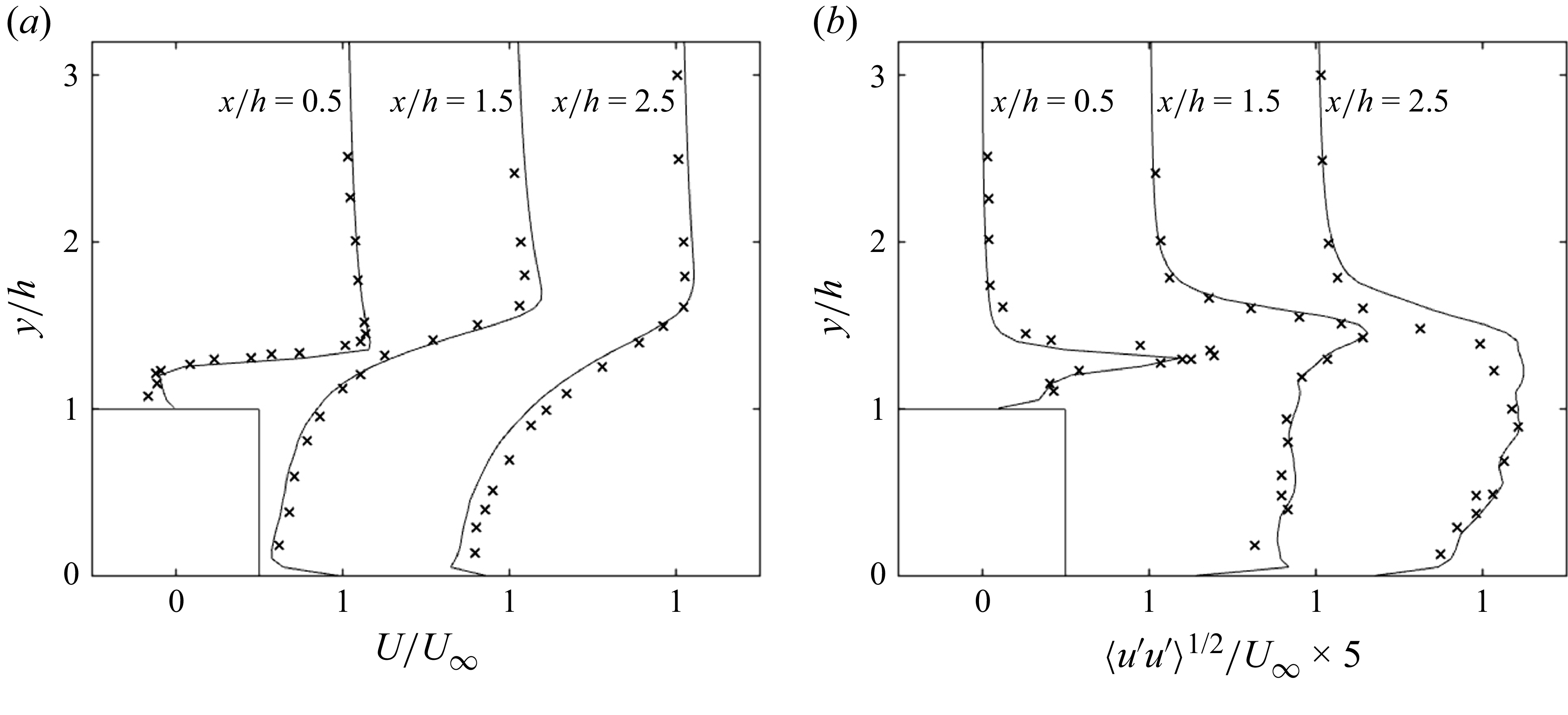


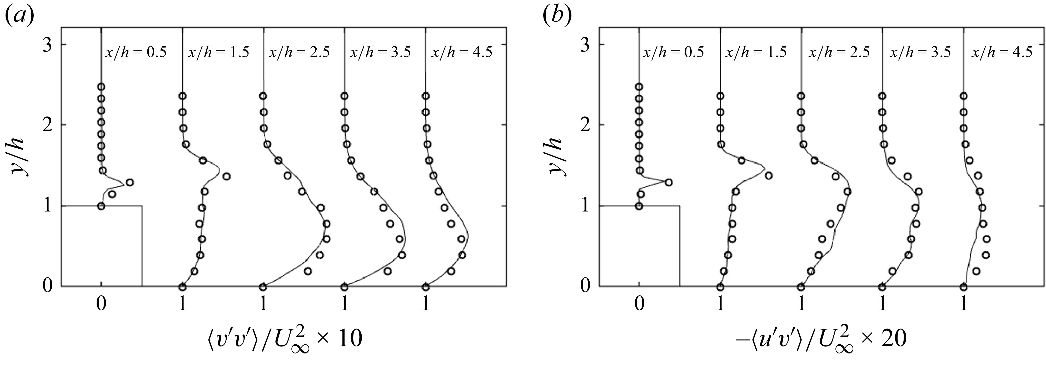


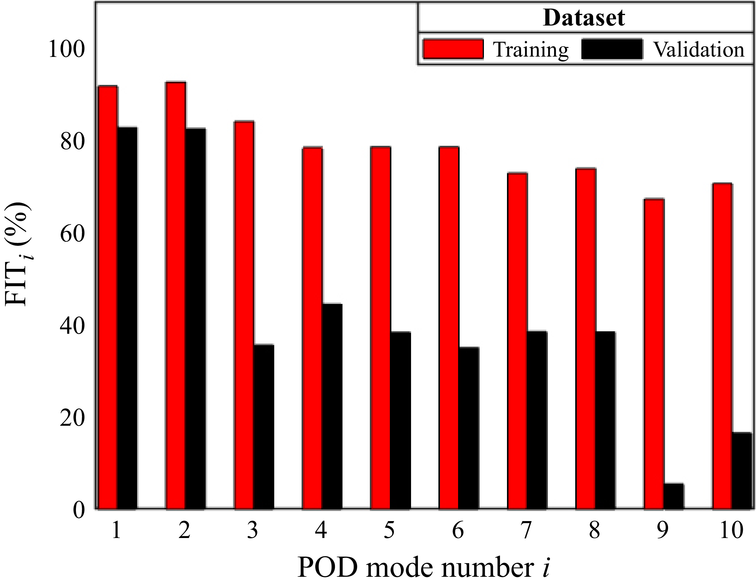


 Open access