




1 Introduction
High-energy gamma-ray spectroscopy in the multi-MeV to GeV range is essential for advancing our understanding of fundamental physics and emerging applications, from astrophysics to strong-field quantum electrodynamics (SFQED). Despite significant progress in gamma-ray source development, such as bremsstrahlung emission from laser-wakefield accelerated electron beams[ Reference Li, Li, Ju, Jiang, Yu, Huang, Zhang, Wu, Qiao, Zhou and He 1 – Reference Lemos, King, Rusby, Pagano, Sinclair, Marsh, Shaw, Milder, Pak, Pollock, Aufderheide, Hartemann, Wu, Hwang, Hegelich, Moody, Michel, Joshi and Albert 4 ] and inverse Compton scattering[ Reference Sarri, Corvan, Schumaker, Cole, Di Piazza, Ahmed, Harvey, Keitel, Krushelnick, Mangles, Najmudin, Symes, Thomas, Yeung, Zhao and Zepf 5 – Reference Mirzaie, Hojbota, Kim, Pathak, Pak, Kim, Lee, Yoon, Lee, Rhee, Vranic, Amaro, Kim, Sung and Nam 8 ], precise spectral reconstruction of high-flux gamma-ray beams remains a challenge. The filter-stacked spectrometer consists of multiple filter layers and a recording medium, commonly used for detecting hard X-rays and gamma rays in the range from several to tens of MeV[ Reference Nolte, Behrens, Schnürer, Rousse and Ambrosi 9 – Reference Behrens 12 ]. However, its spectral resolution is very low in the tens of MeV to even GeV energy range. Recent studies have demonstrated[ Reference Schumaker, Sarri, Vargas, Zhao, Behm, Chvykov, Dromey, Hou, Maksimchuk, Nees, Yanovsky, Zepf, Thomas and Krushelnick 13 – Reference Singh, Versaci, Garcia, Morejon, Ferrari, Molodtsova, Schwengner, Kumar and Cowan 15 ] that gamma-ray spectrometers can be developed by analyzing secondary particle energy spectra resulting from gamma-ray interactions with a converter medium.
For instance, Compton scattering in low-Z materials has been used to convert gamma-ray energy into measurable electron spectra[ Reference Corvan, Sarri and Zepf 16 – Reference Naranjo, Andonian, Fukasawa, Lynn, Majernik, Rosenzweig, Sakai, Williams, Yadav and Zhuang 20 ], enabling gamma-ray detection in the 0.5–30 MeV range with compact magnetic systems and detectors. At higher energies, pair spectrometers[ Reference Fleck, Cavanagh and Sarri 21 – Reference Song, Noh, Mirzaie, Hojbota, Kim, Lee, Won, Song and Bang 24 ] based on the pair production process in high-Z materials (e.g., tungsten, lead) have been proposed. These spectrometers convert gamma-rays into electron–positron pairs, with the original spectra reconstructed by analyzing the energy and momentum distributions of the pairs with a magnetic spectrometer. The primary focus is on the precise measurement of high-energy gamma rays, reaching GeV or even 10 GeV levels. The converter thickness is crucial for the accurate measurement of the energy spectrum. Techniques using thin converters to suppress multiple scattering offer advantages in high-flux scenarios[ Reference Abramowicz, Almanza Soto, Altarelli, Aßmann, Athanassiadis, Avoni, Behnke, Benettoni, Benhammou, Bhatt, Blackburn, Blanch, Bonaldo, Boogert, Borysov, Borysova, Boudry, Breton, Brinkmann, Bruschi, Burkart, Büßer, Cavanagh, Dal Corso, Decking, Deniaud, Diner, Dosselli, Elad, Epshteyn, Esperante, Ferber, Firlej, Fiutowski, Fleck, Fuster-Martinez, Gadow, Gaede, Gallas, Garcia Cabrera, Gerstmayr, Ghenescu, Giorato, Golubeva, Grojean, Grutta, Grzelak, Hallford, Hartman, Heinemann, Heinzl, Helary, Hendriks, Hoffmann, Horn, Huang, Huang, Idzik, Irles, Jacobs, King, Klute, Kropf, Kroupp, Lahno, Lasagni Manghi, Lawhorn, Levanon, Levi, Levinson, Levy, Levy, Liberman, Liss, List, List, Lohmann, Maalmi, Madlener, Malka, Marsault, Mattiazzo, Meloni, Miron, Morandin, Moron, Nanni, Neagu, Negodin, Paccagnella, Pantano, Pietruch, Pomerantz, Pöschl, Potlog, Prasad, Quishpe, Ranken, Ringwald, Roich, Salgado, Santra, Sarri, Sävert, Sbrizzi, Schmitt, Schulthess, Schuwalow, Seipt, Simi, Soreq, Spataro, Streeter, Swientek, Tal Hod, Teter, Thiebault, Thoden, Trevisani, Urmanov, Vasiukov, Walker, Warren, Wing, Yap, Zadok, Zanetti, Zarnecki, Zbinkowski, Zembaczynski, Zepf, Zerwas, Ziegler and Zuffa 23 ]. However, many experiments still require thicker converters during operation because they are advantageous or indispensable under certain conditions. In unknown-flux or single-shot experiments, thicker converters are often employed to increase the reaction probability, leading to higher positron or electron yields, despite introducing more complex energy degradation. The choice of converter thickness thus involves a trade-off between resolution and yield, depending on the photon flux and the specific diagnostic requirements[ Reference Corvan, Sarri and Zepf 16 ]. This has created a demand for spectrometer design and reconstruction algorithms.
Several traditional algorithms, including iterative reconstruction[ Reference Kim and Lee 25 ], Tikhonov regularization[ Reference Zhang, Yang, Hu, Li, Luo, An and Zheng 17 ] and maximum likelihood estimation (MLE)[ Reference Lowell, Boggs, Chiu, Kierans, Sleator, Tomsick, Zoglauer, Chang, Tseng, Yang, Jean, Ballmoos, Lin and Amman 26 ], are effective for Compton spectrometers. However, they provide only approximate solutions for the spectra of GeV gamma rays. The statistical Bayesian approach[ Reference Cavanagh, Fleck, Streeter, Gerstmayr, Dickson, Ballage, Cadas, Calvin, Dufrénoy, Moulanier, Romagnani, Vasilovici, Whitehead, Specka, Cros and Sarri 22 , Reference D’Agostini 27 , 28 ] and machine learning methods such as fully connected networks[ Reference Yadav, Oruganti, Naranjo, Andonian, Apsimon, Welsch and Rosenzweig 29 ] have been explored for reconstruction in the GeV range. It is envisioned that the statistical Bayesian algorithm can be further improved by combining the Bayesian nature of this method with machine learning techniques[ Reference Fleck 30 ]. Fully connected neural networks, with their simple architectures, struggle to capture complex features such as nonlinear Compton scattering and laser-wakefield acceleration (LWFA)-driven strong bremsstrahlung gamma rays in the presence of high noise, leaving room for improvement.
Here, we present an approach for gamma-ray spectroscopy that combines a spectrometer design with a corresponding machine learning approach for extracting photon energy spectra. Building upon the geometric structure of gamma-ray spectrometers, we frame spectral reconstruction as a high-dimensional inverse problem, developing a data-driven framework that outperforms traditional regularization techniques in both accuracy and applicability. Using Monte Carlo (MC) simulations, we quantify the energy-dependent response of the spectrometer system to incident photons. We introduce an end-to-end machine learning network architecture, consisting of a denoising autoencoder (DAE) and a reconstruction U-Net, to effectively separate overlapping cascade features while preserving physical consistency.
The paper is organized as follows. Section 2 outlines the spectrometer design and parameter optimization. The gamma-ray energy spectrum extraction procedure is described in Section 3. The comparison and evaluation of reconstruction results are presented in Section 4. Finally, Section 5 concludes the study and provides an outlook on future developments.
2 Design of the spectrometer
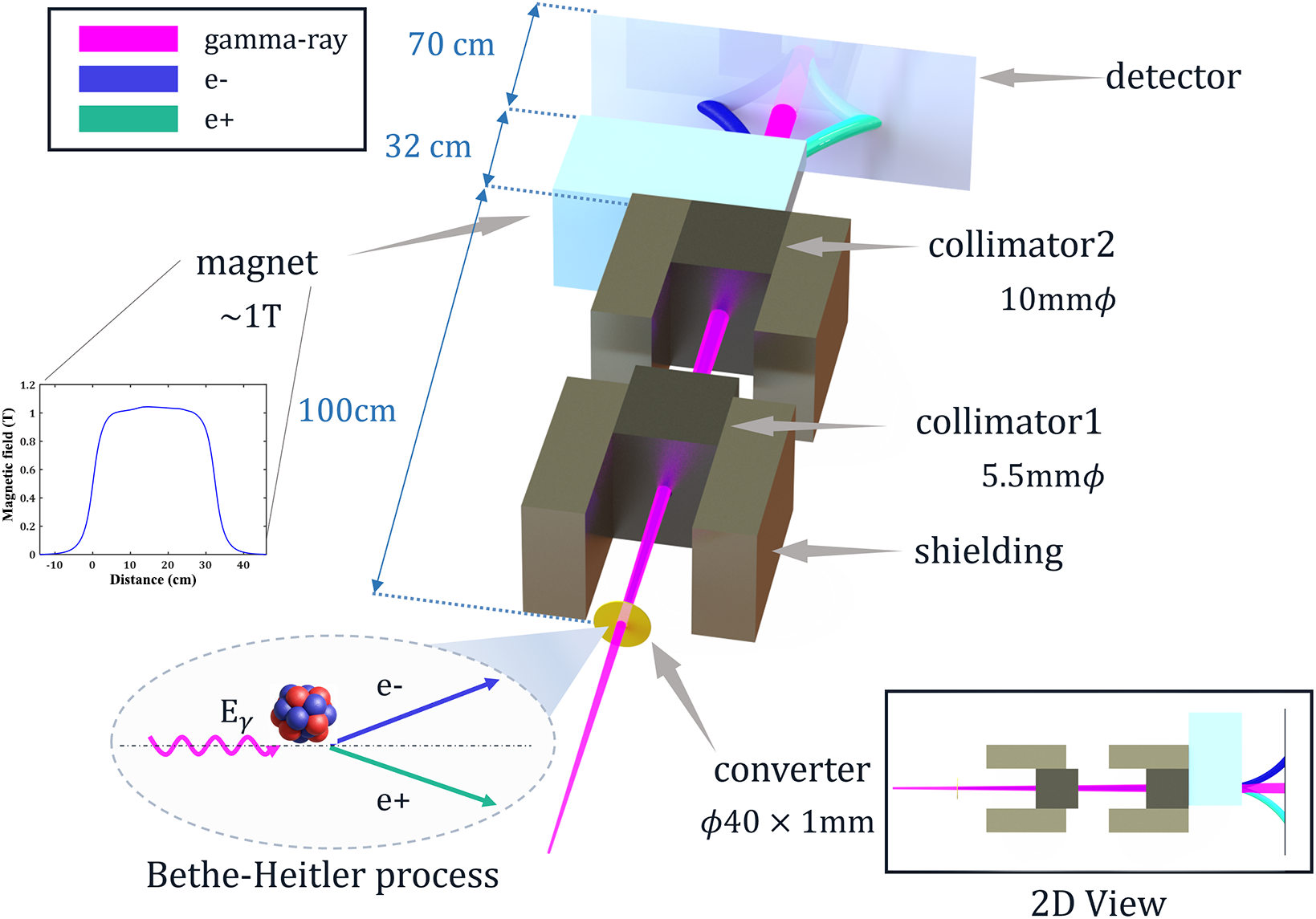
The overall mechanical structure of the spectrometer is shown in Figure 1. The spectrometer consists of three components: the converter, the collimator and the pair magnet spectrometer. The converter converts a small percentage of the incident high-energy photons into electron–positron pairs[ Reference Fleck, Cavanagh and Sarri 21 ], and the collimated aperture shields the system from major noise (e.g., off-axis photons and low-energy electrons). The electron–positron pairs are collected by detectors symmetrically distributed around the magnetic spectrometer. The double collimator configuration has proven to be ideal[ Reference Fleck, Cavanagh and Sarri 21 , Reference Song, Noh, Mirzaie, Hojbota, Kim, Lee, Won, Song and Bang 24 ] for minimizing the background on the detector when measuring GeV-scale electron–positron pairs.
Schematic layout of the GeV-scale gamma-ray spectrometer. An ultra-short gamma-ray pulse interacts with a 1 mm thick tungsten converter to generate electron–positron pairs via the Bethe–Heitler (BH) process. Then, the pairs traverse the double collimator before being spatially separated by a dipole magnet and recorded on the detector plane. The two-dimensional top view (bottom-right inset) illustrates the top view of the spectrometer components. The distances between components are optimized for energy resolution.

The gamma-ray spectrometer is based on the process of pair production in a nuclear field. Neglecting the recoil energy of the nucleus, an electron–positron pair may be produced in the Coulomb field of the nucleus only after the photon energy exceeds the rest mass of the pair by $2{m}_\mathrm{e}{c}^2$
, where
$2{m}_\mathrm{e}{c}^2$
, where ${m}_\mathrm{e}$
is the rest mass of the electron and
${m}_\mathrm{e}$
is the rest mass of the electron and $c$
is the speed of light. As photon energy increases, pair production begins to dominate photon–matter interactions above approximately 50 MeV, overtaking Compton scattering as the primary process in high-Z materials[
Reference Corvan, Sarri and Zepf
16
]. In the ultra-relativistic approximation, the total cross-section[
Reference Fleck, Cavanagh and Sarri
21
, Reference Berestetskii, Pitaevskii and Lifshitz
31
] for pair production in the nuclear field can be expressed as follows:
$c$
is the speed of light. As photon energy increases, pair production begins to dominate photon–matter interactions above approximately 50 MeV, overtaking Compton scattering as the primary process in high-Z materials[
Reference Corvan, Sarri and Zepf
16
]. In the ultra-relativistic approximation, the total cross-section[
Reference Fleck, Cavanagh and Sarri
21
, Reference Berestetskii, Pitaevskii and Lifshitz
31
] for pair production in the nuclear field can be expressed as follows:
 $$\begin{align}\sigma \approx \frac{28}{9}\alpha {Z}^2{r}_\mathrm{e}^2\left[\log \left(\frac{2{E}_{\gamma }}{m_\mathrm{e}{c}^2}\right)-\frac{109}{42}\right],\end{align}$$
where $\alpha \approx$
1/137 is the fine-structure constant,
$\alpha \approx$
1/137 is the fine-structure constant, ${r}_\mathrm{e}$
is the classical electron radius and
${r}_\mathrm{e}$
is the classical electron radius and $Z$
is the atomic number of the converter material.
$Z$
is the atomic number of the converter material.
Due to additional processes in the converter that may cause electron generation or scattering, the electron spectrum is typically affected by higher noise levels on the detector plane[
Reference Cavanagh, Fleck, Streeter, Gerstmayr, Dickson, Ballage, Cadas, Calvin, Dufrénoy, Moulanier, Romagnani, Vasilovici, Whitehead, Specka, Cros and Sarri
22
]. Therefore, it is preferable to pay attention to the positrons and maximize their yield. The yield of high-energy positrons generated via the Bethe–Heitler process is proportional to the product of the pair production cross-section and the number density of the target nucleus ${N}_\mathrm{A}\rho /M$
, where
${N}_\mathrm{A}\rho /M$
, where ${N}_\mathrm{A}$
is Avogadro’s constant,
${N}_\mathrm{A}$
is Avogadro’s constant, $\rho$
is the material density and
$\rho$
is the material density and $M$
is the molar mass. Equation (1) shows that the pair production cross-section is proportional to the square of the atomic number of the target nucleus. Therefore, to maximize the probability of pair production and consequently the yield of measurable positrons, it is necessary to select materials with high atomic numbers as target materials. Typically, high-Z elements suitable for target materials include gold, tungsten, tantalum and lead. According to theoretical calculations, the gold target had the highest
$M$
is the molar mass. Equation (1) shows that the pair production cross-section is proportional to the square of the atomic number of the target nucleus. Therefore, to maximize the probability of pair production and consequently the yield of measurable positrons, it is necessary to select materials with high atomic numbers as target materials. Typically, high-Z elements suitable for target materials include gold, tungsten, tantalum and lead. According to theoretical calculations, the gold target had the highest ${Z}^2{N}_\mathrm{A}\rho /M$
value among the four metal targets mentioned before. Thus, gold produced the highest positron yield, followed by tungsten. To study the energy spectrum of positrons after a 1 GeV monoenergetic gamma-ray beam passes through different 500 μm thick materials, simulations are performed using the MC particle tracking code Geant4[
Reference Agostinelli, Allison, Amako, Apostolakis, Araujo, Arce, Asai, Axen, Banerjee, Barrand, Behner, Bellagamba, Boudreau, Broglia, Brunengo, Burkhardt, Chauvie, Chuma, Chytracek, Cooperman, Cosmo, Degtyarenko, Dell'Acqua, Depaola, Dietrich, Enami, Feliciello, Ferguson, Fesefeldt, Folger, Foppiano, Forti, Garelli, Giani, Giannitrapani, Gibin, Gómez Cadenas, González, Gracia Abril, Greeniaus, Greiner, Grichine, Grossheim, Guatelli, Gumplinger, Hamatsu, Hashimoto, Hasui, Heikkinen, Howard, Ivanchenko, Johnson, Jones, Kallenbach, Kanaya, Kawabata, Kawabata, Kawaguti, Kelner, Kent, Kimura, Kodama, Kokoulin, Kossov, Kurashige, Lamanna, Lampén, Lara, Lefebure, Lei, Liendl, Lockman, Longo, Magni, Maire, Medernach, Minamimoto, Mora de Freitas, Morita, Murakami, Nagamatu, Nartallo, Nieminen, Nishimura, Ohtsubo, Okamura, O'Neale, Oohata, Paech, Perl, Pfeiffer, Pia, Ranjard, Rybin, Sadilov, Di Salvo, Santin, Sasaki, Savvas, Sawada, Scherer, Sei, Sirotenko, Smith, Starkov, Stoecker, Sulkimo, Takahata, Tanaka, Tcherniaev, Safai Tehrani, Tropeano, Truscott, Uno, Urban, Urban, Verderi, Walkden, Wander, Weber, Wellisch, Wenaus, Williams, Wright, Yamada, Yoshida and Zschiesche
32
]. Our simulation utilizes the physics package QGSP_BERT
[
Reference Song, Kim, Won, Song, Lee, Ryu, Bang and Nam
33
], which incorporates energy loss processes for electrons and positrons, including bremsstrahlung, Coulomb scattering and ionization. We assume pencil-shaped photon beams with no initial divergence in our simulations and positron signals are directly collected behind the target. Table 1 and Figure 2(a) show the
${Z}^2{N}_\mathrm{A}\rho /M$
value among the four metal targets mentioned before. Thus, gold produced the highest positron yield, followed by tungsten. To study the energy spectrum of positrons after a 1 GeV monoenergetic gamma-ray beam passes through different 500 μm thick materials, simulations are performed using the MC particle tracking code Geant4[
Reference Agostinelli, Allison, Amako, Apostolakis, Araujo, Arce, Asai, Axen, Banerjee, Barrand, Behner, Bellagamba, Boudreau, Broglia, Brunengo, Burkhardt, Chauvie, Chuma, Chytracek, Cooperman, Cosmo, Degtyarenko, Dell'Acqua, Depaola, Dietrich, Enami, Feliciello, Ferguson, Fesefeldt, Folger, Foppiano, Forti, Garelli, Giani, Giannitrapani, Gibin, Gómez Cadenas, González, Gracia Abril, Greeniaus, Greiner, Grichine, Grossheim, Guatelli, Gumplinger, Hamatsu, Hashimoto, Hasui, Heikkinen, Howard, Ivanchenko, Johnson, Jones, Kallenbach, Kanaya, Kawabata, Kawabata, Kawaguti, Kelner, Kent, Kimura, Kodama, Kokoulin, Kossov, Kurashige, Lamanna, Lampén, Lara, Lefebure, Lei, Liendl, Lockman, Longo, Magni, Maire, Medernach, Minamimoto, Mora de Freitas, Morita, Murakami, Nagamatu, Nartallo, Nieminen, Nishimura, Ohtsubo, Okamura, O'Neale, Oohata, Paech, Perl, Pfeiffer, Pia, Ranjard, Rybin, Sadilov, Di Salvo, Santin, Sasaki, Savvas, Sawada, Scherer, Sei, Sirotenko, Smith, Starkov, Stoecker, Sulkimo, Takahata, Tanaka, Tcherniaev, Safai Tehrani, Tropeano, Truscott, Uno, Urban, Urban, Verderi, Walkden, Wander, Weber, Wellisch, Wenaus, Williams, Wright, Yamada, Yoshida and Zschiesche
32
]. Our simulation utilizes the physics package QGSP_BERT
[
Reference Song, Kim, Won, Song, Lee, Ryu, Bang and Nam
33
], which incorporates energy loss processes for electrons and positrons, including bremsstrahlung, Coulomb scattering and ionization. We assume pencil-shaped photon beams with no initial divergence in our simulations and positron signals are directly collected behind the target. Table 1 and Figure 2(a) show the ${Z}^2\rho /M$
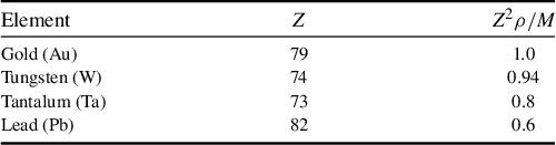
value and the normalized positron energy spectra produced by a 1 GeV monoenergetic gamma-ray beam propagating through 500 μm thick layers of different target materials. The simulation results are consistent with the numerical estimates. We chose tungsten as the converter material because of its sustainability compared to gold.
${Z}^2\rho /M$
value and the normalized positron energy spectra produced by a 1 GeV monoenergetic gamma-ray beam propagating through 500 μm thick layers of different target materials. The simulation results are consistent with the numerical estimates. We chose tungsten as the converter material because of its sustainability compared to gold.
Atomic number and normalized parameter ( ${Z}^2\rho /M$
) for different target materials. This parameter is proportional to the theoretical positron yield per incident gamma-ray photon. The parameters are normalized with the value of gold as the maximum value for the sake of comparison.
${Z}^2\rho /M$
) for different target materials. This parameter is proportional to the theoretical positron yield per incident gamma-ray photon. The parameters are normalized with the value of gold as the maximum value for the sake of comparison.

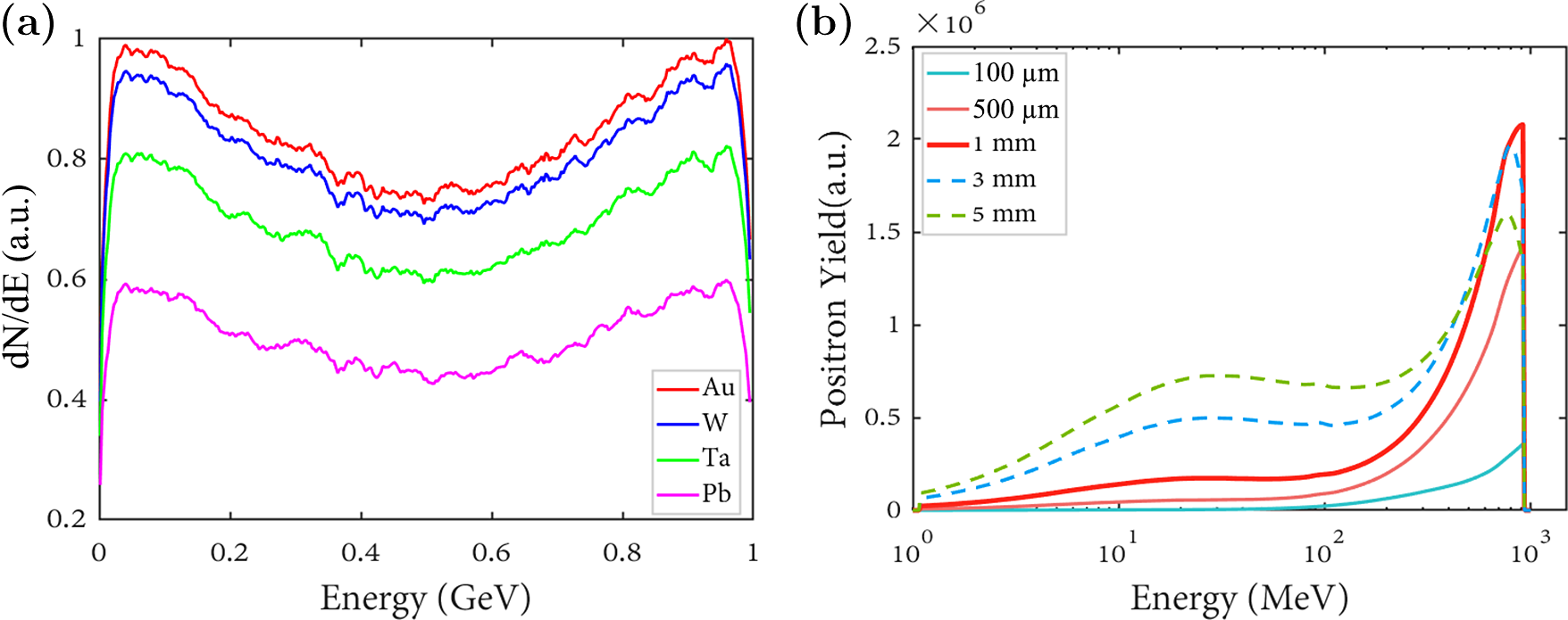
Optimization of the converter for a 1 GeV monoenergetic gamma-ray beam. (a) Effect of material: normalized positron energy spectra for different 500 μm thick materials (Au, W, Ta and Pb) recorded directly behind the converter. (b) Effect of thickness: positron yield for tungsten targets of varying thicknesses (100 μm, 500 μm, 1 mm, 3 mm, 5 mm) measured behind the collimated aperture. The x-axis represents the energy of the generated positrons (in logarithmic scale), and the y-axis shows the positron yield per energy bin. As the tungsten layer thickness increases, the spectral line peak begins to decrease after reaching its maximum value at 1 mm.

The relationship between converter thickness and yield[
Reference Weng, Tan, Hei, Zhang, Sun, Wei and Liu
34
] is a key factor in optimizing spectrometers. In our simulation, a ${10}^8$
pencil-shaped monoenergetic gamma-ray beam with an energy of 1 GeV was simulated penetrating tungsten targets of thicknesses 100 μm, 500 μm, 1 mm, 3 mm and 5 mm. A divergent gamma-ray beam will increase the divergence of the electron–positron pairs and thus reduce the spectral resolution of the system. We add a 5 mm collimated aperture behind the target to minimize the secondary-effect tails of tens of MeV and collect positron signals from the rear of the collimator. Figure 2(b) shows the positron yield as a function of energy for tungsten targets with different thicknesses. A key parameter to define in this figure is the size of the energy bin corresponding to the number of positrons. It is not meaningful to select an energy bin size smaller than the spectrometer’s intrinsic energy resolution (see Equation (2)). The advantage of this binning method is that it allows the optimal converter thickness to be selected based on the full width at half maximum (FWHM) of the positron yield distribution. As shown in the figure, the spectral broadening arises largely from the scattering of positrons as they pass through the converter. Hence, there is a compromise between spectral resolution and yield. As the tungsten layer thickness increases, the FWHM of the energy spectrum gradually broadens. However, the spectral peak in the high-energy region does not present a single increasing trend; instead, an optimal peak exists. It is worth noting that the radiation length of tungsten is 3.5 mm[
Reference Navas
35
]. For millimeter-thick target materials, the thickness is comparable to the radiation length, requiring careful selection of thicknesses exceeding the radiation length. The thickness of tungsten depends largely on the photon flux to be investigated. A 1 mm tungsten converter thickness provides the optimal balance between positron yield and energy resolution, minimizing spectral broadening while ensuring sufficient signal intensity. For our application, a compromise thickness of 1 mm can be selected.
${10}^8$
pencil-shaped monoenergetic gamma-ray beam with an energy of 1 GeV was simulated penetrating tungsten targets of thicknesses 100 μm, 500 μm, 1 mm, 3 mm and 5 mm. A divergent gamma-ray beam will increase the divergence of the electron–positron pairs and thus reduce the spectral resolution of the system. We add a 5 mm collimated aperture behind the target to minimize the secondary-effect tails of tens of MeV and collect positron signals from the rear of the collimator. Figure 2(b) shows the positron yield as a function of energy for tungsten targets with different thicknesses. A key parameter to define in this figure is the size of the energy bin corresponding to the number of positrons. It is not meaningful to select an energy bin size smaller than the spectrometer’s intrinsic energy resolution (see Equation (2)). The advantage of this binning method is that it allows the optimal converter thickness to be selected based on the full width at half maximum (FWHM) of the positron yield distribution. As shown in the figure, the spectral broadening arises largely from the scattering of positrons as they pass through the converter. Hence, there is a compromise between spectral resolution and yield. As the tungsten layer thickness increases, the FWHM of the energy spectrum gradually broadens. However, the spectral peak in the high-energy region does not present a single increasing trend; instead, an optimal peak exists. It is worth noting that the radiation length of tungsten is 3.5 mm[
Reference Navas
35
]. For millimeter-thick target materials, the thickness is comparable to the radiation length, requiring careful selection of thicknesses exceeding the radiation length. The thickness of tungsten depends largely on the photon flux to be investigated. A 1 mm tungsten converter thickness provides the optimal balance between positron yield and energy resolution, minimizing spectral broadening while ensuring sufficient signal intensity. For our application, a compromise thickness of 1 mm can be selected.
In order to study the overall performance of the spectrometer, Figure 3 shows the two-dimensional particle distribution of ${10}^7$
photons propagating through the gamma-ray spectrometer simulated using the FLUKA code[
Reference Battistoni, Cerutti, Fassò, Ferrari, Muraro, Ranft, Roesler and Sala
36
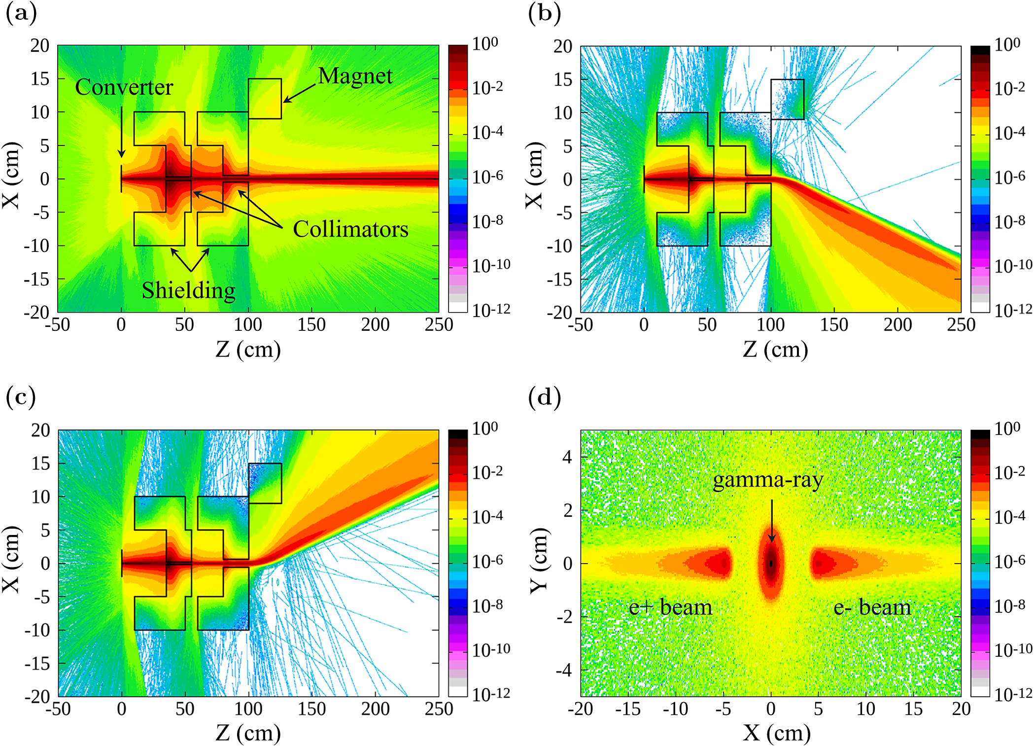
]. Lead shielding is added on both sides of the double collimators to shield off-axis noise. They must be placed axially symmetrically with the propagation axis of gamma rays. The lead shielding on both sides of the first collimator in Figure 1 is used to remove off-axis noise generated by the interaction of gamma rays with the converter. The collimated apertures are 5.5 and 10 mm, forming an acceptance angle of 10 mrad with the source. The lead shielding between the double collimators is used to shield the noise generated by the first collimator. The converter is set to a tungsten target, the collimator is set to lead material and the entire system is set in a vacuum, neglecting the effects of pair production interacting with air[
Reference Abramowicz, Almanza Soto, Altarelli, Aßmann, Athanassiadis, Avoni, Behnke, Benettoni, Benhammou, Bhatt, Blackburn, Blanch, Bonaldo, Boogert, Borysov, Borysova, Boudry, Breton, Brinkmann, Bruschi, Burkart, Büßer, Cavanagh, Dal Corso, Decking, Deniaud, Diner, Dosselli, Elad, Epshteyn, Esperante, Ferber, Firlej, Fiutowski, Fleck, Fuster-Martinez, Gadow, Gaede, Gallas, Garcia Cabrera, Gerstmayr, Ghenescu, Giorato, Golubeva, Grojean, Grutta, Grzelak, Hallford, Hartman, Heinemann, Heinzl, Helary, Hendriks, Hoffmann, Horn, Huang, Huang, Idzik, Irles, Jacobs, King, Klute, Kropf, Kroupp, Lahno, Lasagni Manghi, Lawhorn, Levanon, Levi, Levinson, Levy, Levy, Liberman, Liss, List, List, Lohmann, Maalmi, Madlener, Malka, Marsault, Mattiazzo, Meloni, Miron, Morandin, Moron, Nanni, Neagu, Negodin, Paccagnella, Pantano, Pietruch, Pomerantz, Pöschl, Potlog, Prasad, Quishpe, Ranken, Ringwald, Roich, Salgado, Santra, Sarri, Sävert, Sbrizzi, Schmitt, Schulthess, Schuwalow, Seipt, Simi, Soreq, Spataro, Streeter, Swientek, Tal Hod, Teter, Thiebault, Thoden, Trevisani, Urmanov, Vasiukov, Walker, Warren, Wing, Yap, Zadok, Zanetti, Zarnecki, Zbinkowski, Zembaczynski, Zepf, Zerwas, Ziegler and Zuffa
23
]. We set the thickness of the converter to 1 mm as previously optimized. The simulation includes the yoke of a C-shaped magnet that may be collided with low-energy electrons deflected by the magnetic field. The magnetic field is set to 1 tesla with a length of 32 cm (based on the actual magnet parameters). From Figures 3(a)–3(c) simulations demonstrate that after propagating through the spectrometer system, the distribution of electron–positron pairs at the detection plane exhibits a highly symmetric pattern, confirming effective collimation and a negligible off-axis noise contribution resulting from the optimized lead shielding geometry. In Figure 3(c), although electrons collide with the magnet yoke generating noise, their intensity has decayed by more than six orders of magnitude by the time when they reach the positron detection position, thus having no impact on the positron spectrum. Figure 3(d) shows the transverse distribution of electrons, positrons and photons at the back of the spectrometer. The detectors are symmetrically positioned along the dispersion axis in the deflection paths of electrons and positrons. As shown in the figure, the detectors exhibit a signal-to-noise ratio (SNR) of more than 10 dB, with signal intensities ranging from approximately
${10}^7$
photons propagating through the gamma-ray spectrometer simulated using the FLUKA code[
Reference Battistoni, Cerutti, Fassò, Ferrari, Muraro, Ranft, Roesler and Sala
36
]. Lead shielding is added on both sides of the double collimators to shield off-axis noise. They must be placed axially symmetrically with the propagation axis of gamma rays. The lead shielding on both sides of the first collimator in Figure 1 is used to remove off-axis noise generated by the interaction of gamma rays with the converter. The collimated apertures are 5.5 and 10 mm, forming an acceptance angle of 10 mrad with the source. The lead shielding between the double collimators is used to shield the noise generated by the first collimator. The converter is set to a tungsten target, the collimator is set to lead material and the entire system is set in a vacuum, neglecting the effects of pair production interacting with air[
Reference Abramowicz, Almanza Soto, Altarelli, Aßmann, Athanassiadis, Avoni, Behnke, Benettoni, Benhammou, Bhatt, Blackburn, Blanch, Bonaldo, Boogert, Borysov, Borysova, Boudry, Breton, Brinkmann, Bruschi, Burkart, Büßer, Cavanagh, Dal Corso, Decking, Deniaud, Diner, Dosselli, Elad, Epshteyn, Esperante, Ferber, Firlej, Fiutowski, Fleck, Fuster-Martinez, Gadow, Gaede, Gallas, Garcia Cabrera, Gerstmayr, Ghenescu, Giorato, Golubeva, Grojean, Grutta, Grzelak, Hallford, Hartman, Heinemann, Heinzl, Helary, Hendriks, Hoffmann, Horn, Huang, Huang, Idzik, Irles, Jacobs, King, Klute, Kropf, Kroupp, Lahno, Lasagni Manghi, Lawhorn, Levanon, Levi, Levinson, Levy, Levy, Liberman, Liss, List, List, Lohmann, Maalmi, Madlener, Malka, Marsault, Mattiazzo, Meloni, Miron, Morandin, Moron, Nanni, Neagu, Negodin, Paccagnella, Pantano, Pietruch, Pomerantz, Pöschl, Potlog, Prasad, Quishpe, Ranken, Ringwald, Roich, Salgado, Santra, Sarri, Sävert, Sbrizzi, Schmitt, Schulthess, Schuwalow, Seipt, Simi, Soreq, Spataro, Streeter, Swientek, Tal Hod, Teter, Thiebault, Thoden, Trevisani, Urmanov, Vasiukov, Walker, Warren, Wing, Yap, Zadok, Zanetti, Zarnecki, Zbinkowski, Zembaczynski, Zepf, Zerwas, Ziegler and Zuffa
23
]. We set the thickness of the converter to 1 mm as previously optimized. The simulation includes the yoke of a C-shaped magnet that may be collided with low-energy electrons deflected by the magnetic field. The magnetic field is set to 1 tesla with a length of 32 cm (based on the actual magnet parameters). From Figures 3(a)–3(c) simulations demonstrate that after propagating through the spectrometer system, the distribution of electron–positron pairs at the detection plane exhibits a highly symmetric pattern, confirming effective collimation and a negligible off-axis noise contribution resulting from the optimized lead shielding geometry. In Figure 3(c), although electrons collide with the magnet yoke generating noise, their intensity has decayed by more than six orders of magnitude by the time when they reach the positron detection position, thus having no impact on the positron spectrum. Figure 3(d) shows the transverse distribution of electrons, positrons and photons at the back of the spectrometer. The detectors are symmetrically positioned along the dispersion axis in the deflection paths of electrons and positrons. As shown in the figure, the detectors exhibit a signal-to-noise ratio (SNR) of more than 10 dB, with signal intensities ranging from approximately ${10}^{-4}$
to
${10}^{-4}$
to ${10}^{-2}$
particles/gamma photon per cm
${10}^{-2}$
particles/gamma photon per cm ${}^2$
.
${}^2$
.
Time-integrated fluence distribution for (a) photons, (b) positrons and (c) electrons resulting from the propagation of a monoenergetic gamma-ray beam. (d) The transverse distribution of electrons, positrons and photons at the back of the spectrometer. The color bar represents particles/gamma photons per square centimeter.

The energy resolution of a gamma-ray spectrometer is mainly limited by the resolution of the detector plane and the divergence of the incident particle beam[
Reference Cavanagh, Fleck, Streeter, Gerstmayr, Dickson, Ballage, Cadas, Calvin, Dufrénoy, Moulanier, Romagnani, Vasilovici, Whitehead, Specka, Cros and Sarri
22
, Reference Fleck
30
]. Taking factors such as the divergence angle $\Delta {\theta}_\mathrm{S}$
of the positrons/electrons after conversion, detector spatial resolution
$\Delta {\theta}_\mathrm{S}$
of the positrons/electrons after conversion, detector spatial resolution $\delta x$
(considering Fujifilm BAS-MS IP[
Reference Boutoux, Rabhi, Batani, Binet, Ducret, Jakubowska, Nègre, Reverdin and Thfoin
37
, Reference Bonnet, Comet, Denis-Petit, Gobet, Hannachi, Tarisien, Versteegen and Aléonard
38
]) and magnetic field inhomogeneity
$\delta x$
(considering Fujifilm BAS-MS IP[
Reference Boutoux, Rabhi, Batani, Binet, Ducret, Jakubowska, Nègre, Reverdin and Thfoin
37
, Reference Bonnet, Comet, Denis-Petit, Gobet, Hannachi, Tarisien, Versteegen and Aléonard
38
]) and magnetic field inhomogeneity $B(z)$
into account, the energy resolution is as follows:
$B(z)$
into account, the energy resolution is as follows:
 $$\begin{align}\frac{\delta E}{E}=\frac{E\left({L}_\mathrm{S}+{L}_\mathrm{M}+{L}_\mathrm{D}\right)\Delta {\theta}_\mathrm{S}\oplus E\delta x}{ce\int_0^{L_\mathrm{M}}B(z)\left({L}_\mathrm{M}-z+{L}_\mathrm{D}\right) \mathrm{d}z},\end{align}$$
where ${L}_\mathrm{M}$
is the length of the magnetic field,
${L}_\mathrm{M}$
is the length of the magnetic field, ${L}_\mathrm{S}$
is the distance between the converter and the magnet entrance,
${L}_\mathrm{S}$
is the distance between the converter and the magnet entrance, $c$
is the speed of light and
$c$
is the speed of light and ${L}_\mathrm{D}$
is the horizontal axial distance between the magnet exit and the detector. For our setup,
${L}_\mathrm{D}$
is the horizontal axial distance between the magnet exit and the detector. For our setup, ${L}_\mathrm{S}=1$
m,
${L}_\mathrm{S}=1$
m, ${L}_\mathrm{M}=32$
cm,
${L}_\mathrm{M}=32$
cm, ${L}_\mathrm{D}=70$
cm,
${L}_\mathrm{D}=70$
cm, $\Delta {\theta}_\mathrm{S}=10$
mrad,
$\Delta {\theta}_\mathrm{S}=10$
mrad, ${\delta x=25}$
μm and the magnetic field peak is 1.022 tesla. This could be expressed as
${\delta x=25}$
μm and the magnetic field peak is 1.022 tesla. This could be expressed as $\frac{\delta E}{E}$
= 0.24E[GeV]. For the 100 MeV particle,
$\frac{\delta E}{E}$
= 0.24E[GeV]. For the 100 MeV particle, $\delta E/E$
is calculated as 2.4%. Expanding the distance between the detector plane and the rear edge of the magnet (increasing
$\delta E/E$
is calculated as 2.4%. Expanding the distance between the detector plane and the rear edge of the magnet (increasing ${L}_\mathrm{D}$
), or increasing the longitudinal length of the shielding (assuming the aperture remains unchanged, reducing the divergence angle
${L}_\mathrm{D}$
), or increasing the longitudinal length of the shielding (assuming the aperture remains unchanged, reducing the divergence angle $\Delta {\theta}_\mathrm{S}$
), could significantly reduce this value. Note that our design is effective for gamma rays ranging from tens of MeV to a few GeV. For higher-energy gamma rays, the longitudinal size of the collimator and lead shielding needs to be increased.
$\Delta {\theta}_\mathrm{S}$
), could significantly reduce this value. Note that our design is effective for gamma rays ranging from tens of MeV to a few GeV. For higher-energy gamma rays, the longitudinal size of the collimator and lead shielding needs to be increased.
3 Learning procedure of gamma spectrum deconvolution
For specially designed gamma-ray spectrometers, the inverse solution algorithm for obtaining gamma-ray spectra needs to be specially devised. To describe the methodology for reconstructing the gamma-ray beam spectrum, let ${\mathcal{X}}_{\gamma}\left({E}_{\gamma}\right)$
be the energy distribution of the gamma rays, and
${\mathcal{X}}_{\gamma}\left({E}_{\gamma}\right)$
be the energy distribution of the gamma rays, and ${\mathcal{Y}}_l\left({E}_l\right)$
be the lepton pair (electron–positron pair) spectrum generated by gamma rays interacting with converters. This transformation process can be defined as follows:
${\mathcal{Y}}_l\left({E}_l\right)$
be the lepton pair (electron–positron pair) spectrum generated by gamma rays interacting with converters. This transformation process can be defined as follows:
 $$\begin{align}{\mathcal{Y}}_l\left({E}_l\right)=\int {\mathcal{X}}_{\gamma}\left({E}_{\gamma}\right){\mathcal{A}}_{\gamma l}\left({E}_{\gamma },{E}_l\right){\mathrm{d}E}_{\gamma },\end{align}$$
where ${\mathcal{A}}_{\gamma l}\left({E}_{\gamma },{E}_l\right)$
is the response matrix of the spectrometer system. Equation (3) is essentially a Fredholm integral equation of the first kind[
Reference Reginatto
39
], and solving the inverse problem belongs to the class of ill-posed problems. Using conventional methods to solve this inverse problem may result in a non-unique solution. Furthermore, slight noise introduced on the right-hand side of the equation may cause significant errors in the solution[
Reference Burova and Ryabov
40
]. We need to perform precise inversion of the photon spectrum under high-noise conditions. Since Poisson noise and Gaussian noise affect the measurement process, the inverse problem can be discretized into the following:
${\mathcal{A}}_{\gamma l}\left({E}_{\gamma },{E}_l\right)$
is the response matrix of the spectrometer system. Equation (3) is essentially a Fredholm integral equation of the first kind[
Reference Reginatto
39
], and solving the inverse problem belongs to the class of ill-posed problems. Using conventional methods to solve this inverse problem may result in a non-unique solution. Furthermore, slight noise introduced on the right-hand side of the equation may cause significant errors in the solution[
Reference Burova and Ryabov
40
]. We need to perform precise inversion of the photon spectrum under high-noise conditions. Since Poisson noise and Gaussian noise affect the measurement process, the inverse problem can be discretized into the following:
 $$\begin{align}{y}_i={A}_{ij}{x}_j+{\epsilon}_i.\end{align}$$
Here, the response matrix ${A}_{ij}$
and the statistical noise
${A}_{ij}$
and the statistical noise ${\epsilon}_i$
, mainly from Poisson and Gaussian counts, are separated[
Reference Zhang, Zhu and Bao
41
]. The advantage of this approach is to simulate the response matrix using the Geant4 MC code by considering the geometric structure of the gamma-ray spectrometer and the experimental environment. The problem can then be decomposed into two steps: denoising and reconstruction.
${\epsilon}_i$
, mainly from Poisson and Gaussian counts, are separated[
Reference Zhang, Zhu and Bao
41
]. The advantage of this approach is to simulate the response matrix using the Geant4 MC code by considering the geometric structure of the gamma-ray spectrometer and the experimental environment. The problem can then be decomposed into two steps: denoising and reconstruction.
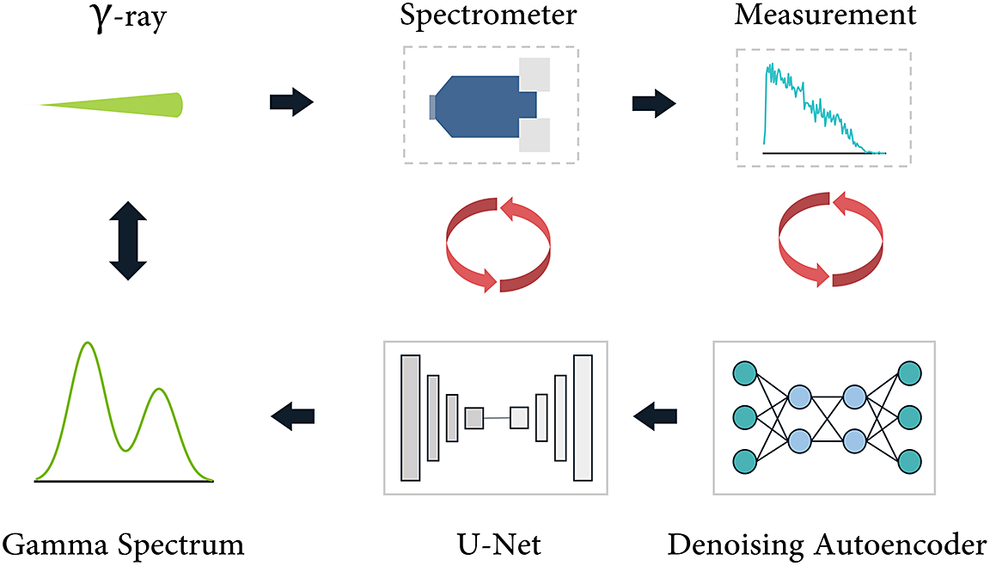
The overall reconstruction workflow, depicted in Figure 4, is organized into two sequential stages: denoising and deconvolution. In the denoising stage, we assemble a comprehensive training set composed chiefly of MC-simulated spectra supplemented by a subset of experimentally acquired data from the experimental data. This hybrid dataset is used to train a supervised DAE, which learns to suppress measurement noise while preserving key spectral features. In the subsequent deconvolution stage, the trained network replaces conventional iterative solvers, such as the simultaneous iterative reconstruction technique (SIRT)[ Reference Haden, Golovin, Yan, Fruhling, Zhang, Zhao, Banerjee and Umstadter 18 ] or the expectation maximization method (e.g., Richardson–Lucy algorithm[ Reference Li, Li, Lv, Duan, Haerken and Zhao 42 ]) by performing paired-spectrum inversion in a single forward pass. Here, we employ a U-Net architecture, carefully tuning hyperparameters to optimize convergence and generalization. Below, we detail the procedure for generating synthetic spectra and characterizing the detector response matrix, the design and configuration of the U-Net model and the training regimen used to achieve robust, high-fidelity spectrum reconstruction.
Schematic of the overall reconstruction workflow, organized into two sequential stages: (1) denoising – a supervised autoencoder is trained on a hybrid dataset to suppress measurement noise while retaining key spectral features; (2) deconvolution – the trained network, built on a U-Net architecture. This figure can be viewed as illustrating the forward and inverse processes of Equation (4).

3.1 Dataset generation
A comprehensive gamma-ray energy spectrum dataset is generated by combining over 30 different base spectra, typical radiation spectra and experimental data from various sources (0.01–1 GeV). The base spectra include Gaussian distributions, exponential decay functions, step functions and arbitrary random distributions across bins. Typical radiation spectra consist of monoenergetic spectra, bremsstrahlung spectra, synchrotron-like radiation spectra and inverse Compton scattering spectra. Experimental data are derived from bremsstrahlung and inverse Compton scattering spectra generated in the experiments conducted at the Key Laboratory for Laser Plasmas (LLP) at Shanghai Jiao Tong University (SJTU)[ Reference Chen, Yan, Zhu, Li, Hu, Xu, Zhou, Lu, Wei, Lu, Ge, Li, Yuan, Liu, Chen, Chen and Zhang 43 , Reference Li, Chen, Chen, Liu, Gu, Guo, Hua, Huang, Leng, Li, Li, Li, Lin, Lu, Lyu, Ma, Ning, Peng, Wan, Wang, Wang, Wei, Yan, Zhang, Zhao, Zhao, Zhou, Zhou, Zhou, Zhu and Zhu 44 ].
The parameters of the positron energy spectrum (e.g., peak position, width, intensity) obtained by convolving the photon spectrum with the response matrix $\mathcal{A}$
described in Section 3.2 are randomly sampled from a physically relevant range. To enhance the applicability of the data, data augmentation techniques are applied, including noise injection, random superposition and spectrum-type manipulation. Gaussian–Poisson mixed noise with random amplitudes ranging from 0% to 10% (based on the worst-case SNR of the spectrometer) is added to the spectra. Multiple spectra are linearly superimposed to form new spectra, generating realistic radiation patterns observed in experiments (e.g., double-peak or multi-peak structures)[
Reference Angioi, Mackenroth and Di Piazza
45
, Reference Heinzl, King and MacLeod
46
]. Spectrum-type manipulation involves random scaling, shifting and the injection of additional peaks.
$\mathcal{A}$
described in Section 3.2 are randomly sampled from a physically relevant range. To enhance the applicability of the data, data augmentation techniques are applied, including noise injection, random superposition and spectrum-type manipulation. Gaussian–Poisson mixed noise with random amplitudes ranging from 0% to 10% (based on the worst-case SNR of the spectrometer) is added to the spectra. Multiple spectra are linearly superimposed to form new spectra, generating realistic radiation patterns observed in experiments (e.g., double-peak or multi-peak structures)[
Reference Angioi, Mackenroth and Di Piazza
45
, Reference Heinzl, King and MacLeod
46
]. Spectrum-type manipulation involves random scaling, shifting and the injection of additional peaks.
Two priors are specifically considered: pair production must exceed 1.022 MeV, and the spectrum must remain non-negative. The augmented spectra are normalized in terms of photon number and subjected to non-negativity constraints. The final dataset consists of the original spectra $X$
and the noisy measurements
$X$
and the noisy measurements $Y$
obtained after convolution with the detector response. Details on constructing the response matrix
$Y$
obtained after convolution with the detector response. Details on constructing the response matrix $\mathcal{A}$
can be found in Section 3.2.
$\mathcal{A}$
can be found in Section 3.2.
3.2 Building response matrix $\mathcal{A}$

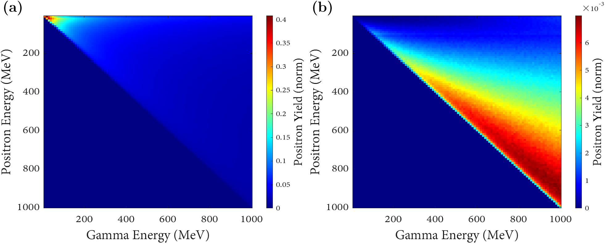
The gamma-ray spectrometer shown in Figure 3 is reproduced in a Geant4 MC simulation. This model integrates precise detector geometry (including the magnet spectrometer section and the effect of air) and relevant physical processes (the photoelectric effect, Compton scattering and pair production) to characterize its response capabilities realistically.
A series of monoenergetic gamma-ray sources, spanning the desired energy range, is simulated to interact with the system. We collect positron signals by placing detectors behind the converter and behind the magnet, respectively. For each energy, we count the detected positron energies across the corresponding detector channels, thereby populating columns of the discrete response matrix ${A}_{ij}$
. The simulated response matrix
${A}_{ij}$
. The simulated response matrix $\mathcal{A}$
, shown in Figure 5, consists of two panels that respectively illustrate the responses of the converter and the energy spectrometer system to monoenergetic gamma rays. The heatmaps present the received energy on the detector plane versus the incident gamma-ray energy, highlighting how the system responds to various gamma-ray energies. In the discrete representation
$\mathcal{A}$
, shown in Figure 5, consists of two panels that respectively illustrate the responses of the converter and the energy spectrometer system to monoenergetic gamma rays. The heatmaps present the received energy on the detector plane versus the incident gamma-ray energy, highlighting how the system responds to various gamma-ray energies. In the discrete representation ${A}_{ij}$
, each column
${A}_{ij}$
, each column $j$
encodes the probability distribution of positron energies
$j$
encodes the probability distribution of positron energies $\left\{{E}_l^i\right\}$
arising from a monoenergetic gamma-ray with energy
$\left\{{E}_l^i\right\}$
arising from a monoenergetic gamma-ray with energy ${E}_{\gamma}^j$
. This results in moving from a specialized Fredholm-type equation to a Volterra integral equation of the first kind , which has a variable limit of integration. This has advantages and disadvantages for the framing of the inverse problem. The upper-triangular nature of the heatmaps is indicative of the causal constraint, where non-zero entries appear only when the incident photon energy exceeds the positron energy.
${E}_{\gamma}^j$
. This results in moving from a specialized Fredholm-type equation to a Volterra integral equation of the first kind , which has a variable limit of integration. This has advantages and disadvantages for the framing of the inverse problem. The upper-triangular nature of the heatmaps is indicative of the causal constraint, where non-zero entries appear only when the incident photon energy exceeds the positron energy.
Multiple response functions were generated by simulating the monoenergetic gamma-ray response using different systems within the Geant4 framework. Vertical lineouts of this figure show the positron spectrum generated at a specific gamma-ray energy. (a) Ideal converter response of monoenergetic gamma rays interacting with a 1 mm tungsten converter. (b) Response function of a gamma-ray spectrometer configured as shown in Figure 1 with a 1 mm tungsten converter.

The transition from Figure 5(a) to Figure 5(b) shows a sharp decay in the singular-value spectrum of $\mathcal{A}$
, producing an exceedingly larger condition number. Inversion by the least squares method therefore amplifies any measurement noise – whether Poisson or Gaussian – in the small singular-value modes, producing non-physical oscillations or negative features in the recovered spectrum.
$\mathcal{A}$
, producing an exceedingly larger condition number. Inversion by the least squares method therefore amplifies any measurement noise – whether Poisson or Gaussian – in the small singular-value modes, producing non-physical oscillations or negative features in the recovered spectrum.
The ill-conditioning of the response matrix, characterized by a rapidly decaying singular-value spectrum and minimal channel overlap[ Reference Hansen 47 ], means that any conventional inverse solver – even with standard Tikhonov or truncated singular-value decomposition (SVD) regularization – inevitably sacrifices either resolution or stability. Moreover, the photon counting statistics introduce heteroscedastic noise that cannot be uniformly damped by a single global regularization parameter. These limitations motivate the adoption of a data-driven inversion strategy.
3.3 Denoising autoencoder: spectral feature extractor
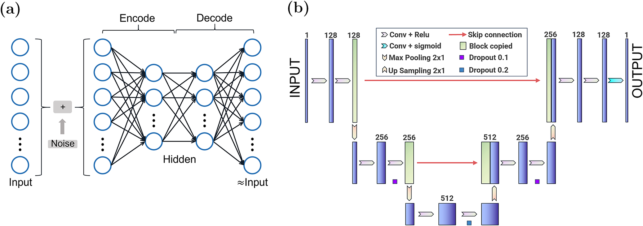
To extract the ‘pure physical signal’ from the ‘contaminated’ positron spectrum, we introduce a supervised DAE that distinguishes the underlying physical positron distribution from background interference. DAEs have already been used as a preprocessing technique for specific spectrometer systems[ Reference Zhang, Zhu and Bao 41 ], where the original measurement data are denoised before reconstruction, and then the spectrum is reconstructed based on the denoised data. Figure 6(a) presents a schematic of the DAE architecture, highlighting its encoder–decoder symmetry structure optimized for one-dimensional (1D) spectral data.
-
• Encoder: the positron energy spectrum input undergoes two stages of nonlinear transformation, progressively compressing its data dimensions. This process essentially extracts key physical features determining the spectral shape from noisy measurement signals while filtering out random statistical noise.
-
• Decoder: based on extracted core features, the synthesized signal is restored to a positron spectrum signal matching the input length through a reverse nonlinear transformation. The final output is a high-fidelity spectrum that maximally suppresses random fluctuations on the original spectra.
Training is performed on 500,000 paired spectra (see, in Section 3.1) containing ${X}_{\mathrm{clean}},{Y}_{\mathrm{noisy}}$
, where
${X}_{\mathrm{clean}},{Y}_{\mathrm{noisy}}$
, where ${X}_{\mathrm{clean}}$
spans analytic base shapes, MC-simulated mixtures and a subset of experimental measurements, and
${X}_{\mathrm{clean}}$
spans analytic base shapes, MC-simulated mixtures and a subset of experimental measurements, and ${Y}_{\mathrm{noisy}}=A\kern0.1em {X}_{\mathrm{clean}}+\epsilon$
incorporates both Poisson and Gaussian perturbations at amplitudes up to 10%. We optimize the mean-squared error (MSE) between the autoencoder output and
${Y}_{\mathrm{noisy}}=A\kern0.1em {X}_{\mathrm{clean}}+\epsilon$
incorporates both Poisson and Gaussian perturbations at amplitudes up to 10%. We optimize the mean-squared error (MSE) between the autoencoder output and ${Y}_{\mathrm{clean}}$
using the Adam optimizer (learning rate
${Y}_{\mathrm{clean}}$
using the Adam optimizer (learning rate ${10}^{-3}$
). During each epoch, fresh noise realizations and random amplitude augmentations ensure robust generalization across count rates and spectral shapes.
${10}^{-3}$
). During each epoch, fresh noise realizations and random amplitude augmentations ensure robust generalization across count rates and spectral shapes.
Schematic of machine learning architecture. (a) Denoising autoencoder (DAE) with symmetric encoder–decoder structure for suppressing statistical noise in measured positron spectra. The DAE acts as a spectral feature extractor to separate the physical positron energy distribution from stochastic noise components such as counting fluctuations and stray electron backgrounds. The input is the noisy positron energy spectrum and the output is the denoised positron energy spectrum. (b) U-Net functions as a nonlinear deconvolution operator with an encoder–decoder structure and skip connections to solve inverse problems, reconstructing incident gamma-ray spectra from denoised positron energy spectra. The input is the denoised positron energy spectrum and the output is the deconvolved gamma-ray energy spectrum.

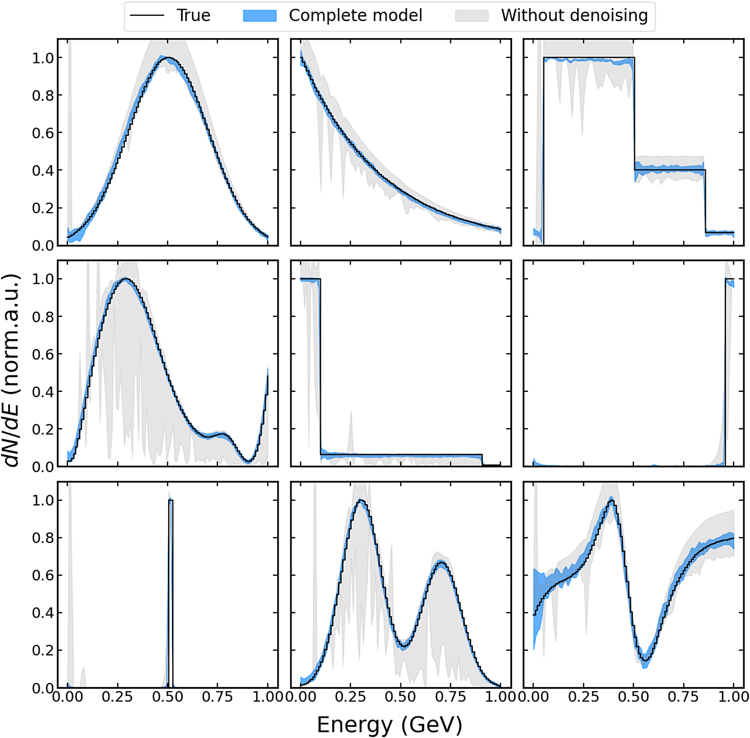
On a held-out test set of 50,000 spectra, the DAE achieves an average SNR of 30.2 dB and a mean absolute error below 10% compared to the directly deconvolved data without denoising. As can be seen, the role of the DAE is indispensable in high-noise conditions (see Figure 7). By suppressing stochastic noise to levels suitable for downstream inversion and quantitative analysis, we substantially improve the stability and resolution of the subsequent U-Net-based inversion.
The reconstructed photon spectrum obtained by applying machine learning algorithms to the dataset (for the convenience of presentation, all the data have been normalized to the maximum value). The black line shows the photon spectrum incident on the spectrometer in the simulation. The blue shaded band indicates the 95% Bayesian credible interval (Monte Carlo uncertainty) calculated by the algorithm. The shaded gray represents the result of deconvolution without denoising.

3.4 U-Net: nonlinear deconvolution operator
To address the ill-posed nature of the inverse problem in gamma-ray spectrum reconstruction, we employ a U-Net architecture, which is well-suited for deconvolution tasks, particularly in the presence of noise. The U-Net is a convolutional neural network[ Reference Hu, Hu, Gong and Si 48 ], and it is adapted as a nonlinear deconvolution operator to map the measured positron distribution back to the incident gamma-ray energy spectrum[ Reference Döpp, Eberle, Howard, Irshad, Lin and Streeter 49 ]. The U-Net architecture consists of an encoder–decoder structure with skip connections, which facilitates the preservation of fine spectral features during the reconstruction process[ Reference Ronneberger, Fischer, Brox, Navab, Hornegger, Wells and Frangi 50 ].
This network is summarized in Figure 6(b). The encoder starts with a 1D convolutional layer, followed by rectified linear unit (ReLU) activations to introduce the nonlinear transformation and max-pooling operations to preserve the most significant spectral line features. These layers progressively reduce the dimensionality of the input positron spectra while learning to capture the spectral shape and intensity distribution. The bottleneck layer captures the most essential physical representation, forming the core energy-intensity distribution necessary for stable inversion in ill-posed conditions. The decoder progressively reconverts the extracted core physical features back into a high-resolution energy spectrum distribution, thereby enabling the reconstruction of the spectra. Skip connections function as an information bridge for fine-structure preservation. They ensure that high-resolution spectral details (such as narrow peaks), which may be smoothed during global feature extraction, are directly reintegrated into the final reconstruction, maintaining the spectral fidelity. The final output layer produces the reconstructed gamma-ray spectrum, ensuring that it satisfies the physical constraints, such as non-negativity.
The U-Net was implemented using a Keras framework with a TensorFlow backend[ Reference Abadi, Agarwal, Barham, Brevdo, Chen, Citro, Corrado, Davis, Dean, Devin, Ghemawat, Goodfellow, Harp, Irving, Isard, Jia, Jozefowicz, Kaiser, Kudlur, Levenberg, Mane, Monga, Moore, Murray, Olah, Schuster, Shlens, Steiner, Sutskever, Talwar, Tucker, Vanhoucke, Vasudevan, Viegas, Vinyals, Warden, Wattenberg, Wicke, Yu and Zheng 51 ], and the model is trained to minimize the MSE between the reconstructed spectrum and the true spectrum. The loss function used is as follows:
 $$\begin{align}\mathrm{\mathcal{L}}\left(\theta \right)=\frac{1}{N}\sum \limits_{i=1}^N{\left({\mathcal{Y}}_i-{\widehat{\mathcal{Y}}}_i\right)}^2,\end{align}$$
where ${\mathcal{Y}}_i$
represents the true clean spectrum,
${\mathcal{Y}}_i$
represents the true clean spectrum, ${\widehat{\mathcal{Y}}}_i$
is the predicted spectrum and
${\widehat{\mathcal{Y}}}_i$
is the predicted spectrum and $N$
is the total number of samples in the batch. The model is trained using the Adam optimizer with a learning rate of
$N$
is the total number of samples in the batch. The model is trained using the Adam optimizer with a learning rate of ${10}^{-3}$
[
Reference Kingma and Ba
52
], which balances convergence efficiency and prevents overfitting to noise.
${10}^{-3}$
[
Reference Kingma and Ba
52
], which balances convergence efficiency and prevents overfitting to noise.
The structural parameters (hyperparameters) are optimized to match the spectrometer’s physical characteristics. We use large kernel sizes (set to nine or seven) to capture the overall shape of the positron energy spectrum distribution, helping the network ignore local statistical fluctuations. The initial layers use 128 channels with a convolution width corresponding to approximately 100 energy units, using a kernel size of nine. As the network goes deeper, the channel count increases to 512 while the convolution width narrows to 25 units, allowing the model to focus on core spectral components. Dropout regularization is applied to stabilize training and enhance the model’s generalization across different spectra.
Training is performed on the dataset mentioned in Section 3.1. The final dataset consists of 500,000 pairs of clean and noisy spectra, used for training the network. To restore the original scale of the reconstructed gamma spectrum, it is crucial to address the relationship between the photon spectrum and its integral normalization. The photon spectrum is essentially the product of the photon count and the normalized differential energy spectrum $\frac{\mathrm{d}N}{\mathrm{d}E}$
. In this framework, the U-Net model learns the mapping between the normalized outputs
$\frac{\mathrm{d}N}{\mathrm{d}E}$
. In this framework, the U-Net model learns the mapping between the normalized outputs $Y$
and
$Y$
and $X$
. The activation function of the output layer is sigmoid, which maps
$X$
. The activation function of the output layer is sigmoid, which maps $X$
into the range
$X$
into the range $\left[0,1\right]$
. To recover the original energy spectrum, the output of the model must be subjected to a final integral normalization. Experimentally, the original gamma photon spectrum can be derived by using the photon counts from imaging plates and the normalized energy spectrum obtained through simulations.
$\left[0,1\right]$
. To recover the original energy spectrum, the output of the model must be subjected to a final integral normalization. Experimentally, the original gamma photon spectrum can be derived by using the photon counts from imaging plates and the normalized energy spectrum obtained through simulations.
4 Evaluation results
The results of the deconvolution process are shown in Figure 7, where nine representative spectra with different parameters from the database were used to test the trained model. The black line is the original gamma-ray spectrum, the shaded gray represents the result of deconvolution without denoising and the light blue confidence band represents model uncertainty. This figure also illustrates that the denoising process and the deconvolution process are closely related. Under high-noise conditions, the deconvolution process fails to accurately capture certain features of the original spectrum, and the impact of Poisson noise is significant. The uncertainty is employed as a measure of the model’s confidence in its predicted values, quantified through MC dropout sampling. This process can be understood through the equivalence between dropout training and variational inference[
Reference Gal and Ghahramani
53
], where dropout acts as a regularization technique and is equivalent to Bayesian inference of the weight distribution. During spectrum reconstruction ${y}^{\ast}\to {x}^{\ast }$
, we sample
${y}^{\ast}\to {x}^{\ast }$
, we sample $T$
weight configurations via dropout as follows[
Reference Gal and Ghahramani
53
]:
$T$
weight configurations via dropout as follows[
Reference Gal and Ghahramani
53
]:
 $$\begin{align}\mathbb{E}\left[{x}^{\ast}\right]\approx \frac{1}{T}\sum \limits_{t=1}^T{f}^{W_t}\left({y}^{\ast}\right),\quad {W}_t\sim q\theta (W),\end{align}$$
where ${y}^{\ast }$
is the input lepton spectrum,
${y}^{\ast }$
is the input lepton spectrum, ${x}^{\ast }$
is the reconstructed spectrum and
${x}^{\ast }$
is the reconstructed spectrum and $\mathbb{E}\left[{x}^{\ast}\right]$
represents the expected reconstruction computed by averaging over multiple weight configurations
$\mathbb{E}\left[{x}^{\ast}\right]$
represents the expected reconstruction computed by averaging over multiple weight configurations ${W}_t$
sampled from the Bayesian distribution
${W}_t$
sampled from the Bayesian distribution $q\theta (W)$
. It is viable to calculate the model’s predictive variance:
$q\theta (W)$
. It is viable to calculate the model’s predictive variance:
 $$\begin{align}\sigma =\sqrt{\frac{1}{T}\sum \limits_{t=1}^T{\left({f}^{W_t}\left({y}^{\ast}\right)-\mathbb{E}\left[{x}^{\ast}\right]\right)}^2}.\end{align}$$
Although not shown, the reconstruction of the electron spectrum produces similar results and can be used as a consistency check[ Reference Cavanagh, Fleck, Streeter, Gerstmayr, Dickson, Ballage, Cadas, Calvin, Dufrénoy, Moulanier, Romagnani, Vasilovici, Whitehead, Specka, Cros and Sarri 22 ]. The spectral shape of the incident photon spectrum is well reconstructed within the 95% Bayesian credible interval (BCI) of the reconstruction results.
The 95% BCI presented in this work is quantitatively defined as follows. For each energy channel $i$
of the reconstructed spectrum, we compute the posterior distribution of the predicted flux value,
$i$
of the reconstructed spectrum, we compute the posterior distribution of the predicted flux value, $p\left({x}_i^{\ast }|{y}^{\ast}\right)$
, based on
$p\left({x}_i^{\ast }|{y}^{\ast}\right)$
, based on $T$
stochastic forward passes using MC dropout. The 95% BCI for channel
$T$
stochastic forward passes using MC dropout. The 95% BCI for channel $i$
is then defined as the equal-tailed interval bounded by the
$i$
is then defined as the equal-tailed interval bounded by the $2.5$
and
$2.5$
and $97.5$
percentiles of this empirical posterior distribution. Mathematically, the interval
$97.5$
percentiles of this empirical posterior distribution. Mathematically, the interval $\left[{L}_i,{U}_i\right]$
satisfies the following:
$\left[{L}_i,{U}_i\right]$
satisfies the following:
 $$\begin{align}P\left({L}_i\le {x}_i^{\ast}\le {U}_i|{y}^{\ast}\right)=0.95,\end{align}$$
where ${L}_i$
and
${L}_i$
and ${U}_i$
are the lower and upper bounds of the credible interval for the
${U}_i$
are the lower and upper bounds of the credible interval for the $i$
th energy channel, respectively. This implies that, given the observed lepton spectrum
$i$
th energy channel, respectively. This implies that, given the observed lepton spectrum ${y}^{\ast }$
, there is a 95% probability that the true value of the incident photon flux in channel
${y}^{\ast }$
, there is a 95% probability that the true value of the incident photon flux in channel $i$
lies within the interval
$i$
lies within the interval $\left[{L}_i,{U}_i\right]$
. The light blue confidence band in Figure 7 is generated by connecting the
$\left[{L}_i,{U}_i\right]$
. The light blue confidence band in Figure 7 is generated by connecting the ${L}_i$
and
${L}_i$
and ${U}_i$
values across all energy channels, providing a visual representation of the model’s uncertainty over the entire reconstructed spectrum.
${U}_i$
values across all energy channels, providing a visual representation of the model’s uncertainty over the entire reconstructed spectrum.
The performance of gamma-ray energy spectrum reconstruction is evaluated using three metrics: the root mean square error (RMSE), peak signal-to-noise ratio (PSNR) and structural similarity (SSIM)[ Reference Mostafapour, Gholamiankhah, Dadgar, Arabi and Zaidi 54 ]. The RMSE is a classic statistical measure of the average deviation between the reconstructed spectrum and the reference spectrum. It is defined as the square root of the mean of the sum of the squares of the errors in all energy channels:
 $$\begin{align}\mathrm{RMSE}=\sqrt{\frac{1}{N}\sum \limits_{i=1}^N{\left({\hat{x}}_i-{x}_i\right)}^2},\end{align}$$
where ${x}_i$
and
${x}_i$
and ${\hat{x}}_i$
represent the true count and reconstructed count for the
${\hat{x}}_i$
represent the true count and reconstructed count for the $i$
th channel, respectively, and
$i$
th channel, respectively, and $N$
is the total number of channels. The RMSE is sensitive to large deviations and increases significantly when the reconstruction overestimates or underestimates the counts in certain energy channels, thereby reflecting the overall reconstruction accuracy at a rough level. The PSNR originates from the field of image processing and is used to measure the contrast strength between signals and noise on two spectral lines. Its formula is typically written as follows:
$N$
is the total number of channels. The RMSE is sensitive to large deviations and increases significantly when the reconstruction overestimates or underestimates the counts in certain energy channels, thereby reflecting the overall reconstruction accuracy at a rough level. The PSNR originates from the field of image processing and is used to measure the contrast strength between signals and noise on two spectral lines. Its formula is typically written as follows:
 $$\begin{align}\mathrm{PSNR}=10{\log}_{10}\left(\frac{{\operatorname{MAX}}^2}{\mathrm{MSE}}\right),\end{align}$$
where $\operatorname{MAX}$
is the maximum count value of the true spectral line and
$\operatorname{MAX}$
is the maximum count value of the true spectral line and $\mathrm{MSE}$
is the square of the aforementioned RMSE. The PSNR is measured in decibels (dB), with higher values indicating that the reconstructed spectral line retains more of the original signal features overall, and the relative contribution of noise and reconstruction error is reduced. SSIM focuses on preserving the local structure and contrast details of the spectral line. Its core idea is that a high-similarity reconstruction should not only be close in amplitude but also consistent in shape and contrast. For spectral line segment
$\mathrm{MSE}$
is the square of the aforementioned RMSE. The PSNR is measured in decibels (dB), with higher values indicating that the reconstructed spectral line retains more of the original signal features overall, and the relative contribution of noise and reconstruction error is reduced. SSIM focuses on preserving the local structure and contrast details of the spectral line. Its core idea is that a high-similarity reconstruction should not only be close in amplitude but also consistent in shape and contrast. For spectral line segment $x$
and reconstructed segment
$x$
and reconstructed segment $y$
, SSIM is typically defined as follows:
$y$
, SSIM is typically defined as follows:
 $$\begin{align}\mathrm{SSIM}\left(x,y\right)=\frac{\left(2{\mu}_x{\mu}_y+{C}_1\right)\left(2{\sigma}_{xy}+{C}_2\right)}{\left({\mu}_x^2+{\mu}_y^2+{C}_1\right)\left({\sigma}_x^2+{\sigma}_y^2+{C}_2\right)},\end{align}$$
where $\mu$
and
$\mu$
and $\sigma$
denote the local mean and variance, respectively, and
$\sigma$
denote the local mean and variance, respectively, and ${\sigma}_{xy}$
is the covariance. The constants
${\sigma}_{xy}$
is the covariance. The constants ${{C}_1={\left({k}_1L\right)}^2}$
,
${{C}_1={\left({k}_1L\right)}^2}$
, ${C}_2={\left({k}_2L\right)}^2$
are small constants used to stabilize the denominator, where L is the dynamic range of the spectral values (i.e., the maximum value minus the minimum value), typically taken as
${C}_2={\left({k}_2L\right)}^2$
are small constants used to stabilize the denominator, where L is the dynamic range of the spectral values (i.e., the maximum value minus the minimum value), typically taken as ${k}_1=0.01$
,
${k}_1=0.01$
, ${k}_2=0.03$
. The SSIM value is in the range of
${k}_2=0.03$
. The SSIM value is in the range of $\left[0,1\right]$
. The closer it is to 1, the more consistent the reconstructed spectral line is with the reference spectral line in terms of detail and overall structure.
$\left[0,1\right]$
. The closer it is to 1, the more consistent the reconstructed spectral line is with the reference spectral line in terms of detail and overall structure.
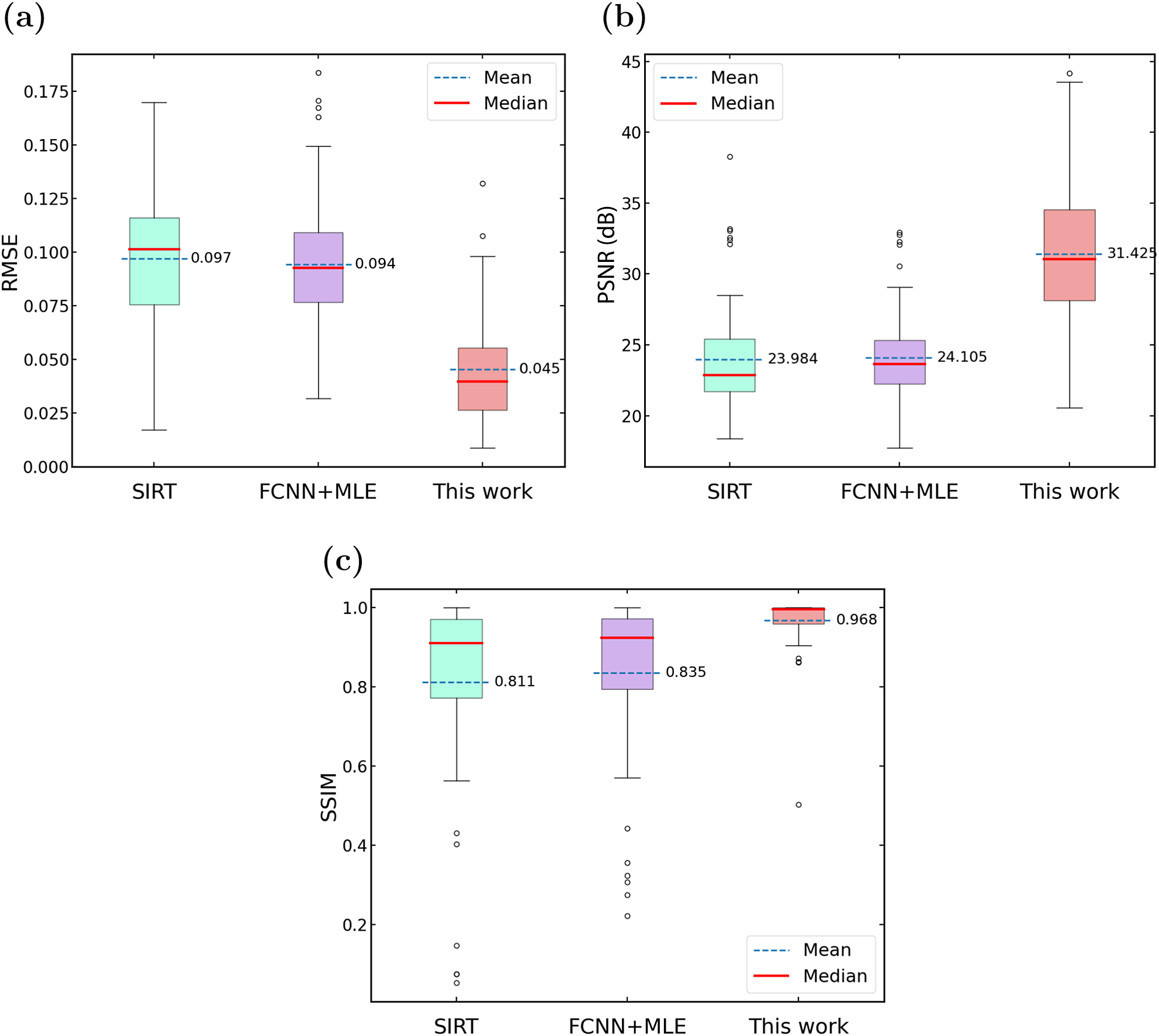
To demonstrate performance, we reproduced the configurations of the SIRT and the hybrid approach using fully connected neural networks to generate an informed initial guess for iterative MLE[ Reference Haden, Golovin, Yan, Fruhling, Zhang, Zhao, Banerjee and Umstadter 18 , Reference Yadav, Oruganti, Naranjo, Andonian, Apsimon, Welsch and Rosenzweig 29 ]. The statistical results of 300 test datasets (average SNR approximately 35.70 dB) evaluated using three methods are shown in Figure 8. Clearly, our method achieved the lowest RMSE and the highest PSNR and SSIM in the comparison.
Performance of different models: (a) RMSE; (b) PSNR; (c) SSIM for the SIRT algorithm, FCNN+MLE model and our deep learning approach. The boxplots demonstrate the distribution of each metric over 300 test spectra. For the RMSE, lower values indicate better performance, while for the PSNR and SSIM, higher values are desirable. The red line represents the median value. The blue dashed line represents the average value of the data. FCNN, fully connected neural network.

5 Conclusion and outlook
In this study, we have developed an approach for high-fidelity gamma-ray spectroscopy in the multi-MeV to GeV range, enabling the reconstruction of photon energy spectra under high-noise conditions through the integration of optimized spectrometer parameters and the machine learning deconvolution algorithm. It should be stressed that this type of spectrometer is almost transparent to the gamma rays, with only a small percentage of them interacting. It can thus be used in conjunction with other gamma-ray detectors (profilers and polarimeters). We propose a machine learning framework, which combines a DAE for statistical-noise suppression with a U-Net architecture for spectral deconvolution. DAEs, trained specifically to remove 90% or more of the input noise, function analogously to a smoothing operation. Also, U-Net architectures demonstrate robustness, effectively reconstructing the original energy spectrum from partially noisy data. This approach effectively solves the ill-posed inverse problem inherent in gamma-ray spectroscopy, overcoming limitations of traditional algorithms such as the SIRT and hybrid methods.
Validation against a diverse dataset of synthetic and experimental spectra performs well, with our method achieving the lowest RMSE and highest PSNR and SSIM among compared techniques. The machine learning architecture’s ability to preserve spectral features while suppressing noise enables robust reconstruction of complex spectral shapes, including those with multi-peak structure characteristic of nonlinear Compton scattering and LWFA-driven bremsstrahlung.
The present spectrometer is designed to operate robustly for photon energies of more than approximately 50 MeV up to the order of a few GeV. In future strong-field laser physics experiments, extending the energy range to several GeV or more would require enlarging spectrometer components and optimizing noise shielding to account for higher-order quantum electrodynamics (QED) processes. Further work will cover multi-parameter reconstruction (e.g., the angular distribution of incident photons). The ability to extract the ‘double-differential’ of the photon beam (i.e., $\frac{\mathrm{d}^2N}{\mathrm{d}E\mathrm{d}\theta}$
) would be great for SFQED experiments. This work establishes a foundation for next-generation gamma-ray diagnostics, with implications for fundamental SFQED studies, laboratory astrophysics and compact radiation sources.
$\frac{\mathrm{d}^2N}{\mathrm{d}E\mathrm{d}\theta}$
) would be great for SFQED experiments. This work establishes a foundation for next-generation gamma-ray diagnostics, with implications for fundamental SFQED studies, laboratory astrophysics and compact radiation sources.
Acknowledgements
This work was supported by the National Key Research and Development Program of China (Grant No. 2021YFA1601700), the AI for Science Program, Shanghai Municipal Commission of Economy and Informatization (Grand No. 2025-GZL-RGZN-BTBX-02029), the Fundamental and Interdisciplinary Disciplines Breakthrough Plan of the Ministry of Education of China (Grant No. JYB2025XDXM204), the National Natural Science Foundation of China (Grant Nos. 12074251, 11991073 and 12175140) and the Engineering and Physical Sciences Research Council (EPSRC) (Grant EP/V049186/1). The authors would like to acknowledge the sponsorship from the Yangyang Development Fund. The computations in this paper were run on the Siyuan-1 cluster supported by the Center for High Performance Computing at Shanghai Jiao Tong University.


 Open access

