Introduction

Ice losses by calving exceed ablation by surface melting on the Antarctic and Greenland ice sheets, and calving is a significant ablation process on many other high- and mid-latitude ice masses. Because calving fluxes are strongly influenced by ice velocities, dynamic changes to outlet glaciers and ice streams can have a large effect on ice-sheet mass balance, providing a mechanism for rapid transfer of water to the oceans. Recently, calving glaciers in many parts of the world have undergone dramatic acceleration and retreat (e.g. Reference VenterisVenteris, 1999; Reference Thomas, Rignot, Kanagaratnam, Krabill and CasassaThomas and others, 2004; Reference Howat, Joughin, Tulaczyk and GogineniHowat and others, 2005; Reference Luckman and MurrayLuckman and Murray, 2005; Reference Rignot and KanagaratnamRignot and Kanagaratnam, 2006), indicating a highly nonlinear response to initial climatic forcing. Despite their important role in modulating the effects of climate change, the dynamics of calving glaciers are very poorly represented in existing ice-sheet models and constitute the largest source of uncertainty in predictions of future ice-sheet evolution. Development of a comprehensive general model of calving glacier dynamics is a formidable challenge involving some of the most stubborn problems in glaciology, including realistic parameterization of calving processes, the ‘grounding-line problem’ (e.g. Reference Vieli and PayneVieli and Payne, 2005) and the ‘unresolved sliding problem’ (Reference WeertmanWeertman, 1979). In this paper, we present a new framework for modelling tidewater glacier dynamics, using a new physically based calving criterion and alternative sliding functions. (Although not ‘laws’ in the physical sense, calving criteria and sliding functions are often referred to as such in the literature, and for convenience this convention is followed here.) Specifically we (1) assess the role of strain rates in calving processes and calving glacier dynamics, (2) explore feedback processes between strain rates, thinning, flow acceleration and terminus retreat, and (3) show how the new framework can be used to represent a wide range of behaviours observed in tidewater glaciers and ice streams.

‘Calving Laws’

Calving rate, U _C, is defined as the difference between ice velocity at the glacier terminus and glacier length change over time:

where ŪT is the depth-averaged velocity at the glacier terminus, L is the glacier length and t is time. Two contrasting approaches can be taken to solving Equation (1). In the first, a calving rate is estimated from independent variables, and changes in terminus position are determined from calving rate and ice velocity (e.g. Reference Brown, Meier and PostBrown and others, 1982; Reference SikoniaSikonia, 1982; Reference Marshall, Pollard, Clark, Hostetler, Gillespie, Porter and AtwaterMarshall and others, 2003; Reference Siegert and DowdeswellSiegert and Dowdeswell, 2004). Empirical relationships between calving rate and water depth, D _W, offer appealingly simple boundary conditions for calving in ice-sheet models:

The intercept a and gradient b differ for freshwater and tidewater calving glaciers (e.g. Reference Funk and RöthlisbergerFunk and Röthlisberger, 1989; Reference WarrenWarren, 1992), but also vary widely between regions (Reference HaresignHaresign, 2004) and can even change through time for individual glaciers (Reference Van der VeenVan der Veen, 1996).

The second approach inverts the problem, and determines calving losses from the ice velocity and changes in terminus position (Reference Van der VeenVan der Veen, 1996, Reference Van der Veen2002). Using data from Columbia Glacier, Alaska, USA, Reference Van der VeenVan der Veen (1996) found that at the calving front, ice thickness is consistently ~50m greater than the flotation thickness, so that terminus position can be defined using a ‘height-above-buoyancy’ criterion:

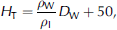
where ρ _W and ρ _I are the densities of water and ice, respectively, and H _T is the ice thickness at the terminus (D _W and H _T in metres). Changes in ice thickness in the terminal zone will cause the glacier to advance or retreat until Equation (3a) is again satisfied. Reference Vieli, Funk and BlatterVieli and others (2000, Reference Vieli, Funk and Blatter2001) adopted a modified calving margin criterion, replacing the fixed height-above-buoyancy value with a factor q:

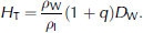
As currently formulated, neither calving-rate functions nor terminus position criteria are based on physical principles, and both have major drawbacks. There is currently no means of deriving values for parameters a and b in Equation (2) from the physical configuration of the glacier (e.g. ice thickness, width) or other relevant variables, thus limiting its utility as a general calving law. Conversely, the Van der Veen and Vieli height-above-buoyancy criteria cannot represent all types of calving margin, because they do not permit ice shelves to form. This is a major limitation in models where the build-up of marine ice sheets is of interest.

To overcome the limitations of existing calving laws, we introduce a new calving criterion based on a simple model of crevasse formation. In nature, calving occurs following fracture propagation under local (and often complex) stress conditions, and it is neither possible nor desirable to attempt to model individual events. Instead, we assume that calving is triggered by the downward propagation of transverse surface crevasses, which open in response to down-glacier variations in flow speed (longitudinal strain rates). While doubtless this is a simplification of reality, we argue that this mechanism represents an important first-order control on the position of the calving front, on which other ‘secondary’ calving processes are superimposed.

We calculate crevasse depth following Reference NyeNye (1957), by assuming that the base of a field of closely spaced crevasses lies at the depth where the longitudinal tensile strain rate (which tends to open crevasses) exactly balances creep closure resulting from the ice overburden pressure:

where g is gravitational acceleration, A and n are the flow-law parameters and ɛ is the longitudinal strain rate (∂U/∂x) minus the threshold strain rate required for crevasse initiation . We use the Nye formulation in preference to the more rigorous linear elastic fracture mechanics (LEFM) approach of Reference SmithSmith (1976), Reference Van der VeenVan der Veen (1998b) and Reference RistRist and others (1999), for three reasons. First, crevasse depths calculated using Reference Van der VeenVan der Veen’s (1998b) LEFM approach are highly sensitive to crevasse spacing, which is unknown a priori. Second, field data show that the Nye approach performs almost as well as that of Van der Veen at predicting observed crevasse depths (Mottram and Benn, unpublished data). Third, the much greater simplicity of the Nye formula makes it better suited for use in time-dependent ice-sheet models. Basal crevasses may also play a role in calving processes. However, theoretical analyses (Reference Van der VeenVan der Veen, 1998a) indicate that the height of penetration is likely to be small except for very high longitudinal strain rates and very low basal effective pressures, so their role is ignored here. Equation (4) assumes plane strain, which is compatible with the two-dimensional flowline model adopted here (see below). Choice of an appropriate value of ɛCRIT is difficult, because a wide range of values has been reported from laboratory and field studies (see Reference VaughanVaughan, 1993 for a review). Because our aim here is to outline the overall model structure, we adopt the simplifying assumption that and

Crevasses that are partially or wholly filled with water will penetrate deeper than predicted by Equation (4) because the ice overburden pressure tending to close the crevasse is opposed by water pressure (Reference RobinRobin, 1974; Reference Van der VeenVan der Veen, 1998a, Reference Van der Veenb). Incorporating the effect of water pressure into Equation (4) yields:

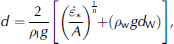
where d _W is the water depth in the crevasse. If the volume of water is fixed, d will have a stable value, but, if water is continually added to the crevasse, d will increase without limit and can eventually penetrate the full thickness of the glacier. Sustained water input can occur in response to surface melt or from supraglacial ponds (e.g. Reference Scambos, Hulbe, Fahnestock and BohlanderScambos and others, 2000; Reference Alley, Dupont, Parizek and AnandakrishnanAlley and others, 2005) or if a free connection exists between the crevasse and the proglacial water body, which is most likely if the crevasse is located close to the glacier margin. For present purposes, we assume that such a connection exists, so that surface crevasses will penetrate the full glacier thickness where they reach sea or lake level. In this case, the calving margin can be conveniently located where d equals the glacier ‘freeboard’ above sea level, h (Fig. 1):

Fig. 1.

Definition sketch of schematic calving terminus. The terminus may be either grounded (as shown) or floating, with any bed configuration.

where x is the horizontal coordinate parallel to glacier flow, positive downstream, L is glacier length and h = H - DW.

The down-glacier velocity gradient, ∂U/∂x, and the difference between ice thickness and water depth, h, are therefore considered to be the primary controls on glacier terminus position. The crevasse-depth calving criterion provides a simple physical explanation for the Van der Veen/Vieli height-above-buoyancy model, while allowing ice shelves to form. Where velocity gradients are high, crevasses will penetrate to the waterline before the glacier reaches flotation, producing a grounded calving front. On the other hand, where there are only small longitudinal velocity gradients near the grounding line, an ice shelf may form.

‘Sliding Laws’

The behaviour of calving glaciers depends critically on the ice velocity, for two reasons. First, ice velocity determines the rate at which ice is delivered to the calving front (Equation (1)), and is thus a primary control on calving flux. Second, longitudinal strain rate is the first derivative of velocity (Equation (5)), so down-glacier variations in velocity strongly influence both the terminus position (Equation (7)) and temporal changes in ice thickness by dynamic thinning. In this section we outline three alternative ‘sliding laws’, each of which has different implications for the location of the calving margin and glacier response to imposed thickness changes. We focus on flow along the centre line of an outlet glacier, with the x coordinate directed down-flow, and the z co-ordinate vertical, positive upward from sea or lake level. It is assumed that the shear stress components, τxy and τyz , the transverse deviatoric normal stress, σ′_yy and the transverse velocity, V, are zero.

Appropriate functions for calculating basal motion, U _B (which we take to include all basal processes, including sliding in the narrow sense and deformation of subglacial sediment), depend on the forces resisting flow. The force-balance approach developed by Van der Veen and Whillans (1987) defines the relationship between driving and resisting stresses as:

where τ _D is the driving stress, the first term on the righthand side is basal drag, the second term is resistance to flow arising from lateral drag, and the third term is resistance arising from longitudinal stress gradients. In the results reported here, the longitudinal stress gradient term is neglected (cf. Reference Van der VeenVan der Veen, 1999), and we focus on the role of basal and lateral drag in controlling the flow of calving glaciers.

Model 1 assumes that basal drag is the only non-zero resistance term:

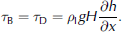
This assumption underpins the widely used ‘sliding law’ introduced by Reference Budd, Keage and BlundyBudd and others (1979):

where k is a sliding rate factor, P _E is the effective pressure and P and Q are empirically determined exponents. Widely varying values of k, P and Q have been reported in the literature (e.g. Reference BindschadlerBindschadler, 1983; Reference Raymond and HarrisonRaymond and Harrison, 1987; Reference Iken and TrufferIken and Truffer, 1997). To our knowledge, the only values determined for a tidewater glacier are those obtained for Columbia Glacier, Alaska, by Reference NickNick (2006): k = 9.2 ×106ma^–1 Pa^0.5, P = 3 and Q = 3.5, and these are adopted here. The effective pressure is the difference between ice overburden pressure, Pl = ρlgH, and basal water pressure, P _W. For a calving glacier where basal water flows towards the terminus, a minimum value for the basal water pressure is determined by the depth of the bed below sea level, Z _B. It is therefore useful to define the effective pressure in terms of this minimum value, plus an additional component ϕ associated with the subglacial transport and storage of meltwater:

(e.g. Reference Meier and PostMeier and Post, 1987; Reference Van der VeenVan der Veen, 1999). In the simplest model case, ϕ can be set to zero (cf. Reference Vieli, Funk and BlatterVieli and others, 2001), although this will tend to produce unrealistic velocity distributions, as discussed below. Values of ϕ can be modelled explicitly (cf. Reference Flowers and ClarkeFlowers and Clarke, 2002), or prescribed using an assumed piezometric gradient.

In model 2, all of the driving stress is supported by drag at the lateral margins. Shear stress at the margins, τ _S, is related to the driving stress, τ _D, by a factor that varies with channel geometry. For a rectangular channel the relationship is:

This approximates the situation in ice shelves and some ice streams (Reference Van der VeenVan der Veen, 1999). The centre-line velocity is calculated by integrating the flow law for ice from the flow-unit margins to the centre line:

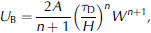
where W is the flow-unit half-width. From the definition of τ _D (Equation (11)), this is equivalent to:

Thus, velocity is independent of ice thickness, but if n = 3, centre-line velocity is proportional to the third power of the surface slope and the fourth power of the flow-unit width.

In model 3, resistance to flow is provided by a combination of basal and lateral drag. Theoretical sliding laws for this situation have been proposed by Reference RaymondRaymond (1996) and Reference Van der VeenVan der Veen and Whillans (1996). We derive a new sliding function by (1) scaling basal drag to the driving stress and basal water pressure and (2) using this value to derive a modified form of Equation (13). For step (1), we begin by assuming that τ _B = 0 when P _W = P _I and τ _B = τ _D when P _W = 0. Variation of _B between these limits is then defined by:

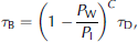
where C is a tuning parameter. In step (2), a sliding function is obtained by replacing τ _D in Equation (13) with the component of the driving stress that is not supported by basal drag,

This formulation implicitly assumes a rectangular cross-section, and that basal drag is constant across the bed. Equation (15) is similar to the dimensionless sliding function derived by Reference RaymondRaymond (1996), but with the advantage that the relationship between basal drag and effective pressure can be easily varied using a single parameter C. Preliminary experiments with the Columbia Glacier dataset presented by Reference KrimmelKrimmel (2001) indicate that a good fit between modelled and observed velocities can be obtained when C = 0.2, and reasonable values are used for the piezometric gradient (see below).

The velocity at the ice surface is the sum of basal motion and the cumulative velocity, U _I, resulting from vertical shear in the ice. For fast-flowing calving glaciers, the creep component can be assumed to be small compared to basal sliding, and in the work presented here we assume that the calculated basal velocity, U _B, is equal to the vertically averaged ice velocity, U. It is useful, however, to consider the implications of the assumptions of the three flow models for the calculation of ice creep velocities. In model 1, the implicit assumption that the driving stress is equal to an opposing basal drag leads to the unrealistic result that vertical shear will occur even when the basal effective pressure is very small. Calculated creep velocities, therefore, will be increasingly unrealistic as flotation is approached. In model 2, basal drag is zero, so no vertical shear occurs. This contrast between models 1 and 2 highlights the difficulty of coupling sheet-flow and ice-shelf models across the grounding line: the mutually exclusive assumptions of the models preclude any smooth transition between them. Model 3 overcomes this problem by dealing with both grounded and floating ice within a single framework. The strain rate in simple shear is given by the constitutive relation:

where τ _e is the effective stress, and

By scaling τxz to τ _B instead of τ _D, vertical shear strain will tend toward zero as basal drag vanishes, allowing a smooth transition between grounded and floating parts of the model domain. If it is assumed that . and the effective stress is given by:

The longitudinal deviatoric stress, σ′_xx is not known, but a first approximation can be obtained from the longitudinal strain rate derived from the basal velocity gradient. A consistent set of solutions for Equations (16), (18) and U _B can then be obtained iteratively.

Coupling Calving and Sliding Laws

We now examine the behaviour of the crevasse-depth calving law coupled with the three alternative sliding laws (Equations (10), (13) and (15)), by analyzing how flow speed, terminus position and dynamic thinning rates respond to imposed changes in ice thickness and flow-unit width. Change in ice thickness through time is obtained from the continuity equation:

where the first term on the righthand side is the surface or basal mass balance (accumulation positive, ablation negative), the second term represents the advection of thicker ice from up-glacier (advective thickening), the third term is dynamic thinning (thickening) resulting from longitudinal stretching (shortening), and the fourth term is dynamic thinning (thickening) resulting from flow divergence (convergence) in the y (transverse) direction (on a flowline, the advective thickening term in the y direction is zero). By assuming that ice in a widening channel remains in contact with the sides, the transverse divergence term can be expressed in terms of the velocity in the x direction, U, and half-width, W:

(Reference SandersonSanderson, 1979; Reference Van der VeenVan der Veen, 1999).

When U is calculated using model 1, ice velocity increases as ice thickness decreases towards the flotation thickness. Velocities calculated from ice thickness, water depth and surface slope values representative of the terminal zone of Columbia Glacier in 1988 (when fast flow was well established and terminus retreat was in progress) are shown in Figure 2a. In the example shown, it is assumed that ϕ = 0 (Equation (11)), equivalent to a horizontal piezometric surface at sea level. As ice thickness decreases, modelled velocity increases non-linearly. The non-linear increase in velocity means that the longitudinal velocity gradient, ∂U/∂x, also increases as ice becomes thinner (Fig. 2b), with the result that modelled crevasse depths also increase as the glacier thins towards the waterline (Fig. 2c). Because ∂U/∂x tends towards infinity as P _E approaches zero, the equality d = h will always be met while the glacier is still grounded. Thus, the physically impossible solution to Equation (10) – a floating ice shelf with an infinite velocity – is precluded because the calving criterion predicts that crevasses will penetrate the full thickness of the glacier before flotation occurs. In the present example, the model predicts that the terminal ice cliff is 65–77m high, and that the ice velocity at the terminus (and hence calving rate) is 2.2–3.2 km a^–1, depending on fjord water salinity. The modelled calving rate is lower than the observed value of ~5.4 kma^–1. There are several possible reasons for this discrepancy, including the unrealistic assumption that ϕ = 0 throughout the glacier tongue (cf. Reference MeierMeier and others, 1994). Similar values for terminal ice cliff height and more realistic calving rates can be obtained using a piezometric gradient of 0.005 mm^–1. The impact of piezometric gradient on modelled velocities, strain rates and calving rates is discussed in greater detail below, with respect to model 3.

Fig. 2.

Model 1: (a–c) relationships between ice thickness and (a) velocity, (b) longitudinal strain rate and (c) crevasse depth; and (d) relationship between normalized height above buoyancy and dynamic thickening rate. Z _B = 400 m; surface slope = 1.158; water density = 1030 kgm^–3 (solid dark lines) and 1000 kgm^–3 (dashed lines). The calving margin is located where the ice height above the waterline (dotted line in (c)) equals crevasse depth.

Modelled velocities, strain rates and crevasse depths are all greater for glaciers terminating in sea water (ρ _W = 1030 kgm^–3) than fresh water (ρ _W = 1000 kgm^–3), for any given ice thickness (Fig. 2). This is because a greater density difference between ice and the proglacial water body has a large effect on the maximum possible effective pressure at the glacier bed, and hence ice velocities (Reference Van der VeenVan der Veen, 2002). For any given combination of ice thickness and water depth, greater amounts of ice will be delivered to a tidewater calving front than a freshwater one, explaining the oft-noted contrast in water-depth–calving-rate functions between marine and lake-terminating glaciers (e.g. Reference WarrenWarren, 1992; Reference Van der VeenVan der Veen, 1996, Reference Van der Veen2002).

When output from model 1 is inserted into the continuity equation (19), an interesting pattern emerges. Because ice velocity increases as ice approaches flotation, the advective thickening term increases down-glacier (Fig. 2d, upper curve). However, thinning in response to longitudinal stretching increases much more rapidly as ice thickness decreases (Fig. 2d, lower curve). For the 1988 Columbia Glacier terminus geometry, the continuity equation predicts strong dynamic thinning, increasing exponentially as the glacier approaches flotation. This provides a possible explanation for the observed rapid retreat of Columbia Glacier: an imposed thinning (due, for example, to increased melting) will trigger accelerated ice flow and dynamic thinning, which could then become a self-sustaining process. A dynamic thinning feedback will trigger terminus retreat because (1) as ice thickness decreases, it is increasingly likely that crevasses will penetrate down to the waterline, and (2) increased longitudinal strain rates result in deeper crevasses. In combination, these two effects will cause the glacier terminus to retreat up-glacier until it is able to stabilize in shallower water. Any tendency to dynamic thinning will be increased if the channel width increases downstream, and damped if it decreases due to the lateral divergence term in the continuity equation (Equations (19) and (20)). Thus, despite its simple formulation, model 1 successfully exhibits the well-known tendency for calving glaciers to stabilize at ‘pinning points’ (e.g. narrow or shallow sections of a fjord), and to retreat rapidly between pinning points during periods of negative mass balance (cf. Reference Vieli, Funk and BlatterVieli and others, 2000, Reference Vieli, Funk and Blatter2001). The model also predicts that sensitivity to imposed thinning is stronger for tidewater than freshwater-terminating glaciers.

In model 2, where ice velocity is controlled entirely by lateral drag, glacier response to changes in ice thickness and channel width contrasts markedly with model 1. Imposed glacier thinning will not result in flow acceleration unless thinning is also associated with an increase in surface slope. The lack of a direct relationship between ice thickness and velocity means that ice can become fully buoyant without experiencing the high longitudinal velocity gradients required for crevasse propagation and calving failure. In contrast, ice velocity is proportional to the third power of surface slope and the fourth power of channel width (for n = 3; Fig. 3). Thus, flow acceleration will occur if the glacier steepens, and particularly strong acceleration will occur at channel widenings. Where W increases, accelerating flow leads to longitudinal stretching, so that crevasses are likely to penetrate to the waterline and trigger calving failure at such locations. This sensitivity to channel width is much stronger than in model 1, in which velocity is influenced by W only through the lateral divergence term in the continuity equation. This feature of model 2 provides the most likely explanation for the tendency for tidewater glacier and ice-shelf margins to be located at topographic widenings.

Fig. 3.

Model 2: centre-line velocity as a function of channel half-width, W, and surface gradient.

In model 3, sliding velocity is sensitive to changes in both ice thickness relative to water depth and channel width. Figure 4 illustrates the behaviour of the combined basal– lateral-drag ‘sliding law’ (Equation (15)) using ice-thickness and driving-stress values representative of the 1988 Columbia Glacier geometry, and C = 0.2. The half-width of the glacier terminus was ~2.5 km at that time, and it can be seen that the model predicts velocities in the correct range (~5kma^–1) when P _w/P _I ≈ 0.95. Like model 1, velocities increase non-linearly as basal water pressure approaches the ice pressure (i.e. as basal drag tends towards zero), but unlike model 1 velocities have a finite value when flotation occurs. This means that calving will not necessarily occur before the terminus goes afloat (as in model 1), but will depend on the spatial scale over which τ _B vanishes. If basal drag diminishes rapidly as the ice approaches flotation, calving will occur while the ice is still grounded, whereas if the transition from high to low values of τ _B occurs over a long distance, high longitudinal strain rates are avoided and an ice shelf can form. Thus, lateral drag potentially has a stabilizing effect on calving glacier termini.

Fig. 4.

Model 3: centre-line velocity as a function of P _W/P _I and Wτ _D = 95 kPa, H = 480 m, C = 0.22 (values representative of the marginal zone of Columbia Glacier in 1988).

Modelled velocity gradients, crevasse depths and dynamic thickening rates for the Columbia Glacier example are shown in Figure 5. Figure 5a, c and e show results for ϕ = 0 (horizontal piezometric surface at sea level), and Figure 5b, d and f show results for the more realistic situation of ϕ rising up-glacier (equivalent to a piezometric gradient of 0.012, chosen to achieve the best fit with the observed velocities). Allowing ϕ to rise up-glacier has the effect of reducing modelled longitudinal strain rates and crevasse depths relative to the ϕ = 0 case. Both model runs over-predict glacier length, and calving does not occur until the glacier is within ~0.98 of flotation. In physical terms, this over-prediction may reflect deficiencies in the crevasse depth model, or the omission of important factors such as longitudinal stress gradients, surface meltwater entering crevasses, or ‘secondary’ calving processes associated with longitudinal stress gradients in the immediate vicinity of the ice front (cf. Reference O’Neel, Echelmeyer and MotykaO’Neel and others, 2003). Despite these difficulties, however, the model performs remarkably well at predicting the approximate position of the calving margin. Figure 5e and f show calculated dynamic thinning rates for the two modelled cases. The thinning tendency is greater for ϕ = 0, because of higher longitudinal stretching rates, but in both cases the model indicates that the glacier terminus is unstable and ‘locked into’ a self-reinforcing thinning process. We propose that this modelled behaviour captures the fundamental process responsible for the observed behaviour of Columbia and other tidewater glaciers: an imposed thinning triggers a positive feedback between acceleration, dynamic thinning and calving retreat. Importantly, the model predicts that this feedback is much less likely to operate where surface gradients are low, basal drag diminishes over large distances, and lateral drag provides most resistance in the vicinity of the grounding line. Thus, model 3 suggests that water-terminating glaciers will tend to be potentially unstable if basal drag provides most resistance to flow in the terminal zone, and stable if most resistance is provided by lateral drag.

Fig. 5.

Velocities (a, b), crevasse depths (c, d) and dynamic thinning rates (e, f) calculated from model 3, using the same input values as in Figure 4, assuming a horizontal piezometric surface (a, c, e), and a piezometric surface rising up-glacier (b, d, f).

Centre-line velocities calculated from Equation (15) are also highly sensitive to changes in glacier width (Fig. 4). High longitudinal strain rates and deep crevasses will therefore occur at widenings of fjords and embayments, making it likely that calving margins will be located in such places. Conversely, where W decreases down-glacier, velocity will decrease for any given value of the driving stress. Of course, continuity requires that dynamic thickening must occur if W and U both decrease; this tendency means that the driving stress will increase until sufficient ice is discharged through the constriction.

In its present form, model 3 does not include longitudinal stress gradients. Higher-order modelling by Reference Payne, Vieli, Shepherd, Wingham and RignotPayne and others (2004) and Reference HindmarshHindmarsh (2006) suggests that this term in the force balance plays an important role in modulating the transition between equilibrium states, and further work is required to establish where and when the assumptions of model 3 are appropriate. Nevertheless, model 3 represents a considerable improvement on existing methods of representing calving processes and their relationship with ice dynamics, and has the potential to explain and simulate many elements of the observed behaviour of calving glaciers.

Conclusions

A simple physically based calving law, which defines the position of the glacier terminus as the point where crevasse depth equals the ice ‘freeboard’ above sea level, provides a more flexible and robust marine boundary condition for ice-sheet models than existing calving laws.

Terminus retreat can be triggered either by increases in longitudinal strain rates (which cause deeper crevasses), or by decreases in ice thickness (which increase the likelihood that crevasses will reach the waterline).

Modelled glacier dynamics depends critically on the choice of sliding law. Where sliding velocity is inversely proportional to effective pressure, any imposed thinning on a calving glacier will lead to ice acceleration and retreat of the calving front because effective pressure is influenced by water depth. Feedbacks between ice thickness, sliding velocity and dynamic thinning provide a powerful means of amplifying initial signals. Increased melting in the terminal zone can trigger acceleration, thinning and terminus retreat. This scenario was modelled by Reference Vieli, Funk and BlatterVieli and others (2001) and suggests that, where resistance to flow is mainly from basal drag, calving glaciers are highly sensitive to external triggers, because of the dynamical instability of the system as ice approaches flotation.

In contrast, where all resistance to flow is provided by lateral drag, ice velocity is insensitive to imposed thickness changes, unless these are associated with changes in ice surface gradient. The position of the calving front is strongly influenced by topography, because ice velocity is proportional to the fourth power of channel half-width. Channel widening will therefore result in higher ice velocities and longitudinal strain rates, increasing the likelihood that the calving margin will occur at such locations. Outlet glaciers and ice streams controlled by lateral drag should be insensitive to imposed thickness changes, and be relatively stable.

A new sliding function is proposed that parameterizes the effects of both lateral and basal drag. This model exhibits sensitivity to imposed thickness changes, but the stabilizing effects of lateral drag mean that the system will not necessarily exhibit dynamic instability as the glacier approaches flotation. Ice shelves will form where reduction of basal drag (and the corresponding flow acceleration and longitudinal strain rates) occurs over a sufficiently long spatial scale. This analysis yields significant new insights into the essential features of calving margins, which can be tested against new observations.