





1. Introduction
The boundary-layer transition from a laminar to a turbulent state could significantly impact high-speed vehicle design. Despite substantial progress over the past decades, predicting supersonic boundary-layer transition remains challenging due to complex physical processes. Under small-amplitude free stream disturbances, transition usually follows three stages: (1) receptivity; (2) linear growth and (3) nonlinear breakdown to turbulence. Receptivity is the process by which free stream disturbances enter the boundary layer and excite instability waves that travel within the boundary layer. For flat plates or sharp cones at zero angle of attack, typical examples of these waves are the first and second mode instabilities (Mack Reference Mack1984; Schneider Reference Schneider2004), which are commonly referred to as modal instabilities. These waves subsequently undergo a phase of linear growth until their amplitudes become sufficiently large for nonlinear effects to dominate, ultimately leading to turbulent breakdown.
The leading edges of high-speed vehicles are typically designed with some degree of bluntness to reduce surface heat flux. This geometry generates a bow shock followed by an entropy layer that thickens as the nose radius increases. Linear stability theory (LST) (Mack Reference Mack1984) has shown that the entropy layer can delay transition by stabilising the modal instabilities (Malik, Spall & Chang Reference Malik, Spall and Chang1990). Therefore, the transition location should continuously move downstream with increasing nose radius according to LST. When the nose radius is small, this prediction is consistent with the findings of Stetson’s experiments (Stetson & Rushton Reference Stetson and Rushton1967; Stetson Reference Stetson1983). The experiments also demonstrated that the downstream movement of the transition location slows as the bluntness increases and the trend reverses once the nose radius exceeds a certain threshold. This phenomenon is commonly known as transition reversal, and has also been observed in other transition experiments for blunt cones (Zanchetta et al. Reference Zanchetta, Hillier, Henkes and van Ingen1996; Marineau et al. Reference Marineau, Moraru, Lewis, Norris, Lafferty, Wagnild and Smith2014; Paredes et al. Reference Paredes, Choudhari, Li, Jewell, Kimmel, Marineau and Grossir2019b ; Ceruzzi et al. Reference Ceruzzi, Le Page, McQuellin, Condren and McGilvray2025), blunted plates (Lysenko Reference Lysenko1990; Aleksandrov et al. Reference Aleksandrov, Aleksandrova, Borovoy, Gubernatenko, Mosharov, Radchenko, Skuratov, Fedorov and Chuvakhov2019; Borovoy et al. Reference Borovoy, Radchenko, Aleksandrov and Mosharov2022) and ogive cylinders (Hill et al. Reference Hill, Oddo, Komives, Reeder, Borg and Jewell2022). Another type of modal instability, known as the entropy mode, has been reported to exhibit a marginal growth rate (Dietz & Hein Reference Dietz and Hein1999; Chen et al. Reference Chen, Tu, Wan, Su, Yuan and Chen2021), which does not help to explain the transition reversal. Therefore, while LST can predict transition delay due to the increase in bluntness, it fails to account for transition reversal.
One proposed explanation for transition reversal is that it is caused by disturbances originating from surface roughness near the nose. In Stetson’s experiments (Stetson Reference Stetson1983), for cases with a large nose radius, polishing the surface delayed transition or resulted in fully laminar flow. In contrast, it had no significant impact on the transition location for cases with small nose radii. In the experiments by Paredes et al. (Reference Paredes, Choudhari, Li, Jewell, Kimmel, Marineau and Grossir2019b ), surface roughness located near the sonic point at the nose significantly promoted the transition on the cone with the blunter nose, while having no effect on the transition location on the sharper cone. They concluded that the transition onset in the blunter nose case results from the combined effects of roughness and nose bluntness. Borovoy et al. (Reference Borovoy, Radchenko, Aleksandrov and Mosharov2022) showed that polishing the nose shifts the transition zone downstream for largely blunted plates, which was believed to be the result of a decrease in the disturbance level near the junction of the nose and the plate. However, surface polishing did not eliminate the transition reversal in these experiments. Therefore, although surface roughness may affect the transition location in cases of large bluntness, more research is needed to understand how it is involved in the transition reversal.
Many experimental results also suggest that there is a shift in the dominant instability as the nose radius is increased. In the experiments by Grossir et al. (Reference Grossir, Pinna, Bonucci, Regert, Rambaud and Chazot2014, Reference Grossir, Pinna and Chazot2019) for blunt cones in Mach 10 flow, the structures of the disturbances for cases with large nose radii differed from the rope-like structure associated with the second mode instability. The results of Jagde et al. (Reference Jagde, Kennedy, Laurence, Jewell and Kimmel2019) and Kennedy et al. (Reference Kennedy, Jagde, Laurence, Jewell and Kimmel2019) revealed that the rope-like structures of the second mode for sharp cones changed to wisp-like structures as the bluntness of the nose increased. For ogive cylinders, Hill et al. (Reference Hill, Oddo, Komives, Reeder, Borg and Jewell2022) showed that the primary disturbance structure in the boundary layer could be rope-like, elongated or wisp-like, depending on the bluntness of the tip and the curvature of the ogive. The rope-like structures correspond to the second-mode instability, while the other two remain unexplained.
Due to the failure of the modal instability analysis (such as LST) to predict transition reversal, efforts were made to study the role of non-modal instabilities in the transition process. Paredes et al. (Reference Paredes, Choudhari, Li, Jewell and Kimmel2019a ,Reference Paredes, Choudhari, Li, Jewell, Kimmel, Marineau and Grossir b ) attempted to use optimal transient growth analysis to explain transition in the experiments by Jewell et al. (Reference Jewell, Kennedy, Laurence and Kimmel2018) for blunt cones. It was shown that stationary three-dimensional disturbances initiated near the nose could undergo significant non-modal amplification. These disturbances corresponded to three-dimensional stationary streaks and weakened with increases in nose radius. Paredes et al. (Reference Paredes, Choudhari, Li, Jewell and Kimmel2019a ) also identified non-stationary three-dimensional and planar disturbances travelling inside the entropy layer and above the edge of the boundary layer. The non-modal amplification of these disturbances was lower than that for the three-dimensional stationary disturbances, but increased as the nose radius increased. Scholten et al. (Reference Scholten, Goparaju, Gaitonde, Paredes, Choudhari and Li2022) used modal and non-modal analysis to study instabilities in hypersonic flow over blunted plates, where the configurations are the same as those of Lysenko (Reference Lysenko1990). The amplification of non-modal disturbances in the entropy layer increases when the nose radius is increased from small to moderate and their magnitude becomes comparable to the magnitude of modal instabilities. However, such amplification decreases as the nose radius increases further.
Computational fluid dynamics has also been a popular method for studying the supersonic/hypersonic transition on blunt bodies in recent decades. Paredes, Choudhari & Li (Reference Paredes, Choudhari and Li2020) studied the transition scenario on a blunt cone with a moderately blunt nose. It was demonstrated that nonlinear interactions between disturbances travelling inside the entropy layer can generate stationary streaks that penetrate and amplify within the boundary layer, leading to transition through streak breakdown. Goparaju & Gaitonde (Reference Goparaju and Gaitonde2022) investigated the effects of entropy layer instabilities on a moderately blunted plate at Mach 4. They suggested that the oblique breakdown of the entropy layer instabilities, which amplify via lift-up and Orr-like mechanisms, could lead to the onset of transition. Zhu et al. (Reference Zhu, Li, Guo, Liu and Tong2023) and Aswathy Nair & Unnikrishnan (Reference Aswathy Nair and Unnikrishnan2024) numerically investigated the effect of the nose radius on the transition location on a blunt cone and an ogive cylinder, respectively. In these simulations, disturbances were introduced downstream of the nose, which means that the receptivity of the nose, which could play an important role in the transition reversal, was not considered. This may explain why transition reversal was not observed in either study. Goparaju, Unnikrishnan & Gaitonde (Reference Goparaju, Unnikrishnan and Gaitonde2021) used a two-dimensional direct numerical simulation (DNS) investigation to study the effect of the nose radius on a Mach 6 boundary layer over a blunted plate. With random pressure noise placed upstream of the bow shock, they reported a reversal in the growth rate of the most amplified waves as the nose radius increased. Melander, Dwivedi & Candler (Reference Melander, Dwivedi and Candler2022) performed DNS of Mach 6 flow over 8-degree blunt cones with nose radii of 1.524 and 15.24 mm. White noise was added as the free stream disturbance and low-frequency streaks were observed in both cases. In addition, the streaks became stronger as the nose radius increased. More recently, Guo, Hao & Wen (Reference Guo, Hao and Wen2025) performed high-fidelity simulations of Mach 5 flow over blunted plates with various nose radii. Broadband slow acoustic waves were used to trigger the transition. Transition reversal was reproduced in the simulations. For the sharp leading-edge case, the transition was induced by the second mode instability. For blunted plates, the transitions were caused by low-frequency streamwise streaks, which increased in magnitude as the nose radius increased. They concluded that the enhancement of streamwise streaks was responsible for the transition reversal and attributed the enhancement to the increase in the initial streak amplitude with increasing bluntness. However, the mechanisms underlying streak generation and amplification were not explored, and small to moderate nose radii were not considered. In a follow-up study, Guo (Reference Guo2025) examined the roles of other disturbances, specifically fast acoustic waves, entropy waves and vortical waves. The results show that for a blunted plate with its radius larger than the critical radius, all types of free stream disturbances, including slow acoustic waves, result in a ‘streamwise streak-turbulent spot’ two-stage transition scenario. Entropy waves were found to induce the earliest transition, followed by fast acoustic waves, slow acoustic waves and, finally, vortical waves. However, as only a single nose radius was investigated in that study, the question of whether other types of disturbances (fast acoustic, vortical and entropy waves) would also lead to transition reversal remains unaddressed. Based on these previous works, we can conclude that the receptivity process plays a key role in the transition reversal.
Owing to its importance, many numerical studies also focus on the receptivity process. For example, Zhong (Reference Zhong2005, Reference Zhong2009) conducted axisymmetric simulations of hypersonic flow over blunt cones with various nose radii, using free stream conditions corresponding to those in Stetson’s experiments (Stetson & Rushton Reference Stetson and Rushton1967; Stetson Reference Stetson1983). Balakumar & Kegerise (Reference Balakumar and Kegerise2011) investigated the receptivity of blunt wedges and cones to free stream acoustic and vorticity waves with different incident angles. The results show that the boundary layer is more receptive to slow acoustic waves than fast acoustic or vorticity waves, and the maximum receptivity of slow acoustic waves is obtained when the incident angle is $20^\circ$
. Zhao & Dong (Reference Zhao and Dong2025) employed the shock-fitting harmonic linearised Navier–Stokes (SFHLNS) equations to study the effects of nose bluntness on receptivity to various kinds of free stream disturbances. They found that free stream acoustic and entropy disturbances are more effective in triggering non-modal streaky disturbances than free stream vortical disturbances. In addition, the receptivity efficiency increases with nose bluntness for acoustic and entropy disturbances, and decreases for vortical disturbances. However, only three nose radii were considered in their cases and the underlying mechanisms of streak generation were not explored. More importantly, the role of the receptivity of the nose remains unclear in the transition reversal phenomenon.
$20^\circ$
. Zhao & Dong (Reference Zhao and Dong2025) employed the shock-fitting harmonic linearised Navier–Stokes (SFHLNS) equations to study the effects of nose bluntness on receptivity to various kinds of free stream disturbances. They found that free stream acoustic and entropy disturbances are more effective in triggering non-modal streaky disturbances than free stream vortical disturbances. In addition, the receptivity efficiency increases with nose bluntness for acoustic and entropy disturbances, and decreases for vortical disturbances. However, only three nose radii were considered in their cases and the underlying mechanisms of streak generation were not explored. More importantly, the role of the receptivity of the nose remains unclear in the transition reversal phenomenon.
While many studies suggest that the transition reversal may result from the strengthening of non-modal disturbances as the nose radius increases, the development of such disturbances near the leading edge remains unexplored. First, the detailed generation and early evolution of these disturbances, particularly within the blunt leading-edge region, are not fully understood. Second, the role of leading-edge receptivity requires further clarification; specifically, it remains unclear whether the strengthening of streaks responsible for transition reversal requires free stream disturbances interacting with the bow shock and nose, or whether similar amplification can be produced by disturbances introduced downstream of the shock. Finally, it is yet to be determined whether other realistic free stream disturbances, such as entropy and vorticity waves, can also induce transition reversal and how they might alter the critical nose radius. To address these gaps, the present study investigates the receptivity of supersonic flow over blunted flat plates to various free stream disturbances using the linearised Navier–Stokes equations (LNSEs). The study primarily focuses on free stream slow acoustic waves, which are the dominant component of wind tunnel noise (Duan et al. Reference Duan2019). Furthermore, to reflect actual free-flight conditions, the receptivity to free stream entropy and vorticity waves is also analysed. In addition to the LNSE, resolvent analysis is employed to assess the importance of leading-edge receptivity by comparing the flow’s response to forcing applied in the free stream versus downstream of the shock. This paper is organised as follows: § 2 details the flow conditions and geometry; § 3 outlines the numerical methods; § 4 presents and discusses the results; and § 5 concludes the study.
Schematic drawing of the computational domain.

Figure 1. Long description
A schematic drawing of the computational domain. The diagram represents the flow around a blunt leading edge of a high-speed vehicle. It includes a symmetry boundary at the bottom, a no-slip isothermal wall boundary along the surface, and an outflow boundary at the right side. The flow enters from the left with specified freestream conditions, including Mach number, temperature, density, and Reynolds number. Disturbances are introduced at an angle theta. Two forcing locations are marked along the flow path, with forcing location 1 closer to the leading edge and forcing location 2 further downstream. A bow shock forms ahead of the leading edge, and a response region is indicated downstream of the forcing locations. The diagram also shows the coordinates x, y, and eta, with Rn representing the nose radius.
2. Problem description
This work considers supersonic flow over flat plates with cylindrically blunted noses of various radii $\tilde {R}_n$
. A schematic diagram is provided in figure 1. The symbol
$\tilde {R}_n$
. A schematic diagram is provided in figure 1. The symbol $\tilde {(\boldsymbol{\cdot })}$
refers to dimensional quantities and
$\tilde {(\boldsymbol{\cdot })}$
refers to dimensional quantities and $(\boldsymbol{\cdot })_{\infty }$
represents free stream quantities. A Cartesian coordinate system
$(\boldsymbol{\cdot })_{\infty }$
represents free stream quantities. A Cartesian coordinate system $(x, y, z)$
is defined with the origin located at the centre of the nose, the
$(x, y, z)$
is defined with the origin located at the centre of the nose, the $x$
-axis aligned horizontally, the
$x$
-axis aligned horizontally, the $y$
-axis aligned vertically and the
$y$
-axis aligned vertically and the $z$
-axis following the right-hand rule. The corresponding velocities are denoted by
$z$
-axis following the right-hand rule. The corresponding velocities are denoted by $u$
,
$u$
, $v$
and
$v$
and $w$
hereafter. In addition, a body-fitted coordinate system
$w$
hereafter. In addition, a body-fitted coordinate system $(\xi , \eta )$
is constructed, where
$(\xi , \eta )$
is constructed, where $\xi$
is along the body surface and
$\xi$
is along the body surface and $\eta$
represents the wall-normal direction. The free stream conditions are as follows: Mach number
$\eta$
represents the wall-normal direction. The free stream conditions are as follows: Mach number $ M_{\infty } = 4$
; free stream temperature
$ M_{\infty } = 4$
; free stream temperature $ \tilde {T}_{\infty } = 69.05\,\mathrm{K}$
; free stream density
$ \tilde {T}_{\infty } = 69.05\,\mathrm{K}$
; free stream density $ \tilde {\rho }_{\infty } = 0.259\,\mathrm{kg\,m^{-3}}$
and unit Reynolds number
$ \tilde {\rho }_{\infty } = 0.259\,\mathrm{kg\,m^{-3}}$
and unit Reynolds number $ \tilde{\textit{Re}}_{\infty } = 37 \times 10^6$ $ \mathrm{m}^{-1}$
. These free stream conditions are taken from the experiments by Lysenko (Reference Lysenko1990). The wall temperature
$ \mathrm{m}^{-1}$
. These free stream conditions are taken from the experiments by Lysenko (Reference Lysenko1990). The wall temperature $\tilde {T}_{{w}}$
is fixed at
$\tilde {T}_{{w}}$
is fixed at $ 255.48\,\mathrm{K}$
. The angle of incidence of the disturbance is denoted by
$ 255.48\,\mathrm{K}$
. The angle of incidence of the disturbance is denoted by $\theta$
, which is defined to be positive for a disturbance wave impinging on the model from above.
$\theta$
, which is defined to be positive for a disturbance wave impinging on the model from above.
Lysenko (Reference Lysenko1990) reported that the critical nose radius for transition reversal was approximately 0.5 mm and the transition onset location was approximately 110 mm. Accordingly, the present study examines six nose radii, $\tilde {R}_n = 0.1, 0.2, 0.5, 0.7, 1$
and 2 mm, with a fixed plate length of
$\tilde {R}_n = 0.1, 0.2, 0.5, 0.7, 1$
and 2 mm, with a fixed plate length of $\tilde {L}_{{p}} = 200$
mm for all cases. Table 1 summarises the grid resolutions and case nomenclature. The baseline cases are named according to their nose radii (e.g. R01 for
$\tilde {L}_{{p}} = 200$
mm for all cases. Table 1 summarises the grid resolutions and case nomenclature. The baseline cases are named according to their nose radii (e.g. R01 for $\tilde {R}_n = 0.1$
mm). For receptivity studies involving slow acoustic, entropy and vorticity waves, the subscripts
$\tilde {R}_n = 0.1$
mm). For receptivity studies involving slow acoustic, entropy and vorticity waves, the subscripts $(\boldsymbol{\cdot })_{A}$
,
$(\boldsymbol{\cdot })_{A}$
, $(\boldsymbol{\cdot })_{E}$
and
$(\boldsymbol{\cdot })_{E}$
and $(\boldsymbol{\cdot })_{V}$
are appended to the baseline case names, respectively. In these cases, the incidence angle
$(\boldsymbol{\cdot })_{V}$
are appended to the baseline case names, respectively. In these cases, the incidence angle $\theta$
is set to
$\theta$
is set to $0^\circ$
. To investigate the influence of the incidence angle for slow acoustic waves, additional simulations are performed with
$0^\circ$
. To investigate the influence of the incidence angle for slow acoustic waves, additional simulations are performed with $\theta$
ranging from
$\theta$
ranging from $10^\circ$
to
$10^\circ$
to $60^\circ$
. To reduce computational cost, these simulations are restricted to three nose radii:
$60^\circ$
. To reduce computational cost, these simulations are restricted to three nose radii: $\tilde {R}_n = 0.1, 0.7$
and 2 mm. These cases are identified by the subscript
$\tilde {R}_n = 0.1, 0.7$
and 2 mm. These cases are identified by the subscript $(\boldsymbol{\cdot })_S$
.
$(\boldsymbol{\cdot })_S$
.
Flow conditions, number of grid points and geometry configuration of the blunted plate for different cases.

Table 1. Long description
A table comparing flow conditions, number of grid points, and geometry configuration for different blunted plate cases. The table has 12 rows and 9 columns. Column headers are: M infinity, T infinity (K), rho infinity (kg m^-3), Re infinity (m^-1), Case name, Rn (mm), Re Rn, Nx, Ny, Lp (mm). Row 1: M infinity, 4; T infinity (K), 69.05; rho infinity (kg m^-3), 0.259; Re infinity (m^-1), 37.0 x 10^6; Case name, R01; Rn (mm), 0.1; Re Rn, 3701.75; Nx, 3281; Ny, 641; Lp (mm), 200. Row 2: M infinity, 4; T infinity (K), 69.05; rho infinity (kg m^-3), 0.259; Re infinity (m^-1), 37.0 x 10^6; Case name, R02; Rn (mm), 0.2; Re Rn, 7403.50; Nx, 3301; Ny, 641; Lp (mm), 200. Row 3: M infinity, 4; T infinity (K), 69.05; rho infinity (kg m^-3), 0.259; Re infinity (m^-1), 37.0 x 10^6; Case name, R05; Rn (mm), 0.5; Re Rn, 18508.75; Nx, 3351; Ny, 641; Lp (mm), 200. Row 4: M infinity, 4; T infinity (K), 69.05; rho infinity (kg m^-3), 0.259; Re infinity (m^-1), 37.0 x 10^6; Case name, R07; Rn (mm), 0.7; Re Rn, 25912.25; Nx, 3371; Ny, 641; Lp (mm), 200. Row 5: M infinity, 4; T infinity (K), 69.05; rho infinity (kg m^-3), 0.259; Re infinity (m^-1), 37.0 x 10^6; Case name, R1; Rn (mm), 1.0; Re Rn, 37017.50; Nx, 3401; Ny, 641; Lp (mm), 200. Row 6: M infinity, 4; T infinity (K), 69.05; rho infinity (kg m^-3), 0.259; Re infinity (m^-1), 37.0 x 10^6; Case name, R2; Rn (mm), 2.0; Re Rn, 74035.00; Nx, 3601; Ny, 641; Lp (mm), 200. Row 7: M infinity, 4; T infinity (K), 69.05; rho infinity (kg m^-3), 0.259; Re infinity (m^-1), 37.0 x 10^6; Case name, R01s; Rn (mm), 0.1; Re Rn, 3701.75; Nx, 6561; Ny, 641; Lp (mm), 200. Row 8: M infinity, 4; T infinity (K), 69.05; rho infinity (kg m^-3), 0.259; Re infinity (m^-1), 37.0 x 10^6; Case name, R07s; Rn (mm), 0.7; Re Rn, 25912.25; Nx, 6741; Ny, 641; Lp (mm), 200. Row 9: M infinity, 4; T infinity (K), 69.05; rho infinity (kg m^-3), 0.259; Re infinity (m^-1), 37.0 x 10^6; Case name, R2s; Rn (mm), 2.0; Re Rn, 74035.00; Nx, 7201; Ny, 641; Lp (mm), 200.
The grids are clustered near the wall, the leading edge and the shock. Near the wall, the grid is distributed such that approximately 60 % of the grid points are within the boundary layer. For simulations with non-zero $\theta$
, the grid is mirrored about the body symmetry line, doubling the number of streamwise points,
$\theta$
, the grid is mirrored about the body symmetry line, doubling the number of streamwise points, $N_x$
. A grid independence study was performed to ensure numerical accuracy and the details are presented in Appendix A. For all simulations in this work, the shock wave is handled by the shock-capturing approach (see § 3). Therefore, the grid is carefully tailored to align with the shock wave to minimise numerical noise near the shock.
$N_x$
. A grid independence study was performed to ensure numerical accuracy and the details are presented in Appendix A. For all simulations in this work, the shock wave is handled by the shock-capturing approach (see § 3). Therefore, the grid is carefully tailored to align with the shock wave to minimise numerical noise near the shock.
3. Numerical methods
3.1. Governing equations
The governing equations are the non-dimensional three-dimensional compressible N–S equations, which are given as
 \begin{align} \frac {\partial\kern-1pt\boldsymbol{Q}}{\partial t}+\frac {\partial\kern-1pt\boldsymbol{F}_{\kern-1.5pt j}}{\partial x_{\kern-1pt j}}+\frac {\partial\kern-1pt\boldsymbol{F}_{\kern-1pt v j}}{\partial x_{\kern-1pt j}}=0, \end{align}
where ( $x_1, x_2, x_3$
) = (
$x_1, x_2, x_3$
) = ( $x, y, z$
). The vector of conservative variables
$x, y, z$
). The vector of conservative variables $\boldsymbol{Q}$
, the inviscid flux
$\boldsymbol{Q}$
, the inviscid flux $\boldsymbol{F}_{\kern-1.5pt j}$
and the viscous flux
$\boldsymbol{F}_{\kern-1.5pt j}$
and the viscous flux $\boldsymbol{F}_{vj}$
are given as
$\boldsymbol{F}_{vj}$
are given as
 \begin{align} \boldsymbol{Q}=\left [\begin{array}{c} \rho \\ \rho u_1 \\ \rho u_2 \\ \rho u_3 \\ E \end{array}\right ], \quad \boldsymbol{F}_{\kern-1.5pt j}=\left [\begin{array}{c} \rho u_{\kern-1pt j} \\ \rho u_1 u_{\kern-1pt j}+p \delta _{1 j} \\ \rho u_2 u_{\kern-1pt j}+p \delta _{2 j} \\ \rho u_3 u_{\kern-1pt j}+p \delta _{3 j} \\ (E+p) u_{\kern-1pt j} \end{array}\right ], \quad \boldsymbol{F}_{\kern-1pt v j}=\frac {1}{{\textit{Re}_{\tilde {L}}}}\left [\begin{array}{c} 0 \\ -\tau _{1 j} \\ -\tau _{2 j} \\ -\tau _{3 j} \\ -\tau _{j k} u_k-q_j \end{array}\right ]. \end{align}
Here, $\rho$
is the density,
$\rho$
is the density, $p$
is the pressure and (
$p$
is the pressure and ( $u_1, u_2, u_3$
) = (
$u_1, u_2, u_3$
) = ( $u, v, w$
). The Reynolds number
$u, v, w$
). The Reynolds number $ \textit{Re}_{\tilde {L}}$
is based on the reference length
$ \textit{Re}_{\tilde {L}}$
is based on the reference length $\tilde {L} = 1\,\mathrm{mm}$
. The total energy
$\tilde {L} = 1\,\mathrm{mm}$
. The total energy $E$
is defined as
$E$
is defined as
 \begin{align} E =\frac {\rho T}{\gamma (\gamma -1) M_{\infty }^2} + \frac {1}{2} \rho u_k u_k , \end{align}
where $\gamma = 1.4$
is the specific heat ratio. The viscous stress tensor
$\gamma = 1.4$
is the specific heat ratio. The viscous stress tensor $\tau _{\textit{ij}}$
and the heat flux vector
$\tau _{\textit{ij}}$
and the heat flux vector $q_{j}$
are calculated as
$q_{j}$
are calculated as
 \begin{align} \tau _{\textit{ij}} = \mu \left (\frac {\partial u_i}{\partial x_{\kern-1pt j}} + \frac {\partial u_{\kern-1pt j}}{\partial x_i}\right ) - \frac {2}{3} \mu \frac {\partial u_k}{\partial x_k} \delta _{\textit{ij}}, \\[-28pt] \nonumber \end{align}
 \begin{align} q_j = \frac {\mu }{(\gamma -1) Pr M_{\infty }^2} \frac {\partial T}{\partial x_{\kern-1pt j}}, \\[0pt] \nonumber \end{align}
where $Pr = 0.72$
is the Prandtl number and the dynamic viscosity
$Pr = 0.72$
is the Prandtl number and the dynamic viscosity $\mu$
is evaluated using Sutherland’s law:
$\mu$
is evaluated using Sutherland’s law:
 \begin{align} \mu =T^{3 / 2} \frac {1+{110.4}/{\tilde {T}_{\infty }}}{T+{110.4}/{\tilde {T}_{\infty }}}. \end{align}
The system of equations is closed by the equation of state for a perfect gas:
 \begin{align} p=\frac {1}{\gamma M_\infty ^2} \rho T. \end{align}
The variables are non-dimensionalised as follows: length is non-dimensionalised by the reference length $\tilde {L}$
; pressure is non-dimensionalised by twice the free stream dynamic pressure (
$\tilde {L}$
; pressure is non-dimensionalised by twice the free stream dynamic pressure ( $\tilde \rho _{\infty } \tilde u_{\infty }^2$
) and all other quantities are non-dimensionalised by their respective free stream values.
$\tilde \rho _{\infty } \tilde u_{\infty }^2$
) and all other quantities are non-dimensionalised by their respective free stream values.
The base flow is computed by numerically solving the two-dimensional governing equations using an in-house finite-volume solver called PHAROS (Hao, Wang & Lee Reference Hao, Wang and Lee2016). The inviscid fluxes are calculated using the modified Steger–Warming scheme (MacCormack Reference MacCormack2014) combined with a MUSCL (monotone upstream-centred schemes for conservation laws) reconstruction (Van Leer Reference Van Leer1979) employing a Van Leer limiter. This formulation achieves second-order spatial accuracy in smooth regions, while locally reducing to first-order accuracy near discontinuities. The viscous fluxes are computed using a second-order central difference scheme. Numerical convergence is considered achieved when the Euclidean norm of the density residual is reduced to the order of machine precision.
3.2. Free stream disturbance model
This subsection outlines the free stream disturbance model employed for the linearised Navier–Stokes equations (LNSEs) solver, which is detailed in the subsequent section. A plane wave free stream disturbance in a uniform flow can be expressed as
 \begin{align} \boldsymbol{\varphi }^{\prime }(x, y, z, t)=\hat {\boldsymbol{\varphi }}_\infty \exp {\left (\mathrm{i}k_1 x+\mathrm{i}k_2 y+\mathrm{i}k_3 z-\mathrm{i}\omega t\right )} + \mathrm{c.c.}, \end{align}
where $\boldsymbol{\varphi }=(\rho , u, v, w, T)^{{T}}$
is the vector of primitive variables, with the superscript
$\boldsymbol{\varphi }=(\rho , u, v, w, T)^{{T}}$
is the vector of primitive variables, with the superscript $(\boldsymbol{\cdot })^{{T}}$
denoting the transpose, and
$(\boldsymbol{\cdot })^{{T}}$
denoting the transpose, and $\hat {\boldsymbol{\varphi }}_\infty$
represents the amplitude of the perturbation. Here,
$\hat {\boldsymbol{\varphi }}_\infty$
represents the amplitude of the perturbation. Here, $k_{1}, k_{2}, k_{3}$
are the non-dimensional wavenumbers in the
$k_{1}, k_{2}, k_{3}$
are the non-dimensional wavenumbers in the $x$
,
$x$
, $y$
and
$y$
and $z$
directions, respectively, with the total wavenumber magnitude
$z$
directions, respectively, with the total wavenumber magnitude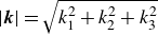 $|\boldsymbol{k}|=\sqrt {k_{1}^{2}+k_{2}^{2}+k_{3}^{2}}$
. Additionally,
$|\boldsymbol{k}|=\sqrt {k_{1}^{2}+k_{2}^{2}+k_{3}^{2}}$
. Additionally, $\omega$
is the non-dimensional angular frequency, which is related to the dimensional frequency
$\omega$
is the non-dimensional angular frequency, which is related to the dimensional frequency $\tilde {\omega }$
by
$\tilde {\omega }$
by $\omega = 2\pi \tilde {\omega } \tilde {L} / \tilde {u}_{\infty }$
.
$\omega = 2\pi \tilde {\omega } \tilde {L} / \tilde {u}_{\infty }$
.
There are four distinct modes of fluctuation in a uniform compressible stream: fast and slow acoustic waves, entropy waves, and vorticity waves (Zhong Reference Zhong2001). Their corresponding eigenvectors are given by
 \begin{align} \hat {\boldsymbol{\varphi }}_{\infty ,{f/s}} &= \epsilon _a \left (M_{\infty }^2, \pm \frac {k_1}{|\boldsymbol{k}|} M_{\infty }, \pm \frac {k_2}{|\boldsymbol{k}|} M_{\infty }, \pm \frac {k_3}{|\boldsymbol{k}|} M_{\infty }, (\gamma -1) M_{\infty }^2\right )^{{T}}, \\[-12pt] \nonumber \end{align}
 \begin{align} \hat {\boldsymbol{\varphi }}_{\infty ,{e}} &= \epsilon _e (1, 0, 0, 0, -1)^{{T}}, \\[-12pt] \nonumber \end{align}
 \begin{align} \hat {\boldsymbol{\varphi }}_{\infty ,{v}} &= \epsilon _v \left (0, -\frac {k_3}{\sqrt {k_1^2 + k_3^2}}, 0, \frac {k_1}{\sqrt {k_1^2 + k_3^2}}, 0\right )^{{T}}, \\[10pt] \nonumber \end{align}
where the subscripts $(\boldsymbol{\cdot })_{{f}}$
,
$(\boldsymbol{\cdot })_{{f}}$
, $(\boldsymbol{\cdot })_{{s}}$
,
$(\boldsymbol{\cdot })_{{s}}$
, $(\boldsymbol{\cdot })_{{e}}$
and
$(\boldsymbol{\cdot })_{{e}}$
and $(\boldsymbol{\cdot })_{{v}}$
denote fast acoustic, slow acoustic, entropy and vorticity waves, respectively, and
$(\boldsymbol{\cdot })_{{v}}$
denote fast acoustic, slow acoustic, entropy and vorticity waves, respectively, and $\epsilon$
represents the amplitude parameter. For the acoustic modes, the plus (
$\epsilon$
represents the amplitude parameter. For the acoustic modes, the plus ( $+$
) and minus (
$+$
) and minus ( $-$
) signs correspond to fast and slow waves, respectively. The vorticity mode eigenfunction is not unique; the specific form in (3.9c
) adopted here is adapted from Schrader et al. (Reference Schrader, Brandt, Mavriplis and Henningson2010), with the assumption
$-$
) signs correspond to fast and slow waves, respectively. The vorticity mode eigenfunction is not unique; the specific form in (3.9c
) adopted here is adapted from Schrader et al. (Reference Schrader, Brandt, Mavriplis and Henningson2010), with the assumption $k_2 = 0$
. The corresponding dispersion relations are given by
$k_2 = 0$
. The corresponding dispersion relations are given by
 \begin{align} \omega &= k_1 \pm \frac {|\boldsymbol{k}|}{M_{\infty }} \quad\quad \text{for acoustic waves,} \\[-12pt] \nonumber \end{align}
 \begin{align} \omega &= k_1 \quad\qquad\qquad \text{for entropy and vorticity waves.} \\[10pt] \nonumber \end{align}
The amplitudes $\epsilon _a$
,
$\epsilon _a$
, $\epsilon _e$
and
$\epsilon _e$
and $\epsilon _v$
are selected to ensure that the disturbances have equal energy norm, based on the Chu energy
$\epsilon _v$
are selected to ensure that the disturbances have equal energy norm, based on the Chu energy $E_{{Chu}}$
(Chu Reference Chu1965), which is defined as
$E_{{Chu}}$
(Chu Reference Chu1965), which is defined as
 \begin{align} E_{{Chu}}=\frac {1}{2} \left [\bar {\rho } \big(u^{\prime 2} + v^{\prime 2} + w^{\prime 2} \big)+\frac {\bar {T}}{\bar {\rho } \gamma M^2}\left (\rho ^{\prime }\right )^2+\frac {\bar {\rho }}{(\gamma -1) \gamma M^2 \bar {T}}\left (T^{\prime }\right )^2\right ], \end{align}
where $\bar {(\boldsymbol{\cdot })}$
and
$\bar {(\boldsymbol{\cdot })}$
and $(\boldsymbol{\cdot })^{\prime }$
represent base flow quantities and perturbation quantities, respectively. By evaluating the Chu energy corresponding to each disturbance mode in (3.9), the amplitude parameters are normalised to satisfy
$(\boldsymbol{\cdot })^{\prime }$
represent base flow quantities and perturbation quantities, respectively. By evaluating the Chu energy corresponding to each disturbance mode in (3.9), the amplitude parameters are normalised to satisfy
 \begin{align} \epsilon _a = \big(\sqrt {0.8} M_{\infty }^2 \big) \epsilon _e = (\sqrt {2} M_{\infty }) \epsilon _v = \epsilon _0, \end{align}
where $\epsilon _0$
is a reference amplitude, set to unity (
$\epsilon _0$
is a reference amplitude, set to unity ( $\epsilon _0 = 1$
) in the present study.
$\epsilon _0 = 1$
) in the present study.
This study focuses only on slow acoustic, entropy and vorticity waves. Fast acoustic waves are excluded as they are not the dominant disturbance modes in typical wind-tunnel or free-flight environments. For the remaining modes – slow acoustic, entropy and vorticity waves – the amplitude $\epsilon$
is assumed to be independent of the frequency
$\epsilon$
is assumed to be independent of the frequency $\tilde {\omega }$
. For slow acoustic waves, it is shown in § 4.2.5 that incorporating frequency-dependent amplitudes derived from wind-tunnel power spectral density (PSD) data does not alter the conclusions of this work. For entropy and vorticity waves, the constant amplitude assumption is adopted due to the lack of available PSD data.
$\tilde {\omega }$
. For slow acoustic waves, it is shown in § 4.2.5 that incorporating frequency-dependent amplitudes derived from wind-tunnel power spectral density (PSD) data does not alter the conclusions of this work. For entropy and vorticity waves, the constant amplitude assumption is adopted due to the lack of available PSD data.
3.3. Linearised N–S equations solver
We consider the dynamics of small-amplitude perturbations $\boldsymbol{Q}^{\prime }$
superimposed on the two-dimensional steady base flow
$\boldsymbol{Q}^{\prime }$
superimposed on the two-dimensional steady base flow $\bar {\boldsymbol{Q}}$
. The linearised governing equation of the perturbations, with an external forcing
$\bar {\boldsymbol{Q}}$
. The linearised governing equation of the perturbations, with an external forcing $\boldsymbol{f}^{\prime }$
, can be written in operator form as
$\boldsymbol{f}^{\prime }$
, can be written in operator form as
 \begin{align} \frac {\partial\kern-1pt\boldsymbol{Q}^{\prime }}{\partial t} = \mathcal{A}\kern-1pt\boldsymbol{Q}^{\prime } + \mathcal{B}\boldsymbol{f}^{\prime }, \end{align}
where $\mathcal{A}$
is the linearised N–S operator evaluated from the base flow. The derivation and the full continuous form of
$\mathcal{A}$
is the linearised N–S operator evaluated from the base flow. The derivation and the full continuous form of $\mathcal{A}$
can be found from Rolandi et al. (Reference Rolandi, Ribeiro, Yeh and Taira2024). The operator
$\mathcal{A}$
can be found from Rolandi et al. (Reference Rolandi, Ribeiro, Yeh and Taira2024). The operator $\mathcal{B}$
localises the forcing to a prescribed region, which is defined such that
$\mathcal{B}$
localises the forcing to a prescribed region, which is defined such that
 \begin{align} (\mathcal{B}\boldsymbol{f}^{\prime })(\boldsymbol{x}) = \begin{cases} \boldsymbol{f}^{\prime }(\boldsymbol{x}) & \text{for } \boldsymbol{x} \in \varOmega _{\kern-1pt f}, \\ \boldsymbol{0} & \text{for } \boldsymbol{x} \notin \varOmega _{\kern-1pt f}, \end{cases} \end{align}
where $\varOmega _{\kern-1pt f}$
denotes the forcing region and
$\varOmega _{\kern-1pt f}$
denotes the forcing region and $\boldsymbol{x} = (x,y,z)$
.
$\boldsymbol{x} = (x,y,z)$
.
Assuming the forcing and response are harmonic in time and the spanwise direction, we introduce the ansatz
 \begin{align} \begin{aligned} \boldsymbol{f}^{\prime }(\boldsymbol x, t) & =\kern2pt\hat {\boldsymbol{\kern-2pt f}}(x, y) \exp \left (\mathrm{i} k_3 z-\mathrm{i} \omega t\right ), \\ \boldsymbol{Q}^{\prime }(\boldsymbol x, t) & =\kern2pt \hat {\boldsymbol{\kern-2pt Q}}(x, y) \exp \left (\mathrm{i} k_3 z-\mathrm{i} \omega t\right ). \end{aligned} \end{align}
Substituting the harmonic ansatz (3.15) into (3.13) yields the linear system that relates the forcing and the response:
 \begin{align} \kern2pt \hat {\boldsymbol{\kern-2pt Q}}=\mathcal{R} \mathcal{B}\kern2pt\hat {\boldsymbol{\kern-2pt f}}, \end{align}
where $\mathcal{R} = (-\mathrm{i}\omega \mathcal{I}-\mathcal{A} )^{-1}$
is called the resolvent and
$\mathcal{R} = (-\mathrm{i}\omega \mathcal{I}-\mathcal{A} )^{-1}$
is called the resolvent and $\mathcal{I}$
is the identity operator.
$\mathcal{I}$
is the identity operator.
To investigate the receptivity to free stream disturbances, we employ an internal Dirichlet boundary condition to constrain the solution within a prescribed forcing region $\varOmega _{\kern-1pt f}$
. The objective is to enforce the planar wave solution given in § 3.2 inside
$\varOmega _{\kern-1pt f}$
. The objective is to enforce the planar wave solution given in § 3.2 inside $\varOmega _{\kern-1pt f}$
, i.e.
$\varOmega _{\kern-1pt f}$
, i.e.
 \begin{align} \boldsymbol Q^{\prime }(\boldsymbol x,t)=\boldsymbol{J}\boldsymbol \varphi ^{\prime }(\boldsymbol x,t) \quad \text{for } \boldsymbol{x} \in \varOmega _{\kern-1pt f}, \end{align}
where $\boldsymbol{J}$
is defined such that
$\boldsymbol{J}$
is defined such that $\boldsymbol{Q}^{\prime } = \boldsymbol{J}\boldsymbol{\varphi }^{\prime }$
; further details can be found from Rolandi et al. (Reference Rolandi, Ribeiro, Yeh and Taira2024). Since plane waves are harmonic in every direction and in time, we can substitute (3.17) into (3.13). Following the same derivation as before, we obtain
$\boldsymbol{Q}^{\prime } = \boldsymbol{J}\boldsymbol{\varphi }^{\prime }$
; further details can be found from Rolandi et al. (Reference Rolandi, Ribeiro, Yeh and Taira2024). Since plane waves are harmonic in every direction and in time, we can substitute (3.17) into (3.13). Following the same derivation as before, we obtain
 \begin{align} \boldsymbol{J} \hat {\boldsymbol \varphi }(x,y) = \left (-\mathrm{i}\omega \mathcal{I}-\mathcal{A}\right )^{-1} \mathcal{B}\kern2pt\hat {\boldsymbol{\kern-2pt f}}(x,y) = \left (-\mathrm{i}\omega \mathcal{I}-\mathcal{A}\right )^{-1} \kern2pt\hat {\boldsymbol{\kern-2pt f}}(x,y)\quad\text{ for } (x,y) \in \varOmega _{\kern-1pt f}. \end{align}
For numerical implementation, the operator $\mathcal{A}$
can be replaced by a zero operator within the forcing region, i.e.
$\mathcal{A}$
can be replaced by a zero operator within the forcing region, i.e.
 \begin{align} \mathcal{A}(x,y) = 0 \quad \text{for } (x,y) \in \varOmega _{\kern-1pt f}. \end{align}
Hence, (3.18) can be simplified as follows:
 \begin{align} \kern2pt\hat {\boldsymbol{\kern-2pt f}}(x,y) = -\mathrm{i}\omega \boldsymbol{J} \hat {\boldsymbol{\varphi }}_\infty \exp (\mathrm{i}k_1 x + \mathrm{i}k_2 y), \end{align}
where $\hat {\boldsymbol{\varphi }}_\infty$
can be any disturbance mode given in (3.9). This formulation generates the desired disturbance at the specified location, allowing it to propagate downstream and interact with the shock and boundary layer.
$\hat {\boldsymbol{\varphi }}_\infty$
can be any disturbance mode given in (3.9). This formulation generates the desired disturbance at the specified location, allowing it to propagate downstream and interact with the shock and boundary layer.
The linear system is discretised using the finite-volume method. Upon spatial discretisation, the operators $\mathcal{A}$
,
$\mathcal{A}$
, $\mathcal{I}$
,
$\mathcal{I}$
, $\mathcal{R}$
and
$\mathcal{R}$
and $\mathcal{B}$
are approximated by matrices
$\mathcal{B}$
are approximated by matrices $\boldsymbol{A}$
,
$\boldsymbol{A}$
, $\boldsymbol{I}$
,
$\boldsymbol{I}$
, $\boldsymbol{R}$
and
$\boldsymbol{R}$
and $\boldsymbol{B}$
, respectively, i.e.
$\boldsymbol{B}$
, respectively, i.e.
 \begin{align} \kern2pt \hat {\boldsymbol{\kern-2pt Q}}=\boldsymbol{RB}\kern2pt\hat {\boldsymbol{\kern-2pt f}}, \end{align}
where $\boldsymbol{R} = (-\mathrm{i}\omega \boldsymbol{I}-\boldsymbol{A} )^{-1}$
and
$\boldsymbol{R} = (-\mathrm{i}\omega \boldsymbol{I}-\boldsymbol{A} )^{-1}$
and $\boldsymbol{I}$
is the identity matrix. For the operator
$\boldsymbol{I}$
is the identity matrix. For the operator $\mathcal{A}$
, the inviscid fluxes are discretised via the modified Steger–Warming scheme (MacCormack Reference MacCormack2014). To achieve high-order spatial accuracy, variables at cell interfaces are reconstructed using a third-order MUSCL scheme. The viscous fluxes are discretised using second-order central differences. More details about the discretisation of
$\mathcal{A}$
, the inviscid fluxes are discretised via the modified Steger–Warming scheme (MacCormack Reference MacCormack2014). To achieve high-order spatial accuracy, variables at cell interfaces are reconstructed using a third-order MUSCL scheme. The viscous fluxes are discretised using second-order central differences. More details about the discretisation of $\mathcal{A}$
are provided in Appendix C. The matrix
$\mathcal{A}$
are provided in Appendix C. The matrix $\boldsymbol{B}$
is a sparse binary matrix with a size of
$\boldsymbol{B}$
is a sparse binary matrix with a size of $N\times N$
, where
$N\times N$
, where $N =N_{{cell}} \times m$
. Here,
$N =N_{{cell}} \times m$
. Here, $N_{{cell}}$
is the total number of cells and
$N_{{cell}}$
is the total number of cells and $m=5$
is the number of variables. The diagonal blocks are
$m=5$
is the number of variables. The diagonal blocks are $m \times m$
identity matrices for grid points within
$m \times m$
identity matrices for grid points within ${\varOmega }_f$
, and zero matrices otherwise. The resulting linear system is solved via lower-upper decomposition using the MUMPS package (Amestoy et al. Reference Amestoy, Duff, Koster and L’Excellent2001).
${\varOmega }_f$
, and zero matrices otherwise. The resulting linear system is solved via lower-upper decomposition using the MUMPS package (Amestoy et al. Reference Amestoy, Duff, Koster and L’Excellent2001).
For all $\tilde {R}_n$
, we consider 37 values of
$\tilde {R}_n$
, we consider 37 values of $\tilde {\omega }$
ranging from 1 to 200 kHz and 30 values of
$\tilde {\omega }$
ranging from 1 to 200 kHz and 30 values of $k_3$
ranging from 0 to 10. The forcing region is positioned upstream of the bow shock, specifically along the grid line
$k_3$
ranging from 0 to 10. The forcing region is positioned upstream of the bow shock, specifically along the grid line $j = 631$
(see figure 1). This placement ensures that a uniform plane wave impinges on the bow shock. In this work, we define the receptivity gain, denoted as
$j = 631$
(see figure 1). This placement ensures that a uniform plane wave impinges on the bow shock. In this work, we define the receptivity gain, denoted as $G$
, as the Chu energy (Chu Reference Chu1965) integrated over the output region. The output region covers the entire boundary layer on the flat plate (i.e. at each streamwise station
$G$
, as the Chu energy (Chu Reference Chu1965) integrated over the output region. The output region covers the entire boundary layer on the flat plate (i.e. at each streamwise station $x$
, the integration of Chu energy extends from the wall to the local boundary layer thickness). Subscripts
$x$
, the integration of Chu energy extends from the wall to the local boundary layer thickness). Subscripts $(\boldsymbol{\cdot })_{a}$
,
$(\boldsymbol{\cdot })_{a}$
, $(\boldsymbol{\cdot })_{e}$
and
$(\boldsymbol{\cdot })_{e}$
and $(\boldsymbol{\cdot })_{v}$
are used to distinguish the receptivity gains for different disturbance waves. For example, the receptivity gain corresponding to slow acoustic waves is denoted by
$(\boldsymbol{\cdot })_{v}$
are used to distinguish the receptivity gains for different disturbance waves. For example, the receptivity gain corresponding to slow acoustic waves is denoted by $G_{a}$
.
$G_{a}$
.
The framework is equivalent to solving the LNSE in a time-dependent manner, where disturbances, such as slow acoustic waves, are introduced from the free stream. The verification of the framework is provided in Appendix B. A practical advantage of the present framework is that the computational cost is insensitive to the smallest grid spacing, which would otherwise impose a restrictive CFL constraint when the nose radius is small.
3.4. Resolvent analysis
In addition to the LNSE, resolvent analysis is also performed to identify the optimal forcing and response modes. The following input locations are considered.
-
(i) The same upstream free stream region used for the free stream physical forcing cases in § 3.3.
-
(ii) A wall-normal line at $x=0$
extending from the wall to the inner edge of the bow shock.
$x=0$
extending from the wall to the inner edge of the bow shock. -
(iii) A wall-normal line at station
$\phi =30^\circ$
extending from the wall to the inner edge of the bow shock. The angle
$\phi$
is measured from the stagnation line and
$\phi =90^\circ$
is equivalent to
$x=0$
.


The first two forcing regions correspond to forcing locations 1 and 2 in figure 1, and the last one is not shown for visual clarity. The choice of these input locations is to investigate the influence of nose-tip receptivity on downstream perturbation development, as will be discussed in § 4.4. The output region remains unchanged, i.e. the entire boundary layer on the flat plate.
We define the input–output relation starting from the linear system given by (3.16). An additional restriction matrix $\boldsymbol{C}$
is introduced to extract the state vector within the region of interest (output domain), such that the output response
$\boldsymbol{C}$
is introduced to extract the state vector within the region of interest (output domain), such that the output response $\kern1pt \hat {\boldsymbol{\kern-1pt U}}$
is given by
$\kern1pt \hat {\boldsymbol{\kern-1pt U}}$
is given by
 \begin{align} \kern1pt \hat {\boldsymbol{\kern-1pt U}} = \boldsymbol{C} \hat {\boldsymbol{\kern-2pt Q}} = \boldsymbol{CRB} \kern2pt\hat {\boldsymbol{\kern-2pt f}}, \end{align}
where $\boldsymbol{C}$
is also a sparse binary matrix, similar in nature to
$\boldsymbol{C}$
is also a sparse binary matrix, similar in nature to $\boldsymbol{B}$
. The diagonal blocks are
$\boldsymbol{B}$
. The diagonal blocks are $m \times m$
identity matrices for grid points in the output region and zero matrices otherwise. Resolvent analysis identifies the optimal forcing and the corresponding optimal response as the pair that maximises the energy gain
$m \times m$
identity matrices for grid points in the output region and zero matrices otherwise. Resolvent analysis identifies the optimal forcing and the corresponding optimal response as the pair that maximises the energy gain $G_o$
. This gain is defined as the ratio of the output energy to the input energy:
$G_o$
. This gain is defined as the ratio of the output energy to the input energy:
 \begin{align} G_o(\omega ,k_3) =\max _{\kern2pt \hat {\boldsymbol{\kern-2pt f}}\neq \boldsymbol 0} \frac {\|\hat {\boldsymbol U}\|_{E}}{\|\,\boldsymbol{B} \kern2pt \hat {\boldsymbol{\kern-2pt f}}\,\|_{E}}. \end{align}
The energy norms are also defined based on the Chu energy (Chu Reference Chu1965), which can be expressed using a positive-definite weight matrix $\boldsymbol{M}$
:
$\boldsymbol{M}$
:
 \begin{align} \|\boldsymbol{U}\|_{E}^{2} = \boldsymbol{U}^{*}\,\boldsymbol{M}\,\boldsymbol{U}, \end{align}
where $(\boldsymbol{\cdot })^{*}$
denotes the conjugate transpose. The detailed expression for
$(\boldsymbol{\cdot })^{*}$
denotes the conjugate transpose. The detailed expression for $\boldsymbol{M}$
is provided by Bugeat et al. (Reference Bugeat, Chassaing, Robinet and Sagaut2019). Physically, the optimal forcing now represents the specific input disturbance that undergoes the strongest linear amplification in terms of the Chu energy from the input region to the output region. The optimisation problem (3.23) can be converted to an eigenvalue problem as
$\boldsymbol{M}$
is provided by Bugeat et al. (Reference Bugeat, Chassaing, Robinet and Sagaut2019). Physically, the optimal forcing now represents the specific input disturbance that undergoes the strongest linear amplification in terms of the Chu energy from the input region to the output region. The optimisation problem (3.23) can be converted to an eigenvalue problem as
 \begin{align} \boldsymbol{B^{*}}\,\boldsymbol{R^{*}}\,\boldsymbol{C^{*}}\,\boldsymbol M\,\boldsymbol{C}\,\boldsymbol{R}\,\boldsymbol{B}\, \kern2pt \hat {\boldsymbol{\kern-2pt f}} = G_o^{2}\,\kern2pt \hat {\boldsymbol{\kern-2pt f}}. \end{align}
The verification of the conventional resolvent analysis code can be found from Hao et al. (Reference Hao, Cao, Guo and Wen2023). It is important to note that the optimal gain $G_o$
is conceptually different from the receptivity gain
$G_o$
is conceptually different from the receptivity gain $G$
and, therefore, the two values are not comparable.
$G$
and, therefore, the two values are not comparable.
4. Results and discussion
This section presents the results of the study. Section 4.1 presents results for the base flow. Section 4.2 reports the results for slow acoustic disturbances at zero angle of incidence. Section 4.3 reports the results for entropy and vorticity disturbances. Section 4.4 shows the results for resolvent analysis. Section 4.5 examines the effects of a non-zero angle of incidence of disturbance for slow acoustic disturbances.
4.1. Base flow features
Figure 2 presents the evolution of the boundary-layer thickness $\delta _h$
and entropy-layer thickness
$\delta _h$
and entropy-layer thickness $\delta _s$
. Following Paredes et al. (Reference Paredes, Choudhari, Li, Jewell and Kimmel2019a
) and Scholten et al. (Reference Scholten, Goparaju, Gaitonde, Paredes, Choudhari and Li2022), the boundary-layer edge is defined as the location where the local total enthalpy
$\delta _s$
. Following Paredes et al. (Reference Paredes, Choudhari, Li, Jewell and Kimmel2019a
) and Scholten et al. (Reference Scholten, Goparaju, Gaitonde, Paredes, Choudhari and Li2022), the boundary-layer edge is defined as the location where the local total enthalpy $\tilde {h}_t$
reaches 99.5 % of its free stream value, where
$\tilde {h}_t$
reaches 99.5 % of its free stream value, where $\tilde {h}_t = \tilde {c}_p \tilde {T} + (\tilde {u}^2 + \tilde {v}^2)/2$
. The specific heat at constant pressure
$\tilde {h}_t = \tilde {c}_p \tilde {T} + (\tilde {u}^2 + \tilde {v}^2)/2$
. The specific heat at constant pressure $\tilde {c}_p$
is
$\tilde {c}_p$
is $1004\, \mathrm{J\,(kg\,K)}^{-1}$
. The entropy-layer edge is where the local entropy increment
$1004\, \mathrm{J\,(kg\,K)}^{-1}$
. The entropy-layer edge is where the local entropy increment $\Delta \tilde {S}$
is 25 % of that at the wall. The local entropy increment is given as
$\Delta \tilde {S}$
is 25 % of that at the wall. The local entropy increment is given as $\Delta \tilde {S}=\tilde {c}_p \ln (\tilde {T} / \tilde {T}_\infty )-\tilde{\mathscr{R}} \ln (\tilde {p} / \tilde {p}_{\infty} )$
, where
$\Delta \tilde {S}=\tilde {c}_p \ln (\tilde {T} / \tilde {T}_\infty )-\tilde{\mathscr{R}} \ln (\tilde {p} / \tilde {p}_{\infty} )$
, where $\tilde{\mathscr{R}} = 287\,\mathrm{J\,(kg\,K)}^{-1}$
is the specific gas constant for air.
$\tilde{\mathscr{R}} = 287\,\mathrm{J\,(kg\,K)}^{-1}$
is the specific gas constant for air.
Streamwise evolution of (a) boundary-layer thickness and (b) entropy-layer thickness.

Near the leading edge, the boundary-layer thickness $\delta _h$
exhibits a non-monotonic variation, including a local reduction. This behaviour is mainly associated with the specific boundary-layer edge definition adopted in the present study. Further downstream, the effect of nose radius on the boundary-layer thickness becomes weak and the differences in
$\delta _h$
exhibits a non-monotonic variation, including a local reduction. This behaviour is mainly associated with the specific boundary-layer edge definition adopted in the present study. Further downstream, the effect of nose radius on the boundary-layer thickness becomes weak and the differences in $\delta _h$
among the cases are small. Unlike the boundary layer, the entropy layer thickens significantly with increasing
$\delta _h$
among the cases are small. Unlike the boundary layer, the entropy layer thickens significantly with increasing $\tilde {R}_n$
. As the flow progresses downstream, the entropy-layer thickness
$\tilde {R}_n$
. As the flow progresses downstream, the entropy-layer thickness $\delta _s$
approaches a nearly constant value and the streamwise distance required to reach this state increases with
$\delta _s$
approaches a nearly constant value and the streamwise distance required to reach this state increases with $\tilde {R}_n$
. Although the growth of the boundary layer suggests that it would eventually swallow the entropy layer far downstream, this is not observed within the current computational domain for any of the cases. Hence, the modal instabilities are expected to be stabilised as the nose radius increases.
$\tilde {R}_n$
. Although the growth of the boundary layer suggests that it would eventually swallow the entropy layer far downstream, this is not observed within the current computational domain for any of the cases. Hence, the modal instabilities are expected to be stabilised as the nose radius increases.
4.2. Response to free stream slow acoustic waves at zero angle of incidence
This section investigates the response of the boundary layer to free stream slow acoustic waves at zero angle of incidence. Figure 3 shows the contours of $G_a$
in
$G_a$
in $k_3{-}\tilde {\omega }$
space for different
$k_3{-}\tilde {\omega }$
space for different $\tilde {R}_n$
. These contours have several local peaks, depending on
$\tilde {R}_n$
. These contours have several local peaks, depending on $\tilde {R}_n$
. These peaks are associated with the oblique first-mode instability, streamwise streaks or entropy layer instability.
$\tilde {R}_n$
. These peaks are associated with the oblique first-mode instability, streamwise streaks or entropy layer instability.
Contours of $G_a$
in the boundary layer on the flat plate in response to free stream slow acoustic waves with zero angle of incidence for cases (a)
$G_a$
in the boundary layer on the flat plate in response to free stream slow acoustic waves with zero angle of incidence for cases (a) ${\mathrm{R}01}_{A}$
, (b)
${\mathrm{R}01}_{A}$
, (b) ${\mathrm{R}02}_{A}$
, (c)
${\mathrm{R}02}_{A}$
, (c) ${\mathrm{R}05}_{A}$
, (d)
${\mathrm{R}05}_{A}$
, (d) ${\mathrm{R}07}_{A}$
, (e)
${\mathrm{R}07}_{A}$
, (e) ${\mathrm{R}1}_{A}$
and (f)
${\mathrm{R}1}_{A}$
and (f) ${\mathrm{R}2}_{A}$
.
${\mathrm{R}2}_{A}$
.

Figure 3. Long description
Panel A: A heat map showing the boundary-layer transition with the oblique first mode highlighted. The x-axis represents k3 values ranging from 0 to 10, and the y-axis represents omega values ranging from 10^0 to 10^2 kHz. The color scale on the right indicates the magnitude of the values, with red representing higher values and blue representing lower values. Panel B: A heat map showing the boundary-layer transition with streaks highlighted. The x-axis represents k3 values ranging from 0 to 10, and the y-axis represents omega values ranging from 10^0 to 10^2 kHz. The color scale on the right indicates the magnitude of the values, with red representing higher values and blue representing lower values. Panel C: A heat map showing the boundary-layer transition with entropy layer instability highlighted. The x-axis represents k3 values ranging from 0 to 10, and the y-axis represents omega values ranging from 10^0 to 10^2 kHz. The color scale on the right indicates the magnitude of the values, with red representing higher values and blue representing lower values. Panel D: A heat map showing the boundary-layer transition. The x-axis represents k3 values ranging from 0 to 10, and the y-axis represents omega values ranging from 10^0 to 10^2 kHz. The color scale on the right indicates the magnitude of the values, with red representing higher values and blue representing lower values. Panel E: A heat map showing the boundary-layer transition. The x-axis represents k3 values ranging from 0 to 10, and the y-axis represents omega values ranging from 10^0 to 10^2 kHz. The color scale on the right indicates the magnitude of the values, with red representing higher values and blue representing lower values. Panel F: A heat map showing the boundary-layer transition with entropy layer instability highlighted. The x-axis represents k3 values ranging from 0 to 10, and the y-axis represents omega values ranging from 10^0 to 10^2 kHz. The color scale on the right indicates the magnitude of the values, with red representing higher values and blue representing lower values.
(a) Contour of $u^{\prime }_{r}$
for case
$u^{\prime }_{r}$
for case ${\mathrm{R}01}_{A}$
. The dashed and solid lines represent the edges of the boundary layer and entropy layer, respectively. (b) Comparison of the spatial amplification rates
${\mathrm{R}01}_{A}$
. The dashed and solid lines represent the edges of the boundary layer and entropy layer, respectively. (b) Comparison of the spatial amplification rates $-{\alpha }_i$
obtained from classical modal LST and LNSE for case
$-{\alpha }_i$
obtained from classical modal LST and LNSE for case ${\mathrm{R}01}_{A}$
. Both plots are for
${\mathrm{R}01}_{A}$
. Both plots are for $\tilde {\omega } = 16.351$
kHz and
$\tilde {\omega } = 16.351$
kHz and $k_3 = 0.6$
.
$k_3 = 0.6$
.

4.2.1. Oblique first mode
The local peaks at approximately $k_3 = 0.6$
and
$k_3 = 0.6$
and $\tilde {\omega } = 16.351\,\mathrm{kHz}$
are associated with the oblique first mode. Figure 4(a) plots the contour of
$\tilde {\omega } = 16.351\,\mathrm{kHz}$
are associated with the oblique first mode. Figure 4(a) plots the contour of $u^{\prime }_r$
at the same
$u^{\prime }_r$
at the same $\tilde {\omega }$
and
$\tilde {\omega }$
and $k_3$
for case
$k_3$
for case ${\mathrm{R}01}_{A}$
, where
${\mathrm{R}01}_{A}$
, where $(\boldsymbol{\cdot })^{\prime }_r$
refers to the real part of the perturbation. The dashed and solid lines represent the edges of the boundary layer and entropy layer, respectively. This single-cell structure is a clear signature of the first mode, which amplifies as it progresses. Figure 4(b) compares the spatial amplification rates,
$(\boldsymbol{\cdot })^{\prime }_r$
refers to the real part of the perturbation. The dashed and solid lines represent the edges of the boundary layer and entropy layer, respectively. This single-cell structure is a clear signature of the first mode, which amplifies as it progresses. Figure 4(b) compares the spatial amplification rates, $-{\alpha }_i$
, obtained from classical modal LST (Guo, Hao & Wen Reference Guo, Hao and Wen2023) with those from LNSE. The computational domain is extended to 650 mm to facilitate comparison. For the LNSE results,
$-{\alpha }_i$
, obtained from classical modal LST (Guo, Hao & Wen Reference Guo, Hao and Wen2023) with those from LNSE. The computational domain is extended to 650 mm to facilitate comparison. For the LNSE results, $-{\alpha }_i$
is calculated as
$-{\alpha }_i$
is calculated as $-{\alpha }_i=({1}/ {|p^\prime _{w\textit{all}}|}) ( {\partial |p^\prime _{w\textit{all}}|}/{\partial x})$
, where
$-{\alpha }_i=({1}/ {|p^\prime _{w\textit{all}}|}) ( {\partial |p^\prime _{w\textit{all}}|}/{\partial x})$
, where $(\boldsymbol{\cdot })^\prime _{w\textit{all}}$
and
$(\boldsymbol{\cdot })^\prime _{w\textit{all}}$
and $|(\boldsymbol{\cdot })^\prime |$
refer to the perturbation at the wall and perturbation magnitude, respectively. For LST results, two grid resolutions are used to ensure grid independence. The neutral point is located at
$|(\boldsymbol{\cdot })^\prime |$
refer to the perturbation at the wall and perturbation magnitude, respectively. For LST results, two grid resolutions are used to ensure grid independence. The neutral point is located at $x \approx 35$
. For
$x \approx 35$
. For $x\lt 500$
, the agreement is poor due to non-parallel effects and non-modal effects. In the downstream region (
$x\lt 500$
, the agreement is poor due to non-parallel effects and non-modal effects. In the downstream region ( $x\gt 500$
), where the flow becomes similar to that over a flat plate, the agreement improves, indicating that the growth is fully dominated by modal instability. Nevertheless, the LST can still accurately predict the perturbation profiles within the normal computational domain (
$x\gt 500$
), where the flow becomes similar to that over a flat plate, the agreement improves, indicating that the growth is fully dominated by modal instability. Nevertheless, the LST can still accurately predict the perturbation profiles within the normal computational domain ( $x \leqslant 200$
). Figure 5 presents the eigenspectra of the complex phase velocity computed using the LST for different cases at
$x \leqslant 200$
). Figure 5 presents the eigenspectra of the complex phase velocity computed using the LST for different cases at $x=100$
,
$x=100$
, $150$
and
$150$
and $200$
, for
$200$
, for $\tilde {\omega } = 16.351$
kHz and
$\tilde {\omega } = 16.351$
kHz and $k_3 = 0.6$
. At each location, only one discrete mode is unstable, which corresponds to the first mode. In figure 6, we plot the eigenfunctions of
$k_3 = 0.6$
. At each location, only one discrete mode is unstable, which corresponds to the first mode. In figure 6, we plot the eigenfunctions of $\left |u^{\prime }\right |$
,
$\left |u^{\prime }\right |$
, $\left |v^{\prime }\right |$
and
$\left |v^{\prime }\right |$
and $\left |w^{\prime }\right |$
for these unstable discrete modes. Within the boundary layer, the eigenfunctions agree well with the velocity perturbation profiles obtained from the LNSE. The structure of
$\left |w^{\prime }\right |$
for these unstable discrete modes. Within the boundary layer, the eigenfunctions agree well with the velocity perturbation profiles obtained from the LNSE. The structure of $u^{\prime }_r$
, and the close agreement between the LNSE and LST results confirm that the peaks at
$u^{\prime }_r$
, and the close agreement between the LNSE and LST results confirm that the peaks at $\tilde {\omega } = 16.351\,\mathrm{kHz}$
and
$\tilde {\omega } = 16.351\,\mathrm{kHz}$
and $k_3 = 0.6$
in figure 3 are attributed to the oblique first mode. The corresponding
$k_3 = 0.6$
in figure 3 are attributed to the oblique first mode. The corresponding $G_a$
value decreases as
$G_a$
value decreases as $\tilde {R}_n$
increases, a trend attributed to the stabilising effect of the nose on modal instability.
$\tilde {R}_n$
increases, a trend attributed to the stabilising effect of the nose on modal instability.
Eigenspectra of the complex phase velocity for (a) case ${\mathrm{R}01}_{A}$
at
${\mathrm{R}01}_{A}$
at $x = 100$
, (b) case
$x = 100$
, (b) case ${\mathrm{R}07}_{A}$
at
${\mathrm{R}07}_{A}$
at $x = 150$
and (c) case
$x = 150$
and (c) case ${\mathrm{R}2}_{A}$
at
${\mathrm{R}2}_{A}$
at $x = 200$
. All plots are for
$x = 200$
. All plots are for $\tilde {\omega } = 16.351\,\mathrm{kHz}$
and
$\tilde {\omega } = 16.351\,\mathrm{kHz}$
and $k_3 = 0.6$
.
$k_3 = 0.6$
.

Profiles of velocity perturbations for $\tilde {\omega } = 16.351\,\mathrm{kHz}$
and
$\tilde {\omega } = 16.351\,\mathrm{kHz}$
and $k_3 = 0.6$
. The first, second and third columns are respectively for case
$k_3 = 0.6$
. The first, second and third columns are respectively for case ${\mathrm{R}01}_{A}$
at
${\mathrm{R}01}_{A}$
at $x = 100$
, case
$x = 100$
, case ${\mathrm{R}07}_{A}$
at
${\mathrm{R}07}_{A}$
at $x = 150$
and case
$x = 150$
and case ${\mathrm{R}2}_{A}$
at
${\mathrm{R}2}_{A}$
at $x = 200$
.
$x = 200$
.

Figure 6. Long description
The image contains nine line graphs arranged in a 3x3 grid, each representing velocity perturbation profiles for different cases and conditions. Panel A: The first column shows the profiles of |u’|/|u’|max for case at M = 4.5, case at M = 5.0, and case at M = 5.5. The x-axis represents |u’|/|u’|max, and the y-axis represents η. The graphs compare LNSE, LST, BL edge, and EL edge. Panel B: The second column shows the profiles of |v’|/|v’|max for the same cases. The x-axis represents |v’|/|v’|max, and the y-axis represents η. The graphs compare LNSE, LST, BL edge, and EL edge. Panel C: The third column shows the profiles of |w’|/|w’|max for the same cases. The x-axis represents |w’|/|w’|max, and the y-axis represents η. The graphs compare LNSE, LST, BL edge, and EL edge.
4.2.2. Streamwise streaks
The low-frequency peaks in figure 3 at approximately $\tilde {\omega } = 1\,\mathrm{kHz}$
and
$\tilde {\omega } = 1\,\mathrm{kHz}$
and $k_3 = 3.6$
, which first emerge when
$k_3 = 3.6$
, which first emerge when $\tilde {R}_n$
reaches 0.2 mm, correspond to streamwise streaks. The profiles of
$\tilde {R}_n$
reaches 0.2 mm, correspond to streamwise streaks. The profiles of $|u^{\prime }|$
,
$|u^{\prime }|$
, $|v^{\prime }|$
and
$|v^{\prime }|$
and $|w^{\prime }|$
at
$|w^{\prime }|$
at $x = 20$
are plotted in figure 7. It is evident that
$x = 20$
are plotted in figure 7. It is evident that $|u^{\prime }|$
is significantly larger than both
$|u^{\prime }|$
is significantly larger than both $|v^{\prime }|$
and
$|v^{\prime }|$
and $|w^{\prime }|$
, which is a signature of streaks. The peak of the
$|w^{\prime }|$
, which is a signature of streaks. The peak of the $|u^{\prime }|$
profile,
$|u^{\prime }|$
profile, $|u^{\prime }|_{max }$
, increases with
$|u^{\prime }|_{max }$
, increases with $\tilde {R}_n$
and is located near the boundary-layer edge. Notably, although the contour for case
$\tilde {R}_n$
and is located near the boundary-layer edge. Notably, although the contour for case ${\mathrm{R}01}_{A}$
lacks a distinct peak at
${\mathrm{R}01}_{A}$
lacks a distinct peak at $k_3 = 3.6$
, its corresponding velocity perturbation profiles exhibit a structure similar to that of the other cases.
$k_3 = 3.6$
, its corresponding velocity perturbation profiles exhibit a structure similar to that of the other cases.
Profiles of $|u^{\prime }|$
,
$|u^{\prime }|$
, $|v^{\prime }|$
and
$|v^{\prime }|$
and $|w^{\prime }|$
associated with
$|w^{\prime }|$
associated with $\tilde {\omega } = 1$
kHz and
$\tilde {\omega } = 1$
kHz and $k_3 = 3.6$
at
$k_3 = 3.6$
at $x = 20$
for cases (a)
$x = 20$
for cases (a) ${\mathrm{R}01}_{A}$
, (b)
${\mathrm{R}01}_{A}$
, (b) ${\mathrm{R}02}_{A}$
, (c)
${\mathrm{R}02}_{A}$
, (c) ${\mathrm{R}05}_{A}$
, (d)
${\mathrm{R}05}_{A}$
, (d) ${\mathrm{R}07}_{A}$
, (e)
${\mathrm{R}07}_{A}$
, (e) ${\mathrm{R}1}_{A}$
and (f)
${\mathrm{R}1}_{A}$
and (f) ${\mathrm{R}2}_{A}$
.
${\mathrm{R}2}_{A}$
.

(a) Evolution of $|u^{\prime }|_{{max}}$
along the streamwise direction. (b) Contour of
$|u^{\prime }|_{{max}}$
along the streamwise direction. (b) Contour of $u^{\prime }_{r}$
for case
$u^{\prime }_{r}$
for case ${\mathrm{R}2}_{A}$
. The dashed line represents the edge of the boundary layer. Both plots are for
${\mathrm{R}2}_{A}$
. The dashed line represents the edge of the boundary layer. Both plots are for $\tilde {\omega } = 1$
kHz and
$\tilde {\omega } = 1$
kHz and $k_3 = 3.6$
.
$k_3 = 3.6$
.

The strength of streaks can be quantified by $|u^{\prime }|_{max }$
. Figure 8(a) shows the streamwise evolution of
$|u^{\prime }|_{max }$
. Figure 8(a) shows the streamwise evolution of $|u^{\prime }|_{max }$
for all cases. Increasing
$|u^{\prime }|_{max }$
for all cases. Increasing $\tilde {R}_n$
enhances the streaks, corresponding to an increase in the receptivity gain in figure 3. Figure 8(b) presents the contour of
$\tilde {R}_n$
enhances the streaks, corresponding to an increase in the receptivity gain in figure 3. Figure 8(b) presents the contour of $u^{\prime }_r$
for case
$u^{\prime }_r$
for case $\mathrm{R2}_A$
, revealing the streaky structure of the disturbances. Note that
$\mathrm{R2}_A$
, revealing the streaky structure of the disturbances. Note that $u^{\prime }_r$
changes its sign near
$u^{\prime }_r$
changes its sign near $x = 100$
as a result of the non-zero frequency. The finite wavelength is due to the finite frequency of the free stream disturbance. Figure 9 demonstrates the effects of varying
$x = 100$
as a result of the non-zero frequency. The finite wavelength is due to the finite frequency of the free stream disturbance. Figure 9 demonstrates the effects of varying $\tilde {\omega }$
on the streaks for a given
$\tilde {\omega }$
on the streaks for a given $k_3$
and
$k_3$
and $\tilde {R}_n$
. Figure 9(a) shows that increasing the frequency promotes the saturation of the streaks, while reducing their maximum amplitude. However, reducing
$\tilde {R}_n$
. Figure 9(a) shows that increasing the frequency promotes the saturation of the streaks, while reducing their maximum amplitude. However, reducing $\tilde {\omega }$
below
$\tilde {\omega }$
below $1\,\mathrm{kHz}$
has a negligible impact on the evolution of
$1\,\mathrm{kHz}$
has a negligible impact on the evolution of $|u^\prime |_{{max}}$
, as the results for
$|u^\prime |_{{max}}$
, as the results for $\tilde {\omega } \leqslant 1\,\mathrm{kHz}$
nearly collapse. Figure 9(b) displays
$\tilde {\omega } \leqslant 1\,\mathrm{kHz}$
nearly collapse. Figure 9(b) displays $u^{\prime }_r$
contours for case
$u^{\prime }_r$
contours for case ${\mathrm{R}2}_{A}$
at
${\mathrm{R}2}_{A}$
at $\tilde {\omega } = 10\,\mathrm{kHz}$
and
$\tilde {\omega } = 10\,\mathrm{kHz}$
and $k_3 = 3.6$
. The streamwise wavelength of the streaks decreases as the frequency increases and the disturbances move away from the wall as they propagate downstream. The saturation point in figure 9(a) coincides with the location where the main structure of the disturbance begins to egress from the boundary layer. Notably, these high-frequency streaks closely resemble the elongated structures observed in various experiments. In particular, Hill et al. (Reference Hill, Oddo, Komives, Reeder, Borg and Jewell2022) reported that increasing the nose radius promotes the elongated, low-frequency disturbances observed in their experiments, which become dominant over the rope-like disturbances associated with the second mode at large nose radii. The frequency of the elongated structures ranged from 10 to 20 kHz, approximately five times lower than that of the rope-like structures in their study. Similar structures and a transition from rope-like to elongated forms were also reported by Kennedy et al. (Reference Kennedy, Jewell, Paredes and Laurence2022), albeit at higher frequencies.
$k_3 = 3.6$
. The streamwise wavelength of the streaks decreases as the frequency increases and the disturbances move away from the wall as they propagate downstream. The saturation point in figure 9(a) coincides with the location where the main structure of the disturbance begins to egress from the boundary layer. Notably, these high-frequency streaks closely resemble the elongated structures observed in various experiments. In particular, Hill et al. (Reference Hill, Oddo, Komives, Reeder, Borg and Jewell2022) reported that increasing the nose radius promotes the elongated, low-frequency disturbances observed in their experiments, which become dominant over the rope-like disturbances associated with the second mode at large nose radii. The frequency of the elongated structures ranged from 10 to 20 kHz, approximately five times lower than that of the rope-like structures in their study. Similar structures and a transition from rope-like to elongated forms were also reported by Kennedy et al. (Reference Kennedy, Jewell, Paredes and Laurence2022), albeit at higher frequencies.
(a) Evolution of $|u^{\prime }|_{{max}}$
along the streamwise direction for different
$|u^{\prime }|_{{max}}$
along the streamwise direction for different $\tilde {\omega }$
. (b) Contour of
$\tilde {\omega }$
. (b) Contour of $u^{\prime }_{r}$
for
$u^{\prime }_{r}$
for $\tilde {\omega } = 10\,\mathrm{kHz}$
. The dashed line represents the edge of the boundary layer. Both plots are for case
$\tilde {\omega } = 10\,\mathrm{kHz}$
. The dashed line represents the edge of the boundary layer. Both plots are for case ${\mathrm{R}2}_{A}$
and
${\mathrm{R}2}_{A}$
and $k_3 = 3.6$
.
$k_3 = 3.6$
.

Now, we will discuss the enhancement of streaks with $\tilde {R}_n$
, which can be attributed to changes in the initial amplitude and/or to downstream non-modal growth. The influences of
$\tilde {R}_n$
, which can be attributed to changes in the initial amplitude and/or to downstream non-modal growth. The influences of $\tilde {R}_n$
on these two factors are respectively illustrated in figures 10(a) and 10(b). Figure 10(a) plots the profiles of
$\tilde {R}_n$
on these two factors are respectively illustrated in figures 10(a) and 10(b). Figure 10(a) plots the profiles of $|u^{\prime }|$
at
$|u^{\prime }|$
at $x = 0$
. Streamwise velocity perturbations are already present within the boundary layer at
$x = 0$
. Streamwise velocity perturbations are already present within the boundary layer at $x=0$
and their initial amplitude increases with
$x=0$
and their initial amplitude increases with $\tilde {R}_n$
. Figure 10(b) shows the evolution of
$\tilde {R}_n$
. Figure 10(b) shows the evolution of $|u^{\prime }|_{{max, n}}$
along the streamwise direction, where
$|u^{\prime }|_{{max, n}}$
along the streamwise direction, where $|u^{\prime }|_{{max, n}}$
refers to
$|u^{\prime }|_{{max, n}}$
refers to $|u^{\prime }|_{max }$
normalised by its value at
$|u^{\prime }|_{max }$
normalised by its value at $x = 0$
. Thus,
$x = 0$
. Thus, $|u^{\prime }|_{{max, n}}$
represents the amplification of streaks on the flat plate. From figure 10(b), the growth rate increases with
$|u^{\prime }|_{{max, n}}$
represents the amplification of streaks on the flat plate. From figure 10(b), the growth rate increases with $\tilde {R}_n$
up to
$\tilde {R}_n$
up to $\tilde {R}_n = 0.5\,\mathrm{mm}$
, beyond which it decreases as
$\tilde {R}_n = 0.5\,\mathrm{mm}$
, beyond which it decreases as $\tilde {R}_n$
is further increased. Hence, the relationship between
$\tilde {R}_n$
is further increased. Hence, the relationship between $\tilde {R}_n$
and the downstream non-modal growth of streaks is non-monotonic. Given that streak strength increases monotonically with
$\tilde {R}_n$
and the downstream non-modal growth of streaks is non-monotonic. Given that streak strength increases monotonically with $\tilde {R}_n$
, it can be concluded that leading-edge receptivity plays a more critical role in determining streak amplitude than non-modal growth over the flat plate for a constant
$\tilde {R}_n$
, it can be concluded that leading-edge receptivity plays a more critical role in determining streak amplitude than non-modal growth over the flat plate for a constant $k_3$
.
$k_3$
.
(a) Profiles of $|u^{\prime }|$
at
$|u^{\prime }|$
at $x$
= 0. (b) Evolution of
$x$
= 0. (b) Evolution of $|u^{\prime }|_{{max}}$
normalised by the value at
$|u^{\prime }|_{{max}}$
normalised by the value at $x = 0$
. Both plots are for
$x = 0$
. Both plots are for $\tilde {\omega } = 1$
kHz and
$\tilde {\omega } = 1$
kHz and $k_3 = 3.6$
.
$k_3 = 3.6$
.

Profiles of velocity perturbations along the wall-normal direction at different $\phi$
on the nose for different
$\phi$
on the nose for different $\tilde {R}_n$
. The first, second, third and fourth columns are respectively for
$\tilde {R}_n$
. The first, second, third and fourth columns are respectively for $\phi = 0^\circ$
(along the stagnation line),
$\phi = 0^\circ$
(along the stagnation line), $\phi = 30^\circ$
,
$\phi = 30^\circ$
, $\phi = 60^\circ$
and
$\phi = 60^\circ$
and $\phi = 90^\circ$
(
$\phi = 90^\circ$
( $x = 0$
). All plots are for
$x = 0$
). All plots are for $k_3 = 3.6$
and
$k_3 = 3.6$
and $\tilde {\omega } = 1\,\mathrm{ kHz}$
.
$\tilde {\omega } = 1\,\mathrm{ kHz}$
.

Figure 11. Long description
The image contains multiple line graphs showing velocity perturbations along the wall-normal direction for different conditions. Panel A: The first column shows line graphs of velocity perturbations along the wall-normal direction for different values of |u’ξ|. The x-axis represents |u’ξ| and the y-axis represents η/Řn. The legend indicates different conditions labeled as R02A, R2A, R1A, and R24inv. Panel B: The second column shows line graphs of velocity perturbations along the wall-normal direction for different values of |v’η|. The x-axis represents |v’η| and the y-axis represents η/Řn. The legend indicates different conditions labeled as R02A, R2A, R1A, and R24inv. Panel C: The third and fourth columns show line graphs of velocity perturbations along the wall-normal direction for different values of |w’|. The x-axis represents |w’| and the y-axis represents η/Řn. The legend indicates different conditions labeled as R02A, R2A, R1A, and R24inv. Each panel includes insets that zoom in on specific regions of the graphs to highlight detailed trends or patterns.
Given the importance of leading-edge receptivity, we now focus on velocity perturbations on the nose. Figure 11 presents wall-normal profiles of velocity perturbations for different $\phi$
at
$\phi$
at $k_3 = 3.6$
and
$k_3 = 3.6$
and $\tilde {\omega } = 1\,\mathrm{kHz}$
. For clarity, only the cases
$\tilde {\omega } = 1\,\mathrm{kHz}$
. For clarity, only the cases ${\mathrm{R}02}_{A}$
,
${\mathrm{R}02}_{A}$
, ${\mathrm{R}1}_{A}$
and
${\mathrm{R}1}_{A}$
and ${\mathrm{R}2}_{A}$
are shown. Here,
${\mathrm{R}2}_{A}$
are shown. Here, $|u^{\prime }_{\xi }|$
and
$|u^{\prime }_{\xi }|$
and $|v^{\prime }_{\eta }|$
denote the wall-tangent and wall-normal velocity perturbations, respectively. Along the stagnation line (
$|v^{\prime }_{\eta }|$
denote the wall-tangent and wall-normal velocity perturbations, respectively. Along the stagnation line ( $\phi = 0^\circ$
),
$\phi = 0^\circ$
), $|u^{\prime }_{\xi }|$
is zero due to the symmetry condition. With increasing
$|u^{\prime }_{\xi }|$
is zero due to the symmetry condition. With increasing $\phi$
from
$\phi$
from $0^\circ$
,
$0^\circ$
, $|u^{\prime }_{\xi }|$
increases from zero and then decreases slightly before
$|u^{\prime }_{\xi }|$
increases from zero and then decreases slightly before $\phi = 90^\circ$
(
$\phi = 90^\circ$
( $x = 0$
). Additionally,
$x = 0$
). Additionally, $|v^{\prime }_{\eta }|$
shows its peak along the stagnation line, then decays downstream. The location of the peak of its wall-normal profile remains outside the boundary layer on the nose, but moves towards the wall as the flow develops downstream. Furthermore,
$|v^{\prime }_{\eta }|$
shows its peak along the stagnation line, then decays downstream. The location of the peak of its wall-normal profile remains outside the boundary layer on the nose, but moves towards the wall as the flow develops downstream. Furthermore, $|w^{\prime }|$
decreases monotonically when moving downstream, with its peak located inside the boundary layer. Its wall-normal profile exhibits a near-zero minimum at
$|w^{\prime }|$
decreases monotonically when moving downstream, with its peak located inside the boundary layer. Its wall-normal profile exhibits a near-zero minimum at $\eta /\tilde {R}_n\approx 0.15$
for case
$\eta /\tilde {R}_n\approx 0.15$
for case ${\mathrm{R}2}_{A}$
. The location also approximately coincides with the peak location of
${\mathrm{R}2}_{A}$
. The location also approximately coincides with the peak location of $|v^\prime _\eta |$
, which is characteristic of streamwise vortices. The generation of perturbations along the stagnation line is primarily governed by inviscid mechanisms. This is demonstrated by the dotted lines in the figure, which represent solutions from an inviscid analysis (using slow acoustic forcing and a slip-wall boundary condition) for
$|v^\prime _\eta |$
, which is characteristic of streamwise vortices. The generation of perturbations along the stagnation line is primarily governed by inviscid mechanisms. This is demonstrated by the dotted lines in the figure, which represent solutions from an inviscid analysis (using slow acoustic forcing and a slip-wall boundary condition) for $\tilde {R}_n = 2\,\mathrm{mm}$
. Outside the boundary layer, the inviscid solutions agree closely with the full viscous results. Further downstream, however, the viscous results exhibit a clear amplification of
$\tilde {R}_n = 2\,\mathrm{mm}$
. Outside the boundary layer, the inviscid solutions agree closely with the full viscous results. Further downstream, however, the viscous results exhibit a clear amplification of $|u'_{\xi }|$
, accompanied by a weakening of both
$|u'_{\xi }|$
, accompanied by a weakening of both $|v'_{\eta }|$
and
$|v'_{\eta }|$
and $|w'|$
. The amplification of
$|w'|$
. The amplification of $|u'_{\xi }|$
occurs mainly within the boundary layer, indicating a transfer of perturbation energy towards the streamwise velocity component. By contrast, the inviscid results show no such downstream growth of
$|u'_{\xi }|$
occurs mainly within the boundary layer, indicating a transfer of perturbation energy towards the streamwise velocity component. By contrast, the inviscid results show no such downstream growth of $|u'_\xi |$
. These observations suggest that the downstream amplification of the streaks is governed by the lift-up mechanism.
$|u'_\xi |$
. These observations suggest that the downstream amplification of the streaks is governed by the lift-up mechanism.
To facilitate the visualisation of the spatial structure of these disturbances, the flow field along the stagnation line is reconstructed based on the spanwise harmonic assumption. Figure 12 displays the contours of the real part of the streamwise vorticity perturbation, $\varpi ^\prime _{\xi ,r}$
, along the stagnation line for cases
$\varpi ^\prime _{\xi ,r}$
, along the stagnation line for cases ${\mathrm{R}2}_{A}$
and
${\mathrm{R}2}_{A}$
and ${\mathrm{R}2}_{A,{inv}}$
. The streamwise vorticity perturbation is calculated as
${\mathrm{R}2}_{A,{inv}}$
. The streamwise vorticity perturbation is calculated as $\varpi ^\prime _{\xi } = {\partial w^\prime }/{\partial \eta } - \mathrm{i} k_3 v_\eta ^\prime$
. Streamlines derived from the cross-stream velocity components (
$\varpi ^\prime _{\xi } = {\partial w^\prime }/{\partial \eta } - \mathrm{i} k_3 v_\eta ^\prime$
. Streamlines derived from the cross-stream velocity components ( $v^\prime _{\eta ,r}$
and
$v^\prime _{\eta ,r}$
and $w^\prime _r$
) are superimposed to illustrate the flow topology. The white dashed line represents the local boundary-layer edge. A clear counter-rotating vortex pair structure is observed, confirming the presence of streamwise vortex-like disturbances near the stagnation line. Again, outside the boundary-layer edge, the perturbation fields of the viscous case exhibit a high degree of similarity to the inviscid solution, demonstrating the inviscid nature of the vortices. In addition, from figure 11, it is observed that the influence of
$w^\prime _r$
) are superimposed to illustrate the flow topology. The white dashed line represents the local boundary-layer edge. A clear counter-rotating vortex pair structure is observed, confirming the presence of streamwise vortex-like disturbances near the stagnation line. Again, outside the boundary-layer edge, the perturbation fields of the viscous case exhibit a high degree of similarity to the inviscid solution, demonstrating the inviscid nature of the vortices. In addition, from figure 11, it is observed that the influence of $\tilde {R}_n$
on perturbation amplitudes is already present along the stagnation line, even though the shock strength upstream of the stagnation line is identical for all
$\tilde {R}_n$
on perturbation amplitudes is already present along the stagnation line, even though the shock strength upstream of the stagnation line is identical for all $\tilde {R}_n$
. This observation suggests that the shock wave may not be a primary factor in determining streak strength. To elucidate the underlying physical mechanism, a future study will investigate the flow around the stagnation point or Hiemenz flow, spanning from the incompressible regime to high-Mach-number flows.
$\tilde {R}_n$
. This observation suggests that the shock wave may not be a primary factor in determining streak strength. To elucidate the underlying physical mechanism, a future study will investigate the flow around the stagnation point or Hiemenz flow, spanning from the incompressible regime to high-Mach-number flows.
Visualisation of the perturbation structure along the stagnation line for cases (a) $\mathrm{R}2_A$
and (b)
$\mathrm{R}2_A$
and (b) $\mathrm{R}2_{A,{inv}}$
at
$\mathrm{R}2_{A,{inv}}$
at $k_3 = 3.6$
and
$k_3 = 3.6$
and $\tilde {\omega } = 1\,\mathrm{kHz}$
. Contours represent the real part of the streamwise vorticity perturbation,
$\tilde {\omega } = 1\,\mathrm{kHz}$
. Contours represent the real part of the streamwise vorticity perturbation, $\varpi _{\xi , r}^{\prime }$
, superimposed with streamlines derived from the cross-stream velocity components (
$\varpi _{\xi , r}^{\prime }$
, superimposed with streamlines derived from the cross-stream velocity components ( $v_{\eta , r}^{\prime }$
and
$v_{\eta , r}^{\prime }$
and $w_r^{\prime }$
). The white dashed line indicates the boundary-layer edge.
$w_r^{\prime }$
). The white dashed line indicates the boundary-layer edge.

Figure 3 reveals that the most amplified streamwise streaks exhibit nearly identical values of $k_3$
for all
$k_3$
for all $\tilde {R}_n$
. Similar characteristics were also reported in the numerical simulations by Guo et al. (Reference Guo, Hao and Wen2025). To uncover the mechanism governing the selection of the dominant spanwise wavelength, the effects of
$\tilde {R}_n$
. Similar characteristics were also reported in the numerical simulations by Guo et al. (Reference Guo, Hao and Wen2025). To uncover the mechanism governing the selection of the dominant spanwise wavelength, the effects of $k_3$
on
$k_3$
on $|u^\prime |$
are shown in figure 13. Figure 13(a) illustrates the streamwise evolution of
$|u^\prime |$
are shown in figure 13. Figure 13(a) illustrates the streamwise evolution of $|u^{\prime }|_{{max}}$
for case
$|u^{\prime }|_{{max}}$
for case $\mathrm{R2}_A$
across a range of
$\mathrm{R2}_A$
across a range of $k_3$
values at
$k_3$
values at $\tilde {\omega } = 1\,\mathrm{kHz}$
. For small wavenumbers (
$\tilde {\omega } = 1\,\mathrm{kHz}$
. For small wavenumbers ( $k_3 \lt 3.2$
), the streaks grow continuously throughout the computational domain. For larger wavenumbers (
$k_3 \lt 3.2$
), the streaks grow continuously throughout the computational domain. For larger wavenumbers ( $k_3 \geqslant 3.2$
), however, the streaks saturate at a downstream location that moves further upstream with increasing
$k_3 \geqslant 3.2$
), however, the streaks saturate at a downstream location that moves further upstream with increasing $k_3$
. Additionally, increasing
$k_3$
. Additionally, increasing $k_3$
reduces the maximum value of
$k_3$
reduces the maximum value of $|u^{\prime }|_{{max}}$
, resulting in weaker streaks. The influences of
$|u^{\prime }|_{{max}}$
, resulting in weaker streaks. The influences of $k_3$
are more clearly illustrated in figure 13(b–g). Figure 13(b–g) shows the variation of
$k_3$
are more clearly illustrated in figure 13(b–g). Figure 13(b–g) shows the variation of $|u^{\prime }|_{{max}}$
as a function of
$|u^{\prime }|_{{max}}$
as a function of $\delta _h / (2\pi / k_3)$
at different streamwise locations. As the flow progresses downstream, the value of
$\delta _h / (2\pi / k_3)$
at different streamwise locations. As the flow progresses downstream, the value of $\delta _h / (2\pi / k_3)$
corresponding to the strongest streaks (i.e. the largest value of
$\delta _h / (2\pi / k_3)$
corresponding to the strongest streaks (i.e. the largest value of $|u^{\prime }|_{{max}}$
) first decreases slightly near the leading edge, then increases and finally converges to approximately 0.36 for
$|u^{\prime }|_{{max}}$
) first decreases slightly near the leading edge, then increases and finally converges to approximately 0.36 for $x \geqslant 50$
. The value of
$x \geqslant 50$
. The value of $\delta _h / (2\pi / k_3)$
at a given streamwise location that yields the strongest streaks is hereafter referred to as the preferential value of
$\delta _h / (2\pi / k_3)$
at a given streamwise location that yields the strongest streaks is hereafter referred to as the preferential value of $\delta _h / (2\pi / k_3)$
. The corresponding
$\delta _h / (2\pi / k_3)$
. The corresponding $k_3$
for case
$k_3$
for case ${\mathrm{R}2}_{A}$
is labelled in figure 13(b–g). Increasing
${\mathrm{R}2}_{A}$
is labelled in figure 13(b–g). Increasing $\tilde {R}_n$
slightly decreases the preferential value of
$\tilde {R}_n$
slightly decreases the preferential value of $\delta _h / (2\pi / k_3)$
at a given streamwise location and this influence becomes negligible far downstream (
$\delta _h / (2\pi / k_3)$
at a given streamwise location and this influence becomes negligible far downstream ( $x \geqslant 50$
).
$x \geqslant 50$
).
(a) Evolution of $|u^\prime |_{{max}}$
along streamwise direction for different
$|u^\prime |_{{max}}$
along streamwise direction for different $k_3$
values for case
$k_3$
values for case ${\mathrm{R}2}_{A}$
. (b–g) Variation of
${\mathrm{R}2}_{A}$
. (b–g) Variation of $|u^\prime |_{{max}}$
as a function of
$|u^\prime |_{{max}}$
as a function of $\delta _h/(2\pi / k_3)$
at
$\delta _h/(2\pi / k_3)$
at $x = 0$
, 20, 50, 100, 150 and 200 for different nose radii. All plots are for
$x = 0$
, 20, 50, 100, 150 and 200 for different nose radii. All plots are for $\tilde {\omega } = 1\,\mathrm{kHz}$
.
$\tilde {\omega } = 1\,\mathrm{kHz}$
.

These observations explain why the peaks associated with the streaks in figure 3 occur at a similar $k_3$
value for all
$k_3$
value for all $\tilde {R}_n$
. Specifically, in the downstream region, the boundary-layer thickness is almost independent of
$\tilde {R}_n$
. Specifically, in the downstream region, the boundary-layer thickness is almost independent of $\tilde {R}_n$
and, therefore, a constant value of
$\tilde {R}_n$
and, therefore, a constant value of $\delta _h/(2\pi /k_3)$
dictates a constant value of
$\delta _h/(2\pi /k_3)$
dictates a constant value of $k_3$
. We believe that the same mechanism accounts for the unified preferential wavelength observed by Guo et al. (Reference Guo, Hao and Wen2025) in their simulations. In addition, these results are also analogous to those reported by Zhao & Dong (Reference Zhao and Dong2025) for free stream vortical disturbances, although the preferential value of
$k_3$
. We believe that the same mechanism accounts for the unified preferential wavelength observed by Guo et al. (Reference Guo, Hao and Wen2025) in their simulations. In addition, these results are also analogous to those reported by Zhao & Dong (Reference Zhao and Dong2025) for free stream vortical disturbances, although the preferential value of $\delta _h / (2\pi / k_3)$
differs. The discrepancy may arise from the difference in free stream conditions and geometry. The influence of types of free stream disturbances on this preferential value is examined in § 4.3.
$\delta _h / (2\pi / k_3)$
differs. The discrepancy may arise from the difference in free stream conditions and geometry. The influence of types of free stream disturbances on this preferential value is examined in § 4.3.
4.2.3. Entropy-layer instability
In figure 3, a high-frequency peak emerges near $\tilde {\omega } = 200\,\mathrm{kHz}$
and
$\tilde {\omega } = 200\,\mathrm{kHz}$
and $k_3 = 0$
when
$k_3 = 0$
when $\tilde {R}_n$
reaches 0.5 mm. As
$\tilde {R}_n$
reaches 0.5 mm. As $\tilde {R}_n$
increases further, the frequency of this peak decreases, although its gain remains of the same order of magnitude. For the largest nose radius (
$\tilde {R}_n$
increases further, the frequency of this peak decreases, although its gain remains of the same order of magnitude. For the largest nose radius ( $\mathrm{R2}_A$
), an additional peak appears at
$\mathrm{R2}_A$
), an additional peak appears at $\tilde {\omega } = 200\,\mathrm{kHz}$
. These peaks are identified as an entropy-layer instability, which primarily consists of temperature fluctuations travelling above the boundary-layer edge. The contours of
$\tilde {\omega } = 200\,\mathrm{kHz}$
. These peaks are identified as an entropy-layer instability, which primarily consists of temperature fluctuations travelling above the boundary-layer edge. The contours of $T_r^{\prime }$
and
$T_r^{\prime }$
and $u_r^{\prime }$
at
$u_r^{\prime }$
at $\tilde {\omega } = 200$
kHz and
$\tilde {\omega } = 200$
kHz and $k_3 = 0$
for cases
$k_3 = 0$
for cases ${\mathrm{R}05}_{A}$
and
${\mathrm{R}05}_{A}$
and ${\mathrm{R}2}_{A}$
are shown in figures 14 and 15, respectively. The interaction between the entropy-layer instability and the boundary layer is weak (probably due to the absence of entropy-layer swallowing), and the receptivity gain associated with the entropy-layer instability is approximately two orders of magnitude smaller than that of the oblique first mode and streaks. This suggests that the entropy-layer instability may be insignificant to transition reversal for the free stream conditions and geometry considered in this work. In fact, when the realistic perturbation amplitude based on the wind-tunnel PSD data is considered, the gain value of the entropy-layer instability decreases significantly and becomes approximately five orders of magnitude smaller than that of the other two instabilities. This is demonstrated in § 4.2.5, where the role of the entropy-layer instability in the transition reversal is further discussed.
${\mathrm{R}2}_{A}$
are shown in figures 14 and 15, respectively. The interaction between the entropy-layer instability and the boundary layer is weak (probably due to the absence of entropy-layer swallowing), and the receptivity gain associated with the entropy-layer instability is approximately two orders of magnitude smaller than that of the oblique first mode and streaks. This suggests that the entropy-layer instability may be insignificant to transition reversal for the free stream conditions and geometry considered in this work. In fact, when the realistic perturbation amplitude based on the wind-tunnel PSD data is considered, the gain value of the entropy-layer instability decreases significantly and becomes approximately five orders of magnitude smaller than that of the other two instabilities. This is demonstrated in § 4.2.5, where the role of the entropy-layer instability in the transition reversal is further discussed.
Contours of $T^{\prime }_{r}$
for (a, b) case
$T^{\prime }_{r}$
for (a, b) case ${\mathrm{R}05}_{A}$
and (c, d) case
${\mathrm{R}05}_{A}$
and (c, d) case ${\mathrm{R}2}_{A}$
, and panels (a) and (c) are magnified plots near the leading edge. The dashed and solid lines represent the edges of the boundary layer and entropy layer, respectively. Contours are saturated at
${\mathrm{R}2}_{A}$
, and panels (a) and (c) are magnified plots near the leading edge. The dashed and solid lines represent the edges of the boundary layer and entropy layer, respectively. Contours are saturated at $\pm$
30 to assist visualisation. All plots are for
$\pm$
30 to assist visualisation. All plots are for $\tilde {\omega } = 200$
kHz and
$\tilde {\omega } = 200$
kHz and $k_3 = 0$
.
$k_3 = 0$
.

Figure 14. Long description
The image contains four contour plots labeled as panels (a), (b), (c), and (d). Each panel represents the distribution of a variable in supersonic flow over blunted flat plates. Panel A and Panel C are magnified plots near the leading edge. Panel B and Panel D show the distribution over a larger region. The x-axis represents the horizontal distance, and the y-axis represents the vertical distance. The dashed lines represent the edges of the boundary layer, while the solid lines represent the edges of the entropy layer. The contours are saturated at 30 to assist visualization. All plots are for a frequency of 100 kHz. The color bar on the right indicates the magnitude of the variable, with red representing higher values and blue representing lower values.
Contours of $u^{\prime }_{r}$
for (a, b) case
$u^{\prime }_{r}$
for (a, b) case ${\mathrm{R}05}_{A}$
and (c, d) case
${\mathrm{R}05}_{A}$
and (c, d) case ${\mathrm{R}2}_{A}$
, and panels (a) and (c) are magnified plots near the leading edge. The dashed and solid lines represent the edges of the boundary layer and entropy layer, respectively. Contours are saturated at
${\mathrm{R}2}_{A}$
, and panels (a) and (c) are magnified plots near the leading edge. The dashed and solid lines represent the edges of the boundary layer and entropy layer, respectively. Contours are saturated at $\pm$
6 to assist visualisation. All plots are for
$\pm$
6 to assist visualisation. All plots are for $\tilde {\omega } = 200$
kHz and
$\tilde {\omega } = 200$
kHz and $k_3 = 0$
.
$k_3 = 0$
.

Figure 15. Long description
The image contains four contour plots labeled as panels a, b, c, and d. Panel A and Panel C are magnified plots near the leading edge. Panel B and Panel D show the contours over a larger range. The dashed and solid lines represent the edges of the boundary layer and entropy layer, respectively. The x-axis represents the x-coordinate, and the y-axis represents the y-coordinate. The color bar on the right indicates the magnitude of the variable being plotted, with red representing higher values and blue representing lower values. In Panel A, a high-frequency peak emerges near x equals 0.5 mm. As the parameter increases, the frequency of this peak decreases, although its gain remains of the same order of magnitude. For the largest nose radius, an additional peak appears at a specific frequency. These peaks are identified as an entropy-layer instability, which primarily consists of temperature fluctuations traveling above the boundary-layer edge. The contours of the variable at a specific frequency and for specific cases are shown in these panels. The contours are saturated at 6 to assist visualization.
4.2.4. Dominant instability in transition
The preceding analyses have identified the oblique first mode and streamwise streaks as the two primary instabilities. This section serves to illustrate which mechanism dominates at different $\tilde {R}_n$
. Figure 16(a) plots the variation of
$\tilde {R}_n$
. Figure 16(a) plots the variation of $G_{a,\textit{first}}$
and
$G_{a,\textit{first}}$
and $G_{a,\textit{streaks}}$
with respect to
$G_{a,\textit{streaks}}$
with respect to $ \textit{Re}_{\tilde {R}_n}$
. Here,
$ \textit{Re}_{\tilde {R}_n}$
. Here, $G_{a,\textit{first}}$
refers to the receptivity gain value at
$G_{a,\textit{first}}$
refers to the receptivity gain value at $\tilde {\omega }=16.351\,\mathrm{kHz}$
and
$\tilde {\omega }=16.351\,\mathrm{kHz}$
and $k_3=0.6$
, and
$k_3=0.6$
, and $G_{a,\textit{streaks}}$
refers to the gain value at
$G_{a,\textit{streaks}}$
refers to the gain value at $\tilde {\omega }=1\,\mathrm{kHz}$
and
$\tilde {\omega }=1\,\mathrm{kHz}$
and $k_3=3.6$
. For cases with
$k_3=3.6$
. For cases with $\tilde {R}_n \lt 0.7\,\mathrm{mm}$
(
$\tilde {R}_n \lt 0.7\,\mathrm{mm}$
(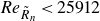 $ \textit{Re}_{\tilde {R}_n} \lt 25912$
),
$ \textit{Re}_{\tilde {R}_n} \lt 25912$
), $G_{a,\textit{first}}$
is larger than
$G_{a,\textit{first}}$
is larger than $G_{a,\textit{streaks}}$
. At
$G_{a,\textit{streaks}}$
. At $\tilde {R}_n = 0.7\,\mathrm{mm}$
,
$\tilde {R}_n = 0.7\,\mathrm{mm}$
, $G_{a,\textit{first}}$
and
$G_{a,\textit{first}}$
and $G_{a,\textit{streaks}}$
are almost the same. For
$G_{a,\textit{streaks}}$
are almost the same. For $\tilde {R}_n \gt 0.7\,\mathrm{mm}$
,
$\tilde {R}_n \gt 0.7\,\mathrm{mm}$
, $G_{a,\textit{streaks}}$
surpasses
$G_{a,\textit{streaks}}$
surpasses $G_{a,\textit{first}}$
. A similar pattern is observed in the results from the experiment by Lysenko (Reference Lysenko1990). The Reynolds number based on the transition onset location in the experiment,
$G_{a,\textit{first}}$
. A similar pattern is observed in the results from the experiment by Lysenko (Reference Lysenko1990). The Reynolds number based on the transition onset location in the experiment, $ \textit{Re}_{T}$
, is plotted as a function of
$ \textit{Re}_{T}$
, is plotted as a function of $ \textit{Re}_{\tilde {R}_n}$
in figure 16(b). In the experiment, the critical nose radius is approximately
$ \textit{Re}_{\tilde {R}_n}$
in figure 16(b). In the experiment, the critical nose radius is approximately $0.5\,\mathrm{mm}$
(
$0.5\,\mathrm{mm}$
( $ \textit{Re}_{\tilde {R}_n} \approx 18508$
), beyond which the transition onset location moves upstream. Although the values of
$ \textit{Re}_{\tilde {R}_n} \approx 18508$
), beyond which the transition onset location moves upstream. Although the values of $G_a$
do not directly reflect the real transition onset location, the good agreement indicates that, under the current experimental conditions, the dominant transition mechanism may shift from the oblique first mode to streamwise streaks as
$G_a$
do not directly reflect the real transition onset location, the good agreement indicates that, under the current experimental conditions, the dominant transition mechanism may shift from the oblique first mode to streamwise streaks as $\tilde {R}_n$
increases, which is a promising explanation for transition reversal. This also indicates that transition reversal is governed by linear mechanisms.
$\tilde {R}_n$
increases, which is a promising explanation for transition reversal. This also indicates that transition reversal is governed by linear mechanisms.
(a) Variation of $G_a$
associated with the oblique first mode and streamwise streaks as a function of
$G_a$
associated with the oblique first mode and streamwise streaks as a function of $ \textit{Re}_{\tilde {R}_n}$
. (b) Experimental results adapted from Lysenko (Reference Lysenko1990).
$ \textit{Re}_{\tilde {R}_n}$
. (b) Experimental results adapted from Lysenko (Reference Lysenko1990).

4.2.5. Effects of disturbance amplitude of acoustic waves
For the results presented in previous sections, the acoustic wave amplitude was assumed to be frequency-independent, which differs from actual wind tunnel environments. However, the validity of the results and conclusions remains unchanged when the amplitude is treated as a function of $\tilde {\omega }$
, as will be demonstrated in this subsection.
$\tilde {\omega }$
, as will be demonstrated in this subsection.
Balakumar & Chou (Reference Balakumar and Chou2018) proposed the following fitted relation to determine the disturbance amplitude at a given frequency:
 \begin{align} \tilde {A}_{\textit{amp}} / \tilde {p}_{\infty }= \begin{cases} \sqrt {C_L \tilde {\omega }^{-1} \Delta \tilde {\omega } / 2} & \text{for } 10\,\mathrm{kHz} \leqslant \tilde {\omega } \leqslant 40\,\mathrm{kHz}, \\[5pt] \sqrt {C_U \tilde {\omega }^{-3.5} \Delta \tilde {\omega } / 2} & \text{for } \tilde {\omega } \gt 40\,\mathrm{kHz}, \end{cases} \end{align}
where $C_L=3.953 \times 10^{-4}$
and
$C_L=3.953 \times 10^{-4}$
and $C_U=126.5 \times 10^6$
are constants, and
$C_U=126.5 \times 10^6$
are constants, and $\tilde {A}_{\textit{amp}}$
denotes the frequency-dependent dimensional amplitude. This empirical relation (4.1) has also been validated across different Mach number ranges (Duan et al. Reference Duan2019). In the present work, since only the relative values of
$\tilde {A}_{\textit{amp}}$
denotes the frequency-dependent dimensional amplitude. This empirical relation (4.1) has also been validated across different Mach number ranges (Duan et al. Reference Duan2019). In the present work, since only the relative values of $G_a$
are important, the values of disturbance amplitude for different frequencies can be normalised by the value of
$G_a$
are important, the values of disturbance amplitude for different frequencies can be normalised by the value of $\tilde {A}_{\textit{amp}}$
at a reference frequency of
$\tilde {A}_{\textit{amp}}$
at a reference frequency of $\tilde {\omega } = 1\,\mathrm{kHz}$
. Consequently, the choice of
$\tilde {\omega } = 1\,\mathrm{kHz}$
. Consequently, the choice of $\Delta \tilde {\omega }$
becomes irrelevant. The normalised amplitude is henceforth denoted as
$\Delta \tilde {\omega }$
becomes irrelevant. The normalised amplitude is henceforth denoted as ${A}_{\textit{amp}}$
. It should be noted that the empirical relation (4.1) provided by Balakumar & Chou (Reference Balakumar and Chou2018) does not explicitly cover the range
${A}_{\textit{amp}}$
. It should be noted that the empirical relation (4.1) provided by Balakumar & Chou (Reference Balakumar and Chou2018) does not explicitly cover the range $\tilde {\omega } \lt 10\,\mathrm{kHz}$
. However, results from Duan et al. (Reference Duan2019) suggest that
$\tilde {\omega } \lt 10\,\mathrm{kHz}$
. However, results from Duan et al. (Reference Duan2019) suggest that $\tilde {A}_{\textit{amp}}$
remains nearly constant within the range
$\tilde {A}_{\textit{amp}}$
remains nearly constant within the range $1\,\mathrm{kHz} \leqslant \tilde {\omega } \lt 10\,\mathrm{kHz}$
. Therefore, for
$1\,\mathrm{kHz} \leqslant \tilde {\omega } \lt 10\,\mathrm{kHz}$
. Therefore, for $\tilde {\omega } \lt 10\,\mathrm{kHz}$
,
$\tilde {\omega } \lt 10\,\mathrm{kHz}$
, ${A}_{\textit{amp}}$
is assumed to be equal to the value at
${A}_{\textit{amp}}$
is assumed to be equal to the value at $\tilde {\omega } = 10\,\mathrm{kHz}$
.
$\tilde {\omega } = 10\,\mathrm{kHz}$
.
The new contours of $G_a$
with adjusted disturbance amplitude are shown in figure 17. The results for the first mode and streaks are very similar to those obtained under the frequency-independent amplitude assumption. First, since the disturbance amplitudes are normalised by the value at 1 kHz, the values of
$G_a$
with adjusted disturbance amplitude are shown in figure 17. The results for the first mode and streaks are very similar to those obtained under the frequency-independent amplitude assumption. First, since the disturbance amplitudes are normalised by the value at 1 kHz, the values of $G_{a,\textit{streaks}}$
(corresponding to
$G_{a,\textit{streaks}}$
(corresponding to $\tilde {\omega } = 1\,\mathrm{kHz}$
) remain unchanged. Second, for the first mode (
$\tilde {\omega } = 1\,\mathrm{kHz}$
) remain unchanged. Second, for the first mode ( $\tilde {\omega } = 16.351\,\mathrm{kHz}$
), the value of
$\tilde {\omega } = 16.351\,\mathrm{kHz}$
), the value of $G_{a,\textit{first}}$
decreases by approximately 40 %. However, for cases with a small nose radius, such as
$G_{a,\textit{first}}$
decreases by approximately 40 %. However, for cases with a small nose radius, such as ${\mathrm{R}01}_{A}$
and
${\mathrm{R}01}_{A}$
and ${\mathrm{R}02}_{A}$
, although
${\mathrm{R}02}_{A}$
, although $G_{a,\textit{first}}$
decreases, the first mode remains the dominant instability mechanism because the streaks are too weak. For cases with a large nose radius, the streaks become more dominant as the first mode is weaker with realistic disturbance amplitudes. Therefore, the conclusion in § 4.2.4 remains unchanged.
$G_{a,\textit{first}}$
decreases, the first mode remains the dominant instability mechanism because the streaks are too weak. For cases with a large nose radius, the streaks become more dominant as the first mode is weaker with realistic disturbance amplitudes. Therefore, the conclusion in § 4.2.4 remains unchanged.
The most notable discrepancy between figures 3 and 17 is that the peaks corresponding to the entropy-layer instability disappear. This is because the associated frequencies are high ( ${\sim}$
80–200 kHz), resulting in significantly reduced
${\sim}$
80–200 kHz), resulting in significantly reduced ${A}_{\textit{amp}}$
and
${A}_{\textit{amp}}$
and $G_a$
values. The receptivity gain for the entropy-layer instability is now five orders of magnitude lower than that for the first mode or streamwise streaks. For scenarios with small amplitude free stream disturbances, instabilities undergo linear amplification before entering the nonlinear stage. Therefore, we believe that the entropy-layer instability is unlikely to significantly influence the transition reversal process under the current geometry and flow conditions. Nonetheless, the high-frequency entropy-layer instability may still play a role in the breakdown of streaks leading to turbulence and could be of greater significance in other geometries such as blunt cones. These aspects will be systematically investigated in a future study.
$G_a$
values. The receptivity gain for the entropy-layer instability is now five orders of magnitude lower than that for the first mode or streamwise streaks. For scenarios with small amplitude free stream disturbances, instabilities undergo linear amplification before entering the nonlinear stage. Therefore, we believe that the entropy-layer instability is unlikely to significantly influence the transition reversal process under the current geometry and flow conditions. Nonetheless, the high-frequency entropy-layer instability may still play a role in the breakdown of streaks leading to turbulence and could be of greater significance in other geometries such as blunt cones. These aspects will be systematically investigated in a future study.
Contours of $G_a$
in the boundary layer on the flat plate in response to free stream slow acoustic waves with zero angle of incidence for cases (a)
$G_a$
in the boundary layer on the flat plate in response to free stream slow acoustic waves with zero angle of incidence for cases (a) ${\mathrm{R}01}_{A}$
, (b)
${\mathrm{R}01}_{A}$
, (b) ${\mathrm{R}02}_{A}$
, (c)
${\mathrm{R}02}_{A}$
, (c) ${\mathrm{R}05}_{A}$
, (d)
${\mathrm{R}05}_{A}$
, (d) ${\mathrm{R}07}_{A}$
, (e)
${\mathrm{R}07}_{A}$
, (e) ${\mathrm{R}1}_{A}$
and (f)
${\mathrm{R}1}_{A}$
and (f) ${\mathrm{R}2}_{A}$
. The acoustic wave amplitude is determined via (4.1).
${\mathrm{R}2}_{A}$
. The acoustic wave amplitude is determined via (4.1).

Figure 17. Long description
Panel A: A heat map showing the distribution of values in the boundary layer on a flat plate in response to free stream slow acoustic waves with zero angle of incidence. The x-axis represents the variable k3 ranging from 0 to 10, and the y-axis represents the frequency in kHz ranging from 1 to 100. The color scale on the right indicates the log10 of the values, with blue representing lower values and red representing higher values. The heat map shows a concentration of higher values at lower frequencies and smaller k3 values, transitioning to lower values as both frequency and k3 increase. Panel B: Similar to Panel A, this heat map shows a slightly different distribution with higher values concentrated at lower frequencies and smaller k3 values, but with a more pronounced spread of higher values. Panel C: This heat map shows a more uniform distribution of values across the frequency and k3 range, with higher values more evenly spread out. Panel D: This heat map shows a concentration of higher values at lower frequencies and smaller k3 values, with a gradual transition to lower values as both frequency and k3 increase. Panel E: Similar to Panel D, this heat map shows a slightly different distribution with higher values concentrated at lower frequencies and smaller k3 values, but with a more pronounced spread of higher values. Panel F: This heat map shows a more uniform distribution of values across the frequency and k3 range, with higher values more evenly spread out.
4.3. Response to free stream vorticity waves and entropy waves at zero angle of incidence
This section presents the results for free stream entropy and vorticity disturbances at zero angle of incidence. For these waves, we also assume a frequency-independent disturbance amplitude, since no experimentally measured PSD data in the atmospheric environment are available.
Contours of $G_e$
in the boundary layer on the flat plate in response to free stream entropy waves with zero angle of incidence for cases (a)
$G_e$
in the boundary layer on the flat plate in response to free stream entropy waves with zero angle of incidence for cases (a) ${\mathrm{R}01}_{E}$
, (b)
${\mathrm{R}01}_{E}$
, (b) ${\mathrm{R}02}_{E}$
, (c)
${\mathrm{R}02}_{E}$
, (c) ${\mathrm{R}05}_{E}$
, (d)
${\mathrm{R}05}_{E}$
, (d) ${\mathrm{R}07}_{E}$
, (e)
${\mathrm{R}07}_{E}$
, (e) ${\mathrm{R}1}_{E}$
and (f)
${\mathrm{R}1}_{E}$
and (f) ${\mathrm{R}2}_{E}$
.
${\mathrm{R}2}_{E}$
.

Contours of $G_v$
in the boundary layer on the flat plate in response to free stream vorticity waves with zero angle of incidence for cases (a)
$G_v$
in the boundary layer on the flat plate in response to free stream vorticity waves with zero angle of incidence for cases (a) ${\mathrm{R}01}_{V}$
, (b)
${\mathrm{R}01}_{V}$
, (b) ${\mathrm{R}02}_{V}$
, (c)
${\mathrm{R}02}_{V}$
, (c) ${\mathrm{R}05}_{V}$
, (d)
${\mathrm{R}05}_{V}$
, (d) ${\mathrm{R}07}_{V}$
, (e)
${\mathrm{R}07}_{V}$
, (e) ${\mathrm{R}1}_{V}$
and (f)
${\mathrm{R}1}_{V}$
and (f) ${\mathrm{R}2}_{V}$
.
${\mathrm{R}2}_{V}$
.

Figures 18 and 19 present the gain contours for entropy and vorticity disturbances, respectively. For the oblique first mode, the gain values for both disturbance types are significantly lower than those associated with acoustic forcing, especially for small nose radius cases. Therefore, the boundary layer is more susceptible to slow acoustic waves than to vorticity or entropy waves, which is consistent with previous studies (Balakumar & Kegerise Reference Balakumar and Kegerise2011; Balakumar Reference Balakumar2015; He & Zhong Reference He and Zhong2022). However, in contrast to the second mode results reported by He & Zhong (Reference He and Zhong2022), the oblique first mode does not weaken as $\tilde {R}_n$
increases, which requires further investigation. Regarding streamwise streaks, the results for both disturbances are similar to those for slow acoustic waves, where
$\tilde {R}_n$
increases, which requires further investigation. Regarding streamwise streaks, the results for both disturbances are similar to those for slow acoustic waves, where $G_{{streaks}}$
increases with
$G_{{streaks}}$
increases with $\tilde {R}_n$
. For a given
$\tilde {R}_n$
. For a given $\tilde {R}_n$
,
$\tilde {R}_n$
, $G_{e,{streaks}}$
for entropy disturbances is slightly higher than that for slow acoustic disturbances. For example, in case
$G_{e,{streaks}}$
for entropy disturbances is slightly higher than that for slow acoustic disturbances. For example, in case $\mathrm{R}2$
,
$\mathrm{R}2$
, $G_{e,{streaks}}$
reaches approximately
$G_{e,{streaks}}$
reaches approximately $3.6 \times 10^6$
for entropy waves, compared with
$3.6 \times 10^6$
for entropy waves, compared with $3.1 \times 10^6$
for
$3.1 \times 10^6$
for $G_{a,\textit{streaks}}$
and
$G_{a,\textit{streaks}}$
and $1.9 \times 10^6$
for
$1.9 \times 10^6$
for $G_{v,{streaks}}$
. These findings are consistent with the DNS results of Guo (Reference Guo2025), which report that, for a blunted plate, entropy waves lead to the earliest transition, followed by acoustic waves then vorticity waves. Furthermore, the preferential streak wavenumber,
$G_{v,{streaks}}$
. These findings are consistent with the DNS results of Guo (Reference Guo2025), which report that, for a blunted plate, entropy waves lead to the earliest transition, followed by acoustic waves then vorticity waves. Furthermore, the preferential streak wavenumber, $k_3$
, is identical to that observed for acoustic disturbances, suggesting that the preferential spanwise wavenumber is independent of forcing type for medium to large nose radii.
$k_3$
, is identical to that observed for acoustic disturbances, suggesting that the preferential spanwise wavenumber is independent of forcing type for medium to large nose radii.
Most importantly, results for entropy and vorticity waves also show a shift in the dominant instability, although the changeover nose radius differs from that in cases with slow acoustic forcing. For case $\mathrm{R}01$
, the oblique first mode dominates for both disturbances. For
$\mathrm{R}01$
, the oblique first mode dominates for both disturbances. For $\tilde {R}_n \gt 0.2\,\mathrm{mm}\,(\textit{Re}_{\tilde {R}_n} \gt 7403)$
,
$\tilde {R}_n \gt 0.2\,\mathrm{mm}\,(\textit{Re}_{\tilde {R}_n} \gt 7403)$
, $G_{{streaks}}$
exceeds
$G_{{streaks}}$
exceeds $G_{\textit{first}}$
in both disturbance cases. The results suggest that the transition reversal phenomenon may also occur in a free stream environment, where vorticity and entropy waves are the dominant disturbances, although the critical value of
$G_{\textit{first}}$
in both disturbance cases. The results suggest that the transition reversal phenomenon may also occur in a free stream environment, where vorticity and entropy waves are the dominant disturbances, although the critical value of $ \textit{Re}_{\tilde {R}_n}$
may be different. However, in the study by Zhao & Dong (Reference Zhao and Dong2025), the non-modal disturbances induced by vorticity waves weaken as the nose radius increases. This discrepancy likely arises from the different formulations of the incident vortical waves. To uniquely determine the three velocity components of the vortical disturbance, Zhao & Dong (Reference Zhao and Dong2025) introduced an additional assumption by explicitly specifying the vertical vorticity (
$ \textit{Re}_{\tilde {R}_n}$
may be different. However, in the study by Zhao & Dong (Reference Zhao and Dong2025), the non-modal disturbances induced by vorticity waves weaken as the nose radius increases. This discrepancy likely arises from the different formulations of the incident vortical waves. To uniquely determine the three velocity components of the vortical disturbance, Zhao & Dong (Reference Zhao and Dong2025) introduced an additional assumption by explicitly specifying the vertical vorticity ( $\hat {\varOmega }_2 \equiv k_3 \hat {u}_{\infty } - k_1 \hat {w}_{\infty }$
). This results in a specific formulation of the incident wave that differs from the model adopted in the present study, which may be the primary cause of the observed differences in non-modal growth trends.
$\hat {\varOmega }_2 \equiv k_3 \hat {u}_{\infty } - k_1 \hat {w}_{\infty }$
). This results in a specific formulation of the incident wave that differs from the model adopted in the present study, which may be the primary cause of the observed differences in non-modal growth trends.
The generation mechanisms for streaks on the nose induced by entropy and vorticity waves are analogous to those for slow acoustic waves. Figure 20 shows the velocity perturbations on the nose for cases ${\mathrm{R}2}_A$
,
${\mathrm{R}2}_A$
, ${\mathrm{R}2}_E$
and
${\mathrm{R}2}_E$
and ${\mathrm{R}2}_V$
. Streaks are also generated via the lift-up mechanism, and the profiles and evolution of the velocity perturbations are similar in all cases, differing only in magnitude.
${\mathrm{R}2}_V$
. Streaks are also generated via the lift-up mechanism, and the profiles and evolution of the velocity perturbations are similar in all cases, differing only in magnitude.
Profiles of velocity perturbations along the wall-normal direction at different $\phi$
on the nose for cases
$\phi$
on the nose for cases ${\mathrm{R}2}_A$
,
${\mathrm{R}2}_A$
, ${\mathrm{R}2}_E$
and
${\mathrm{R}2}_E$
and ${\mathrm{R}2}_V$
. The first, second, third and fourth columns are respectively for
${\mathrm{R}2}_V$
. The first, second, third and fourth columns are respectively for $\phi = 0^\circ$
(along the stagnation line),
$\phi = 0^\circ$
(along the stagnation line), $\phi = 30^\circ$
,
$\phi = 30^\circ$
, $\phi = 60^\circ$
and
$\phi = 60^\circ$
and $\phi = 90^\circ$
(
$\phi = 90^\circ$
( $x = 0$
). All plots are for
$x = 0$
). All plots are for $k_3 = 3.6$
and
$k_3 = 3.6$
and $\tilde {\omega } = 1\,\mathrm{kHz}$
.
$\tilde {\omega } = 1\,\mathrm{kHz}$
.

Figure 20. Long description
Panel A: Three line graphs depict velocity perturbations along the wall-normal direction for different cases and variables. The x-axis represents the magnitude of velocity perturbations, and the y-axis represents the normalized wall-normal distance. The graphs compare three different cases labeled R2E, R2A, and R2V. Panel B: Three line graphs depict velocity perturbations along the wall-normal direction for different cases and variables. The x-axis represents the magnitude of velocity perturbations, and the y-axis represents the normalized wall-normal distance. The graphs compare three different cases labeled R2E, R2A, and R2V. Panel C: Three line graphs depict velocity perturbations along the wall-normal direction for different cases and variables. The x-axis represents the magnitude of velocity perturbations, and the y-axis represents the normalized wall-normal distance. The graphs compare three different cases labeled R2E, R2A, and R2V.
4.4. Resolvent analysis
This section investigates the importance of leading-edge receptivity in transition reversal via resolvent analysis; these cases are denoted by $(\boldsymbol{\cdot })_O$
. The forcing regions are specified in § 3.4. The post-shock and upstream forcing cases are considered comparatively to isolate the respective influences of the leading edge and the shock. We demonstrate that leading-edge receptivity is essential for the continuous amplification of streaks, although it is not required to trigger transition reversal.
$(\boldsymbol{\cdot })_O$
. The forcing regions are specified in § 3.4. The post-shock and upstream forcing cases are considered comparatively to isolate the respective influences of the leading edge and the shock. We demonstrate that leading-edge receptivity is essential for the continuous amplification of streaks, although it is not required to trigger transition reversal.
First, we consider optimal forcing located downstream of the shock at $x=0$
, extending from the wall to the post-shock boundary, while the output region remains unchanged. By placing the forcing downstream of the shock and nose, the effects of the leading-edge receptivity can be removed. Figure 21 presents the optimal gain contours for different cases. As in cases with slow acoustic forcing, the first mode is also weakened as the nose radius increases. For streamwise streaks, the corresponding peaks shift to
$x=0$
, extending from the wall to the post-shock boundary, while the output region remains unchanged. By placing the forcing downstream of the shock and nose, the effects of the leading-edge receptivity can be removed. Figure 21 presents the optimal gain contours for different cases. As in cases with slow acoustic forcing, the first mode is also weakened as the nose radius increases. For streamwise streaks, the corresponding peaks shift to $k_3 = 2.0$
. Crucially, while the optimal gain for streaks at
$k_3 = 2.0$
. Crucially, while the optimal gain for streaks at $\tilde {\omega } = 1\,\mathrm{kHz}$
and
$\tilde {\omega } = 1\,\mathrm{kHz}$
and $k_3 = 2.0$
initially increases with
$k_3 = 2.0$
initially increases with $\tilde {R}_n$
, it saturates for
$\tilde {R}_n$
, it saturates for $\tilde {R}_n \geqslant 1\,\mathrm{mm}$
. This indicates that streaks do not amplify continuously with increasing nose radius, particularly for medium to large radii. Moving the forcing location towards the stagnation line does not change the conclusion, which is illustrated in figure 22, where the forcing location is shifted upstream to
$\tilde {R}_n \geqslant 1\,\mathrm{mm}$
. This indicates that streaks do not amplify continuously with increasing nose radius, particularly for medium to large radii. Moving the forcing location towards the stagnation line does not change the conclusion, which is illustrated in figure 22, where the forcing location is shifted upstream to $\phi = 30^\circ$
. The optimal gains associated with streaks also saturate as
$\phi = 30^\circ$
. The optimal gains associated with streaks also saturate as $\tilde {R}_n$
increases. Therefore, for forcing located downstream of the shock, transition reversal may still occur, as the shift in the dominant instability remains identifiable. However, the mechanism is now mostly driven by weakening the first mode and not sustained by continuous streak amplification. Figure 23 shows the forcing (panels a–c) and the response of the flow field (panels d–f) at
$\tilde {R}_n$
increases. Therefore, for forcing located downstream of the shock, transition reversal may still occur, as the shift in the dominant instability remains identifiable. However, the mechanism is now mostly driven by weakening the first mode and not sustained by continuous streak amplification. Figure 23 shows the forcing (panels a–c) and the response of the flow field (panels d–f) at $x = 100$
for the cases with optimal forcing placed at
$x = 100$
for the cases with optimal forcing placed at $x = 0$
. The forcing is in the form of streamwise vortices with most of the kinetic energy in the
$x = 0$
. The forcing is in the form of streamwise vortices with most of the kinetic energy in the $|v^\prime |$
and
$|v^\prime |$
and $|w^\prime |$
components, while the response is dominated by the
$|w^\prime |$
components, while the response is dominated by the $|u^\prime |$
component. Again, this type of energy transfer is usually attributed to the lift-up mechanism.
$|u^\prime |$
component. Again, this type of energy transfer is usually attributed to the lift-up mechanism.
Contours of $G_o$
in the boundary layer for cases (a)
$G_o$
in the boundary layer for cases (a) ${\mathrm{R}01}_{O}$
, (b)
${\mathrm{R}01}_{O}$
, (b) ${\mathrm{R}02}_{O}$
, (c)
${\mathrm{R}02}_{O}$
, (c) ${\mathrm{R}05}_{O}$
, (d)
${\mathrm{R}05}_{O}$
, (d) ${\mathrm{R}07}_{O}$
, (e)
${\mathrm{R}07}_{O}$
, (e) ${\mathrm{R}1}_{O}$
and (f)
${\mathrm{R}1}_{O}$
and (f) ${\mathrm{R}2}_{O}$
. The forcing is located at
${\mathrm{R}2}_{O}$
. The forcing is located at $x=0$
, extending from the wall to the inner edge of the shock.
$x=0$
, extending from the wall to the inner edge of the shock.

Contours of $G_o$
in the boundary layer for cases (a)
$G_o$
in the boundary layer for cases (a) ${\mathrm{R}01}_{O}$
, (b)
${\mathrm{R}01}_{O}$
, (b) ${\mathrm{R}02}_{O}$
, (c)
${\mathrm{R}02}_{O}$
, (c) ${\mathrm{R}05}_{O}$
, (d)
${\mathrm{R}05}_{O}$
, (d) ${\mathrm{R}07}_{O}$
, (e)
${\mathrm{R}07}_{O}$
, (e) ${\mathrm{R}1}_{O}$
and (f)
${\mathrm{R}1}_{O}$
and (f) ${\mathrm{R}2}_{O}$
. The forcing is located at
${\mathrm{R}2}_{O}$
. The forcing is located at $\phi =30^\circ$
, extending from the wall to the inner edge of the shock.
$\phi =30^\circ$
, extending from the wall to the inner edge of the shock.

Figure 22. Long description
Panel A: A heat map showing contours of a variable in the boundary layer for case 1. The x-axis represents k3 and the y-axis represents angular frequency in kHz. The color scale ranges from 0 to 4, indicating the magnitude of the variable. Higher values are represented by lighter colors, and lower values by darker colors. The heat map shows a gradient with higher values concentrated in the lower left corner. Panel B: A heat map showing contours of a variable in the boundary layer for case 2. The x-axis represents k3 and the y-axis represents angular frequency in kHz. The color scale ranges from 0 to 4, indicating the magnitude of the variable. Higher values are represented by lighter colors, and lower values by darker colors. The heat map shows a gradient with higher values concentrated in the lower left corner. Panel C: A heat map showing contours of a variable in the boundary layer for case 3. The x-axis represents k3 and the y-axis represents angular frequency in kHz. The color scale ranges from 0 to 4, indicating the magnitude of the variable. Higher values are represented by lighter colors, and lower values by darker colors. The heat map shows a gradient with higher values concentrated in the lower left corner. Panel D: A heat map showing contours of a variable in the boundary layer for case 4. The x-axis represents k3 and the y-axis represents angular frequency in kHz. The color scale ranges from 0 to 4, indicating the magnitude of the variable. Higher values are represented by lighter colors, and lower values by darker colors. The heat map shows a gradient with higher values concentrated in the lower left corner. Panel E: A heat map showing contours of a variable in the boundary layer for case 5. The x-axis represents k3 and the y-axis represents angular frequency in kHz. The color scale ranges from 0 to 4, indicating the magnitude of the variable. Higher values are represented by lighter colors, and lower values by darker colors. The heat map shows a gradient with higher values concentrated in the lower left corner. Panel F: A heat map showing contours of a variable in the boundary layer for case 6. The x-axis represents k3 and the y-axis represents angular frequency in kHz. The color scale ranges from 0 to 4, indicating the magnitude of the variable. Higher values are represented by lighter colors, and lower values by darker colors. The heat map shows a gradient with higher values concentrated in the lower left corner.
(a–c) Optimal forcing at $x = 0$
and (d–f) the corresponding response at
$x = 0$
and (d–f) the corresponding response at $x = 100$
for
$x = 100$
for $k_3 = 2$
and
$k_3 = 2$
and $\tilde {\omega } = 1\,\mathrm{kHz}$
for (a, d)
$\tilde {\omega } = 1\,\mathrm{kHz}$
for (a, d) $|u^\prime |$
, (b, e)
$|u^\prime |$
, (b, e) $|v^\prime |$
and (c, f)
$|v^\prime |$
and (c, f) $|w^\prime |$
.
$|w^\prime |$
.

Conversely, when optimal forcing is applied upstream of the shock, the results for streaks resemble those of the physical forcing cases (i.e. slow acoustic, entropy and vorticity waves), as shown in figure 24. As $\tilde {R}_n$
increases, the optimal gain associated with the first mode decreases, while the streak gain increases continuously, unlike the post-shock forcing cases. For
$\tilde {R}_n$
increases, the optimal gain associated with the first mode decreases, while the streak gain increases continuously, unlike the post-shock forcing cases. For $\tilde {R}_n \gt 0.2\,\mathrm{mm}\,(\textit{Re}_{\tilde {R}_n} \gt 7403)$
, streaks become the dominant instability. This changeover nose radius is similar to that for vorticity and entropy disturbances. Since realistic and optimal forcings yield similar trends in changes in gain values, we suggest that the transition reversal could be insensitive to the forcing type.
$\tilde {R}_n \gt 0.2\,\mathrm{mm}\,(\textit{Re}_{\tilde {R}_n} \gt 7403)$
, streaks become the dominant instability. This changeover nose radius is similar to that for vorticity and entropy disturbances. Since realistic and optimal forcings yield similar trends in changes in gain values, we suggest that the transition reversal could be insensitive to the forcing type.
The amplitude of the free stream optimal forcing is presented in figure 25. The slow acoustic forcing is also plotted for comparison. To facilitate comparison, the amplitudes for both cases are normalised by their respective maximum pressure amplitudes. A key feature of the optimal forcing is that it concentrates upstream of the stagnation point (outside the bow shock), with negligible amplitude elsewhere. This further demonstrates the importance of leading-edge receptivity to streak strength. The composition of the optimal forcing differs significantly from that of the acoustic wave; specifically, the $|T^\prime |$
and
$|T^\prime |$
and $|w^\prime |$
components are much less prominent, whilst the
$|w^\prime |$
components are much less prominent, whilst the $|v^\prime |$
component is non-zero.
$|v^\prime |$
component is non-zero.
The evolution of the velocity perturbations is also similar to that resulting from physical forcing, as shown in figure 26. As the flow progresses, both $|v^{\prime }_{\eta }|$
and
$|v^{\prime }_{\eta }|$
and $|w^{\prime }|$
weaken, and
$|w^{\prime }|$
weaken, and $|u^{\prime }_{\xi }|$
strengthens, producing streaks downstream of the nose via the lift-up mechanism. Thus, the generation and enhancement of streaks may also be insensitive to the type of free stream forcing. Another observation from optimal forcing cases is that, for
$|u^{\prime }_{\xi }|$
strengthens, producing streaks downstream of the nose via the lift-up mechanism. Thus, the generation and enhancement of streaks may also be insensitive to the type of free stream forcing. Another observation from optimal forcing cases is that, for $\tilde {R}_n \geqslant 0.5\,\mathrm{mm}$
, the optimal gain peaks at
$\tilde {R}_n \geqslant 0.5\,\mathrm{mm}$
, the optimal gain peaks at $k_3 \approx 3.6$
. This
$k_3 \approx 3.6$
. This $k_3$
value is similar to the preferential value identified in realistic forcing cases, suggesting that for medium to large nose radii, the wavelength selection mechanism could be independent of the free stream forcing type.
$k_3$
value is similar to the preferential value identified in realistic forcing cases, suggesting that for medium to large nose radii, the wavelength selection mechanism could be independent of the free stream forcing type.
Overall, the free stream optimal forcing yields results similar to those of the realistic free stream disturbances. However, it should be noted that the optimal perturbation shown here represents a mathematical construct to maximise energy growth and does not physically resemble realistic, naturally occurring free stream disturbances. Future studies will employ resolvent analysis with physically realisable forcing, such as the framework described by Kamal, Lakebrink & Colonius (Reference Kamal, Lakebrink and Colonius2023), to further investigate the role of different disturbance types in transition reversal.
Contours of $G_o$
in the boundary layer for cases (a)
$G_o$
in the boundary layer for cases (a) ${\mathrm{R}01}_{O}$
, (b)
${\mathrm{R}01}_{O}$
, (b) ${\mathrm{R}02}_{O}$
, (c)
${\mathrm{R}02}_{O}$
, (c) ${\mathrm{R}05}_{O}$
, (d)
${\mathrm{R}05}_{O}$
, (d) ${\mathrm{R}07}_{O}$
, (e)
${\mathrm{R}07}_{O}$
, (e) ${\mathrm{R}1}_{O}$
and (f)
${\mathrm{R}1}_{O}$
and (f) ${\mathrm{R}2}_{O}$
. The forcing is located in the free stream.
${\mathrm{R}2}_{O}$
. The forcing is located in the free stream.

Distributions of the free stream optimal forcing for case ${\mathrm{R}2}_{O}$
compared with acoustic forcing from case
${\mathrm{R}2}_{O}$
compared with acoustic forcing from case ${\mathrm{R}2}_{A}$
. The forcing is located along the grid line
${\mathrm{R}2}_{A}$
. The forcing is located along the grid line $j=631$
, upstream of the shock.
$j=631$
, upstream of the shock.

Profiles of velocity perturbations along the wall-normal direction at different $\phi$
on the nose for different
$\phi$
on the nose for different $\tilde {R}_n$
with optimal freestream forcing. The first, second, third and fourth columns are respectively for
$\tilde {R}_n$
with optimal freestream forcing. The first, second, third and fourth columns are respectively for $\phi = 0^\circ$
(along the stagnation line),
$\phi = 0^\circ$
(along the stagnation line), $\phi = 30^\circ$
,
$\phi = 30^\circ$
, $\phi = 60^\circ$
and
$\phi = 60^\circ$
and $\phi = 90^\circ$
(
$\phi = 90^\circ$
( $x = 0$
). All plots are for
$x = 0$
). All plots are for $k_3 = 3.6$
and
$k_3 = 3.6$
and $\tilde {\omega } = 1\,\mathrm{kHz}$
.
$\tilde {\omega } = 1\,\mathrm{kHz}$
.

Figure 26. Long description
The image contains multiple line graphs showing velocity perturbation profiles along the wall-normal direction for different nose radii and freestream forcing conditions. Panel A: The first column of line graphs shows the profiles for the stagnation line. The x-axis represents the absolute value of the streamwise velocity perturbation, and the y-axis represents the wall-normal direction. The graphs compare different nose radii and freestream forcing conditions. Panel B: The second column of line graphs shows the profiles for a specific angle. The x-axis represents the absolute value of the normal velocity perturbation, and the y-axis represents the wall-normal direction. The graphs compare different nose radii and freestream forcing conditions. Panel C: The third column of line graphs shows the profiles for another specific angle. The x-axis represents the absolute value of the spanwise velocity perturbation, and the y-axis represents the wall-normal direction. The graphs compare different nose radii and freestream forcing conditions. Panel D: The fourth column of line graphs shows the profiles for a different specific angle. The x-axis represents the absolute value of the spanwise velocity perturbation, and the y-axis represents the wall-normal direction. The graphs compare different nose radii and freestream forcing conditions. Each panel includes multiple lines representing different conditions, with legends indicating the specific nose radius and freestream forcing. The trends and patterns in the graphs show how the velocity perturbations vary with the wall-normal direction for different conditions.
4.5. Effects of angle of incidence of slow acoustic wave
In a typical wind-tunnel environment, the disturbances are radiated from the wall, forming non-zero values of $\theta$
relative to the model. This section investigates the influence of
$\theta$
relative to the model. This section investigates the influence of $\theta$
of a slow acoustic wave on the oblique first mode and streaks. Figure 27 shows the receptivity gain contours at
$\theta$
of a slow acoustic wave on the oblique first mode and streaks. Figure 27 shows the receptivity gain contours at $\theta = 0^{\circ }$
and
$\theta = 0^{\circ }$
and $30^{\circ }$
on both the leeward and the windward sides for cases
$30^{\circ }$
on both the leeward and the windward sides for cases ${\mathrm{R}01}_{S}$
,
${\mathrm{R}01}_{S}$
, ${\mathrm{R}07}_{S}$
and
${\mathrm{R}07}_{S}$
and ${\mathrm{R}2}_{S}$
. For
${\mathrm{R}2}_{S}$
. For $G_{a,\textit{first}}$
, changing
$G_{a,\textit{first}}$
, changing $\theta$
from
$\theta$
from $0^\circ$
to
$0^\circ$
to $30^\circ$
increases its value on the leeward side, while decreasing its value on the windward side for all cases. The change in
$30^\circ$
increases its value on the leeward side, while decreasing its value on the windward side for all cases. The change in $G_{a,\textit{streaks}}$
is visually indistinguishable from the gain contours. The two-dimensional entropy-layer instability remains weak compared to the other two instabilities. The gain contours for other values of
$G_{a,\textit{streaks}}$
is visually indistinguishable from the gain contours. The two-dimensional entropy-layer instability remains weak compared to the other two instabilities. The gain contours for other values of $\theta$
are not shown here for brevity.
$\theta$
are not shown here for brevity.
Contours of $G_a$
for cases (a)
$G_a$
for cases (a) ${\mathrm{R}01}_{S}$
, (b)
${\mathrm{R}01}_{S}$
, (b) ${\mathrm{R}07}_{S}$
and (c)
${\mathrm{R}07}_{S}$
and (c) ${\mathrm{R}2}_{S}$
. The first, second and third columns of the figure respectively correspond to
${\mathrm{R}2}_{S}$
. The first, second and third columns of the figure respectively correspond to $\theta = 0^\circ$
,
$\theta = 0^\circ$
, $\theta = 30^\circ$
(leeward) and
$\theta = 30^\circ$
(leeward) and $\theta = 30^\circ$
(windward).
$\theta = 30^\circ$
(windward).

Figure 28 shows the dependence of $G_{a,\textit{first}}$
and
$G_{a,\textit{first}}$
and $G_{a,\textit{streaks}}$
on
$G_{a,\textit{streaks}}$
on $\theta$
for all cases considered. On the leeward side, for the case
$\theta$
for all cases considered. On the leeward side, for the case ${\mathrm{R}01}_{S}$
,
${\mathrm{R}01}_{S}$
, $G_{a,\textit{first}}$
increases with
$G_{a,\textit{first}}$
increases with $\theta$
and reaches a maximum at
$\theta$
and reaches a maximum at $\theta =30^\circ$
, after which it decreases. For the case
$\theta =30^\circ$
, after which it decreases. For the case ${\mathrm{R}07}_{S}$
, the trend is similar, but the maximum of
${\mathrm{R}07}_{S}$
, the trend is similar, but the maximum of $G_{a,\textit{first}}$
occurs at
$G_{a,\textit{first}}$
occurs at $\theta =50^\circ$
; at this angle, the value for
$\theta =50^\circ$
; at this angle, the value for ${\mathrm{R}07}_{S}$
exceeds that for
${\mathrm{R}07}_{S}$
exceeds that for ${\mathrm{R}01}_{S}$
. On the windward side,
${\mathrm{R}01}_{S}$
. On the windward side, $G_{a,\textit{first}}$
decreases monotonically with
$G_{a,\textit{first}}$
decreases monotonically with $\theta$
for both cases. Similarly to
$\theta$
for both cases. Similarly to $G_{a,\textit{first}}$
, the value of
$G_{a,\textit{first}}$
, the value of $G_{a,\textit{streaks}}$
is also higher on the leeward side than on the windward side, although the difference is negligible for small
$G_{a,\textit{streaks}}$
is also higher on the leeward side than on the windward side, although the difference is negligible for small $\theta$
. As
$\theta$
. As $\theta$
increases,
$\theta$
increases, $G_{a,\textit{streaks}}$
on the leeward side increases marginally, while it remains almost constant on the windward side. Consequently, the changeover
$G_{a,\textit{streaks}}$
on the leeward side increases marginally, while it remains almost constant on the windward side. Consequently, the changeover $ \textit{Re}_{\tilde {R}_n}$
on the leeward side has a non-monotonic dependence on
$ \textit{Re}_{\tilde {R}_n}$
on the leeward side has a non-monotonic dependence on $\theta$
. It initially increases with
$\theta$
. It initially increases with $\theta$
up to a critical angle (the value of which depends on
$\theta$
up to a critical angle (the value of which depends on $\tilde {R}_n$
), beyond which it begins to decrease. On the windward side, increasing
$\tilde {R}_n$
), beyond which it begins to decrease. On the windward side, increasing $\theta$
monotonically reduces the changeover
$\theta$
monotonically reduces the changeover $ \textit{Re}_{\tilde {R}_n}$
. Nevertheless, the underlying mechanism for transition reversal – a shift in dominant instability from the first mode to streamwise streaks – remains unchanged.
$ \textit{Re}_{\tilde {R}_n}$
. Nevertheless, the underlying mechanism for transition reversal – a shift in dominant instability from the first mode to streamwise streaks – remains unchanged.
(a) $G_{{a,first}}$
as a function of
$G_{{a,first}}$
as a function of $\theta$
for cases
$\theta$
for cases ${\mathrm{R}01}_{S}$
and
${\mathrm{R}01}_{S}$
and ${\mathrm{R}07}_{S}$
. (b)
${\mathrm{R}07}_{S}$
. (b) $G_{{a,streaks}}$
as a function of
$G_{{a,streaks}}$
as a function of $\theta$
for cases
$\theta$
for cases ${\mathrm{R}07}_{S}$
and
${\mathrm{R}07}_{S}$
and ${\mathrm{R}2}_{S}$
.
${\mathrm{R}2}_{S}$
.

4.5.1. Oblique first mode
Figure 29 shows contours of $u^\prime _r$
for cases
$u^\prime _r$
for cases ${\mathrm{R}01}_{S}$
(panels a, c, e) and
${\mathrm{R}01}_{S}$
(panels a, c, e) and ${\mathrm{R}07}_{S}$
(panels b, d, f) at
${\mathrm{R}07}_{S}$
(panels b, d, f) at $\theta =10^\circ$
,
$\theta =10^\circ$
, $30^\circ$
and
$30^\circ$
and $50^\circ$
. The lower part is the leeward side and the upper part is the windward side. The transmission of the acoustic wave across the shock wave is stronger on the leeward side than on the windward side and the difference increases with
$50^\circ$
. The lower part is the leeward side and the upper part is the windward side. The transmission of the acoustic wave across the shock wave is stronger on the leeward side than on the windward side and the difference increases with $\theta$
. Figure 30 shows the variation of
$\theta$
. Figure 30 shows the variation of $|u^\prime |_{max }$
along
$|u^\prime |_{max }$
along $x$
for
$x$
for ${\mathrm{R}01}_{S}$
and
${\mathrm{R}01}_{S}$
and ${\mathrm{R}07}_{S}$
at
${\mathrm{R}07}_{S}$
at $\theta =0^\circ$
,
$\theta =0^\circ$
, $10^\circ$
,
$10^\circ$
, $30^\circ$
and
$30^\circ$
and $50^\circ$
. On the leeward side, increasing
$50^\circ$
. On the leeward side, increasing $\theta$
increases the initial perturbation amplitude near the leading edge, but delays the onset of exponential growth of the first mode. These two effects lead to the non-monotonic variation of
$\theta$
increases the initial perturbation amplitude near the leading edge, but delays the onset of exponential growth of the first mode. These two effects lead to the non-monotonic variation of $G_{a,\textit{first}}$
on the leeward side shown in figure 28. On the windward side, by contrast, any non-zero incidence angle results in a lower instability amplitude throughout the computational domain compared with the
$G_{a,\textit{first}}$
on the leeward side shown in figure 28. On the windward side, by contrast, any non-zero incidence angle results in a lower instability amplitude throughout the computational domain compared with the $\theta =0^\circ$
case. The results for the oblique first mode are consistent with previous studies on a flat plate with a sharp leading edge (Egorov, Fedorov & Soudakov Reference Egorov, Fedorov and Soudakov2005), a blunt wedge (Balakumar & Kegerise Reference Balakumar and Kegerise2011; Cerminara & Sandham Reference Cerminara and Sandham2017) and a blunt cone (Wan et al. Reference Wan, Chen, Yuan, Hu and Tu2022).
$\theta =0^\circ$
case. The results for the oblique first mode are consistent with previous studies on a flat plate with a sharp leading edge (Egorov, Fedorov & Soudakov Reference Egorov, Fedorov and Soudakov2005), a blunt wedge (Balakumar & Kegerise Reference Balakumar and Kegerise2011; Cerminara & Sandham Reference Cerminara and Sandham2017) and a blunt cone (Wan et al. Reference Wan, Chen, Yuan, Hu and Tu2022).
(a, c, e) Contours of $u^{\prime }_{r}$
for
$u^{\prime }_{r}$
for ${\mathrm{R}01}_{S}$
at (a)
${\mathrm{R}01}_{S}$
at (a) $\theta = 10^\circ$
, (c)
$\theta = 10^\circ$
, (c) $\theta = 30^\circ$
and (e)
$\theta = 30^\circ$
and (e) $\theta = 50^\circ$
. (b, d, f) Contours of
$\theta = 50^\circ$
. (b, d, f) Contours of $u^{\prime }_{r}$
for
$u^{\prime }_{r}$
for ${\mathrm{R}07}_{S}$
at (b)
${\mathrm{R}07}_{S}$
at (b) $\theta = 10^\circ$
, (d)
$\theta = 10^\circ$
, (d) $\theta = 30^\circ$
and (f)
$\theta = 30^\circ$
and (f) $\theta = 50^\circ$
. The lower half of each contour corresponds to the leeward side and the upper half is the windward side. All plots are for
$\theta = 50^\circ$
. The lower half of each contour corresponds to the leeward side and the upper half is the windward side. All plots are for $\tilde {\omega } = 16.351\,\mathrm{kHz}$
and
$\tilde {\omega } = 16.351\,\mathrm{kHz}$
and $k_3 = 0.6$
. Contours are saturated at
$k_3 = 0.6$
. Contours are saturated at $\pm 5$
to assist visualisation.
$\pm 5$
to assist visualisation.

Figure 29. Long description
Panel A: A heat map showing contours of disturbances in hypersonic flow over blunted plates at a specific condition. The x-axis represents the x-coordinate ranging from 0 to 200, and the y-axis represents the y-coordinate ranging from -40 to 40. The color scale on the right indicates the magnitude of disturbances, with blue representing lower values and red representing higher values. The contours are saturated at a specific value to assist visualization. Panel B: A heat map showing contours of disturbances in hypersonic flow over blunted plates at another specific condition. The axes and color scale are the same as in Panel A. Panel C: A heat map showing contours of disturbances in hypersonic flow over blunted plates at yet another specific condition. The axes and color scale are the same as in Panel A. Panel D: A heat map showing contours of disturbances in hypersonic flow over blunted plates at a different specific condition. The axes and color scale are the same as in Panel A. Panel E: A heat map showing contours of disturbances in hypersonic flow over blunted plates at a further specific condition. The axes and color scale are the same as in Panel A. Panel F: A heat map showing contours of disturbances in hypersonic flow over blunted plates at another specific condition. The axes and color scale are the same as in Panel A.
Evolution of $|u^{\prime }|_{{max}}$
for cases (a)
$|u^{\prime }|_{{max}}$
for cases (a) ${\mathrm{R}01}_{S}$
and (b)
${\mathrm{R}01}_{S}$
and (b) ${\mathrm{R}07}_{S}$
at
${\mathrm{R}07}_{S}$
at $\theta = 0^\circ$
,
$\theta = 0^\circ$
, $\theta = 10^\circ$
,
$\theta = 10^\circ$
, $\theta = 30^\circ$
and
$\theta = 30^\circ$
and $\theta = 50^\circ$
.
$\theta = 50^\circ$
.

4.5.2. Streamwise streaks
Figure 31 plots the contours of $u^{\prime }_r$
for case
$u^{\prime }_r$
for case ${\mathrm{R}07}_{S}$
(panels a, c, e) and case
${\mathrm{R}07}_{S}$
(panels a, c, e) and case ${\mathrm{R}2}_{S}$
(panels b, d, f) at
${\mathrm{R}2}_{S}$
(panels b, d, f) at $\theta = 10^\circ$
,
$\theta = 10^\circ$
, $30^\circ$
and
$30^\circ$
and $60^\circ$
. The transmission of the acoustic wave across the shock wave on both sides is weak, and the interactions between these transmitted waves and the boundary layer are also insignificant. This weak interaction suggests that the influence of
$60^\circ$
. The transmission of the acoustic wave across the shock wave on both sides is weak, and the interactions between these transmitted waves and the boundary layer are also insignificant. This weak interaction suggests that the influence of $\theta$
on streak amplification should be small. This is confirmed in figures 32(a) and 32(b), which plot the streamwise evolution of
$\theta$
on streak amplification should be small. This is confirmed in figures 32(a) and 32(b), which plot the streamwise evolution of $|u^\prime |_{max }$
for cases
$|u^\prime |_{max }$
for cases ${\mathrm{R}07}_{S}$
and
${\mathrm{R}07}_{S}$
and ${\mathrm{R}2}_{S}$
, respectively. For both values of
${\mathrm{R}2}_{S}$
, respectively. For both values of $\tilde {R}_n$
, as
$\tilde {R}_n$
, as $\theta$
increases, the streak amplitude slightly increases on the leeward side, but decreases on the windward side. Overall, the effects of the angle of incidence of slow acoustic waves on the strength of streaks are marginal for
$\theta$
increases, the streak amplitude slightly increases on the leeward side, but decreases on the windward side. Overall, the effects of the angle of incidence of slow acoustic waves on the strength of streaks are marginal for $\theta \leqslant 60^\circ$
.
$\theta \leqslant 60^\circ$
.
(a, c, e) Contours of $u^{\prime }_{r}$
for case
$u^{\prime }_{r}$
for case ${\mathrm{R}07}_{S}$
at (a)
${\mathrm{R}07}_{S}$
at (a) $\theta = 10^\circ$
, (c)
$\theta = 10^\circ$
, (c) $\theta = 30^\circ$
and (e)
$\theta = 30^\circ$
and (e) $\theta = 60^\circ$
. (b, d, f) contours of
$\theta = 60^\circ$
. (b, d, f) contours of $u^{\prime }_{r}$
for case
$u^{\prime }_{r}$
for case ${\mathrm{R}2}_{S}$
at (b)
${\mathrm{R}2}_{S}$
at (b) $\theta = 10^\circ$
, (d)
$\theta = 10^\circ$
, (d) $\theta = 30^\circ$
and (f)
$\theta = 30^\circ$
and (f) $\theta = 60^\circ$
. The lower half of each contour corresponds to the leeward side and the upper half is the windward side. All plots are for
$\theta = 60^\circ$
. The lower half of each contour corresponds to the leeward side and the upper half is the windward side. All plots are for $\tilde {\omega } = 1\,\mathrm{kHz}$
and
$\tilde {\omega } = 1\,\mathrm{kHz}$
and $k_3 = 3.6$
. Contours are saturated at
$k_3 = 3.6$
. Contours are saturated at $\pm 5$
to assist visualisation of the transmission of the acoustic wave across the shock.
$\pm 5$
to assist visualisation of the transmission of the acoustic wave across the shock.

Figure 31. Long description
Panel A: A contour plot shows the disturbance structures for a case at a specific nose radius. The x-axis ranges from 0 to 200, and the y-axis ranges from -40 to 40. The color scale on the right indicates the magnitude of the disturbance, with blue representing lower values and red representing higher values. The plot shows a rope-like structure in the disturbance field. Panel B: Another contour plot for the same case but focusing on different disturbance contours. The axes and color scale are similar to Panel A. The plot shows a more dispersed structure compared to Panel A. Panel C: A contour plot for a different case with a larger nose radius. The axes and color scale remain the same. The plot shows a transition from rope-like to wisp-like structures. Panel D: A contour plot for the same case as Panel C but focusing on different disturbance contours. The plot shows a more dispersed structure with some elongated features. Panel E: A contour plot for another case with an even larger nose radius. The axes and color scale are consistent with previous panels. The plot shows a more pronounced wisp-like structure. Panel F: A contour plot for the same case as Panel E but focusing on different disturbance contours. The plot shows a highly dispersed structure with elongated features.
Evolution of $|u^{\prime }|_{{max}}$
along the streamwise direction for cases (a)
$|u^{\prime }|_{{max}}$
along the streamwise direction for cases (a) ${\mathrm{R}07}_{S}$
and (b)
${\mathrm{R}07}_{S}$
and (b) ${\mathrm{R}2}_{S}$
at
${\mathrm{R}2}_{S}$
at $\theta = 0^\circ$
,
$\theta = 0^\circ$
, $\theta = 10^\circ$
,
$\theta = 10^\circ$
, $\theta = 30^\circ$
and
$\theta = 30^\circ$
and $\theta = 60^\circ$
. Both plots are for
$\theta = 60^\circ$
. Both plots are for $\tilde {\omega } = 1\,\mathrm{kHz}$
and
$\tilde {\omega } = 1\,\mathrm{kHz}$
and $k_3 = 3.6$
.
$k_3 = 3.6$
.

5. Conclusion
This work employs an LNSE solver to examine the response of a Mach 4 boundary layer over blunted flat plates with various nose radii, $\tilde {R}_n$
, to free stream slow acoustic, vorticity and entropy disturbances. Six nose radii,
$\tilde {R}_n$
, to free stream slow acoustic, vorticity and entropy disturbances. Six nose radii, $\tilde {R}_n$
, ranging from 0.1 to 2 mm, are investigated. The change in gain as
$\tilde {R}_n$
, ranging from 0.1 to 2 mm, are investigated. The change in gain as $\tilde {R}_n$
increases mirrors the transition reversal observed in the experiments by Lysenko (Reference Lysenko1990).
$\tilde {R}_n$
increases mirrors the transition reversal observed in the experiments by Lysenko (Reference Lysenko1990).
For slow acoustic disturbances, depending on $\tilde {R}_n$
, the gain contours exhibit several local maxima attributed to the oblique first mode, streamwise streaks or entropy layer instability. The entropy layer instability is considered to have a negligible effect on transition compared with the other two mechanisms due to its significantly lower gain value. When
$\tilde {R}_n$
, the gain contours exhibit several local maxima attributed to the oblique first mode, streamwise streaks or entropy layer instability. The entropy layer instability is considered to have a negligible effect on transition compared with the other two mechanisms due to its significantly lower gain value. When $\tilde {R}_n \lt 0.7\,\text{mm}$
(
$\tilde {R}_n \lt 0.7\,\text{mm}$
( $ \textit{Re}_{\tilde {R}_n} \lt 25912$
), the gain due to the oblique first mode is larger than that due to the streamwise streaks and this gain decreases as
$ \textit{Re}_{\tilde {R}_n} \lt 25912$
), the gain due to the oblique first mode is larger than that due to the streamwise streaks and this gain decreases as $\tilde {R}_n$
increases due to the stabilising effects of the entropy layer. In contrast, increasing
$\tilde {R}_n$
increases due to the stabilising effects of the entropy layer. In contrast, increasing $\tilde {R}_n$
raises the gain associated with streamwise streaks, which exceeds that of the first mode for
$\tilde {R}_n$
raises the gain associated with streamwise streaks, which exceeds that of the first mode for $\tilde {R}_n\gt 0.7\,\mathrm{mm}$
. The changes in gain values suggest that the dominant mechanism for transition may shift from the oblique first mode to streamwise streaks as
$\tilde {R}_n\gt 0.7\,\mathrm{mm}$
. The changes in gain values suggest that the dominant mechanism for transition may shift from the oblique first mode to streamwise streaks as $\tilde {R}_n$
increases, leading to transition reversal. The enhancement of streaks with increasing
$\tilde {R}_n$
increases, leading to transition reversal. The enhancement of streaks with increasing $\tilde {R}_n$
results from higher initial perturbation amplitudes along the stagnation line, indicating that receptivity is crucial in determining streak strength. Also, the generation of perturbations along the stagnation line is due to inviscid mechanisms, as the inviscid and viscous results outside of the boundary layer are similar along the stagnation line. The results for vorticity and entropy disturbances are similar to those for slow acoustic disturbances. The shift in dominant instability is also observed, although the changeover nose radius reduces to 0.2 mm (
$\tilde {R}_n$
results from higher initial perturbation amplitudes along the stagnation line, indicating that receptivity is crucial in determining streak strength. Also, the generation of perturbations along the stagnation line is due to inviscid mechanisms, as the inviscid and viscous results outside of the boundary layer are similar along the stagnation line. The results for vorticity and entropy disturbances are similar to those for slow acoustic disturbances. The shift in dominant instability is also observed, although the changeover nose radius reduces to 0.2 mm ( $ \textit{Re}_{\tilde {R}_n} \approx 7403$
). Therefore, the transition reversal could also happen in the free stream environment where vorticity and entropy disturbances dominate.
$ \textit{Re}_{\tilde {R}_n} \approx 7403$
). Therefore, the transition reversal could also happen in the free stream environment where vorticity and entropy disturbances dominate.
Resolvent analysis with optimal post-shock forcing demonstrates that streaks initiated by disturbances that originate downstream of the shock do not amplify continuously with increasing nose radius. For these cases, transition reversal can still occur, driven primarily by the weakening of the first mode rather than sustained streak amplification. In contrast, optimal free stream forcing yields continuous streak amplification as the nose radius increases, similar to physical forcing cases, thereby promoting transition reversal more effectively than post-shock forcing. In addition, the optimal free stream forcing is found to be highly localised near the stagnation line, demonstrating the importance of leading-edge receptivity.
The strength of the streaks weakens as the frequency $\tilde {\omega }$
increases for a given
$\tilde {\omega }$
increases for a given $k_3$
, and the structure of high-frequency streaks resembles the elongated structures observed in experiments. For a fixed frequency, the spanwise wavenumber
$k_3$
, and the structure of high-frequency streaks resembles the elongated structures observed in experiments. For a fixed frequency, the spanwise wavenumber $k_3$
of the most amplified streaks at a given location is determined by the local boundary layer thickness
$k_3$
of the most amplified streaks at a given location is determined by the local boundary layer thickness $\delta _h$
, specifically, by the local preferential value of
$\delta _h$
, specifically, by the local preferential value of $\delta _h/(2\pi /k_3)$
. Furthermore, results from both LNSE and resolvent analysis indicate that, for medium to large nose radii, this preferential value is independent of the free stream forcing type. However, it may depend on other factors, such as wall temperature and free stream Mach number, which are subjects of future research.
$\delta _h/(2\pi /k_3)$
. Furthermore, results from both LNSE and resolvent analysis indicate that, for medium to large nose radii, this preferential value is independent of the free stream forcing type. However, it may depend on other factors, such as wall temperature and free stream Mach number, which are subjects of future research.
The effects of the angle of incidence of the slow acoustic wave are also investigated. For the first mode, the corresponding gain increases on the leeward side before reaching a critical value of $\theta$
, which depends on
$\theta$
, which depends on $\tilde {R}_n$
. Beyond this critical
$\tilde {R}_n$
. Beyond this critical $\theta$
, the gain starts to decrease. On the windward side, the gain of the first mode is always weaker than that on the leeward side and decreases monotonically with
$\theta$
, the gain starts to decrease. On the windward side, the gain of the first mode is always weaker than that on the leeward side and decreases monotonically with $\theta$
. In contrast, the strength of streamwise streaks is found to be insensitive to the angle of incidence. Thus, the changeover nose radius for the transition reversal varies non-monotonically with
$\theta$
. In contrast, the strength of streamwise streaks is found to be insensitive to the angle of incidence. Thus, the changeover nose radius for the transition reversal varies non-monotonically with $\theta$
on the leeward side, while it decreases as
$\theta$
on the leeward side, while it decreases as $\theta$
increases on the windward side.
$\theta$
increases on the windward side.
(a–b) Effect of mesh resolution on the velocity perturbation profiles along the stagnation line for case ${\mathrm{R}01}_{A}$
at
${\mathrm{R}01}_{A}$
at $\tilde {\omega } = 16.351\,\mathrm{kHz}$
and
$\tilde {\omega } = 16.351\,\mathrm{kHz}$
and $k_3=0.6$
. (c–d) Effect of mesh resolution on the velocity perturbation profiles along the stagnation line for case
$k_3=0.6$
. (c–d) Effect of mesh resolution on the velocity perturbation profiles along the stagnation line for case ${\mathrm{R}2}_{A}$
at
${\mathrm{R}2}_{A}$
at $\tilde {\omega } = 1\,\mathrm{kHz}$
and
$\tilde {\omega } = 1\,\mathrm{kHz}$
and $k_3=3.6$
.
$k_3=3.6$
.

Figure 33. Long description
Panel A: A line graph shows the effect of mesh resolution on the velocity perturbation profiles along the stagnation line for case R01 at M = 4.95 and Re = 3281x641 and 4921x991. The x-axis represents the normalized radial distance, and the y-axis represents the normalized velocity perturbation. Two lines, one in red and one in green, represent different mesh resolutions. The lines show a similar trend, starting from zero, increasing to a peak, and then gradually decreasing. Panel B: A line graph shows the effect of mesh resolution on the velocity perturbation profiles along the stagnation line for case R01 at M = 4.95 and Re = 3281x641 and 4921x991. The x-axis represents the normalized radial distance, and the y-axis represents the normalized velocity perturbation. Two lines, one in red and one in green, represent different mesh resolutions. The lines show a similar trend, starting from zero, remaining flat for a distance, and then sharply increasing before leveling off. Panel C: A line graph shows the effect of mesh resolution on the velocity perturbation profiles along the stagnation line for case R2 at M = 4.95 and Re = 3601x641 and 5401x991. The x-axis represents the normalized radial distance, and the y-axis represents the normalized velocity perturbation. Two lines, one in red and one in green, represent different mesh resolutions. The lines show a similar trend, starting from a peak, decreasing to a trough, and then gradually increasing. Panel D: A line graph shows the effect of mesh resolution on the velocity perturbation profiles along the stagnation line for case R2 at M = 4.95 and Re = 3601x641 and 5401x991. The x-axis represents the normalized radial distance, and the y-axis represents the normalized velocity perturbation. Two lines, one in red and one in green, represent different mesh resolutions. The lines show a similar trend, starting from zero, increasing to a peak, and then gradually decreasing. An inset zooms in on the region between 50 and 100 on the x-axis, showing more detailed variations.
Several limitations of the current work suggest directions for future research. First, the analysis considers a single wall temperature and does not account for entropy-layer swallowing effects. Additionally, the current flow conditions do not support second-mode instability. Future studies could extend the analysis to include these factors. Second, while the linear framework effectively reproduces the transition reversal phenomenon, it inherently excludes nonlinear effects. Whether nonlinear effects could independently drive or significantly influence the transition reversal remains an open question. Addressing this will require full nonlinear high-fidelity simulations, which could be a subject of future work. Third, as mentioned in the introduction section, many studies suggest that surface roughness affects the transition location. However, this work focuses on the effects of nose radius and free stream disturbances. The wall is assumed to be ideally smooth with no surface roughness. Therefore, further investigations are required to study its role in the transition reversal process. Finally, extending the analysis to Hiemenz flow at various Mach numbers and applying resolvent analysis with physically realisable forcing would provide deeper insights into receptivity to different free stream disturbances.
Acknowledgements
The authors thank Dr Peixu Guo for sharing his LST code.
Funding
This work is supported by the National Natural Science Foundation of China (no. 12472239) and the Hong Kong Research Grants Council (no. 15204322 and no. 15234025).
Declaration of interests
The authors report no conflict of interest.
Appendix A. Grid independence
Grid independence is verified by comparing the results of cases ${\mathrm{R}01}_{A}$
and
${\mathrm{R}01}_{A}$
and ${\mathrm{R}2}_{A}$
on the baseline grids (see table 1) with those from a refined grid. The refined mesh is composed of 4921
${\mathrm{R}2}_{A}$
on the baseline grids (see table 1) with those from a refined grid. The refined mesh is composed of 4921 $\times$
991 grid points for case
$\times$
991 grid points for case ${\mathrm{R}01}_{A}$
and 5401
${\mathrm{R}01}_{A}$
and 5401 $\times$
991 grid points for case
$\times$
991 grid points for case ${\mathrm{R}2}_{A}$
. The grid spacing in the refined mesh is reduced by 1/3 compared with the baseline grids. Figure 33 presents the streamwise velocity perturbation along the stagnation line for case
${\mathrm{R}2}_{A}$
. The grid spacing in the refined mesh is reduced by 1/3 compared with the baseline grids. Figure 33 presents the streamwise velocity perturbation along the stagnation line for case ${\mathrm{R}01}_{A}$
at
${\mathrm{R}01}_{A}$
at $\tilde {\omega } = 16.351\,\mathrm{kHz}$
and
$\tilde {\omega } = 16.351\,\mathrm{kHz}$
and $k_3=0.6$
and for case
$k_3=0.6$
and for case ${\mathrm{R}2}_{A}$
at
${\mathrm{R}2}_{A}$
at $\tilde {\omega } = 1\,\mathrm{kHz}$
and
$\tilde {\omega } = 1\,\mathrm{kHz}$
and $k_3=3.6$
for both refined and baseline grids. The mesh refinement has no visually distinguishable effect on the velocity perturbation profiles along the stagnation line for both cases. The abrupt change at
$k_3=3.6$
for both refined and baseline grids. The mesh refinement has no visually distinguishable effect on the velocity perturbation profiles along the stagnation line for both cases. The abrupt change at $\eta /\tilde {R}_n = 0.55$
is due to the shock wave, where the perturbation values are non-physical. However, the perturbation profiles downstream of the shock wave are properly resolved with no numerical oscillation. Figure 34 shows the variation of the receptivity gain for slow acoustic disturbance cases, denoted as
$\eta /\tilde {R}_n = 0.55$
is due to the shock wave, where the perturbation values are non-physical. However, the perturbation profiles downstream of the shock wave are properly resolved with no numerical oscillation. Figure 34 shows the variation of the receptivity gain for slow acoustic disturbance cases, denoted as $G_a$
, as a function of
$G_a$
, as a function of $k_3$
for different frequencies. We conclude that the baseline grid resolution is sufficient to ensure grid independence across the parameter space of interest (
$k_3$
for different frequencies. We conclude that the baseline grid resolution is sufficient to ensure grid independence across the parameter space of interest ( $\tilde {\omega }$
and
$\tilde {\omega }$
and $k_3$
) for all nose radii.
$k_3$
) for all nose radii.
Effects of mesh resolution on variation of $G_a$
as a function of
$G_a$
as a function of $k_3$
at different frequencies for (a)
$k_3$
at different frequencies for (a) ${\mathrm{R}01}_{A}$
and (b)
${\mathrm{R}01}_{A}$
and (b) ${\mathrm{R}2}_{A}$
. The crosses denote results from the refined grid.
${\mathrm{R}2}_{A}$
. The crosses denote results from the refined grid.

Appendix B. Code validation
The current numerical framework (LNSE) is validated by reproducing results from the literature. The test case selected is the flow over a parabola from Zhong (Reference Zhong1998). Figure 35 compares the magnitude of the entropy perturbation $|s^\prime |$
along the wall obtained from the LNSE solver against the data adapted from Zhong (Reference Zhong1998). The entropy perturbation is calculated as
$|s^\prime |$
along the wall obtained from the LNSE solver against the data adapted from Zhong (Reference Zhong1998). The entropy perturbation is calculated as ${s}^\prime =({T}^\prime / {\bar {T}})-((\gamma - 1)/\gamma )({p}^\prime / \bar {p})$
. The perturbation is normalised by its value at
${s}^\prime =({T}^\prime / {\bar {T}})-((\gamma - 1)/\gamma )({p}^\prime / \bar {p})$
. The perturbation is normalised by its value at $x = -0.1$
, denoted as
$x = -0.1$
, denoted as $|{s}^\prime _0|$
. The results demonstrate excellent agreement, thereby confirming the accuracy of the present framework.
$|{s}^\prime _0|$
. The results demonstrate excellent agreement, thereby confirming the accuracy of the present framework.
Comparison of normalised entropy perturbation at the wall obtained by the LNSE solver and data adapted from Zhong (Reference Zhong1998).

Appendix C. Discretisation of the linearised N–S equations
This section presents the discretisation method for the linearised equations of perturbation. We consider the homogeneous case ( $\boldsymbol{f}^{\prime } = 0$
) for simplicity. The linearised governing equation of the perturbations now reads
$\boldsymbol{f}^{\prime } = 0$
) for simplicity. The linearised governing equation of the perturbations now reads
 \begin{align} \frac {\partial\kern-1pt\boldsymbol{Q}^{\prime }}{\partial t} = \mathcal{A}\kern-1pt\boldsymbol{Q}^{\prime }. \end{align}
The system of equations is discretised using the finite volume method. The governing equations in semi-discrete form are written as
 \begin{align} \frac {\partial\kern-1pt\boldsymbol{Q}_c^{\prime }}{\partial t} + \frac {1}{\varOmega _c} \sum _{f} \boldsymbol{S}_f \boldsymbol{\cdot }\big (\boldsymbol{F}_{f}^{\prime } - \boldsymbol{F}_{vf}^{\prime }\big ) = 0, \end{align}
where the subscripts $(\boldsymbol{\cdot })_c$
and
$(\boldsymbol{\cdot })_c$
and $(\boldsymbol{\cdot })_f$
denote cell-centred and face quantities, respectively. Here,
$(\boldsymbol{\cdot })_f$
denote cell-centred and face quantities, respectively. Here, $\varOmega _c$
is the cell volume and
$\varOmega _c$
is the cell volume and $\boldsymbol{S}_f$
is the face normal vector scaled by the face area.
$\boldsymbol{S}_f$
is the face normal vector scaled by the face area.
For the inviscid flux, a modified Steger–Warming flux vector splitting is employed. The perturbation flux at a cell face is approximated as
 \begin{align} \boldsymbol{F}_{f}^{\prime } = \bar {\boldsymbol{A}}^{+}\left (\bar {\boldsymbol{Q}}_{fL}\right ) \boldsymbol{Q}_{fL}^{\prime } + \bar {\boldsymbol{A}}^{-}\left (\bar {\boldsymbol{Q}}_{fR}\right ) \boldsymbol{Q}_{fR}^{\prime }, \end{align}
where the superscripts $(\boldsymbol{\cdot })^+$
and
$(\boldsymbol{\cdot })^+$
and $(\boldsymbol{\cdot })^-$
denote the flux Jacobian matrices associated with positive and negative eigenvalues, respectively:
$(\boldsymbol{\cdot })^-$
denote the flux Jacobian matrices associated with positive and negative eigenvalues, respectively:
 \begin{align} \bar {\boldsymbol{A}}^{\pm } = \left . \frac {\partial\kern-1pt\boldsymbol{F}^{\pm }}{\partial\kern-1pt\boldsymbol{Q}} \right |_{\bar {\boldsymbol{Q}}}. \end{align}
To achieve high-order spatial accuracy, a third-order upwind scheme is applied to both the base flow and the perturbation variables. For the interface between cells $i$
and
$i$
and $i+1$
(denoted as face
$i+1$
(denoted as face $i+1/2$
), the left-biased state is reconstructed as
$i+1/2$
), the left-biased state is reconstructed as
 \begin{align} \boldsymbol{Q}_{i+1/2,L} = -\frac {1}{6}\boldsymbol{Q}_{i-1} + \frac {5}{6}\boldsymbol{Q}_{i} + \frac {2}{6}\boldsymbol{Q}_{i+1}, \end{align}
and the right-biased state is
 \begin{align} \boldsymbol{Q}_{i+1/2,R} = \frac {2}{6}\boldsymbol{Q}_{i} + \frac {5}{6}\boldsymbol{Q}_{i+1} - \frac {1}{6}\boldsymbol{Q}_{i+2}. \end{align}
This reconstruction scheme is applied consistently to the base flow $\bar {\boldsymbol{Q}}$
for calculating the Jacobians and implicitly to the perturbation
$\bar {\boldsymbol{Q}}$
for calculating the Jacobians and implicitly to the perturbation $\boldsymbol{Q}^{\prime }$
within the linearised operator assembly.
$\boldsymbol{Q}^{\prime }$
within the linearised operator assembly.
For the viscous flux in the $x_{\kern-1pt j}$
-direction, denoted as
$x_{\kern-1pt j}$
-direction, denoted as $\boldsymbol{F}_{vj}$
, the dependence is on the primitive variables
$\boldsymbol{F}_{vj}$
, the dependence is on the primitive variables $\boldsymbol{\varphi } = (\rho , u, v, w, T)^{{T}}$
and their spatial gradients. Upon linearisation, the perturbation viscous flux is expressed as
$\boldsymbol{\varphi } = (\rho , u, v, w, T)^{{T}}$
and their spatial gradients. Upon linearisation, the perturbation viscous flux is expressed as
 \begin{align} \boldsymbol{F}_{vj}^{\prime } = \bar {\boldsymbol{M}}_{jk} \frac {\partial\kern-1pt\boldsymbol{\varphi }^{\prime }}{\partial x_k} + \bar {\boldsymbol{K}}_{j} \boldsymbol{\varphi }^{\prime }, \end{align}
where the primitive perturbation is related to the conservative perturbation via $\boldsymbol{\varphi }^{\prime } = \boldsymbol{J}^{-1}\kern-1pt\boldsymbol{Q}^{\prime }$
(Rolandi et al. Reference Rolandi, Ribeiro, Yeh and Taira2024). The matrix
$\boldsymbol{\varphi }^{\prime } = \boldsymbol{J}^{-1}\kern-1pt\boldsymbol{Q}^{\prime }$
(Rolandi et al. Reference Rolandi, Ribeiro, Yeh and Taira2024). The matrix $\bar {\boldsymbol{M}}_{jk}$
contains the base flow transport coefficients. The matrix
$\bar {\boldsymbol{M}}_{jk}$
contains the base flow transport coefficients. The matrix $\bar {\boldsymbol{K}}_{j}$
arises from the linearisation of these transport coefficients and the nonlinear viscous stress terms (e.g. dissipation function). Detailed expressions for these matrices follow the formulation of Dwivedi (Reference Dwivedi2020). The gradients
$\bar {\boldsymbol{K}}_{j}$
arises from the linearisation of these transport coefficients and the nonlinear viscous stress terms (e.g. dissipation function). Detailed expressions for these matrices follow the formulation of Dwivedi (Reference Dwivedi2020). The gradients $\partial\kern-1pt\boldsymbol{\varphi }^{\prime } / \partial x_k$
are approximated at cell faces using second-order central differences.
$\partial\kern-1pt\boldsymbol{\varphi }^{\prime } / \partial x_k$
are approximated at cell faces using second-order central differences.
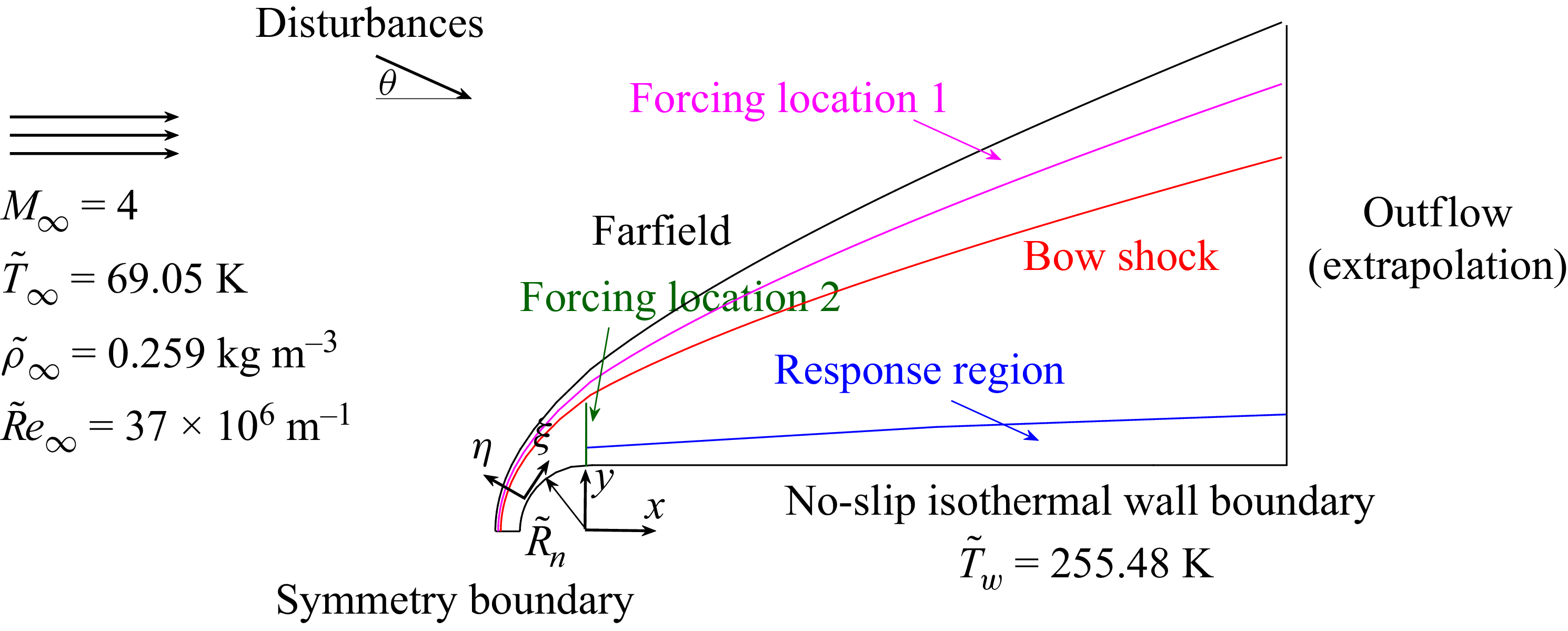
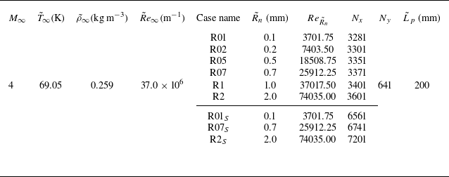
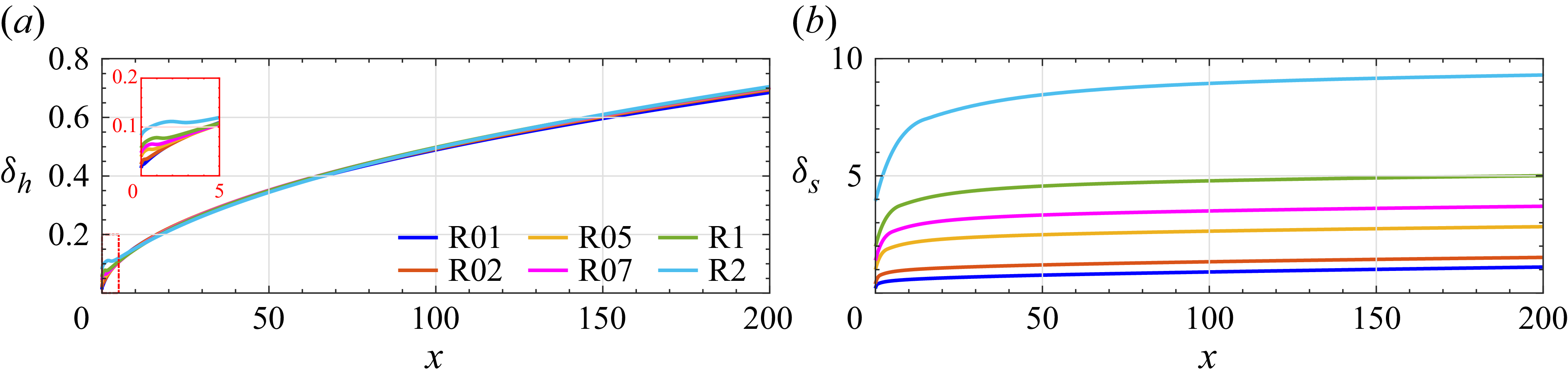
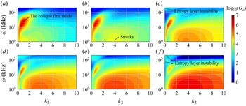
 Ga
Ga R01A
R01A R02A
R02A R05A
R05A R07A
R07A R1A
R1A R2A
R2A
 ur′
ur′ R01A
R01A −αi
−αi R01A
R01A ω~=16.351
 k3=0.6
 R01A
R01A x=100
x=100 R07A
R07A x=150
x=150 R2A
R2A x=200
x=200 ω~=16.351kHz
 k3=0.6
 ω~=16.351kHz
 k3=0.6
 R01A
R01A x=100
x=100 R07A
R07A x=150
x=150 R2A
R2A x=200
x=200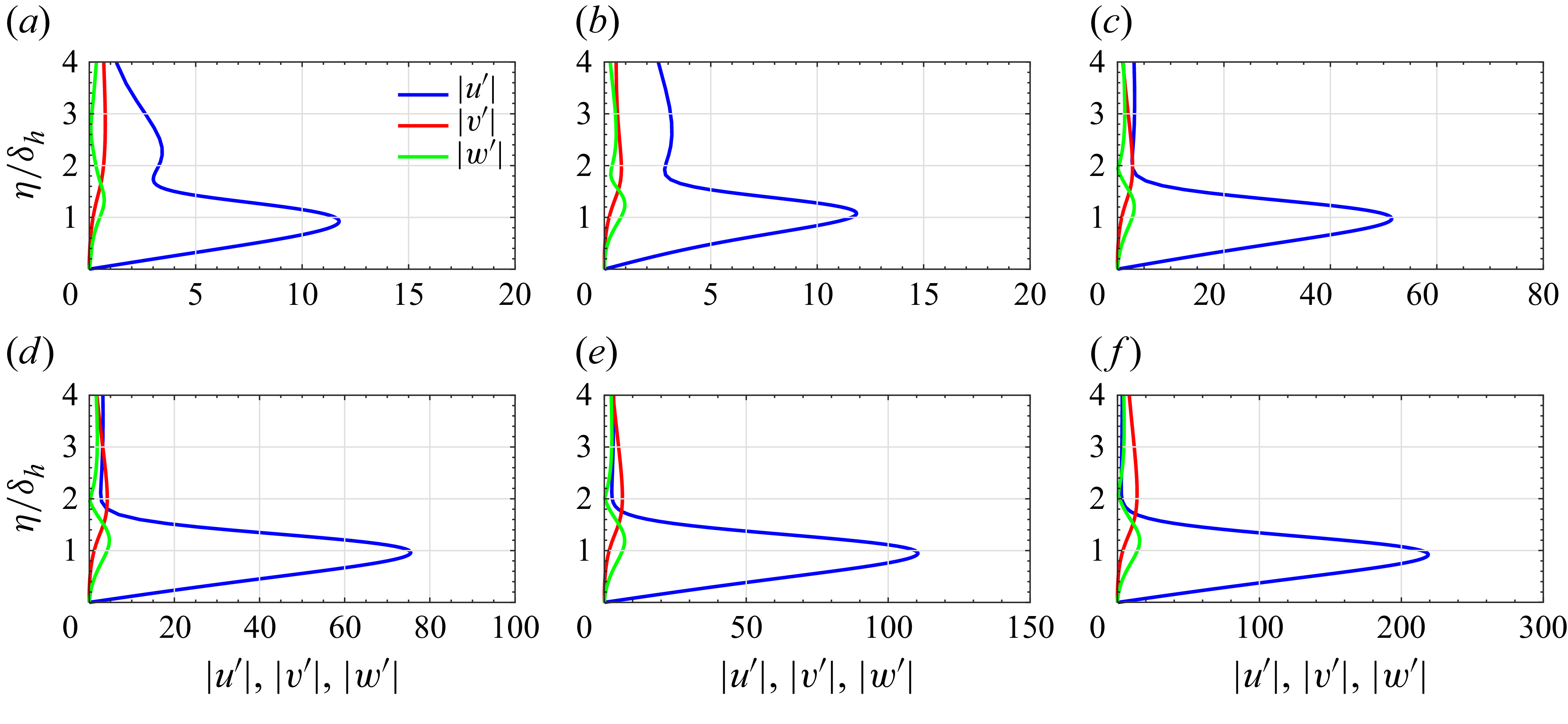
 |u′|
|u′| |v′|
|v′| |w′|
|w′| ω~=1
ω~=1 k3=3.6
 x=20
x=20 R01A
R01A R02A
R02A R05A
R05A R07A
R07A R1A
R1A R2A
R2A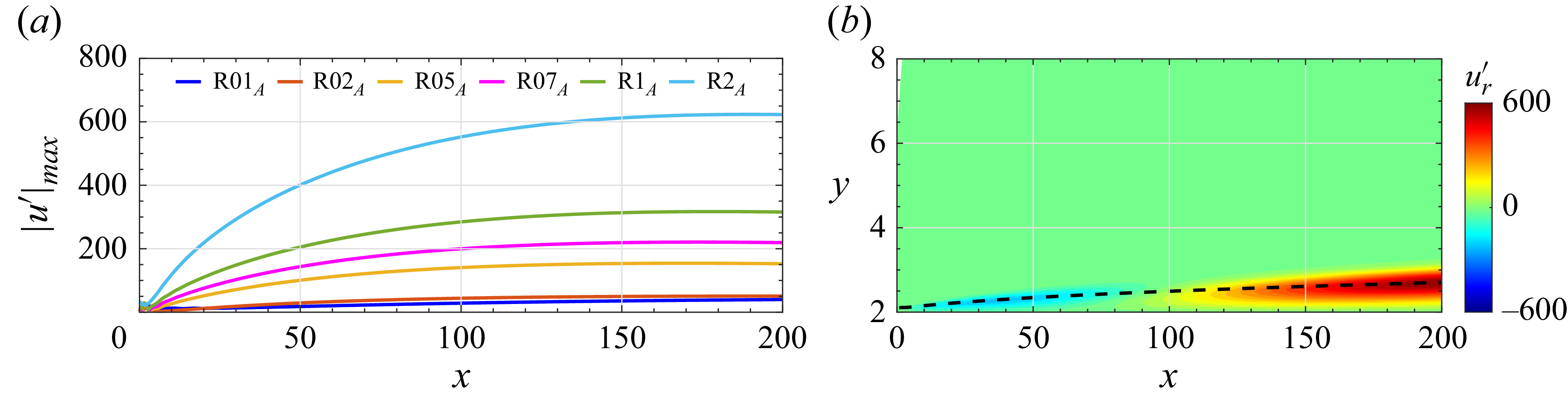
 |u′|max
 ur′
ur′ R2A
R2A ω~=1
ω~=1 k3=3.6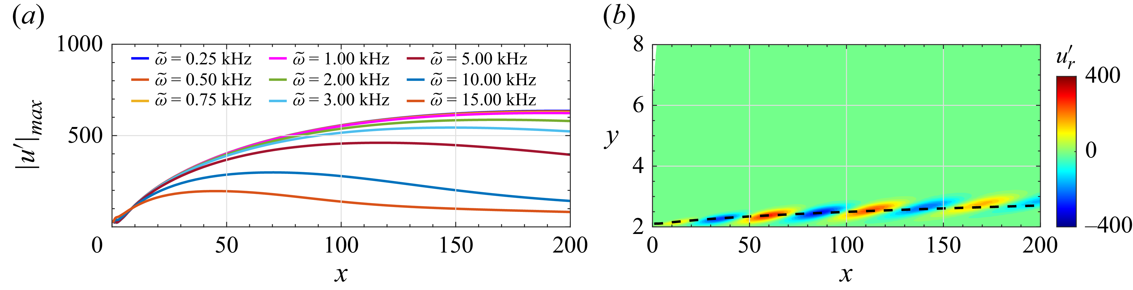
 |u′|max
 ω~
ω~ ur′
ur′ ω~=10kHz
 R2A
R2A k3=3.6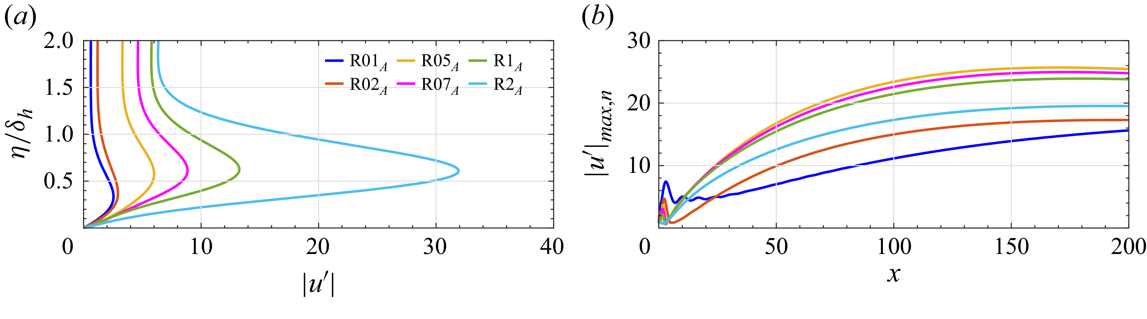
 |u′|
|u′| x
x |u′|max
 x=0
x=0 ω~=1
ω~=1 k3=3.6
 ϕ
ϕ R~n
R~n ϕ=0∘
ϕ=0∘ ϕ=30∘
ϕ=30∘ ϕ=60∘
ϕ=60∘ ϕ=90∘
ϕ=90∘ x=0
x=0 k3=3.6
 ω~=1kHz
 R2A
R2A R2A,inv
 k3=3.6
 ω~=1kHz
 ϖξ,r′
ϖξ,r′ vη,r′
vη,r′ wr′
wr′
 |u′|max
 k3
k3 R2A
R2A |u′|max
 δh/(2π/k3)
 x=0
x=0 ω~=1kHz
 Tr′
Tr′ R05A
R05A R2A
R2A ±
± ω~=200
 k3=0
k3=0
 ur′
ur′ R05A
R05A R2A
R2A ±
± ω~=200
 k3=0
k3=0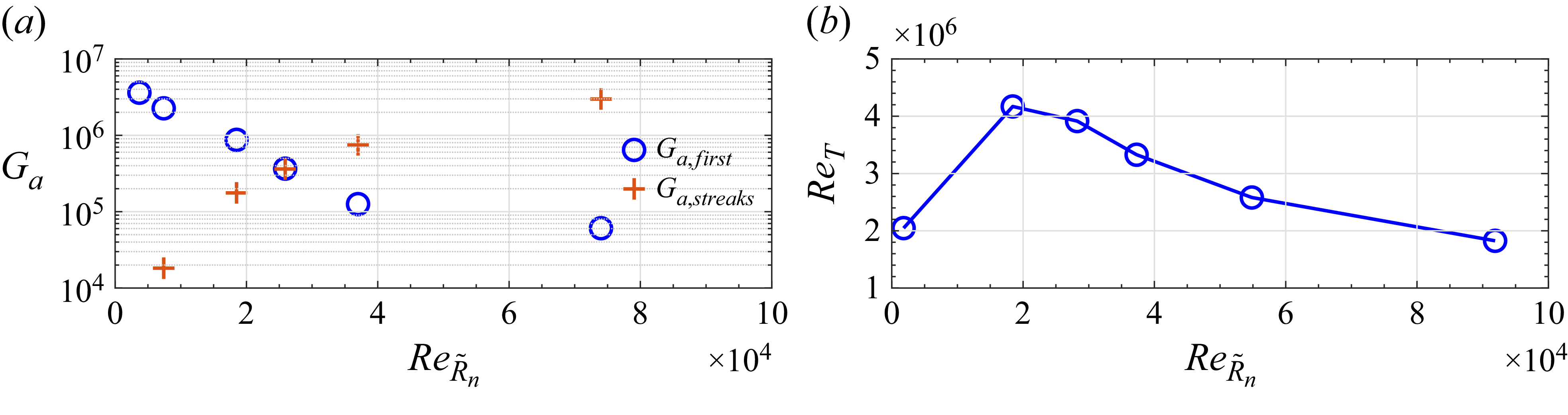
 Ga
Ga ReR~n
ReR~n
 Ga
Ga R01A
R01A R02A
R02A R05A
R05A R07A
R07A R1A
R1A R2A
R2A
 Ge
Ge R01E
R01E R02E
R02E R05E
R05E R07E
R07E R1E
R1E R2E
R2E
 Gv
Gv R01V
R01V R02V
R02V R05V
R05V R07V
R07V R1V
R1V R2V
R2V
 ϕ
ϕ R2A
R2A R2E
R2E R2V
R2V ϕ=0∘
ϕ=0∘ ϕ=30∘
ϕ=30∘ ϕ=60∘
ϕ=60∘ ϕ=90∘
ϕ=90∘ x=0
x=0 k3=3.6
 ω~=1kHz
 Go
Go R01O
R01O R02O
R02O R05O
R05O R07O
R07O R1O
R1O R2O
R2O x=0
x=0
 Go
Go R01O
R01O R02O
R02O R05O
R05O R07O
R07O R1O
R1O R2O
R2O ϕ=30∘
ϕ=30∘
 x=0
x=0 x=100
x=100 k3=2
k3=2 ω~=1kHz
 |u′|
|u′| |v′|
|v′| |w′|
|w′|
 Go
Go R01O
R01O R02O
R02O R05O
R05O R07O
R07O R1O
R1O R2O
R2O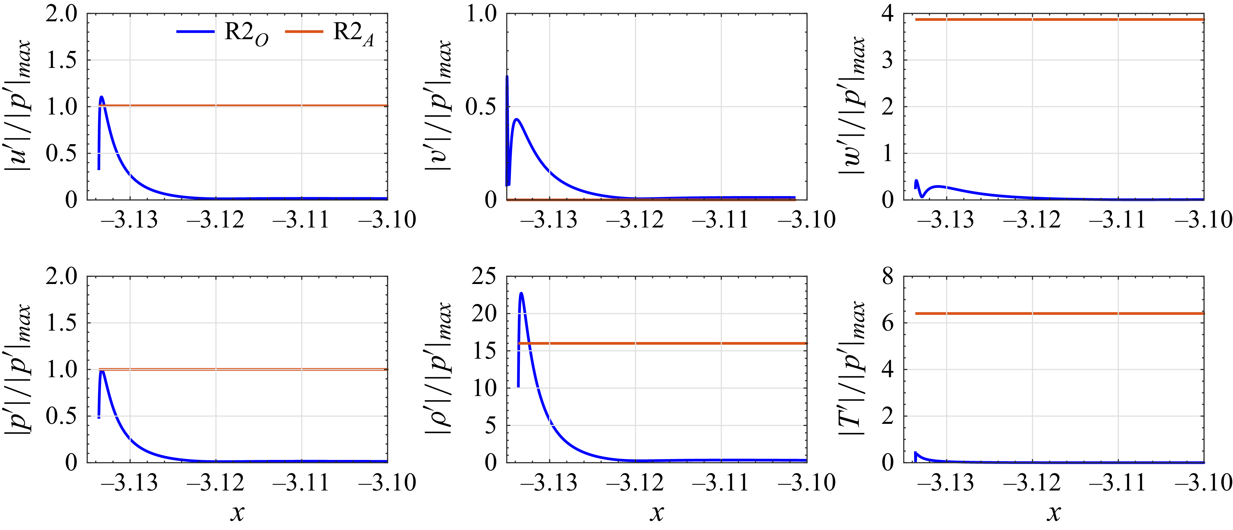
 R2O
R2O R2A
R2A j=631
j=631
 ϕ
ϕ R~n
R~n ϕ=0∘
ϕ=0∘ ϕ=30∘
ϕ=30∘ ϕ=60∘
ϕ=60∘ ϕ=90∘
ϕ=90∘ x=0
x=0 k3=3.6
 ω~=1kHz
 Ga
Ga R01S
R01S R07S
R07S R2S
R2S θ=0∘
θ=0∘ θ=30∘
θ=30∘ θ=30∘
θ=30∘
 Ga,first
 θ
θ R01S
R01S R07S
R07S Ga,streaks
 θ
θ R07S
R07S R2S
R2S
 ur′
ur′ R01S
R01S θ=10∘
θ=10∘ θ=30∘
θ=30∘ θ=50∘
θ=50∘ ur′
ur′ R07S
R07S θ=10∘
θ=10∘ θ=30∘
θ=30∘ θ=50∘
θ=50∘ ω~=16.351kHz
 k3=0.6
 ±5
±5
 |u′|max
 R01S
R01S R07S
R07S θ=0∘
θ=0∘ θ=10∘
θ=10∘ θ=30∘
θ=30∘ θ=50∘
θ=50∘
 ur′
ur′ R07S
R07S θ=10∘
θ=10∘ θ=30∘
θ=30∘ θ=60∘
θ=60∘ ur′
ur′ R2S
R2S θ=10∘
θ=10∘ θ=30∘
θ=30∘ θ=60∘
θ=60∘ ω~=1kHz
 k3=3.6
 ±5
±5
 |u′|max
 R07S
R07S R2S
R2S θ=0∘
θ=0∘ θ=10∘
θ=10∘ θ=30∘
θ=30∘ θ=60∘
θ=60∘ ω~=1kHz
 k3=3.6
 R01A
R01A ω~=16.351kHz
 k3=0.6
 R2A
R2A ω~=1kHz
 k3=3.6
 Ga
Ga k3
k3 R01A
R01A R2A
R2A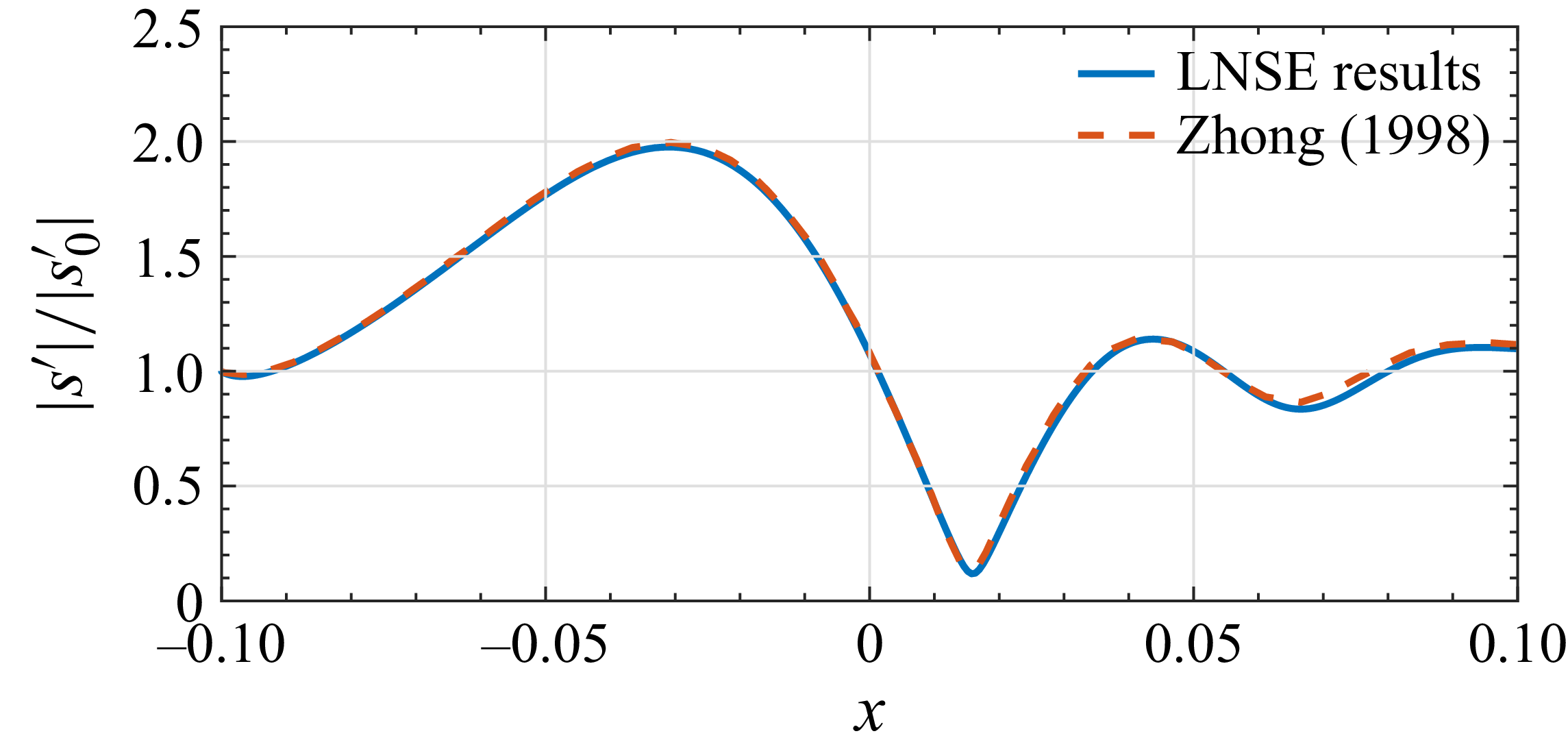

 Open access

