


1 Introduction
The flow of an annular film on the outside of a rotating circular cylinder is a fascinating and much-studied problem. It finds numerous applications in industry from its uses in spin coating in microfabrication to rotational moulding (Ruschak Reference Ruschak1985). Rotational flows have received extensive attention since the early work of Yih (Reference Yih1960), who studied the problem of a rotating drum partially submerged in a liquid bath, both experimentally and theoretically using a linear stability analysis. In the same year Phillips (Reference Phillips1960) analysed the linear stability of a related system, where the drum was partially filled, under the assumption that the system was inviscid, and compared against experimental results. Pedley (Reference Pedley1967) similarly analysed inviscid, rotating, free-surface flow on the inside or outside of a cylinder in the linear regime.
The nonlinear problem was originally modelled by Moffatt (Reference Moffatt1977), inspired by the question of what volume of honey can sustainably be held on a rotating knife. By assuming the film to be thin, and incorporating the effects of gravity and rotation only, Moffatt solved this by finding limiting solutions for given parameters. Pukhnachev (Reference Pukhnachev1977) developed a similar thin-film model that incorporated the effects of surface tension. While both considered the case of flow on the outside of a cylinder (coating flow), the leading-order equations derived are equally valid for flow on the inside of a cylinder (rimming flow). Indeed the latter problem has also proven of be of significant interest (Thoroddsen & Mahadevan Reference Thoroddsen and Mahadevan1997; Hosoi & Mahadevan Reference Hosoi and Mahadevan1999). However, at higher orders, the models are not equivalent (Lopes, Thiele & Hazel Reference Lopes, Thiele and Hazel2018); our focus here will be on coating flows.
A full treatment of the problem requires a model that incorporates the subtle interplay of gravity, surface tension, viscous effects, inertia (including centrifugation), rotational effects and potentially even dewetting effects (Thiele Reference Thiele2011; Lin et al. Reference Lin, Rogers, Tseluiko and Thiele2016) (all other models, including the ones derived herein, implicitly assume complete wetting). As a result, since the pioneering work of Moffatt and Pukhnachev, many authors have extended this coating flow problem. For example, in their original form the thin-film equations did not even conserve the mass of fluid in the system; this was resolved by Evans, Schwartz & Roy (Reference Evans, Schwartz and Roy2004) by extending the thin-film solution to an additional order. Benilov & O’Brien (Reference Benilov and O’Brien2005), Noakes, King & Riley (Reference Noakes, King and Riley2006) and Kelmanson (Reference Kelmanson2009) incorporated inertia into the model, while Weidner, Schwartz & Eres (Reference Weidner, Schwartz and Eres1997) and Evans, Schwartz & Roy (Reference Evans, Schwartz and Roy2005) extended the model to three dimensions in the absence and presence of cylinder rotation, respectively. Reisfeld & Bankoff (Reference Reisfeld and Bankoff1992) incorporated non-isothermal effects, showing that, for a heated cylinder, thermocapillarity would act in concert with gravity, speeding the draining effect, or the reverse for cooled cylinders.
The solutions to these models have been investigated at length. Pukhnachov (Reference Pukhnachov2005a,Reference Pukhnachovb) and Karabut (Reference Karabut2007) studied the existence and uniqueness of steady state solutions to the thin-film equations. Kelmanson (Reference Kelmanson2009) examined how the incorporation of inertia affected these results, showing that it caused the location of the maximum point to be displaced downwards. Recently, Lopes et al. (Reference Lopes, Thiele and Hazel2018) investigated the steady state solutions to the Moffatt problem by means of both a finite-element-based Stokes solver, and a reduced-order model derived using a variational approach. In both cases the parameter space was explored using numerical path continuation. They were able to identify regimes for weak surface tension that supported up to four solutions for a single set of parameters. Notably classical models displayed no multiplicity of solutions, while the variational model displayed at most two solutions for a given set of parameters. The authors attributed this to the improved hydrostatic approximation, as the variational model retains the complete curvature in the capillary term.
For sufficiently thin films at high rotation rates the film is close to solid-body rotation; the deviation of the period of the film from the period of the rotation of the cylinder is a subtle phenomenon that has been investigated both analytically (Hinch & Kelmanson Reference Hinch and Kelmanson2003; Kelmanson Reference Kelmanson2009) and using sophisticated numerical algorithms (Groh & Kelmanson Reference Groh and Kelmanson2009, Reference Groh and Kelmanson2012, Reference Groh and Kelmanson2014). It has also been observed that the models support shock-like solutions: such structures, and the approach to them, have been a particular focus in recent years (Wilson, Hunt & Duffy Reference Wilson, Hunt and Duffy2002; Hinch, Kelmanson & Metcalfe Reference Hinch, Kelmanson and Metcalfe2004; Tougher, Wilson & Duffy Reference Tougher, Wilson and Duffy2009).
As pointed out by Wray, Papageorgiou & Matar (Reference Wray, Papageorgiou and Matar2017b), a common assumption used by most lubrication models is that the thickness of a film is small relative to both the characteristic wavelength of disturbances to the flow, and to the radii of curvature of the substrate. Indeed, this is the case for all models discussed thus far. However, this is quite a stringent assumption, imposing, in particular, a parabolic flow profile that is inappropriately restrictive for all but the thinnest films. Indeed the preliminary results of Peterson, Jimack & Kelmanson (Reference Peterson, Jimack and Kelmanson2001) showed, as expected, increasing error for the lubrication model of Pukhnachev (Reference Pukhnachev1977) for increasing film thicknesses. As a consequence the majority of studies looking at thick layers have relied on numerical computation of the velocity profiles (Hansen & Kelmanson Reference Hansen and Kelmanson1994). In the absence of inertia, Wray et al. (Reference Wray, Papageorgiou and Matar2017b) were able to derive a low-order model that gave good agreement with direct numerical simulations (DNS) by relaxing the assumption on the radius of curvature and using the weighted residual integral boundary-layer (WRIBL) formulation of Ruyer-Quil & Manneville (Reference Ruyer-Quil and Manneville2000). The method of weighted residuals is essentially a separation-of-variables, Galerkin-type approach in which a coupled pair of evolution equations is determined for the local film height  $h$ and depth-integrated liquid flux $q$. While successful in its original intended purpose of improving the modelling of inertia in falling film flows on a plane (Ruyer-Quil & Manneville Reference Ruyer-Quil and Manneville2000; Scheid, Ruyer-Quil & Manneville Reference Scheid, Ruyer-Quil and Manneville2006; Chakraborty et al. Reference Chakraborty, Nguyen, Ruyer-Quil and Bontozoglou2014), the technique has also proven to result in excellent agreement with both DNS and experimental results in flows on a fibre (Ruyer-Quil et al. Reference Ruyer-Quil, Treveleyan, Giorgiutti-Dauphiné, Duprat and Kalliadasis2008), as well as in flows incorporating other physical effects such as thermocapillarity (Kalliadasis et al. Reference Kalliadasis, Demekhin, Ruyer-Quil and Velarde2003), electrostatic effects (Wray, Matar & Papageorgiou Reference Wray, Matar and Papageorgiou2017a) or blowing and suction (Thompson, Tseluiko & Papageorgiou Reference Thompson, Tseluiko and Papageorgiou2016). Notably, the full second-order model is rather complicated (Ruyer-Quil & Manneville Reference Ruyer-Quil and Manneville2000), requiring the solution of four coupled equations. Via a complex Padé regularisation procedure, Scheid et al. (Reference Scheid, Ruyer-Quil and Manneville2006) were able to deduce a simpler ‘regularised’ two-equation model that was fully consistent at second order. However, in this (Scheid et al. Reference Scheid, Ruyer-Quil and Manneville2006) and other (Wray et al. Reference Wray, Matar and Papageorgiou2017a) contexts it was seen that this regularised model offered little or no improvement in accuracy over the ‘simplified model’ derived by neglecting second-order inertial effects; it is therefore this simplified model on which the thick-film model of Wray et al. (Reference Wray, Papageorgiou and Matar2017b) is based.
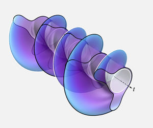
Experiments (Moffatt Reference Moffatt1977; Preziosi & Joseph Reference Preziosi and Joseph1988; Melo & Douady Reference Melo and Douady1993; Kelmanson Reference Kelmanson1995; de Bruyn Reference de Bruyn1997), thin-film models (Kelmanson Reference Kelmanson1995; Evans et al. Reference Evans, Schwartz and Roy2005) and linear stability analyses (Noakes, King & Riley Reference Noakes, King and Riley2005; Benilov & Lapin Reference Benilov and Lapin2013) have shown that the fluid layer coating the rotating cylinder can be unstable to axial perturbations for sufficiently high rotation rates. In particular, in his experiments involving syrup, Moffatt (Reference Moffatt1977) observed that this resulted in the formation of asymmetric ‘syrup rings’ spaced regularly in the axial direction. The model described here may be readily extended to the three-dimensional situation, but for the moment we confine our attention to two-dimensional flows. This is an important preliminary step in both validation and gaining understanding before investigating the three-dimensional case. Furthermore, in the presence of external effects (such as electric fields) the natural instabilities may be purely two-dimensional.
The intent of the paper is twofold: first, to develop and validate a model suitable for thick fluid flows, and second, to investigate the parametric behaviour of the system. In this context ‘thick’ indicates that the radius of curvature of the substrate is of the same order as the thickness of the film. In the past attention has primarily been focussed on the regimes accessible to thin-film models; we extend this here. Therefore we begin by formulating the problem in § 2. We derive the low-order model in § 3. In § 4 we validate our model against an Orr–Sommerfeld analysis in the linear regime, and against DNS in the nonlinear regime. Both the low-order model and the DNS are then used to explore parameter space (the computational methods for which are explained in detail in §§ A.1, A.3 and A.3). We examine some of the details of modelling flows on curved substrates in § 4.4. Finally we give our conclusions in § 5.
2 Problem formulation
2.1 Governing equations
Consider the flow of an incompressible liquid of density  $\unicode[STIX]{x1D70C}$ and dynamic viscosity $\unicode[STIX]{x1D707}$ hanging from a cylinder of radius $R$ rotating with angular velocity $C_{V}$. We assume that the gas–liquid interface has constant surface tension coefficient $\unicode[STIX]{x1D70E}$. The axis of the cylinder is aligned horizontally, with the gravity $\boldsymbol{g}$ acting vertically. We work in cylindrical coordinates centred on the axis of the cylinder and neglect all variations and velocities in the axial direction. We non-dimensionalise the system as
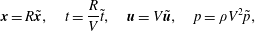 $$\begin{eqnarray}\boldsymbol{x}=R\tilde{\boldsymbol{x}},\quad t=\frac{R}{V}\tilde{t},\quad \boldsymbol{u}=V\tilde{\boldsymbol{u}},\quad p=\unicode[STIX]{x1D70C}V^{2}\tilde{p},\end{eqnarray}$$
 where  $\boldsymbol{u}=(u,v)$ is the usual velocity in polar coordinates and $p$ is the pressure. We use the gravity-based scaling for velocity
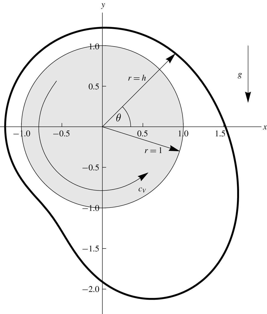
  $V=\sqrt{Rg}$ so as to explicitly retain a dimensionless rotation rate as a system parameter. The system is shown schematically in figure 1.
Geometry of the problem considered in the present work. The disk has unit radius, with the interface lying at  $r=h$. Gravity acts vertically downwards. The disk rotates with angular velocity $c_{V}$ in the anti-clockwise direction.
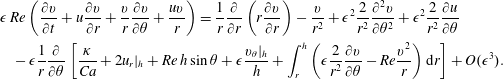
Discarding the tilde notation, the system is governed by the Navier–Stokes and continuity equations,
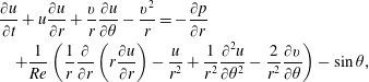 $$\begin{eqnarray}\displaystyle & & \displaystyle \frac{\unicode[STIX]{x2202}u}{\unicode[STIX]{x2202}t}+u\frac{\unicode[STIX]{x2202}u}{\unicode[STIX]{x2202}r}+\frac{v}{r}\frac{\unicode[STIX]{x2202}u}{\unicode[STIX]{x2202}\unicode[STIX]{x1D703}}-\frac{v^{2}}{r}=-\frac{\unicode[STIX]{x2202}p}{\unicode[STIX]{x2202}r}\nonumber\\ \displaystyle & & \displaystyle \quad +\frac{1}{Re}\left(\frac{1}{r}\frac{\unicode[STIX]{x2202}}{\unicode[STIX]{x2202}r}\left(r\frac{\unicode[STIX]{x2202}u}{\unicode[STIX]{x2202}r}\right)-\frac{u}{r^{2}}+\frac{1}{r^{2}}\frac{\unicode[STIX]{x2202}^{2}u}{\unicode[STIX]{x2202}\unicode[STIX]{x1D703}^{2}}-\frac{2}{r^{2}}\frac{\unicode[STIX]{x2202}v}{\unicode[STIX]{x2202}\unicode[STIX]{x1D703}}\right)-\sin \unicode[STIX]{x1D703},\end{eqnarray}$$
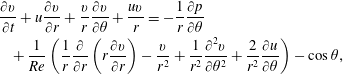 $$\begin{eqnarray}\displaystyle & & \displaystyle \frac{\unicode[STIX]{x2202}v}{\unicode[STIX]{x2202}t}+u\frac{\unicode[STIX]{x2202}v}{\unicode[STIX]{x2202}r}+\frac{v}{r}\frac{\unicode[STIX]{x2202}v}{\unicode[STIX]{x2202}\unicode[STIX]{x1D703}}+\frac{uv}{r}=-\frac{1}{r}\frac{\unicode[STIX]{x2202}p}{\unicode[STIX]{x2202}\unicode[STIX]{x1D703}}\nonumber\\ \displaystyle & & \displaystyle \quad +\,\frac{1}{Re}\left(\frac{1}{r}\frac{\unicode[STIX]{x2202}}{\unicode[STIX]{x2202}r}\left(r\frac{\unicode[STIX]{x2202}v}{\unicode[STIX]{x2202}r}\right)-\frac{v}{r^{2}}+\frac{1}{r^{2}}\frac{\unicode[STIX]{x2202}^{2}v}{\unicode[STIX]{x2202}\unicode[STIX]{x1D703}^{2}}+\frac{2}{r^{2}}\frac{\unicode[STIX]{x2202}u}{\unicode[STIX]{x2202}\unicode[STIX]{x1D703}}\right)-\cos \unicode[STIX]{x1D703},\end{eqnarray}$$
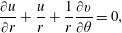 $$\begin{eqnarray}\frac{\unicode[STIX]{x2202}u}{\unicode[STIX]{x2202}r}+\frac{u}{r}+\frac{1}{r}\frac{\unicode[STIX]{x2202}v}{\unicode[STIX]{x2202}\unicode[STIX]{x1D703}}=0,\end{eqnarray}$$
 while at the interface  $r=h$ the tangential stress condition is
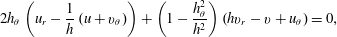 $$\begin{eqnarray}2h_{\unicode[STIX]{x1D703}}\left(u_{r}-\frac{1}{h}\left(u+v_{\unicode[STIX]{x1D703}}\right)\right)+\left(1-\frac{h_{\unicode[STIX]{x1D703}}^{2}}{h^{2}}\right)\left(hv_{r}-v+u_{\unicode[STIX]{x1D703}}\right)=0,\end{eqnarray}$$
the normal stress condition is
 $$\begin{eqnarray}\left(\frac{1}{We}\unicode[STIX]{x1D705}-p\right)(h^{2}+h_{\unicode[STIX]{x1D703}}^{2})=\frac{1}{Re}\left(-2h^{2}u_{r}-2h_{\unicode[STIX]{x1D703}}(v-u_{\unicode[STIX]{x1D703}}-hv_{r})-2\frac{h_{\unicode[STIX]{x1D703}}^{2}}{h}(v_{\unicode[STIX]{x1D703}}+u)\right),\end{eqnarray}$$
and the kinematic condition, together with the continuity equation and impermeability at the cylinder wall, imply
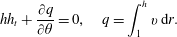 $$\begin{eqnarray}hh_{t}+\frac{\unicode[STIX]{x2202}q}{\unicode[STIX]{x2202}\unicode[STIX]{x1D703}}=0,\quad q=\int _{1}^{h}v\,\text{d}r.\end{eqnarray}$$
The no-slip and impermeability conditions are
 $$\begin{eqnarray}v|_{r=1}=c_{V},\quad u|_{r=1}=0.\end{eqnarray}$$
Our system is thus governed by the dimensionless groups
 $$\begin{eqnarray}Re=\frac{\unicode[STIX]{x1D70C}VR}{\unicode[STIX]{x1D707}},\quad We=\frac{\unicode[STIX]{x1D70C}V^{2}R}{\unicode[STIX]{x1D70E}},\quad c_{R}=h|_{t=0},\quad c_{V}=\frac{R}{V}C_{V},\end{eqnarray}$$
respectively a Reynolds number representing the relative significance of inertia compared to viscous effects, a Weber number encoding the balance of inertial effects to surface tension, the undisturbed (uniform) radius of the interface, and the angular velocity of the disk (in this study always positive and thus rotating in an anticlockwise sense). We note that on occasion it will be useful to consider the Capillary number
 $$\begin{eqnarray}Ca=\frac{We}{Re}=\frac{\unicode[STIX]{x1D707}V}{\unicode[STIX]{x1D70E}},\end{eqnarray}$$
which gives the relative significance of viscous effects compared to surface tension, as this is often used in some of the cited literature.
3 Modelling
We begin by deriving a thick-film long-wave model. As detailed by Wray et al. (Reference Wray, Papageorgiou and Matar2017b), first a boundary-layer-like equation is derived. While we are of course not studying a boundary layer, the terminology is common due to structural similarities of the equations (Ruyer-Quil & Manneville Reference Ruyer-Quil and Manneville2000; Kalliadasis et al. Reference Kalliadasis, Demekhin, Ruyer-Quil and Velarde2003; Scheid et al. Reference Scheid, Ruyer-Quil and Manneville2006; Oron & Heining Reference Oron and Heining2008; Ruyer-Quil et al. Reference Ruyer-Quil, Treveleyan, Giorgiutti-Dauphiné, Duprat and Kalliadasis2008; Wray et al. Reference Wray, Matar and Papageorgiou2017a). Key to this process is that the thickness of the film is allowed to be of the same order as the radius of curvature of the substrate, hence being a ‘thick-film’ model. Then a low-order model is derived by applying the method of weighted residuals (Ruyer-Quil & Manneville Reference Ruyer-Quil and Manneville2000). Our dimensional scaling is slightly different here to that used by Wray et al. (Reference Wray, Papageorgiou and Matar2017b), however, as we allow  $Re=O(1)$ it does not affect the long-wave scalings.
3.1 Long-wave boundary-layer equation
In order to make analytic progress, we use the long-wave methodology proposed by Wray et al. (Reference Wray, Papageorgiou and Matar2017b). In particular, the substitutions
 $$\begin{eqnarray}\displaystyle u\mapsto \unicode[STIX]{x1D716}u,\quad \unicode[STIX]{x2202}_{\unicode[STIX]{x1D703}}\mapsto \unicode[STIX]{x1D716}\unicode[STIX]{x2202}_{\unicode[STIX]{x1D703}},\quad \unicode[STIX]{x2202}_{t}\mapsto \unicode[STIX]{x1D716}\unicode[STIX]{x2202}_{t}, & & \displaystyle\end{eqnarray}$$
 are made, where  $\unicode[STIX]{x1D716}$ is a small parameter. Following the standard terminology of Ruyer-Quil & Manneville (Reference Ruyer-Quil and Manneville2000), this is an ‘ordering parameter’ which serves only to assert the relative size of a particular term. In particular, it does not constitute an actual physical rescaling of space; it is merely an assertion about the relative sizes of terms and their derivatives. The technique is discussed further by Kalliadasis et al. (Reference Kalliadasis, Ruyer-Quil, Scheid and Velarde2011, Chap. 6) (see also Thompson et al. (Reference Thompson, Tseluiko and Papageorgiou2016), Trevelyan, Pereira & Kalliadasis (Reference Trevelyan, Pereira and Kalliadasis2012)). This approach has been used and validated extensively, giving excellent results (Ruyer-Quil & Manneville Reference Ruyer-Quil and Manneville2000; Kalliadasis et al. Reference Kalliadasis, Demekhin, Ruyer-Quil and Velarde2003; Scheid et al. Reference Scheid, Ruyer-Quil and Manneville2006; Oron & Heining Reference Oron and Heining2008; Ruyer-Quil et al. Reference Ruyer-Quil, Treveleyan, Giorgiutti-Dauphiné, Duprat and Kalliadasis2008; Wray et al. Reference Wray, Matar and Papageorgiou2017a). We note that the streamwise (azimuthal) coordinate has a fixed domain length of $2\unicode[STIX]{x03C0}$ which may cast doubt on the validity of the long-wave assumption; indeed, there are certain possible flows that could violate the stated asymptotic approximations. However, there are many physical contexts in which azimuthal variations would be of higher order. These include situations where a field variable depends only on the radial coordinate to leading order, situations where the radius of the cylinder is large relative to thickness of the film, and situations where a film varies slowly on the $[\!0,2\unicode[STIX]{x03C0}\!)$ domain (save perhaps in some small matching/shock region, where the asymptotic assumptions are violated, and yet the results are of appreciable accuracy nonetheless (Mazouchi & Homsy Reference Mazouchi and Homsy2001; Gaskell et al. Reference Gaskell, Jimack, Sellier, Thompson and Wilson2004)). In contexts where the assumptions are in fact violated, the derived system may be treated as a model in the sense of Kliakhandler, Davis & Bankoff (Reference Kliakhandler, Davis and Bankoff2001), where justification is provided a posteriori via extensive validation against direct numerical computations.
Under the above substitutions (3.1), the  $r$-component of the momentum equation (2.2) becomes
 $$\begin{eqnarray}\frac{\unicode[STIX]{x2202}p}{\unicode[STIX]{x2202}r}=\frac{v^{2}}{r}-\sin \unicode[STIX]{x1D703}-\frac{\unicode[STIX]{x1D716}}{Re}\left[\frac{\unicode[STIX]{x2202}}{\unicode[STIX]{x2202}r}\left(\frac{1}{r}\frac{\unicode[STIX]{x2202}v}{\unicode[STIX]{x2202}\unicode[STIX]{x1D703}}\right)+\frac{2}{r^{2}}\frac{\unicode[STIX]{x2202}v}{\unicode[STIX]{x2202}\unicode[STIX]{x1D703}}\right]+O(\unicode[STIX]{x1D716}^{2}).\end{eqnarray}$$
 Integrating this from  $r$ to $h$ subject to the first-order truncation of the normal stress,
 $$\begin{eqnarray}\frac{\unicode[STIX]{x1D705}}{We}-p=-\frac{\unicode[STIX]{x1D716}}{Re}2u_{r}+O(\unicode[STIX]{x1D716}^{2}),\end{eqnarray}$$
 and substituting into the  $\unicode[STIX]{x1D703}$-component of the momentum equation (2.3) gives the boundary-layer equation
 $$\begin{eqnarray}\displaystyle & & \displaystyle \unicode[STIX]{x1D716}\,Re\left(\frac{\unicode[STIX]{x2202}v}{\unicode[STIX]{x2202}t}+u\frac{\unicode[STIX]{x2202}v}{\unicode[STIX]{x2202}r}+\frac{v}{r}\frac{\unicode[STIX]{x2202}v}{\unicode[STIX]{x2202}\unicode[STIX]{x1D703}}+\frac{uv}{r}\right)=\frac{1}{r}\frac{\unicode[STIX]{x2202}}{\unicode[STIX]{x2202}r}\left(r\frac{\unicode[STIX]{x2202}v}{\unicode[STIX]{x2202}r}\right)-\frac{v}{r^{2}}+\unicode[STIX]{x1D716}^{2}\frac{2}{r^{2}}\frac{\unicode[STIX]{x2202}^{2}v}{\unicode[STIX]{x2202}\unicode[STIX]{x1D703}^{2}}+\unicode[STIX]{x1D716}^{2}\frac{2}{r^{2}}\frac{\unicode[STIX]{x2202}u}{\unicode[STIX]{x2202}\unicode[STIX]{x1D703}}\nonumber\\ \displaystyle & & \displaystyle \quad -\,\unicode[STIX]{x1D716}\frac{1}{r}\frac{\unicode[STIX]{x2202}}{\unicode[STIX]{x2202}\unicode[STIX]{x1D703}}\left[\frac{\unicode[STIX]{x1D705}}{Ca}+2u_{r}|_{h}+Re\,h\sin \unicode[STIX]{x1D703}+\unicode[STIX]{x1D716}\frac{v_{\unicode[STIX]{x1D703}}|_{h}}{h}+\int _{r}^{h}\left(\unicode[STIX]{x1D716}\frac{2}{r^{2}}\frac{\unicode[STIX]{x2202}v}{\unicode[STIX]{x2202}\unicode[STIX]{x1D703}}-Re\frac{v^{2}}{r}\right)\text{d}r\right]+O(\unicode[STIX]{x1D716}^{3}).\nonumber\\ \displaystyle & & \displaystyle\end{eqnarray}$$
The tangential stress condition at the interface (2.5) truncated at second order is
 $$\begin{eqnarray}v-hv_{r}=\unicode[STIX]{x1D716}^{2}\left[u_{\unicode[STIX]{x1D703}}+4h_{\unicode[STIX]{x1D703}}u_{r}\right]+O(\unicode[STIX]{x1D716}^{3}).\end{eqnarray}$$
3.2 Weighted residual model
We now develop a low-order model based on the boundary-layer equation (3.4) following the method of weighted residuals (Ruyer-Quil & Manneville Reference Ruyer-Quil and Manneville2000). The leading-order solution is determined in the same way as the classical gradient expansion, while higher orders are computed by projecting onto an appropriately expanded set of basis functions for the cross-stream coordinate  $r$. In general, the determination of these basis functions and the subsequent projection is a laborious process, but Ruyer-Quil & Manneville demonstrated that the methodology could be simplified considerably by a weighted integral procedure, with the weight $w$ being the solution to the adjoint of the leading-order problem. This accounts for the higher-order corrections to the model while avoiding the explicit determination of the higher-order basis functions or their coefficients. We therefore begin by solving the leading-order problem,
 $$\begin{eqnarray}\frac{\unicode[STIX]{x2202}}{\unicode[STIX]{x2202}r}\left(\frac{1}{r}\frac{\unicode[STIX]{x2202}}{\unicode[STIX]{x2202}r}\left(rv\right)\right)=0\quad \text{subject to}\quad v|_{r=1}=c_{V},\quad (hv_{r}-v)|_{r=h}=0.\end{eqnarray}$$
The solution to this is just solid-body rotation,
 $$\begin{eqnarray}v=c_{V}r.\end{eqnarray}$$
 To proceed to higher order, we project onto a suitable set of basis functions  $f_{n}(r)$, with the dependence on $\unicode[STIX]{x1D703}$ and $t$ given by the coefficients $a_{n}$
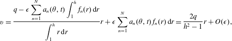 $$\begin{eqnarray}v=\frac{q-\unicode[STIX]{x1D716}\displaystyle \mathop{\sum }_{n=1}^{N}a_{n}(\unicode[STIX]{x1D703},t)\int _{1}^{h}f_{n}(r)\,\text{d}r}{\displaystyle \int _{1}^{h}r\,\text{d}r}r+\unicode[STIX]{x1D716}\mathop{\sum }_{n=1}^{N}a_{n}(\unicode[STIX]{x1D703},t)\,f_{n}(r)\,\text{d}r=\frac{2q}{h^{2}-1}r+O(\unicode[STIX]{x1D716}^{}),\end{eqnarray}$$
 where this form has been selected so as to retain the relation  $q=\int _{1}^{h}v\,\text{d}r$ correct to second order. Explicit computation of the $a_{n}$ (and their corresponding basis functions) can be avoided by a suitable choice of weighting function $w$. This weight is the solution of the adjoint of the leading-order problem, and hence depends on the problem being solved, including its geometry (Ruyer-Quil et al. Reference Ruyer-Quil, Treveleyan, Giorgiutti-Dauphiné, Duprat and Kalliadasis2008). For viscous flow on a rotating disk, this weight is (Wray et al. Reference Wray, Papageorgiou and Matar2017b)
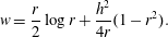 $$\begin{eqnarray}w=\frac{r}{2}\log r+\frac{h^{2}}{4r}(1-r^{2}).\end{eqnarray}$$
 Multiplying (3.4) by  $w$ and integrating across the film thickness, and observing that
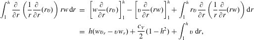 $$\begin{eqnarray}\displaystyle \int _{1}^{h}\frac{\unicode[STIX]{x2202}}{\unicode[STIX]{x2202}r}\left(\frac{1}{r}\frac{\unicode[STIX]{x2202}}{\unicode[STIX]{x2202}r}(rv)\right)rw\,\text{d}r & = & \displaystyle \left[w\frac{\unicode[STIX]{x2202}}{\unicode[STIX]{x2202}r}(rv)\right]_{1}^{h}-\left[v\frac{\unicode[STIX]{x2202}}{\unicode[STIX]{x2202}r}(rw)\right]_{1}^{h}+\int _{1}^{h}rv\frac{\unicode[STIX]{x2202}}{\unicode[STIX]{x2202}r}\left(\frac{1}{r}\frac{\unicode[STIX]{x2202}}{\unicode[STIX]{x2202}r}(rw)\right)\text{d}r\nonumber\\ \displaystyle & = & \displaystyle h(wv_{r}-vw_{r})+\frac{c_{V}}{2}(1-h^{2})+\int _{1}^{h}v\,\text{d}r,\end{eqnarray}$$
gives the final governing equation,
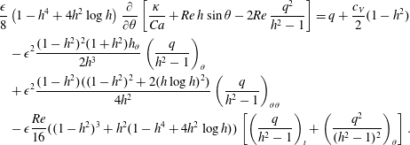 $$\begin{eqnarray}\displaystyle & & \displaystyle \hspace{-24.0pt}\frac{\unicode[STIX]{x1D716}}{8}\left(1-h^{4}+4h^{2}\log h\right)\frac{\unicode[STIX]{x2202}}{\unicode[STIX]{x2202}\unicode[STIX]{x1D703}}\left[\frac{\unicode[STIX]{x1D705}}{Ca}+Re\,h\sin \unicode[STIX]{x1D703}-2Re\,\frac{q^{2}}{h^{2}-1}\right]=q+\frac{c_{V}}{2}(1-h^{2})\nonumber\\ \displaystyle & & \displaystyle \hspace{-24.0pt}\quad -\,\unicode[STIX]{x1D716}^{2}\frac{(1-h^{2})^{2}(1+h^{2})h_{\unicode[STIX]{x1D703}}}{2h^{3}}\left(\frac{q}{h^{2}-1}\right)_{\unicode[STIX]{x1D703}}\nonumber\\ \displaystyle & & \displaystyle \hspace{-24.0pt}\quad +\,\unicode[STIX]{x1D716}^{2}\frac{(1-h^{2})((1-h^{2})^{2}+2(h\log h)^{2})}{4h^{2}}\left(\frac{q}{h^{2}-1}\right)_{\unicode[STIX]{x1D703}\unicode[STIX]{x1D703}}\nonumber\\ \displaystyle & & \displaystyle \hspace{-24.0pt}\quad -\,\unicode[STIX]{x1D716}\frac{Re}{16}((1-h^{2})^{3}+h^{2}(1-h^{4}+4h^{2}\log h))\left[\left(\frac{q}{h^{2}-1}\right)_{t}+\left(\frac{q^{2}}{(h^{2}-1)^{2}}\right)_{\unicode[STIX]{x1D703}}\right].\end{eqnarray}$$
 This represents the main novel result of the paper and, together with the kinematic condition (2.7), constitutes a closed system governing the evolution of the film thickness  $h$ and the flux $q$.
$q$.
For the purposes of the computations, we reverse the long-wave scalings (3.1) – in particular, the terms preceded by  $\unicode[STIX]{x1D716}$ are still expected to exhibit values of the appropriate order, but this rescaling avoids setting an arbitrary value for $\unicode[STIX]{x1D716}$. Note that, other than the term $-2Re(q^{2}/h^{2}-1)$ and the terms on the final line, equation (3.11) is identical to the expression given in Wray et al. (Reference Wray, Papageorgiou and Matar2017b) (up to trivial differences in scalings), incorporating the effects of capillarity, gravity, viscosity and the driving effect of the rotating cylinder. The remaining terms constitute the incorporation of inertia into the problem. We note that of particular interest is the term $-2Re(q^{2}/h^{2}-1)$: this enters via the aberrant $O(1)$ term $v^{2}/r$ in the cross-stream pressure term (3.2). Such inertial terms in the cross-stream momentum equation are typically of too small an order to enter via the pressure in other geometries (Ruyer-Quil & Manneville Reference Ruyer-Quil and Manneville2000; Oron & Heining Reference Oron and Heining2008; Ruyer-Quil et al. Reference Ruyer-Quil, Treveleyan, Giorgiutti-Dauphiné, Duprat and Kalliadasis2008); we shall see later that this term represents a centrifugal instability and its incorporation is crucial for accurate modelling.
Finally, we note that this model has two main differences to previous models in the literature: firstly, a long-wave thick-film scaling (3.1) is used to derive the boundary-layer equation (3.4); secondly the method of weighted residuals is used to derive the coupled  $h$ and
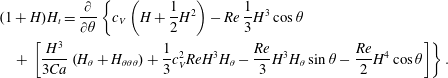
  $q$ evolution equations (2.7), (3.11). To help quantify the contribution of each of the two elements to the final model, we derive two simplified equations that each use only of these techniques. We will find that the classic thin-film gradient expansion model of Kelmanson (Reference Kelmanson2009) is recoverable as an appropriate limit of each of these equations. The relationship between the models is given schematically in figure 2.
3.2.1 Thin-film weighted residual model
An appropriate thin-film (but still weighted residual) formulation can be derived from (3.11) by applying the scalings
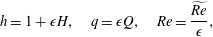 $$\begin{eqnarray}h=1+\unicode[STIX]{x1D716}H,\quad q=\unicode[STIX]{x1D716}Q,\quad Re=\frac{\widetilde{Re}}{\unicode[STIX]{x1D716}},\end{eqnarray}$$
 discarding the tilde decoration and expanding for small  $\unicode[STIX]{x1D716}$, giving
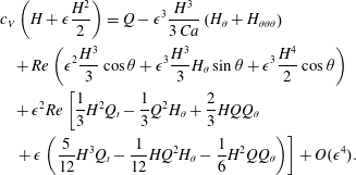 $$\begin{eqnarray}\displaystyle & & \displaystyle c_{V}\left(H+\unicode[STIX]{x1D716}\frac{H^{2}}{2}\right)=Q-\unicode[STIX]{x1D716}^{3}\frac{H^{3}}{3\,Ca}\left(H_{\unicode[STIX]{x1D703}}+H_{\unicode[STIX]{x1D703}\unicode[STIX]{x1D703}\unicode[STIX]{x1D703}}\right)\nonumber\\ \displaystyle & & \displaystyle \quad +\,Re\left(\unicode[STIX]{x1D716}^{2}\frac{H^{3}}{3}\cos \unicode[STIX]{x1D703}+\unicode[STIX]{x1D716}^{3}\frac{H^{3}}{3}H_{\unicode[STIX]{x1D703}}\sin \unicode[STIX]{x1D703}+\unicode[STIX]{x1D716}^{3}\frac{H^{4}}{2}\cos \unicode[STIX]{x1D703}\right)\nonumber\\ \displaystyle & & \displaystyle \quad +\,\unicode[STIX]{x1D716}^{2}Re\left[\frac{1}{3}H^{2}Q_{t}-\frac{1}{3}Q^{2}H_{\unicode[STIX]{x1D703}}+\frac{2}{3}HQQ_{\unicode[STIX]{x1D703}}\right.\nonumber\\ \displaystyle & & \displaystyle \left.\quad +\,\unicode[STIX]{x1D716}\left(\frac{5}{12}H^{3}Q_{t}-\frac{1}{12}HQ^{2}H_{\unicode[STIX]{x1D703}}-\frac{1}{6}H^{2}QQ_{\unicode[STIX]{x1D703}}\right)\right]+O(\unicode[STIX]{x1D716}^{4}).\end{eqnarray}$$
This is complemented by the thin-film version of the kinematic condition (2.7),
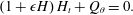 $$\begin{eqnarray}\left(1+\unicode[STIX]{x1D716}H\right)H_{t}+Q_{\unicode[STIX]{x1D703}}=0.\end{eqnarray}$$
We refer to this as the thin-film weighted residual or WRIBL model.
The relationship between the full long-wave model (equations (2.7), (3.11), § 3.2), the thin-film weighted residual model (equations (3.13), (3.14), § 3.2.1), the long-wave gradient expansion model (equation (3.18), § 3.2.2) and the thin-film gradient expansion model as derived by Kelmanson (Reference Kelmanson2009) (equation (3.19), § 3.2.3).
3.2.2 Thick-film gradient expansion model
In order to perform a gradient expansion (Ruyer-Quil & Manneville Reference Ruyer-Quil and Manneville2000), we make the substitution
 $$\begin{eqnarray}q=q_{0}+\unicode[STIX]{x1D716}q_{1}+\cdots \,.\end{eqnarray}$$
 We then solve for successive  $q_{i}$ in (3.11), giving
 $$\begin{eqnarray}\displaystyle & \displaystyle q_{0}=\frac{c_{V}}{2}\left(h^{2}-1\right), & \displaystyle\end{eqnarray}$$
 $$\begin{eqnarray}\displaystyle & \displaystyle q_{1}=\frac{1}{8}\left(1-h^{4}+4h^{2}\log h\right)\frac{\unicode[STIX]{x2202}}{\unicode[STIX]{x2202}\unicode[STIX]{x1D703}}\left(\frac{\unicode[STIX]{x1D705}}{Ca}+Re\,h\sin \unicode[STIX]{x1D703}-Re\,c_{V}^{2}\frac{h^{2}}{2}\right). & \displaystyle\end{eqnarray}$$
Substitution of these into (2.7) gives the appropriate gradient expansion model as
 $$\begin{eqnarray}\frac{1}{2}\left(h^{2}\right)_{t}=\frac{\unicode[STIX]{x2202}}{\unicode[STIX]{x2202}\unicode[STIX]{x1D703}}\left\{\frac{c_{V}}{2}(1-h^{2})+\frac{\unicode[STIX]{x1D716}}{8}\left(1-h^{4}+4h^{2}\log h\right)\frac{\unicode[STIX]{x2202}}{\unicode[STIX]{x2202}\unicode[STIX]{x1D703}}\left(Re\,c_{V}^{2}\frac{h^{2}}{2}-\frac{\unicode[STIX]{x1D705}}{Ca}-Re\,h\sin \unicode[STIX]{x1D703}\right)\right\}.\end{eqnarray}$$
 Note that the only additional terms accrued at  $O(\unicode[STIX]{x1D716}^{2})$ would arise from the inertial terms which are themselves only valid at first order and so we stop at $q_{1}$.
3.2.3 Recovery of existing models
We can recover the model (2.14) of Kelmanson (Reference Kelmanson2009) up to third order as a special case of both (3.18) and (3.13), (3.14) (and hence of the full model (2.7), (3.11)). As a consequence we can therefore recover other systems which are a specialisation of Kelmanson, such as those of Moffatt (Reference Moffatt1977) and Pukhnachev (Reference Pukhnachev1977). In particular, performing a thin-film expansion  $(h=1+\unicode[STIX]{x1D6FF}H)$ on (3.18) or a gradient expansion $(Q=Q_{0}+\unicode[STIX]{x1D6FF}Q_{1}+\cdots \,)$ on (3.13), followed by rescaling $\unicode[STIX]{x1D6FF}$ and $\unicode[STIX]{x1D716}$, gives
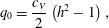
 $$\begin{eqnarray}\displaystyle & & \displaystyle \hspace{-24.0pt}(1+H)H_{t}=\frac{\unicode[STIX]{x2202}}{\unicode[STIX]{x2202}\unicode[STIX]{x1D703}}\left\{c_{V}\left(H+\frac{1}{2}H^{2}\right)-Re\,\frac{1}{3}H^{3}\cos \unicode[STIX]{x1D703}\right.\nonumber\\ \displaystyle & & \displaystyle \hspace{-24.0pt}\quad \left.+\,\left[\frac{H^{3}}{3Ca}\left(H_{\unicode[STIX]{x1D703}}+H_{\unicode[STIX]{x1D703}\unicode[STIX]{x1D703}\unicode[STIX]{x1D703}}\right)+\frac{1}{3}c_{V}^{2}ReH^{3}H_{\unicode[STIX]{x1D703}}-\frac{Re}{3}H^{3}H_{\unicode[STIX]{x1D703}}\sin \unicode[STIX]{x1D703}-\frac{Re}{2}H^{4}\cos \unicode[STIX]{x1D703}\right]\right\}.\end{eqnarray}$$
4 Results
In § 3, we derived four low-order models, related to one another as shown in figure 2:
(i) the ‘full’ long-wave model (2.7), (3.11) ( $\unicode[STIX]{x1D70E}_{LW}$);
(ii) the thin-film weighted residual model (3.13), (3.14) (
$\unicode[STIX]{x1D70E}_{TF}$);(iii) the long-wave gradient expansion model (3.18) (
$\unicode[STIX]{x1D70E}_{GR}$);(iv) the ‘classical’ thin-film gradient expansion model (3.19) (
$\unicode[STIX]{x1D70E}_{CL}$),


where the  $\unicode[STIX]{x1D70E}_{i}$ denote the growth rate of the most unstable linear mode of each model, respectively.
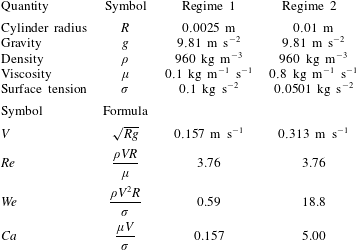
We validate the models against one another, as well as against direct numerical simulations of the full governing equations, in both the linear and nonlinear regimes, studied in §§ 4.1 and 4.2 respectively. It is found that only the full long-wave model provides consistently good agreement with the exact solutions across the considered parameter ranges. As a consequence, a combination of DNS and the long-wave model are used to map out parameter space in § 4.3. The problem is characterised by the four dimensionless groups  $Re,We,c_{R}$ and $c_{V}$ defined in (2.8); in order to investigate the corresponding four-dimensional parameter space we examine two different regimes as given in table 1. Both regimes have $Re=3.76$, which ensures that inertia is significant but not dominant, but differing Weber numbers. We then perform parametric studies by varying the rotation rate $c_{V}$ and the fluid mass $c_{R}$.
For high values of the rotation rate and/or fluid mass, the interface tends to become multivalued due to centrifugation and/or gravity respectively. This behaviour, which potentially includes dripping or other forms of rupture, is examined using DNS in § 4.3.3. Prior to the onset of this multivalued regime, the system exhibits either periodic or steady state behaviour, with lower rotation rates and greater fluid masses tending to favour steady states due to the dominance of gravitational effects. The steady states are examined in § 4.3.1, including parametric dependence on Reynolds number  $Re$ as well as the intricate limit point structures observed for low rotation rates by Lopes et al. (Reference Lopes, Thiele and Hazel2018). The periodic states show a complex variation of period and amplitude for increasing values of $c_{V}$. A characteristic example is studied in detail in § 4.3.2, including analysis of the bifurcations observed transitioning between regimes.
Dimensional variables corresponding to the two regimes examined here. Regime 2 is more easily realised physically but has too high a capillary number to observe some of the more unusual phenomena found in Regime 1.
4.1 Linear stability with no gravity
When the cylinder is spinning rapidly, or in a microgravity environment, the destabilising effect of the gravity is dominated by that of centrifugation (Evans et al. Reference Evans, Schwartz and Roy2004). In this case the gravitational effects may be neglected, and the system admits a base state with an interface of uniform thickness  $\bar{h}$. Computing the linear stability of this state is a useful mechanism for validating the models, as comparison with the exact solution is known to provide a stringent test: even in the absence of inertia, the one-equation models give poor predictions of the linear stability (Wray et al. Reference Wray, Matar and Papageorgiou2017a). In addition, this analysis allows us to isolate the importance of different physical mechanisms analytically, providing useful insight into the problem. In the absence of gravity, the velocity scaling $V=\sqrt{Rg}$ is no longer suitable; instead we scale based on the Reynolds number. In order to retain direct comparison with the other sections we allow $V$ to be defined by
 $$\begin{eqnarray}Re=\frac{\unicode[STIX]{x1D70C}VR}{\unicode[STIX]{x1D707}}=3.76.\end{eqnarray}$$
 For all low-order models we computed the stability of this state via a standard linearisation procedure about the base state, followed by a decomposition into normal modes of the form  $\text{e}^{\unicode[STIX]{x1D70E}t+\text{i}n\unicode[STIX]{x1D703}}$, so that $\unicode[STIX]{x1D70E}$ is the growth rate and $n$ is an integer wavenumber. For the two-equation models (the full long-wave model and the thin-film weighted residual model) the basic solution for the flux may be extracted by assuming both the height and the flux to be constant. We do not give explicit dispersion relations due to their comparative complexity.
To validate these results, we compare against a linearisation of the full governing equations. The corresponding basic state is
 $$\begin{eqnarray}u=0,\quad v=c_{V}r,\quad p=\frac{1}{We}\frac{1}{\bar{h}}+\frac{c_{V}^{2}}{2}(r^{2}-\bar{h}^{2}).\end{eqnarray}$$
 A streamfunction formulation for the perturbations followed by linearisation and decomposition into normal modes results in an Orr–Sommerfeld system that was solved using a Chebyshev–Tau algorithm (Dongarra, Straughan & Walker Reference Dongarra, Straughan and Walker1996). The most unstable mode is denoted by  $\unicode[STIX]{x1D70E}_{OS}$.
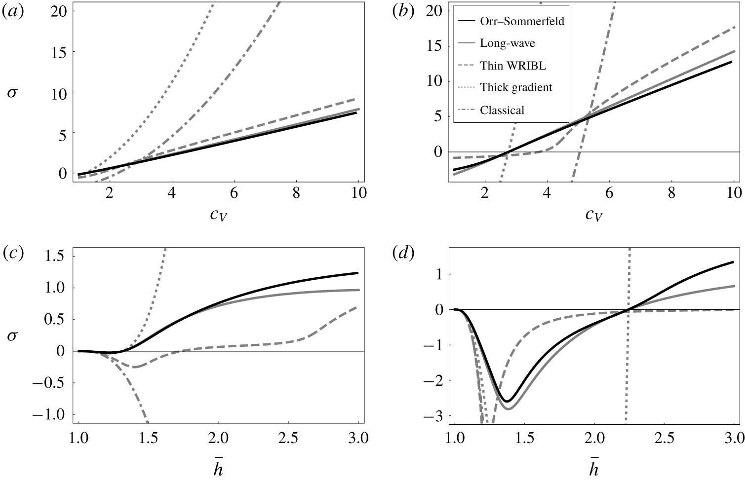
We look at both Regimes 1 and 2 from table 1 for  $n=2$ in figure 3, where Regime 1 is described by $We=0.59$ and Regime 2 by $We=18.8$. In general the long-wave model exhibits closest agreement with the Orr–Sommerfeld results, followed by the thin-film weighted residual model. The one-equation models (the thick-film gradient model and the classical model) exhibit strong disagreement with the Orr–Sommerfeld solution for all but the thinnest films at moderate rotation rates. All models correctly predict increasing growth rates for increasing values of $c_{V}$ due to the increased effect of centrifugation, although the one-equation models dramatically over-predict this effect. This will be analysed in detail shortly. Notably, for increasing values of $\bar{h}$ the Orr–Sommerfeld solution predicts a levelling in the growth rate, as previously observed by Wray et al. (Reference Wray, Papageorgiou and Matar2017b) in the absence of inertia. This again is better replicated by the two-equation models.
Growth rates as a function of rotation speed  $c_{V}$ and undisturbed interfacial radius $\bar{h}$ for $n=2$: (a) Regime 1; (b) Regime 2 from table 1.
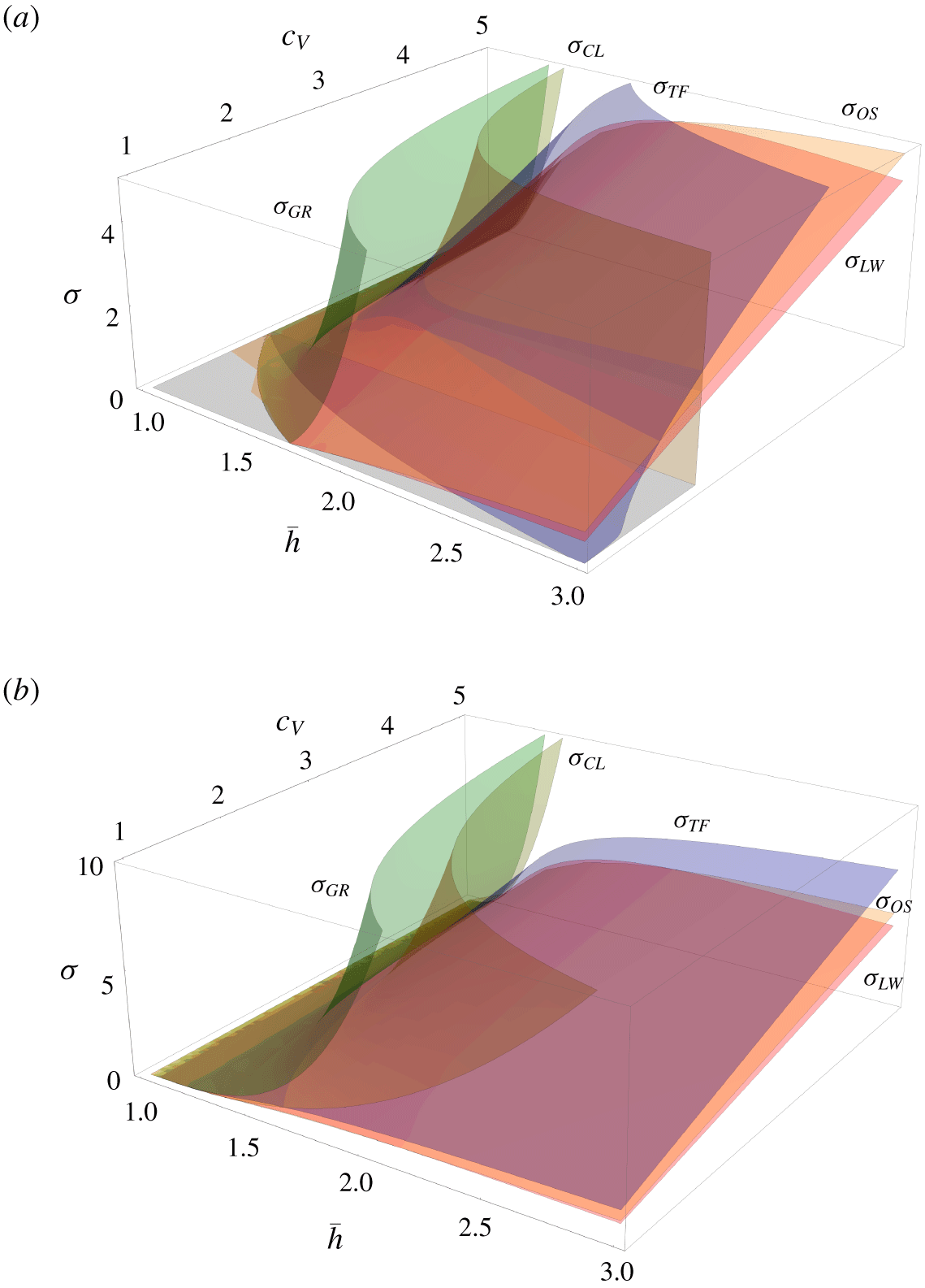
All models perform better in Regime 2. This is because this regime has a higher value of the Weber number, corresponding to weaker surface tension. The models are predicated on a leading-order solid-body rotational flow; the smaller the Weber number the greater the deviation from this and the worse the models perform. Similarly, for smaller values of  $c_{V}$ the rotational base flow is less dominant and so the agreement is weaker.
Of particular interest is the behaviour as  $c_{V}\rightarrow \infty$. For moderate $c_{V}$ the system is expected to be approximately in solid-body rotation, but for larger values of $c_{V}$ centrifugation dominates. Expanding the respective growth rates for large $c_{V}$ we find
 $$\begin{eqnarray}\displaystyle & \displaystyle \unicode[STIX]{x1D70E}_{CL}\sim \frac{(\bar{h}-1)^{3}}{3\bar{h}}n^{2}Re\,c_{V}^{2}+O(c_{V}), & \displaystyle \nonumber\\ \displaystyle & \displaystyle \unicode[STIX]{x1D70E}_{GR}\sim {\textstyle \frac{1}{8}}(\bar{h}^{4}-4\bar{h}^{2}\log (\bar{h})-1)n^{2}Re\,c_{V}^{2}+O(c_{V}), & \displaystyle \nonumber\\ \displaystyle & \displaystyle \unicode[STIX]{x1D70E}_{TF}\sim \frac{(\bar{h}+1)\sqrt{(1-\bar{h})\bar{h}((\bar{h}-14)\bar{h}-3)}}{2\bar{h}(5\bar{h}-1)}n\,c_{V}+O(1), & \displaystyle \nonumber\end{eqnarray}$$
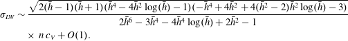 $$\begin{eqnarray}\displaystyle & & \displaystyle \displaystyle \unicode[STIX]{x1D70E}_{LW}\sim \frac{\sqrt{2(\bar{h}-1)(\bar{h}+1)(\bar{h}^{4}-4\bar{h}^{2}\log (\bar{h})-1)(-\bar{h}^{4}+4\bar{h}^{2}+4(\bar{h}^{2}-2)\bar{h}^{2}\log (\bar{h})-3)}}{2\bar{h}^{6}-3\bar{h}^{4}-4\bar{h}^{4}\log (\bar{h})+2\bar{h}^{2}-1}\nonumber\\ \displaystyle & & \displaystyle \phantom{\unicode[STIX]{x1D70E}_{LW}\sim }\times \,n\,c_{V}+O(1).\nonumber\end{eqnarray}$$
 In agreement with the Orr–Sommerfeld computations, the thin-film weighted residual and full long-wave model both correctly predict that the growth rate scales linearly with  $c_{V}$, whereas the one-equation models (the classical model and the long-wave gradient model) incorrectly predict that it scales quadratically with $c_{V}$. This is due to the way the respective models treat the physics of centrifugation. This effect enters primarily via the $-v^{2}/r$ term in the $r$-momentum equation (2.2). In a film flow such as the present one, this manifests as a disturbance to the pressure as observed in (3.2). It therefore enters the system as an adjustment to the streamwise velocity, or in this low-order formulation, the flux. Thus it should be treated as a dynamic wave, with the primary balance being between the rate of change of the streamwise velocity $v_{t}$ and the pressure gradient, resulting in the growth rate scaling with $c_{V}$. Similarly, as $v_{t}$ scales with the azimuthal gradient of the pressure, the two-equation models correctly predict a linear dependence on the wavenumber $n$. In the one-equation formulations, the slaving of the flux to the height erroneously forces this centrifugation to enter via a kinematic wave, resulting in the incorrect dependence on both $n$ and $c_{V}$. Note that this also spuriously results in the expressions for the one-equation models depending on the Reynolds number. The final observation of interest is that as the rotation rate increases the most unstable mode will actually increase – this is related to the observation of Evans et al. (Reference Evans, Schwartz and Roy2004) of an increasing cutoff wavenumber for increasing rotation rate.
Growth rates corresponding to Regime 1 in table 1. (a,b) Effect of varying  $c_{V}$ for $\bar{h}=1.5$; (a) $n=2$, (b) $n=4$. (c,d) Effect of varying $\bar{h}$ for $c_{V}=1.5$; (c) $n=2$, (d) $n=4$.
We look in more detail at some characteristic cases in figure 4. In particular, for Regime 1 we examine the effect of varying  $c_{V}$ for a fixed $\bar{h}$ (a,b), and of varying $\bar{h}$ for a fixed $c_{V}$ (c,d), for both $n=2$ (a,c) and $n=4$ (b,d). In the top row we see the anticipated dependence on $c_{V}$ and $n$ playing out: for the one-equation models the growth rate scales quadratically with the rotation rate $c_{V}$ whereas the two-equation models (correctly) exhibit a linear scaling. What is more, the gradient of the lines for the two-equation models scale with $n$ so that the gradient of the growth rates in (b) is approximately double that in $(a)$.
In the second row we see the behaviour with varying  $\bar{h}$. In particular, this elucidates the $\bar{h}-1\ll 1$ region omitted in figure 3(a) as it falls outside the plotting region. For small values of $\bar{h}$, capillarity dominates, stabilising the flow. Note that this effect is stronger in (d) as this corresponds to a higher value of the wavenumber ( $n=4$) resulting in a stronger stabilising effect. For increasing values of $\bar{h}$ more fluid is further away from the axis of rotation, resulting in a stronger effect of centrifugation. This effect eventually dominates and results in instabilities. Of interest is the levelling behaviour observed for the largest values of $\bar{h}$; this is an effect that the one-equation models fail to pick up, satisfying power laws ( $\unicode[STIX]{x1D70E}_{CL}\sim \bar{h}^{2},\unicode[STIX]{x1D70E}_{GR}\sim \bar{h}^{4}$). In particular, for the classical linear stability the coefficient is even of the wrong sign, predicting successively greater decay rates for increasing $\bar{h}$. This failure is natural, however: in this region the terms neglected due to their azimuthal derivatives are more important, and the treatment of all disturbances as kinematic waves in the one-equation models becomes successively less valid.
4.2 Nonlinear validation
In order to provide additional insight into the properties of the previously discussed reduced-order methodologies, we wish to validate the models against the results of the DNS. We again use the two regimes given in table 1. In each of these, we can now perform a parametric study on the two remaining parameters: the rotational speed of the disc  $c_{V}$ and the initial radius of the fluid $c_{R}$. We mapped out parameter space using transient computations as described in appendix A.1. Note that the current modelling method cannot track the interface into a multivalued regime due to our parameterisation by the azimuthal angle $\unicode[STIX]{x1D703}$. In addition, at this threshold the interfacial slopes are so large that the long-wave reduction is no longer valid. However, there may be other parametrisations that afford continuation beyond this point. Bezier curves were fitted to the transition boundaries as plotted in figure 5. The steady/periodic boundary observed for Regime 1 was also validated using path continuation as described in appendix A.2. Direct numerical simulations (expanded upon in appendix A.3) were performed along the identified transition boundaries to validate the predictions of the long-wave model – the results of these computations are given as symbols in figure 5.
In light of the good observed agreement, we will defer detailed investigation of the long-wave model to § 4.3, and instead examine the accuracy of the other models. In figure 6 we compare the four models for two parameter regimes. Videos of these two scenarios are included as Movie 1 and Movie 2 in the supplementary material available at https://doi.org/10.1017/jfm.2020.421.
4.2.1 Low speed, thick flow: $c_{V}=0.5,c_{R}=1.5$.

In figure 6(a) we see the behaviours of the models for  $c_{V}=0.5$, $c_{R}=1.5$. These parameters correspond to a relatively thick flow at a moderate rotation speed. Note that although initially the thickness of the liquid layer is only half the radius of the fibre, the accumulation of the liquid into a hanging drop rapidly results in a situation where the system is significantly thicker (the maximal radius of the long-wave model at steady state is approximately $2.53$).
Parametric studies in  $c_{V}$ and $c_{R}$ for both (a) Regime 1 and (b) Regime 2 as given in table 1. Solid black lines correspond to delineations between flow regimes as predicted by the long-wave model. Symbols correspond to DNS results, with squares representing steady states, circles representing (temporally) periodic states and diamonds representing situations where the interface becomes multivalued.
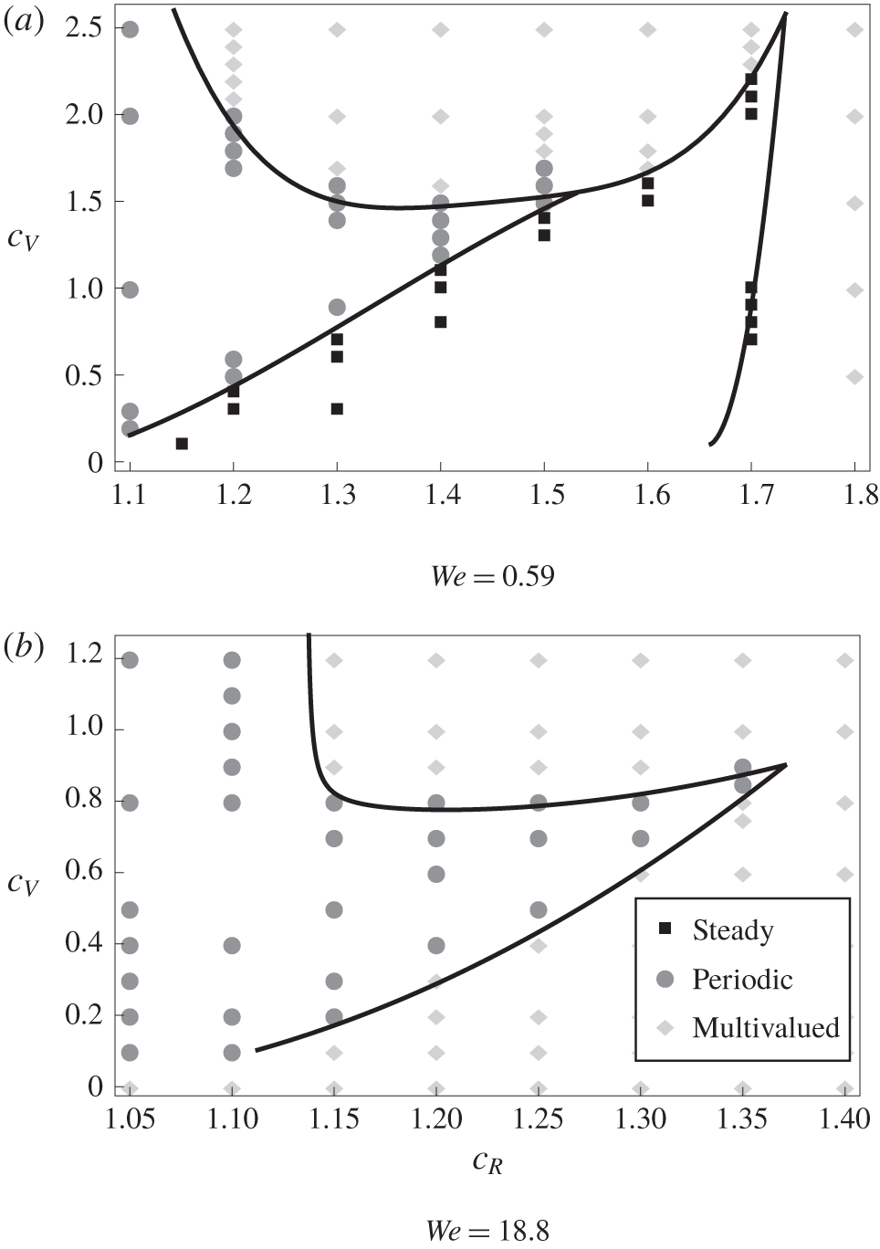
As might reasonably be expected, the steady states for the thin-film models match one another quite well, as do those for the thick-film models; however, these two sets of predictions differ quite strongly from one another, with the thin-film models predicting rather more compact drops, with centres of mass closer to the origin.
However, despite the good steady state agreement for the two thick-film models, we see significant discrepancies in their transient behaviours. The full model shows a notable swing in the positive  $\unicode[STIX]{x1D703}$ direction, followed by a settling back (in agreement with the DNS), while the movement of the centre of mass for the long-wave gradient model is almost monotonic. By contrast, while the thin-film weighted residual model ultimately predicts a significantly incorrect final interfacial shape, it agrees quite well with the long-wave model in early-time behaviour. This is because the observed initial overshoot and settling back is an inertial effect: as a result models using the weighted residual method perform significantly better as the velocity has its own independent field $q$.
$q$.
4.2.2 Moderate speed, thick flow: $c_{V}=1,c_{R}=1.5$

The agreement between the predicted steady states for the full long-wave model and the long-wave gradient model is significantly worse than in the previous case. To elucidate why this discrepancy has occurred, we consider the predicted interfacial shapes for steady states by setting  $\unicode[STIX]{x2202}_{t}=0$ in (2.7), (3.11) and (3.18). The kinematic condition for the full problem (2.7) tells us that the flux $q$ is constant. As a result the balance between capillarity, gravity, constant flux and solid-body rotation flow in the first line of (3.11) is identical to that in the corresponding terms in the right-hand side of the long-wave gradient model (3.18). Thus the only differences are the second order viscous terms on the second line of (3.11), and the inertial terms. The former has not been significant in other contexts, and indeed a quick numerical computation (not presented here) shows that it is not the culprit for the inconsistency: in fact it is purely the treatment of the inertial terms. With $c_{V}=1$ the inertial terms in the gradient expansions scale as $Re\,c_{V}^{2}=3.76$, which is sufficient to cause strong disagreement between the models.
Comparison between the various reduced-order models. Analytical results are shown as a solid, blue line for the full long-wave model (2.7), (3.11); a dashed, green line for the thin-film weighted residual model (3.13), (3.14); a dotted, yellow line for the thick-film gradient model (3.18); a dash-dotted red line for the thin-film gradient (Kelmanson) model (3.19). The black lines correspond to DNS results. The closed loops correspond to the final interfacial shapes. The lines emanating from the centre correspond to the centres of mass of the liquid over time in the respective simulations, while the lines starting further down the  $y$-axis correspond to the points of maximal interfacial radius over time. Animations of these comparisons are provided as Movie 1 and Movie 2 respectively in the supplementary material.
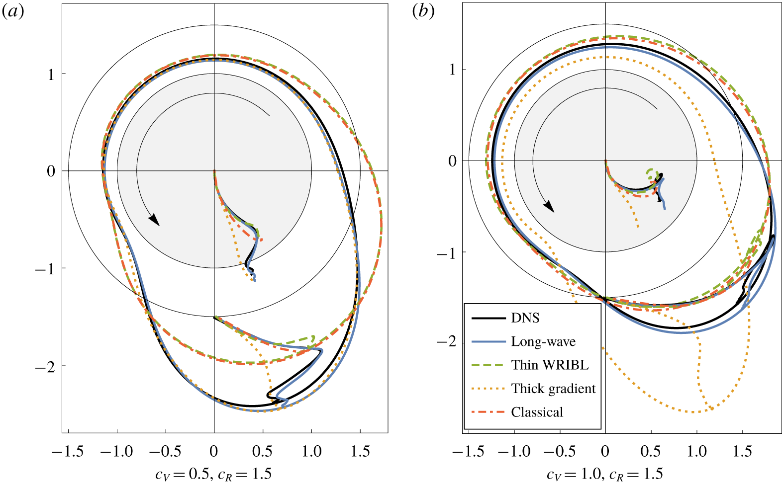
Once again the thin-film weighted residual model performs reasonably well at early times, correctly capturing the inertial behaviour, but fails to predict the final interfacial shape. We thus see that, despite its comparative complexity, the careful treatment of both geometric and inertial effects required to produce the long-wave weighted residual system (2.7), (3.11) is essential to the production of a viable model.
4.3 Parametric study
The phase planes given in figure 5 demonstrate a wide variety of possible behaviours. As noted in the introduction, the left-hand side of these planes, corresponding to thin-film solutions, have already been extensively studied. We therefore concentrate on the more complex behaviours shown by thicker flows, examining them in detail using both DNS and the long-wave equations.
4.3.1 Steady states
One distinct difference between Regime 1 and Regime 2 is that the latter does not exhibit (stable) steady states. This is due to the weaker surface tension. Nonetheless, a significant amount of liquid can be held on the surface of the cylinder by rotating it sufficiently quickly, but in Regime 2 this always results in a periodic state. In order to compute the steady states observed in Regime 1, we set  $\unicode[STIX]{x2202}_{t}\mapsto 0$ so that the kinematic condition (2.7) indicates the flux is some constant $q_{0}$, while (3.11) becomes
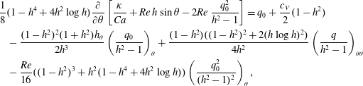 $$\begin{eqnarray}\displaystyle & & \displaystyle \frac{1}{8}(1-h^{4}+4h^{2}\log h)\frac{\unicode[STIX]{x2202}}{\unicode[STIX]{x2202}\unicode[STIX]{x1D703}}\left[\frac{\unicode[STIX]{x1D705}}{Ca}+Re\,h\sin \unicode[STIX]{x1D703}-2Re\,\frac{q_{0}^{2}}{h^{2}-1}\right]=q_{0}+\frac{c_{V}}{2}(1-h^{2})\nonumber\\ \displaystyle & & \displaystyle \quad -\,\frac{(1-h^{2})^{2}(1+h^{2})h_{\unicode[STIX]{x1D703}}}{2h^{3}}\left(\frac{q_{0}}{h^{2}-1}\right)_{\unicode[STIX]{x1D703}}+\frac{(1-h^{2})((1-h^{2})^{2}+2(h\log h)^{2})}{4h^{2}}\left(\frac{q}{h^{2}-1}\right)_{\unicode[STIX]{x1D703}\unicode[STIX]{x1D703}}\nonumber\\ \displaystyle & & \displaystyle \quad -\,\frac{Re}{16}((1-h^{2})^{3}+h^{2}(1-h^{4}+4h^{2}\log h))\left(\frac{q_{0}^{2}}{(h^{2}-1)^{2}}\right)_{\unicode[STIX]{x1D703}},\end{eqnarray}$$
 where  $q_{0}$ may be determined by imposing mass conservation. We can then trace out solution branches in parameter space using pseudo arc-length continuation as described in appendix A.2. The branches can be continued into regions where they are unsteady, with the linear stability being checked by the computation of the corresponding generalised eigenvalue problem. In particular, we find that the steady-to-periodic transition in Regime 1 occurs via a supercritical Hopf bifurcation, with a complex conjugate pair of eigenvalues crossing the imaginary axis with non-zero velocity. In general the periodic disturbance will manifest as a small surface wave travelling around the interface of the previously steady drop.
The steady states of the zero Reynolds number problem have recently been examined in detail by Lopes et al. (Reference Lopes, Thiele and Hazel2018), comparing a variety of low-order models against a finite-element-based Stokes solver. Following their exposition in order to compare results, we map our solutions in parameter space against the perimeter length of the flow, denoted by  $s$.
$s$.
Low inertia limit
Lopes et al. (Reference Lopes, Thiele and Hazel2018) observed that for certain parameter regimes there was a multiplicity of solutions, with up to four solutions being observed for some parameter sets. In order to compare against their results, which neglected inertia, we discard all inertial terms in (4.3) (i.e. all those multiplied by  $Re$ save the gravitational term $Re\,h\sin \unicode[STIX]{x1D703}$, where we set $Re=1$) and use a fixed volume of $0.21\unicode[STIX]{x03C0}$, which corresponds to a film thickness of 0.1 in an undisturbed state. Such thin films at moderate rotation rate exhibit a solution with near-uniform thickness where capillarity is negligible so that gravity and rotational effects dominate. These solutions have a maximum at $\unicode[STIX]{x1D703}\approx 0$ where rotation and drainage act in opposition to one another, and a minimum at $\unicode[STIX]{x1D703}\approx \unicode[STIX]{x03C0}$ where they work in concert. Such solutions correspond to the classical steady solution observed by O‘Brien & Gath (Reference O‘Brien and Gath1998). As a result we initialise our calculations at $c_{V}=3$ using constant thickness as an initial guess, and trace out our branches from there. The results are given in figure 7 for $Ca\in \{2,6,10,14,18\}$.
Parametric study of the steady states of (4.3) in the absence of inertia. Rotation rate  $c_{V}$ is plotted against dimensionless fluid perimeter $s$. (a) Parametric steady state study for $Ca\in \{2,6,10,14,18\}$. The arrow indicates the direction of increasing $Ca$. (b) Detail of boxed region for $Ca=14$ demonstrating the multiplicity of solutions. (c) Interface profiles corresponding to the multiple indicated solutions.
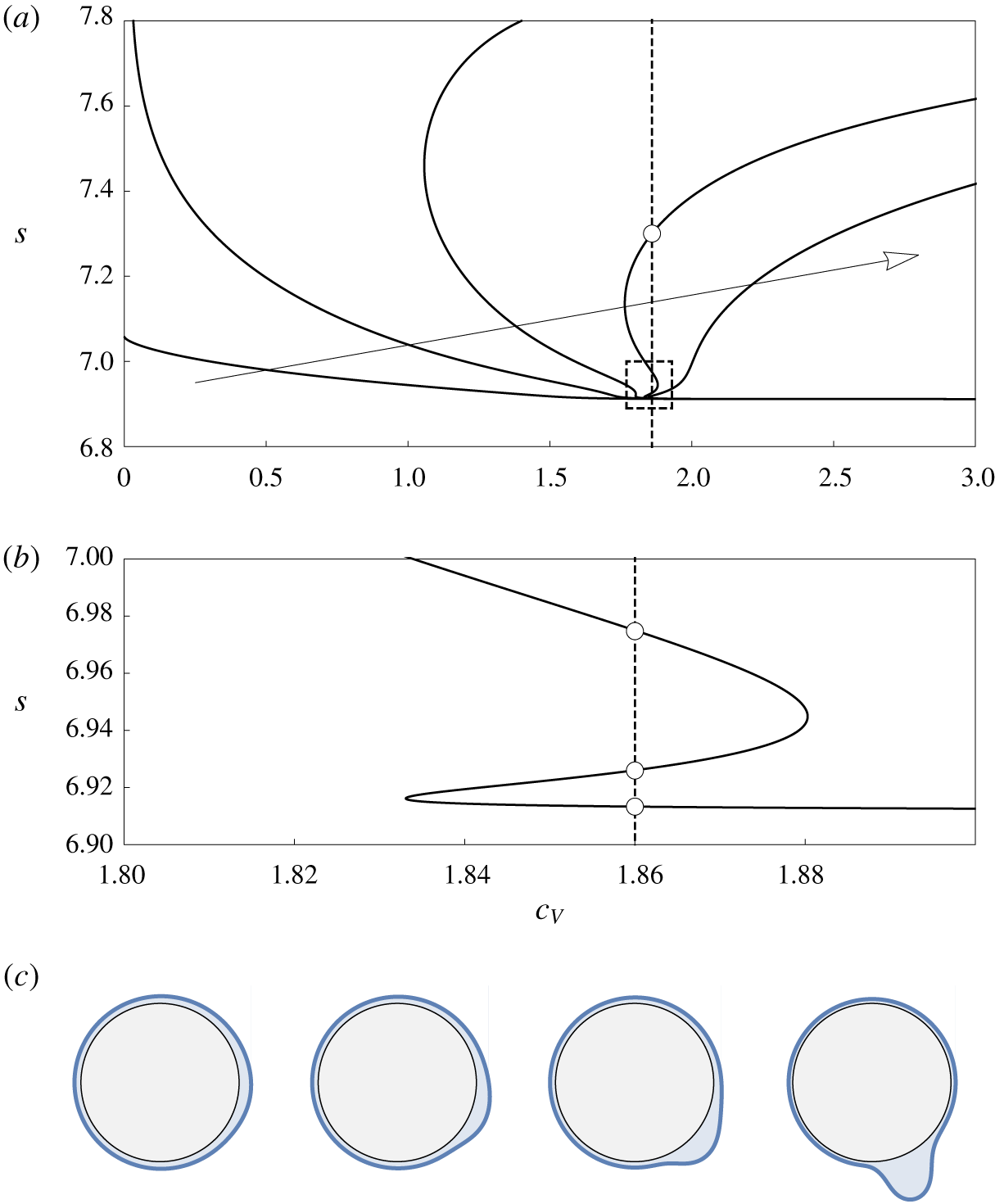
Parametric study on the effect of the Reynolds  $Re$ for $Ca=0.157,c_{V}=0.5$ and $c_{R}\in \{1.3,1.4,1.5,1.6\}$. Dashed lines indicate long-wave results (4.3) while the solid lines corresponds to DNS calculations. (a) Dimensionless fluid perimeter $s$ versus Reynolds number. The arrow indicates the direction of increasing $c_{R}$. (b) Interfaces corresponding to $Re=9,7,5,3$ for $c_{R}=1.3,1.4,1.5,1.6$ respectively from left to right, as indicated by the circles on the upper image.
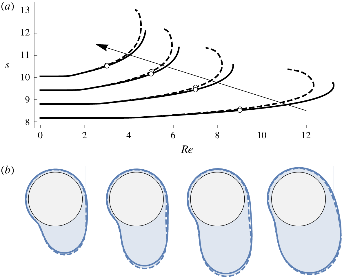
As observed by Lopes et al. (Reference Lopes, Thiele and Hazel2018), for small values of  $Ca$ surface tension dominates and only a single solution is exhibited. As $Ca$ is increased (corresponding to gravity being successively more significant relative to capillarity) a limit point develops corresponding to the loss of the pendant-drop solution, and for higher values of $Ca$ at least two solutions are observed with the upper branch being unstable. They noted that the formation of this first limit point is only recovered by models incorporating the full expression for the curvature: the approximated curvature of the classical models leads to too inaccurate a formulation of the hydrostatic pressure balance.
For even larger values of  $Ca$, Lopes et al. observe parameter ranges exhibiting four distinct solutions. While this phenomenon is not captured by any of their low-order models, the long-wave model (4.3) appears to capture it effectively as shown in figure 7(b,c). These solutions are lost when the second-order viscous terms given on the second line of (4.3) are removed. Therefore, despite the comparative complexity of these terms, it appears important to retain them in order to provide good agreement with the intricacies of the exact solutions. However, the branches of the long-wave model exhibiting four solutions correspond to slightly higher values of $Ca$ than those observed by Lopes et al.: for their inset $Ca=20$, whereas for ours $Ca=14$. We suspect this is because of the comparatively simple nature of our projection polynomials for our velocity profiles. In particular, at leading order our solution is simply solid-body rotation (3.7). This simple linear profile exhibits no deformation of fluid elements. As a result, both at leading order and higher orders (for which the profiles are based on the leading-order profile (Ruyer-Quil & Manneville Reference Ruyer-Quil and Manneville2000; Benilov & O’Brien Reference Benilov and O’Brien2005)), the flow is likely to underpredict the deformation of fluid elements, corresponding to an underprediction of viscous energy dissipation, i.e. the value of the second-order viscous dissipation terms is likely to be erroneously small. This causes an imprecision in the balance between capillarity, viscosity and gravity, causing the triple limit point structure to occur for an incorrect value of $Ca$. We anticipate that this underprediction of the rate of viscous dissipation could conceivably be rectified by allowing for the flow to be driven by a combination of solid-body rotation and capillarity at leading order, at the cost of severely complicating the model.
Inertial effects
Returning to the full steady equation (4.3), we examine the effect of the Reynolds number in figure 8 for  $Ca=0.157,c_{V}=0.5$. For small values of $Re$ there is a near-uniform base state. We therefore initialise our calculations with $Re=10^{-6}$ and an initial guess of a uniform state. We then trace out branches for an initially increasing Reynolds number. We use volumes corresponding to a base state with $c_{R}\in \{1.3,1.4,1.5,1.6\}$. In order to validate our solutions we also directly compute numerical solutions of the steady Navier–Stokes equations. This was done using a standard remapping of the physical domain onto a rectangular computational domain, together with numerical path continuation as described in appendix A.2. All branches are only continued as far as can be reliably resolved: in each case the interface eventually becomes multivalued, at which point they cannot be tracked using this mechanism. Thus, while the Navier–Stokes solver can in principle compute past limit points, we cease tracing the branches once the interface is no longer single valued which, for these particular parameters, is in the vicinity of the observed limit points.
In this non-dimensionalisation, increasing the Reynolds number for a fixed Capillary number corresponds to increasing the Weber number, so that the relative significance of gravity compared to surface tension increases. Thus for small Reynolds numbers, capillarity dominates so that the interface is nearly circular. As the Reynolds number increases, gravity becomes more significant and the interface deviates further from circularity, resulting in a greater value of the fluid perimeter  $s$. Again it appears that there is a limit point, however, the branches cannot be continued past this point as the interface becomes multivalued close to this point and the respective methods break down.
For each value of  $c_{R}$ a corresponding interface is plotted for an appropriate Reynolds number in figure 8(b). Across these interfaces the maximum interfacial position is in error by at most $4.18\%$ for $c_{R}=1.4$, $Re=7$ where long-wave theory predicts a maximum interfacial radius of $2.60$ as opposed to $2.49$ for the DNS. This indicates that even for films with radii multiple times the radius of the disk good predictive agreement is achieved.
4.3.2 Periodic behaviour
It is clear that, especially for very thin films, solid-body rotation behaviour dominates (the right-hand side of (3.19) is dominated by the lowest power of  $H$, due to the convective term). Indeed, for such thin films the period of these states would be expected to be close to the period of the rotation of the disk $T_{D}=2\unicode[STIX]{x03C0}/c_{V}$. For slightly thicker films, a delicate interplay of multiple time scales arises (Hinch & Kelmanson Reference Hinch and Kelmanson2003; Kelmanson Reference Kelmanson2009). We now examine the periodic behaviour of a film across a wide variety of thicknesses. Based on figure 5(b) we examine the period $T$ and maximal amplitude $A$ of flows in Regime 2 for $c_{V}=0.7$ for a variety of initial thicknesses, as shown in figure 9. This was computed by performing transient simulations for successively larger values of $c_{R}$ starting at $c_{R}=1.05$. The final configuration for a given value of $c_{R}$ was used as the initial condition for the subsequent value.
Transient computations of time-periodic solutions using the full long-wave model (2.7), (3.11) for  $Re=3.76,Ca=5,c_{V}=0.7$. (a) Time period $T$ and maximal amplitude $A$ of the periodic solutions for varying values of $c_{R}$; (b) space–time plots for $c_{R}=1.1$ (left) and $1.2$ (right), decomposed as (4.4) (with $\tilde{h}$ being plotted); (c) characteristic interfacial shapes for $c_{R}=1.2$ for the draining phase (left) and inertia–capillarity phase (centre). Right: the streamlines when the base flow $v=c_{V}r$ is subtracted off, demonstrating the draining behaviour.
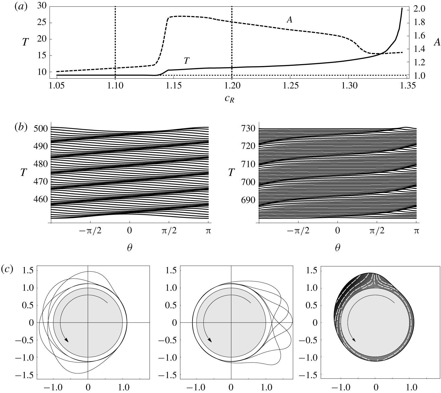
It is seen from figure 9(a) that for  $c_{R}\lesssim 1.13$ the period of the solution is very close to $T_{D}$ (denoted by the horizontal dotted line). However, this changes more rapidly thereafter so that by $c_{R}=1.175$ the period has increased by 24%. This transition lies outside the range of anticipated applicability of thin-film models (Wray et al. (Reference Wray, Papageorgiou and Matar2017b) found that, at least according to linear theory, the results of thin-film models could not be trusted once $c_{R}$ exceeded 1.1). The time period continues to increase monotonically so that, by $c_{R}=1.345$, it reaches a value of $2.992T_{D}$. The period does not diverge, however, and, as in Regime 1, the system experiences a supercritical Hopf bifurcation. In this scenario, this occurs at $c_{R}=1.346$, with stable steady states being recovered for larger values of $c_{R}$ (verified by both transient computations and checking the eigenvalues of the linear stability of the steady state). There is a narrow band of steady states where the interface remains single valued, $1.346\lesssim c_{R}\lesssim 1.347$, after which the interface becomes multivalued. Note that this band is not picked up in the parametric study, not due to insufficient search resolution, but because in the respective study the interface was always started from a uniform initial thickness and zero flux.
In figure 9(b) we examine the spatio-temporal evolution of the periodic behaviour for  $c_{R}=1.1$ (left) and $c_{R}=1.2$ (right). In order to elucidate the behaviour we decompose
 $$\begin{eqnarray}h=\bar{h}(\unicode[STIX]{x1D703})+\tilde{h}(\unicode[STIX]{x1D703},t),\end{eqnarray}$$
where
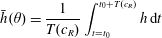 $$\begin{eqnarray}\bar{h}(\unicode[STIX]{x1D703})=\frac{1}{T(c_{R})}\int _{t=t_{0}}^{t_{0}+T(c_{R})}h\,\text{d}t\end{eqnarray}$$
 is the period-averaged behaviour of  $h$, with $t_{0}$ chosen sufficiently large as to discard any initial transient into the periodic motion. Thus $\tilde{h}$ is the deviation of $h$ from its cycle-averaged value. For $c_{R}=1.1$ the disturbance $\tilde{h}$ is essentially a sinusoidal wave propagating around at uniform speed, as expected. For $c_{R}=1.2$ a much more localised coherent structure is formed. Its speed also varies noticeably across a single period.
In order to explain in more detail what is happening for  $c_{R}>1.13$, we plot the interfaces during the two ‘phases’ of one period for $c_{R}=1.2$ in figure 9(c). The left-hand image represents the first half of the period while the central one represents the second half. On the left-hand side a bulge of fluid is present at the highest point of the disk, but has little inertia. As a result, the drop essentially drains vertically down to the bottom, albeit predominantly on the left-hand side due to the rotation of the disk. This is highlighted on the right-hand side of (c) where we plot the streamlines as found when the background flow $v=c_{V}r$ is subtracted off: as can be seen the additional flow is essentially a draining flow under gravity. During this draining, the liquid gains kinetic energy due to the rotation of the disk and the conversion of gravitational potential energy. This manifests as a rapid swing to the right-hand side of the disk as shown in the second phase. In the first phase, the main competition was between gravity and viscosity; in this second phase, the more rapid swing results in an increased significance of inertia (in particular centrifugation), which is balanced by surface tension. The drop is swung up to the top of the disk, with the energy again converted into gravitational potential energy, so that the oscillation repeats.
We note that this is one of the most complex regions of phase space, with a complete description of the dynamics involving the interplay of viscosity, inertia, gravity and surface tension. Moreover, at the key point where gravity-induced draining starts to dominate, the layer is quite thick, and thus the deviation of the velocity profile from parabolic most significant, so that a complete model also relies crucially on accurate modelling of a ‘thick’ layer.
4.3.3 Multivalued states
For sufficiently large film thickness  $c_{R}$ and/or rotation speed $c_{V}$ the interface always eventually becomes multivalued. The modelling framework described in the previous subsections cannot characterise such events, however, these types of regimes are well captured via DNS, allowing us to inspect the break-up dynamics in detail.
Snapshots of two cases of interfacial break-up, with parameters as in Regime 1 given in table 1. In case (a) this is achieved by the fluid mass slowly draining on the outside of the inert cylinder, while in case (b) strong rotational movement determines centrifugal rupture.
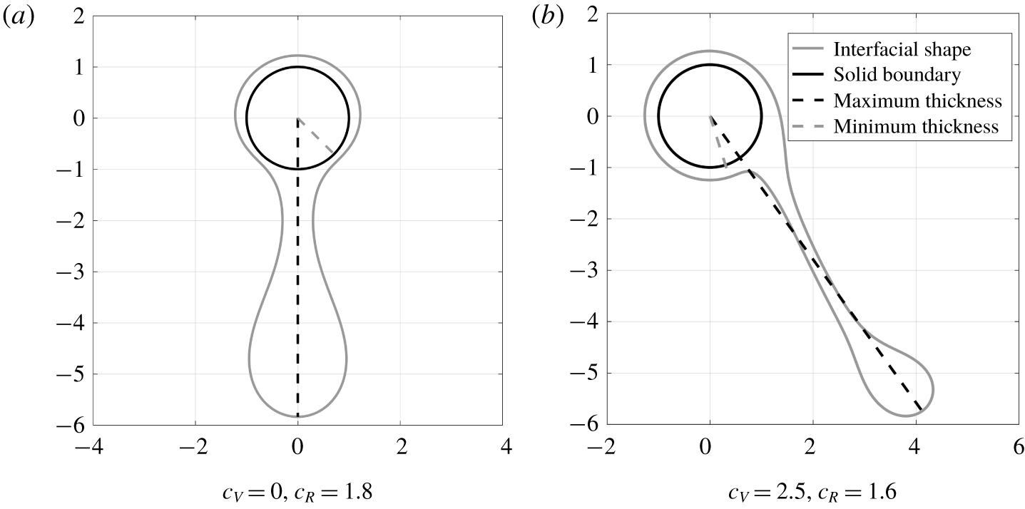
(a) Time evolution of minimum and maximum interfacial thickness  $(h-1)$ during the DNS for $c_{V}=1.9,~c_{R}=1.5$ in Regime 1, with the remaining parameters provided in table 1. (b) Interfacial shape and norm of the velocity field restricted to the liquid phase as extracted at the final time step illustrated on the left-hand side. Representative streamlines decorated with arrows indicating the direction of the flow and thick lines indicating the points of minimum (grey) and maximum (black) thickness are also plotted. An animation of this flow regime is included as Movie 3 in the supplementary material.
For all scenarios presented below, we refer back to what we call Regime 1 in table 1, with the behaviour diagram shown in figure 5(a). The lower  $Ca$ regime is considerably richer and has allowed the identification of several unanticipated configurations. Before analysing these, however, we mention that there are two expected transitions to multivalued states that are cleanly captured and shown in figure 10. For sufficiently large values of $c_{R}$ (here above $1.7$) and sufficiently low values of $c_{V}$ (starting from a stationary cylinder) gravity is the dominant force, with the mass of fluid simply slowly draining around the cylinder. Eventually the heavy fluid mass below the cylinder is enough to transition into a state with a quickly growing and thinning fluid filament drawn downward by a heavy pendant drop, causing eventual break-up. Quantitative aspects of this process are of course heavily dependent on the parameter values and would arguably be better analysed in a three-dimensional setting, but they are nevertheless a relevant feature at the limit of our parameter space. The other distinguished case is illustrated in figure 10(b), where usually within one rotation cycle a large fluid mass is quickly swung around the cylinder, now with centrifugation as the critical mechanism encouraging break-up, however, with gravity accentuating the movement of the fluid mass further away from the cylinder. It should be noted that interfacial rupture itself may not occur until after several time units, with the observed dynamics encouraging the search for periodic states. Such a case is identified and described in figure 11. In a regime of intermediate values of $c_{R}=1.5$ and $c_{V}=1.9$, just beyond what the model captures as periodic states, we find that, after a strong initial deformation into a number of thick fluid regions, there is a subtle interplay between (typically) two fluid masses, which, based on numerical evidence, is capable of sustaining itself indefinitely. This behaviour is specific to several tested configurations in this region of the parameter space and appears to be closely related to the multi-modal interactions observed by Groh & Kelmanson (Reference Groh and Kelmanson2014). At each moment in time (after a transient) the state itself is multivalued, however, rupture does not occur. In fact, this scenario is quite similar to the case detailed on in previous § 4.3.2, illustrated in figure 9. Whereas before the same fluid mass was oscillating between two phases: a gravity–viscous regime on the left-hand side of the motion, followed by a rapid swing and an inertial–capillary regime on the right-hand side of the disk, in the present case two roughly equal fluid masses undergo this type of motion at the same time, with each one finding itself in one of the two phases mentioned above and the overall dynamics reaching a well-ordered time-periodic behaviour. Pushing $c_{V}$ even further leads to immediate instability growth and violent rupture even within a single rotation cycle, with such cases being a considerable challenge in terms of gaining quantitative understanding.
Another interesting case is illustrated in figure 12, in which a large fluid mass with  $c_{R}=1.8$ is rotated very quickly with $c_{V}=3.0$, a regime towards the far top right corner of the behaviour diagram in figure 5(a). For lower values of $c_{V}$ the fluid is easily pulled down by gravity and ruptures within the initial movement cycle. Beyond a certain critical threshold, however, which here we find to be $c_{V}\approx 2.5$, centrifugation becomes a sufficiently relevant stabilising mechanism to overcome this. The fast flow in the immediate vicinity of the cylinder becomes strong enough to prevent further thinning (thus hampering more of the liquid mass from entering the main lobe) and the flow evolves to a steady state which in itself is actually not multivalued. The quasi solid-body rotation around the cylinder itself is counteracted by a large counter-rotating vortex inside the main lobe. Such a final state could in theory be captured by the reduced-order model, however, the transient multivaluedness in the first rotation precludes the identification of this regime using the equations in question.
(a) Time evolution of minimum and maximum interfacial thickness  $(h-1)$ during the DNS for $c_{V}=3.0,~c_{R}=1.8$ in Regime 1, with the remaining parameters provided in table 1. (b) Interfacial shape and norm of the velocity field restricted to the liquid phase as extracted at the final time step illustrated on the left-hand side. Representative streamlines decorated with arrows indicating the direction of the flow and thick lines indicating the points of minimum (grey) and maximum (black) thickness are also plotted. An animation of this flow regime is included as Movie 4 in the supplementary material.
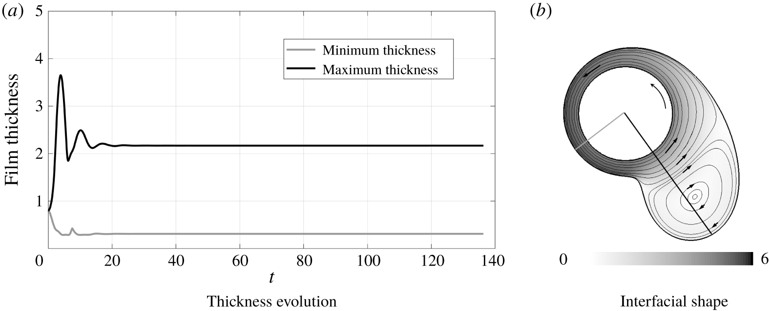
The multitude of scenarios presented above throughout § 4 form a rich and sometimes unexpected range of behaviours. This could only be constructed through an efficient identification of the regime boundaries using the newly developed model, informing the more accurate and more versatile – but much more expensive – direct numerical explorations of the target regimes. For example the two concrete families of solutions discussed in the present subsection (time-periodic multivalued and transiently multivalued converging to steady states) occupy a relatively small region inside the vast multi-dimensional parameter space of the problem. It is envisioned that a hierarchical approach would be undertaken in the case of assisting experimental and application-based studies, in which initially model results inform high-accuracy simulations towards regions of interest, which can subsequently be examined in a laboratory setting. The theoretical approaches could then complement experiments in terms of providing quantities inside the flow which would be challenging to image and/or measure.
4.4 Modelling discussion
The modelling of flows over substrates which are curved in the streamwise direction raises a number of interesting points. As a preliminary, we note that the method of weighted residuals relies critically on the determination of the projection polynomials (in fact only the leading order one is necessary for the ‘simplified’ model (Scheid et al. Reference Scheid, Ruyer-Quil and Manneville2006)), but the subsequent derivation is essentially agnostic of the physical mechanism driving it. For example, in the planar derivation of Ruyer-Quil & Manneville (Reference Ruyer-Quil and Manneville2000), if one switched the order of gravity and capillarity (which in their derivation are leading and first order respectively), the final model would actually be identical. This is because both would drive a parabolic flow at leading order – thereafter the projection method proceeds independently of whether it was gravity or capillarity driving at leading order; it relies only on the form of the polynomial. This is in stark contrast to a gradient expansion where the determination of higher-order terms in the asymptotic expansion would result in higher-order derivatives of the leading-order mechanism – a rather simpler proposition for gravity than for capillarity. This also has an interesting ramification for  $c_{V}$: implicit in the derivation of the one-equation models (3.18), (3.19) is that $c_{V}$ is constant. If $c_{V}$ were allowed to vary as a function of time this would significantly complicate these one-equation models, but would leave the two-equation models unaffected.
It is a peculiarity of (quasi-)planar geometries that the polynomials corresponding to body forces and to pressure gradients coincide. Indeed for thin-film flows, a substrate locally appears flat at leading order, and so both body forces and pressure gradients give rise to parabolic profiles. However, the (far more physically common) situation of thick flows on curved substrates exhibits rather different phenomena. Indeed, if the substrate is curved in the streamwise direction the two polynomials will in general not coincide (Wray et al. Reference Wray, Matar and Papageorgiou2017a). This renders the determination of the leading-order polynomial a matter of more care and importance. What is more, this polynomial has a significant impact on the complexity of the resulting model. In the present work we have chosen a situation where the leading-order flow is driven neither by gravity nor by a pressure gradient but rather by rotation of the substrate. As a result the leading-order polynomial is actually the simple monomial  $v\propto r$; this is what accounts for the fact that the resulting model (3.11) is actually (comparatively) simple. And yet despite this rather straightforward approximation the model has performed quite well.
The above being said, the selection of the leading-order flow as being solid-body rotation might limit the model’s range of validity. In particular, this leading-order solution is not a true flow: there is no deformation of fluid elements; in the frame of reference moving with the disk the flow is not simply steady but actually stationary. It might therefore be more suitable to decompose the flow as  $v=c_{V}r+\tilde{v}$, taking $\tilde{v}$ to be the pertinent field variable (an approach successfully used by Evans et al. (Reference Evans, Schwartz and Roy2004) for example). As observed in § 4.3, this might serve to improve the accuracy of the model in regimes which deviate strongly from solid-body rotation.
Finally, it is useful to give an indication of the regions of applicability of the full long-wave model. For linear predictions it is important that the flow is driven by rotation at leading order, so that neither  $c_{V}$ nor $We$ may be too small as seen in § 4.1. However, in nonlinear regimes the full long-wave model seems to have performed well even in these regimes as shown in § 4.2. Indeed typically the interface became multivalued before we reached a thickness where agreement became unsatisfactory. We therefore recommend the model for use so long as all parameters are of order unity. We hope that a more stringent test will be provided by the extension of the model to three dimensions.
5 Conclusions
In this paper we have considered the flow of a Newtonian fluid on the outside of a rotating cylinder. In particular, by using the methodology of Wray et al. (Reference Wray, Papageorgiou and Matar2017b) combining a novel set of geometric scalings with the method of weighted residuals, we have derived a coupled pair of evolution equations for the interfacial radius  $h$ and the liquid flux $q$. This model, and certain sub-models, have been compared to DNS. We have demonstrated that the best agreement with DNS has been found using the newly proposed full long-wave model. Successful and comprehensive quantitative comparisons have been conducted even for moderate levels of inertia and for relatively thick films.
The long-wave model and DNS have been used to explore parameter space, revealing a rich variety of behaviours including periodic and steady states. Even at very large fluid layer thicknesses and rotation rates, highly nonlinear steady/periodic regimes could be identified numerically, whilst exploring the underlying flow evolution involving complex multivalued interfacial shapes. Otherwise the dynamics resulted in dripping or, more generally, interfacial rupture. The bifurcation structure of the transition between the different states has been investigated. This includes the recently identified multiple solution branches discussed by Lopes et al. (Reference Lopes, Thiele and Hazel2018), which were previously pointed out as being inaccessible to existing low-order models.
While experiments have typically exhibited three-dimensional instabilities (Moffatt Reference Moffatt1977), it is anticipated that the situation considered here could potentially be physically realised using a Hele-Shaw configuration involving slip surfaces. An alternate avenue of interest is the incorporation of additional physical effects (such as a radial electric field), which could suppress the observed axial instabilities.
Unfortunately, for the thick films considered here, the maximum supportable load typically involves a multivalued interface. As a result the classical maximum-load problem of Moffatt (Reference Moffatt1977) is not tractable using a low-order model for these thicknesses. However, this work does open up a significant number of interesting new avenues. Indeed, there are numerous techniques that have been applied to the ‘classical’ Moffatt problem, and many of these could be revisited in this thick-film context.
Finally, there are still regimes of parameter space where agreement with DNS eventually deteriorates, and it would be interesting to see if the model could be further extended for increased accuracy.
Acknowledgements
Both authors are grateful for the generous support of the UK Fluids Network (EPSRC Grant EP/N032861/1) in funding the Short Research Visit that initiated this work, as well as the helpful discussions and materials from A. v. B. Lopes, A. Hazel and U. Thiele at the University of Manchester and Universität Münster, respectively. R.C. also acknowledges the resources provided by the Imperial College London Department of Mathematics computing cluster, as well as the computing facilities maintained by the Mathematical Institute at the University of Oxford.
Declaration of interests
The authors have no conflict of interest with regard to this work.
Supplementary movies
Supplementary movies are available at https://doi.org/10.1017/jfm.2020.421.
Appendix A. Computational framework
In what follows we present relevant details for the implementation, validation and testing of the main numerical approaches used in the present study.
A.1 Transient numerical simulation of low-order models
Transient numerical simulations of all the models described in § 3 have been performed using a pair of different codes. Both are implicit and second order in time, with one being second order in space with a fixed time step, and the other pseudospectral in space with a variable time step. Both were independently checked for convergence in both space and time by doubling resolutions, and the results compared between the two for extremal parameter values – in all cases excellent agreement was found. In practice the former code is faster and so was used for the parametric studies where tens of thousands of runs were required. The same codebase was used successfully in a variety of other papers (Sáenz et al. Reference Sáenz, Wray, Che, Matar, Valluri, Kim and Sefiane2017; Wray et al. Reference Wray, Matar and Papageorgiou2017a,Reference Wray, Papageorgiou and Matarb).
For the purposes of the parametric study, simulations are started from an initially uniform thickness and zero flux unless otherwise stated. The behaviours were differentiated by tracking suitable system metrics. Note that the common ‘energy-type’ metric quantity  $\int h^{2}\,\text{d}\unicode[STIX]{x1D703}$ is actually conserved (as it is equivalent to the total mass in the system). Instead steady states were determined by checking for convergence of $h$ and $q$; temporal periodicity was determined by checking for periodically recurrent states; multivaluedness was deduced by a failure of the numerical method to converge even on grid refinement, combined with a blowup of $h_{\unicode[STIX]{x1D703}}$.
A.2 Pseudo arc-length continuation codes
In order to trace steady solutions in parameter space we have made use of two pseudo arc-length continuation codes. In particular, rather than explicitly varying a parameter, a path is traced out in parameter space by solving an additional constraint, in addition to the differential equations for the steady state, designed so as to march along the branch of solutions (Kuznetsov Reference Kuznetsov2010; Dijkstra et al. Reference Dijkstra, Wubs, Cliffe, Doedel, Dragomirescu, Eckhardt, Gelfgat, Hazel, Lucarini and Salinger2014). We have made use of two versions of this code.
The first is a steady state Navier–Stokes solver. This works by a standard remapping of the physical domain onto a rectangular computational domain of the form
 $$\begin{eqnarray}Y=(r-1)/(h-1),\quad X=\unicode[STIX]{x1D6E9}.\end{eqnarray}$$
 This method was previously successfully applied to the transient case in the absence of inertia by Wray et al. (Reference Wray, Papageorgiou and Matar2017b). The resulting partial differential equations are coupled to the arc-length constraint and solved in the  $(X,Y)$ domain. This remapping technique fails when $h$ becomes multivalued as a function of $\unicode[STIX]{x1D703}$. Thus, while the code can in principle compute beyond the limit points, for the particular parameters used in figure 8 the interface becomes multivalued close to the limit point, resulting in termination of the tracing of the branch.
The second code solves the steady state form of the long-wave model (4.3) (although it could be readily applied to any other low-order model). In addition to tracing out branches in state space, it also computes their stability by decomposing
 $$\begin{eqnarray}h=\bar{h}(\unicode[STIX]{x1D703})+\unicode[STIX]{x1D6FF}\,\text{e}^{\unicode[STIX]{x1D70E}t}\mathop{\sum }_{n=0}^{N}a_{n}\sin (n\unicode[STIX]{x1D703})+b_{n}\cos (n\unicode[STIX]{x1D703}),\quad q=q_{0}+\unicode[STIX]{x1D6FF}\,\text{e}^{\unicode[STIX]{x1D70E}t}\mathop{\sum }_{n=0}^{N}c_{n}\sin (n\unicode[STIX]{x1D703})+d_{n}\cos (n\unicode[STIX]{x1D703}),\end{eqnarray}$$
 where  $\bar{h}(\unicode[STIX]{x1D703})$ is the (non-uniform) base state about which we are perturbing, and $q_{0}$ is the corresponding (constant) flux. The code automatically solves the generalised eigenvalue problem defined by substituting these into the low-order model and linearising in $\unicode[STIX]{x1D6FF}$; the nature of the eigenvalues determines the stability of the system and informs the bifurcation structure.
A.3 Direct numerical simulations
The direct numerical simulations accompanying the analytical work are constructed in the open-source software  $\mathtt{Gerris}$ (Popinet Reference Popinet2003, Reference Popinet2009). This highly versatile volume-of-fluid package has proven over more than a decade to be one of the most successful numerical platforms for studying interfacial flows across a range of scales and challenging regimes, with studies employing and extending it already well into the hundreds. Its adaptive mesh refinement capabilities, alongside parallelisation features, make it the ideal development and testing bed for the problem at hand. The modelled highly nonlinear rotating flow would pose significant challenges to any moving mesh algorithm, which is why the interface capturing technique in $\mathtt{Gerris}$, coupled with the natural treatment for topological changes involved in interfacial rupture and/or coalescence, is a perfect fit for the present scenario.
The implementation is used not only for validation purposes, but also in order to assess the accuracy of the model assumptions, and finally to gain insight into difficult regimes beyond the reach of the models, such as cases involving multivalued interfacial dynamics and eventual break-up. Where possible we retain the notation and mathematical treatment of previous modelling sections, focusing instead on any differences between the two configurations.
First of all we note that as part of the DNS the Navier–Stokes equations are solved for both liquid and gas and thus physical properties for both fluids are considered. We will use subscripts  $(\cdot )_{l}$ and $(\cdot )_{g}$ to denote quantities in the liquid and gas, respectively. Throughout this study we consider the ambient gas to be air at room temperature and thus set density $\unicode[STIX]{x1D70C}_{g}=1.21~\text{kg}~\text{m}^{-3}$ and dynamic viscosity $\unicode[STIX]{x1D707}_{g}=1.81\times 10^{-5}~\text{kg}~\text{m}^{-1}~\text{s}^{-1}$. The liquid, on the other hand, will typically be considered to represent a class of oils with density $\unicode[STIX]{x1D70C}_{l}\approx 1000~\text{kg}~\text{m}^{-3}$ and viscosity $\unicode[STIX]{x1D707}_{l}=O(10^{-2})~\text{kg}~\text{m}^{-1}~\text{s}^{-1}$. These have been varied as part of parametric studies conducted in the previous sections, with the specific values highlighted in each case. The surface tension coefficient $\unicode[STIX]{x1D70E}=O(10^{-2})~\text{Nm}^{-1}$ is reflective of standard values found between most oil–air and water–air configurations.
As in § 2.1, we use the cylinder radius  $R$ as reference scale and a gravity-based reference velocity scaling $V=\sqrt{Rg}$ recovered from considering, without loss of generality, a unity Froude number $Fr=V/\sqrt{Rg}\equiv 1$. Consequently the reference timescale becomes $R/V=R/\sqrt{Rg}$. In line with the model, the liquid properties are used for any other scaling, such as for example $\unicode[STIX]{x1D70C}_{l}V^{2}$ for pressures.
Dirichlet conditions on the velocity components enforcing the desired motion of the cylinder are prescribed on the boundary of the embedded circular solid. The liquid–gas interfacial conditions are summarised as enforcing continuity of velocities, continuity of normal and tangential stresses, as well as a kinematic condition at each time step. The set-up is completed by the imposition of standard outflow conditions (zero Dirichlet for pressure and zero Neumann for the velocity component perpendicular to each boundary of the square finite domain) sufficiently far away from the cylinder.
The geometry is based on a structured Cartesian multigrid centred around the origin of the solid circle (with its outer contour represented via embedded boundaries), which has dimensionless radius  $1$. The entire computational box measures $L_{x}=L_{y}=20$, resulting in a sufficiently large domain for boundary effects not to play a role. With a maximum of $2^{10}$ computational cells in each dimension, the smallest cell size is approximately $0.02$ times the cylinder radius, with several tens of grid points spanning the thickness of the prescribed films. Refinement is imposed based on the location of the interface itself, as well as changes in vorticity, resulting in the reduction of the system size from an equivalently refined uniform grid of $2^{20}\approx 10^{6}$ degrees of freedom down to between 5000 and 25 000 degrees of freedom, depending on the specific case study. The time-dependent code is executed over a duration of $150$ dimensionless time units, which has proven more than sufficient to be able to classify the target regimes.
We have undertaken an extensive validation process establishing mesh independence and the expected numerical convergence properties of the implemented computational framework. Each individual simulation ensures liquid mass conservation to within  $0.01\%$ for the entire flow evolution (apart from cases when interfacial rupture occurs, with the escaped fluid volumes eventually leaving the finite computational domain). Furthermore, in the most delicate scenarios (e.g. cases outlined in § 4.3.3) we have investigated whether additional refinement alters the classified behaviour and its properties and have confirmed that the set-up is indeed robust. One of the most challenging features to be accurately captured relates to the thinning and subsequently either rupture or retraction of fluid filaments, which requires sufficient resolution and a highly versatile adaptive lowering of the time step due to interplay between the various forces within a short timespan. The second-order time-stepping algorithm in $\mathtt{Gerris}$ is naturally equipped for this scenario (see Popinet (Reference Popinet2009) for details) and the available computing power allows for strict tolerances to be imposed on the underlying multigrid solver to account for flow features which are multi-scale in time.
In light of the above, the runs populating § 4 are performed on local high performance computing facilities and typically require between  $50$ and $200$ CPU hours each. We were able to carefully analyse not only static interfacial shapes and metrics constructed based on these, but also in features of the pressure and velocity fields, as well as their evolution in time. Animations are added as supplementary material for representative cases highlighted in the results discussion.


 Open access