


1 Introduction
Antarctic ice shelves are the floating extensions of the Antarctic Ice Sheet onto the Southern Ocean. They play an important role in the dynamics of the Antarctic Ice Sheet [Reference Noble31] and the Southern Ocean [Reference Bennetts11], and are related to deep uncertainties in projections of the future climate [23]. They are typically hundreds of metres thick and cover areas up to hundreds of thousands of square kilometres, which enclose cavities of seawater [Reference Fretwell16]. They have a natural cycle of slowly gaining mass due to the inflow of tributary glaciers, and suddenly losing mass due to calving at their shelf fronts (their seaward termini), resulting from the propagation of fractures forced by internal forces (glacial flow) and the external environment [Reference Benn, Warren and Mottram5]. Climate change has potentially disrupted the mass balance between inflow and calving, as ice shelves are becoming thinner and weaker, such that the current rate of calving is unlikely to be compensated by glacial inflow [Reference Greene, Gardner, Schlegel and Fraser19].
There are numerous observations of ocean waves propagating through Antarctic ice shelves [Reference Bennetts6], initially serendipitously [Reference Thiel, Crary, Haubrich and Behrendt38] and subsequently with dedicated campaigns of increasing scale [Reference Cathles, Okal and MacAyeal13, Reference Chen, Bromirski, Gerstoft, Stephen, Wiens, Aster and Nyblade14, Reference Squire, Robinson, Meylan and Haskell35]. Waves in ice shelves have been measured over a broad spectrum of wave periods, including swell (10–30 s), infragravity waves (50–300 s) and very long period waves, such as tsunamis ( $>300$
s) [Reference Chen, Bromirski, Gerstoft, Stephen, Wiens, Aster and Nyblade14]. Swell tends to be detected on ice shelves during austral summer only [Reference Baker, Aster, Anthony, Chaput, Wiens, Nyblade, Bromirski, Gerstoft and Stephen2], as swell attenuates as it travels through the vast extent of sea ice surrounding Antarctica during winter [Reference Golden18]. In contrast, longer waves are detected year-round on ice shelves [Reference Baker, Aster, Anthony, Chaput, Wiens, Nyblade, Bromirski, Gerstoft and Stephen2].
$>300$
s) [Reference Chen, Bromirski, Gerstoft, Stephen, Wiens, Aster and Nyblade14]. Swell tends to be detected on ice shelves during austral summer only [Reference Baker, Aster, Anthony, Chaput, Wiens, Nyblade, Bromirski, Gerstoft and Stephen2], as swell attenuates as it travels through the vast extent of sea ice surrounding Antarctica during winter [Reference Golden18]. In contrast, longer waves are detected year-round on ice shelves [Reference Baker, Aster, Anthony, Chaput, Wiens, Nyblade, Bromirski, Gerstoft and Stephen2].
Dynamic ice-shelf flexure associated with ocean waves has been proposed as a driver of ice-shelf calving [Reference Holdsworth and Glynn21]. The concept is supported by two observations of calving events on the Sulzberger Ice Shelf over a decade apart that both coincided with the arrival of tsunamis [Reference Brunt, Okal and MacAyeal12, Reference Zhao, Cheng, Fraser, Bennetts, Xiao, Liang, Li and Li39]. It is also supported by the timing of multiple large-scale calving events on other Antarctic ice shelves, which followed prolonged reductions in regional sea ice that allowed energetic swell to reach the shelf fronts [Reference Massom, Scambos, Bennetts, Reid, Squire and Stammerjohn29, Reference Teder, Bennetts, Reid, Massom, Pitt, Scambos and Fraser37]. It is likely that swell will become an increasingly important driver of ice-shelf calving now that Antarctic sea ice appears to have entered a phase of retreat [Reference Hobbs20], particularly for ice shelves that are thinning and weakening, for which swell is expected to be the dominant driver of calving [Reference Bassis, Crawford, Kachuck, Benn, Walker, Millstein, Duddu, Åstrom, Fricker and Luckman4].
Mathematical models have been developed to predict ice-shelf flexure in response to incident ocean waves, where the flexure is usually quantified in terms of a flexural strain (or stress). It is standard to model the ice shelf as a Kirchhoff “thin plate”, on the assumption that the shelf supports wavelengths much greater than its thickness. The standard model involves incident waves from the open ocean interacting with an ice shelf of uniform thickness and semi-infinite length, is two-dimensional (2D), that is, invariant in one (horizontal) spatial direction, and is studied in the frequency domain. Early versions of the model imposed zero draught of the ice shelf to facilitate the solution method and, hence, free-edge conditions were applied at the shelf front [Reference Balmforth and Craster3, Reference Fox and Squire15]. Thus, the ocean and ice shelf are coupled only along the lower surface of the ice shelf, which forces flexural waves in the ice shelf, under the thin-plate assumption combined with the standard assumptions of linear water waves. The flexural waves are linked to wave motion in the underlying water cavity, and the coupled hydroelastic waves are known as flexural–gravity waves owing to the two restoring forces involved [Reference Bennetts6].
Solution methods have been developed to accommodate an Archimedean ice-shelf draught [Reference Kalyanaraman, Bennetts, Lamichhane and Meylan25, Reference Papathanasiou, Karperaki and Belibassakis32], along with varying ice shelf thickness and seabed profiles [Reference Bennetts and Meylan9, Reference Ilyas, Meylan, Lamichhane and Bennetts22, Reference Meylan, Ilyas, Lamichhane and Bennetts30]. However, the free-edge conditions have been incorrectly retained, such that water–ice coupling at the shelf front is overlooked, and the draught only introduces the reduction in water depth between the open ocean and sub-shelf water cavity. Numerical models have also been developed, in which, in contrast to the use of a thin-plate model for the ice shelf, the variation through the ice depth is not imposed [Reference Abrahams, Mierzejewski, Dunham and Bromirski1, Reference Kalyanaraman, Meylan, Bennetts and Lamichhane26, Reference Konovalov27, Reference Sergienko33]. Abrahams et al. [Reference Abrahams, Mierzejewski, Dunham and Bromirski1] produced numerical time-domain simulations for a model in which the 2D linear elasticity equations are used for the ice shelf and water–ice coupling occurs at the shelf front, to show that incident ocean waves generate extensional (Lamb) waves in the shelf, in addition to flexural waves, consistent with the most recent observations [Reference Chen, Bromirski, Gerstoft, Stephen, Wiens, Aster and Nyblade14].
Bennetts et al. [Reference Bennetts, Williams and Porter10] used a variational formulation of a model involving 2D linear elasticity for the ice shelf to derive a thin-plate model of the floating ice shelf, in which the ice shelf supports both flexural and extensional waves. The flexural waves are forced by water–ice coupling at the shelf front and at the lower ice-shelf surface. Hence, they are coupled directly to the sub-shelf water cavity and propagate as flexural–gravity waves. The extensional waves are forced by water–ice coupling at the shelf front only and propagate along the shelf, without direct coupling to the sub-shelf water cavity, as noted by Abrahams et al. [Reference Abrahams, Mierzejewski, Dunham and Bromirski1]. Bennetts et al. [Reference Bennetts, Williams and Porter10] used model outputs in the frequency domain to deduce that extensional waves make a major contribution to ice-shelf strains in response to incident swell, but that their contribution to strain is negligible in response to incident waves with longer periods. The implication is that models that do not incorporate extensional waves underestimate the impact of swell on ice shelves. However, frequency-domain results overlook the separation of the flexural and extensional waves in the ice shelf that would occur in response to transient forcing, due to the extensional waves propagating far faster than the flexural waves. The separation is evident from Abrahams et al.’s [Reference Abrahams, Mierzejewski, Dunham and Bromirski1] time-domain simulations, and cognate phenomena occur in other water wave problems involving multiple wave modes, for example, [Reference Smith, Peter, Abrahams and Meylan34].
In this paper, we analyse time-domain simulations for Bennetts et al.’s [Reference Bennetts, Williams and Porter10] thin-plate model, in which the ice shelf is forced by an incident wave packet from the open ocean. We produce time-domain solutions as superpositions of frequency-domain solutions, thus making the computations efficient enough to conduct an analysis over a parameter space of incident wave packet peak periods and widths, as well as different ice shelf thickness values. We focus on the swell regime, interactions between extensional and flexural waves, and their relative contributions to strains experienced by the ice shelf.
2 Mathematical model
Consider a 2D water domain of finite depth and infinite horizontal extent. Locations in the water are defined by the Cartesian coordinates $(x,z)$
, where x and z denote the horizontal and vertical locations, respectively. The water domain is bounded below by a flat impermeable seabed at
$(x,z)$
, where x and z denote the horizontal and vertical locations, respectively. The water domain is bounded below by a flat impermeable seabed at $z=-h$
. In the absence of an ice cover, it is bounded above by a free surface, which is at
$z=-h$
. In the absence of an ice cover, it is bounded above by a free surface, which is at $z=0$
when in equilibrium (Figure 1).
$z=0$
when in equilibrium (Figure 1).
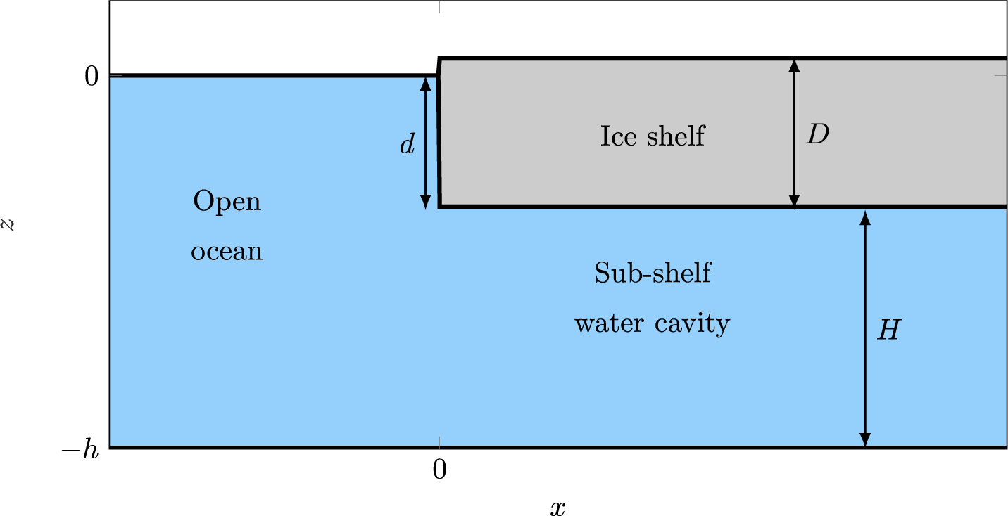
Schematic (not to scale) of the equilibrium geometry.

A floating ice shelf of uniform thickness, D, occupies the water surface for $x>0$
. It has an Archimedean draught, such that its lower surface is at
$x>0$
. It has an Archimedean draught, such that its lower surface is at $z=-d$
in equilibrium, where
$z=-d$
in equilibrium, where
 $$ \begin{align*} d = \frac{\rho_{\text{i}}\,D}{\rho_{\text{w}}}, \end{align*} $$
in which $\rho _{\text {i}}=922.5$
kg m
$\rho _{\text {i}}=922.5$
kg m $^{-3}$
and
$^{-3}$
and $\rho _{\text {w}}=1025$
kg m
$\rho _{\text {w}}=1025$
kg m $^{-3}$
are the ice and water densities, respectively (where the ice-shelf density is, for example, approximately at the top end of the values given for the Amery Ice Shelf by [Reference Fricker, Popov, Allison and Young17]), so that
$^{-3}$
are the ice and water densities, respectively (where the ice-shelf density is, for example, approximately at the top end of the values given for the Amery Ice Shelf by [Reference Fricker, Popov, Allison and Young17]), so that $\rho _{\text {i}}/\rho _{\text {w}}=0.9$
. Therefore, the ice shelf encloses a water cavity of equilibrium depth
$\rho _{\text {i}}/\rho _{\text {w}}=0.9$
. Therefore, the ice shelf encloses a water cavity of equilibrium depth $H\equiv {}h-d$
(Figure 1). The water domain for
$H\equiv {}h-d$
(Figure 1). The water domain for $x<0$
is referred to as the open ocean.
$x<0$
is referred to as the open ocean.
Water motion is modelled using linear potential-flow theory, assuming that the water is inviscid and incompressible, the motion is irrotational, and amplitudes are much smaller than the wavelengths involved. The water displacement field (rather the the velocity field) is defined as the gradient of a scalar potential, $\Phi (x,z,t)$
, where t denotes time. The displacement potential satisfies Laplace’s equation,
$\Phi (x,z,t)$
, where t denotes time. The displacement potential satisfies Laplace’s equation,
 $$ \begin{align*} \boldsymbol{\nabla}^2\,\Phi = 0, \end{align*} $$
throughout the linearized water domain (open water and sub-shelf water cavity), plus a no-normal flow condition on the seabed, such that
 $$ \begin{align*} \Phi_{z} = 0 \quad\text{for } x\in\mathbb{R} \text{ and } z=-h. \end{align*} $$
The ice shelf is modelled as an elastic solid, with horizontal and vertical displacements, $U(x,z,t)$
and
$U(x,z,t)$
and $W(x,z,t)$
, respectively. The displacements satisfy the equations of linear elasticity,
$W(x,z,t)$
, respectively. The displacements satisfy the equations of linear elasticity,
 $$ \begin{align} \rho_{\text{i}}\,U_{tt} =\sigma_{11,x} + \sigma_{12,z} \quad\text{and}\quad \rho_{\text{i}}\,W_{tt} = \sigma_{12,x} + \sigma_{22,z}-\rho_{\text{i}}\,g \end{align} $$
for $x>0$
and
$x>0$
and $-d<z<D-d$
. In (2.1),
$-d<z<D-d$
. In (2.1), $g=9.81$
m s
$g=9.81$
m s $^{-2}$
is gravitational acceleration and
$^{-2}$
is gravitational acceleration and $\sigma _{ij}$
(
$\sigma _{ij}$
( $i,j=1,2$
) are the components of the Cauchy stress tensor. The ice-shelf motion is coupled to the water motion via kinematic and dynamic conditions along its lower surface (
$i,j=1,2$
) are the components of the Cauchy stress tensor. The ice-shelf motion is coupled to the water motion via kinematic and dynamic conditions along its lower surface ( $x>0$
and
$x>0$
and $z=-d$
), and along the submerged portion of the shelf front (
$z=-d$
), and along the submerged portion of the shelf front ( $x=0$
and
$x=0$
and $-d<z<0$
) [Reference Bennetts, Williams and Porter10]. Standard conditions are satisfied along its boundaries in contact with the atmosphere [Reference Bennetts, Williams and Porter10].
$-d<z<0$
) [Reference Bennetts, Williams and Porter10]. Standard conditions are satisfied along its boundaries in contact with the atmosphere [Reference Bennetts, Williams and Porter10].
Motions are excited by a rightwards propagating incident wave packet from the open ocean. Following [Reference Bennetts and Meylan9], the incident packet is defined via the free surface elevation in the open ocean, $\eta (x,t) = \Phi _{z}(x,0{,t})$
(
$\eta (x,t) = \Phi _{z}(x,0{,t})$
( $x<0$
), such that the incident packet creates the surface elevation
$x<0$
), such that the incident packet creates the surface elevation
 $$ \begin{align}{} \eta(x,t)=\eta_{\text{inc}}(x,t)\equiv\textrm{Re}\bigg\{\!\int_0^{\infty} {A}(k)\,\varphi_{\text{inc}}(x)\,{e}^{-{i}\omega t} \,{d} k\bigg\}, \end{align} $$
where $\varphi _{\text {inc}}={e}^{{i}kx}$
and
$\varphi _{\text {inc}}={e}^{{i}kx}$
and ${A}$
is the Gaussian
${A}$
is the Gaussian
 $$ \begin{align} {A}(k) = A_0\,{e}^{-(k-k_{\text{c}})^2/(2\,\sigma^2)-{i}kx_{\text{c}}}{,} \end{align} $$
which is chosen for convenience rather than based on observations. Here, $A_{0}$
is the packet amplitude (in wavenumber space),
$A_{0}$
is the packet amplitude (in wavenumber space), $k_{\text {c}}$
is its central wavenumber,
$k_{\text {c}}$
is its central wavenumber, $\sigma $
is its width (that is, standard deviation) and
$\sigma $
is its width (that is, standard deviation) and $x_{\text {c}}$
is the physical location of the packet centre at
$x_{\text {c}}$
is the physical location of the packet centre at $t=0$
. For the results presented in Section 4, the incident packet is separated from the ice shelf at
$t=0$
. For the results presented in Section 4, the incident packet is separated from the ice shelf at $t=0$
by setting
$t=0$
by setting $x_{\text {c}}=-3/\sigma $
. Note that (2.2) sets the wavenumber k as the spectral parameter for the problem, such that the angular frequency,
$x_{\text {c}}=-3/\sigma $
. Note that (2.2) sets the wavenumber k as the spectral parameter for the problem, such that the angular frequency, $\omega $
, is treated as a function of k, via the standard open water dispersion relation (3.2a).
$\omega $
, is treated as a function of k, via the standard open water dispersion relation (3.2a).
In the absence of an ice shelf, the incident wave packet energy across the spatial domain, $\mathcal {E}(t)$
, does not change as the packet propagates and, hence,
$\mathcal {E}(t)$
, does not change as the packet propagates and, hence, $\mathcal {E}(t)=\mathcal {E}(0)\equiv \mathcal {E}_{0}$
. Noting that the energy at
$\mathcal {E}(t)=\mathcal {E}(0)\equiv \mathcal {E}_{0}$
. Noting that the energy at $t=0$
is proportional to
$t=0$
is proportional to $|\eta (x,0)|^2$
[Reference Jeschke and Wojtan24] and that
$|\eta (x,0)|^2$
[Reference Jeschke and Wojtan24] and that ${A}(k)$
is the Fourier transform of the initial wave profile,
${A}(k)$
is the Fourier transform of the initial wave profile, $\eta (x,0)$
, Parseval’s theorem implies
$\eta (x,0)$
, Parseval’s theorem implies
 $$ \begin{align} \mathcal{E}_{0}\propto \int_{-\infty}^{\infty} |\eta(x,0)|^2\,{d}x = \int_{0}^{\infty} |{A}(k)|^2\,{d}k. \end{align} $$
Substituting (2.3) into (2.4),
 $$ \begin{align*} \mathcal{E}_{0} &\propto \int_{0}^{\infty} |A_0\,{ e}^{-(k-k_c)^2/(2\,\sigma^2)}|^2\,{d}k \\ &= A_0^2\,\int_{0}^{\infty} \,{e}^{-(k-k_c)^2/\sigma^2}\,{d}k \\ &\approx A_0^2\,\sigma\sqrt{\pi}, \end{align*} $$
where the final result follows from the assumption that $k_{c}\gg \sigma $
. Thus, different wave packets have the same energy,
$k_{c}\gg \sigma $
. Thus, different wave packets have the same energy, $\mathcal {E}_{0}$
, if they share the same value of
$\mathcal {E}_{0}$
, if they share the same value of $A_{0}^{2}\,\sigma $
.
$A_{0}^{2}\,\sigma $
.
3 Approximate solution
Following [Reference Bennetts, Williams and Porter10], a thin-plate (depth-averaged) approximation is applied to the ice-shelf motions based on the plane stress and plane strain assumptions. The thin-plate approximation uses the ansatzes
 $$ \begin{align*} U(x,z,t) = \mathcal{U}(x,t) - (z+d-D/2) \mathcal{W}_{x}(x,t)\quad \text{and}\quad W(x,z,t) = \mathcal{W}(x,t), \end{align*} $$
where $\mathcal {U}$
and
$\mathcal {U}$
and $\mathcal {W}$
represent the extensional and flexural motions, respectively.
$\mathcal {W}$
represent the extensional and flexural motions, respectively.
The thin-plate approximation is combined with a single-mode (depth-averaged) approximation for the water motion [Reference Bennetts, Biggs and Porter7], which assumes the vertical profile through the water column is that of the propagating wave mode. Thus, separate ansatzes are applied to the potential in the open ocean and sub-shelf water cavity regions, such that
 $$ \begin{align} \Phi(x,z,t) = \frac{g}{\omega^2}\,\varphi(x)\frac{\cosh \{k\,(z+h)\}}{\cosh{k\,h}}\,{ e}^{-{i}\omega t} & \quad\text{for } x<0 \end{align} $$
 $$ \begin{align} \text{and}\quad \Phi(x,z,t) = \frac{g}{\omega^2}\,\psi(x) \frac{\cosh \{\kappa\,(z+h)\}}{\cosh{\kappa\,H}}\,{e}^{-{i}\omega t} & \quad\text{for } x>0. \end{align} $$
The wavenumbers k and $\kappa $
satisfy the dispersion relations
$\kappa $
satisfy the dispersion relations
 $$ \begin{align} k\,\tanh(k\,h) & = \frac{\omega^{2}}{g}\quad\text{and} \end{align} $$
 $$ \begin{align} \{F\,\kappa^{4} - J\,\omega^{2}\,\kappa^{2} + 1 -m\,\omega^{2}\}\,\kappa\,\tanh(\kappa\,H) & = \frac{\omega^{2}}{g}, \end{align} $$
where F, J and m are scaled versions of the ice shelf flexural rigidity, rotational inertia and mass, respectively. They are defined as
 $$ \begin{align*} F = \frac{E\,D^{3}}{12\,(1-\nu^{2})\,\rho_{\text{w}}\,g}, \quad J = \frac{\rho_{\text{i}}\,D^{3}}{12\,\rho_{w}\,g} \quad\text{and}\quad m = \frac{\rho_{\text{i}}\,D}{\rho_{w}\,g}{,} \end{align*} $$
where $E=10$
GPa and
$E=10$
GPa and $\nu =0.3$
are the Young’s modulus and Poisson’s ratio of the ice shelf [Reference Liang, Pitt and Bennetts28]. The single-mode approximation (3.1a) maps the problem to the frequency domain through the assumption that the water motions are at a prescribed angular frequency,
$\nu =0.3$
are the Young’s modulus and Poisson’s ratio of the ice shelf [Reference Liang, Pitt and Bennetts28]. The single-mode approximation (3.1a) maps the problem to the frequency domain through the assumption that the water motions are at a prescribed angular frequency, $\omega $
. A compatible mapping is applied to the ice-shelf motions such that
$\omega $
. A compatible mapping is applied to the ice-shelf motions such that
 $$ \begin{align*} \mathcal{U}(x,t)=u(x)\,{e}^{-{i}\omega t} \quad\text{and}\quad \mathcal{W}(x,t)=w(x)\,{e}^{-{i}\omega t}. \end{align*} $$
The unknowns in the frequency domain are complex-valued functions, that is, $\varphi $
,
$\varphi $
, $\psi $
, u,
$\psi $
, u, $w\in \mathbb {C}$
.
$w\in \mathbb {C}$
.
The governing equations of the thin-plate/single-mode approximation are
 $$ \begin{align} \varphi"+k^{2}\,\varphi & = 0 \quad\text{for } x<0, \end{align} $$
 $$ \begin{align} a\,\psi" + b\,\psi + \frac{\omega^{2}}{g}\,w & = 0 \quad\text{for } x>0, \end{align} $$
 $$ \begin{align} F\,w"" + J\,\omega^{2}\,w" + (1-m\,\omega^{2})\,w - \psi & = 0 \quad\text{for } x>0\quad\text{and} \end{align} $$
 $$ \begin{align} G\,u" + m\,\omega^{2}\,u & = 0 \quad\text{for } x>0, \end{align} $$
where
 $$ \begin{align*} a = \int_{-h}^{-d}\frac{\cosh{^{2}} \{\kappa\,(z+h)\}}{\cosh{^{2}}(\kappa\,H)} \,{d}z, \quad b = \kappa^{2}\,a -\kappa\,\tanh(\kappa\,H) \end{align*} $$
and $G=E\,D/\{\rho _{\text {w}}\,g\,(1-\nu ^{2})\}$
. The solutions are subject to the jump conditions
$G=E\,D/\{\rho _{\text {w}}\,g\,(1-\nu ^{2})\}$
. The solutions are subject to the jump conditions
 $$ \begin{align} a_{0}\,\varphi = a\,\psi \quad\text{and}\quad a_{1}\,\varphi' = a_{0}\,\psi' + \frac{\omega^{2}}{g}\,\{v_{0}\,u - v_{1}\,w'\} \quad\text{for } x=0, \end{align} $$
and the shelf front conditions
 $$ \begin{align} F\,w" + v_{1}\,\varphi = 0 ,\quad F\,w"' + J\,\omega^{2}\,w' = 0 \quad\text{and}\quad G\,u' + v_{0}\,\varphi = 0 \end{align} $$
for $x=0$
, where
$x=0$
, where
 $$ \begin{align*} a_{0} & = \int_{-h}^{0}\frac{\cosh{^{2}} \{k\,(z+h)\}}{\cosh{^{2}}(k\,h)} \,{d}z,\\ a_{1} & = \int_{-h}^{-d}\,\frac{\cosh \{k\,(z+h)\}\,\cosh\{\kappa(z+h)\}}{\cosh(k\,h)\,\cosh(\kappa H)} \,{d}z,\\ v_{0} & = \int_{-d}^{0}\,\frac{\cosh \{k\,(z+h)\}}{\cosh(k\,h)} \,{d}z\quad \text{and}\\ v_{1} & = \int_{-d}^{0}\,\frac{\cosh \{k\,(z+h)\}}{\cosh(k\,h)} (z+d-D/2)\,{d}z. \end{align*} $$
The second-order ordinary differential equation (ODE) in the open water region (3.3a) can be solved up to unknown constants. It is expressed as
 $$ \begin{align*} \varphi(x) = \varphi_{\text{inc}}(x) + R\,{e}^{-{i}kx}, \end{align*} $$
where the second term on the right-hand side is the wave reflected by the ice shelf, which has amplitude $R\in \mathbb {C}$
. The system of ODEs in the ice shelf/water cavity region ((3.3b)–(3.3d)) can also be solved to give
$R\in \mathbb {C}$
. The system of ODEs in the ice shelf/water cavity region ((3.3b)–(3.3d)) can also be solved to give
 $$ \begin{align*} \psi(x) & = T_{\text{cav}} {e}^{{i}\kappa x} + \sum_{j={1,2}} T_{\text{cav}}^{(-j)}\,{e}^{{i} \kappa_{-j}x},\\ w(x) &= T_{\text{flex}} {e}^{{i}\kappa x} + \sum_{j={1,2}} T_{\text{flex}}^{(-j)}\,{e}^{{i} \kappa_{-j}x}\quad \text{and}\quad\\ u(x) &= T_{\text{ext}}\,{e}^{{i}qx}. \end{align*} $$
The wavenumbers $\kappa _{-j}\in \mathbb {R}+{i}\,\mathbb {R}_{+}$
(
$\kappa _{-j}\in \mathbb {R}+{i}\,\mathbb {R}_{+}$
( $j=1,2$
) are the roots of the quartic equation (Appendix A),
$j=1,2$
) are the roots of the quartic equation (Appendix A),
 $$ \begin{align} a\,(F\,\kappa_{-j}^{4}-J\,\omega^{2}\,\kappa_{-j}^{2}+1-m\,\omega^{2}) + \{F\,(\kappa^{2}+\kappa_{-j}^{2})-J\,\omega^{2}\}\,\kappa\,\tanh(\kappa\,H)=0, \end{align} $$
which approximate complex-valued roots of (3.2b) and are typically such that ${\kappa _{-2}=-\overline {\kappa _{-1}}}$
. The extensional wavenumber,
${\kappa _{-2}=-\overline {\kappa _{-1}}}$
. The extensional wavenumber, $q\in \mathbb {R}_{+}$
, is
$q\in \mathbb {R}_{+}$
, is
 $$ \begin{align*} q = \omega\,\sqrt{\frac{\rho_{\text{i}}\,(1-\nu^2)}{E}}. \end{align*} $$
The amplitude of the transmitted propagating wave in the cavity is related to the flexural wave in the shelf by (Appendix A),
 $$ \begin{align} T_{\text{cav}}=\frac{\omega^{2}}{{g\,}\kappa\,\tanh(\kappa\,H)}\,T_{\text{flex}}, \end{align} $$
and similarly,
 $$ \begin{align} T_{\text{cav}}^{(-j)}= \frac{{-\{}F\,(\kappa^{2}+\kappa_{-j}^{2})-J\,\omega^{2}{\}\,\kappa\,\tanh(\kappa\,H)}}{a}\,T_{\text{flex}}^{(-j)} \quad\text{for } j=1,2. \end{align} $$
The jump conditions (3.4) and shelf-front conditions (3.5) are applied to calculate the five unknown amplitudes, R, $T_{\text {flex}}$
,
$T_{\text {flex}}$
, $T_{\text {flex}}^{(-j)}$
(
$T_{\text {flex}}^{(-j)}$
( $j=1,2$
) and
$j=1,2$
) and $T_{\text {ext}}$
, thus completing the frequency-domain solution.
$T_{\text {ext}}$
, thus completing the frequency-domain solution.
The scaling used in the single-mode approximation (3.1a) is such that the incident free surface displacement is identical to the incident potential, $\varphi _{\text {inc}}$
. Therefore, the time-domain solution is obtained as a superposition of frequency-domain solutions, such that, for example,
$\varphi _{\text {inc}}$
. Therefore, the time-domain solution is obtained as a superposition of frequency-domain solutions, such that, for example,
 $$ \begin{align*} \eta(x,t)=\textrm{Re}\bigg\{\!\int_0^{\infty} {A}(k)\,\varphi(x)\,{e}^{-{i}\omega t} \, {d} k\bigg\}{\quad\text{for } x<0.} \end{align*} $$
The only non-zero component of the strain tensor is [Reference Bennetts, Williams and Porter10]
 $$ \begin{align} \epsilon(x,z,t)=\textrm{Re}\bigg\{\!\int_0^{\infty} {A}(k)\varepsilon(x,z)\,{e}^{-{i}\omega t} \,{d} k\bigg\} \quad\text{where } \varepsilon(x,z)= u'-(z+d-D/2)w" \end{align} $$
for $x>0$
and
$x>0$
and $-d<z<D-d$
. It can be decomposed as
$-d<z<D-d$
. It can be decomposed as $\epsilon = \epsilon _{\text {flex}}+\epsilon _{\text {ext}}$
, where
$\epsilon = \epsilon _{\text {flex}}+\epsilon _{\text {ext}}$
, where $\epsilon _{\text {flex}}$
and
$\epsilon _{\text {flex}}$
and $ \epsilon _{\text {ext}}$
are the strains produced by the flexural and extensional waves, respectively. They are
$ \epsilon _{\text {ext}}$
are the strains produced by the flexural and extensional waves, respectively. They are
 $$ \begin{align} \begin{aligned} \epsilon_{\text{flex}}(x,z,t)&=\textrm{Re}\bigg\{\!\int_0^{\infty} {A}(k)\,\varepsilon_{\text{flex}}(x,z)\,{e}^{-{i}\omega t}\,{d} k\bigg\}\quad \text{and} \\ \epsilon_{\text{ext}}(x,t)&=\textrm{Re}\bigg\{\!\int_0^{\infty} {A}(k) \varepsilon_{\text{ext}}(x)\,{e}^{-{i}\omega t}\,{d} k\bigg\}, \end{aligned} \end{align} $$
in which
 $$ \begin{align} \varepsilon_{\text{flex}}(x,z)=-(z+d-D/2)\,w" \quad\text{and}\quad \varepsilon_{\text{ext}}(x) =u'. \end{align} $$
4 Results
4.1 Frequency-domain analysis
Figure 2(a) shows the ratio of the maximum strain caused by extensional waves to the maximum strain caused by flexural waves in the frequency domain, that is, $\max \vert \varepsilon _{\text {ext}}\vert /\!\max \vert \varepsilon _{\text {flex}}\vert $
(3.11), as a function of ice-shelf thickness,
$\max \vert \varepsilon _{\text {ext}}\vert /\!\max \vert \varepsilon _{\text {flex}}\vert $
(3.11), as a function of ice-shelf thickness, $D\in [100\text {\,m},500\text {\,m}]$
, and wave period,
$D\in [100\text {\,m},500\text {\,m}]$
, and wave period, $T\in [10\text {\,s},30\text {\,s}]$
, where
$T\in [10\text {\,s},30\text {\,s}]$
, where $T=2\,\pi /\omega $
, that is, the swell regime. The water cavity depth is fixed at
$T=2\,\pi /\omega $
, that is, the swell regime. The water cavity depth is fixed at $H=800$
m. The maximum values are calculated over the ice-shelf domain,
$H=800$
m. The maximum values are calculated over the ice-shelf domain, $x>0$
and
$x>0$
and $-d<z<D-d$
, noting that the extensional motions depend only on horizontal location, x, and the magnitudes of the flexural motions are symmetric about the ice-shelf mid-plane,
$-d<z<D-d$
, noting that the extensional motions depend only on horizontal location, x, and the magnitudes of the flexural motions are symmetric about the ice-shelf mid-plane, $z=D/2-d$
, and attain maximum values at the upper/lower surfaces,
$z=D/2-d$
, and attain maximum values at the upper/lower surfaces, $z=-d$
and
$z=-d$
and $D-d$
. There is a (yellow) band of width 2–4 s where the ratio is greatest (
$D-d$
. There is a (yellow) band of width 2–4 s where the ratio is greatest ( ${\max \vert \varepsilon _{\text {ext}}\vert /\!\max \vert \varepsilon _{\text {flex}}\vert }\approx {}1$
), that is, the maximum strains due to extensional and flexural waves are almost identical. The band moves from being centred at
${\max \vert \varepsilon _{\text {ext}}\vert /\!\max \vert \varepsilon _{\text {flex}}\vert }\approx {}1$
), that is, the maximum strains due to extensional and flexural waves are almost identical. The band moves from being centred at $T\approx {}10$
s for
$T\approx {}10$
s for $D=100$
m to
$D=100$
m to $T\approx {}20$
s for
$T\approx {}20$
s for $D=500$
m. On the shorter wave period side of the band, the ratio decreases slightly to no less than
$D=500$
m. On the shorter wave period side of the band, the ratio decreases slightly to no less than ${\max \vert \varepsilon _{\text {ext}}\vert /\!\max \vert \varepsilon _{\text {flex}}\vert =}0.5$
, indicating that strains due to extensional waves remain comparable to those due to flexural waves. On the longer wave period side of the band, the ratio decreases sharply to
${\max \vert \varepsilon _{\text {ext}}\vert /\!\max \vert \varepsilon _{\text {flex}}\vert =}0.5$
, indicating that strains due to extensional waves remain comparable to those due to flexural waves. On the longer wave period side of the band, the ratio decreases sharply to ${\max \vert \varepsilon _{\text {ext}}\vert /\!\max \vert \varepsilon _{\text {flex}}\vert }\approx {}0$
(on the linear scale shown), indicating strains due to flexural waves are dominant.
${\max \vert \varepsilon _{\text {ext}}\vert /\!\max \vert \varepsilon _{\text {flex}}\vert }\approx {}0$
(on the linear scale shown), indicating strains due to flexural waves are dominant.
Heatmaps showing ratios of (a) maximum strain due to extensional waves to maximum strain due to flexural waves in the frequency domain, $\max \vert \varepsilon _{\text {ext}}\vert /\!\max \vert \varepsilon _{\text {flex}}\vert $
, and (b) phase speed of the extensional wave to that of the flexural wave,
$\max \vert \varepsilon _{\text {ext}}\vert /\!\max \vert \varepsilon _{\text {flex}}\vert $
, and (b) phase speed of the extensional wave to that of the flexural wave, $c_{\text {ext}}/c_{\text {flex}}$
, versus wave period, T, and ice-shelf thickness, D.
$c_{\text {ext}}/c_{\text {flex}}$
, versus wave period, T, and ice-shelf thickness, D.

Figure 2(b) shows the corresponding ratio of the phase speeds of the extensional and flexural waves respectively
 $$ \begin{align*} c_{\text{ext}} = \frac{\omega}{q} \quad\text{and}\quad c_{\text{flex}} = \frac{\omega}{\kappa}. \end{align*} $$
The ratio is greater than ten ( $c_{\text {ext}}/c_{\text {flex}}>10$
) over the considered wave period and ice thickness region, which indicates the extensional waves are at least an order of magnitude faster than the flexural waves. The ratio is
$c_{\text {ext}}/c_{\text {flex}}>10$
) over the considered wave period and ice thickness region, which indicates the extensional waves are at least an order of magnitude faster than the flexural waves. The ratio is ${c_{\text {ext}}/c_{\text {flex}}}\approx {}10$
–15 in the wave period–ice thickness region where the strains due to extensional and flexural motions are comparable (
${c_{\text {ext}}/c_{\text {flex}}}\approx {}10$
–15 in the wave period–ice thickness region where the strains due to extensional and flexural motions are comparable ( $\max \vert \varepsilon _{\text {ext}}\vert /\!\max \vert \varepsilon _{\text {flex}}\vert \approx {}1$
). The ratio reaches up to
$\max \vert \varepsilon _{\text {ext}}\vert /\!\max \vert \varepsilon _{\text {flex}}\vert \approx {}1$
). The ratio reaches up to ${c_{\text {ext}}/c_{\text {flex}}}\approx {}25$
for the longest wave periods and thinnest ice considered, which is the regime in which flexural motions dominate strain (
${c_{\text {ext}}/c_{\text {flex}}}\approx {}25$
for the longest wave periods and thinnest ice considered, which is the regime in which flexural motions dominate strain ( $\max \vert \varepsilon _{\text {ext}}\vert /\!\max \vert \varepsilon _{\text {flex}}\vert \approx {}0$
).
$\max \vert \varepsilon _{\text {ext}}\vert /\!\max \vert \varepsilon _{\text {flex}}\vert \approx {}0$
).
4.2 Time domain: case study
Consider a Gaussian incident wave packet (2.2) interacting with a $D=200$
m-thick ice shelf. The packet has peak wave period
$D=200$
m-thick ice shelf. The packet has peak wave period ${T_{\text {peak}}=15}$
s, where
${T_{\text {peak}}=15}$
s, where $T_{\text {peak}}=2\,\pi /\omega _{\text {peak}}$
and
$T_{\text {peak}}=2\,\pi /\omega _{\text {peak}}$
and $\omega _{\text {peak}}= \sqrt {g\,k_{\text {c}}\,\tanh (k_{\text {c}}\,h)}$
, such that the peak of the packet is where the strains due to extensional and flexural waves are of almost identical magnitude. The packet width is
$\omega _{\text {peak}}= \sqrt {g\,k_{\text {c}}\,\tanh (k_{\text {c}}\,h)}$
, such that the peak of the packet is where the strains due to extensional and flexural waves are of almost identical magnitude. The packet width is $\sigma =2\times 10^{-3}$
m
$\sigma =2\times 10^{-3}$
m $^{-1}$
, which corresponds to a width of
$^{-1}$
, which corresponds to a width of $\approx {}15$
s in wave period, which is skewed towards longer periods around
$\approx {}15$
s in wave period, which is skewed towards longer periods around $T_{\text {peak}}$
, that is,
$T_{\text {peak}}$
, that is, $T_{\text {peak}}$
is not at the centre of the packet in terms of wave periods.
$T_{\text {peak}}$
is not at the centre of the packet in terms of wave periods.
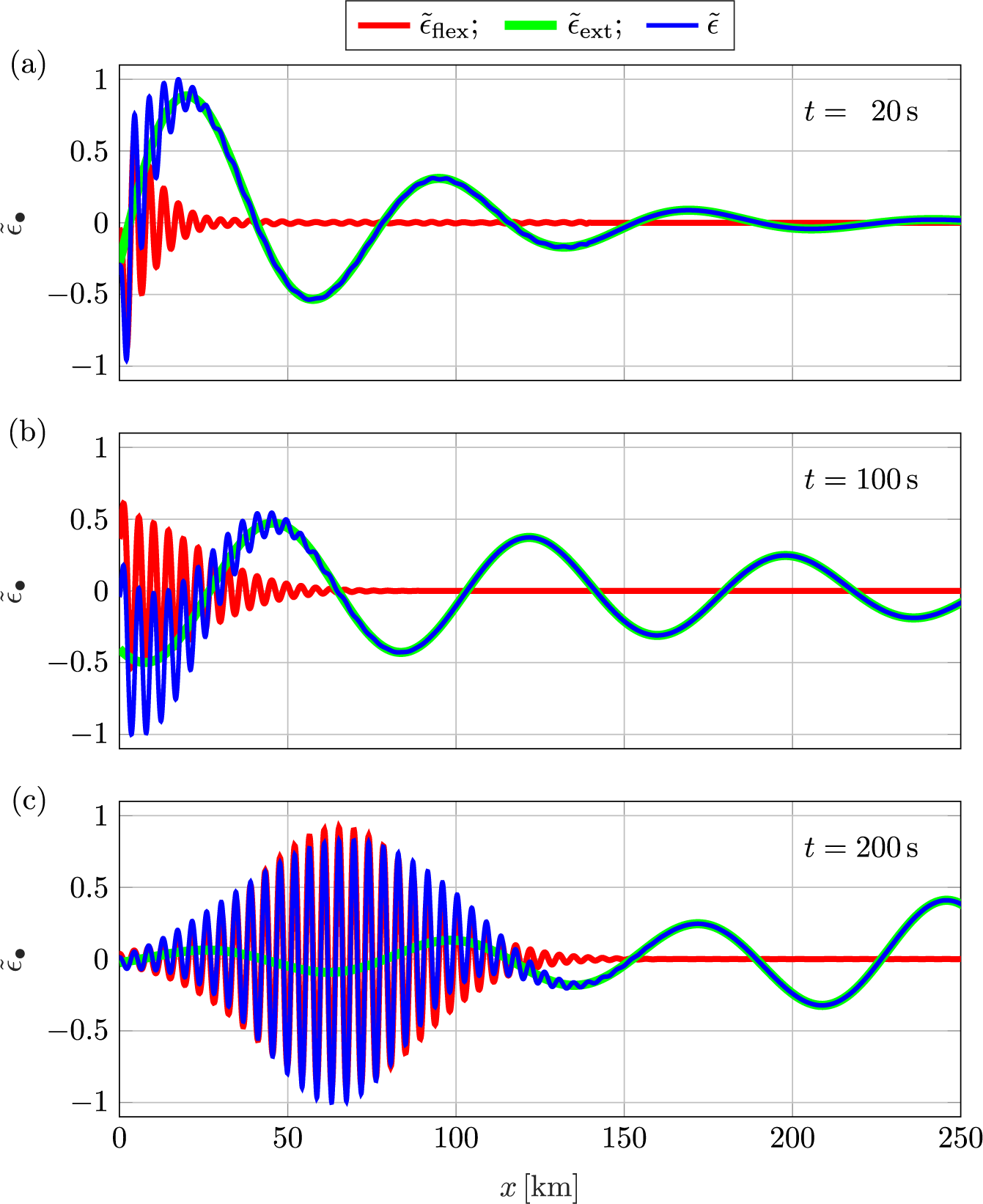
When the leading edge of the incident wave packet interacts with the shelf front at $t=20$
s (Figure 3a), it generates (i) extensional strain waves in the ice shelf,
$t=20$
s (Figure 3a), it generates (i) extensional strain waves in the ice shelf, $\epsilon _{\text {ext}}$
, which are identified by the vertical bands that alternate between positive and negative strain, and propagate quickly along the shelf, such that they can be detected
$\epsilon _{\text {ext}}$
, which are identified by the vertical bands that alternate between positive and negative strain, and propagate quickly along the shelf, such that they can be detected $>200$
km from the shelf front, and (ii) flexural strain waves,
$>200$
km from the shelf front, and (ii) flexural strain waves, $\epsilon _{\text {flex}}$
, which are coupled to motions in the sub-shelf water cavity and are confined to
$\epsilon _{\text {flex}}$
, which are coupled to motions in the sub-shelf water cavity and are confined to $\approx {}30$
km from the shelf front. When the peak of the packet reaches the shelf front at
$\approx {}30$
km from the shelf front. When the peak of the packet reaches the shelf front at $t=100$
s (Figure 3b), there is an interval of
$t=100$
s (Figure 3b), there is an interval of $\approx {}70$
km from the shelf front where flexural and extensional waves co-exist, and with only extensional waves farther from the shelf front. When the entire packet has interacted with the shelf at
$\approx {}70$
km from the shelf front where flexural and extensional waves co-exist, and with only extensional waves farther from the shelf front. When the entire packet has interacted with the shelf at $t=200$
s (Figure 3c), the extensional and flexural waves in the ice shelf have separated, due to the large difference in their celerities, with the flexural waves occupying up to
$t=200$
s (Figure 3c), the extensional and flexural waves in the ice shelf have separated, due to the large difference in their celerities, with the flexural waves occupying up to $x\approx {}125$
km and identified by the antisymmetric strains about the mid-plane of the shelf.
$x\approx {}125$
km and identified by the antisymmetric strains about the mid-plane of the shelf.
Snapshots of the strain field, $\epsilon (x,z,t)$
(3.9), in a
$\epsilon (x,z,t)$
(3.9), in a $D=200$
m-thick ice shelf, forced by a Gaussian incident wave packet (2.2) with a peak period
$D=200$
m-thick ice shelf, forced by a Gaussian incident wave packet (2.2) with a peak period $T_{\text {peak}} = 15$
s and width
$T_{\text {peak}} = 15$
s and width $\sigma = 2 \times 10^{-3}$
m
$\sigma = 2 \times 10^{-3}$
m $^{-1}$
. The free surface elevation of the incident packet,
$^{-1}$
. The free surface elevation of the incident packet, $\eta {(x,t)}=\eta _{\text {inc}}{(x,t)}$
, is shown in the open ocean (black curve) and the displacement potential is shown in the sub-shelf water cavity,
$\eta {(x,t)}=\eta _{\text {inc}}{(x,t)}$
, is shown in the open ocean (black curve) and the displacement potential is shown in the sub-shelf water cavity, $\Phi (x,z,t)$
(3.1b) (scaled by a factor
$\Phi (x,z,t)$
(3.1b) (scaled by a factor $10^{-3}$
to match the colour bar for strain). The snapshots are at times (a)
$10^{-3}$
to match the colour bar for strain). The snapshots are at times (a) $t = 20$
s, (b)
$t = 20$
s, (b) $100$
s and (c)
$100$
s and (c) $200$
s.
$200$
s.

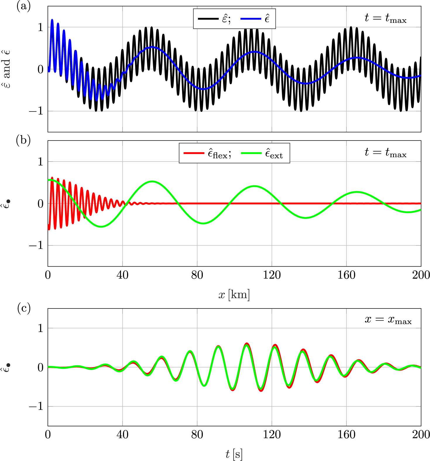
The strain, $\epsilon $
, generally attains its maximum values along either its upper surface (
$\epsilon $
, generally attains its maximum values along either its upper surface ( $z=D-d$
) or its lower surface (
$z=D-d$
) or its lower surface ( $z=-d$
). Taking the lower surface for the purpose of illustration and using the normalized strains
$z=-d$
). Taking the lower surface for the purpose of illustration and using the normalized strains
 $$ \begin{align} {\tilde{\epsilon}(x,t)} & = \epsilon(x,{z=-d},t)/\!\max_{x}|\epsilon(x,{z=-d},t)|, \end{align} $$
 $$ \begin{align} {\tilde{\epsilon}_{\text{flex}}(x,t)} & = \epsilon_{\text{flex}}(x,{z=-d},t) /\!\max_{x}|\epsilon(x,{z=-d},t)| \quad\text{and} \end{align} $$
 $$ \begin{align} { \tilde{\epsilon}_{\text{ext}}(x,t)} & = \epsilon_{\text{ext}}(x,t)/\!\max_{x}|\epsilon(x,{z=-d},t)|, \end{align} $$
there is a transition in the strain profile being dominated by the extensional waves during the early phase of the wave packet–ice shelf interaction (panel a), to an increasing contribution from the flexural waves (panel b), to flexural waves dominating the strain over the first 100 km (panel c) (as expected from Figure 4). In all cases, the strain magnitudes reach their maximum values ( $\vert {\tilde {\epsilon }}\vert =1$
) at locations where there are coherent interactions between the extensional and flexural waves.
$\vert {\tilde {\epsilon }}\vert =1$
) at locations where there are coherent interactions between the extensional and flexural waves.
Snapshots of the strain profile along the bottom of the ice shelf (normalized by its maximum value at that instant of time; (4.1a)), $\tilde {\epsilon }(x,t)$
(blue curves) for the case shown in Figure 3. The corresponding contributions to the strain due to flexural waves,
$\tilde {\epsilon }(x,t)$
(blue curves) for the case shown in Figure 3. The corresponding contributions to the strain due to flexural waves, $\tilde {\epsilon }_{\text {flex}}(x,t)$
(red), and extensional waves,
$\tilde {\epsilon }_{\text {flex}}(x,t)$
(red), and extensional waves, $\tilde {\epsilon }_{\text {ext}}(x,t)$
(green), are superimposed.
$\tilde {\epsilon }_{\text {ext}}(x,t)$
(green), are superimposed.

The time when the maximum strain magnitude is attained is
 $$ \begin{align} t_{\max}=\mathrm{arg\max}\Big\{\max_{x}\vert\epsilon(x,z=-d,t)\vert\Big\}. \end{align} $$
The strain profile at $t=t_{\max }\approx {}109$
s is similar to the strain profile in the frequency domain at the peak period
$t=t_{\max }\approx {}109$
s is similar to the strain profile in the frequency domain at the peak period $T_{\text {peak}}$
/central wavenumber
$T_{\text {peak}}$
/central wavenumber $k_{\text {c}}$
and corresponding amplitude,
$k_{\text {c}}$
and corresponding amplitude, $A_{0}\equiv {A}(k_{\text {c}})$
, as illustrated by similarity of the profiles
$A_{0}\equiv {A}(k_{\text {c}})$
, as illustrated by similarity of the profiles
 $$ \begin{align} {\hat{\varepsilon}(x)} & { =\textrm{Re}\{\varepsilon(x,{z=-d}:k_{\text{c}})\}}\quad\text{and} \end{align} $$
 $$ \begin{align} { \hat{\epsilon}(x,t)} & = \epsilon(x,{z=-d},t)/\!\max_{x}|{A}_{0}\,\varepsilon(x,{z=-d}:\omega(k_{\text{c}}))| \end{align} $$
(a) The strain profile relative to the maximum strain in the corresponding frequency-domain problem, $\hat {\epsilon }(x,t)$
(4.3b), at the time when the maximum strain magnitude is attained,
$\hat {\epsilon }(x,t)$
(4.3b), at the time when the maximum strain magnitude is attained, $t=t_{\max }$
(4.2) (blue curve), superimposed on the frequency-domain strain profile,
$t=t_{\max }$
(4.2) (blue curve), superimposed on the frequency-domain strain profile, $\hat {\varepsilon }(x)$
((4.3a); black). (b) Corresponding strain profiles due to flexural waves,
$\hat {\varepsilon }(x)$
((4.3a); black). (b) Corresponding strain profiles due to flexural waves, $\hat {\epsilon }_{\text {flex}}(x,t)$
((4.4a); red), and extensional waves,
$\hat {\epsilon }_{\text {flex}}(x,t)$
((4.4a); red), and extensional waves, $\hat {\epsilon }_{\text {ext}}(x,t)$
((4.4b); green). (c) Time series of the strains due to flexural and extensional waves at the location where the maximum strain magnitude is attained,
$\hat {\epsilon }_{\text {ext}}(x,t)$
((4.4b); green). (c) Time series of the strains due to flexural and extensional waves at the location where the maximum strain magnitude is attained, $x=x_{\max }$
(4.5).
$x=x_{\max }$
(4.5).

at $t=t_{\max }$
(Figure 5a). The main difference is that the short-wave component of the strain in the time domain exists only up to 30–40 km from the shelf front. Over this interval, the amplitudes of the strain due to extensional and flexural waves are almost identical, as indicated by comparison of (Figure 5b)
$t=t_{\max }$
(Figure 5a). The main difference is that the short-wave component of the strain in the time domain exists only up to 30–40 km from the shelf front. Over this interval, the amplitudes of the strain due to extensional and flexural waves are almost identical, as indicated by comparison of (Figure 5b)
 $$ \begin{align} {\hat{\epsilon}_{\text{flex}}(x,t)} & {= \epsilon_{\text{flex}}(x,{z=-d},t)/\!\max_{x}|{A}_{0}\,\varepsilon(x,{z=-d}:\omega(k_{\text{c}}))|}\quad\text{and} \end{align} $$
 $$ \begin{align} {\hat{\epsilon}_{\text{ext}}(x,t)} & {= \epsilon_{\text{ext}}(x,t)/\!\max_{x}|{A}_{0}\,\varepsilon(x,{z=-d}:\omega(k_{\text{c}}))|.} \end{align} $$
The corresponding location of maximum strain magnitude is
 $$ \begin{align} x_{\max}=\mathrm{arg\max}\Big\{\max_{t}\vert\epsilon(x,z=-d,t)\vert\Big\}. \end{align} $$
It is the location where the strains due to extensional and flexural waves are in phase with one another (Figure 5c). At this location, the amplitudes of the two strains build up until the maximum strain is attained (at $t=t_{\max }$
) and then decrease (Figure 5c).
$t=t_{\max }$
) and then decrease (Figure 5c).
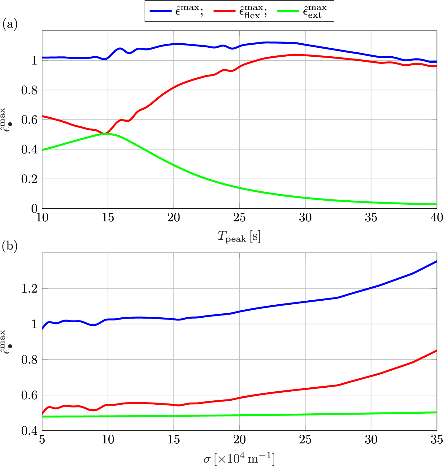
4.3 Time domain: parameter analysis
The maximum strain modulus (maximum of $\vert \epsilon \vert $
with respect to time and space) along the lower surface of a
$\vert \epsilon \vert $
with respect to time and space) along the lower surface of a $D=200$
m-thick ice shelf, induced by an incident wave packet, is similar to that of the corresponding frequency-domain problem over peak periods from 10 to 40 s, with the packet width held fixed at
$D=200$
m-thick ice shelf, induced by an incident wave packet, is similar to that of the corresponding frequency-domain problem over peak periods from 10 to 40 s, with the packet width held fixed at $\sigma =2\times 10^{-3}$
m
$\sigma =2\times 10^{-3}$
m $^{-1}$
, as shown by
$^{-1}$
, as shown by
 $$ \begin{align} {\hat{\epsilon}^{\max}\equiv \vert\hat{\epsilon}(x_{\max},t_{\max})\vert} \end{align} $$
as a function of $T_{\text {peak}}$
(Figure 6a). The contribution of flexural waves to the maximum strain is greater than that of extensional motions across the peak period range, as shown by
$T_{\text {peak}}$
(Figure 6a). The contribution of flexural waves to the maximum strain is greater than that of extensional motions across the peak period range, as shown by
 $$ \begin{align} {\hat{\epsilon}^{\max}_{\text{flex}}\equiv \vert\hat{\epsilon}_{\text{flex}}(x_{\max},t_{\max})\vert \quad\text{and}\quad \hat{\epsilon}^{\max}_{\text{ext}}\equiv \vert \hat{\epsilon}_{\text{ext}}(x_{\max},t_{\max})\vert} \end{align} $$
(Figure 6a), except for around the 15 s peak period where they are almost identical (see Figure 5c). The contribution to the maximum strain due to extensional waves attains its maximum around the 15 s peak period. It decreases slightly as the peak period decreases below $T_{\text {peak}}=15$
s and strongly as the peak period increases, such that flexural waves contribute
$T_{\text {peak}}=15$
s and strongly as the peak period increases, such that flexural waves contribute $>90$
% of the maximum strain for peak periods greater than 27 s.
$>90$
% of the maximum strain for peak periods greater than 27 s.
Maximum strain, $\hat {\epsilon }^{\max }$
(4.6), of a
$\hat {\epsilon }^{\max }$
(4.6), of a $D=200$
m-thick ice shelf, and corresponding strains due to flexural and extensional waves,
$D=200$
m-thick ice shelf, and corresponding strains due to flexural and extensional waves, $\hat {\epsilon }^{\max }_{\text {flex}}$
and
$\hat {\epsilon }^{\max }_{\text {flex}}$
and $\hat {\epsilon }^{\max }_{\text {ext}}$
(4.7), respectively, as functions of (a) peak period for wave packet width
$\hat {\epsilon }^{\max }_{\text {ext}}$
(4.7), respectively, as functions of (a) peak period for wave packet width $\sigma = 2\times 10^{-3}$
m
$\sigma = 2\times 10^{-3}$
m $^{-1}$
and (b) wave packet width
$^{-1}$
and (b) wave packet width $\sigma $
for peak period
$\sigma $
for peak period $T_{\text {peak}} = 15$
s.
$T_{\text {peak}} = 15$
s.

For a fixed peak period of $T_{\text {peak}}=15$
s, the maximum strain modulus increases with respect to that of the corresponding frequency-domain problem (that is,
$T_{\text {peak}}=15$
s, the maximum strain modulus increases with respect to that of the corresponding frequency-domain problem (that is, $\hat {\epsilon }^{\max }$
increases) as the packet width,
$\hat {\epsilon }^{\max }$
increases) as the packet width, $\sigma $
, increases (Figure 6b). The contribution due to flexural waves,
$\sigma $
, increases (Figure 6b). The contribution due to flexural waves, $\hat {\epsilon }^{\max }_{\text {flex}}$
, also increases with increasing packet width, but the contribution due to extensional waves,
$\hat {\epsilon }^{\max }_{\text {flex}}$
, also increases with increasing packet width, but the contribution due to extensional waves, $\hat {\epsilon }^{\max }_{\text {ext}}$
, is insensitive to the packet width. This is backed by the time series of the strains due to flexural and extensional waves,
$\hat {\epsilon }^{\max }_{\text {ext}}$
, is insensitive to the packet width. This is backed by the time series of the strains due to flexural and extensional waves, $\hat {\epsilon }_{\text {flex}}$
and
$\hat {\epsilon }_{\text {flex}}$
and $\hat {\epsilon }_{\text {ext}}$
, at the location of the maximum strain,
$\hat {\epsilon }_{\text {ext}}$
, at the location of the maximum strain, $x=x_{\max }$
(Figure 7). Increasing the packet width in the wavenumber (or frequency) domain, that is, increasing
$x=x_{\max }$
(Figure 7). Increasing the packet width in the wavenumber (or frequency) domain, that is, increasing $\sigma $
, results in a narrowing of the packet in the time domain. The maximum value of
$\sigma $
, results in a narrowing of the packet in the time domain. The maximum value of $\hat {\epsilon }_{\text {ext}}$
is unaffected by the packet width (Figure 7a), noting that the amplitude
$\hat {\epsilon }_{\text {ext}}$
is unaffected by the packet width (Figure 7a), noting that the amplitude $A_{0}$
scales with
$A_{0}$
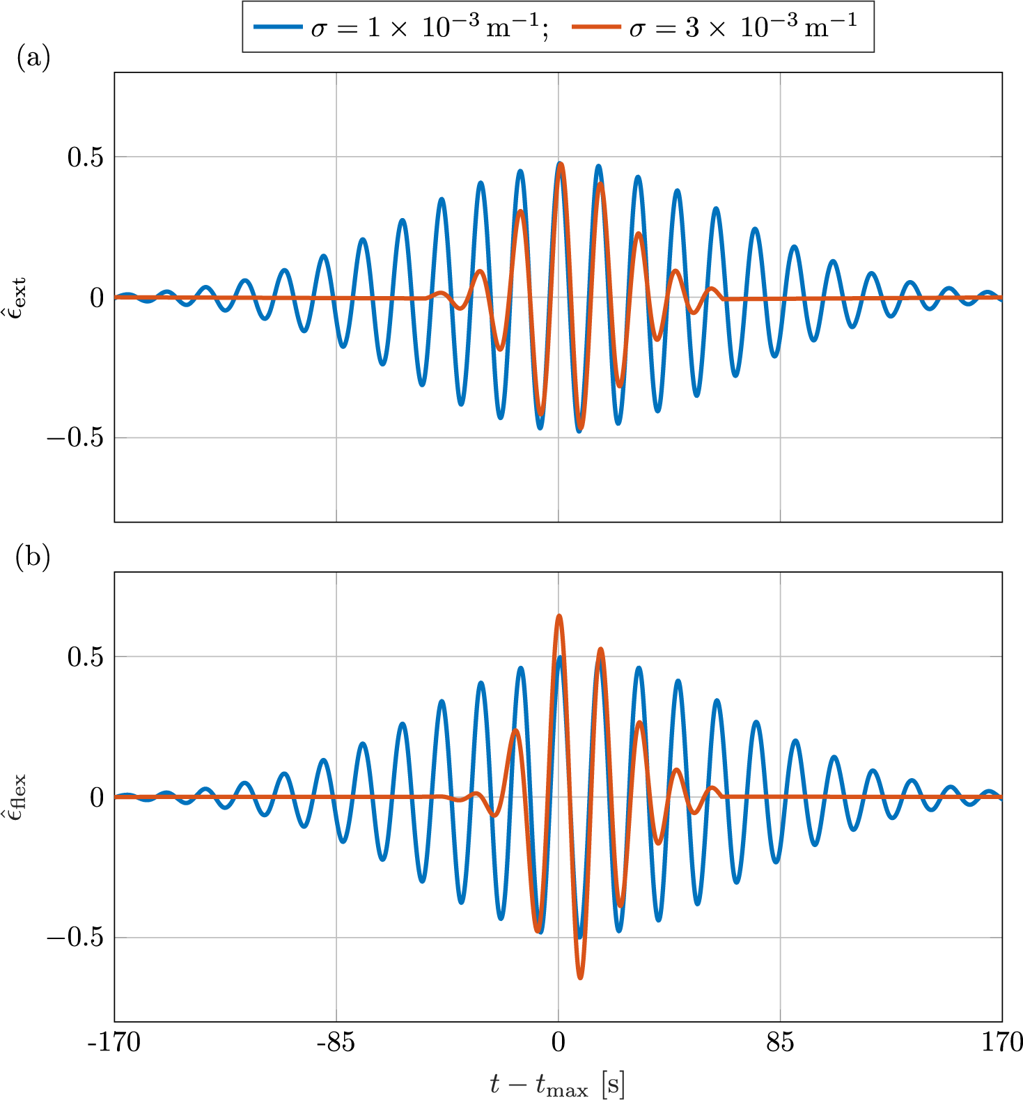
scales with $1/\sqrt {\sigma }$
to maintain a consistent energy and, thus, the smaller width produces a greater maximum value for the unnormalized strains. For the strain due to flexural waves, narrowing of the packet in the time domain is accompanied by an increase in the peak of
$1/\sqrt {\sigma }$
to maintain a consistent energy and, thus, the smaller width produces a greater maximum value for the unnormalized strains. For the strain due to flexural waves, narrowing of the packet in the time domain is accompanied by an increase in the peak of $\hat {\epsilon }_{\text {flex}}$
(Figure 7b).
$\hat {\epsilon }_{\text {flex}}$
(Figure 7b).
Time series of the strains on a $D=200$
m-thick ice shelf, due to (a) extensional waves,
$D=200$
m-thick ice shelf, due to (a) extensional waves, $\hat {\epsilon }_{\text {ext}}$
(4.4b), and (b) flexural waves,
$\hat {\epsilon }_{\text {ext}}$
(4.4b), and (b) flexural waves, $\hat {\epsilon }_{\text {flex}}$
(4.4a), at the location of the maximum strain,
$\hat {\epsilon }_{\text {flex}}$
(4.4a), at the location of the maximum strain, $x=x_{\text {max}}$
, caused by an incident wave packet of peak period
$x=x_{\text {max}}$
, caused by an incident wave packet of peak period $T_{\text {peak}}=15$
s and packet widths
$T_{\text {peak}}=15$
s and packet widths $\sigma = 1\times \,10^{-3}$
m
$\sigma = 1\times \,10^{-3}$
m $^{-1}$
(blue curves) and
$^{-1}$
(blue curves) and $\sigma = 3\times \,10^{-3}$
m
$\sigma = 3\times \,10^{-3}$
m $^{-1}$
(red).
$^{-1}$
(red).

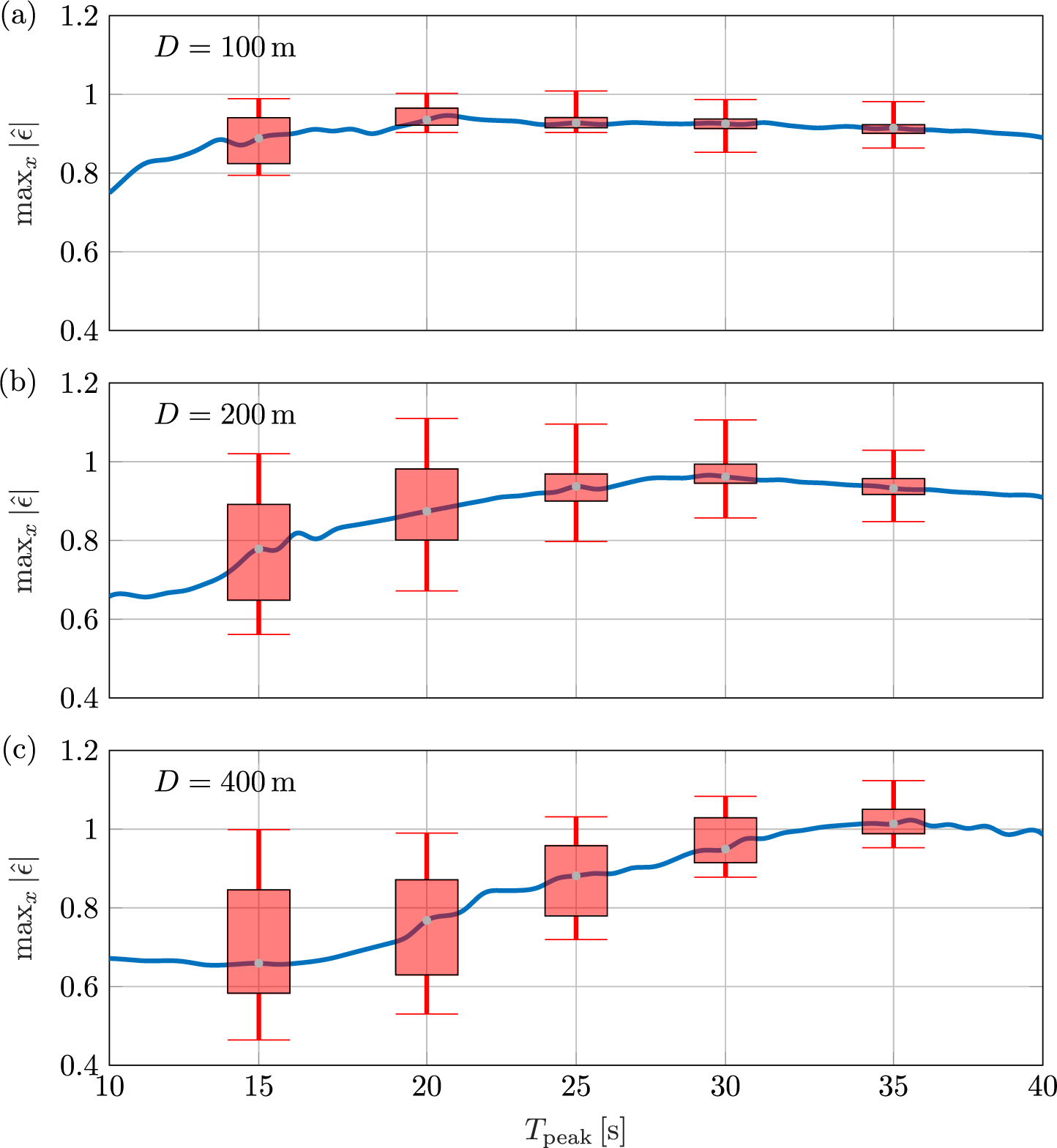
Statistics of $\max _{x}\hat {\epsilon }(x,t)$
versus peak period, with fixed packet width
$\max _{x}\hat {\epsilon }(x,t)$
versus peak period, with fixed packet width $\sigma = 2\times 10^{-3}$
m
$\sigma = 2\times 10^{-3}$
m $^{-1}$
for ice-shelf thickness (a)
$^{-1}$
for ice-shelf thickness (a) $D = 100$
m, (b)
$D = 100$
m, (b) $D=200$
m and (c)
$D=200$
m and (c) $D=400$
m. Median strains (blue curves) are shown at each peak period, along with interquartile ranges (boxes) and min–max values (whiskers) for subsets of peak periods, where statistics are for datasets over
$D=400$
m. Median strains (blue curves) are shown at each peak period, along with interquartile ranges (boxes) and min–max values (whiskers) for subsets of peak periods, where statistics are for datasets over $0<x<50$
km, from the time the incident packet peak reaches the shelf front to the time it reaches
$0<x<50$
km, from the time the incident packet peak reaches the shelf front to the time it reaches $x=50$
km, with data stored at spatial and temporal resolutions of 200 m and 2 s, respectively.
$x=50$
km, with data stored at spatial and temporal resolutions of 200 m and 2 s, respectively.

Extensional and flexural waves can interact coherently, which creates the maximum strains (for example, Figure 5c), and incoherently, which reduces the strains in relation to the individual extensional and flexural components of the strain field. Thus, for shorter peak periods, where strains have comparable contributions from flexural and extensional waves, there are relatively large spreads of
 $$ \begin{align*} { \max_{x}\vert\hat{\epsilon}\vert \quad\text{for } 0<x<50\text{\,km}, } \end{align*} $$
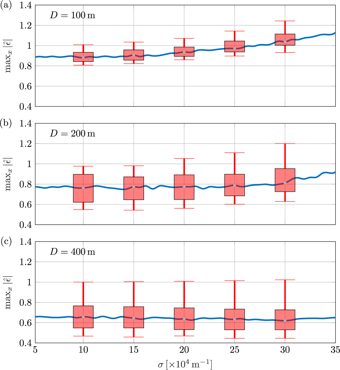
over a time interval for which the packet crosses that length of the ice shelf; whereas, at longer periods, where strains are dominated by flexural waves, distributions are far narrower (Figure 8). Thus, over the 10–40 s peak period interval shown, the median strain magnitude tends to increase with peak period for shorter peak periods and be relatively insensitive to peak period for longer peak periods. The transition between these regimes shifts to longer peak periods as the shelf thickness increases, as extensional waves make an appreciable contribution to strain up to longer periods for thicker ice shelves (see Figure 2a). In contrast, there is little variation in the spread of the (normalized) strain magnitudes with respect to the incident packet width (Figure 9).
As in Figure 8 but versus wave packet width, with peak period $T_{\text {peak}} = 15$
s.
$T_{\text {peak}} = 15$
s.

5 Conclusions
The flexural strain imposed on a floating ice shelf by an incident wave packet from the open ocean has been studied using a mathematical model in which the ice shelf is modelled as a thin plate that supports extensional waves in addition to flexural waves. In the wave period interval of interest (the swell regime), it was shown that the flexural and extensional waves generated in the ice shelf by the incident packet interact before they separate due to their different speeds. Coherent interactions create the largest ice-shelf strains, although these are accompanied by incoherent interactions that can reduce the strains. The maximum strains are comparable to, and usually slightly exceed, those predicted by a corresponding frequency-domain problem.
The findings support the conclusions of [Reference Bennetts, Williams and Porter10] on the importance of incorporating extensional waves into models when making predictions of the strains imposed on ice shelves by ocean swell. To be compatible with state-of-the-art predictions of the impacts of swell on Antarctic ice shelves [Reference Bennetts, Liang and Pitt8, Reference Liang, Pitt and Bennetts28, Reference Tazhimbetov, Almquist, Werpers and Dunham36], the model must be developed to incorporate spatial variations in the ice shelf geometry. The spatial variations should include ice shelf thickening away from the shelf front, which causes flexural waves to attenuate away from the shelf front [Reference Liang, Pitt and Bennetts28], so that the models can then test if attenuation of the extensional waves is significantly weaker, as observed on the Ross Ice Shelf [Reference Chen, Bromirski, Gerstoft, Stephen, Wiens, Aster and Nyblade14]. Models with spatial variations can also be used to test the effects of crevasses on ice shelf strain, noting that models involving only flexural waves predict that crevasses create local amplifications in strain forced by swell [Reference Bennetts, Liang and Pitt8].
Acknowledgements
This research was supported by the Australian Research Council (FT190100404). We thank the anonymous referees for their constructive comments. L. Bennetts thanks Andrew Bassom for the support and encouragement he has given over the past decade.
Appendix A Approximate solution: additional details
Solutions of the governing equations for flexural waves in the ice shelf–cavity region ((3.3b)–(3.3c)) are sought by writing
 $$ \begin{align} \psi(x)=c\,{e}^{{i}\lambda} \quad\text{and}\quad w(x)=\gamma\,{e}^{{i}\lambda}, \end{align} $$
where $\lambda $
, c and
$\lambda $
, c and $\gamma $
are to be found. Substituting (A.1) into ((3.3b)–(3.3c)) gives
$\gamma $
are to be found. Substituting (A.1) into ((3.3b)–(3.3c)) gives
 $$ \begin{align} a\,(\kappa^{2}-\lambda^{2})\,c - \kappa\,\tanh(\kappa\,H)\,c + \frac{\omega^{2}}{g}\,\gamma & = 0\quad \text{and} \end{align} $$
 $$ \begin{align} \{F\,\lambda^{4} - J\,\omega^{2}\,\lambda^{2} + 1-m\,\omega^{2}\}\,\gamma - c & = 0, \end{align} $$
where $b=\kappa ^{2}\,a-\kappa \,\tanh (\kappa \,H)$
has been used in (A.2a). Nontrivial solutions,
$b=\kappa ^{2}\,a-\kappa \,\tanh (\kappa \,H)$
has been used in (A.2a). Nontrivial solutions, $(c,\gamma )$
, of the system ((A.2a)–(A.2b)) exist if its determinant is zero, that is,
$(c,\gamma )$
, of the system ((A.2a)–(A.2b)) exist if its determinant is zero, that is,
 $$ \begin{align} \{ a\,(\kappa^{2}-\lambda^{2})-\kappa\,\tanh(\kappa\,H) \} \, \{F\,\lambda^{4} - J\,\omega^{2}\,\lambda^{2} + 1-m\,\omega^{2}\} + \frac{\omega^{2}}{g} = 0. \end{align} $$
Using the dispersion relation (3.2b) to replace the final term on the left-hand side of (A.3) and rearranging, gives
 $$ \begin{align} (\kappa^{2}-\lambda^{2}) \, [a\,\{F\,\lambda^{4} - J\,\omega^{2}\,\lambda^{2} + 1-m\,\omega^{2}\} + \{F\,(\kappa^{2}+\lambda^{2}) - J\,\omega^{2}\}\,\kappa\,\tanh(\kappa\,H)] = 0. \end{align} $$
Equation (A.4) is satisfied if $\lambda =\pm \kappa $
, in which case (A.2b) becomes
$\lambda =\pm \kappa $
, in which case (A.2b) becomes
 $$ \begin{align*} \{F\,\kappa^{4} - J\,\omega^{2}\,\kappa^{2} + 1-m\,\omega^{2}\}\,\gamma - c & = 0 \\ \Rightarrow \ \frac{\omega^{2}\,\gamma}{g\,\kappa\,\tanh(\kappa\,H)} -c & = 0, \end{align*} $$
from which (3.7) can be deduced. If $\lambda \neq \pm \kappa $
, then (A.4) requires the factor in square brackets on its left-hand side to be zero, that is, (3.6) holds with
$\lambda \neq \pm \kappa $
, then (A.4) requires the factor in square brackets on its left-hand side to be zero, that is, (3.6) holds with $\lambda =\kappa _{-j}$
. In this case, substituting (3.6) with
$\lambda =\kappa _{-j}$
. In this case, substituting (3.6) with $\kappa _{-j}=\lambda $
into (A.2b) gives
$\kappa _{-j}=\lambda $
into (A.2b) gives
 $$ \begin{align*} \{F\,(\kappa^{2}+\lambda^{2}) - J\,\omega^{2}\}\,\kappa\,\tanh(\kappa\,H)\,\gamma + a\,c = 0, \end{align*} $$
from which (3.8) can be deduced.


 Open access