


1. Introduction
A number of problems in geophysics, engineering and biology involve the spreading of a viscous fluid beneath a surface skin or crust. In some settings, the surface layer is distinct from the fluid, such as for geological intrusions (Bunger & Cruden Reference Bunger and Cruden2011; Michaut Reference Michaut2011; Michaut & Manga Reference Michaut and Manga2014; Michaut, Thiriet & Thorey Reference Michaut, Thiriet and Thorey2016), the production of silicon wafers (Huang & Suo Reference Huang and Suo2002a,Reference Huang and Suob), deformable channels in microfluidics (Hosoi & Mahadevan Reference Hosoi and Mahadevan2004; Kodio, Griffiths & Vella Reference Kodio, Griffiths and Vella2017), micro-scale lithography (Box et al. Reference Box, O'Kiely, Kodio, Inizan, Castrejón-Pita and Vella2019), airway reopening (Gaver et al. Reference Gaver, Halpern, Jensen and Grotberg1996; Jensen et al. Reference Jensen, Horsburgh, Halpern and Gaver2002; Grotberg & Jensen Reference Grotberg and Jensen2004) or in models of plant cell walls (Dyson & Jensen Reference Dyson and Jensen2010; Ali et al. Reference Ali, Mirabet, Godin and Traas2014). In others, the skin forms atop the flow as the fluid cools, solidifies, evaporates or reacts (Griffiths & Fink Reference Griffiths and Fink1993; Griffiths Reference Griffiths2000; Brož et al. Reference Brož, Krỳza, Wilson, Conway, Hauber, Mazzini, Raack, Balme, Sylvest and Patel2020).
A number of theoretical and experimental models of these flows have considered the skin layer to be a solid, thin, elastically deforming crust (e.g. Flitton & King Reference Flitton and King2004; Hosoi & Mahadevan Reference Hosoi and Mahadevan2004; Lister, Peng & Neufeld Reference Lister, Peng and Neufeld2013; Hewitt, Balmforth & De Bruyn Reference Hewitt, Balmforth and De Bruyn2015; Peng et al. Reference Peng, Pihler-Puzović, Juel, Heil and Lister2015; Pihler-Puzović et al. Reference Pihler-Puzović, Juel, Peng, Lister and Heil2015; Ball & Neufeld Reference Ball and Neufeld2018; Berhanu et al. Reference Berhanu, Guérin, Du Pont, Raoult, Perrier and Michaut2019; Pedersen et al. Reference Pedersen, Niven, Salez, Dalnoki-Veress and Carlson2019; Peng & Lister Reference Peng and Lister2020). The description of the skin and its restraining effect on the underlying fluid flow is then compactly described by coupling membrane, Euler–Bernoulli or Föppl–von-Kármán equations (Timoshenko & Woinowsky-Krieger Reference Timoshenko and Woinowsky-Krieger1959) for the skin with lubrication theory for the underlying viscous spreading. An important feature of the spreading dynamics in this problem is that it becomes limited by conditions at the periphery of the flow: although the spreading could potentially adopt a self-similar form (once the memory of the initial shape of a mound of fluid is lost, or the flow expands far beyond the radius of a vent through which the fluid is pushed, and there is no longer an intrinsic horizontal length scale), the singular nature of the contact line at the periphery prevents the convergence to such a state. Instead, the expansion is controlled by how the elastic sheet is ‘peeled off’ the underlying substrate by the viscous flow, becoming quasi-steady and constant pressure over the bulk of the viscous film (Flitton & King Reference Flitton and King2004; Lister et al. Reference Lister, Peng and Neufeld2013; Hewitt et al. Reference Hewitt, Balmforth and De Bruyn2015).
Although popular, an elastic skin is not the only possible model for the crust. Indeed, as often argued for lava flows (Griffiths & Fink Reference Griffiths and Fink1993; Griffiths Reference Griffiths2000; Castruccio, Rust & Sparks Reference Castruccio, Rust and Sparks2013), when the surface layer is a significantly broken-up solidified crust, other models may be more relevant, such as a substantially more viscous fluid, or a plastic material. The latter also applies when a solid crust is softer and forced to deform well beyond its yield point, but without fracture. Similarly, floating crusts of ice and other complex fluids (MacAyeal Reference MacAyeal1989; Feltham Reference Feltham2008; Schoof & Hewitt Reference Schoof and Hewitt2013; Sauret et al. Reference Sauret, Boulogne, Cappello, Dressaire and Stone2015; Sayag & Worster Reference Sayag and Worster2019) are typically neither elastic nor viscous.
In the current paper, we reconsider the problem of a viscous fluid spreading underneath a skin. We depart from previous analysis (e.g. Lister et al. Reference Lister, Peng and Neufeld2013; Hewitt et al. Reference Hewitt, Balmforth and De Bruyn2015; Peng & Lister Reference Peng and Lister2020) by adopting a model for the crust which allows that surface layer to deform either much more viscously than the underlying fluid, or as an ideal plastic solid. For this task, we employ a model for a viscoplastic plate which is derived from the governing equations of a material described by a standard non-Newtonian constitutive law, the Herschel–Bulkley law (Balmforth & Hewitt Reference Balmforth and Hewitt2013; Ball & Balmforth Reference Ball and Balmforth2021). The derivation of the plate model follows previous work for sheets of viscous fluid (Howell Reference Howell1996; Ribe Reference Ribe2001, Reference Ribe2002), and in certain limits can be reduced to that of a viscous fluid or ideal plastic material. The model therefore provides the viscoplastic analogue of the Föppl–von-Kármán plate equations, and connects viscous sheet models and classical theories of plastic plates (Prager & Hodge Reference Prager and Hodge1951; Hopkins & Prager Reference Hopkins and Prager1954; Hopkins & Wang Reference Hopkins and Wang1955; Hodge & Belytschko Reference Hodge and Belytschko1968; Lubliner Reference Lubliner2008), whilst further adding the effects of in-plane tensions to the latter. Our use of this viscoplastic model underscores a key simplification that we make, namely that we take the skin to be a materially distinct layer, not generated by solidification, reaction or evaporation. This simplification limits the application to situations in which the gradual thickening of the skin during spreading is not important.
Although we employ a different description for the plate, one of the questions we address is whether peeling at the contact line still impacts the spreading dynamics. We therefore adopt the common practice of regularizing the contact-line behaviour by pre-wetting the substrate with a thin film of viscous fluid. Viscous fluid is then introduced and driven underneath the plate through a source, our interest lying in the regime in which the resulting, spreading ‘blister’ is much deeper than the pre-wetted film. We explore in detail the peeling layer and confirm that it exerts the same control on spreading as when the skin is elastic.
From a mathematical perspective, the different form of the model for the viscoplastic plate over an elastic one leads to some novel features in the peeling dynamics. If the plate is purely viscous, it turns out that the peeling problem simplifies dramatically in comparison with the corresponding elastic analysis. This simplification arises because of the existence of an integral constant that permits one to avoid a detailed match between the main blister and the peeling layer. This simplification also features when the plate has a yield stress. However, understanding the spatial structure of the peeling layer is rather more challenging, as a convoluted sequence of interlaced plugs and yielded zones can arise in the plate, somewhat like in other problems with viscoplastic films (Jalaal & Balmforth Reference Jalaal and Balmforth2016; Jalaal, Stoeber & Balmforth Reference Jalaal, Stoeber and Balmforth2021).
2. Model equations
2.1. Governing equations
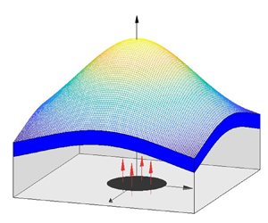
We model a thin plate of viscoplastic fluid satisfying the Herschel–Bulkley constitutive law lying above a shallow layer of viscous fluid flowing over a horizontal surface, as sketched in figure 1. Both fluids are incompressible. The thickness  ${\mathcal {D}}$ of the plate is comparable to the typical depth of the viscous fluid layer ${\mathcal {H}}$, but both are much smaller than the characteristic horizontal length scale ${\mathcal {L}}$
 \begin{equation} \epsilon=\frac{{\mathcal{H}}}{{\mathcal{L}}}\ll1, \quad \delta=\frac{{\mathcal{H}}}{{\mathcal{D}}}=O(1). \end{equation}
We use either a Cartesian coordinate system  $(x,y,z)$ or cylindrical polars $(r,\theta,z)$ to describe the geometry; the normal to the underlying plane points in the $z-$direction. The governing equations for an incompressible fluid with velocity field $\boldsymbol {u}$ are, discarding inertia,
 $$\begin{gather} \boldsymbol{\nabla} \boldsymbol{\cdot} \boldsymbol{u} = 0, \end{gather}$$
 $$\begin{gather}0 ={-}\boldsymbol{\nabla} p + \boldsymbol{\nabla}\boldsymbol{\cdot} \boldsymbol{\tau} + \rho {\boldsymbol{g}} , \end{gather}$$
where  ${\boldsymbol {g}}=(0,0,-g)$ is gravity, $\rho$ is the density of the fluid, $p$ is pressure and $\boldsymbol {\tau }$ is the deviatoric stress tensor.
A sketch of the model problem and its geometry: a thin viscoplastic plate is pushed upwards as a shallow film of viscous fluid is pumped underneath.

In the viscous fluid,  $\tau _{jk}=\mu {\dot {\gamma }}_{jk}$, where $\mu$ is the viscosity. For the plate, on the other hand, the Herschel–Bulkley constitutive law provides
 \begin{equation} \left.\begin{array}{ll@{}}
\boldsymbol{\dot{\gamma}} =\boldsymbol{0}, & \tau<{{\tau_{Y}}},\\
\boldsymbol{\tau}
=\left(K{\dot{\gamma}}^{n-1}+\dfrac{{{\tau_{Y}}}}{\dot{\gamma}}\right)\boldsymbol{\dot{\gamma}},
& \tau\geq {{\tau_{Y}}}, \end{array}\right\}
\end{equation}
\begin{equation} \left.\begin{array}{ll@{}}
\boldsymbol{\dot{\gamma}} =\boldsymbol{0}, & \tau<{{\tau_{Y}}},\\
\boldsymbol{\tau}
=\left(K{\dot{\gamma}}^{n-1}+\dfrac{{{\tau_{Y}}}}{\dot{\gamma}}\right)\boldsymbol{\dot{\gamma}},
& \tau\geq {{\tau_{Y}}}, \end{array}\right\}
\end{equation}
where  ${{\tau _{Y}}}$, $K$ and $n$ represent the yield stress, consistency and power-law index, and
 \begin{equation} {\dot{\gamma}}_{jk} = \frac{\partial u_j}{\partial x_k} + \frac{\partial u_k}{\partial x_j} , \quad {\dot{\gamma}} = \sqrt{\frac{1}{2}\sum_{j,k}{\dot{\gamma}}_{jk}^2}, \quad \tau = \sqrt{\frac{1}{2}\sum_{j,k}\tau_{jk}^2} . \end{equation}
For  ${{\tau _{Y}}}\to 0$, the Herschel–Bulkley law reduces to that for a power-law fluid (and a viscous one if, further, $n=1$); when the yield stress dominates over the rate-dependent viscous component of the stresses, the model is equivalent to a perfectly plastic material described by the von Mises yield condition.
The densities of the viscous fluid and plate are not necessarily the same;  $\rho =\rho _f$ denotes the density of the viscous fluid, whereas $\rho =\rho _p$ is that of the plate. At the interface between the two fluids, $z=h({\boldsymbol {x}},t)$, we apply the usual kinematic condition and demand that stresses are continuous, ignoring any interfacial tension.
2.2. Lubrication theory for the viscous fluid
Because the fluid layer underneath the plate is relatively shallow, we exploit the lubrication approximation to describe the flow dynamics. In this approximation, the pressure becomes hydrostatic and drives a flow underneath the plate with a Poiseuille-type velocity profile that is  $O(\epsilon ^{-1})$ larger than the vertical velocity. Importantly, lubrication pressures far exceed viscous shear stresses, implying that the normal force exerted by the fluid on the plate is primarily generated by that pressure, and that the underlying viscous flow is not strong enough to provide a significant traction on the lower side of the plate. The plate therefore deforms mainly in the transverse (i.e. $z$) direction with a relatively weak in-plane velocity. In particular if ${\mathcal {V}}$ denotes a characteristic vertical velocity, the horizontal velocities of the plate are $O(\epsilon {\mathcal {V}})$.
Given these considerations, we follow conventional lubrication theory and use the depth-integrated mass conservation equation to derive a dimensionless evolution equation for the local fluid depth,
 \begin{equation} \frac{\partial h}{\partial t} = \boldsymbol{\nabla} \boldsymbol{\cdot}(h^3 \boldsymbol{\nabla}p) + {\rm source}. \end{equation}
To arrive at this dimensionless form, the local fluid depth is scaled by  ${\mathcal {H}}$, horizontal lengths by ${\mathcal {L}}$, time by ${\mathcal {H}}/{\mathcal {V}}$ and pressure with the scale,
 \begin{equation} {\mathcal{N}} = \frac{12\mu{\mathcal{L}}^2{\mathcal{V}}}{{\mathcal{H}}^3}, \end{equation}
which render  $h$ and $p$ as new dimensionless variables (avoiding any corresponding notation changes). The term written as $source$ denotes the dimensionless vertical velocity above the vent, where the viscous fluid is fed underneath the plate. If $P$ denotes the dimensionless fluid pressure on the underside of the plate, then
 \begin{align} p = P + {\mathcal{G}}(h-z) \quad {\rm or}\quad \boldsymbol{\nabla} p = \boldsymbol{\nabla} P + {\mathcal{G}} \boldsymbol{\nabla} h, \end{align}
where
 \begin{equation} {\mathcal{G}}=\frac{\rho_f g {\mathcal{H}}}{{\mathcal{N}}} \end{equation}
characterizes the influence of gravity on the blister. Practically, we take the scales  ${\mathcal {L}}$ and ${\mathcal {V}}$ to be prescribed by the size and flow speed associated with the vent.
As mentioned earlier, we demand that there is a thin film of viscous fluid everywhere underneath the viscoplastic plate with  $h=h_0$; i.e. we pre-wet the underlying plane with viscous fluid, following common practice in thin-film theory. This device allows us to avoid any potential problems in dealing with a true contact line (a triple-phase contour where the two fluids and substrate meet one another). In line with the introduction of this thin film to ‘regularize’ the problem, we consider the limit in which its thickness is small: $h_0\ll 1$.
2.3. Viscoplastic plate model
The lubrication pressure built up underneath the plate forces this skin to deflect upwards. As shown in Ball & Balmforth (Reference Ball and Balmforth2021), provided the plate is thin, the local thickness  ${\mathcal {D}}$ does not change to leading order, and a combination of bending stresses and in-plane tensions oppose deformation. The centreline of the plate then lies at ${\mathcal {H}} Z=\frac{1}{2} {\mathcal {D}}+{\mathcal {H}} h$, and $W=Z_t=h_t$ denotes the dimensionless vertical plate velocity.
The analysis in Ball & Balmforth (Reference Ball and Balmforth2021) indicates that the stresses developed in the plate are  $O({\mathcal {P}})$, where
 \begin{equation} {\mathcal{P}} = K \left( \frac{{\mathcal{D}}{\mathcal{V}}}{{\mathcal{L}}^2} \right)^n . \end{equation}
(Note that in Ball & Balmforth (Reference Ball and Balmforth2021) there is no viscous fluid layer underneath the plate, and we took the vertical length scale to be  ${\mathcal {D}}$.) These stresses generate a normal force on the plate of $O({\mathcal {P}}{\mathcal {D}}^2/{\mathcal {L}}^2)$ that counters the load exerted by the fluid pressure ${\mathcal {N}} P$ from below. As these must balance, we take
 \begin{equation} {\mathcal{N}}=\frac{{\mathcal{P}}{\mathcal{D}}^2}{{\mathcal{L}}^2}, \quad {\rm or} \quad {\mathcal{H}}=\left(\frac{12\mu{\mathcal{L}}^{2(2+n)}}{K{\mathcal{D}}^{2+n}{\mathcal{V}}^{n-1}}\right)^{1/3}, \end{equation}
which gauges the depth of the blister forced by the influx of viscous fluid.
The main thrust of the reduction in Ball & Balmforth (Reference Ball and Balmforth2021) is to express the force balance on the plate in terms of the bending moments and in-plane tensions that result from these stresses, and to relate those moments and tensions to  ${\mathcal {V}} W$ and the (suitably scaled) in-plane velocity $({\mathcal {H}}/{\mathcal {L}}){\mathcal {V}} {\boldsymbol {U}}$ through constitutive relations that descend from the original Herschel–Bulkley law. The constitutive laws are written in terms of the rates of curvature and in-plane extension, which in dimensional form are $({{\mathcal {V}}}/{{\mathcal {L}}^2}){\boldsymbol {K}}$ and $({{\mathcal {V}}{\mathcal {D}}}/{{\mathcal {L}}^2}){{\boldsymbol {D}}}$. The corresponding dimensionless rates are given by the tensors, ${\boldsymbol {K}} = \boldsymbol {\nabla }\boldsymbol {\nabla } W$ and ${{\boldsymbol {D}}}=\frac{1}{2}\delta (\boldsymbol {\nabla } {\boldsymbol {U}}+\boldsymbol {\nabla }{\boldsymbol {U}}^T + \boldsymbol {\nabla } h^T \boldsymbol {\nabla } W + \boldsymbol {\nabla } W^T \boldsymbol {\nabla } h)$, in Cartesian coordinates, or
 \begin{align} {\boldsymbol{K}} =
\left(\begin{array}{@{}cc@{}} W_{rr} & (r^{{-}1} W_{\theta})_r
\\ (r^{{-}1} W_{\theta})_r & r^{{-}2} W_{\theta\theta}+
r^{{-}1} W_r \end{array} \right) \end{align}
\begin{align} {\boldsymbol{K}} =
\left(\begin{array}{@{}cc@{}} W_{rr} & (r^{{-}1} W_{\theta})_r
\\ (r^{{-}1} W_{\theta})_r & r^{{-}2} W_{\theta\theta}+
r^{{-}1} W_r \end{array} \right) \end{align}
and
 \begin{align} {{\boldsymbol{D}}} = \delta \left( \begin{array}{@{}cc@{}} U_r + h_r W_r & \frac{1}{2} r^{{-}1}(U_\theta-rV_r-V + Z_\theta W_r + Z_r W_\theta) \\ \frac{1}{2} r^{{-}1}(U_\theta-rV_r-V + Z_\theta W_r + Z_r W_\theta) & r^{{-}1} (U+V_\theta) + r^{{-}2} Z_\theta W_\theta \end{array} \right) \end{align}
in polar form, where  ${\boldsymbol {U}} = (U,V)$.
The dimensional bending moments and tensions are  ${\mathcal {D}}^2{\mathcal {P}}{\boldsymbol {M}}$ and ${\mathcal {D}}{\mathcal {P}}\boldsymbol {\varSigma }$, where, over the sections where the plate is yielded,
 \begin{align} {\boldsymbol{M}} &= \varGamma^{n-1} \{ ( \varUpsilon I_{0,n}- I_{1,n}) \boldsymbol{\varDelta} + [2 \varUpsilon I_{1,n} - I_{0,n+2} + (\alpha^2-\varUpsilon^2) I_{0,n}] {\boldsymbol{\varGamma}} \} \nonumber\\ &\quad +\frac{{\textit{Bi}}}{\varGamma} \{ ( \varUpsilon I_{0,0}- I_{1,0}) \boldsymbol{\varDelta} + [2 \varUpsilon I_{1,0} - I_{0,2} + (\alpha^2-\varUpsilon^2) I_{0,0}] {\boldsymbol{\varGamma}} \}, \end{align}
 \begin{align} \boldsymbol{\varSigma} &=\varGamma^{n-1} [ I_{0,n} \boldsymbol{\varDelta} + (I_{1,n} - \varUpsilon I_{0,n})){\boldsymbol{\varGamma}} ] + \frac{{\textit{Bi}}}{\varGamma} [ I_{0,0} \boldsymbol{\varDelta} + (I_{1,0}- \varUpsilon I_{0,0}) {\boldsymbol{\varGamma}}] , \end{align}
with
 $$\begin{gather} {\boldsymbol{\varGamma}} = 2{\boldsymbol{K}} + 2\,{{\rm Tr}}({\boldsymbol{K}}){\bf I} , \quad \boldsymbol{\varDelta} = 2{{\boldsymbol{D}}} + 2\,{{\rm Tr}}({{\boldsymbol{D}}}){\bf I}, \end{gather}$$
 $$\begin{gather}\varGamma^2= \tfrac{1}{2}[ {{\rm Tr}}({{\boldsymbol{\varGamma}}}^2) - \tfrac{1}{3} {{\rm Tr}}({{\boldsymbol{\varGamma}}})^2 ], \quad \varUpsilon = \frac{{{\rm Tr}}(\boldsymbol{\varDelta} {\boldsymbol{\varGamma}})-\frac13{{\rm Tr}}(\boldsymbol{\varDelta}){{\rm Tr}}({\boldsymbol{\varGamma}})}{2\varGamma^2}, \end{gather}$$
 $$\begin{gather}\alpha^2 = \frac{{{\rm Tr}}(\boldsymbol{\varDelta}^2)-\frac13{{\rm Tr}}(\boldsymbol{\varDelta})^2}{2\varGamma^2} - \varUpsilon^2 \end{gather}$$
and
 \begin{equation} I_{j,n}(\alpha,\varUpsilon)= \int_{{-}1/2}^{1/2} (\varUpsilon-z)^j[(z-\varUpsilon)^2+\alpha^2]^{({n-1})/{2}} \,\mathrm{d}z . \end{equation}
We refer to the dimensionless yield stress parameter,
 \begin{equation} {\textit{Bi}}=\frac{{\tau_{Y}}}{\mathcal{P}} = \frac{{{\tau_{Y}}}}{K}\left(\frac{{\mathcal{L}}^2}{{\mathcal{D}}{\mathcal{V}}}\right)^n , \end{equation}
as the Bingham number. If the plate is not locally yielded, then  $\varGamma =0$. The original yield condition, $\tau ={{\tau _{Y}}}$, descends to the relations,
 \begin{equation} \left.\begin{gathered}
\varSigma^2 = {\textit{Bi}}^2 ( \alpha^2 I_{0,0}^2 +
I_{1,0}^2), \quad {\mathcal{X}} = {\textit{Bi}}^2
(\alpha^2 \varUpsilon I_{0,0}^2 + \varUpsilon
I_{1,0}^2 - I_{1,0} I_{0,2}),\\ M^2 =
{\textit{Bi}}^2 [\alpha^2(I_{1,0} - \varUpsilon
I_{0,0})^2 + ( I_{0,2} - \varUpsilon I_{1,0} - \alpha^2
I_{0,0} )^2],
\end{gathered}\right\}\end{equation}
\begin{equation} \left.\begin{gathered}
\varSigma^2 = {\textit{Bi}}^2 ( \alpha^2 I_{0,0}^2 +
I_{1,0}^2), \quad {\mathcal{X}} = {\textit{Bi}}^2
(\alpha^2 \varUpsilon I_{0,0}^2 + \varUpsilon
I_{1,0}^2 - I_{1,0} I_{0,2}),\\ M^2 =
{\textit{Bi}}^2 [\alpha^2(I_{1,0} - \varUpsilon
I_{0,0})^2 + ( I_{0,2} - \varUpsilon I_{1,0} - \alpha^2
I_{0,0} )^2],
\end{gathered}\right\}\end{equation}
where the three invariants,
 $$\begin{gather} M^2=\tfrac{1}{2}[{\rm Tr}({\boldsymbol{M}}^2)-\tfrac{1}{3}{\rm Tr}({\boldsymbol{M}})^2],\quad \varSigma^2 =\tfrac{1}{2}[{{\rm Tr}}(\boldsymbol{\varSigma}^2)-\tfrac{1}{3}{{\rm Tr}}(\boldsymbol{\varSigma})^2], \end{gather}$$
 $$\begin{gather}{\mathcal{X}} = \tfrac{1}{2}[{{\rm Tr}}({\boldsymbol{M}}\boldsymbol{\varSigma})-\tfrac{1}{3}{{\rm Tr}}({\boldsymbol{M}}){{\rm Tr}}(\boldsymbol{\varSigma})]. \end{gather}$$
 In the absence of inertia and any interfacial tensions, the force balance on the plate demands that  $\boldsymbol {0} = \boldsymbol {\nabla } \boldsymbol {\cdot } \boldsymbol {\varSigma }$ and $0=\boldsymbol {\nabla }\boldsymbol {\cdot }[\boldsymbol {\nabla }\boldsymbol {\cdot }({\boldsymbol {M}}+\delta h\boldsymbol {\varSigma } )] - ({\rho _p }/{\rho _f}){\mathcal {G}} + P$ (in Cartesian coordinates), or
 $$\begin{gather} 0=\frac{\partial}{\partial r}\varSigma_{rr} +\frac{1}{r}\frac{\partial}{\partial \theta}\varSigma_{r\theta} +\frac{1}{r}(\varSigma_{rr}-\varSigma_{\theta\theta}), \end{gather}$$
 $$\begin{gather}0=\frac{1}{r^2} \frac{\partial}{\partial r}(r^2 \varSigma_{r\theta}) +\frac{1}{r}\frac{\partial}{\partial \theta}\varSigma_{\theta\theta} , \end{gather}$$
 \begin{gather} 0 = \frac{1}{r^2} \frac{\partial}{\partial r} \left(r^2\frac{\partial M_{rr}}{\partial r}\right) +\frac{2}{r^2}\frac{\partial^2}{\partial r\partial\theta}(r M_{r\theta}) +\frac{1}{r^2}\frac{\partial^2M_{\theta\theta}}{\partial \theta^2} -\frac{1}{r}\frac{\partial M_{\theta\theta}}{\partial r} \nonumber\\ +\delta \left[h_{rr}\varSigma_{rr} +2\left(\frac{h}{r}\right)_{r\theta}\varSigma_{r\theta} +\frac{1}{r}\left(h_r+\frac{1}{r}h_{\theta\theta}\right) \varSigma_{\theta\theta}\right] -\frac{\rho_p}{\rho_f}{\mathcal{G}}+P \end{gather}
(in polar form).
3. Planar blisters
In the planar problem, the horizontal force balance on the plate reduces to  $\partial \varSigma _{xx}/\partial x=0$, highlighting how the viscous traction exerted on the plate by the fluid underneath is too small to appear in lubrication theory. Hence, if the plate is free at its edges, it is not possible to build up an appreciable tension. The plate model then simplifies substantially ( $(\varDelta _{xx},\varUpsilon,\alpha )\to 0$) to furnish the problem,
 $$\begin{gather} \frac{\partial h}{\partial t} = W , \end{gather}$$
 $$\begin{gather}W = \frac{\partial}{\partial x}\left[ h^3 \frac{\partial }{\partial x}\left( P + {\mathcal{G}} h \right)\right] + {\rm source}, \end{gather}$$
 $$\begin{gather}\frac{\partial^2 M_{xx}}{\partial x^2} + P = {\mathcal{G}} \frac{\rho_p}{\rho_f}, \end{gather}$$
 $$\begin{gather}\frac{\partial^2 W}{\partial x^2} ={-} \left[ (n+2) \, {\rm Max}(|M_{xx}| - \frac{1}{2}{\textit{Bi}},0 ) \right]^{1/n} \, {\rm sgn}(M_{xx}) . \end{gather}$$
The plate is yielded when  $|M_{xx}|>{\textit {Bi}}/2$, and $\partial ^2 W/\partial x^2=0$ otherwise. Symmetry demands that
 \begin{equation} \frac{\partial W}{\partial x} = \frac{\partial }{\partial x}M_{xx} = \frac{\partial P}{\partial x} = 0 \quad {\rm at} \ x=0. \end{equation}
Away from the pumped-up blister, the plate rests on the pre-wetted film, so that
 \begin{equation} \left(W , \frac{\partial W}{\partial x}, \frac{\partial P}{\partial x}\right) \to 0 \quad {\rm for} \ x\gg1 . \end{equation}
To model the influx of viscous fluid, we set
 \begin{equation} {\rm source} = \left\{
\begin{array}{@{}ll} 1-x^2, & |x|<1 \\ 0, & |x |>1 \end{array}
\right. . \end{equation}
\begin{equation} {\rm source} = \left\{
\begin{array}{@{}ll} 1-x^2, & |x|<1 \\ 0, & |x |>1 \end{array}
\right. . \end{equation}
Practically, we solve the system in (3.1)–(3.4) for a Bingham plate numerically starting with the initial condition  $h(x,0)=h_0$. We adopt a finite spatial domain of length $L$, with $L$ mostly chosen sufficiently large that the far boundary remains sufficiently distant to have no effect on the results (see Appendix B). The numerical scheme constructs the instantaneous vertical velocity $W$ and depth $h(x,t)$ at each moment in time by solving (3.2)–(3.4) as a boundary-value problem in space using MATLAB's built-in solver bvp4c, given the simple finite difference scheme for (3.1),
 \begin{equation} h(x,t) = h(x,t-{\rm d} t) + \tfrac{1}{2} {\rm d} t[ W(x,t) + W(x,t-{\rm d} t)], \end{equation}
together with the previous pair,  $h(x,t-\textrm {d} t)$ and $W(x,t-\textrm {d} t)$, and a suitably chosen, small time step $\textrm {d} t$. To ease the computations with ${\textit {Bi}}>0$, we also smooth the switch in (3.4) by introducing the replacement,
 \begin{equation} M_{xx} ={-} \left[ \frac{1}{3}+\frac{1}{2}{\textit{Bi}}\left(\left|\frac{\partial^2 W}{\partial x^2}\right| +\epsilon\right)^{{-}1}\right]\frac{\partial^2 W}{\partial x^2}, \end{equation}
which can be inverted to give
 \begin{gather} \frac{\partial^2 W}{\partial x^2}={-}\left[\frac14(6|M_{xx}|-3{\textit{Bi}}-2\epsilon) +\frac14\sqrt{(6|M_{xx}|-3{\textit{Bi}}-2\epsilon)^2+48\epsilon|M_{xx}|}\right] \mathrm{sgn}(M_{xx}). \end{gather}
The value of  $\epsilon$ is taken to be sufficiently small to ensure that the main details of the blisters are independent of the precise value of this parameter. However, as we argue below, it is not possible to fully divorce the structure of the solution from this regularization parameter (see, again, Appendix B).
Because the underlying plane is everywhere separated from the plate by the pre-wetted film, there is no true contact line at the edge of the pumped-up blister. Instead, we define an effective edge using the first position  $x=X_e(t)$ that the fluid depth reaches the pre-wetted film thickness; i.e. $h(X_e,t)=h_0$.
3.1. Viscous beam  ${\textit {Bi}}=0$

When the plate is purely viscous ( ${\textit {Bi}}=0; n=1$), further simplifications result in
 \begin{equation} W = \frac{\partial}{\partial x} \left[ h^3 \left(\frac{\partial P}{\partial x} + {\mathcal{G}} \frac{\partial h}{\partial x} \right)\right] + {\rm source}, \quad P=\frac{1}{3}\frac{\partial^4 W}{\partial x^4}, \quad \frac{\partial h}{\partial t} = W . \end{equation}
The version of this viscous model in which the gravitational term dominates the bending term in the evolution equation is well known (e.g. Huppert Reference Huppert1982), so we consider the opposite limit by taking  ${\mathcal {G}}\to 0$. In view of scalings, and with the restriction to the Bingham case, this parameter is given more explicitly by
 \begin{equation} {\mathcal{G}} = \frac{\rho_f g {\mathcal{L}}^6 (12\mu)^{1/3}}{{\mathcal{V}} {\mathcal{D}}^4~K^{4/3}}. \end{equation}
3.1.1. Numerical results
A numerical solution to (3.11a–c) for  ${\mathcal {G}}=0$ is shown in figure 2. Once pumping commences a blister rises up above the vent (spanning $|x|<1$). The blister then expands sideways as the less viscous fluid from the vent is driven under the much more viscous plate. As observed in spreading flow underneath elastic sheets, the blister quickly settles into a quasi-steady shape in which the fluid pressure is almost uniform, with the overlying skin evolving in the same manner as a viscous beam under a spatially uniform, time-dependent load (cf. the ‘glass-blowing’ solutions of Ribe (Reference Ribe2001)). At this stage, the expansion is controlled by a thin layer at the edge over which the viscous plate is peeled off the pre-wetted film and pressure gradients become significant. The figure shows details of the main blister, as well as the peeling layer. Time series of some of the global features of the blister are plotted in figure 3, for both the solution shown in figure 2 and more solutions with varying $h_0$. Plotted, in particular, are the maximum depth
 \begin{equation} h_{max}(t)=h(0,t), \end{equation}
edge position  $X_e(t)$ and central vertical velocity and pressure, $W(0,t)$ and $P(0,t)$. These attributes can be predicted by the matched asymptotic analysis of the blister and peeling layer; see § 3.1.2.
Numerical solution for a planar Newtonian plate ( ${\textit {Bi}}=0, n=1$) with $h_0=10^{-2}$ and $L=50$. (a) Evolution of the height of the blister. The red line indicates the blister's edge $X_e(t)$. Also shown are snapshots of (b) vertical velocity $W$, (c) pressure $P$ and (d) moment $M_{xx}$ at the times indicated and colour coded accordingly. The dashed lines plot the asymptotic solution for the blister from § 3.1.2. The inset in (c) shows the almost uniform interior pressure. Insets in (b,d) show a collapse of profiles in the peeling boundary layer when replotted using the scaled variables, $\xi =(x-X_e)/L_p$ and $f=h/h_0$, defined in (3.19a–d). The dot-dashed black lines plot the numerical solution to the peeling equation (3.20).

Time series of (a) maximum height  $h_{max}(t)$ and edge position $X_e(t)$, and (b) central vertical velocity and pressure, $W(0,t)$ and $P(0,t)$, for a planar Newtonian plate ( ${\textit {Bi}}=0$, $n=1$ and $L=50$) with differing pre-wetted layer thicknesses ( $h_0=(0.5, 1, 2, 4, 8)\times 10^{-2}$). The arrows in (a,b) show the trends with increasing $h_0$.

Figure 4 shows solutions for some variations on the basic spreading problem, namely for blisters in which the plate is terminated closer to the source, or when the pumping is turned off after a time  $t=t_s$. The blisters under a shorter plate reach the edges after an initial period of expansion, the peeling layer then stops advancing, prompting a faster growth of the thickness. In fact, since the pressure becomes largely uniform, the second relation in (3.11a–c), along with the boundary condition and unit flux, predicts that
 \begin{equation} W\sim \frac{5}{4L}\left(1-\frac{x^2}{L^2}\right)^2 \quad \text{and} \quad h\sim \frac{5t}{4L}\left(1-\frac{x^2}{L^2}\right)^2 , \end{equation}
in agreement with the numerical solutions in figure 4. When the pump rate is terminated after  $t=t_s$, the solution quickly converges to a steady state with $P=0$ throughout. The blister then largely remains at the shape it possessed when pumping ceased, because there is no levelling by gravity or interfacial tension. The final shape is now given by the peeling analysis, described next.
Numerical solutions for a planar Newtonian plate in which the edges  $x=\pm L$ are closer to the vent or pumping ceases at $t=t_s$ (with $h_0=10^{-2}$ and $L=50$). Shown are (a–c) surface plots of $h(x,t)$ above the $(x,t)$-plane, with red lines indicating the blister's edge $X_e(t)$. Also shown are time series of (d) $X_e(t)$ and (e) $h_{max}(t)$ and $W(0,t)$. The solution from figure 2 is shown in (a) and by the solid blue lines in (d,e). The other two surface plots show solutions with (b) $L=3$ and (c) $t_s=50$. Panels (d,e) show solutions with $L=1.3$, 2 and 3 (green dashed lines) and $t_s=1$, 5 and 20 (red dotted lines). The blue stars and red triangles indicate the predictions of the peeling analysis in § 3.1.2 (with $t\equiv t_s$ for the latter); the green triangles show the predictions in (3.14a,b). The insets show the final snapshots of the solutions in (d,e), with the small filled circles indicating $x=X_e(t)$, and the faint grey lines in the inset in (e) showing the evolution of $h(x,t)$ for the solution of figure 2.

3.1.2. Peeling analysis
When the pressure becomes approximately uniform,  $P\approx P(t)$, over the bulk of the blister, the quasi-static evolution of the shape is dictated by
 \begin{equation} P(t) \sim \frac{1}{3}\frac{\partial^4 W}{\partial x^4} , \end{equation}
subject to the symmetry conditions  $\partial W/\partial x=\partial ^3 W/\partial x^3=0$ at $x=0$. At the edge, $x\to X_e(t)$, the condition $h\rightarrow h_0$ must be supplemented with further conditions reflecting how the blister matches with the peeling layer. In particular, as indicated below, the peeling layer possesses a much shorter spatial scale than the main blister. The mismatch in first derivatives then demands that $\partial W / \partial x \to 0$ for $x\to X_e$, leaving a further condition to be imposed on $\partial ^2 W / \partial x^2$ that we identify below. All this parallels the analysis required for an elastic skin (Lister et al. Reference Lister, Peng and Neufeld2013; Hewitt et al. Reference Hewitt, Balmforth and De Bruyn2015).
An additional constraint on the main blister arises from mass conservation,
 \begin{equation} \tfrac{2}{3}t \sim \int_0^{X_e} ( h-h_0 ) \, {\rm d}\kern 0.06em x \quad {\rm or} \quad \tfrac{2}{3} \sim \int_0^{X_e} W \, {\rm d}\kern 0.06em x. \end{equation}
Hence,
 \begin{equation} W \sim \frac{5}{4X_e}\left(1-\frac{x^2}{X_e^2}\right)^2, \end{equation}
and so the blister has a curvature rate of
 \begin{equation} \left. \frac{\partial^2 W}{\partial x^2}\right|_{x\to X_e} \sim \frac{10}{X_e^3} \end{equation}
at the edge.
In the peeling layer, the solution takes the form of a travelling wave with
 \begin{equation} h \sim h_0f(\xi), \quad W \sim{-}\frac{\dot{X}_eh_0}{L_p} f'(\xi), \quad \xi = \frac{x-X_e(t)}{L_p}, \quad L_p=\left(\frac{1}{3} h_0^3\right)^{1/6}\ll1, \end{equation}
where (from (3.11a–c), given  $f\to 1$ for $\xi \to \infty$)
 \begin{equation} f - 1 = f^3f^{VI}. \end{equation}
This equation can be solved numerically, enforcing three boundary conditions on the right, to ensure that  $f\to 1$ for $\xi \to \infty$. To the left, we must impose conditions guided by matching: the solution for the main blister possesses derivatives that are $O(1)$ for $x\to X_e$. But the scaling of the peeling solution indicates that $\partial ^2 W/\partial x^2 \to - \dot {X}_e h_0 f''' / L_p^3 = O(1)$, whereas $\partial ^m W/\partial x^m=O(h_0^{1-{m}/{2}})$, which is small for $m=1$ and large for $m>2$. Hence to accomplish the match we must impose $\partial W/\partial x = 0$ at $x\to X_e$ for the main blister solution (as noted earlier), and eliminate the higher derivatives of the peeling-layer solution, corresponding to the conditions $(f^{IV}, f^V)\to 0$ for $\xi \to -\infty$. A sixth condition (such as $f=1$ at the right-hand point of the computational domain) is required to eliminate the translational invariance of (3.20).
This construction furnishes a solution for the peeling region, which, in principle, then provides a matching condition for the edge curvature in (3.18). However, unlike in other peeling problems (e.g. Flitton & King Reference Flitton and King2004; Lister et al. Reference Lister, Peng and Neufeld2013; Hewitt et al. Reference Hewitt, Balmforth and De Bruyn2015), the peeling equation in (3.20) has an even number of derivatives, which implies the existence of an integral. By multiplying the peeling equation (3.20) by  $f'$, rearranging and integrating we find
 \begin{equation} \tfrac{1}{2}(f''')^2 - f'' f^{IV} - f' f^V + f^{{-}1} - \tfrac{1}{2}\, f^{{-}2} = {\rm const}. \end{equation}
But, on the left for large  $|\xi |$, the asymptotic form of the solution is
 \begin{equation} f \sim a\xi^3 + b \xi^2 + c\xi -\frac{1}{120a^2}\log \xi + \dots \end{equation}
(for some constants  $a$,
$a$,  $b$ and $c$), whereas $f\to 1$ on the right. Hence
 \begin{equation} \left[ \tfrac{1}{2} (f''')^2 \right]_{\xi\to-\infty} = \tfrac{1}{2}, \end{equation}
or  $f'''\to -1$. Therefore, the limiting curvature rate of the peeling-layer solution to the left is
 \begin{equation} \frac{\partial^2 W}{\partial x^2} \sim \frac{h_0\dot{X}_e}{L_p^3} . \end{equation}
Matching (3.18) with (3.24) implies that
 \begin{equation} \dot{X}_e \sim \frac{10 L_p^3}{h_0 X_e^3} =\frac{10}{X_e^3} \sqrt{\frac{1}{3}h_0} , \end{equation}
and so (given (3.17))
 \begin{gather} X_e(t)\sim\left(1+40\sqrt{\frac{1}{3} h_0}t\right)^{1/4}, \quad h_{max}(t)\sim \frac{1}{8\sqrt{3h_0}}\left[\left(1+40\sqrt{\frac{1}{3} h_0}t\right)^{3/4}-1\right]+h_0 . \end{gather}
Evidently, the solution arrives at the peeling-controlled, uniform-pressure state for times of  $O(h_0^{-1/2})$ (given that $X_e$ is $O(1)$; cf. figures 2 and 4).
Finally, one can integrate (3.1) (after changing variables to  $x/X_e(t)$ to account for the motion of the edge), to show that
 \begin{equation} h \sim h_{max} \left(1-\frac{|x|}{X_e}\right)^3\left(1+\frac{3|x|}{X_e}\right) . \end{equation}
The scalings in (3.26a,b) are compared with the numerical solutions in figure 3. The numerical solution of the peeling equation (3.20) is also compared with the finer spatial structure of the numerical solution in figure 2.
Note that a simple scaling analysis of (3.11a–c) implies that  $P\sim X_e^2 h_{max}^{-3} \dot {h}_{max} \sim X_e^{-4} \dot {h}_{max}$. That is, $X_e^2 \sim h_{max}$. But mass conservation also implies that $X_e h_{max} \sim t$, and so $h_{max}\sim t^{2/3}$ and $X_e \sim t^{1/3}$. These scalings, which would characterize a self-similar solution to (3.11a–c), disagree with (3.26a,b), as in the problem for an elastic skin. The reason for this disagreement lies in the singular limit $h_0\to 0$ evident in (3.26a,b), which demonstrates how the pre-wetted film is essential in permitting the contact line to move; without this regularization, no solution is possible, and, in particular, a similarity solution does not exist (cf. Flitton & King Reference Flitton and King2004; Hewitt et al. Reference Hewitt, Balmforth and De Bruyn2015).
Both sets of scalings are also different from those suggested by Griffiths & Fink (Reference Griffiths and Fink1993) to characterize spreading resisted by a viscous skin. In their scaling theory, the crust has a variable thickness, as that carapace is assumed to result from solidification as a thermal boundary layer advances into the flow. However, the effect of the deepening of the skin can be removed by setting their thermal diffusivity equal to  $t^{-1/2}$. This results in estimates of $h_{max}\sim t^0$ and $X_e\sim t^1$ for a line source. These are different to what we derive here because Griffiths & Fink assume that the resistance of the surface layer stems from vertical shear, rather than viscous bending (as underlying (3.26a,b)) or extension (which would control the outflow if the tension in the skin overcame the bending stresses). Given that the skin floats atop a much less viscous shear flow, it is hard to see when significant vertical shears could be developed over that crust. The results of Griffiths & Fink for a circular blister (point source) and a plastic skin are also different to what we derive below for the same reason.
3.2. Viscoplastic beam
Solutions for a viscoplastic beam with  ${\textit {Bi}}=0.1$, $n=1$ and ${\mathcal {G}}=0$ are shown in figure 5. For the plate to deform upwards with positive curvature at the centre, but bend back down to pre-wetted film near $x=X_e(t)$ with negative curvature, there must be yielded regions at both the centre and edge of the blister. Owing to the implied switch of sign of the bending moment, these yielded regions necessarily become separated by a plug spanning $0< X_1< |x| < X_2< X_e$, with $M_{xx}=\frac{1}{2} {\textit {Bi}}$ at $|x|=X_1$ and $M_{xx}=-\frac{1}{2} {\textit {Bi}}$ at $|x|=X_2$. The figure indicates the borders of the plug, as well as the edge of the blister. Also shown are some snapshots of the vertical velocity, pressure and bending moments, which highlight the main characteristics of the solution.
Numerical solution for a planar Bingham plate ( $n=1$) with ${\textit {Bi}}=0.1$ ( $h_0=10^{-2}$, $\epsilon =10^{-9}$ and $L=30$). (a) A surface plot of $h(x,t)$. The red solid and dashed lines show the edges and plugs of the main blister. The first two plugs of the peeling layers are shaded grey. Also plotted are snapshots of (b) $P(x,t)$, (c) $W(x,t)$ and (d) $M_{xx}(x,t)$ at the times indicated (colour coded in time, from red to blue). The pressure plot is divided into a magnification of the main blister (top) and the full pressure variation (bottom; vertically offset for clarity). The black dashed lines show the asymptotic solution for the main blister; the black solid lines are constructed from numerical solutions of the peeling equation (with matched values for $\check {B}$). In (c), the black dots indicate the edges of the plug in the main blister. The inset in (c) shows a magnification of the peeling layer, with $W$ and $x$ replotted using the scaled variables, $\xi$ and $-f_\xi$, defined in (3.38a–d); the solutions of the peeling equation are offset for clarity.

As for the viscous plate, after a short transient, the main blister again evolves into a quasi-steady state with an almost uniform pressure distribution (see panel b). Outside the main blister another peeling layer arises characterized by relatively sharp gradients near  $x=X_e(t)$. However, the wavetrain over the peeling layer is rather more complicated than for a viscous plate: a sequence of interlaced plugs and yielded zones appear, which are difficult to capture numerically and sensitive to our regularization of the constitutive law (Appendix B). The first two plugs are indicated in the surface plot of $h(x,t)$ in panel (a); the computed bending moment and pressure distribution of (b,d) are not reliable beyond these two plugs, and are not plotted accordingly. Despite such flaws in the numerical solution, the main blister and first two plugs of the wavetrain are reliably computed, being insensitive to the detailed structure of the more distant parts of the wavetrain (cf. figure 14 in Appendix B).
The main attributes ( $h_{max}(t)$, $X_e(t)$, $W(0,t)$ and $P(0,t)$) of the blisters in computations with different Bingham numbers are shown in figure 6. Also plotted are the time series of the plug borders. All these data match satisfyingly with the viscoplastic version of the peeling analysis of § 3.1.2, outlined below. Although the yield stress adds some twists into this analysis, the route taken is largely the same as for the viscous theory.
Numerical results for a planar Bingham plate ( $n=1$) with ${\textit {Bi}}=0.01$, $0.1$, $0.2$, $0.3$, $0.4$, $0.5$ ( $h_0=10^{-2}$, $\epsilon =10^{-8}$ and $L=30$), plotting time series of (a) $h_{max}(t)$ and $X_e(t)$, (b) $W(0,t)$ and $P(0,t)$ and (c) the yield points $X_1(t)$ and $X_2(t)$. The dashed lines show the predictions based on (3.44) and the viscoplastic peeling theory. The curves are colour coded by Bingham number and the arrows indicate the trend with increasing ${\textit {Bi}}$.

3.2.1. Main viscoplastic blister
We focus on a Bingham plate with  $n=1$ and neglect gravity ( ${\mathcal {G}}\ll 1$). For a uniform-pressure blister,
 \begin{equation} M_{xx} \sim M_0-\frac{1}{2} Px^2 , \quad \frac{\partial^2 W}{\partial x^2} ={-}3\,{\rm Max}\left(|M_{xx}|-\frac{1}{2}{\textit{Bi}},0\right){\rm sgn}(M_{xx}) , \end{equation}
where  $M_0(t)$ is the central bending moment. Over the central yielded region, $|x|< X_1$, where $\textrm {sgn}(M_{xx})>0$, (3.28a,b) indicates that
 \begin{equation} W \sim {W(0,t)} + \tfrac{1}{8}Px^4-\tfrac{3}{2}(M_0-\tfrac{1}{2}{\textit{Bi}})x^2. \end{equation}
In the yielded region at the edge  $[X_2,X_e]$, $\textrm {sgn}(M_{xx})<0$ and we find instead
 \begin{equation} W \sim \tfrac{1}{8}P(x^4-4X_e^3|x|+3X_e^4) - \tfrac{3}{2}(M_0+\tfrac{1}{2}{\textit{Bi}})(x^2-2X_e|x|+X_e^2). \end{equation}
Over the plug in between,  $W(x,t)$ is linear in $x$. Overall, mass conservation still demands (3.16a,b). Piecing together the various parts of the profile then furnishes
 \begin{gather} P \sim \frac{2{\textit{Bi}}}{X_2^2-X_1^2}, \quad M_{xx} \sim \frac{{\textit{Bi}}(X_1^2+X_2^2-2x^2)}{2(X_2^2-X_1^2)}, \end{gather}
 \begin{gather} W \sim \frac{{\textit{Bi}}}{4(X_2^2-X_1^2)} \times \left\{\begin{array}{@{}ll} \left[x^4-6X_1^2x^2-3X_1^4+3(X_2-X_e)^2(X_2+X_e)^2\right], & x\leq X_1,\\ \left[3(X_2-X_e)^2(X_2+X_e)^2-8X_1^3x\right], & X_1< x\leq X_2,\\ (x-X_e)^2\left[x^2+2X_ex+3X_e^2-6X_2^2\right], & x> X_2 , \end{array}\right. \end{gather}
where the yield points are determined by the algebraic problem,
 $$\begin{gather} X_1^3 = (X_e-X_2)^2(X_2+\tfrac{1}{2} X_e) , \end{gather}$$
 $$\begin{gather}20(X_2^2-X_1^2) = 3{\textit{Bi}} [2(X_2^5-X_1^5) + X_e^3(3X_e^2-5X_2^2)]. \end{gather}$$
The curvature rate at the edge is
 \begin{equation} \left. \frac{\partial^2 W}{\partial x^2}\right|_{x=X_e} \sim \frac{3{\textit{Bi}}(X_e^2-X_2^2)}{(X_2^2-X_1^2)} . \end{equation}
 For  ${\textit {Bi}}\to 0$, $(X_2,X_1)\to X_e/\sqrt 3$ and ${\textit {Bi}}/(X_2^2-X_1^2) \to 5/X_e^5$, recovering the results in the viscous limit. Conversely, the plastic limit arises when $X_2\to X_e$ and $X_1\to 0$, corresponding to the development of viscous hinges at the centre and edge that permit the deflection of an otherwise straight, rigid beam. In detail, (3.33)–(3.34) reduce to
 \begin{equation} X_1^3 \sim \tfrac{3}{2}X_e(X_e-X_2)^2 \quad \text{and} \quad 4\sim 9 {\textit{Bi}} \,X_e (X_e-X_2)^2 , \end{equation}
giving
 \begin{equation} X_1 \sim \left(\frac{2}{3{\textit{Bi}}}\right)^{1/3} ,\quad X_2 \sim X_e - \frac23 \left(X_e {\textit{Bi}}\right)^{{-}1/2} \quad \text{and} \quad \left. \frac{\partial^2 W}{\partial x^2}\right|_{x=X_e} \sim \frac{4{\textit{Bi}} ^{1/2}}{X_e^{3/2}}. \end{equation}
3.2.2. Viscoplastic peeling layer
Over the peeling layer, we search for another quasi-steady wavetrain with the form,
 \begin{equation} \xi=\frac{x-X_e}{L_p},\quad h \sim h_0f(\xi), \quad M_{xx} \sim \frac{\dot{X}_eh_0}{3L_p^3} \hat{M}(\xi), \quad L_p=\left(\frac{1}{3} h_0^3\right)^{1/6}. \end{equation}
The problem then reduces to
 \begin{equation} f' = (f^3\hat{M}''')', \quad f''' = {\rm Max}[|\hat{M}|-\check{B},0] {\rm sgn}(\hat{M}), \end{equation}
where
 \begin{equation} \check{B} =\frac{3{\textit{Bi}}\,L_p^3}{2\dot{X}_e h_0}= \frac{\sqrt{3h_0}\,{\textit{Bi}}}{2\dot{X}_e}. \end{equation}
Although this rescaled Bingham number appears small due to the factor of  $\sqrt {h_0}$, the denominator is also expected to become small at late times, promoting the size of $\check {B}$. In fact, as shown below, $\dot {X}_e=O(\sqrt {h_0})$, rendering $\check {B}$ order one.
Provided that  $f\to 1$ and $\hat {M}'''\to 0$ for $\xi \to \infty$, we may integrate the first relation in (3.39a,b) once, to find
 \begin{equation} \frac{f-1}{f^3} = \hat{M}''' , \quad f''' = {\rm Max}[|\hat{M}|-\check{B},0] {\rm sgn}(\hat{M}). \end{equation}
These peeling equations must be integrated from the left, where a match with the outer yielded region of the main blister is needed, to the right, where  $f\to 1$ and $|\hat {M}|\to \check {B}$. As for the viscous plate, the match to the blister demands that we again eliminate some of the higher derivatives of the peeling-layer solution on the left, which in this case are $\hat {M}'$ and $\hat {M}''$. The boundary conditions to impose to the right, however, are less transparent.
One option is to assume that the peeling solution meets the plugged pre-wetted film at a finite position, and then impose  $f=1$, $f'=f''=0$ and $|\hat {M}|=\check {B}$ there. This construction is illustrated in figure 7(a) for $\check {B}=0.1$. Four possible solutions are shown, allowing for zero, one, two or three extrema in the bending moment $\hat {M}(\xi )$. The addition of each extremum, analogous to each oscillation of the Newtonian peeling solution, corresponds to the inclusion of an additional plug and yielded region over the peeling layer. For the planar beam, however, and as illustrated by the dashed lines in the figure, these solutions are not acceptable because a continuation of $\hat {M}(\xi )$ into the pre-wetted film to the right unavoidably leads to further breaches of the yield stress (no further boundary conditions are available to ensure that the derivatives of $\hat {M}(\xi )$ vanish at the final yield point).
Numerical solutions of the peeling equation (3.41a,b). In (a), the solution is assumed to meet the plugged pre-wetted film after passing through zero, one, two or three extrema in bending moment, corresponding to differing numbers of interwoven plugs and yielded regions. Plotted are  $\hat {M}(\xi )$ (main panel) and $f''(\xi )$ (inset) for $\check {B}=0.075$ (blue lines). The stars indicate where the peeling solutions meet the pre-wetted film. The dashed lines indicate the trend of the bending moment if it is continued to the right. In (b), peeling solutions constructed by fixing $\hat {M}=-1-\check {B}$ and $\hat {M}'=\hat {M}''=0$ to the left, and then imposing $\hat {M}'=0$, $|\hat {M}|=\check {B}$ and the constraint in (3.42) (with the constant equal to $\frac{1}{2}$) on the right. In the main panel $\hat {M}/\check {B}$ is plotted against $\xi$ for $\check {B}=0.1, 0.2, \dots, 0.6$ (translated in $\xi$ to align the first yield point); the inset shows the corresponding solutions for $f''(\xi )$, along with that for $\check {B}=0$. The solutions with $\check {B}=0.3, \dots, 0.6$ are those that are also plotted in figure 5. The lighter (red) line in (a) shows the solution with four plugs constructed using the boundary conditions adopted in (b).

Although the solutions shown in figure 7(a) cannot provide an acceptable peeling-layer structure for a viscoplastic beam, we point out below in § 4.1 that they may be relevant for a circular blister. Moreover, these solutions clearly demonstrate a convergence to a common form on the left of the peeling region as one adds more extrema in the bending moment. This suggests that one can build a true peeling-layer solution by including an infinite sequence of plugs and yielded regions, with the bending moment continually oscillating between  $\pm \frac{1}{2} {\textit {Bi}}$. Such a construction is supported by numerical solutions of the initial-value problem like that shown in figure 5, and further arguments are provided in Appendix A. Figure 7(b) presents several other numerical solutions to the peeling layer (3.41a,b) that construct more of the sequence by imposing different right-hand boundary conditions (as stated in the caption). The plugs widen and the yielded regions narrow with the progression along the wavetrain, and it proves numerically challenging to construct longer wavetrains than those plotted.
Fortunately, such a construction can again be avoided when matching with the main blister because the equations in (3.41a,b) admit another integral,
 \begin{equation}
f' \hat{M}'' - f'' \hat{M}' + \tfrac{1}{2} [{\rm
Max}(|\hat{M}|-\check{B},0)]^2 + f^{{-}1} - \tfrac{1}{2}\,\, f^{{-}2} = {\rm const}.
\end{equation}
\begin{equation}
f' \hat{M}'' - f'' \hat{M}' + \tfrac{1}{2} [{\rm
Max}(|\hat{M}|-\check{B},0)]^2 + f^{{-}1} - \tfrac{1}{2}\,\, f^{{-}2} = {\rm const}.
\end{equation}
(obtained by multiplying the first equation by  $f'$ and then performing some algebra). Since $(\hat {M}',\hat {M}'',f^{-1},f^{-2})\to 0$ on the left, and $(f,|\hat {M}|)\to (1,\check {B})$ on the right, we arrive at
 \begin{equation} \left. \tfrac{1}{2} [{\rm Max}(|\hat{M}|-\check{B},0)]^2\right|_{\xi\to-\infty} = \tfrac{1}{2} , \end{equation}
which again implies (3.24).
The match with (3.35) now gives
 \begin{equation} \dot{X}_e \sim \left(\frac{X_e^2-X_2^2}{X_2^2-X_1^2}\right) {\textit{Bi}} \sqrt{3h_0} . \end{equation}
This equation reduces to the viscous plate problem detailed in § 3.1.2 for  ${\textit {Bi}}\to 0$, and, in the plastic limit (with $X_2\to X_e$ and $X_1\to 0$), gives
 \begin{align} X_e(t)\sim\left(1+10\sqrt{\frac{1}{3} {\textit{Bi}}\, h_0}t\right)^{2/5}, \quad h_{max}(t)\sim \frac{2}{3\sqrt{3\,{\textit{Bi}}\, h_0}}\left[\left(1+10\sqrt{\frac{1}{3} {\textit{Bi}}\, h_0}t\right)^{3/5}-1\right]+h_0. \end{align}
Note that, strictly speaking, when the peeling layer matches directly onto the plug of the main blister, a different set of matching conditions are needed because  $W$ is necessarily a linear function there. Consequently, the matching conditions on the peeling solution become revised to $f'''=\hat {M}''=0$, and the scalings must be modified. We now have that $\textrm {Max}(|\hat {M}|-\check {B},0) = 0$ to both right and left, and so the integral constant (3.42) implies $[\hat {W}' \hat {M}']_{\xi \to -\infty } = \frac 12$, demanding that we impose the condition $W_x\rightarrow \dot {X}_e^2/2h_0$ for $x\rightarrow X_e$ on the blister solution. But this condition eventually also leads to (3.45a,b) and so this limit requires no new considerations.
The results from integrating (3.44) in combination with (3.34) from the initial condition  $X_e(0)=1$ are compared with the numerical data in figure 6, along the implied predictions for the other bulk attributes of the blister, using (3.31a,b)–(3.32). Again, the plastic scalings are different from those expected from a simple scaling analysis (and similarity solution): balancing terms in (3.1)–(3.4) when the yield stress dominates suggests that $P\sim {\textit {Bi}}/X_e^2 \sim X_e^2 h_{max}^{-3} \dot {h}_{max}$, and so $(X_e,h_{max}) \sim t^{1/2}$.
4. Circular plate
We turn now to axisymmetric spreading from a circular vent. When  $\delta ={\mathcal {H}}/{\mathcal {D}}\ll 1$, so that the viscoplastic plate is much thicker than the film of viscous fluid underneath, tensions remain unimportant and the main resistance to flow stems from bending stresses. We consider this simpler situation first, before more briefly considering the situation where tensions can become important.
4.1. Circular plate without tension
For the bending of an axisymmetric plate without tension, we first record the model equations written in polar coordinates  $(r,\theta )$:
 \begin{gather} W = h_t = \frac{1}{r}\frac{\partial}{\partial r}\left( r h^3 \frac{\partial P }{\partial r}\right) + {\rm source} , \quad 0 = \frac{\partial^2M_{rr}}{\partial r^2} + \frac{2}{r}\frac{\partial M_{rr}}{\partial r} - \frac{1}{r}\frac{\partial M_{\theta\theta}}{\partial r} + P,\end{gather}
 \begin{gather} \left.\begin{array}{ll@{}} \left[\begin{matrix} M_{rr} \cr M_{\theta\theta} \end{matrix}\right] ={-} \left( \dfrac{\varGamma^{n-1}}{2^{n+1}(n+2)} + \dfrac{{\textit{Bi}}}{4\varGamma}\right) \left[\begin{matrix}\varGamma_{rr} \cr \varGamma_{\theta\theta}\end{matrix}\right], & M \geq \dfrac{1}{4}{\textit{Bi}}, \\ \varGamma = 0, & M < \dfrac{1}{4}{\textit{Bi}}, \end{array} \right\}\end{gather}
 \begin{gather} \left.\begin{gathered} \varGamma_{rr} = 4\frac{\partial^2 W}{\partial r^2} + \frac{2}{r}\frac{\partial W}{\partial r} ,\quad M \equiv\sqrt{\frac{1}{3}(M_{rr}^2+M_{\theta\theta}^2-M_{rr} M_{\theta\theta})} ,\\ \varGamma_{\theta\theta} = 2\frac{\partial^2 W}{\partial r^2} + \frac{4}{r}\frac{\partial W}{\partial r} ,\quad \varGamma \equiv\sqrt{\frac{1}{3}(\varGamma_{rr}^2+\varGamma_{\theta\theta}^2 -\varGamma_{rr}\varGamma_{\theta\theta})} . \end{gathered}\right\} \end{gather}
Note that the yield condition implies that the plugged regions of the plate must have a vertical velocity that is independent of radius (unlike in the planar problem, where rotations described by linear functions of  $x$ can be rigid). We again adopt a parabolic profile for the influx of viscous fluid, so that
 \begin{equation} {\rm source} = \left\{ \begin{array}{@{}ll} 1-r^2, & r<1 \\ 0, & r>1. \end{array} \right. \end{equation}
4.1.1. Main blister
Assuming that the pressure again becomes uniform in radius within the blister  $r< X_e(t)$ (a feature that we confirm below), we may rescale the variables so that
 \begin{align} r = \eta X_e, \quad W = P X_e^4 w(\eta), \quad \left[\begin{matrix}\varGamma \\ \varGamma_{rr}\\ \varGamma_{\theta\theta}\end{matrix} \right] = P X_e^2 \left[\begin{matrix}\gamma(\eta)\\ \gamma_{rr}(\eta)\\ \gamma_{\theta\theta}(\eta) \end{matrix} \right] , \quad \left[\begin{matrix}M \\ M_{rr}\\ M_{\theta\theta}\end{matrix}\right] = P X_e^2 \left[\begin{matrix}m(\eta) \\ m_{rr}(\eta)\\ m_{\theta\theta}(\eta)\end{matrix}\right]. \end{align}
From (4.1a,b)–(4.3), we then arrive at the canonical problem, for  $n=1$,
 $$\begin{gather} 0 = m_{rr}'' + \frac{2}{\eta} m_{rr}' - \frac{1}{\eta} m_{\theta\theta}' + 1, \quad \left[\begin{matrix} m_{rr} \cr m_{\theta\theta} \end{matrix}\right] ={-} \frac{1}{12} \left( 1 + \frac{3{\hat{B}}}{\gamma}\right) \left[\begin{matrix}\gamma_{rr} \cr \gamma_{\theta\theta}\end{matrix}\right], \quad {\hat{B}} = \frac{{\textit{Bi}}}{P X_e^2}, \end{gather}$$
 $$\begin{gather}\gamma_{rr} = 4 w'' + \frac{2}{\eta} w' , \quad \gamma_{\theta\theta} = 2 w'' + \frac{4}{\eta} w' , \quad \gamma \equiv\sqrt{\tfrac{1}{3}(\gamma_{rr}^2+\gamma_{\theta\theta}^2 -\gamma_{rr}\gamma_{\theta\theta})} , \end{gather}$$
with the boundary conditions,  $w(1;{\hat {B}})=w'(1;{\hat {B}})=0$, which are required for a match towards the pre-wetted film. This problem was solved in Ball & Balmforth (Reference Ball and Balmforth2021). Sample numerical solutions for $w=w(\eta ;{\hat {B}})$ are shown in figure 8. Although the shape of the solution is not very sensitive to ${\hat {B}}$, the amplitude varies significantly (see panels a,b). Two other key quantities can be constructed from these solutions,
 \begin{equation} K({\hat{B}}) = w''(1;{\hat{B}}) \quad \text{and}\quad I({\hat{B}}) = \int_0^1 w(\eta;{\hat{B}}) \eta \, {\rm d} \eta , \end{equation}
as displayed in figure 8(c,d).
Solutions for a uniformly loaded axisymmetric Bingham plate, showing (a) the profiles of five solutions for  $w(\eta ;{\hat {B}})$ (colour coded by ${\hat {B}}$), (b) $w(0;{\hat {B}})$ and (c) $K({\hat {B}})=w''(1;{\hat {B}})$ against ${\hat {B}}$, then (d) $I({\hat {B}})=\int _0^1 w(\eta ;{\hat {B}})\eta \,\textrm {d} \eta$, (e) ${\hat {B}}$ and ( f) $K({\hat {B}})/I({\hat {B}})$ against ${\textit {Bi}}^{1/4}X_e$, The stars in (b–d) indicate the five values for ${\hat {B}}$ in (a). The dashed lines show $w(0;{\hat {B}})\sim 6.37(0.184-{\hat {B}})^2$, $K\sim 3.58(0.184-{\hat {B}})$ and $I \sim (0.184-{\hat {B}})^2$.

For  ${\hat {B}}\to 0$, we obtain the result for a viscous plate,
 \begin{equation} w(r;0) = \tfrac{3}{64}(1-\eta^2)^2,\quad K(0) = \tfrac{3}{8}, \quad I(0) = \tfrac{1}{128} . \end{equation}
In the limit  ${\hat {B}}\to {\hat {B}}_{crit}\approx 0.184$, the solution limits to a perfectly plastic state (cf. Hopkins & Wang Reference Hopkins and Wang1955; Eason Reference Eason1958) with $w=O(({\hat {B}}_{crit}-{\hat {B}})^2)$, giving $I({\hat {B}})=O(({\hat {B}}_{crit}-{\hat {B}})^2)$. In that limit, $w(\eta )$ develops narrow viscoplastic hinges at the edge, the net result of which is that $K({\hat {B}})=w''(1;{\hat {B}})=O({\hat {B}}_{crit}-{\hat {B}})$, as seen in figure 8(c).
4.1.2. Peeling layer
The reduced scale of the peeling layer implies that, over this region, the main balances in (4.1a,b)–(4.3) are
 \begin{equation} \left.\begin{gathered} W = h_t \sim \frac{\partial}{\partial r}\left(h^3 \frac{\partial P}{\partial r}\right), \quad \frac{\partial^2 M_{rr}}{\partial r^2} \sim{-}P, \quad M_{\theta\theta}\sim \frac{1}{2} M_{rr}, \\ M_{rr} \sim{-} \frac{1}{3} \frac{\partial^2 W}{\partial r^2} - \frac12{\textit{Bi}}\,{\rm sgn}\left( \frac{\partial^2 W}{\partial r^2} \right) . \end{gathered}\right\}\end{equation}
But this system admits the same quasi-steady, travelling-wave solution as in the planar problem with the form (3.38a–d) and (3.40), except that  $\xi = (r-X_e)/L_p$. Thus, the blister solution must again satisfy the matching condition,
 \begin{equation} \left.\frac{\partial^2 W}{\partial r^2}\right|_{r\to X_e} \sim \frac{\dot{X}_e}{\sqrt{\frac{1}{3} h_0}} , \end{equation}
leading to
 \begin{equation} \dot{X}_e \sim P X_e^2\sqrt{\tfrac{1}{3} h_0}\, K({\hat{B}}) . \end{equation}
The mass conservation constraint ( $\int _0^{X_e} W r \,\textrm {d} r = \frac 14$) also imposes
 \begin{equation} \frac{1}{4} \sim P X_e^6 I ({\hat{B}}) , \quad {\rm or} \quad {\textit{Bi}} \,X_e^4 \sim \frac{{\hat{B}}}{4 I({\hat{B}})} . \end{equation}
Hence
 \begin{equation} X_e^4 \dot{X}_e \sim \frac{1}{4} \sqrt{\frac{1}{3} h_0} \frac{K({\hat{B}})}{I({\hat{B}})} , \end{equation}
where  ${\hat {B}}\equiv {\textit {Bi}}/(X_e^2P)$ is determined from $X_e(t)$ as in (4.13a,b) (see figure 8e, f). Also,
 \begin{equation} \dot{h}_{max} = W(0,t)\sim \frac{w(0;{\hat{B}})}{4X_e^2I({\hat{B}})} . \end{equation}
 For  ${\textit {Bi}}\to 0$ ( ${\hat {B}}\to 0$), we arrive at
 \begin{align}
X_e(t) \sim \left(1+60
\sqrt{\frac{1}{3} h_0} t\right)^{1/5},\quad
h_{max}(t) \sim \frac{1}{8\sqrt{3h_0}} \left[\left(1+60
\sqrt{\frac{1}{3} h_0} t\right)^{3/5}-1\right] + h_0 .
\end{align}
\begin{align}
X_e(t) \sim \left(1+60
\sqrt{\frac{1}{3} h_0} t\right)^{1/5},\quad
h_{max}(t) \sim \frac{1}{8\sqrt{3h_0}} \left[\left(1+60
\sqrt{\frac{1}{3} h_0} t\right)^{3/5}-1\right] + h_0 .
\end{align}
Conversely, in the plastic limit, for which we may use the limiting forms of the functions  $K({\hat {B}})$ and $I({\hat {B}})$ for ${\hat {B}}\to {\hat {B}}_{crit}$, we find
 \begin{align}
X_e(t) \sim ( 1 + 7.23
\sqrt{{\textit{Bi}} \,h_0} t)^{1/3}, \quad
h_{max}(t)\sim\frac{1}{1.51\sqrt{{\textit{Bi}}\,
h_0}}[(1+7.23\sqrt{{\textit{Bi}} \,h_0}t)^{1/3}-1]+h_0. \end{align}
\begin{align}
X_e(t) \sim ( 1 + 7.23
\sqrt{{\textit{Bi}} \,h_0} t)^{1/3}, \quad
h_{max}(t)\sim\frac{1}{1.51\sqrt{{\textit{Bi}}\,
h_0}}[(1+7.23\sqrt{{\textit{Bi}} \,h_0}t)^{1/3}-1]+h_0. \end{align}
As indicated by figure 8( f), provided  ${\textit {Bi}}^{1/4}X_e<1$ at the beginning of the constant-pressure phase, (4.14) predicts that the blister expands first at the viscous rate in (4.16a,b) before switching to the plastic one in (4.17a,b) at later times. The corresponding scalings of the non-existent similarity solution are $X_e\sim t^{1/4}$ and $h_{max}\sim t^{1/2}$ for a viscous plate, and $X_e\sim t^{3/8}$ and $h_{max}\sim t^{1/4}$ for a plastic one.
Note that, although the peeling equations in (4.10a–d) admit the travelling-wave solution in (3.38a–d) and (3.40), there is one important difference with the planar problem: for the viscoplastic beam of § 3.2, the stress state is fully determined over each plug as the one bending moment,  $M_{xx}$, becomes continued through those unyielded regions with the higher derivatives specified by continuity at the previous yield point. This feature implies that the peeling-layer solutions shown in figure 7(a) are unacceptable, because the finite higher derivatives of $M_{xx}$, as rescaled into $\hat {M}$, prompt further breaches of the yield condition. By contrast, for the circular blister, the leading-order expression of force balance over the peeling region, $\partial ^2 M_{rr} / \partial r^2 + P \sim 0$, only constrains $M_{rr}$, and the angular component $M_{\theta \theta }$ remains unspecified. The stress state is therefore indeterminate. Consequently, if one can find a solution for the two components that satisfies both force balance and the yield condition, the implication is that one can consistently continue the peeling-layer solutions shown in figure 7(a) into the plugged pre-wetted film. In other words, one can, in principle, connect the blister to the pre-wetted film through a peeling layer with a finite number of plugs and yielded zones. We illustrate this feature of the circular blister problem below.
4.1.3. Numerical solutions
We construct numerical solutions to (4.1a,b)–(4.3) for circular blisters using a similar numerical scheme to that outlined in § 3 for the planar problem. This includes a similar, convenient regularization of the constitutive law, which in this case replaces (4.2) with
 \begin{equation} \left[\begin{matrix} M_{rr} \cr M_{\theta\theta} \end{matrix}\right] ={-} \left( \frac{\varGamma^{n-1}}{2^{n+1}(n+2)} + \frac{{\textit{Bi}}}{4(\varGamma+\varepsilon)}\right) \left[\begin{matrix}\varGamma_{rr} \cr \varGamma_{\theta\theta}\end{matrix}\right], \end{equation}
for all values of  $M$. This regularization removes the indeterminacy of the stress state over the plugs, selecting certain solutions for $M_{rr}$ and $M_{\theta \theta }$ where $M<\frac 14{\textit {Bi}}$. The value of $\varepsilon$ is taken to be sufficiently small to ensure that the solution for the blister over the yielded regions is insensitive to the precise value of this parameter.
Figure 9 presents numerical solutions, showing details of an example with  ${\textit {Bi}}=0.1$, and then the bulk characteristics, $[X_e(t), h_{max}(t), W(0,t), P(0,t)]$, for various values of ${\textit {Bi}}$. The evolution of the profile of the axisymmetric viscoplastic blister is qualitatively similar to that in the planar problem (comparing figure 9(a) with figure 5a), with the main blister again evolving at constant pressure after a short transient. The plug structure is, however, different: the main blister always remains fully yielded and the peeling layer connects the main blister to the prewetted film without passing through any or only a single intervening plug. In other words, the viscoplastic wavetrain over the peeling layer is more restricted. In figure 9(b,c), the bulk properties of the blister compare satisfyingly with the predictions of the peeling analysis, derived from numerically integrating (4.14) from the initial condition $X_e(0)=1$.
Axisymmetric Bingham plates ( $n=1$) without tension. (a) A surface plot of $h(r,t)$ above a density plot of $\log _{10}|P|$, over the $(r,\sqrt {t})$-plane for ${\textit {Bi}}=0.1$. The red line indicates the edge of the blister $X_e(t)$, and the grey shading shows the plugs. On the right, time series of (b) $h_{max}(t)$ and $W(0,t)$ and (c) $X_e(t)$ and $P(0,t)$ are plotted for solutions with varying Bingham number ( ${\textit {Bi}}=0$, $0.1$, $0.2$, $0.3$, $0.5$, $0.8$; $h_0=10^{-2}$, $\varepsilon = 10^{-6}$ and $L=20$). The curves are colour coded by increasing ${\textit {Bi}}$ (from blue to red), and the expected long-time power laws for a viscous and plastic plate are indicated. The dashed lines show the predictions of the peeling analysis (integrating (4.14)).

Figure 10 shows further details of the spatial structure of the blister for three Bingham numbers. For a purely viscous plate ( ${\textit {Bi}}=0$; figure 10a,d,e), the numerical solutions display the collapses expected over the main blister (§ 4.1.1) and peeling layer (§ 4.1.2), and compare well with the asymptotic solutions predicted for each region. Note that the peeling region can be identified in the plots of the two moments as the region over which $2M_{\theta \theta }$ matches $M_{rr}$.
Axisymmetric Bingham plates without tension ( $n=1$, $h_0=10^{-2}$, $\varepsilon = 10^{-6}$ and $L=20$) for (a,d,e) ${\textit {Bi}}=0$, (b, f,g) ${\textit {Bi}}=0.1$ and (c,h,i) ${\textit {Bi}}=0.8$. Panels (a–c) show density plots of $\log _{10}(\textrm {Max}[0,M-\frac{1}{4} {\textit {Bi}}])$ over the $(r,t)$-plane. The red line shows the edge of the blister $X_e(t)$, and the dark blues areas in (b,c) indicate the plugs. Below are plotted snapshots of the moments $M_{rr}$ and $2M_{\theta \theta }$. In (d, f,h), the moments compared with quasi-static solutions from § 4.1.1 (dots and dotted lines), with the viscous solution in (d) scaled for a collapse over the main blister (cf. (4.5a–d)). For (e,g,i), the moments are scaled as in the peeling analysis (cf. § 4.1.2 and (3.38a–d)), $(\hat {M}_{rr},\hat {M}_{\theta \theta })=(M_{rr},M_{\theta \theta }) {3L_p^3}/{h_0\dot {X}_e}$, and compared with asymptotic solutions (dots, dotted lines) that connect the blister to the pre-wetted film without any intervening plugs. In (d,r,g,i), the times of the snapshots are $t=50,100,\ldots,250$ (from blue to red); for ( f,h), $t=100$, and the invariant $M$ is also shown. The solid grey lines in ( f,h) indicate $\pm \frac{1}{2} {\textit {Bi}}$.

For the viscoplastic plates, the structure of the main blister is again reproduced by the quasi-static analysis of § 4.1.1. Over the peeling layer, however, there are complications because of the plug that occasionally intervenes between the main blister and the pre-wetted film. If no such plug arises, one expects a peeling-layer solution that directly connects the main blister to the pre-wetted film, as illustrated by the narrowest example in figure 7(a). In fact, this solution is independent of Bingham number because that parameter can be eliminated from the peeling equations (3.39a,b) and features only as an additive constant when there is just one yield point. In other words, the peeling-layer solution is identical to the Newtonian one, but for the subtraction in  $\hat {M} = f''' - \check {B}$ (the moment being negative). This feature is exploited in figure 10(g,i), in which the scaled moments $(\hat {M}_{rr},\hat {M}_{\theta \theta })+\check {B}$ are plotted over the peeling layer, where
 \begin{equation} (\hat{M}_{rr},\hat{M}_{\theta\theta}) = (M_{rr},M_{\theta\theta}) \frac{3L_p^3}{h_0\dot{X}_e} . \end{equation}
Were the peeling solution to contain an intervening plug and therefore depend on  $\check {B}$, as for the other solutions in figure 7(a), a different comparison would be required for each snapshot, $\check {B}=\sqrt {3h_0}\,{\textit {Bi}}/(2\dot {X}_e)$ varying with time.
The plots of the moments in figure 10 also highlight how  $M_{\theta \theta }\ne \frac{1}{2} M_{rr}$ over the plugs in the peeling layer. This is the feature mentioned earlier that adds the freedom to allow the peeling layer to plug up without passing through an infinite wavetrain (the distinctive feature of the planar viscoplastic blister). Awkwardly, however, the occasional emergence of an intervening plug over the peeling layer embeds additional, history-dependent spatial structure there that detracts from any comparison of the numerical solutions with the simplest peeling-layer solution. The failure of $2M_{\theta \theta }$ to match $M_{rr}$ over the intervening plugs also renders irrelevant the other peeling-layer solutions in figure 7(a).
4.2. Effects of tension
For a viscous, axisymmetric plate with tension, the model reduces to
 $$\begin{gather} W= h_t = \frac{1}{r}\frac{\partial}{\partial r}\left( r h^3 \frac{\partial P }{\partial r}\right) + {\rm source} , \end{gather}$$
 $$\begin{gather}{[}M_{rr},M_{\theta\theta}] ={-}\frac{1}{12}[\varGamma_{rr},\varGamma_{\theta\theta}] ={-}\frac{1}{6r} \left[ 2rW_{rr}+ W_r , rW_{rr}+2 W_r \right] , \end{gather}$$
 $$\begin{gather}{[}\varSigma_{rr},\varSigma_{\theta\theta}] = [\varDelta_{rr},\varDelta_{\theta\theta}] = \frac{2\delta}{r} \left[ 2r(U_r + h_r W_r)+U , r(U_r+h_rW_r) + 2 U \right], \end{gather}$$
 $$\begin{gather}0=\frac{\partial}{\partial r}\varSigma_{rr} +\frac{1}{r}(\varSigma_{rr}-\varSigma_{\theta\theta}), \end{gather}$$
 $$\begin{gather}0 = \frac{1}{r^2} \frac{\partial}{\partial r} \left(r^2\frac{\partial M_{rr}}{\partial r}\right) -\frac{1}{r}\frac{\partial M_{\theta\theta}}{\partial r} +\delta \left[h_{rr}\varSigma_{rr} +\frac{1}{r}h_r\varSigma_{\theta\theta}\right] +P . \end{gather}$$
We solve these equations numerically for different values of  $\delta$.
Figure 11 shows numerical solutions with  $\delta =0$, $0.1$, 1 and 10. For $\delta =0$, the peeling analysis of § 4.1 applies, as confirmed in the figure. When $\delta >0$, the growth of blister height coupled with the decreasing vertical velocity implies that tension eventually dominates bending at sufficiently late times. Although the solutions with $\delta =1$ and 10 in figure 11 both reach this phase by the end of the computations, that with $\delta =0.1$ does not. The emergence of relatively strong tension adjusts the late-time scalings of the solution. Some further details of the solution with $\delta =10$ are shown in figure 12. The radial velocity $U(r,t)$ and stress $\varSigma _{rr}(r,t)$ are less localized than $W(r,t)$, decaying like $r^{-2}$ in the far field. The bending moment is, however, strongly concentrated near the edge at late times. Simultaneously, the pressure distribution again becomes relatively flat over the blister.
Axisymmetric Newtonian plate including tension, with  $\delta =0$, $0.1$ 1 and 10 (from red to blue); $h_0=10^{-2}$ and $L=50$. Plotted are time series of (a) $h_{max}(t)$ and $W(0,t)$, and (b) $X_e(t)$ and $P(0,t)$, then snapshots of (c) $h(r,t)/h_{max}(t)$ and (d) $W(r,t)/W(0,t)$ against $\eta =r/X_e(t)$ at the times indicated (stars in (a); arrows showing the temporal sequence and the solutions with different $\delta$ are vertically offset for clarity). A seventh snapshot, at $t=500$, is shown for the $\delta =10$ solution. The black dashed lines show the predictions of the peeling analysis without tension. Late-time scalings for strong tension are indicated in (a,b).

Axisymmetric Newtonian plate including tension, for  $\delta =10$, $h_0=10^{-2}$ and $L=50$. Snapshots of (a) $U(r,t)/[X_e(t)\varSigma (0,t)]$, and (b) $\varSigma _{rr}(r,t)/\varSigma (0,t)$ and $t M_{rr}(r,t)/\varSigma (0,t)$ for the solution from figure 11 at the same times ( $t=12$, 25, 60, 130, 250 and 500). The time series of $\varSigma (0,t)$ is shown in the inset to (a), along with the expected long-time scaling.

To rationalize the observed late-time scalings for relatively strong tension, we follow the strategy outlined by Peng & Lister (Reference Peng and Lister2020) for a blister underneath an elastic sheet with both bending and tension (although we avoid a detailed matched asymptotic expansion). As in that problem, the constant pressure of the quasi-static main blister eventually becomes countered in the normal-force balance (4.24) by the tension terms, rather than bending forces. Those tension terms can be written as  $\delta X_e^{-2} \eta ^{-1} (\eta h_\eta \varSigma _{rr})_\eta$. Thus,
 \begin{align} \varSigma_{rr} \sim{-} \frac{\eta P X_e^2}{2\delta h_\eta}, \quad { (\eta^{1/2} \varSigma_{rr})_\eta =\frac{3\delta U }{X_e\eta^{3/2}},} \quad (\eta^{1/2} U)_\eta =\frac{\eta^{1/2}\varSigma_{rr}X_e}{4\delta} - \frac{\eta^{1/2}h_\eta W_\eta}{X_e}, \end{align}
which, after a little algebra, can be combined into a differential equation for  $H(\eta )=h(r,t)/h_{max}(t)$, given the power-law form of $h_{max}(t)$ and $X_e(t)$. In view of the mass conservation constraint
 \begin{equation} X_e^2 h_{max} \int_0^1 \eta H(\eta) \, {\rm d}\eta \sim \tfrac{1}{4} t , \end{equation}
the dominant balances over the main blister then imply that
 $$\begin{gather} h \sim h_{max} \sim \frac{t}{X_e^2}, \quad W \sim W(0,t) \sim \frac{1}{X_e^2}, \quad U \sim \frac{t}{X_e^5}, \end{gather}$$
 $$\begin{gather}\varSigma_{rr} \sim \varSigma(0,t)\sim \frac{\delta t}{X_e^6},\quad P \sim P(0,t) \sim \frac{\delta^2 t^2}{X_e^{10}}. \end{gather}$$
The peeling layer, on the other hand, is still dominated by bending, which conflicts with its omission for the main blister. To connect the blister with the peeling layer, an intermediate region with a reduced spatial scale is therefore needed over which the bending and tension terms first counter one another in the normal-force balance. The intermediate region is evident in the snapshots of  $M_{rr}$ plotted in figure 12(b): the bending moment is small over the main blister but reaches significant amplitudes over the intermediate region to the left of the edge $x=X_e(t)$, or $\eta =1$. The scale of this region is $\varDelta (t)\ll X_e(t)$, and, here, the main normal-force balance becomes
 \begin{equation} \frac{M_{rr}}{\varDelta^2} \sim \frac{\delta h_r \varSigma_{rr} }{\varDelta}. \end{equation}
Moreover, the tension remains  $\varSigma _{rr}\sim \delta t X_e^{-6}$ in order to match with the main blister, and $h_r \sim t X_e^{-3}$ so that the slopes also match ( $h$ itself becomes small, $O(\delta h_{max})$, within the intermediate region). But the bending moment must still match with that in the peeling layer to the right of the intermediate region, demanding
 \begin{equation} M_{rr} \sim \frac{W}{\varDelta^2} \sim \frac{\dot{X}_e}{\sqrt{h_0}} . \end{equation}
Thus
 \begin{align} \left.\begin{gathered} X_e \sim h_0^{{3}/{46}} \delta^{{4}/{23}} t^{{7}/{23}}, \quad h_{max} \sim h_0^{-{3}/{23}} \delta^{-{8}/{23}} t^{{9}/{23}}, \quad W(0,t) \sim h_0^{-{3}/{23}} \delta^{-{8}/{23}} t^{-{14}/{23}},\\ P(0,t) \sim h_0^{-{15}/{23}} \delta^{{6}/{23}} t^{-{24}/{23}}, \quad \varSigma(0,t) \sim h_0^{-{9}/{23}} \delta^{-{1}/{23}} t^{-{19}/{23}} . \end{gathered}\right\} \end{align}
We also note that  $\Delta X_e^{-1} \propto t^{-{6}/{23}}$ , rationalizing the somewhat slow narrowing of the intermediate region on the scale of $\eta =r/X_e(t)$. That said, the scaling $\varDelta \propto t^{{1}/{23}}$ indicates that this region widens very slowly with time over the original radial scale (a feature that is indeed observed for the bending moment of the numerical solution).
5. Discussion
In this paper we have considered the spreading of a viscous fluid underneath a planar or circular viscoplastic plate described by a Herschel–Bulkley constitutive law. We have considered the specific situation in which the viscous fluid is pumped at constant flux into a narrow gap between the plate and a flat solid substrate, to push up a growing blister against bending stresses. As for viscous flow underneath an elastic plate (e.g. Lister et al. Reference Lister, Peng and Neufeld2013; Hewitt et al. Reference Hewitt, Balmforth and De Bruyn2015; Peng & Lister Reference Peng and Lister2020), the interior of the blister develops quasi-statically at constant pressure, and the spreading dynamics is controlled by conditions within a distinctive peeling region at the edge of the blister. We have determined the form of this spreading dynamics for planar and circular blister, paying particular attention to the limits of a very viscous or plastic plate, and exploring the effect of tension in the case of a viscous circular plate.
A novelty of viscoplastic peeling is that the mathematical matching problem simplifies considerably owing to the existence of a special ‘peeling integral’. This integral constant permits one to avoid any detailed analysis of the peeling region and immediately place a constraint on the rate of curvature at the edge of the blister. This dictates the spreading rate along the lines of Tanner's law for spreading droplets (cf. Tanner Reference Tanner1979; Lister et al. Reference Lister, Peng and Neufeld2013), as shown in table 1 for viscous and plastic blisters. Nevertheless, the spatial structure of the peeling layer has some interesting features, including a sequence of interwoven plugs and yielded regions in the plate, somewhat like in other problems with viscoplastic films (Jalaal & Balmforth Reference Jalaal and Balmforth2016; Jalaal et al. Reference Jalaal, Stoeber and Balmforth2021).
Summary of spreading laws.

In all the analysis presented, we have focused on the Bingham plate without exploring the consequences of  $n\ne 1$, an important point in view of the fact that most experimental materials have a power-law viscosity. For $n\neq 1$, the analysis becomes more complicated, with the shape of the main blister being given by a hypergeometric function and a different peeling equation to analyse. Despite this, using simple scaling arguments, we can write down the spreading laws expected for a power-law viscosity, as shown in table 1; more detailed analysis is left for future work.
For viscous flow underneath an elastic skin there have been numerous experiments to complement and confirm theoretical models (Lister et al. Reference Lister, Peng and Neufeld2013; Pihler-Puzović et al. Reference Pihler-Puzović, Juel, Peng, Lister and Heil2015; Ball & Neufeld Reference Ball and Neufeld2018; Berhanu et al. Reference Berhanu, Guérin, Du Pont, Raoult, Perrier and Michaut2019). An equivalent experiment could be envisaged for the viscoplastic version studied here. For this task, two experimental fluids must be chosen with a sufficient viscosity difference that the approximation of zero viscous traction by the underlying fluid is valid. To avoid potential complications observed for fluids with a common solvent (Ball, Balmforth & Dufresne Reference Ball, Balmforth and Dufresne2021; Ball et al. Reference Ball, Balmforth, Dufresne and Morris2022), the fluids must be immiscible. For example, one could employ Carbopol, a commonly used experimental yield stress fluid, for the plate, and a perfluorinated oil for the viscous fluid. Such experiments, with the Carbopol concentration tuned to furnish suitable effective viscosity contrasts, might then test the spreading laws proposed in table 1. However, the finer details of the viscoplastic blister, such as the structure of the wavetrain, make experimental validation difficult without the use of carefully designed techniques (e.g. Jalaal et al. Reference Jalaal, Seyfert, Stoeber and Balmforth2018).
Funding
This research received no specific grant from any funding agency, commercial or not-for-profit sectors.
Declaration of interests
The authors report no conflict of interest.
Appendix A. Viscoplastic wavetrain
Beyond the blister edge there exists a quasi-steady wavetrain which decays into the far-field pre-wetted film (assuming a sufficiently long domain). Over the wavetrain, the height is approximately equal to the pre-wetted film height ( $h\sim h_0$) and the bending moment oscillates through a sequence of plugs buffered by narrow yielded regions where $M_{xx}\approx \pm \frac{1}{2} {\textit {Bi}}$; see figure 13. With the approximation, $f^3\hat {M}''' \approx \hat {M}'''$, (3.39a,b) then reduces to
 \begin{equation} f-1 = \hat{M}''', \quad f'''={\rm Max}[|\hat{M}|-\check{B},0]{\rm sgn}(\hat{M}) . \end{equation}
In order to decay to the pre-wetted film, however, the plugs and yielded regions must scale differently. To see this, let  $f-1 = \varrho {\mathcal {F}}(\varrho ^{1/3}\xi )$ and $\hat {M}(\xi ) = {\mathcal {M}}(\varrho ^{1/3}\xi )$ for $\varrho \ll 1$. Then (A1a,b) becomes, over the plugs,
 \begin{equation} {\mathcal{F}} = {\mathcal{M}}''', \quad {\mathcal{F}}''' = 0 . \end{equation}
The change of argument, needed to balance terms in (A2a,b), highlights how the length of the plugs must become relatively long (on the original scale of the peeling layer). Conversely, over the yield section centred at  $\xi =\xi _*$, we set
 \begin{equation} \left.\begin{gathered} \chi = \varrho^{{-}1/3}(\xi-\xi_*), \quad f = 1 + \varrho \phi_0 + \varrho^{4/3} (\xi-\xi_*) \phi_0' + \varrho^{7/3} \varPhi(\chi), \\ M ={\pm}\tfrac{1}{2}{\textit{Bi}} + \varrho ^{4/3} \varUpsilon(\chi), \end{gathered}\right\} \end{equation}
to obtain
 \begin{equation} 0 \sim \varUpsilon''', \quad \varPhi''' = \varUpsilon. \end{equation}
Again, the rescaling of  $\xi$ reflects a change of scale; this time, the narrowing length of the yielded sections. With the preceding forms of the solutions over the plugs and yielded sections, the derivatives of $\hat {M}$ and $f$ can all be made to match at the yield points, provided that we also impose the limits $\hat {M}'\to 0$ at the borders of each plug (cf. figure 13).
A planar Bingham plate with  ${\textit {Bi}}=0.2$ ( $h_0=10^{-2}$, $\epsilon =10^{-10}$, $L=30$), plotting (a) $h(x,t)$ and (b) $M_{xx}$ for $t=1, 1.2, \dots, 2$, then magnifications of (c) $\partial W/\partial x$ and (d) $\partial ^2 W / \partial x^2$ around the first plug in the train (the boxed region in a) at $t=1.4$. The grey lines in (b) plot the yield surfaces $M_{xx}=\pm {\textit {Bi}}/2$. The insets show magnifications of the first plug in (a) (the dots show the yield points of the final snapshot), and the second yielded region in (c,d) (indicated by the boxes in the main panels). The dotted lines show fitted cubic profiles for $\partial W/\partial x$. The inset in (b) plots the lengths of the yielded regions and plugs against $\varrho =\textrm {Max}(|h/h_0-1|)$, where the maximum is taken over each yielded region or to the right of each plug.

Equations (A4a,b) indicate that  $M\mp \frac{1}{2} {\textit {Bi}}$ is quadratic and $\partial W/\partial x$ is cubic over the yield sections. The boundary-layer structure in $\partial W/\partial x$ is clearly visible in the numerical solution shown in figure 13, as are the locally parabolic and small pieces of $M_{xx}$ or $\partial ^2 W/\partial x^2$ over the narrow yielded sections.
At this stage, it is also possible to understand the structure of the wavetrain: to achieve a convergence to the pre-wetted film, the train must pass through a succession of widening plugs and narrowing yielded sections. Over the plugs, the bending moment switches between  $\pm \frac{1}{2} {\textit {Bi}}$, with vanishing first derivative, whilst $f$ is quadratic and can be made to approach $f-1=O(\varrho )$ and $f'=O(\varrho ^{4/3})$ at the right-hand border (figure 13a). This corresponds to demanding that the solution to the left of the plugs satisfy three conditions (just as the viscous peeling equation must satisfy three boundary conditions for $\xi \to \infty$). However, because $\partial W/\partial x$ is constant over each plug, that gradient must be reduced instead over the subsequent yielded section. In particular, there, the cubic form of $W_x$ can be adjusted so that $W_x\to 0$ to leading order to the right. This leads to the step-like structure of that quantity in figure 13(c), with each step lowering the value by a factor of $O(\varrho ^{1/3})$.
All this implies that the viscoplastic wavetrain, unlike that for a viscous plate, inevitably becomes spatially extended. The decaying spatial structure of the wavetrain is also especially sensitive to numerical error and our regularization of the constitutive law. Both lead to an artificial truncation of the sequence of yielded zones beyond some distance from the main blister. For these reasons we avoid showing too much of the details of the more distant parts of the wavetrain, as discussed below.
Appendix B. Numerical parameters
In the figures in the main text, we avoid showing too much detail of the wavetrain as it is sensitive to the regularization and the length of the domain. In order to quantify these effects, focusing on the planar problem, we vary the regularization parameter  $\epsilon$ and the length of the domain $L$ and compare with the solutions shown in figure 5 for ${\textit {Bi}}=0.1, \, h_0=10^{-2}, \, \epsilon =10^{-9}$ and $L=30$. In figure 14(a–c) we vary $\epsilon$ and show comparisons at three time snapshots, chosen as representative times of the numerical solutions used. As the regularization parameter is increased, less of the wavetrain is captured, with the blister passing through zero, one or two intervening plugs at $t=100$ for $\epsilon =10^{-3}$, $10^{-6}$ and $10^{-9}$, respectively. Despite this the main blister shape remains largely unchanged. We choose to use a regularization parameters $\epsilon =10^{-8}\unicode{x2013} 10^{-9}$ for figures 5 and 6 to capture the bulk dynamics, and a smaller parameter $\epsilon =10^{-10}$ in figure 13 when we want to focus on the first few intervening plugs.
Numerical results for a planar Bingham ( $n=1$) plate with ${\textit {Bi}}=0.1$ and $h_0=10^{-2}$ at the times indicated, for (a–c) varying regularization $\epsilon =10^{-3}$, $10^{-6}$, $10^{-9}$ with $L=30$ and for (d–f) varying domain lengths $L=10$, 30, $50$ with $\epsilon =10^{-9}$. Insets in (a,b) show magnifications (the boxed regions in a,b). The grey lines indicate the yield points $M_{xx}=\pm {\textit {Bi}}/2=\pm 0.05$.

Figure 14(d–f) shows the effect of changing the domain length  $L$, where boundary conditions $W=\partial W/\partial x=h^3\partial P/\partial x=0$ at $x=L$ are placed setting the vertical velocity, its gradient and the flux to zero. It is evident that the smaller domain size of $L=10$ truncates the wavetrain before the regularization is able to have an influence. In contrast, as the domain is increased to $L=50$ the moment does not change as the regularization has already caused the moment to decrease to zero before $x=30$. This observation motivates the choice of a domain length of $L=30$ for figures 5 and 6.


 Open access