Ever since its inception, scientific publishing has used the printed page, a two-dimensional object, as its medium. Text, figures, photographs and drawings populate celebrated pages in our journals and libraries, pages that have been particularly effective in conveying the essence of science with its remarkable reductionist successes. Complex phenomena could be described with elegant compact theories and models, and graphs displaying cause and effect relationships have been a highly effective means of communication among scientists. The printed page has served to extend one-on-one communications between scientists where one scientist speaks or lectures (text), and draws a plot ($x$–$y$ graph) or a sketch on a blackboard, trying to convince a colleague or audience of a new theory or implications of certain measurements. Our traditional paper containing pages with text and plots can encapsulate such interactions well, and enables interactions to be scaled up massively to reach many thousands of other scientist readers. These pages speak to us from nearby or far away, from recent or distant times. More recently, the online publishing phenomenon has revolutionized the access to such pages, making them available to scientists everywhere with remarkable ease and speed, aiming to accelerate the pace of learning and discovery. However, the online revolution has not yet changed the essence of the delivery mechanism of knowledge and insight, the static, two-dimensional page.

In Batchelor's 1981 editorial ‘Preoccupations of a journal editor’ we are reminded that there is value in taking ‘…stock of the situation and to think about the general issues involved in the communication of scientific ideas and results from one research worker to another’ (Batchelor Reference Batchelor1981). For instance, we believe that a case can be made that the role of scientific publishing in general, and of the Journal of Fluid Mechanics in particular, is to enable prevailing information transmittal modes (however they may be practised at the time among individual scientists) to be scaled up to large numbers of people, the journal's readership. It is useful then to contemplate how, nowadays, an encounter between two scientists may proceed, in which one of them is attempting to show and convince another of the validity of a new result. Instead of only talk, chalk and blackboard, there very likely will be an opened laptop. On its screen a three-dimensional object may well be rotated at will to get a clear idea of what is going on, some threshold adjusted for an iso-contour plot to focus in on some particular aspect or even an animation will be played, stopped and restarted. Parameters may be adjusted to show that a different theoretically constructed scaling law does not in fact match the data, or error bars may be added following a question by the listener.

Such modes of interaction are needed now more than ever, as contemporary science, and fluid mechanics in particular, has made strides addressing the more complex, high-dimensional and nonlinear phenomena that surround us. Many of the results to be communicated require nuanced, multidimensional, often statistical or ‘fuzzy’, time-dependent representations in order to convey their essence properly. Moreover, there is a growing trend towards open science, i.e. openness, transparency and accessibility of scientific research. Open science is not just concerned with the availability of underlying data used to construct figures and scientific arguments, but also with enabling other interested scientists to interrogate and probe these data to explore alternative ideas and gain further insights. In the meantime, the printed page in a published journal article, even online and open access, has remained essentially static and two-dimensional: text and fixed plots, predetermined by the authors to look just so on a screen. Reading such pages is insufficient to replicate the experience of the sort of interaction among scientists alluded to above, with their open laptops, testing and reconsidering available information from a range of viewpoints. Simply put, the current journal format does not facilitate scaling up important and currently prevalent modes of interaction between scientists.

Fortunately, the recent emergence of open-source notebooks on web browsers provides an opportunity to fundamentally transform scientific publishing by enabling the scale up of essential aspects of how scientists interact nowadays. In order to leverage these novel tools for the benefit of the fluid mechanics research community, we are introducing JFM Notebooks. These notebooks are interactive objects that execute code and visualize data. Unlike traditional supplementary material, they are more like an integral part of a paper. The information they convey is necessary for a full understanding of a paper's scientific content and, as such, JFM Notebooks will be peer reviewed alongside the paper. At present, Cambridge University Press has teamed up with Cocalc (https://cocalc.com) for cloud-based long-term hosting of Jupyter notebooks associated with JFM papers.

The new JFM Notebooks and their capabilities are best illustrated by means of several examples. Figure 1 shows mean velocity data from a direct numerical simulation (DNS) of turbulent channel flow at $Re_\tau = 1000$ (Graham et al. Reference Graham2016) and 5200 (Lee & Moser Reference Lee and Moser2015). The data are compared with a simple model, here consisting of a composite fitting function that merges the linear and logarithmic standard models using a Batchelor-type interpolation scheme (Batchelor Reference Batchelor1951). The composite function is given by

(0.1)\begin{equation} u^+_{\rm fit}(y^+) = [{1+({y^+}/{c_2} )^{{-}2}}]^{{-}1/2} \left(\frac{1}{\kappa} \log(y^+ + c_1)+B\right) , \end{equation}

where $c_2 = (1/\kappa ) \log (c_1)+B$ and we plot using the parameters $\kappa =0.4$, $B=5$ and $c_1=10$. To develop an intuitive understanding of the model and the effect of these parameters, readers would benefit from being able to re-plot the model using different parameter values together with the data. Readers can open the notebook (a screenshot of an opened notebook is shown in figure 2) and experiment by re-plotting the data together with the model using different parameter choices. The data are stored as files (in this case simple text files) in the same directory as the notebook, and are available to the reader for download.

Figure 1. Mean velocity profiles in turbulent channel flow from direct numerical simulation (DNS) in wall inner units, where $u_\tau$ is the friction velocity, $y$ the distance from the wall and $\nu$ is kinematic viscosity. The red line shows DNS data for friction-velocity based Reynolds number $Re_\tau \equiv u_\tau h/\nu = 1000$ (Graham et al. Reference Graham2016) and the green line for $Re_\tau =5200$ (Lee & Moser Reference Lee and Moser2015). The blue line is the composite model shown in (0.1), smoothly merging the linear near wall region (dotted black line) and standard logarithmic law (dashed black line), using $\kappa =0.4$, $B=5$ and $c_1=10$. The directory including the data and the Jupyter notebook that generated this figure can be accessed at https://www.cambridge.org/S002211202200903X/figure-1. In order to edit the notebook (e.g. to change model parameters), the reader must ‘Edit…’ the directory and ‘Create New Project’ within Cocalc.

Figure 2. Screenshot of JFM Notebook (in Python, Jupyter) associated with figure 1 that can be accessed by pressing on the link provided as part of that figure. In the notebook, users can change model parameters. In the screenshot, the parameters have been changed to $\kappa =0.38$, $B=4.2$, and $c_1=12$. The original directory containing the notebook and data (used to generate figure 1) can be accessed at https://www.cambridge.org/S002211202200903X/figure-1.

The next example (figure 3) consists of a set of contour plots of snapshots of the time-evolving density field in three different simulations of stratified flow, as described in more detail in Lewin & Caulfield (Reference Lewin and Caulfield2022). Figure 1 of that paper shows spanwise snapshots of the density field from the middle of the flow domain at four different times for three different simulations. In the upper two rows the background shear oscillates sinusoidally, while in the bottom row the background shear initially is accelerated in the same way as in the other two simulations, but then not decelerated.

Figure 3. Spanwise slices at various indicated times during stratified shear flows showing contours of density for three different simulations as described in more detail in Lewin & Caulfield (Reference Lewin and Caulfield2022): (a–d) an oscillating shear flow initially perturbed with white noise; (e–h) an oscillating shear flow initially perturbed with the most unstable normal mode; (i–l) a shear flow which initially accelerates and then does not decelerate, initially perturbed with white noise. Only the central region (40 % of the total vertical extent) is shown. The directory containing the notebook and data can be accessed at https://www.cambridge.org/S002211202200903X/figure-3. To edit the notebook (e.g. to change the colour map), the reader will ‘Edit…’ the directory and ‘Create New Project’ within Cocalc before editing the notebook itself.

The figure in the original paper shows the entire range of fluid densities, using a particular colour map ‘cmocean’ that ranges from higher densities plotted by various shades of red and pink, through white at intermediate density to various shades of blue for lower densities. As a simple demonstration of how an interested reader could reconsider the properties of the underlying data, figure 3 has been created using a (slightly edited) version of the original notebook available as part of the files located at https://www.cambridge.org/S002211202200903X/figure-3. The colour map has been changed to use a wider colour spectrum, while the range of densities plotted has been reduced to allow an increased focus on the evolution of the partially mixed fluid induced by the break down of the primary instabilities. Clearly, the (provided) underlying data can be interrogated in many different ways straightforwardly through other modifications of the notebook, allowing for deeper insight into the behaviour of the studied flows.

A last example involves three-dimensional visualization of iso-surfaces and volume rendering in isotropic turbulence, shown in figure 4. The data are from DNS of forced isotropic turbulence at $Re_\lambda = 430$ performed using $1024^3$ grid points. The data are available from a public database system, as described in Li et al. (Reference Li, Perlman, Wan, Yang, Meneveau, Burns, Chen, Szalay and Eyink2008). A small subset of the data consisting of a $128^3$ grid point cube at time $t_0=0$ is used to evaluate the invariant $Q=-{\rm Tr}(\boldsymbol {A}^2)/2$ quantity, based on the velocity gradient tensor $\boldsymbol {A} = \nabla \boldsymbol {u}$, where u is the velocity. Also, the local kinetic energy $e=|\boldsymbol {u}|^2/2$ is computed at every point. 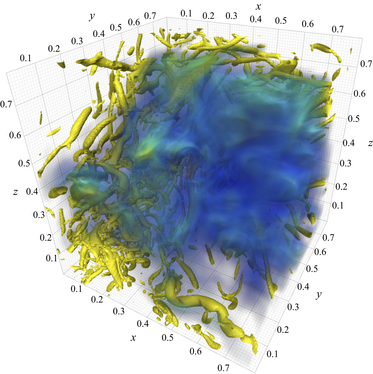Both $Q(\boldsymbol {x},t_0)$ and $e(\boldsymbol {x},t_0)$ are plotted in figure 4; the $Q$ distribution is shown as a $Q=500$ isosurface (yellow) displaying small-scale vortices in isotropic turbulence, while the energy is shown using volume rendering with transparency. Opening the figure at https://www.cambridge.org/S002211202200903X/figure-4/files/Figure4.html enables readers to rotate and zoom into the three-dimensional object, as well to change the $Q$ thresholds, transparency and colour parameters for the kinetic energy volume rendering. Such interactive manipulations can assist in improving the reader's understanding of the spatial distribution of the physical variables being plotted. Once again, the underlying data are provided as part of the notebook directory attached to the figure.

Figure 4. Iso-surface of $Q=500$ (yellow) and volume rendering of local kinetic energy in a small $128^3$ grid point subset of isotropic turbulence at $Re_\lambda = 430$. The overall domain of DNS is $[0,2\pi ]^3$. To view the interactive figure, go to https://www.cambridge.org/S002211202200903X/figure-4/files/Figure4.html. The directory including the data and the Jupyter notebook can be accessed at https://www.cambridge.org/S002211202200903X/figure-4.

Finally, we remark that notebooks can also be used to house animations, and it is likely that future developments of computational packages will open up many additional capabilities.

Authors submitting papers with accompanying computational notebooks (in Python, as a Jupyter notebook) will prepare a folder for each figure containing the notebook and accompanying data which will be associated with the submitted paper via a preliminary link. Referees will be asked and expected to examine the notebook to evaluate quality, functioning and value added to the paper. They will provide feedback to authors and revisions to the notebooks will be possible during review. Readers of accepted papers will be able to open the notebook by copying the entire directory to their own environment and clicking the Jupyter notebook file. They will then be able to view the published figure object and modify the notebook for their own usage (e.g. change parameters, etc.). Some interactive figure objects residing in the directory will be visible immediately via a direct link (such as the example in figure 4). Full details of how to prepare and submit a paper with Notebooks can be found here: https://www.cambridge.org/JFMNotebooks. As a new initiative the workflows around these submissions will evolve over time as we learn and we are looking forward to working with the community to develop JFM Notebooks into a valuable resource.

We very much look forward to receiving submissions that leverage the interactive capabilities of JFM Notebooks, starting now. JFM Notebooks can more fully convey the essence, complexity and beauty of fluid flow phenomena and, we hope, successfully scale up how individual fluid mechanics researchers communicate results to each other and to the wider community of JFM readers.