


1 Introduction
Buoyancy-driven, bidirectional flow in channels or tubes is relevant to many natural and industrial processes. Examples include lubricated pipelining that facilitates transport of viscous oil through pipelines by injecting lubricants like water (e.g. Joseph et al. Reference Joseph, Bai, Chen and Renardy1997), the flow of cement into drilling mud in wellbores (e.g. Frigaard & Scherzer Reference Frigaard and Scherzer1998), the counterflow of currents with different densities in oceanic straits (e.g. Dalziel Reference Dalziel1992) and magma circulation in the conduits of persistently degassing volcanoes (e.g. Stevenson & Blake Reference Stevenson and Blake1998).
The buoyancy-driven exchange flow between two immiscible fluids in a vertical tube is rarely if ever stable (e.g. Joseph et al. Reference Joseph, Bai, Chen and Renardy1997). Significant effort has been devoted to identifying the various pertinent flow types, including the formation of bubbles, slugs and side-by-side flow (e.g. Joseph & Renardy Reference Joseph and Renardy1992; Brauner Reference Brauner1998). Here, we investigate the flow variability associated with core–annular flow, the most commonly observed flow regime of exchange flows in vertical pipes. The core–annular geometry is characterized by one fluid flowing in the centre of the tube (core) surrounded by a film of the other fluid wetting the tube walls (annulus).
Numerous authors have examined the linear stability of core–annular flow (e.g. Joseph et al. Reference Joseph, Bai, Chen and Renardy1997). In the vertical configuration, Hickox (Reference Hickox1971) studied the linear stability of Poiseuille flow in the limit of long waves, assuming the fluid viscosity in the core is less than in the annulus. Despite the instability of the flow to long waves, a high viscosity contrast and surface tension notably suppress the growth rate of interface instabilities. Preziosi, Chen & Joseph (Reference Preziosi, Chen and Joseph1989) focused on the linear stability of the flow when the less viscous fluid occupies the annulus, Hu & Joseph (Reference Hu and Joseph1989) extended their analysis to different flow arrangements and Chen, Bai & Joseph (Reference Chen, Bai and Joseph1990) included the effects of gravity. Chen & Joseph (Reference Chen and Joseph1991) considered the nonlinear stability of core–annular flows. Bai, Chen & Joseph (Reference Bai, Chen and Joseph1992) compared the predictions of linear stability theory with experiments and documented new flow types characterized by nearly stationary interface waves, termed bamboo and corkscrew waves, that correspond approximately to the fastest-growing wavelength, suggesting that core–annular flow reaches a metastable flow configuration despite its inherent instability.
Our study seeks to explain the variability of core–annular flow between two Newtonian fluids in a vertical tube at low Reynolds number. Our work is motivated primarily by the need to better understand degassing processes in persistently active volcanoes, the most common form of volcanism on Earth. Many persistently degassing volcanoes have been active for periods exceeding the historical record. Although erupting comparatively small amounts of lava, they continuously emit copious amounts of volatiles and thermal energy, suggesting that the majority of magma is recycled back into the plumbing system after decoupling from the gas phase near the surface (e.g. Francis, Oppenheimer & Stevenson Reference Francis, Oppenheimer and Stevenson1993). At steady state, the ascent of gas-rich, buoyant magma in the conduit would therefore approximately balance the simultaneous descent of gas-poor, dense magma, which would result in exchange flow in the volcanic conduit (Kazahaya, Shinohara & Saito Reference Kazahaya, Shinohara and Saito1994; Stevenson & Blake Reference Stevenson and Blake1998; Burton, Mader & Polacci Reference Burton, Mader and Polacci2007; Witham Reference Witham2011).
The motivation to better understand volcanic degassing informs the parameter range we investigate in this paper. The density contrast between the two fluids is the consequence of gas bubbles exsolving from the magma. In the context of bidirectional flow, it is assumed that these gas bubbles are small compared to the radius of the conduit and remain entrained in the upwelling fluid. The resulting density difference tends to be much less variable than the viscosity ratio between the two fluids, which can vary by multiple orders of magnitude. For example, exsolution of 1 wt. % water typically increases the viscosity of the silicate melt by approximately a factor of 10 (e.g. McBirney & Murase Reference McBirney and Murase1984). Volatile loss also tends to be associated with crystallization, which can further significantly increase the effective viscosity of the degassed magma (e.g. McBirney & Murase Reference McBirney and Murase1984). Our main emphasis is hence on bidirectional flow with high viscosity contrast in vertical, or close to vertical, pipes, building on work by Joseph, Renardy & Renardy (Reference Joseph, Renardy and Renardy1984), but at very low Reynolds number.
In the volcanic context, the upwelling magma in the core is typically less viscous than the downwelling magma in the annulus, because it is more volatile rich. This arrangement is contrary to the typical arrangement in lubricated pipelining and tends to be unstable at finite Reynolds number, as demonstrated theoretically (Joseph et al. Reference Joseph, Renardy and Renardy1984) and experimentally (Arakeri et al. Reference Arakeri, Avila, Dada and Tovar2000; Huppert & Hallworth Reference Huppert and Hallworth2007). However, at the low Reynolds numbers and large viscosity contrasts likely representative of volcanic systems, core–annular flow with the less viscous fluid in the core becomes stable (Hickox Reference Hickox1971; Joseph et al. Reference Joseph, Renardy and Renardy1984; Stevenson & Blake Reference Stevenson and Blake1998).
Another important difference between bidirectional flow in volcanic systems and that in lubricated pipelining is the miscibility of the two fluids involved. Despite their different properties, the upwelling and downwelling magmas in volcanic conduits are miscible. The diffusivities of the magmas, however, are probably sufficiently low to mimic immiscible flows. Experimental studies have shown that miscible bidirectional flow at low diffusivity exhibits similar flow regimes as immiscible flow (Petitjeans & Maxworthy Reference Petitjeans and Maxworthy1996; Scoffoni, Lajeunesse & Homsy Reference Scoffoni, Lajeunesse and Homsy2001), including the characteristic corkscrew waves at the fluid interface observed in the immiscible context (e.g. Bai et al. Reference Bai, Chen and Joseph1992; Hu & Patankar Reference Hu and Patankar1995; Renardy Reference Renardy1997). Linear stability analysis, however, has suggested that even a small degree of mixing at the interface can stabilize the flow over a wide range of conditions (Vanaparthy, Meiburg & Wilhelm Reference Vanaparthy, Meiburg and Wilhelm2003; Meiburg et al. Reference Meiburg, Vanaparthy, Payr and Wilhelm2004).
Our work builds on laboratory experiments of exchange flow in closed vertical tubes conducted by Stevenson & Blake (Reference Stevenson and Blake1998) and Beckett et al. (Reference Beckett, Mader, Phillips, Rust and Witham2011). We focus on this specific set of experiments because the parameter range is representative of volcanic systems. We analyse the flow behaviour observed in the laboratory by using direct numerical simulations to virtually reproduce the original experiments. Our numerical model does not require closures such as drag forces, interface stresses or rise speeds (Suckale et al. Reference Suckale, Hager, Elkins-Tanton and Nave2010a ; Suckale, Nave & Hager Reference Suckale, Nave and Hager2010b ; Qin & Suckale Reference Qin and Suckale2017). Instead, these flow properties emerge self-consistently from the computation, as in analogue experiments where the flow dynamics emerges directly from the experimental set-up and the materials used. Direct numerical simulations hence enable us to quantify velocities, stresses, and other flow variables at all times and locations in the flow field and to extend experiments to scales or flow conditions not realizable in a laboratory setting.
We link our direct numerical simulations to an analytical model of laminar core–annular flow in a vertical tube at steady state, building on previous similar approaches (e.g. Russell & Charles Reference Russell and Charles1959; Kazahaya et al. Reference Kazahaya, Shinohara and Saito1994; Ullmann & Brauner Reference Ullmann and Brauner2004; Huppert & Hallworth Reference Huppert and Hallworth2007). We predict the existence of two distinct solutions at steady-state conditions: a solution with fast flow in a thin core and a solution with relatively slow flow in a thick core. The existence of two solutions suggests that exchange flow in vertical tubes is a bistable problem. We test this hypothesis through direct numerical simulations (§ 2.2) and find that the boundary conditions control which solution is realized in a laboratory experiment (§ 3). This insight implies that the bidirectional flow regime in vertical tubes cannot be predicted based on geometry and material parameters alone – an aspect of core–annular flow that could have important implications for understanding the variability of magma circulation in volcanic conduits and the resulting eruptive activity (§ 4).
2 Model description
We combine two distinct and complementary model components: an analytical model of core–annular flow at steady state, and direct numerical simulations of exchange flow in two dimensions. We focus on two-dimensional (2-D) numerical simulations to afford higher resolution of the evolving interface. Whereas the analytical model is limited to core–annular flow of immiscible fluids, our numerical approach can capture the various flow regimes that arise for both the miscible fluids employed in the laboratory experiments and the immiscible fluids assumed in the analytical model.
Sketch of the core–annular geometry and key variables used for a vertical (a) and a horizontal (b) cross-section. The interface between the two fluids is depicted as wavy to highlight the unstable nature of the flow pattern.
2.1 Analytical model
2.1.1 Derivation
At low Reynolds number, the steady-state core–annular flow of two immiscible and incompressible Newtonian fluids in a pipe of inclination
 $\unicode[STIX]{x1D6FC}$
from the vertical direction can be described by the 1-D Stokes equations along the radial coordinate
$\unicode[STIX]{x1D6FC}$
from the vertical direction can be described by the 1-D Stokes equations along the radial coordinate
 $r\in [0,R]$
(see figure 1),
$r\in [0,R]$
(see figure 1),
 $$\begin{eqnarray}\displaystyle \unicode[STIX]{x1D707}_{d}\frac{1}{r}\frac{\text{d}}{\text{d}r}\left(r\frac{\text{d}u_{d}}{\text{d}r}\right) & = & \displaystyle \frac{\text{d}p}{\text{d}z}+\unicode[STIX]{x1D70C}_{d}g\cos \unicode[STIX]{x1D6FC},\quad r\in [\unicode[STIX]{x1D6FF},R],\end{eqnarray}$$
 $$\begin{eqnarray}\displaystyle \unicode[STIX]{x1D707}_{a}\frac{1}{r}\frac{\text{d}}{\text{d}r}\left(r\frac{\text{d}u_{a}}{\text{d}r}\right) & = & \displaystyle \frac{\text{d}p}{\text{d}z}+\unicode[STIX]{x1D70C}_{a}g\cos \unicode[STIX]{x1D6FC},\quad r\in [0,\unicode[STIX]{x1D6FF}],\end{eqnarray}$$
 $(\cdot )_{d}$
and
$(\cdot )_{d}$
and
 $(\cdot )_{a}$
denote the descending and ascending fluid properties, namely dynamic viscosity
$(\cdot )_{a}$
denote the descending and ascending fluid properties, namely dynamic viscosity
 $\unicode[STIX]{x1D707}$
, density
$\unicode[STIX]{x1D707}$
, density
 $\unicode[STIX]{x1D70C}$
and vertical speed
$\unicode[STIX]{x1D70C}$
and vertical speed
 $u$
, respectively,
$u$
, respectively,
 $R$
is the pipe radius,
$R$
is the pipe radius,
 $g$
the gravitational acceleration and
$g$
the gravitational acceleration and
 $\unicode[STIX]{x1D6FF}$
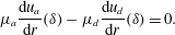
represents the unknown location of the interface between the ascending and descending fluids. The pressure drop is an unknown constant to be determined. The boundary conditions are no-slip at the tube wall,
$\unicode[STIX]{x1D6FF}$
represents the unknown location of the interface between the ascending and descending fluids. The pressure drop is an unknown constant to be determined. The boundary conditions are no-slip at the tube wall,  $$\begin{eqnarray}\displaystyle u_{d}(R)=0, & & \displaystyle\end{eqnarray}$$
vanishing radial stress at the symmetry line in the tube centre,
 $$\begin{eqnarray}\displaystyle \frac{\text{d}u_{a}}{\text{d}r}(0)=0, & & \displaystyle\end{eqnarray}$$
and continuity of velocity and shear stress across the fluid–fluid interface,
 $$\begin{eqnarray}\displaystyle & \displaystyle u_{d}(\unicode[STIX]{x1D6FF})-u_{a}(\unicode[STIX]{x1D6FF})=0, & \displaystyle\end{eqnarray}$$
 $$\begin{eqnarray}\displaystyle & \displaystyle \unicode[STIX]{x1D707}_{a}\frac{\text{d}u_{a}}{\text{d}r}(\unicode[STIX]{x1D6FF})-\unicode[STIX]{x1D707}_{d}\frac{\text{d}u_{d}}{\text{d}r}(\unicode[STIX]{x1D6FF})=0. & \displaystyle\end{eqnarray}$$
Instead of a phase flow-rate scaling (Ullmann & Brauner Reference Ullmann and Brauner2004), we define the non-dimensional quantities
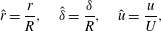 $$\begin{eqnarray}\displaystyle \hat{r}={\displaystyle \frac{r}{R}},\quad \hat{\unicode[STIX]{x1D6FF}}={\displaystyle \frac{\unicode[STIX]{x1D6FF}}{R}},\quad \hat{u} ={\displaystyle \frac{u}{U}}, & & \displaystyle\end{eqnarray}$$
where we define
 $U=\unicode[STIX]{x0394}\unicode[STIX]{x1D70C}gR^{2}/\unicode[STIX]{x1D707}_{d}$
, the viscous rise speed due to the density difference
$U=\unicode[STIX]{x0394}\unicode[STIX]{x1D70C}gR^{2}/\unicode[STIX]{x1D707}_{d}$
, the viscous rise speed due to the density difference
 $\unicode[STIX]{x0394}\unicode[STIX]{x1D70C}=\unicode[STIX]{x1D70C}_{d}-\unicode[STIX]{x1D70C}_{a}$
. Substituting (2.6) into (2.1) and dropping all hats yields the dimensionless equations,
$\unicode[STIX]{x0394}\unicode[STIX]{x1D70C}=\unicode[STIX]{x1D70C}_{d}-\unicode[STIX]{x1D70C}_{a}$
. Substituting (2.6) into (2.1) and dropping all hats yields the dimensionless equations,
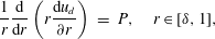 $$\begin{eqnarray}\displaystyle \frac{1}{r}\frac{\text{d}}{\text{d}r}\left(r\frac{\text{d}u_{d}}{\unicode[STIX]{x2202}r}\right) & = & \displaystyle P,\quad r\in [\unicode[STIX]{x1D6FF},1],\end{eqnarray}$$
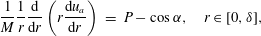 $$\begin{eqnarray}\displaystyle \frac{1}{M}\frac{1}{r}\frac{\text{d}}{\text{d}r}\left(r\frac{\text{d}u_{a}}{\text{d}r}\right) & = & \displaystyle P-\cos \unicode[STIX]{x1D6FC},\quad r\in [0,\unicode[STIX]{x1D6FF}],\end{eqnarray}$$
 $P=(\text{d}p/\text{d}z+\unicode[STIX]{x1D70C}_{d}g\,\text{cos}\,\unicode[STIX]{x1D6FC})/(g\unicode[STIX]{x0394}\unicode[STIX]{x1D70C})$
is the non-dimensional pressure drop and
$P=(\text{d}p/\text{d}z+\unicode[STIX]{x1D70C}_{d}g\,\text{cos}\,\unicode[STIX]{x1D6FC})/(g\unicode[STIX]{x0394}\unicode[STIX]{x1D70C})$
is the non-dimensional pressure drop and
 $M=\unicode[STIX]{x1D707}_{d}/\unicode[STIX]{x1D707}_{a}$
is the viscosity ratio. We integrate equations (2.7), while accounting for appropriately non-dimensionalized boundary conditions, to obtain
$M=\unicode[STIX]{x1D707}_{d}/\unicode[STIX]{x1D707}_{a}$
is the viscosity ratio. We integrate equations (2.7), while accounting for appropriately non-dimensionalized boundary conditions, to obtain  $$\begin{eqnarray}\displaystyle u_{d}(r) & = & \displaystyle \frac{P}{4}(r^{2}-1)-\frac{\unicode[STIX]{x1D6FF}^{2}}{2}\cos \unicode[STIX]{x1D6FC}\log r,\quad r\in [\unicode[STIX]{x1D6FF},1],\end{eqnarray}$$
 $$\begin{eqnarray}\displaystyle u_{a}(r) & = & \displaystyle M\frac{P-\cos \unicode[STIX]{x1D6FC}}{4}(r^{2}-\unicode[STIX]{x1D6FF}^{2})+u_{i},\quad r\in [0,\unicode[STIX]{x1D6FF}],\end{eqnarray}$$
 $u_{i}=u_{d}(\unicode[STIX]{x1D6FF})=u_{a}(\unicode[STIX]{x1D6FF})$
is the vertical flow speed at the interface given by
$u_{i}=u_{d}(\unicode[STIX]{x1D6FF})=u_{a}(\unicode[STIX]{x1D6FF})$
is the vertical flow speed at the interface given by  $$\begin{eqnarray}\displaystyle u_{i}=\frac{P}{4}(\unicode[STIX]{x1D6FF}^{2}-1)-\frac{\unicode[STIX]{x1D6FF}^{2}}{2}\cos \unicode[STIX]{x1D6FC}\log \unicode[STIX]{x1D6FF}. & & \displaystyle\end{eqnarray}$$
The ascending flux in a closed tube with incompressible fluids must exactly balance the descending flux,
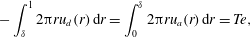 $$\begin{eqnarray}\displaystyle -\int _{\unicode[STIX]{x1D6FF}}^{1}2\unicode[STIX]{x03C0}ru_{d}(r)\,\text{d}r=\int _{0}^{\unicode[STIX]{x1D6FF}}2\unicode[STIX]{x03C0}ru_{a}(r)\,\text{d}r=Te, & & \displaystyle\end{eqnarray}$$
where
 $Te$
is the dimensionless flux or Transport number (e.g. Huppert & Hallworth Reference Huppert and Hallworth2007). The Transport number is related, but not identical, to the Poiseuille number,
$Te$
is the dimensionless flux or Transport number (e.g. Huppert & Hallworth Reference Huppert and Hallworth2007). The Transport number is related, but not identical, to the Poiseuille number,
 $Ps$
, defined in Stevenson & Blake (Reference Stevenson and Blake1998),
$Ps$
, defined in Stevenson & Blake (Reference Stevenson and Blake1998),
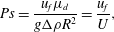 $$\begin{eqnarray}\displaystyle Ps=\frac{u_{f}\unicode[STIX]{x1D707}_{d}}{g\unicode[STIX]{x0394}\unicode[STIX]{x1D70C}R^{2}}=\frac{u_{f}}{U}, & & \displaystyle\end{eqnarray}$$
where
 $u_{f}$
is the (dimensional) terminal rise speed of the ascending front (see the supplementary material available at https://doi.org/10.1017/jfm.2018.382 for details). The
$u_{f}$
is the (dimensional) terminal rise speed of the ascending front (see the supplementary material available at https://doi.org/10.1017/jfm.2018.382 for details). The
 $Ps$
number therefore represents the non-dimensional rise speed, whereas the
$Ps$
number therefore represents the non-dimensional rise speed, whereas the
 $Te$
number captures the non-dimensional flux, and hence
$Te$
number captures the non-dimensional flux, and hence
 $$\begin{eqnarray}\displaystyle Te=\frac{Ps}{\unicode[STIX]{x03C0}\unicode[STIX]{x1D6FF}^{2}}. & & \displaystyle\end{eqnarray}$$
We focus on
 $Te$
in our analysis, because the flux is balanced between ascending and descending fluids and does not hinge on selecting either a characteristic rise speed from the spatially variable function,
$Te$
in our analysis, because the flux is balanced between ascending and descending fluids and does not hinge on selecting either a characteristic rise speed from the spatially variable function,
 $u_{a}(r)$
, or a core radius,
$u_{a}(r)$
, or a core radius,
 $\unicode[STIX]{x1D6FF}$
. To fulfil the constraint of no net flux in the tube, we substitute (2.8) into (2.10) and solve for the driving force
$\unicode[STIX]{x1D6FF}$
. To fulfil the constraint of no net flux in the tube, we substitute (2.8) into (2.10) and solve for the driving force
 $P$
, which depends only on the dimensionless parameters of the problem (i.e.
$P$
, which depends only on the dimensionless parameters of the problem (i.e.
 $\unicode[STIX]{x1D6FF}$
,
$\unicode[STIX]{x1D6FF}$
,
 $M$
,
$M$
,
 $\unicode[STIX]{x1D6FC}$
):
$\unicode[STIX]{x1D6FC}$
):
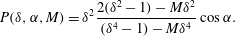 $$\begin{eqnarray}\displaystyle P(\unicode[STIX]{x1D6FF},\unicode[STIX]{x1D6FC},M)=\unicode[STIX]{x1D6FF}^{2}\frac{2(\unicode[STIX]{x1D6FF}^{2}-1)-M\unicode[STIX]{x1D6FF}^{2}}{(\unicode[STIX]{x1D6FF}^{4}-1)-M\unicode[STIX]{x1D6FF}^{4}}\cos \unicode[STIX]{x1D6FC}. & & \displaystyle\end{eqnarray}$$
We can now express
 $Te$
as a function of
$Te$
as a function of
 $P$
and
$P$
and
 $\unicode[STIX]{x1D6FF}$
:
$\unicode[STIX]{x1D6FF}$
:
 $$\begin{eqnarray}\displaystyle Te(\unicode[STIX]{x1D6FF},\unicode[STIX]{x1D6FC},M)=2\unicode[STIX]{x03C0}\left[\frac{P}{16}(\unicode[STIX]{x1D6FF}^{2}-1)^{2}+\frac{\unicode[STIX]{x1D6FF}^{2}}{8}\cos \unicode[STIX]{x1D6FC}(\unicode[STIX]{x1D6FF}^{2}-1-2\unicode[STIX]{x1D6FF}^{2}\log \unicode[STIX]{x1D6FF})\right]. & & \displaystyle\end{eqnarray}$$
We note that once
 $P$
and
$P$
and
 $\unicode[STIX]{x1D6FF}$
are defined,
$\unicode[STIX]{x1D6FF}$
are defined,
 $Te$
is uniquely specified. The opposite, however, is not true. The quadratic and quartic terms in (2.14) suggest that a given flux,
$Te$
is uniquely specified. The opposite, however, is not true. The quadratic and quartic terms in (2.14) suggest that a given flux,
 $Te$
, could be achieved for two different
$Te$
, could be achieved for two different
 $\unicode[STIX]{x1D6FF}$
. Even though the model developed by Huppert & Hallworth (Reference Huppert and Hallworth2007) also admits multiple solutions, the authors implicitly imposed uniqueness by maximizing the flux or, alternatively, extremizing the dissipation in the system. In § 3, we numerically explore the validity of this uniqueness hypothesis, characterize the differences between the two possible solutions in more detail, and investigate whether both solutions are relevant in practice.
$\unicode[STIX]{x1D6FF}$
. Even though the model developed by Huppert & Hallworth (Reference Huppert and Hallworth2007) also admits multiple solutions, the authors implicitly imposed uniqueness by maximizing the flux or, alternatively, extremizing the dissipation in the system. In § 3, we numerically explore the validity of this uniqueness hypothesis, characterize the differences between the two possible solutions in more detail, and investigate whether both solutions are relevant in practice.
2.2 Numerical model
2.2.1 Governing equations
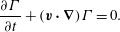
Our numerical model solves for conservation of mass and momentum. We assume that both fluids are incompressible. The governing equations are hence the incompressibility condition,
 $$\begin{eqnarray}\displaystyle \unicode[STIX]{x1D735}\boldsymbol{\cdot }\boldsymbol{v}=0, & & \displaystyle\end{eqnarray}$$
and the variable-coefficient Navier–Stokes equation,
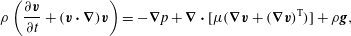 $$\begin{eqnarray}\displaystyle \unicode[STIX]{x1D70C}\left(\frac{\unicode[STIX]{x2202}\boldsymbol{v}}{\unicode[STIX]{x2202}t}+(\boldsymbol{v}\boldsymbol{\cdot }\unicode[STIX]{x1D735})\boldsymbol{v}\right)=-\unicode[STIX]{x1D735}p+\unicode[STIX]{x1D735}\boldsymbol{\cdot }[\unicode[STIX]{x1D707}(\unicode[STIX]{x1D735}\boldsymbol{v}+(\unicode[STIX]{x1D735}\boldsymbol{v})^{\text{T}})]+\unicode[STIX]{x1D70C}\boldsymbol{g}, & & \displaystyle\end{eqnarray}$$
where
 $\boldsymbol{v}$
is the velocity, and
$\boldsymbol{v}$
is the velocity, and
 $p$
the pressure.
$p$
the pressure.
Density and viscosity vary in space and time to reflect the different properties of the two fluids. We consider the two contrasting scenarios of immiscible and miscible fluids. The immiscible case is useful for a direct comparison with the analytical solution, which is strictly valid only for two immiscible fluids. The miscible case represents the experimental set-up of Stevenson & Blake (Reference Stevenson and Blake1998), which involves two miscible fluids with low diffusivity.
2.2.2 Immiscible fluids
In the immiscible case, a sharp interface separates the two fluids. We advect the curve,
 $\unicode[STIX]{x1D6E4}$
, which represents this interface, with the flow field according to
$\unicode[STIX]{x1D6E4}$
, which represents this interface, with the flow field according to
 $$\begin{eqnarray}\displaystyle \frac{\unicode[STIX]{x2202}\unicode[STIX]{x1D6E4}}{\unicode[STIX]{x2202}t}+(\boldsymbol{v}\boldsymbol{\cdot }\unicode[STIX]{x1D735})\unicode[STIX]{x1D6E4}=0. & & \displaystyle\end{eqnarray}$$
The interface deforms in response to the hydrodynamic forces acting on it. The material properties change discontinuously at the interface:
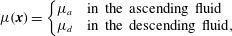 $$\begin{eqnarray}\displaystyle \unicode[STIX]{x1D707}(\boldsymbol{x})=\left\{\begin{array}{@{}ll@{}}\unicode[STIX]{x1D707}_{a} & \text{in the ascending fluid}\\ \unicode[STIX]{x1D707}_{d} & \text{in the descending fluid},\end{array}\right. & & \displaystyle\end{eqnarray}$$
and
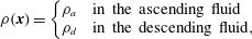 $$\begin{eqnarray}\displaystyle \unicode[STIX]{x1D70C}(\boldsymbol{x})=\left\{\begin{array}{@{}rl@{}}\unicode[STIX]{x1D70C}_{a} & \text{in the ascending fluid}\\ \unicode[STIX]{x1D70C}_{d} & \text{in the descending fluid},\end{array}\right. & & \displaystyle\end{eqnarray}$$
and may entail a jump in the pressure and normal stresses at the interface:
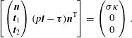 $$\begin{eqnarray}\displaystyle \left[\left(\begin{array}{@{}c@{}}\boldsymbol{n}\\ \boldsymbol{t}_{1}\\ \boldsymbol{t}_{2}\end{array}\right)(p\unicode[STIX]{x1D644}-\unicode[STIX]{x1D749})\boldsymbol{n}^{\text{T}}\right]=\left(\begin{array}{@{}c@{}}\unicode[STIX]{x1D70E}\unicode[STIX]{x1D705}\\ 0\\ 0\end{array}\right). & & \displaystyle\end{eqnarray}$$
Square brackets
 $[\cdot ]$
denote a jump at the fluid–fluid interface,
$[\cdot ]$
denote a jump at the fluid–fluid interface,
 $\unicode[STIX]{x1D644}$
is the identity tensor,
$\unicode[STIX]{x1D644}$
is the identity tensor,
 $\unicode[STIX]{x1D749}=\unicode[STIX]{x1D707}(\unicode[STIX]{x1D735}\boldsymbol{v}+(\unicode[STIX]{x1D735}\boldsymbol{v})^{\text{T}})$
the viscous stress tensor,
$\unicode[STIX]{x1D749}=\unicode[STIX]{x1D707}(\unicode[STIX]{x1D735}\boldsymbol{v}+(\unicode[STIX]{x1D735}\boldsymbol{v})^{\text{T}})$
the viscous stress tensor,
 $\unicode[STIX]{x1D70E}$
the surface tension,
$\unicode[STIX]{x1D70E}$
the surface tension,
 $\unicode[STIX]{x1D705}$
the curvature of
$\unicode[STIX]{x1D705}$
the curvature of
 $\unicode[STIX]{x1D6E4}$
,
$\unicode[STIX]{x1D6E4}$
,
 $\boldsymbol{n}$
the unit normal vector on
$\boldsymbol{n}$
the unit normal vector on
 $\unicode[STIX]{x1D6E4}$
pointing from the ascending towards the descending fluid and
$\unicode[STIX]{x1D6E4}$
pointing from the ascending towards the descending fluid and
 $\boldsymbol{t}_{1}$
and
$\boldsymbol{t}_{1}$
and
 $\boldsymbol{t}_{2}$
the two unit tangential vectors on
$\boldsymbol{t}_{2}$
the two unit tangential vectors on
 $\unicode[STIX]{x1D6E4}$
. Solving the Navier–Stokes equation and introducing surface tensions implies that additional non-dimensional numbers are needed to describe the flow behaviour. We choose the Reynolds number,
$\unicode[STIX]{x1D6E4}$
. Solving the Navier–Stokes equation and introducing surface tensions implies that additional non-dimensional numbers are needed to describe the flow behaviour. We choose the Reynolds number,
 $Re=\unicode[STIX]{x0394}\unicode[STIX]{x1D70C}UR/\unicode[STIX]{x1D707}_{d}$
, the Bond number,
$Re=\unicode[STIX]{x0394}\unicode[STIX]{x1D70C}UR/\unicode[STIX]{x1D707}_{d}$
, the Bond number,
 $Bo=\unicode[STIX]{x0394}\unicode[STIX]{x1D70C}gR^{2}/\unicode[STIX]{x1D70E}$
and the Froude number,
$Bo=\unicode[STIX]{x0394}\unicode[STIX]{x1D70C}gR^{2}/\unicode[STIX]{x1D70E}$
and the Froude number,
 $Fr=U^{2}/(gR)$
(see the supplementary material for a summary table). All the immiscible simulations shown in the manuscript represent the case of no surface tension,
$Fr=U^{2}/(gR)$
(see the supplementary material for a summary table). All the immiscible simulations shown in the manuscript represent the case of no surface tension,
 $\unicode[STIX]{x1D70E}=0$
, but we discuss the effect of surface tension on interface instabilities briefly in the supplementary material.
$\unicode[STIX]{x1D70E}=0$
, but we discuss the effect of surface tension on interface instabilities briefly in the supplementary material.
2.2.3 Miscible fluids
To allow for mixing, we introduce a continuous variable,
 $c$
, which represents the concentration of the buoyant fluid. Initially, the concentration is set to unity in the buoyant fluid and zero in the heavy fluid. The concentration evolves over time due to advection and diffusion,
$c$
, which represents the concentration of the buoyant fluid. Initially, the concentration is set to unity in the buoyant fluid and zero in the heavy fluid. The concentration evolves over time due to advection and diffusion,
 $$\begin{eqnarray}\displaystyle \frac{\unicode[STIX]{x2202}c}{\unicode[STIX]{x2202}t}+\boldsymbol{v}\boldsymbol{\cdot }\unicode[STIX]{x1D735}c=D\unicode[STIX]{x1D6FB}^{2}c, & & \displaystyle\end{eqnarray}$$
where
 $D$
is the diffusion coefficient. In their experiments, Stevenson & Blake (Reference Stevenson and Blake1998) used miscible fluids, such as syrup, dilute syrup, glycerol and water, but did not report the fluid diffusivities. In the absence of detailed measurements, we use a constant diffusivity of
$D$
is the diffusion coefficient. In their experiments, Stevenson & Blake (Reference Stevenson and Blake1998) used miscible fluids, such as syrup, dilute syrup, glycerol and water, but did not report the fluid diffusivities. In the absence of detailed measurements, we use a constant diffusivity of
 $D=10^{-10}~\text{m}^{2}~\text{s}^{-1}$
in both fluids for all simulations, a value motivated by the diffusivity measured for corn syrup in distilled water (Ray, Bunton & Pojman Reference Ray, Bunton and Pojman2007). Miscibility adds another non-dimensional parameter, the Péclet number, which quantifies the relative importance of advection to diffusion
$D=10^{-10}~\text{m}^{2}~\text{s}^{-1}$
in both fluids for all simulations, a value motivated by the diffusivity measured for corn syrup in distilled water (Ray, Bunton & Pojman Reference Ray, Bunton and Pojman2007). Miscibility adds another non-dimensional parameter, the Péclet number, which quantifies the relative importance of advection to diffusion
 $Pe=RU/D$
.
$Pe=RU/D$
.
We assume that density and viscosity depend linearly on the concentration
 $c$
, such that
$c$
, such that
 $$\begin{eqnarray}\displaystyle \unicode[STIX]{x1D70C}=\unicode[STIX]{x1D70C}_{d}+c(\unicode[STIX]{x1D70C}_{a}-\unicode[STIX]{x1D70C}_{d}) & & \displaystyle\end{eqnarray}$$
and
 $$\begin{eqnarray}\displaystyle \unicode[STIX]{x1D707}=\unicode[STIX]{x1D707}_{d}+c(\unicode[STIX]{x1D707}_{a}-\unicode[STIX]{x1D707}_{d}). & & \displaystyle\end{eqnarray}$$
We note that additional complexity may arise in the vicinity of the interface if a nonlinear dependence of viscosity on concentration is assumed (see the supplementary material for details), as is the case in some prior studies (e.g. Tan & Homsy Reference Tan and Homsy1986; Goyal & Meiburg Reference Goyal and Meiburg2006).
To initialize the miscible simulations, we assume that the initial concentration field has an interface with a finite thickness of
 $1.5\unicode[STIX]{x0394}x$
, where
$1.5\unicode[STIX]{x0394}x$
, where
 $\unicode[STIX]{x0394}x$
is the coarse grid resolution (see § 2.2.4 and figure 2). Hence, no discontinuous material contrasts arise in our miscible computations.
$\unicode[STIX]{x0394}x$
is the coarse grid resolution (see § 2.2.4 and figure 2). Hence, no discontinuous material contrasts arise in our miscible computations.
Illustration of the initial conditions, boundary conditions and adaptive grid refinement for both immiscible and miscible flow. The grid is intentionally coarse for visualization purposes. (a,b) show immiscible fluids; (c,d) show miscible fluids.
2.2.4 Numerical methods
We discretize the governing equations, (2.15) and (2.16), on a Cartesian grid (see figure 2) using the numerical method derived, verified and validated in Qin & Suckale (Reference Qin and Suckale2017). For our computations, we opt for a Cartesian set-up rather than an axisymmetric formulation, because not all of the laboratory experiments we reproduce exhibit an axisymmetric symmetry and because of the importance of non-axisymmetric instabilities in core–annular flows (e.g. Hu & Patankar Reference Hu and Patankar1995; Renardy Reference Renardy1997).
Our numerical method was developed specifically for multiphase flow problems with large viscosity contrasts at low Reynolds number (Suckale et al. Reference Suckale, Nave and Hager2010b , Reference Suckale, Sethian, Yu and Elkins-Tanton2012). It consists of three main components. The first is a multiphase Navier–Stokes solver that handles substantial and discontinuous differences in the properties of material phases by adopting an implicit implementation of the viscous term, time-step splitting, and an approximate factorization of the sparse coefficient matrices for computational efficiency. The second component is a level-set-based interface solver that tracks the motion of a fluid–fluid interface through an iterative topology-preserving projection (Qin et al. Reference Qin, Delaney, Riaz and Balaras2015). The sharp interface solver is pertinent only if the two fluids are immiscible. In the computationally simpler case of two miscible fluids, we solve an advection–diffusion equation for concentration.
The third component is an adaptive grid refinement algorithm that increases resolution in the vicinity of the moving interface, where most of the salient physical processes originate. Accurate interface advection is highly dependent on grid resolution (e.g. Sethian Reference Sethian1996), particularly in flows that hinge sensitively on the growth of interface instabilities. To maximize numerical resolution at the interface, we adopt an adaptive mesh refinement strategy that tracks the interface position over time. Figure 2 shows a close up of the computational domain around the interface to schematically illustrate the grid refinement at the initial condition (figure 2 a) and at a later time (figure 2 b), both shown at intentionally coarse resolution for easier visualization. The refined zone extends as the interface is stretched by flow. Although the computational challenges associated with tracking a diffusive interface are less pronounced, we adopt the same grid refinement strategy for the miscible case (figure 2 c,d). For more details regarding the numerical technique, including the various benchmarks performed to verify and validate the numerical method, please refer to Qin & Suckale (Reference Qin and Suckale2017) and this study’s supplementary material.
3 Results
Direct numerical simulations afford the possibility to study flow behaviour beyond the scales, boundary conditions and material properties realizable in a laboratory setting. To generalize the scientific insights drawn from the laboratory work by Stevenson & Blake (Reference Stevenson and Blake1998), we start by reproducing the original experiments, proceed to a detailed analysis of the observed flow behaviour and then generalize the experiments by allowing for flow in and out of the tubes.
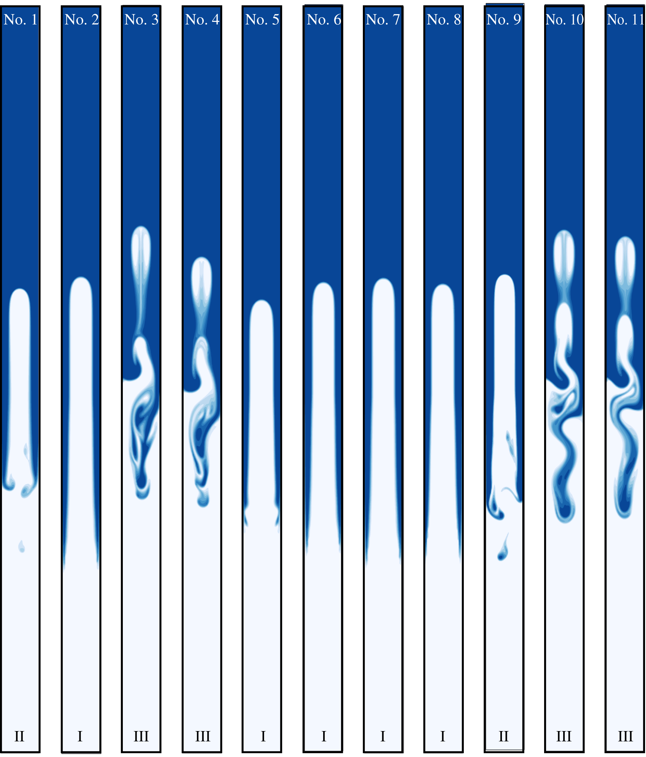
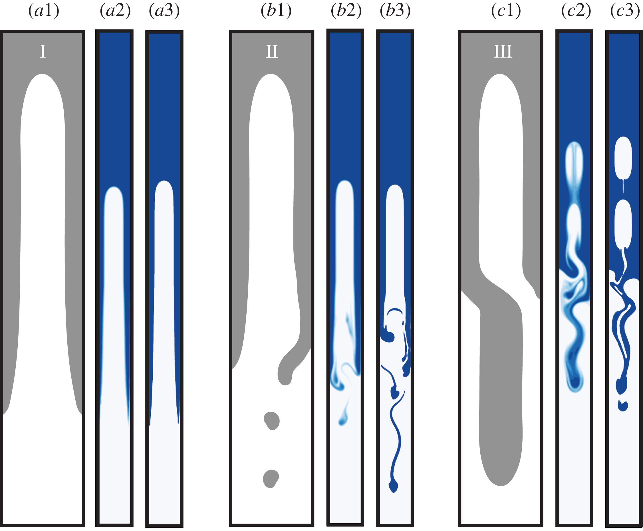
Numerical reproduction of all 11 experiments performed by Stevenson & Blake (Reference Stevenson and Blake1998) using two miscible fluids. The dense and the buoyant fluids are shown in dark and light blue, respectively. The aspect ratio of all laboratory tubes was
 $1:100$
despite different physical lengths and widths. Here and below, only the central part of the numerical domain is shown for better visibility. All simulations are shown at
$1:100$
despite different physical lengths and widths. Here and below, only the central part of the numerical domain is shown for better visibility. All simulations are shown at
 $t=200\times t_{0}$
, where
$t=200\times t_{0}$
, where
 $t_{0}=R/U$
is the non-dimensional time.
$t_{0}=R/U$
is the non-dimensional time.
3.1 Virtual reproductions of analogue experiments
Stevenson & Blake (Reference Stevenson and Blake1998) initiated their experiments by inverting closed tubes filled with the denser, more viscous fluid in the lower half, and the buoyant, less viscous fluid in the upper half. We start our simulations after the inversion step, such that the two fluids are unstably stratified with a slight cosine perturbation along their interface (see figure 2). We have verified that an initial condition of different symmetry yields qualitatively equivalent model outcomes, as shown in the supplementary material. To represent the rigid glass walls of the experimental test tubes, we set all four side boundaries to no slip (
 $\boldsymbol{v}=0$
). All simulations are computed on a
$\boldsymbol{v}=0$
). All simulations are computed on a
 $40\times 4000$
grid with a fourfold refinement at the interface. At this resolution, the flow dynamics is well resolved, as demonstrated by a convergence test included in the supplementary material.
$40\times 4000$
grid with a fourfold refinement at the interface. At this resolution, the flow dynamics is well resolved, as demonstrated by a convergence test included in the supplementary material.
We numerically reproduce all 11 analogue experiments performed by Stevenson & Blake (Reference Stevenson and Blake1998), based on the detailed material properties they reported (see table 1). All computations are performed for two miscible fluids with low diffusivity (i.e.
 $D=10^{-10}~\text{m}^{2}~\text{s}^{-1}$
). Figure 3 shows the fully developed flows at
$D=10^{-10}~\text{m}^{2}~\text{s}^{-1}$
). Figure 3 shows the fully developed flows at
 $t=200\times t_{0}$
, where
$t=200\times t_{0}$
, where
 $t_{0}=R/U$
is the dimensionless, viscous time scale.
$t_{0}=R/U$
is the dimensionless, viscous time scale.
We generally observe the same behaviour as reported by Stevenson & Blake (Reference Stevenson and Blake1998), which they classified into three different overturn styles. In figure 4, we illustrate these three overturn styles in the reproduced experiments No. 8, No. 9 and No. 10. At high viscosity ratios (
 $M>300$
), the flow configuration is characterized by stable core–annular flow (flow regime I; figure 4
a1–3). With decreasing viscosity contrast, interface waves become more pronounced. However, at intermediate viscosity ratios (
$M>300$
), the flow configuration is characterized by stable core–annular flow (flow regime I; figure 4
a1–3). With decreasing viscosity contrast, interface waves become more pronounced. However, at intermediate viscosity ratios (
 $10<M<300$
), the amplitude of interface waves remains small enough to avoid wave bridging and disintegration of the core (flow regime II; figure 4
b1–3). Rather, the descending fluid intermittently rips off the tube wall, while the ascending fluid forms a coherent core in the centre of the tube. Once the viscosity contrast becomes small (
$10<M<300$
), the amplitude of interface waves remains small enough to avoid wave bridging and disintegration of the core (flow regime II; figure 4
b1–3). Rather, the descending fluid intermittently rips off the tube wall, while the ascending fluid forms a coherent core in the centre of the tube. Once the viscosity contrast becomes small (
 $M<10$
), wave bridging occurs, and as a consequence, both fluids sink or rise as separate batches in the centre of the tube (flow regime III; figure 4
c1–3). We note that all three flow regimes exhibit interface waves. In agreement with the theory outlined by Hickox (Reference Hickox1971), the amplitude and dynamic significance of these interface waves decrease as the viscosity contrast increases.
$M<10$
), wave bridging occurs, and as a consequence, both fluids sink or rise as separate batches in the centre of the tube (flow regime III; figure 4
c1–3). We note that all three flow regimes exhibit interface waves. In agreement with the theory outlined by Hickox (Reference Hickox1971), the amplitude and dynamic significance of these interface waves decrease as the viscosity contrast increases.
Summary of analogue experimental data, and numerical and analytical results. Viscosity ratio (
 $M$
), density contrast (
$M$
), density contrast (
 $\unicode[STIX]{x0394}\unicode[STIX]{x1D70C}$
), tube radius (
$\unicode[STIX]{x0394}\unicode[STIX]{x1D70C}$
), tube radius (
 $R$
), tube length (
$R$
), tube length (
 $L$
), front rise speed (
$L$
), front rise speed (
 $u$
), Poiseuille number (
$u$
), Poiseuille number (
 $Ps$
), dimensionless core radius (
$Ps$
), dimensionless core radius (
 $\unicode[STIX]{x1D6FF}$
), and flow regime (Reg) observed in experiments (EXP) and numerical models (NUM). Thin-core,
$\unicode[STIX]{x1D6FF}$
), and flow regime (Reg) observed in experiments (EXP) and numerical models (NUM). Thin-core,
 $\unicode[STIX]{x1D6FF}_{thin}$
, and thick-core,
$\unicode[STIX]{x1D6FF}_{thin}$
, and thick-core,
 $\unicode[STIX]{x1D6FF}_{thick}$
, radii, and flow-reversal flux ratio
$\unicode[STIX]{x1D6FF}_{thick}$
, radii, and flow-reversal flux ratio
 $Te_{rev}/Te$
in analytical models (ANA). Bold numbers indicate the solution observed in corresponding experiments and simulations.
$Te_{rev}/Te$
in analytical models (ANA). Bold numbers indicate the solution observed in corresponding experiments and simulations.
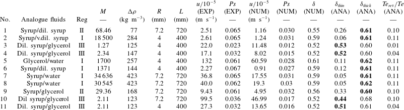
Figure 4 shows the results of three miscible simulations (figure 4
a2,b2,c2) in comparison to three immiscible simulations with identical fluid densities and viscosities (figure 4
a3,b3,c3). The three flow regimes appear qualitatively similar for both miscible and immiscible fluids. Evidently, this conclusion holds true only for sufficiently small diffusivities, in our case for
 $D\leqslant 10^{-8}~\text{m}~\text{s}^{-2}$
or
$D\leqslant 10^{-8}~\text{m}~\text{s}^{-2}$
or
 $Pe>10^{2}$
(see the supplementary material for more details), which is consistent with previous estimates (Petitjeans & Maxworthy Reference Petitjeans and Maxworthy1996; Scoffoni et al.
Reference Scoffoni, Lajeunesse and Homsy2001). Figure 4 also shows that miscible flows tends to have less variability along the interface, which confirms that even a small degree of miscibility notably dampens the growth rate of interface instabilities (e.g. Meiburg et al.
Reference Meiburg, Vanaparthy, Payr and Wilhelm2004).
$Pe>10^{2}$
(see the supplementary material for more details), which is consistent with previous estimates (Petitjeans & Maxworthy Reference Petitjeans and Maxworthy1996; Scoffoni et al.
Reference Scoffoni, Lajeunesse and Homsy2001). Figure 4 also shows that miscible flows tends to have less variability along the interface, which confirms that even a small degree of miscibility notably dampens the growth rate of interface instabilities (e.g. Meiburg et al.
Reference Meiburg, Vanaparthy, Payr and Wilhelm2004).
Direct numerical simulations of the three primary flow regimes (I, II, III) observed in bidirectional tube flow for different viscosity contrasts. Miscible (a2,b2,c2) and immiscible (a3,b3,c3) flows shown in comparison to schematics (a1,b1,b2) reproduced from Stevenson & Blake (Reference Stevenson and Blake1998) (see also online supplementary movies 1–3 showing numerical simulations of experiments from Stevenson & Blake). Simulation snapshots are shown at
 $t=200\times t_{0}$
.
$t=200\times t_{0}$
.
Reproduction of experiment No. 8, treating the fluids as miscible (a) and immiscible (b). Numerical speed profiles (c) taken on marked cross-sections highlighted as red bars in (a) and (b) for miscible (yellow line) and immiscible (red line) flow compared to the analytical solution (black line).
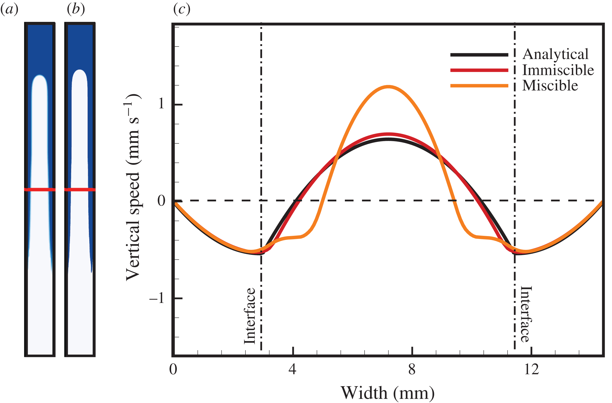
The availability of an analytical solution, at least in the limit of steady core–annular flow, provides a further opportunity to validate our numerical method beyond the benchmarks presented in Qin & Suckale (Reference Qin and Suckale2017). More importantly, it allows us to evaluate the conditions under which miscible flow with low diffusivity behaves approximately as immiscible. In figure 5, we compare the virtual reproduction of experiment No. 8 (figure 5
a) for miscible fluids with its immiscible equivalent (figure 5
b) and with the analytical solution calculated for the same flow parameters. To compare the numerical and analytical results, we take horizontal profiles of the vertical flow speed across the numerical domain in an area of fully developed core–annular flow. At a given flux, the analytical model computes
 $\unicode[STIX]{x1D6FF}$
and the vertical speed curves for both solutions, but it does not allow constraining the flux from first principles. We thus use the flux computed from the numerical simulations as an input to our analytical model. The flow profile of the immiscible simulation agrees remarkably well with the analytical solution corresponding to relatively slow flow in a thick core (figure 5
c) despite the fact that the analytical solution represents steady state whereas the numerical simulation is transient.
$\unicode[STIX]{x1D6FF}$
and the vertical speed curves for both solutions, but it does not allow constraining the flux from first principles. We thus use the flux computed from the numerical simulations as an input to our analytical model. The flow profile of the immiscible simulation agrees remarkably well with the analytical solution corresponding to relatively slow flow in a thick core (figure 5
c) despite the fact that the analytical solution represents steady state whereas the numerical simulation is transient.
The vertical speed profile, however, is significantly modified by fluid miscibility (figure 5 c). The two reasons for this modification are a gradual change in the density and viscosity and a more distributed shear stress in the interfacial zone. Despite the small amount of mixing here, the dynamic consequences are notable in both the increased maximum rise speed in the core and in the narrower upwelling portion of the flow. We find that an exponential variation of viscosity with composition magnifies this effect (see the supplementary material).
3.2 Analysis of virtual experiments
One of the main findings in Stevenson & Blake (Reference Stevenson and Blake1998) is that the Poiseuille number in their experiments is essentially constant (i.e.
 $Ps\approx 0.065$
) at finite viscosity contrast (approximately
$Ps\approx 0.065$
) at finite viscosity contrast (approximately
 $M>10$
). This behaviour stands in stark contrast to the theory of Kazahaya et al. (Reference Kazahaya, Shinohara and Saito1994), which predicts a monotonic increase of
$M>10$
). This behaviour stands in stark contrast to the theory of Kazahaya et al. (Reference Kazahaya, Shinohara and Saito1994), which predicts a monotonic increase of
 $Ps$
with
$Ps$
with
 $M$
. Figure 6 compares the range of experimentally determined
$M$
. Figure 6 compares the range of experimentally determined
 $Ps$
values with the numerical values resulting from our simulations and with the theoretical values calculated from our analytical model in 2-D and 3-D. We also show the theoretical values of Kazahaya et al. (Reference Kazahaya, Shinohara and Saito1994) for comparison. Because our analytical model does not allow us to quantify the rise speed of a transient interface, we instead compute
$Ps$
values with the numerical values resulting from our simulations and with the theoretical values calculated from our analytical model in 2-D and 3-D. We also show the theoretical values of Kazahaya et al. (Reference Kazahaya, Shinohara and Saito1994) for comparison. Because our analytical model does not allow us to quantify the rise speed of a transient interface, we instead compute
 $Ps$
from the average vertical flow speed in the core phase. For consistency, we use the same measure to calculate
$Ps$
from the average vertical flow speed in the core phase. For consistency, we use the same measure to calculate
 $Ps$
from the numerical results. The supplementary material provides a comparison of these two metrics for rise speed and shows that they produce comparable values in our simulations.
$Ps$
from the numerical results. The supplementary material provides a comparison of these two metrics for rise speed and shows that they produce comparable values in our simulations.
Plot of the Poiseuille number,
 $Ps$
, against the decadal logarithm of viscosity ratio
$Ps$
, against the decadal logarithm of viscosity ratio
 $M$
, for numerical simulations (green stars), analytical model predictions (black circles for 3-D, blue squares for 2-D), and the range of analogue experiments (grey shading) performed by Stevenson & Blake (Reference Stevenson and Blake1998). Analytical solution of Kazahaya et al. (Reference Kazahaya, Shinohara and Saito1994) shown for comparison (black line). The numerical simulations shown are the reproduction of the experiments of Stevenson & Blake (Reference Stevenson and Blake1998), also shown in figure 3, and are all miscible.
$M$
, for numerical simulations (green stars), analytical model predictions (black circles for 3-D, blue squares for 2-D), and the range of analogue experiments (grey shading) performed by Stevenson & Blake (Reference Stevenson and Blake1998). Analytical solution of Kazahaya et al. (Reference Kazahaya, Shinohara and Saito1994) shown for comparison (black line). The numerical simulations shown are the reproduction of the experiments of Stevenson & Blake (Reference Stevenson and Blake1998), also shown in figure 3, and are all miscible.
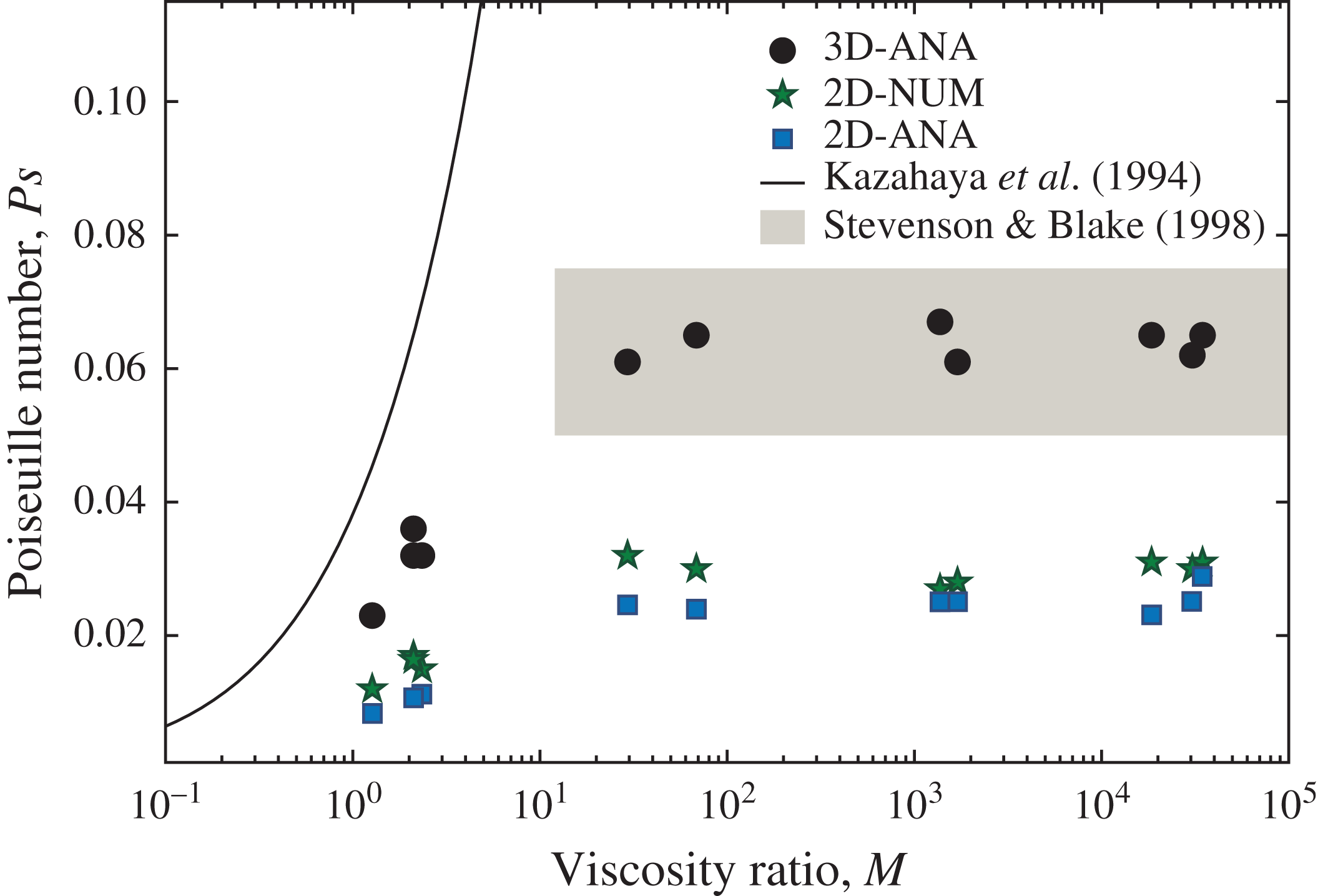
Figure 6 shows that our 3-D analytical model (black dots) agrees well with the range of observed
 $Ps$
numbers (grey shaded) reported by Stevenson & Blake (Reference Stevenson and Blake1998) for
$Ps$
numbers (grey shaded) reported by Stevenson & Blake (Reference Stevenson and Blake1998) for
 $M>10$
. It also quantifies the difference between
$M>10$
. It also quantifies the difference between
 $Ps$
in 2-D (blue squares) versus 3-D (black circles). In 3-D, the rise speed is approximately twice as fast as in 2-D. The 2-D analytical estimates (blue squares) agree well with the 2-D numerical estimates (green stars). All three pieces, the measured data, the analytical values and the numerical outcomes, indicate that
$Ps$
in 2-D (blue squares) versus 3-D (black circles). In 3-D, the rise speed is approximately twice as fast as in 2-D. The 2-D analytical estimates (blue squares) agree well with the 2-D numerical estimates (green stars). All three pieces, the measured data, the analytical values and the numerical outcomes, indicate that
 $Ps$
levels off with increasing
$Ps$
levels off with increasing
 $M$
, in contrast to the findings of Kazahaya et al. (Reference Kazahaya, Shinohara and Saito1994).
$M$
, in contrast to the findings of Kazahaya et al. (Reference Kazahaya, Shinohara and Saito1994).
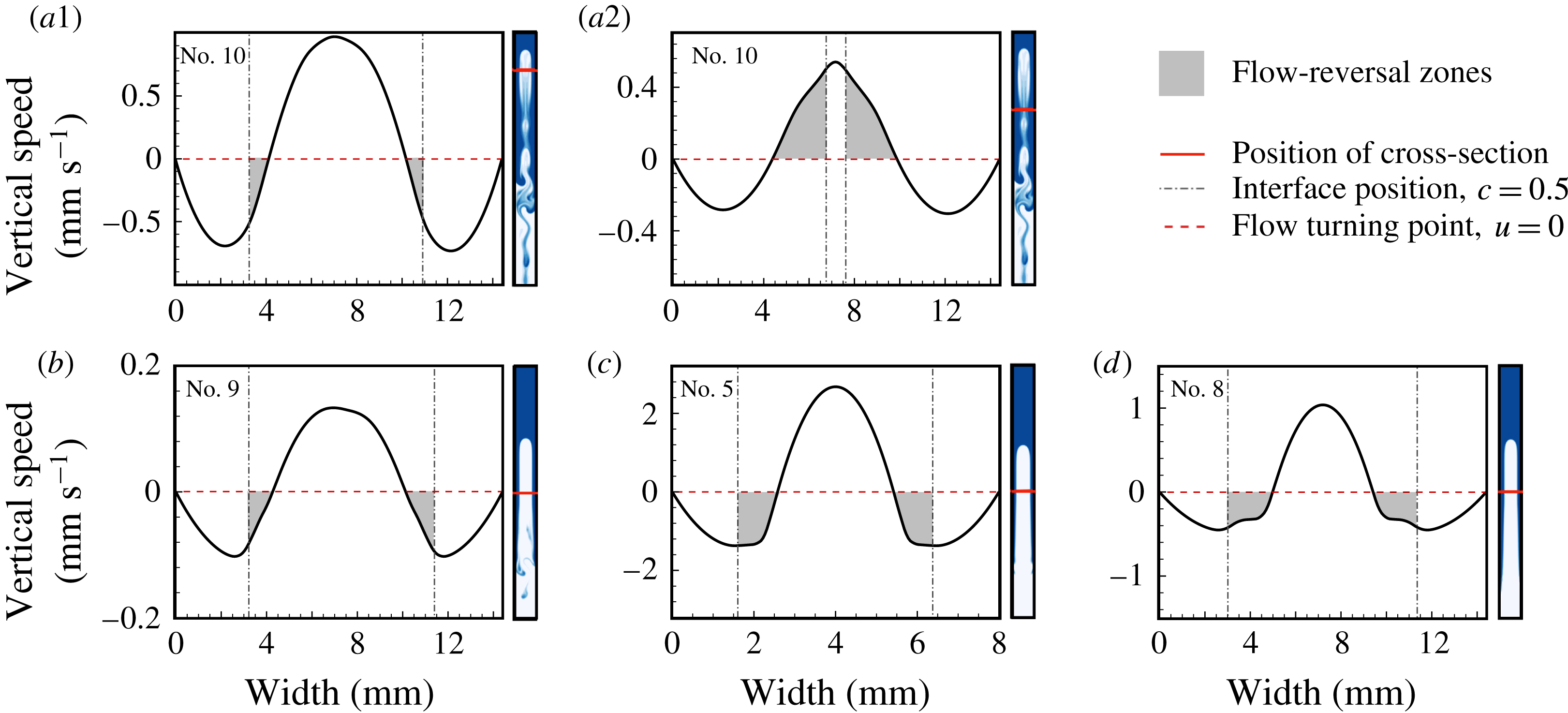
Stevenson & Blake (Reference Stevenson and Blake1998) hypothesized that the disconnection between observed
 $Ps$
values and model predictions of Kazahaya et al. (Reference Kazahaya, Shinohara and Saito1994) is related to their assumption that the interface between the ascending and descending fluid is immobile (i.e.
$Ps$
values and model predictions of Kazahaya et al. (Reference Kazahaya, Shinohara and Saito1994) is related to their assumption that the interface between the ascending and descending fluid is immobile (i.e.
 $u_{i}=0$
). Our virtual reproductions of the analogue experiments allow us to test this hypothesis. In figure 7, we plot vertical flow speed profiles across four different experiments: No. 10 (figure 7
a), No. 9 (figure 7
b), No. 5 (figure 7
c) and No. 8 (figure 7
d). These four experiments with increasing viscosity ratios represent the three different flow regimes indicated in figure 4. We arrange the experiments in this order to highlight the change in interface speed with increasing viscosity contrast. Our results give clear confirmation of the hypothesis of Stevenson & Blake (Reference Stevenson and Blake1998), showing that the interface is indeed not stationary.
$u_{i}=0$
). Our virtual reproductions of the analogue experiments allow us to test this hypothesis. In figure 7, we plot vertical flow speed profiles across four different experiments: No. 10 (figure 7
a), No. 9 (figure 7
b), No. 5 (figure 7
c) and No. 8 (figure 7
d). These four experiments with increasing viscosity ratios represent the three different flow regimes indicated in figure 4. We arrange the experiments in this order to highlight the change in interface speed with increasing viscosity contrast. Our results give clear confirmation of the hypothesis of Stevenson & Blake (Reference Stevenson and Blake1998), showing that the interface is indeed not stationary.
A finite interface speed implies that the turning point between upward- and downward-oriented flow shifts into one of the two fluids. At low viscosity contrast (flow regime III), this shift may occur in either the ascending or in the descending fluid (see figure 7
a1,a2) and is linked to transient effects. For flow regimes I and II, the shift occurs in the ascending fluid in all simulations (figure 7
b–d). This finding implies that, at intermediate to high viscosity contrasts (i.e.
 $M>10$
), a portion of the buoyant fluid in fact flows downwards in the tube – a phenomenon commonly referred to as flow reversal or backflow.
$M>10$
), a portion of the buoyant fluid in fact flows downwards in the tube – a phenomenon commonly referred to as flow reversal or backflow.
Zones of flow reversal (grey shaded) in bidirectional flow experiments on horizontal profiles of vertical speed,
 $u(r)$
, along cross-sections through virtual experiments marked by red bars across reported flow patterns. (a1,a2) Profiles of experiment No. 10, low viscosity contrast
$u(r)$
, along cross-sections through virtual experiments marked by red bars across reported flow patterns. (a1,a2) Profiles of experiment No. 10, low viscosity contrast
 $M$
, flow regime III. (b) Experiment No. 9, intermediate
$M$
, flow regime III. (b) Experiment No. 9, intermediate
 $M$
, regime II. (c) Experiment No. 5, high
$M$
, regime II. (c) Experiment No. 5, high
 $M$
, regime I. (d) Experiment No. 8, very high
$M$
, regime I. (d) Experiment No. 8, very high
 $M$
, regime I.
$M$
, regime I.
To quantify flow reversal more systematically, we compute the ratio between the flux in a given phase,
 $Te$
, and the flow-reversal flux in the same phase,
$Te$
, and the flow-reversal flux in the same phase,
 $Te_{rev}$
, which we define as
$Te_{rev}$
, which we define as
 $$\begin{eqnarray}\displaystyle Te_{rev}=\left|\int _{\unicode[STIX]{x1D6FF}_{rev}}^{\unicode[STIX]{x1D6FF}}2\unicode[STIX]{x03C0}ru_{a}(r)\,\text{d}r\right|, & & \displaystyle\end{eqnarray}$$
where
 $\unicode[STIX]{x1D6FF}_{rev}$
is the point at which the vertical flow speed in the ascending fluid crosses zero,
$\unicode[STIX]{x1D6FF}_{rev}$
is the point at which the vertical flow speed in the ascending fluid crosses zero,
 $u_{a}(\unicode[STIX]{x1D6FF}_{rev})=0$
. With this definition,
$u_{a}(\unicode[STIX]{x1D6FF}_{rev})=0$
. With this definition,
 $Te_{rev}$
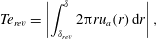
quantifies the flux of ascending fluid that is trapped in the flow-reversal zone. Figure 8 shows the analytically predicted flow-reversal flux as a function of dimensionless model parameters. Figure 8(a) shows its dependence on the core radius,
$Te_{rev}$
quantifies the flux of ascending fluid that is trapped in the flow-reversal zone. Figure 8 shows the analytically predicted flow-reversal flux as a function of dimensionless model parameters. Figure 8(a) shows its dependence on the core radius,
 $\unicode[STIX]{x1D6FF}$
, for different viscosity contrasts. For viscosity contrasts
$\unicode[STIX]{x1D6FF}$
, for different viscosity contrasts. For viscosity contrasts
 $M>10$
, the experimentally observed core radii (
$M>10$
, the experimentally observed core radii (
 $\unicode[STIX]{x1D6FF}\approx 0.6$
) cluster just below the values resulting in maximum flow reversal. In figure 8(b), we plot the ratio of flow reversal to total flux, again as a function of
$\unicode[STIX]{x1D6FF}\approx 0.6$
) cluster just below the values resulting in maximum flow reversal. In figure 8(b), we plot the ratio of flow reversal to total flux, again as a function of
 $\unicode[STIX]{x1D6FF}$
and
$\unicode[STIX]{x1D6FF}$
and
 $M$
.
$M$
.
We find that at intermediate and high viscosity contrast,
 $Te_{rev}/Te$
is mostly insensitive to the viscosity ratio for sufficiently high core radius. In fact, for
$Te_{rev}/Te$
is mostly insensitive to the viscosity ratio for sufficiently high core radius. In fact, for
 $M\gtrapprox 10$
and
$M\gtrapprox 10$
and
 $\unicode[STIX]{x1D6FF}\gtrapprox 0.4$
, the flow reversal takes place in the ascending phase, and both the total and flow-reversal flux approach the asymptotic limit of
$\unicode[STIX]{x1D6FF}\gtrapprox 0.4$
, the flow reversal takes place in the ascending phase, and both the total and flow-reversal flux approach the asymptotic limit of
 $M\rightarrow \infty$
:
$M\rightarrow \infty$
:
 $$\begin{eqnarray}\displaystyle & \displaystyle Te(\unicode[STIX]{x1D6FF},\unicode[STIX]{x1D6FC}=0,M\rightarrow \infty )=\frac{\unicode[STIX]{x03C0}}{8}[1-4\unicode[STIX]{x1D6FF}^{2}+(3-4\log \unicode[STIX]{x1D6FF})\unicode[STIX]{x1D6FF}^{4}], & \displaystyle\end{eqnarray}$$
 $$\begin{eqnarray}\displaystyle & \displaystyle Te_{rev}(\unicode[STIX]{x1D6FF},\unicode[STIX]{x1D6FC}=0,M\rightarrow \infty )=\frac{\unicode[STIX]{x03C0}}{8}\frac{\unicode[STIX]{x1D6FF}^{4}(2\unicode[STIX]{x1D6FF}^{2}\log \unicode[STIX]{x1D6FF}-\unicode[STIX]{x1D6FF}^{2}+1)^{2}}{(\unicode[STIX]{x1D6FF}^{2}-1)^{2}}\quad \text{for }\unicode[STIX]{x1D6FF}>\unicode[STIX]{x1D6FF}_{rev}. & \displaystyle\end{eqnarray}$$
The insight that the interface between the two fluids is inherently dynamic does not yet explain why
 $Ps$
remains approximately constant with increasing
$Ps$
remains approximately constant with increasing
 $M$
. To find an explanation, we return to (2.14) in § 2.1. It states that the function
$M$
. To find an explanation, we return to (2.14) in § 2.1. It states that the function
 $Te(\unicode[STIX]{x1D6FF})$
has a quadratic component, which suggests that two valid solutions for
$Te(\unicode[STIX]{x1D6FF})$
has a quadratic component, which suggests that two valid solutions for
 $\unicode[STIX]{x1D6FF}$
may exist for a given flux. The existence of multiple solutions is a common feature of gravity dominated multiphase flows, yet it does not necessarily imply that both solutions are realized in the laboratory (e.g. Landman Reference Landman1991; Brauner Reference Brauner1998; Ullmann et al.
Reference Ullmann, Zamir, Ludmer and Brauner2003; Picchi & Poesio Reference Picchi and Poesio2016), or indeed in natural systems.
$\unicode[STIX]{x1D6FF}$
may exist for a given flux. The existence of multiple solutions is a common feature of gravity dominated multiphase flows, yet it does not necessarily imply that both solutions are realized in the laboratory (e.g. Landman Reference Landman1991; Brauner Reference Brauner1998; Ullmann et al.
Reference Ullmann, Zamir, Ludmer and Brauner2003; Picchi & Poesio Reference Picchi and Poesio2016), or indeed in natural systems.
In figure 9, we illustrate the two valid core–annular solutions for experiment No. 5 (see table 1). At the experimentally observed dimensionless flux,
 $Te=0.075$
, our model predicts two solutions for the core radius, the thick-core (
$Te=0.075$
, our model predicts two solutions for the core radius, the thick-core (
 $\unicode[STIX]{x1D6FF}_{thick}$
, blue diamond) and the thin-core solution (
$\unicode[STIX]{x1D6FF}_{thick}$
, blue diamond) and the thin-core solution (
 $\unicode[STIX]{x1D6FF}_{thin}$
, red triangle). The two corresponding flow profiles, shown from the centre of the tube to the wall in figure 9(b,c), highlight that the same overall flux can be accommodated by either a thin, rapidly ascending core with a thick annulus, or through a thick, slowly ascending core with a thin annulus. Interestingly, both solutions are far removed from the point of maximum flux or flooding point (yellow
$\unicode[STIX]{x1D6FF}_{thin}$
, red triangle). The two corresponding flow profiles, shown from the centre of the tube to the wall in figure 9(b,c), highlight that the same overall flux can be accommodated by either a thin, rapidly ascending core with a thick annulus, or through a thick, slowly ascending core with a thin annulus. Interestingly, both solutions are far removed from the point of maximum flux or flooding point (yellow
 $\times$
).
$\times$
).
(a) Dimensionless flow-reversal flux in the ascending phase,
 $Te_{rev}$
, as a function of the core radius
$Te_{rev}$
, as a function of the core radius
 $\unicode[STIX]{x1D6FF}$
. (b) Normalized dimensionless flow-reversal flux in the ascending phase,
$\unicode[STIX]{x1D6FF}$
. (b) Normalized dimensionless flow-reversal flux in the ascending phase,
 $Te_{rev}$
, scaled by the net dimensionless flux,
$Te_{rev}$
, scaled by the net dimensionless flux,
 $Te$
, as a function of the core radius,
$Te$
, as a function of the core radius,
 $\unicode[STIX]{x1D6FF}$
.
$\unicode[STIX]{x1D6FF}$
.
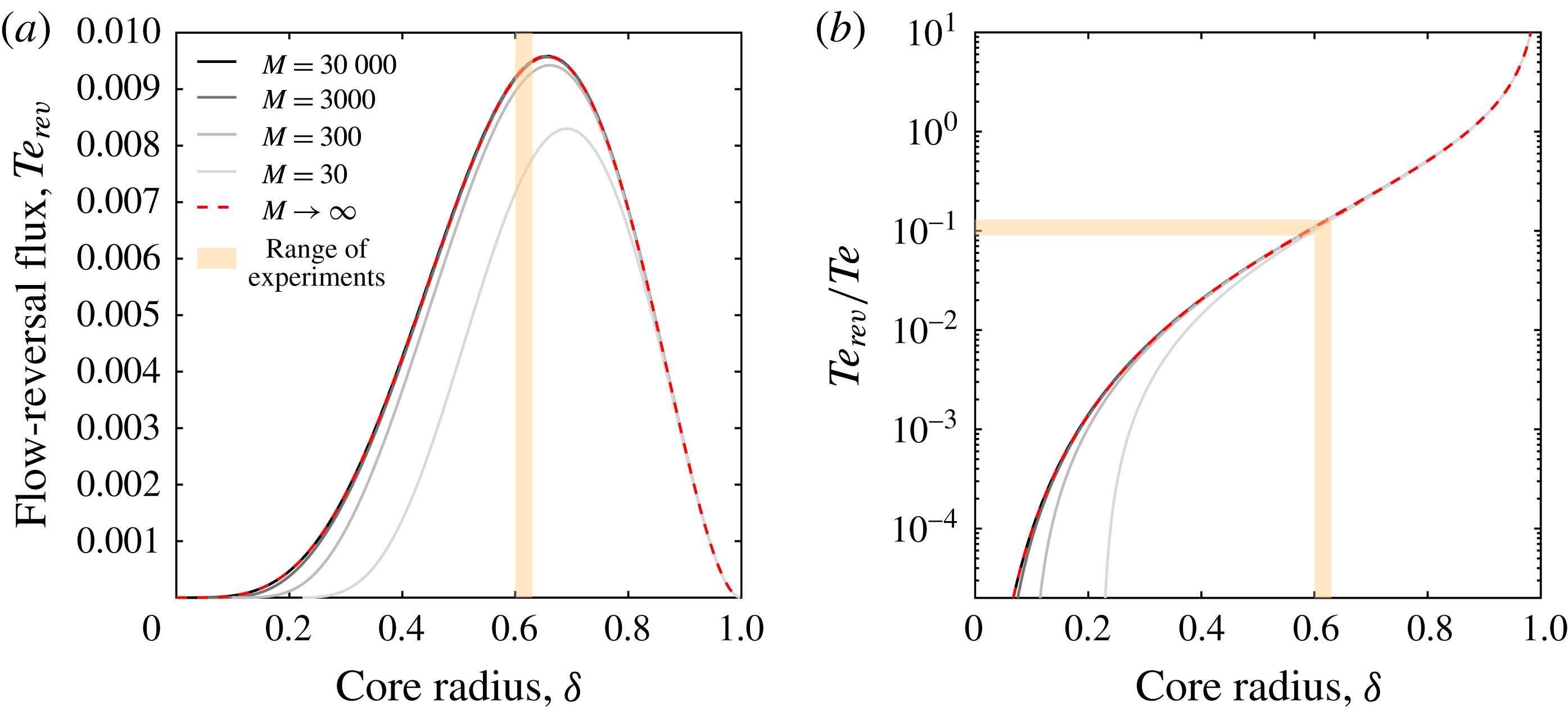
Table 1 lists the two analytically computed core radii at the
 $Te$
values inferred from the reported terminal rise speeds in all 11 experiments. The solutions compatible with Stevenson & Blake’s (Reference Stevenson and Blake1998) experimental and our numerical outcomes are printed in bold. We find that all experiments with viscosity contrasts of
$Te$
values inferred from the reported terminal rise speeds in all 11 experiments. The solutions compatible with Stevenson & Blake’s (Reference Stevenson and Blake1998) experimental and our numerical outcomes are printed in bold. We find that all experiments with viscosity contrasts of
 $M>10$
select the thick-core solution,
$M>10$
select the thick-core solution,
 $\unicode[STIX]{x1D6FF}_{thick}$
. The thin-core solution,
$\unicode[STIX]{x1D6FF}_{thick}$
. The thin-core solution,
 $\unicode[STIX]{x1D6FF}_{thin}$
, may be pertinent for the experiments with small viscosity contrasts (experiments No. 3, No. 4, No. 10 and No. 11), but these cases do not exhibit stable core–annular flow, and the applicability of the analytical model is thus questionable.
$\unicode[STIX]{x1D6FF}_{thin}$
, may be pertinent for the experiments with small viscosity contrasts (experiments No. 3, No. 4, No. 10 and No. 11), but these cases do not exhibit stable core–annular flow, and the applicability of the analytical model is thus questionable.
Figure 10 shows analytical flux solutions for all experiments as a function of core radius and viscosity contrast. For each
 $Te$
-
$Te$
-
 $\unicode[STIX]{x1D6FF}$
curve in figure 10(a), we mark the solution that is realized in experiments (
$\unicode[STIX]{x1D6FF}$
curve in figure 10(a), we mark the solution that is realized in experiments (
 $\unicode[STIX]{x1D6FF}_{thick}$
, red triangle;
$\unicode[STIX]{x1D6FF}_{thick}$
, red triangle;
 $\unicode[STIX]{x1D6FF}_{thin}$
, blue diamond). We show curves for experiments No. 3, No. 4, No. 10 and No. 11 as light-grey lines to convey that our analytical model is questionable for these cases. The experiments with
$\unicode[STIX]{x1D6FF}_{thin}$
, blue diamond). We show curves for experiments No. 3, No. 4, No. 10 and No. 11 as light-grey lines to convey that our analytical model is questionable for these cases. The experiments with
 $M>3$
(solid lines) all cluster around
$M>3$
(solid lines) all cluster around
 $\unicode[STIX]{x1D6FF}\approx 0.61$
and
$\unicode[STIX]{x1D6FF}\approx 0.61$
and
 $Te\approx 0.075$
. Hence, the scatter in the
$Te\approx 0.075$
. Hence, the scatter in the
 $Ps$
number in Stevenson & Blake (Reference Stevenson and Blake1998) (see figure 6) is not related entirely to uncertainty of measurement but also reflects the fact that
$Ps$
number in Stevenson & Blake (Reference Stevenson and Blake1998) (see figure 6) is not related entirely to uncertainty of measurement but also reflects the fact that
 $Te$
values at different
$Te$
values at different
 $M>3$
are very similar but not identical (see figure 10
b). For experiments with a viscosity ratio close to unity (light-grey lines),
$M>3$
are very similar but not identical (see figure 10
b). For experiments with a viscosity ratio close to unity (light-grey lines),
 $Te$
assumes much lower values (figure 10
b), and the two possible solutions are no longer clearly distinct.
$Te$
assumes much lower values (figure 10
b), and the two possible solutions are no longer clearly distinct.
This analysis suggests that the dichotomy in
 $Ps$
number observed by Stevenson & Blake (Reference Stevenson and Blake1998) and reproduced in figure 6 reflects a shift from thick-core core–annular flow (flow regimes I and II) to unstable overturn flow (flow regime III). Contrary to the thin-core solution, the thick-core solution exhibits approximately constant core thickness over a large range of
$Ps$
number observed by Stevenson & Blake (Reference Stevenson and Blake1998) and reproduced in figure 6 reflects a shift from thick-core core–annular flow (flow regimes I and II) to unstable overturn flow (flow regime III). Contrary to the thin-core solution, the thick-core solution exhibits approximately constant core thickness over a large range of
 $M$
(see figure 10
a), which means that a constant
$M$
(see figure 10
a), which means that a constant
 $Te$
translates to a constant
$Te$
translates to a constant
 $Ps$
(2.12). If any of the experiments exhibited the thin-core solution,
$Ps$
(2.12). If any of the experiments exhibited the thin-core solution,
 $Ps$
would increase with
$Ps$
would increase with
 $M$
.
$M$
.
(a) Transport number,
 $Te$
, and interface speed,
$Te$
, and interface speed,
 $u_{i}$
, as a function of the dimensionless core radius,
$u_{i}$
, as a function of the dimensionless core radius,
 $\unicode[STIX]{x1D6FF}$
, for experiment No. 5 (
$\unicode[STIX]{x1D6FF}$
, for experiment No. 5 (
 $M=1700$
). (b,c) Dimensionless velocity profiles of the thin-core,
$M=1700$
). (b,c) Dimensionless velocity profiles of the thin-core,
 $\unicode[STIX]{x1D6FF}_{thin}$
, and thick-core,
$\unicode[STIX]{x1D6FF}_{thin}$
, and thick-core,
 $\unicode[STIX]{x1D6FF}_{thick}$
, solutions at
$\unicode[STIX]{x1D6FF}_{thick}$
, solutions at
 $Te=0.075$
. We estimate
$Te=0.075$
. We estimate
 $Te$
based on the experimental rise speed.
$Te$
based on the experimental rise speed.
3.3 Simulations of persistent exchange flow
The result that only the thick-core solution is realized in core–annular flow at finite viscosity contrast in closed tubes raises the question whether this flow configuration is generally preferable. At very high viscosity contrast,
 $M>10\,000$
, the thin-core solution entails an extremely thin core (e.g. see experiments No. 2, No. 7 and No. 8 in table 1), which would be highly prone to wave bridging and flow collapse (e.g. Barnea Reference Barnea1987). In the limit of extreme to infinite viscosity contrast, it is hence likely that the thick-core solution is generally preferable.
$M>10\,000$
, the thin-core solution entails an extremely thin core (e.g. see experiments No. 2, No. 7 and No. 8 in table 1), which would be highly prone to wave bridging and flow collapse (e.g. Barnea Reference Barnea1987). In the limit of extreme to infinite viscosity contrast, it is hence likely that the thick-core solution is generally preferable.
Determining the physical relevance of the two solutions based on core radius alone, however, becomes unsatisfactory at high to intermediate viscosity contrast, when the core radii become increasingly comparable. In this section, we explore the possibility that the physically pertinent solution may be controlled not only by the material parameters but also by the in- and outflux boundaries, an idea raised but not explored in detail by Barnea & Taitel (Reference Barnea and Taitel1985). The experiments of Stevenson & Blake (Reference Stevenson and Blake1998) were performed in closed test tubes, which are significantly different from natural systems where exchange flow is typically the consequence of continued flux.
To generalize insights from closed to open systems, we perform simulations with open boundaries at the top and the base of the model domain. All the simulations discussed in this section are forced by a time-independent inflow condition imposed along the base of the domain and set according to the analytical speed profile in 2-D (see (8) and (9) in the supplementary material). This choice of boundary condition automatically imposes a certain flux,
 $Te$
. We test both thin- and thick-core influx by applying either
$Te$
. We test both thin- and thick-core influx by applying either
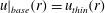 $u|_{base}(r)=u_{thin}(r)$
or
$u|_{base}(r)=u_{thin}(r)$
or
 $u|_{base}(r)=u_{thick}(r)$
. Both solutions entail the same flux,
$u|_{base}(r)=u_{thick}(r)$
. Both solutions entail the same flux,
 $Te$
. We continue to enforce a no-slip condition (
$Te$
. We continue to enforce a no-slip condition (
 $\boldsymbol{v}|_{side}=0$
) along the side walls. For the outflow condition and the initial interface position, we consider four different cases (see figure 11).
$\boldsymbol{v}|_{side}=0$
) along the side walls. For the outflow condition and the initial interface position, we consider four different cases (see figure 11).
(a)
 $Te$
–
$Te$
–
 $\unicode[STIX]{x1D6FF}$
curves for all experiments listed in table 1. The plot shows 10 instead of 11 curves, because experiments No. 10 and No. 11 have the same viscosity ratio. Numerically and experimentally realized core radii are highlighted as red triangles (thick core) and blue diamonds (thin core). (b) Transport number,
$\unicode[STIX]{x1D6FF}$
curves for all experiments listed in table 1. The plot shows 10 instead of 11 curves, because experiments No. 10 and No. 11 have the same viscosity ratio. Numerically and experimentally realized core radii are highlighted as red triangles (thick core) and blue diamonds (thin core). (b) Transport number,
 $Te$
, against the viscosity ratio,
$Te$
, against the viscosity ratio,
 $M$
, as computed from the analytical model for the experiments of Stevenson & Blake (Reference Stevenson and Blake1998).
$M$
, as computed from the analytical model for the experiments of Stevenson & Blake (Reference Stevenson and Blake1998).
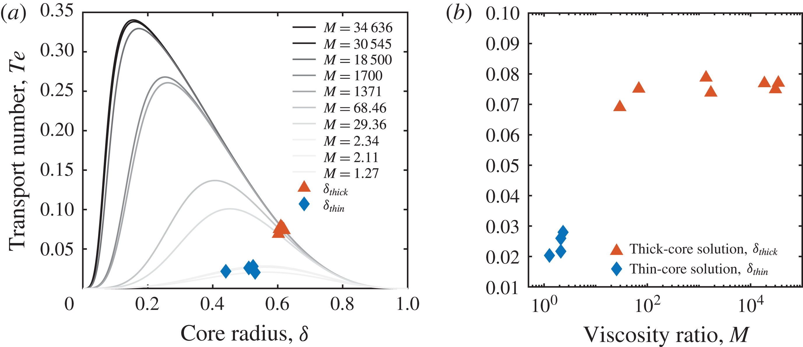
Snapshots of numerical simulations forced with thick- and thin-core analytical solutions at the inlet. Material properties are identical to those in experiment No. 9 of Stevenson & Blake (Reference Stevenson and Blake1998). Results are shown for: fixed outlet boundary, enforcing the analytical model at the top boundary for thick- (a1–a3) and thin-core (b1–b3) solutions; free outlet, stress-free top boundary allowing free flow through the top, starting from fully developed bidirectional configuration (d1–e3), and with a transient front moving through the domain (g1–h3); the same as in the previous case but with miscible fluids (k1–l3). Horizontal profiles of vertical speed (c,f,j,m) show numerical solutions approaching either thin- or thick-core analytical solutions depending on boundary conditions and fluid miscibility. See also supplementary movie 4 for a simulation of (h1–h3).
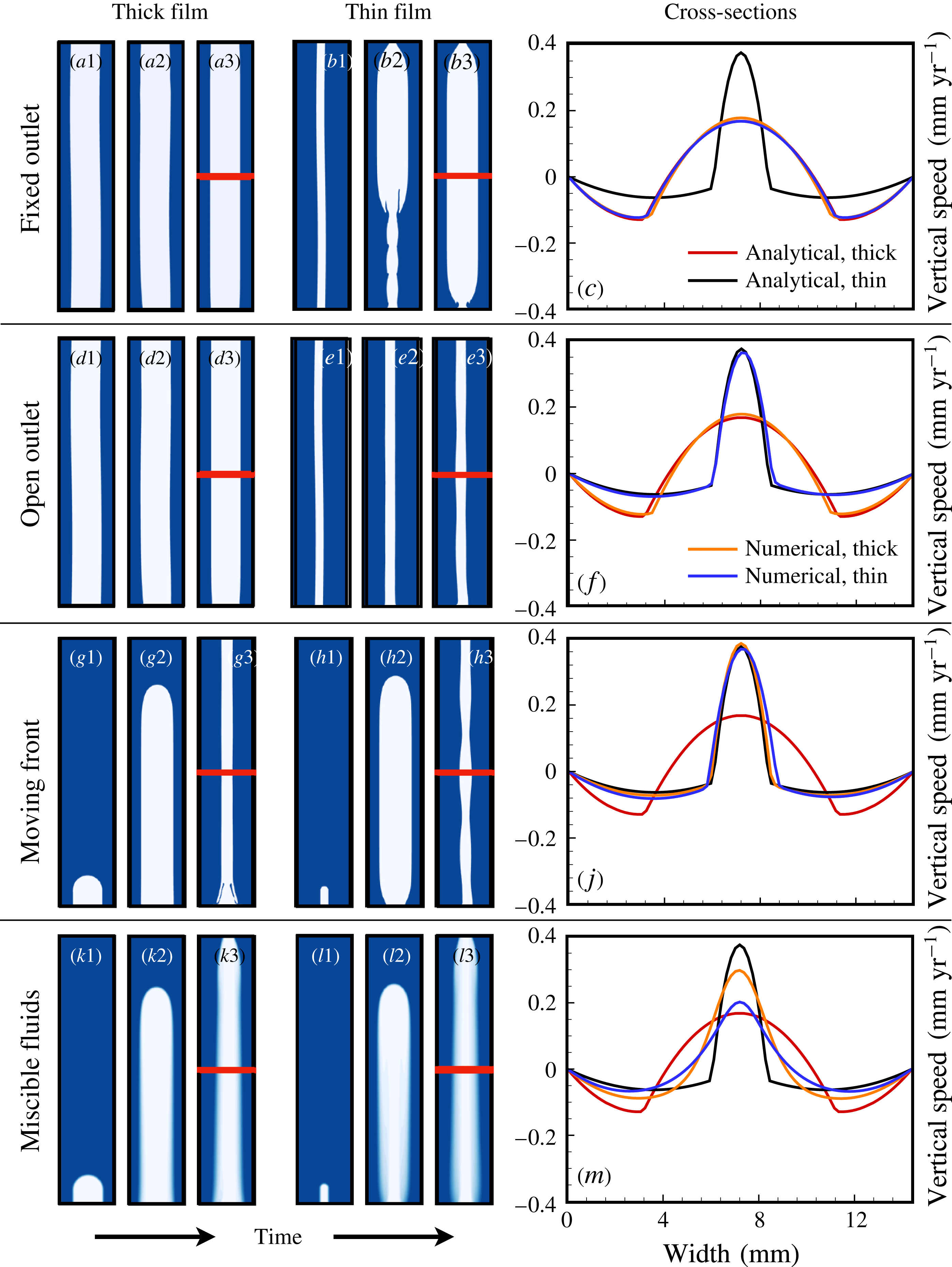
For the first case (figure 11
a1–c), we impose a fixed outflow condition along the top boundary. We set the same analytical flow profile for the top and the base of the domain, that is
 $u|_{base}(r)=u|_{top}(r)=u_{thick}(r)$
and
$u|_{base}(r)=u|_{top}(r)=u_{thick}(r)$
and
 $u|_{base}(r)=u|_{top}(r)=u_{thin}(r)$
, respectively. We also initiate the concentration field to the corresponding geometry extended through the whole domain (see figure 11
a1,b1). This choice implies that the interface is pinned at both the top and bottom of the domain. Although this set-up is clearly contrived, it is an interesting end-member case for understanding the respective stability of the two solutions. Intuitively, one might expect that, if forced by the analytical solution on both ends, the flow field in the domain will remain close to that solution. Figure 11(c) shows that this is clearly not the case. Although both interfaces are slightly wavy initially (figure 11
a1,b1), the thick-core solution stabilizes (figure 11
a3). However, the thin-core case begins transitioning to the thick-core flow field from the top boundary downwards almost immediately after the onset of flow (figure 11
b2,b3). The speed profiles taken in the middle of the domain, where the flow is approximately at steady state, confirm that both simulations closely approach the analytical thick-core solution (figure 11
c).
$u|_{base}(r)=u|_{top}(r)=u_{thin}(r)$
, respectively. We also initiate the concentration field to the corresponding geometry extended through the whole domain (see figure 11
a1,b1). This choice implies that the interface is pinned at both the top and bottom of the domain. Although this set-up is clearly contrived, it is an interesting end-member case for understanding the respective stability of the two solutions. Intuitively, one might expect that, if forced by the analytical solution on both ends, the flow field in the domain will remain close to that solution. Figure 11(c) shows that this is clearly not the case. Although both interfaces are slightly wavy initially (figure 11
a1,b1), the thick-core solution stabilizes (figure 11
a3). However, the thin-core case begins transitioning to the thick-core flow field from the top boundary downwards almost immediately after the onset of flow (figure 11
b2,b3). The speed profiles taken in the middle of the domain, where the flow is approximately at steady state, confirm that both simulations closely approach the analytical thick-core solution (figure 11
c).
The second case (figure 11
d1–f) represents a scenario with open outflow across a stress-free top boundary, which we enforce by setting
 $p|_{top}=\text{const.}$
, and
$p|_{top}=\text{const.}$
, and
 $\unicode[STIX]{x2202}\boldsymbol{v}/\unicode[STIX]{x2202}z|_{top}=\mathbf{0}$
. The flow field across the upper boundary thus evolves over time, and the interface will move freely with the outflow. The initial position of the interface is identical to that in the first case (figure 11
d1,e1). The emerging flow fields correspond closely to the analytical solution imposed at the base of the domain. A thick-core inflow leads to a stable thick-core configuration (figure 11
d3) and a thin-core inflow leads to a stable thin-core configuration (figure 11
e3). This case demonstrates that the thin-core solution is a physically relevant flow configuration, at least at a viscosity contrast of
$\unicode[STIX]{x2202}\boldsymbol{v}/\unicode[STIX]{x2202}z|_{top}=\mathbf{0}$
. The flow field across the upper boundary thus evolves over time, and the interface will move freely with the outflow. The initial position of the interface is identical to that in the first case (figure 11
d1,e1). The emerging flow fields correspond closely to the analytical solution imposed at the base of the domain. A thick-core inflow leads to a stable thick-core configuration (figure 11
d3) and a thin-core inflow leads to a stable thin-core configuration (figure 11
e3). This case demonstrates that the thin-core solution is a physically relevant flow configuration, at least at a viscosity contrast of
 $M\approx 30$
. Together with the first case, these simulations confirm that boundary conditions indeed have a profound influence on which mathematically valid flow configuration is realized in practice, as suggested by Barnea & Taitel (Reference Barnea and Taitel1985).
$M\approx 30$
. Together with the first case, these simulations confirm that boundary conditions indeed have a profound influence on which mathematically valid flow configuration is realized in practice, as suggested by Barnea & Taitel (Reference Barnea and Taitel1985).
One advantage of the variable over the fixed outflow case is that we can now consider a different initial interface position. In our third case (figure 11 g1–j), we initiate a closed interface confined to the vicinity of the lower boundary (figure 11 g1,h1), ensuring that the core radius corresponds to the analytical solution enforced at inflow. In these simulations, the interface movement through the domain is similar to that in the experiments (figure 11 g2,h2), but the interface eventually leaves the computational domain through the upper boundary.
Immediately after onset, both the thick- and thin-core flows approach the thick-core solution (figure 11 g2,h2). However, as soon as the interface intersects with the upper boundary, the flow in both simulations collapses back to the thin-core solution (figure 10 g3,h3). This case demonstrates not only that the preferable flow configuration depends on the boundary conditions, but also that a transient disruption on one boundary, such as the passage of the interface through the top, can trigger a switch in the flow configuration that propagates across the entire domain.
Because the analytical solution strictly applies only to the immiscible limit, we have thus far considered only immiscible fluids in this section. In the fourth case (figure 11
k1–m), we repeat the third case with miscible fluids at high
 $Pe$
. Initially, the thin-core flow widens immediately (figure 11
l2), but both flow configurations collapse back to a thin core once the interface passes through the upper boundary (figure 11
k3,l3). The vertical speed profiles are reminiscent of the thin-core solution but more spread out (figure 11
m). The interface remains less wavy throughout, which supports the theoretical expectation that mixing stabilizes core–annular flow against interface waves (e.g. Meiburg et al.
Reference Meiburg, Vanaparthy, Payr and Wilhelm2004).
$Pe$
. Initially, the thin-core flow widens immediately (figure 11
l2), but both flow configurations collapse back to a thin core once the interface passes through the upper boundary (figure 11
k3,l3). The vertical speed profiles are reminiscent of the thin-core solution but more spread out (figure 11
m). The interface remains less wavy throughout, which supports the theoretical expectation that mixing stabilizes core–annular flow against interface waves (e.g. Meiburg et al.
Reference Meiburg, Vanaparthy, Payr and Wilhelm2004).
4 Discussion
4.1 Theoretical implications
Laboratory experiments have provided invaluable insights into the dynamics of buoyancy-driven exchange flows, but they inevitably simplify the more complex flow problem they intend to represent. One aspect in which many analogue models of exchange flow differ fundamentally from natural or industrial systems is that bidirectional flow occurs only as transient behaviour until a steady state of complete inversion of the two fluids is reached (Stevenson & Blake Reference Stevenson and Blake1998; Huppert & Hallworth Reference Huppert and Hallworth2007; Beckett et al. Reference Beckett, Mader, Phillips, Rust and Witham2011; Palma, Blake & Calder Reference Palma, Blake and Calder2011). The steady state in the laboratory is hence very different from that in most natural or industrial problems of interest. Our analysis suggests that this difference may be consequential, because closed systems realize only a subset of the possible flow solutions that occur in open systems. Experiments in closed domains may hence systematically underestimate the dynamic variability of open-system flow.
We derive a simple analytical model that allows us to characterize the two steady-state solutions for core–annular flow. These two solutions refer to the same magnitude of flux, or
 $Te$
, but differ in their core radii,
$Te$
, but differ in their core radii,
 $\unicode[STIX]{x1D6FF}_{thick}$
and
$\unicode[STIX]{x1D6FF}_{thick}$
and
 $\unicode[STIX]{x1D6FF}_{thin}$
, flow speed profile, and degree of flow reversal. We also predict the flux curve,
$\unicode[STIX]{x1D6FF}_{thin}$
, flow speed profile, and degree of flow reversal. We also predict the flux curve,
 $Te(\unicode[STIX]{x1D6FF})$
, based only on the fluid properties and tube radius. The model does not require a fitting parameter to match experimental or numerical data, but it predicts neither the total flux nor the solution that is realized to achieve that flux. In fact, our analysis implies that it is not possible to predict these two outcome variables based on the fluid properties and the tube geometry alone, because the boundary conditions play an important role in determining these variables.
$Te(\unicode[STIX]{x1D6FF})$
, based only on the fluid properties and tube radius. The model does not require a fitting parameter to match experimental or numerical data, but it predicts neither the total flux nor the solution that is realized to achieve that flux. In fact, our analysis implies that it is not possible to predict these two outcome variables based on the fluid properties and the tube geometry alone, because the boundary conditions play an important role in determining these variables.
Huppert & Hallworth (Reference Huppert and Hallworth2007) suggested that buoyancy-driven exchange flow in vertical pipes tends to maximize flux, which would be equivalent to maximizing
 $Te$
. This argument implies that the flux should be at the flooding point for most or all of the experiments (figure 10
a), because the non-dimensional viscous dissipation is directly proportional to the flux magnitude
$Te$
. This argument implies that the flux should be at the flooding point for most or all of the experiments (figure 10
a), because the non-dimensional viscous dissipation is directly proportional to the flux magnitude
 $Te$
(see the supplementary material). This prediction, however, is at odds with both the experimental and the numerical results discussed here. Our results confirm prior conjectures by Joseph et al. (Reference Joseph, Renardy and Renardy1984) and Beckett et al. (Reference Beckett, Mader, Phillips, Rust and Witham2011) that the viscous dissipation principle does not generally hold in bidirectional flow.
$Te$
(see the supplementary material). This prediction, however, is at odds with both the experimental and the numerical results discussed here. Our results confirm prior conjectures by Joseph et al. (Reference Joseph, Renardy and Renardy1984) and Beckett et al. (Reference Beckett, Mader, Phillips, Rust and Witham2011) that the viscous dissipation principle does not generally hold in bidirectional flow.
Thus far, our finding that the boundaries and flow history select the realized solution has been based only on direct numerical simulations in 2-D. Although the flow regimes observed in these simulations agree both qualitatively and quantitatively with laboratory data, interface instabilities scale differently in 2-D than in 3-D, and extrapolating from a 2-D numerical simulation to a 3-D natural system is not trivial.
To ensure the robustness of our results, we reanalyse the laboratory experiments by Beckett et al. (Reference Beckett, Mader, Phillips, Rust and Witham2011) to verify that both solutions are observable at high viscosity contrast in open systems. Their laboratory set-up mimics an open-system, buoyancy-driven exchange flow by connecting a vertical tube to fluid reservoirs at both ends (e.g. Huppert & Hallworth Reference Huppert and Hallworth2007; Beckett et al.
Reference Beckett, Mader, Phillips, Rust and Witham2011; Palma et al.
Reference Palma, Blake and Calder2011). The flow patterns that arise in this more complex geometry are more varied than those in Stevenson & Blake (Reference Stevenson and Blake1998). By reanalysing the measured velocity profiles from Beckett et al. (Reference Beckett, Mader, Phillips, Rust and Witham2011), we find that their experiments No. 20 (
 $M\approx 1175$
), No. 15 (
$M\approx 1175$
), No. 15 (
 $M\approx 377$
) and No. 11 (
$M\approx 377$
) and No. 11 (
 $M\approx 144$
) correspond to the thin-core solution, that experiment No. 9 is close to maximum flux where only one solution exists, and that experiments No. 17 and No. 16 realize the thick-core solution. Our analysis of their data is shown in figure 12, where we give the
$M\approx 144$
) correspond to the thin-core solution, that experiment No. 9 is close to maximum flux where only one solution exists, and that experiments No. 17 and No. 16 realize the thick-core solution. Our analysis of their data is shown in figure 12, where we give the
 $Te(\unicode[STIX]{x1D6FF})$
curves and identify realized solutions for all experiments in their figure 9 (figure 12
a). The experimental data of Beckett et al. (Reference Beckett, Mader, Phillips, Rust and Witham2011) hence support our numerically derived insight that both solutions are pertinent for understanding exchange flow in open systems at viscosity contrasts up to three orders of magnitude.
$Te(\unicode[STIX]{x1D6FF})$
curves and identify realized solutions for all experiments in their figure 9 (figure 12
a). The experimental data of Beckett et al. (Reference Beckett, Mader, Phillips, Rust and Witham2011) hence support our numerically derived insight that both solutions are pertinent for understanding exchange flow in open systems at viscosity contrasts up to three orders of magnitude.
Reappraisal of the laboratory experiments performed by Beckett et al. (Reference Beckett, Mader, Phillips, Rust and Witham2011). (a)
 $Te$
–
$Te$
–
 $\unicode[STIX]{x1D6FF}$
curves and realized solutions for experiments No. 9, No. 11, No. 15, No. 16, No. 17 and No. 20 based on material parameters provided in Beckett et al. (Reference Beckett, Mader, Phillips, Rust and Witham2011). (b) Experiment No. 15 exhibits the thin-core solution despite a significant viscosity contrast of
$\unicode[STIX]{x1D6FF}$
curves and realized solutions for experiments No. 9, No. 11, No. 15, No. 16, No. 17 and No. 20 based on material parameters provided in Beckett et al. (Reference Beckett, Mader, Phillips, Rust and Witham2011). (b) Experiment No. 15 exhibits the thin-core solution despite a significant viscosity contrast of
 $M\approx 377$
. (c) Experiment No. 17 exhibits the thick-core solution at
$M\approx 377$
. (c) Experiment No. 17 exhibits the thick-core solution at
 $M\approx 92$
, demonstrating that the viscosity contrast is not the main factor determining the respective stability of the two core–annular solutions at intermediate to high viscosity ratio.
$M\approx 92$
, demonstrating that the viscosity contrast is not the main factor determining the respective stability of the two core–annular solutions at intermediate to high viscosity ratio.
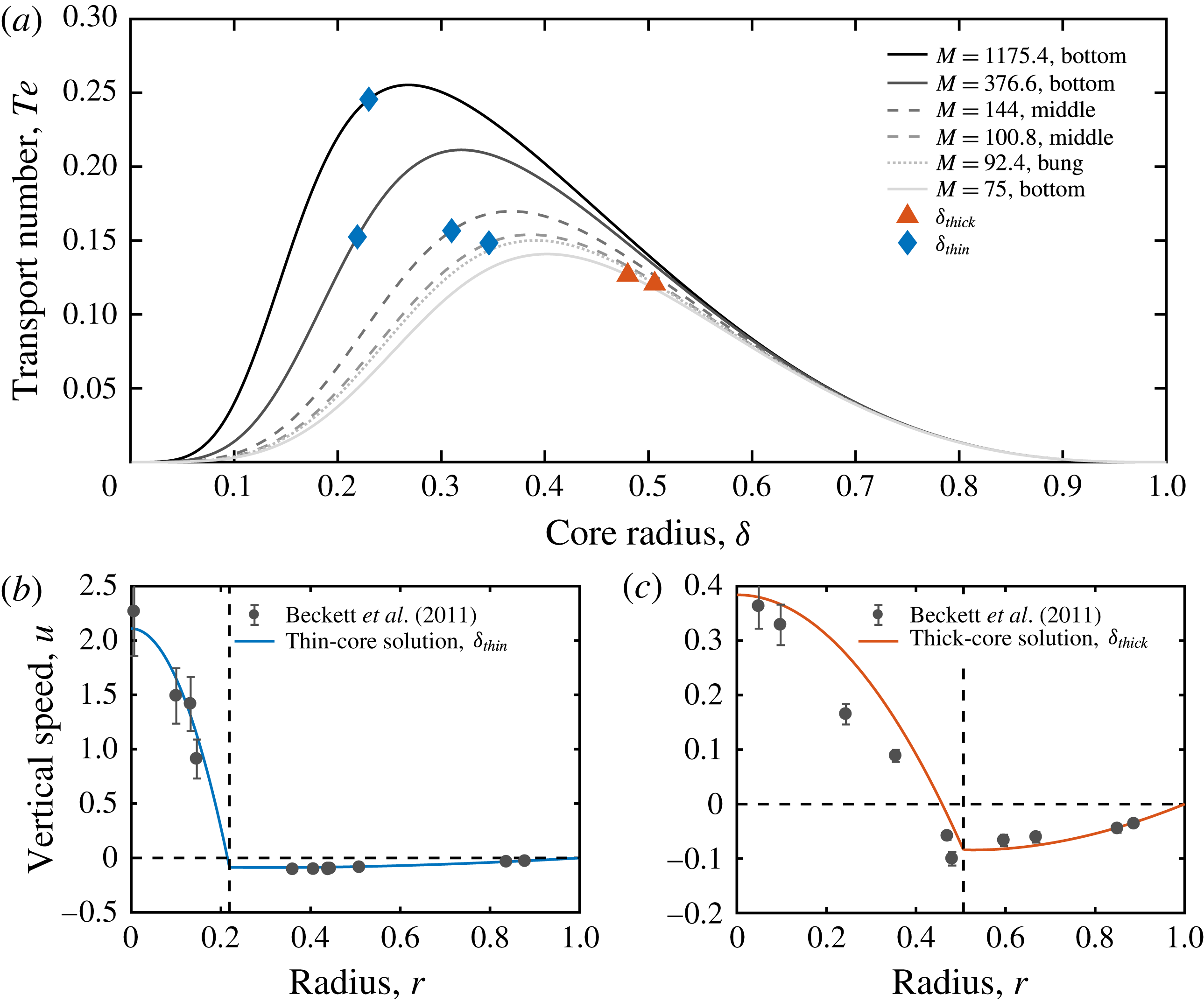
Comparison between the reproduction of experiment No. 5 (a) and an additional simulation with inverted viscosity contrast
 $1/M$
(b), where the heavy and now less viscous fluid (dark blue) forms a sinking core. (c) Horizontal speed profiles for the inverted (yellow line) and normal (red line) viscosity contrast case.
$1/M$
(b), where the heavy and now less viscous fluid (dark blue) forms a sinking core. (c) Horizontal speed profiles for the inverted (yellow line) and normal (red line) viscosity contrast case.
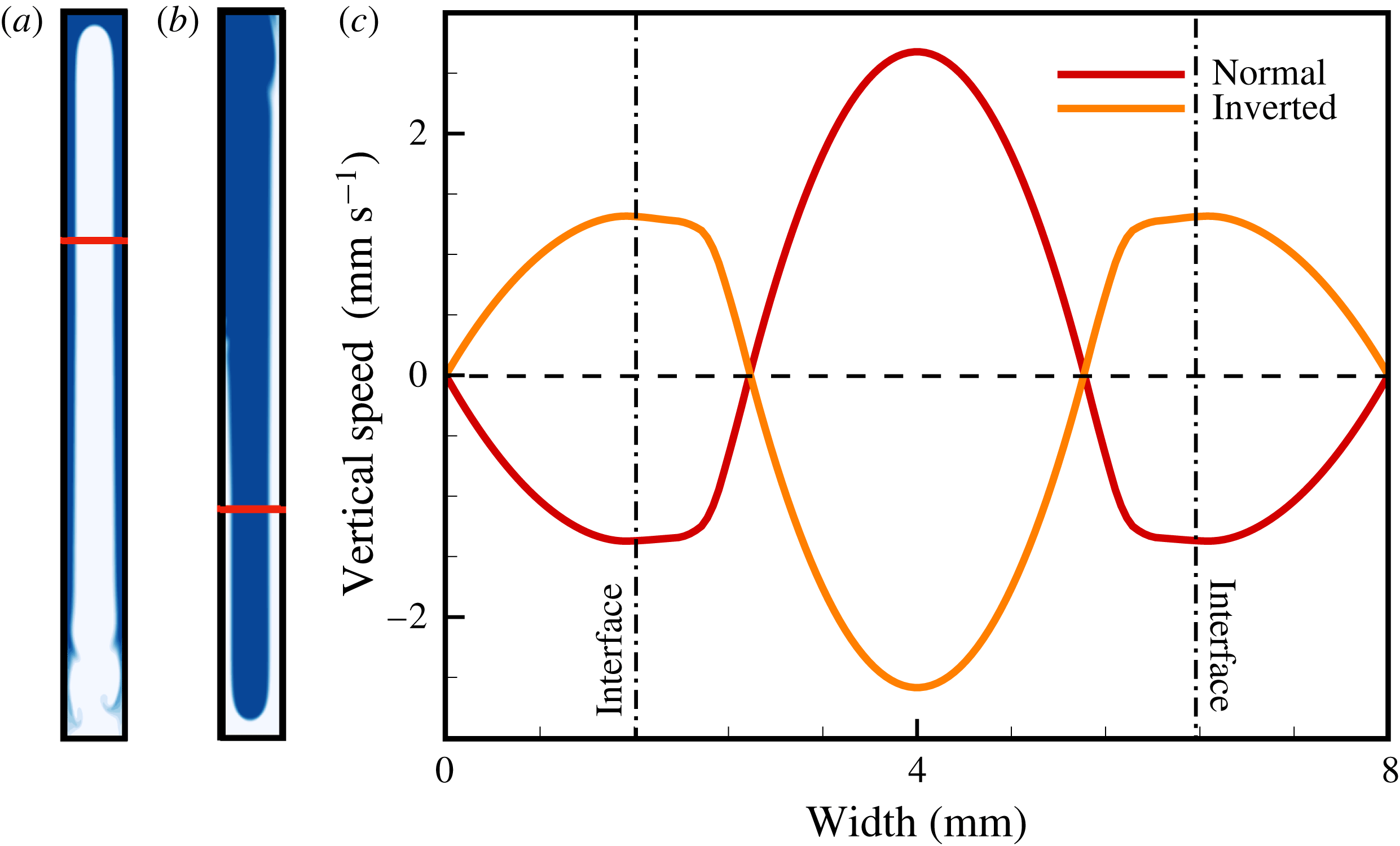
4.2 Ramifications for volcanic systems
In its current form, our model is not yet suitable for a direct quantitative comparison with field data from a specific volcano. Some of our insights, however, may inform the interpretation of field data on a conceptual level. One pertinent insight is that a change at either the base of a conduit or its opening in a volcanic crater could trigger a switch in the flow regime in the conduit. The effect of different flow regimes in the conduit on eruptive surface processes was well explored and reviewed by Vergniolle & Mangan (Reference Vergniolle and Mangan2000). Our results suggest that the reverse is possible as well: eruptive surface processes can alter the flow regime in the volcanic conduit. For example, a disruption at the free surface, which might arise during an eruption or other events such as mass movements in the crater, could trigger a switch in the flow configuration that is realized in the conduit. Of course, our simplistic boundary conditions (figure 11 d1–e3 and g1–h3) do not adequately represent eruptive processes at a free surface. Nonetheless, our results demonstrate the potentially significant role of surface conditions in selecting a flow regime in the conduit.
We argue that the existence of two different, stable flow configurations could be reflected in erupted field samples from persistently degassing volcanoes, potentially from different stages of the same eruption. A switch from thick- to thin-core flow could increase the magma ascent rate by more than an order of magnitude, which may be detectable in microanalytical data. Our results show that if a change in the estimated or measured ascent speed of the magma is detected, this observation does not necessarily require additional magma supply or a change in the volatile influx at depth. It could also be related to flow switching in the volcanic conduit.
Another potentially relevant insight of our study is the significant flow reversal present in all three of the flow regimes identified by Stevenson & Blake (Reference Stevenson and Blake1998). This result suggests that flow reversal might be the norm rather than the exception in volcanic conduits. Our analytical model predicts that flow reversal occurs in the less viscous phase, a finding that is corroborated by our simulations (see figure 13 and additional results in the supplementary material). Typically, the buoyant, volatile-rich magma has the lower viscosity, as was assumed in the experiment of Stevenson & Blake (Reference Stevenson and Blake1998). In that case, flow-reversal flux is oriented downward, which raises the question of whether the magma trapped in flow reversal is simply cycled back into a crustal reservoir never to be sampled by eruption, or whether some magma may circulate in the conduit for some time before being erupted. In the latter scenario, continued cycling along with mixing between different magma batches may lead to fundamentally different compositional evolution of both the magma and its volatile load than would be expected from a straight decompression path.
Flow reversal may also increase mixing between volatile-poor and volatile-rich magmatic melt, because the two fluids move in the same direction in some portion of the conduit. As demonstrated in figure 5(b,c), even a small amount of mixing could have important dynamic ramifications for conduit flow. As pointed out by Witham (Reference Witham2011), magma mixing during conduit convection could be relevant for understanding why observed melt-inclusion trends from persistently degassing volcanoes rarely coincide with modelled degassing trends, as recently reviewed in Métrich & Wallace (Reference Métrich and Wallace2008).
5 Conclusions
In this study, we reproduce, explain, and generalize laboratory experiments of buoyancy-driven exchange flow in vertical tubes. We derive an analytical model for core–annular flow – the most commonly observed configuration of bidirectional flow – that is consistent with laboratory observations and direct numerical simulations. The primary objective of this paper is to understand the variability of core–annular flow in the laboratory context, but our model may also provide a suitable starting point for integrating the additional complexity needed for quantifying conduit flow in persistently degassing volcanoes. The key finding of our analysis is that core–annular flow is bistable at finite viscosity contrast and that the pressure and fluxes at the boundaries of the domain, along with the transient history of the flow, play an important role in selecting the realized flow solution. This result implies that buoyancy-driven exchange flow is not uniquely determined by the material properties of the fluids and geometric parameters of the tube.
Author contributions
J.S. conceptualized the study, integrated the results from the numerical and the analytical model and wrote the paper. Z.Q. performed the numerical simulations and compiled the supplementary material. D.P. performed the analytical derivation and computations. T.K. assisted with the numerical modelling, creation of figures and the text. I.B. provided feedback on the study conception and the text.
Acknowledgements
The authors would like to thank F. Beckett for providing us with the laboratory data and two anonymous reviewers for helpful comments. E. Dunham and two anonymous reviewers provided insightful remarks that have helped improve this manuscript considerably. T.K. is grateful for support from the Swiss National Science Foundation’s Postdoc Mobility Fellowship no. P300P2_177816. The source code used in this study is available through GitLab at http://zapad.stanford.edu/sigma/JFM2018-bidirectional.
Supplementary material and movies
Supplementary material and movies are available at https://doi.org/10.1017/jfm.2018.382


 Open access