


1. Introduction
Thermally driven convective fluid motions are ubiquitous in various geophysical and astrophysical flows, and are important in many industrial applications. Rayleigh–Bénard convection (RBC) (Ahlers, Grossmann & Lohse Reference Ahlers, Grossmann and Lohse2009; Lohse & Xia Reference Lohse and Xia2010; Chillà & Schumacher Reference Chillà and Schumacher2012; Xia Reference Xia2013), where a fluid layer in a box is heated from below and cooled from above, and vertical convection (VC) (Ng et al. Reference Ng, Ooi, Lohse and Chung2015; Shishkina Reference Shishkina2016; Ng et al. Reference Ng, Ooi, Lohse and Chung2017, Reference Ng, Ooi, Lohse and Chung2018), where the fluid is confined between two differently heated isothermal vertical walls, have served as two classical model problems to study thermal convection. Vertical convection was also called convection in a differentially heated vertical box in many early papers (Paolucci & Chenoweth Reference Paolucci and Chenoweth1989; Le Quéré & Behnia Reference Le Quéré and Behnia1998). Both RBC and VC can be viewed as extreme cases of the more general so-called tilted convection (Guo et al. Reference Guo, Zhou, Cen, Qu, Lu, Sun and Shang2015; Shishkina & Horn Reference Shishkina and Horn2016; Wang et al. Reference Wang, Wan, Yan and Sun2018a,Reference Wang, Xia, Wang, Sun, Zhou and Wanb; Zwirner & Shishkina Reference Zwirner and Shishkina2018; Zwirner et al. Reference Zwirner, Khalilov, Kolesnichenko, Mamykin, Mandrykin, Pavlinov, Shestakov, Teimurazov, Frick and Shishkina2020; Zhang, Ding & Xia Reference Zhang, Ding and Xia2021), with a tilt angle of  $0^\circ$ for RBC and $90^\circ$ for VC. We focus on VC in this study. Vertical convection finds many applications in engineering, such as thermal insulation using double-pane windows or double walls, horizontal heat transport in water pools with heated/cooled sidewalls, crystal growth procedures, nuclear reactors, ventilation of rooms, and cooling of electronic devices, to name only a few. Vertical convection has also served as a model to study thermally driven atmospheric circulation (Hadley Reference Hadley1735; Lappa Reference Lappa2009) or thermally driven circulation in the ocean, e.g. next to an ice-block (Thorpe, Hutt & Soulsby Reference Thorpe, Hutt and Soulsby1969; Tanny & Tsinober Reference Tanny and Tsinober1988).
The main control parameters in VC are the Rayleigh number  $Ra\equiv g\alpha L^3\varDelta /(\nu \kappa )$ and the Prandtl number $Pr\equiv \nu /\kappa$. Here, $\alpha$, $\nu$ and $\kappa$ are the thermal expansion coefficient, the kinematic viscosity and the thermal diffusivity of the convecting fluid, respectively, $g$ is the gravitational acceleration, $\varDelta \equiv T_h-T_c$ is the temperature difference between the two side walls, and $L$ is the width of the convection cell. The aspect ratio $\varGamma \equiv H/L$ is defined as the ratio of height $H$ over width $L$ of the domain. The responses of the system are characterized by the Nusselt number $Nu\equiv {QL}/{(k\varDelta })$ and the Reynolds number $Re\equiv {UL}/{\nu }$, which indicate the non-dimensional heat transport and flow strength in the system, respectively. Here $Q$ is the heat flux crossing the system and $U$ is the characteristic velocity of the flow.
Since the pioneering work of Batchelor (Batchelor Reference Batchelor1954), who first addressed the case of steady-state heat transfer across double-glazed windows, VC has drawn significant attention especially in the 1980s and 1990s, and most of these studies used experiments or a two-dimensional (2-D) direct numerical simulation (DNS) in a square domain with unit aspect ratio. For relatively low  $Ra$ (e.g. $Ra < 10^3$), the flow is weak and heat is transferred mainly by thermal conduction. With increasing $Ra$, typical stratified flow structures appear in the bulk region (de Vahl Davis & Jones Reference de Vahl Davis and Jones1983), while the flow remains steady. With a further increase in $Ra$, the flow becomes unsteady with periodical/quasi-periodical or chaotic motions (Paolucci & Chenoweth Reference Paolucci and Chenoweth1989; Le Quéré & Behnia Reference Le Quéré and Behnia1998), and eventually becomes turbulent when $Ra$ is sufficiently high (Paolucci Reference Paolucci1990).
The onset of unsteadiness has been well explored in the past (Chenoweth & Paolucci Reference Chenoweth and Paolucci1986; Paolucci & Chenoweth Reference Paolucci and Chenoweth1989; Janssen & Henkes Reference Janssen and Henkes1995; Le Quéré & Behnia Reference Le Quéré and Behnia1998). Paolucci & Chenoweth (Reference Paolucci and Chenoweth1989) investigated the influence of the aspect ratio  $\varGamma$ on the onset of unsteadiness for 2-D VC with $Pr=0.71$. They found that for $\varGamma \gtrsim 3$, the first transition from the steady state arises from an instability of the sidewall boundary layers, while for smaller aspect ratios $0.5\le \varGamma \lesssim 3$, it arises from internal waves near the departing corners. Such oscillatory instability arising from internal waves was first reported by Chenoweth & Paolucci (Reference Chenoweth and Paolucci1986). Paolucci & Chenoweth (Reference Paolucci and Chenoweth1989) also found that for $\varGamma =1$, the critical Rayleigh number $Ra_c$ for the onset of unsteadiness lies between $1.8\times 10^{8}$ and $2\times 10^8$. Later work, with $Pr=0.71$ and $\varGamma =1$ by Le Quéré & Behnia (Reference Le Quéré and Behnia1998), also showed that the internal gravity waves play an important role in the time-dependent dynamics of the solutions, and $1.81\times 10^8\le Ra_c\le 1.83\times 10^8$ was determined to be the range of the critical Rayleigh number. Janssen & Henkes (Reference Janssen and Henkes1995) studied the influence of $Pr$ on the instability mechanisms for $\varGamma =1$, and observed that for $0.25\le Pr\le 2$, the transition occurs through periodic and quasi-periodic flow regimes. One bifurcation is related to an instability occurring in a jet-like fluid layer exiting from the corners of the cavity where the vertical boundary layers are turned horizontal. Such jet-like flow structures are responsible for the generation of internal gravity waves (Chenoweth & Paolucci Reference Chenoweth and Paolucci1986; Paolucci & Chenoweth Reference Paolucci and Chenoweth1989). The other bifurcation occurs in the boundary layers along the vertical walls. Both of these instabilities are mainly shear-driven. For $2.5\le Pr\le 7$, Janssen & Henkes (Reference Janssen and Henkes1995) found an ‘immediate’ (i.e. sharp) transition from the steady to the chaotic flow regime, without intermediate regimes. This transition is also caused by boundary layer instabilities. They also showed that $Ra_c$ significantly increases with increasing $Pr$, e.g. for $Pr=4$, the flow can still be steady with $Ra=2.5\times 10^{10}$. However, owing to the computation limit, unsteady motions for the large- $Pr$ cases have largely remained unexplored in the past.
Additionally, the flow structures for VC have been examined in detail. A typical flow feature for VC is the stably-stratified bulk region (de Vahl Davis & Jones Reference de Vahl Davis and Jones1983; Ravi, Henkes & Hoogendoorn Reference Ravi, Henkes and Hoogendoorn1994; Trias et al. Reference Trias, Soria, Oliva and Pérez-Segarra2007; Sebilleau et al. Reference Sebilleau, Issa, Lardeau and Walker2018; Chong et al. Reference Chong, Yang, Wang, Verzicco and Lohse2020). Such stratification can be quantified by the time-averaged non-dimensional temperature gradient at the centre, namely
 \begin{equation} S\equiv\left\langle (L/\varDelta)(\partial{T}/\partial{z})_c\right\rangle_t. \end{equation}
Here  $\left \langle \right \rangle _t$ denotes a time average. Gill (Reference Gill1966) derived asymptotic solutions for high $Pr$, and predicted $S=0.42$ as $Ra\to \infty$, while an accurate solution of the same system by Blythe, Daniels & Simpkins (Reference Blythe, Daniels and Simpkins1983) predicted a value of 0.52. Later DNS results for $Ra=10^8$ and $Pr=70$ yielded $S=0.52$ (Ravi et al. Reference Ravi, Henkes and Hoogendoorn1994), which is in excellent agreement with the theoretical prediction by Blythe et al. (Reference Blythe, Daniels and Simpkins1983). However, for small $Pr$, the structure of the core and the vertical boundary layer are no longer similar to those predicted by the asymptotic solutions which are valid for large $Pr$ (Blythe et al. Reference Blythe, Daniels and Simpkins1983). Unfortunately, there exists no such asymptotic theory for finite $Pr$. Only Graebel (Reference Graebel1981) has presented some approximate solutions, in which some terms have been neglected in the equations. For $Pr=0.71$, his prediction yielded $S=0.49$, which is considerably smaller than the value $S\approx 1$ from DNS (Ravi et al. Reference Ravi, Henkes and Hoogendoorn1994; Trias et al. Reference Trias, Soria, Oliva and Pérez-Segarra2007). It was concluded that $S$ is independent of $Ra$ for $Ra\le 10^{10}$ (Paolucci Reference Paolucci1990); however, it is evident that the dependence of $S$ on $Ra$ and $Pr$, especially for those with high $Ra>10^{10}$ and low $Pr<0.71$, is still poorly understood.
A key question in the study of thermal convection is: How do  $Nu$ and $Re$ depend on $Ra$ and $Pr$? This question has been extensively addressed in RBC over the past years (Ahlers et al. Reference Ahlers, Grossmann and Lohse2009). For RBC, the mean kinetic dissipation rate ( $\epsilon _u$) and thermal dissipation rate ( $\epsilon _\theta$) obey exact global balances, which feature $Ra$,
$Ra$,  $Nu$ and $Pr$ (Shraiman & Siggia Reference Shraiman and Siggia1990). For this problem, in a series of papers, Grossmann & Lohse (Reference Grossmann and Lohse2000, Reference Grossmann and Lohse2001, Reference Grossmann and Lohse2002, Reference Grossmann and Lohse2004) developed a unifying theory to account for $Nu(Ra,Pr)$ and $Re(Ra,Pr)$ over wide parameter ranges. The central idea of the theory is a decomposition of $\epsilon _u$ and $\epsilon _\theta$ into their boundary layer and bulk contributions. The theory has been well confirmed through various experiments and numerical simulations (Stevens et al. Reference Stevens, van der Poel, Grossmann and Lohse2013). This theory has also been applied to horizontal convection (Shishkina, Grossmann & Lohse Reference Shishkina, Grossmann and Lohse2016; Shishkina & Wagner Reference Shishkina and Wagner2016) and internally heated convection (Wang, Shishkina & Lohse Reference Wang, Shishkina and Lohse2020b). However, in VC, the exact relation for $\epsilon _u$ does not hold, which impedes the applicability of the unifying theory to the scalings in VC (Ng et al. Reference Ng, Ooi, Lohse and Chung2015).
As compared with RBC, for VC, much less work has been devoted to the dependences  $Nu(Ra,Pr)$ and $Re(Ra,Pr)$. Past studies have suggested power law dependences, i.e. $Nu\sim Ra^\beta$ and $Re\sim Ra^\gamma$, at least in a certain $Ra$ range. The reported scaling exponent $\beta$ was found to vary from 1/4 to 1/3 (Xin & Le Quéré Reference Xin and Le Quéré1995; Le Quéré & Behnia Reference Le Quéré and Behnia1998; Trias et al. Reference Trias, Soria, Oliva and Pérez-Segarra2007, Reference Trias, Gorobets, Soria and Oliva2010; Ng et al. Reference Ng, Ooi, Lohse and Chung2015; Shishkina Reference Shishkina2016; Wang et al. Reference Wang, Xia, Yan, Sun and Wan2019; Ng et al. Reference Ng, Spandan, Verzicco and Lohse2020), depending on the $Ra$ range and $Pr$. Ng et al. (Reference Ng, Ooi, Lohse and Chung2015) simulated three-dimensional (3-D) VC with periodic conditions in the range $10^5\le Ra\le 10^9$ with $Pr=0.709$, and obtained $\beta =0.31$ as the considered range. For much larger $Pr\gg 1$ and using laminar boundary layer theories, Shishkina (Reference Shishkina2016) theoretically derived $Nu\sim Ra^{1/4}$ and $Re\sim Ra^{1/2}$. These theoretical results are in excellent agreement with direct numerical simulations for $Ra$ from $10^5$ to $10^{10}$ in a cylindrical container with aspect ratio $\varGamma =1$. The power law exponents $\beta =1/4$ and $\gamma =1/2$ were also confirmed by the DNS of Ng et al. (Reference Ng, Spandan, Verzicco and Lohse2020) in a 3-D cell with span-wise periodic boundary conditions for $10^8\le Ra\le 1.3\times 10^9$. For 2-D VC, past studies with $Ra\le 10^{10}$ have also shown that $\beta$ is closer to 1/4 than 1/3 (Xin & Le Quéré Reference Xin and Le Quéré1995; Trias et al. Reference Trias, Soria, Oliva and Pérez-Segarra2007, Reference Trias, Gorobets, Soria and Oliva2010; Wang et al. Reference Wang, Xia, Yan, Sun and Wan2019). Wang et al. (Reference Wang, Xia, Yan, Sun and Wan2019) simulated 2-D VC over $10^5\le Ra\le 10^9$ for fixed $Pr=0.71$, and found $\beta \approx 0.27$ and $\gamma \approx 0.50$.
Most of the simulations for VC were conducted for  $Ra\lesssim 10^{10}$. The high- $Ra$ simulations become stiff owing to a decrease in the boundary-layer thicknesses with increasing $Ra$. As a result, little is known about what will happen at $Ra$ much larger than $10^{10}$. In this study, we attempt to fill this gap in knowledge by performing DNS up to $Ra=10^{14}$. The price we have to pay is that for such large $Ra$, we are restricted to 2-D.
The main questions we want to address in this study are as follows.
(i) Is the conclusion that $S$ is independent of $Ra$ for $Ra\le 10^{10}$ (Paolucci Reference Paolucci1990) still valid for $Ra$ much larger than $10^{10}$?
(ii) How does the global flow organization (mean temperature and velocity profiles) change with increasing
$Ra$ up to $10^{14}$?(iii) How robust are the laminar scaling relations
$Nu\sim Ra^{1/4}$ and $Re\sim Ra^{1/2}$ (Shishkina Reference Shishkina2016) for higher $Ra$? Will new scaling relations appear for $Ra$ much larger than $10^{10}$?


We find that  $S$ is not independent of $Ra$ over the studied parameter range at all. Instead, we find that apart from the small- $Ra$ regime (now called regime I), where $S$ only weakly depends on $Ra$ (Paolucci Reference Paolucci1990), there are additional regimes for $Ra\gtrsim 5\times 10^{10}$ with different scaling relations. In regime II ( $5\times 10^{10} \lesssim Ra \lesssim 10^{13}$), with increasing $Ra$,
$Ra$,  $S$ first increases (regime $\textrm {{II}}_a$) to its maximum and then decreases (regime $\textrm {{II}}_b$) again. In regime III ( $Ra\gtrsim 10^{13}$), $S$ again becomes weakly dependent on $Ra$, with a smaller value than that of regime I. Furthermore, we find that the laminar power law exponents $\beta =1/4$ and $\gamma =1/2$ undergo sharp transitions to $\beta \approx 1/3$ and $\gamma \approx 4/9$ when $Ra\gtrsim 5\times 10^{10}$, i.e. at the transition from regime I to regime II.
The rest of the paper is organized as follows. Section 2 describes the governing equations and numerical methods. The different flow organizations in the different regimes are studied in § 3. In § 4, we discuss the transition of the scaling relations for heat and momentum transport between the different regimes. Finally, § 5 contains a summary and an outlook.
2. Numerical procedures
A sketch of 2-D VC is shown in figure 1. The top and bottom walls are insulated. The left wall is heated with temperature  $T_h$, while the right wall is cooled with temperature $T_c$. No-slip and no-penetration velocity boundary conditions are used at all the walls. The aspect ratio $\varGamma \equiv H/L$ is fixed to 1. The dimensionless governing equations are the incompressible Navier–Stokes equations with an Oberbeck–Boussinesq approximation:
 \begin{gather} \boldsymbol{\nabla}\boldsymbol{\cdot}\boldsymbol{u} = 0, \end{gather}
 \begin{gather}\frac{\partial \boldsymbol{u}}{\partial t} + \boldsymbol{u}\boldsymbol{\cdot}\boldsymbol{\nabla}\boldsymbol{u} ={-}\boldsymbol{\nabla} p+ \sqrt{\frac{Pr}{Ra}}\nabla^2\boldsymbol{u} + \theta{\boldsymbol{\boldsymbol{e}}_z}, \end{gather}
 \begin{gather}\frac{\partial \theta}{\partial t} + \boldsymbol{u}\boldsymbol{\cdot} \boldsymbol{\nabla} \theta =\frac{1}{\sqrt{RaPr}}\nabla^2\theta. \end{gather}
Here  $\boldsymbol {\boldsymbol {e}}_z$ is the unit vector pointing in the direction opposite to gravity. The dimensionless velocity, temperature and pressure are represented by $\boldsymbol {u}\equiv {(u,w)}$, $\theta$ and $p$, respectively. For non-dimensionalization, we use the width of the convection cell $L$ and the free-fall velocity $U={(g\alpha {\rm \Delta} L)}^{1/2}$. Temperature is non-dimensionalized as $\theta =(T-T_c)/\varDelta$.
Sketch of two-dimensional vertical convection with unit aspect ratio. The left vertical wall is heated ( $T=T_h$), while the right vertical wall is cooled ( $T=T_c$), and the temperature difference is $\varDelta =T_h-T_c$. The top and bottom walls are adiabatic. All the walls have no-slip and no-penetration velocity boundary conditions.

The governing equations were solved using the second-order staggered finite-difference code AFiD (Verzicco & Orlandi Reference Verzicco and Orlandi1996; van der Poel et al. Reference van der Poel, Ostilla-Mónico, Donners and Verzicco2015). The code has already been extensively used to study RBC (Wang et al. Reference Wang, Chong, Stevens, Verzicco and Lohse2020a,Reference Wang, Verzicco, Lohse and Shishkinac; Liu et al. Reference Liu, Chong, Wang, Ng, Verzicco and Lohse2021) and internally heated convection (Wang et al. Reference Wang, Shishkina and Lohse2020b). Direct numerical simulation was performed for  $10^7\le Ra\le 10^{14}$ with a fixed $Pr=10$. Stretched grids were used to resolve the thin boundary layers and adequate resolutions were ensured to resolve the small scales of turbulence (Shishkina et al. Reference Shishkina, Stevens, Grossmann and Lohse2010). Grids with up to $8192\times 8192$ nodes were used for the highest $Ra=10^{14}$. We performed careful grid independence checks for several high- $Ra$ cases. It was found that the difference of $Nu$ and $Re$ for the different grids were always smaller than $1\,\%$ and $2\,\%$, respectively. Details on the simulations are provided in table 2 in the appendix.
3. Global flow organization
3.1. Global flow fields
We first focus on the change of global flow organizations with increasing  $Ra$. Figure 2 shows instantaneous temperature, horizontal velocity ( $u$) and vertical velocity ( $w$) fields for different $Ra$. For the considered $Pr=10$, we find that the flow is still steady for $Ra=5\times 10^{10}$, as shown in figure 2(a–c), which is consistent with the finding that the critical Rayleigh number $Ra_c$ for the onset of unsteadiness increases with increasing $Pr$ and that the flow is indeed still steady for $Ra=2.5\times 10^{10}$ with $Pr=4$ (Janssen & Henkes Reference Janssen and Henkes1995). This is in sharp contrast with RBC, where the flow is already turbulent for such high $Ra$ with $Pr=10$ (Wang et al. Reference Wang, Verzicco, Lohse and Shishkina2020c). The flow is stably stratified in the bulk region, as shown in figure 2(a). The large horizontal velocity regions mainly concentrate near the top and bottom walls (figure 2b), while the strong vertical motion mainly occurs near the two sidewalls (figure 2c). Such flow structures are typical for steady VC with large $Pr$ (Ravi et al. Reference Ravi, Henkes and Hoogendoorn1994).
Instantaneous temperature  $\theta$ (a,d,g,j), horizontal velocity $u$ (b,e,h,k) and vertical velocity (c,f,i,l) fields for different $Ra$ with $Pr=10$ and $\varGamma =1$. (a–c) Regime I where $Ra=5\times 10^{10}$. (d–f) Regime II where $Ra=6\times 10^{10}$. (g–i) Regime II where $Ra=6\times 10^{11}$. (j–l) Regime III where $Ra=10^{14}$. The arrows in (a) indicate the velocity directions.

However, with a minor increase of  $Ra$ from $Ra=5\times 10^{10}$ to $Ra=6\times 10^{10}$, the flow becomes instantaneously chaotic, as shown in figure 2(d–f). This finding is consistent with the previous result that for $Pr\ge 2.5$, there is an immediate transition from the steady to the chaotic flow regime without intermediate regimes (Janssen & Henkes Reference Janssen and Henkes1995). This transition is caused by boundary layer instabilities, which are reflected in the plume ejections in the downstream of the boundary layers (figure 2d). The strong horizontal/vertical fluid motions still concentrate near the horizontal/vertical walls, as indicated in figures 2(e) and 2(f). However, there are already some chaotic features appearing in the bulk, which suggest a change of the bulk properties.
When  $Ra$ is further increased to $6\times 10^{11}$ (figure 2g–i), further evident changes of the global flow organization appear as follows. (i) The hot plumes mainly eject over the upper half of the hot sidewall, and enter the upper half of the bulk region. This makes the hot upper bulk region more isothermal than in the smaller- $Ra$ cases. Similar processes happen for the cold plumes and the lower cold bulk region. Therefore, figure 2(g) clearly shows a larger centre temperature gradient than those in figures 2(a) and 2(d). (ii) The strong horizontal motions now not only occur near the horizontal walls, but also in the bulk region (figure 2h), and alternating rightward and leftward ‘zonal flow’ structures appear.
For the highest  $Ra=10^{14}$ (figure 2j–l), the thermal driving is so strong that hot plumes are now ejected over large fractions of the left vertical wall ( $0.2 \lesssim z/L \lesssim 1$). The plumes are transported into the bulk region by the zonal flow structures shown in figure 2(k). This process causes efficient mixing in the bulk, which then leads to a smaller centre temperature gradient. Further prominent features are the ‘layered’ structures near the top and bottom walls, where relatively hot/cold fluids clearly separate from the near-isothermal bulk region.
3.2. Mean profiles for temperature and horizontal velocity
We have seen that the global flow organization evidently changes with increasing  $Ra$. In this subsection, we quantify these changes by looking at the mean profiles for the temperature and for the horizontal velocity. Figure 3(a) clearly shows the change in the temperature profiles at $x/L=0.5$ with increasing $Ra$, which is consistent with the temperature fields presented in figure 2. The change of the bulk temperature profile shape can be quantified by the time-averaged non-dimensional vertical temperature gradient in the cell centre, i.e. $S\equiv \left \langle (L/\varDelta )(\partial {T}/\partial {z})_c\right \rangle _t$ (Paolucci Reference Paolucci1990; Ravi et al. Reference Ravi, Henkes and Hoogendoorn1994). This quantity is plotted in figure 3(b), where one can observe three different regimes. In the well-explored regime I ( $Ra \lesssim 5\times 10^{10}$), $S$ weakly depends on $Ra$, with a value $S\approx 0.5$, close to that of $S=0.52$ for $Ra=10^8$ with $Pr=70$ reported in Ravi et al. (Reference Ravi, Henkes and Hoogendoorn1994). However, in regime II ( $5\times 10^{10} \lesssim Ra \lesssim 10^{13}$), $S$ has a non-monotonic dependence on $Ra$: it first increases with increasing $Ra$, reaches its maximum at $Ra=6\times 10^{11}$, and then decreases again. Regime II is further divided into regime $\textrm {{II}}_a$, where $S$ increases with increasing $Ra$, and regime $\textrm {{II}}_b$, where $S$ decreases with increasing $Ra$. The onset of regime II coincides with the onset of unsteadiness, which shows that plume emissions play an important role in altering the bulk properties. The maximum of $S$ occurs when approximately half of sidewall areas (downstream) feature plume emissions, as shown in figure 2(g). Finally, in regime III, $S$ again becomes weakly dependent on $Ra$, while it has a smaller value than that of regime I. The small value of $S$ in regime III arises from the well-mixed bulk region, as can be seen in figure 2(j).
(a) Mean temperature profiles  $\theta (z)$ at $x/L=0.5$ for different $Ra$ with $Pr=10$. (b) Time-averaged centre vertical temperature gradient $S=\left \langle (L/\varDelta )(\partial {T}/\partial {z})_c\right \rangle _t$ as a function of $Ra$ for $Pr=10$. In regime I and regime III, $S$ is weakly dependent on $Ra$. In contrast, in regime II, $S$ displays a non-monotonic dependence on $Ra$. Regime II is further divided into $\textrm {{II}}_a$ and $\textrm {{II}}_b$, in which $S$ increases or decreases with increasing $Ra$, respectively. (c) Mean horizontal velocity profiles at $x/L=0.5$ for different $Ra$ with $Pr=10$. Panels (a) and (c) share the same legend.

Figure 3(c) shows the change of the horizontal velocity profiles with increasing  $Ra$. In regime I, the strong horizontal fluid motions concentrate near the top and bottom walls. In contrast, in regime III, the largest horizontal velocity appears in the bulk region, and alternating rightward and leftward fluid motions, i.e. zonal flows, are observed even after time averaging, which is consistent with the instantaneous horizontal velocity field shown in figure 2(k). Another prominent flow feature of regime III is that the horizontal velocity near the top and bottom walls is close to 0. This means that the ‘layered structure’ near the top and bottom walls, as indicated in the temperature field in figure 2(j), is actually nearly a ‘dead zone’ with weak fluid motions. Thus the appearance of this nearly ‘dead’ layered structure indicates the the onset of regime III. Regime II serves to connect regime I and regime III: in regime $\textrm {{II}}_a$, the strongest horizontal motion still takes place near the top and bottom walls, see, e.g. the horizontal velocity profile for $Ra=2\times 10^{11}$ in figure 3(c). In contrast, in regime $\textrm {{II}}_b$, the strongest horizontal fluid motions appear in the bulk, see, e.g. the strong zonal flow motions in the central region for $Ra=10^{12}$, as shown in figure 3(c). We remark that the zonal flow has been found in many geo- and astrophysical flows (Yano, Talagrand & Drossart Reference Yano, Talagrand and Drossart2003; Heimpel, Aurnou & Wicht Reference Heimpel, Aurnou and Wicht2005; Nadiga Reference Nadiga2006), and it has also been extensively studied in RBC (Goluskin et al. Reference Goluskin, Johnston, Flierl and Spiegel2014; Wang et al. Reference Wang, Chong, Stevens, Verzicco and Lohse2020a; Zhang et al. Reference Zhang, Van Gils, Horn, Wedi, Zwirner, Ahlers, Ecke, Weiss, Bodenschatz and Shishkina2020; Reiter et al. Reference Reiter, Zhang, Stepanov and Shishkina2021). It is remarkable and interesting to also observe zonal flows in the high- $Ra$ VC system. This system thus provides another model to study the physics of the zonal flow.
3.3. Mean profiles for temperature and vertical velocity
We now consider the mean vertical velocity and temperature profiles in the longitudinal ( $x$) direction. Figure 4(a) shows the mean temperature profiles in the longitudinal ( $x$) direction at mid-height $z/L=0.5$ for different $Ra$. It is seen that for $Ra$ values that are not too high, the temperature does not monotonically drop from $\theta =1$ at the hot wall to $\theta =0.5$ in the core. Instead, an undershoot phenomenon is observed. This phenomenon arises from the stable stratification in the bulk (Ravi et al. Reference Ravi, Henkes and Hoogendoorn1994) and can also be observed in the similarity solutions of the boundary layer equations for natural convection over a vertical hot wall in a stably stratified environment (Henkes & Hoogendoorn Reference Henkes and Hoogendoorn1989). However, for $Ra\ge 10^{12}$, we find that the overshoot phenomenon disappears. This arises from the continuous emissions of hot plumes at mid-height $z/L=0.5$ and beyond, as then the hot fluid directly touches the well-mixed bulk flow with small stratification.
Mean (a) longitudinal temperature profile and (b) longitudinal profile of the vertical velocity at mid-height  $z/L=0.5$ for different $Ra$ with $Pr=10$. Panels (a) and (b) share the same legend.

Figure 4(b) shows vertical velocity profiles in the longitudinal direction, again at mid-height  $z/L=0.5$. With increasing $Ra$, the boundary layer becomes thinner and the peak vertical velocity becomes smaller. This finding reflects the different flow organizations in the different regimes: the emitted plumes in regimes II and III weaken the overall vertical fluid motions, as compared with the steady flow organization in regime I. This is also reflected in the $Re\sim Ra^\gamma$ scaling, as will be discussed below.
4. Global heat and momentum transport and dissipation rates
Next, we focus on the global heat ( $Nu$) and momentum ( $Re$) transport. Here, we use the wind-based Reynolds number $Re$ with the characteristic velocity
 \begin{equation} U_{max} \equiv \operatorname*{max}_{x}H^{{-}1}\int_{0}^{H}w\,\textrm{d} z, \end{equation}
which is the same definition as that in Shishkina (Reference Shishkina2016), and the root-mean-square Reynolds number  $Re_{rms}$ with the characteristic velocity
 \begin{equation} U_{rms}\equiv\sqrt{\left\langle \boldsymbol{u}\boldsymbol{\cdot}\boldsymbol{u}\right\rangle_{V,t}}, \end{equation}
where  $\left \langle \right \rangle _{V,t}$ indicates volume and time averaging. Figures 5(a) and 5(b) show that in regime I, the obtained effective power law scaling relations agree remarkably well with the theoretical prediction made for laminar VC (Shishkina Reference Shishkina2016), namely, $Nu\sim Ra^{1/4}$ and $Re\sim Ra^{1/2}$. The fitted scaling relations are provided in table 1. It is also seen that a slightly faster growth of $Nu$ with $Ra$ is obtained for $Ra\le 10^{9}$. A similar increase of the scaling exponent for small $Ra$ has also been found previously in both confined (Shishkina Reference Shishkina2016; Wang, Zhang & Guo Reference Wang, Zhang and Guo2017; Wang et al. Reference Wang, Xia, Yan, Sun and Wan2019) and double periodic VC (Ng et al. Reference Ng, Ooi, Lohse and Chung2015). However, when $Ra\ge 5\times 10^{10}$, in regime II and regime III, evidently different scaling relations are observed. The fitted power law scaling relations (see table 1 for the obtained values) are close to $Nu\sim Ra^{1/3}$ (referred to as Malkus scaling Malkus Reference Malkus1954) and $Re\sim Ra^{4/9}$, which, interestingly, were predicted for regime $\textrm {{IV}}_u$ by the unifying theory for RBC (Grossmann & Lohse Reference Grossmann and Lohse2000). Such observation of scaling transitions further demonstrates that there are no pure scaling laws in thermal convection. This has already been seen in RBC (Grossmann & Lohse Reference Grossmann and Lohse2000; Ahlers et al. Reference Ahlers, Grossmann and Lohse2009), horizontal convection (Shishkina et al. Reference Shishkina, Grossmann and Lohse2016; Shishkina & Wagner Reference Shishkina and Wagner2016; Reiter & Shishkina Reference Reiter and Shishkina2020) and internally heated convection (Wang et al. Reference Wang, Shishkina and Lohse2020b), and apparently crossovers between different scaling regimes also occur here. However, the sharpness of the scaling transition from $\beta =1/4$ to $\beta =1/3$ observed here is quite different from the smooth transition seen in RBC. Indeed, in RBC, the transition from $Nu\sim Ra^{1/4}$ to $Nu\sim Ra^{1/3}$ is very smooth, spread over more than two orders of magnitude in $Ra$ (Grossmann & Lohse Reference Grossmann and Lohse2000), and the linear combination of the $1/4$ and $1/3$ power laws even mimics an effective $2/7$ scaling exponent (Castaing et al. Reference Castaing, Gunaratne, Heslot, Kadanoff, Libchaber, Thomae, Wu, Zaleski and Zanetti1989) over many orders of magnitude in $Ra$.
$Ra$.
(a) Normalized Nusselt number  $Nu/Ra^{1/4}$, (b) normalized Reynolds number based on maximal vertical velocity $Re/Ra^{1/2}$, and (c) normalized Reynolds number based on root-mean-square velocity $Re_{rms}/Ra^{1/2}$, as functions of $Ra$ for $Pr=10$. The solid lines connect the DNS data points, whereas the dashed lines show the suggested scaling laws. There is a clear and sharp transition in scaling between regime I and regime II/III.

Fitted scaling relations of the Nusselt number  $Nu$, the Reynolds number based on maximal vertical velocity $Re$ (4.1), the Reynolds number based on root-mean-square velocity $Re_{rms}$ (4.2) and the normalized kinetic dissipation rate $\left \langle \epsilon _u\right \rangle /[L^{-4}\nu ^{3}(Nu-1)RaPr^{-2}]$ with respect to $Ra$ for the three different regimes.

Figure 5(c) shows that also  $Re_{rms}$ behaves differently in different regimes. The fitted scaling relation $Re_{rms}\sim Ra^{0.37}$ in regime I is the same as that found for 2-D VC with $Pr=0.71$ (Wang et al. Reference Wang, Xia, Yan, Sun and Wan2019), which suggests that in vertical convection, different Reynolds numbers have different scaling relations with $Ra$. In regime II, the normalized Reynolds number $Re_{rms}/Ra^{1/2}$ depends non-monotonically on $Ra$, and shows a pronounced local minimum. The fitted scaling exponent 0.31 in regime III is again smaller than that in regime I.
It is interesting to note that, though  $S$ shows a clear transition between regime II and regime III, this transition is not seen in the effective power law scaling relations $Nu\sim Ra^\beta$ and $Re\sim Ra^\gamma$. Our interpretation of this noteworthy finding is as follows. The transition of the flow organization from regime I to regime II is sharp in view of the sudden appearance of plume emissions from the sidewall thermal boundary layers, and in view of the emergence of the local minimum of the Nusselt number distribution on the sidewall. However, the transition of flow organization from regime II to regime III is more continuous. The flows in these two regimes are characterized by the alternating rightward and leftward fluid motions, i.e. zonal flows, in the bulk, and they all have plume emissions from the sidewall boundary layers and a local minimum of the Nusselt number distribution on the sidewall. The only prominent difference is the appearance of layered structures near the top and bottom plates in regime III. As this layered structure only concentrates in a small region near the top and bottom plates, the global effective scaling exponents of Nu and Re do not seem to be sensitive to the different flow organizations in regimes II and III.
To better understand the sudden change of the global heat transport properties at the transition to regime II, we now consider the wall heat flux, which is denoted by the local Nusselt number at the wall  $Nu(z)|_{x=0,1}=\partial \left \langle \theta \right \rangle _t/\partial x|_{x=0,1}$. Figure 6(a) displays $Nu(z)|_{x=0}$ at the left wall, while $Nu(z)|_{x=1}$ at the right wall is not shown owing to the inherent symmetry of the system. For $Ra\le 5\times 10^{10}$, the local $Nu(z)|_{x=0}$ generally decreases monotonically with increasing heights $z$. The large local $Nu(z)|_{x=0}$ for small heights $z$ is attributed to the fact that the hot fluid there is in direct contact with the cold fluid, which leads to large temperature gradients. In contrast, for $Ra>5\times 10^{10}$, a local minimum and a local maximum in $Nu(z)|_{x=0}$ are identified, the heights of which are denoted as $z_{t1}$ and $z_{t2}$. It is clearly seen that $Nu(z)|_{x=0}$ after the first transition point $z_{t1}$ increases compared with the steady cases at $Ra \le 5\times 10^{10}$. This is because the emissions of the plumes lead to more efficient shear-driven mixing, and therefore larger local $Nu(z)|_{x=0}$. Thus, the overall heat transport also increases in regime II and later regime III (figure 5a) owing the ejections of plumes, and the change of the scaling is also related to the change of the boundary layer properties.
(a) Local Nusselt number  $Nu(z)$ at the hot wall ( $x/L=0$) for different $Ra$, all with $Pr=10$. (b) Transition points $z_t/L$ as functions of $Ra$. Here, $z_{t1}$ and $z_{t2}$ are the locations where $Nu(z)$ reaches its local minimum and maximum values, respectively. Such local maximum and minimum occur beyond $Ra\gtrsim 5\times 10^{10}$, see (a). The dashed vertical line denotes the $Ra$ where the centre temperature gradient is maximal.

We have shown that the two transition points  $z_{t1}$ and $z_{t2}$ roughly correspond to the locations where plumes begin to be ejected. Figure 6(b) shows, as expected, that both $z_{t1}$ and $z_{t2}$ decrease with increasing $Ra$, which suggests that the locations where hot plumes begin to be ejected move downwards with increasing $Ra$. At $Ra=6\times 10^{11}$, where the centre temperature gradient $S$ achieves its maximum, it can be seen that the mid-height $z/L=0.5$ lies between the two transition points, further demonstrating that the maximum of $S$ is achieved once plumes are ejected over approximately half of the area (downstream) of the sidewalls, as seen in the temperature field in figure 2(g).
Finally, we discuss the thermal and kinetic dissipation rates. In RBC, the following exact relations hold (Shraiman & Siggia Reference Shraiman and Siggia1990).
 \begin{gather} \left\langle \epsilon_u\right\rangle_{V}=\frac{\nu^3}{L^4}(Nu-1)RaPr^{{-}2}, \end{gather}
 \begin{gather}\left\langle \epsilon_\theta\right\rangle_{V}=\kappa\frac{\varDelta^2}{L^2}Nu. \end{gather}
The average  $\left \langle \right \rangle _V$ is over the whole volume and over time. In VC, the relation (4.4) still holds, however, the relation (4.3) does not hold any longer. Following Ng et al. (Reference Ng, Ooi, Lohse and Chung2015) and Reiter & Shishkina (Reference Reiter and Shishkina2020), we decompose the dissipation rates into their mean and fluctuating parts as $\left \langle \epsilon _u\right \rangle _V=\left \langle \overline {\epsilon _u}\right \rangle _V+\left \langle \epsilon _u^\prime \right \rangle _V=\nu [\left \langle (\partial U_i/\partial x_j)^2\right \rangle _V+\left \langle (\partial u_i^\prime /\partial x_j)^2\right \rangle _V]$. Figure 7(a) shows that the relation (4.4) is fulfilled in the DNS. It is also seen that the contribution from the mean field decreases with increasing $Ra$, which suggests that with increasing $Ra$, turbulent fluctuations play an increasingly more important role on the mixing process.
Normalized (a) thermal dissipation rate  $\left \langle \epsilon _\theta \right \rangle /(L^{-2}\kappa \varDelta ^{2} Nu$) and (b) kinetic dissipation rate $\left \langle \epsilon _u\right \rangle /[L^{-4}\nu ^{3}(Nu-1)RaPr^{-2}]$ as functions of $Ra$. The black solid circles denote the total dissipation rates while hollow triangles correspond the dissipation rates of the mean field.

The kinetic dissipation rate is displayed in figure 7(b). One can see that the values  $\left \langle \epsilon _u\right \rangle /[L^{-4}\nu ^{3}(Nu-1)RaPr^{-2}]$ are always smaller than the corresponding value, as occurs in RBC. This was already seen in 3-D VC (Shishkina Reference Shishkina2016). For the steady VC with $Ra\le 5\times 10^{10}$, the normalized kinetic dissipation rate only weakly depends on $Ra$, as has also been found in 3-D VC (Shishkina Reference Shishkina2016). However, in regimes II and III, it is observed that the normalized kinetic dissipation rate decreases much faster than that in regime I. This can be related to the fact that $Nu$ increases faster in regimes II and III than in regime I. It is also seen that the contribution from turbulent fluctuations is small, similar as in horizontal convection (Reiter & Shishkina Reference Reiter and Shishkina2020).
5. Conclusions
In conclusion, we have studied vertical convection by direct numerical simulations over seven orders of magnitude of Rayleigh numbers, i.e.  $10^7\le Ra\le 10^{14}$, for a fixed Prandtl number $Pr=10$ in a two-dimensional convection cell with unit aspect ratio. The main conclusions, which correspond to the answers of the questions posed in the introduction, are summarized as follows.
(i) The dependence of the non-dimensional mean vertical temperature gradient at the cell centre
$S$ on $Ra$ shows three different regimes. In regime I ($Ra \lesssim 5\times 10^{10}$), $S$ is almost independent of $Ra$, which is consistent with previous work (Paolucci Reference Paolucci1990). However, in the newly identified regime II ($5\times 10^{10} \lesssim Ra \lesssim 10^{13}$), $S$ first increases with increasing $Ra$, reaches its maximum and then decreases again. In regime III ($Ra\gtrsim 10^{13}$), $S$ again becomes weakly dependent on $Ra$, with a smaller value than that of regime I. The transition from regime I to regime II coincides with the onset of unsteady fluid motions. The maximum of $S$ occurs when plumes are ejected over approximately half of the area of the sidewall, namely, in the downstream region. The flow in regime III is characterized by a well-mixed bulk region owing to continuous ejection of plumes over large fractions of the sidewalls. Thus $S$ is smaller than that of regime I.(ii) The flow organizations in the three different regimes are quite different from each other. In regime I, the maximal horizontal velocity concentrates near the top and bottom walls. However, the flow gives way to alternating rightward and leftward zonal flows in regime III, where the maximal horizontal velocity appears in the bulk region. Another characteristic feature of the flow in regime III are the ‘layered’ structures near the top and bottom walls, where the fluid motions are weak. Regime II serves to connect regime I and regime III: in regime
$\textrm {{II}}_a$, the maximal velocity still occurs near the top and bottom walls. In contrast, in regime $\textrm {{II}}_b$, the zonal flow structures become more pronounced, and the maximal horizontal velocity is found in the bulk region.(iii) Transitions in the scaling relations
$Nu\sim Ra^\beta$ and $Re\sim Ra^\gamma$ are found. In regime I, the fitted scaling exponents ($\beta \approx 0.26$ and $\gamma \approx 0.51$) are in excellent agreement with the theoretical prediction of $\beta =1/4$ and $\gamma =1/2$ for the laminar VC (Shishkina Reference Shishkina2016). However, $\beta$ increases to a value close to 1/3 and $\gamma$ decreases to a value close to 4/9 in regimes II and III. The increased heat transport $Nu$ in regimes II and III is related to the ejection of plumes and larger local heat flux at the sidewalls. The mean kinetic dissipation rate also shows different scalings in the different regimes.


We note that the present study only focuses on  $Pr=10$. Further studies, both numerical simulations and experiments, are needed to address the influence of the Prandtl number $Pr$ and the aspect ratio $\varGamma$ on the regime transitions in the high- $Ra$ vertical convection. The reported scaling relations for $Nu\sim Ra^\beta$ and $Re\sim Ra^\gamma$ and the observed transitions are however already an important ingredient to consider to develop a unifying scaling theory over a broad range of control parameters for vertical convection, to finally arrive at the full dependences $Nu(Ra,Pr)$ and $Re(Ra,Pr)$ and their theoretical understanding.
Acknowledgements
C.S. Ng, R.J.A.M. Stevens and K.L. Chong are gratefully acknowledged for discussions and support. We also acknowledge the Twente Max Planck Center, the Deutsche Forschungsgemeinschaft (Priority Programme SPP 1881 ‘Turbulent Superstructures’), PRACE for awarding us access to MareNostrum 4 based in Spain at the Barcelona Computing Center (BSC) under PRACE project 2020225335. The simulations were partly carried out on the national e-infrastructure of SURFsara, a subsidiary of SURF co-operation, the collaborative ICT organization for Dutch education and research.
Funding
Q.W. acknowledges financial support from the China Scholarship Council (CSC) and the Natural Science Foundation of China (NSFC) under grant no. 11621202.
Declaration of interests
The authors report no conflict of interest.
Appendix. Tables with simulation details
The columns from left to right indicate the following: the Rayleigh number  $Ra$, the Prandtl number $Pr$, the grid resolution $N_x\times N_z$, the Nusselt number $Nu$, the Reynolds number based on maximal vertical velocity $Re$ (averaged over horizontal direction), the Reynolds number based on root-mean-square velocity $Re_{rms}$, the time $t_{avg}$ used to average $Nu$ and $Re$. The aspect ratio is fixed to 1 for all the cases. ‘s’ means that the flow is steady. Cases indicated in blue and italic are used for grid independence checks. We note that the difference of $Nu$ for two different grids is always smaller than $1\,\%$, and the difference of $Re$ for the different grids is always smaller than $2\,\%$.
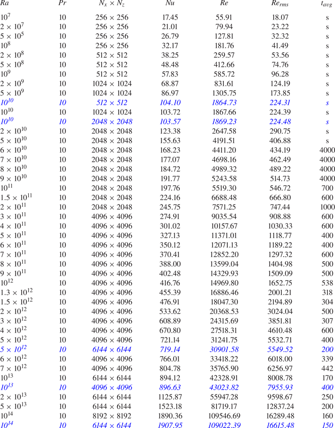


 Open access