


1. Introduction
Machine learning has developed many powerful techniques for solving prediction problems over the past few decades. Among these are prediction aggregation methods that seek to combine multiple machine learning models to make better predictions than can be achieved by individual predictors. This has strong theoretical foundations from the theory of meta-induction (Cesa-Bianchi and Lugosi Reference Cesa-Bianchi and Lugosi2006; Schurz Reference Schurz2019) as well as empirical support for the various methods (Dietterich Reference Dietterich, Kittler and Roli2000; Rokach Reference Rokach2010; Masoudnia and Ebrahimpour Reference Masoudnia and Ebrahimpour2014). Two important strategies for prediction aggregation are Bayesian model averages (BMAs) and mixtures of experts (MOEs). The former is a Bayesian method to make predictions by averaging predictions across a posterior of possible models learned from the data; the latter involves learning specialized machine learning models called experts and then making predictions based on which experts would make the best prediction based on observed features. BMA has been a widely preferred strategy because of strong theoretical guarantees about its inductive superiority. But surprisingly, MOE often performs better in practice, which has led to its adoption as a crucial element in many cutting-edge machine learning models like large language models. We aim to address this startling fact in this paper.
We argue that MOEs outperform BMAs because MOEs create more expressive hypotheses or models than BMAs. It can be shown that in at least one exact sense of capacity, an MOE can have greater capacity than a BMA composed of models similar to that MOE. We then validate this theoretical result with experiments that show that as the capacity required to predict a dataset grows, MOEs maintain good performance while BMAs fall off based on the capacity of their members. Both of these results suggest that the superiority of MOEs over BMAs, despite the latter’s inductive guarantees, stems from the restriction of BMAs to a poorer hypothesis class than MOEs.
The philosophical upshot of this finding is that MOEs can be thought of as doing abduction, in the Peircean sense of hypothesis construction, along with induction. In comparison, BMAs and other similar schemes are fundamentally inductive alone. We argue that MOEs demonstrate a divide-and-conquer strategy for hypothesis formation, similar to a suggestion given by Peirce. This means that MOE addresses a problem that Bayesian methods fail to address, which is where the hypothesis space comes from.
Importantly, this should be of interest to philosophers for two reasons. First, it provides a novel formal model for doing abduction in the Peircean sense. Second, it ties abduction to the rich mathematical framework of statistical learning theory, which could enable further formal theories to be produced.
Here is how our argument proceeds. First, we discuss MOEs as applied to supervised learning, i.e., learning from labeled data. Second, we review BMAs, reasons for their optimality, and empirical evidence pushing against that optimality. We discuss possible explanations for this difference but find them to be wanting. Third, we propose another explanation centered on the capacity of MOEs compared to BMAs. We show that with capacity made exact, we can prove that the capacity of MOEs will exceed the capacity of BMAs. Fourth, we build on this theoretical result by demonstrating experiments that show MOE performance maintains itself on datasets that require a certain amount of capacity to learn well while BMAs drop off. Fifth, we discuss the philosophical implications of this explanation, by highlighting that MOEs are essentially a form of abduction in the sense of hypothesis construction.
2. Mixtures of experts
In supervised learning, the goal of the machine learning algorithm is to predict some target $y$
from some vector of features
$y$
from some vector of features ${\bf{x}}$
(variables the model observes), and this goal is realized by training the model on some dataset of
${\bf{x}}$
(variables the model observes), and this goal is realized by training the model on some dataset of $n$
target and feature pairs
$n$
target and feature pairs ${\cal D} = {\{ \left( {{{\bf{x}}^{\left( i \right)}},{y^{\left( i \right)}}} \right)\} _{i = 1, \ldots, n}}$
, where
${\cal D} = {\{ \left( {{{\bf{x}}^{\left( i \right)}},{y^{\left( i \right)}}} \right)\} _{i = 1, \ldots, n}}$
, where ${\cal X}$
and
${\cal X}$
and ${\cal Y}$
are the training features and targets respectively. A model can be thought of as learning a probability function
${\cal Y}$
are the training features and targets respectively. A model can be thought of as learning a probability function $f(y|{\bf{x}},\theta )$
, where
$f(y|{\bf{x}},\theta )$
, where $\theta $
are the model parameters, from which predictions can be sampled or deterministically picked as the target with the highest probability, i.e., the prediction
$\theta $
are the model parameters, from which predictions can be sampled or deterministically picked as the target with the highest probability, i.e., the prediction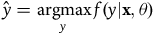 $\hat y = \mathop {{\rm{argmax}}}\limits_y f(y|{\bf{x}},\theta )$
. Training is accomplished by minimizing some loss or cost function
$\hat y = \mathop {{\rm{argmax}}}\limits_y f(y|{\bf{x}},\theta )$
. Training is accomplished by minimizing some loss or cost function $L\left( \theta \right)$
, which measures the dis-utility of a prediction error, through a training algorithm to find the best set of model parameters
$L\left( \theta \right)$
, which measures the dis-utility of a prediction error, through a training algorithm to find the best set of model parameters $\theta $
for making predictions. Models are then evaluated by how well they do on some hold-out test data set
$\theta $
for making predictions. Models are then evaluated by how well they do on some hold-out test data set ${\cal T} = {\{ \left( {{{\bf{x}}^{\left( i \right)}},{y^{\left( i \right)}}} \right)\} _{i = 1, \ldots, m}}$
not seen during training. The best models have the lowest loss on this test set.
${\cal T} = {\{ \left( {{{\bf{x}}^{\left( i \right)}},{y^{\left( i \right)}}} \right)\} _{i = 1, \ldots, m}}$
not seen during training. The best models have the lowest loss on this test set.
For example, suppose the problem is to predict blood pressure from body mass index (BMI). We treat our target $y$
as the continuous random variable blood pressure and our feature vector
$y$
as the continuous random variable blood pressure and our feature vector ${\bf{x}} = {[1,{x_1}]^{\rm{T }}}$
as the continuous random variable BMI,
${\bf{x}} = {[1,{x_1}]^{\rm{T }}}$
as the continuous random variable BMI, ${x_1}$
, and identity feature,
${x_1}$
, and identity feature, $1$
. A linear regression is then a normally distributed probability function
$1$
. A linear regression is then a normally distributed probability function ${f_{{\rm{lr}}}}(y|{\bf{x}},\theta )$
with known variance
${f_{{\rm{lr}}}}(y|{\bf{x}},\theta )$
with known variance ${\sigma ^2}$
and parameter vector
${\sigma ^2}$
and parameter vector $\theta = {[{\theta _0},{\theta _1}]^{\rm{T }}}$
, where
$\theta = {[{\theta _0},{\theta _1}]^{\rm{T }}}$
, where ${\theta _1}$
is the slope and
${\theta _1}$
is the slope and ${\theta _0}$
is the intercept, that characterize the mean of our distribution:
${\theta _0}$
is the intercept, that characterize the mean of our distribution:
 $${f_{{\rm{lr}}}}(y|{\bf{x}},\theta ) = {\cal N}\left( {{{\bf{x}}^{\rm{T }}}\theta, {\sigma ^2}} \right),$$
where ${{\bf{x}}^{\rm{T }}}$
is the transpose of our feature vector. Assuming statistical independence of our model parameters, we then fit our model by maximizing the likelihood
${{\bf{x}}^{\rm{T }}}$
is the transpose of our feature vector. Assuming statistical independence of our model parameters, we then fit our model by maximizing the likelihood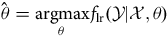 $\hat \theta = \mathop {{\rm{argmax}}}\limits_\theta {f_{{\rm{lr}}}}({\cal Y}|{\cal X},\theta )$
, which corresponds to minimizing the negative log-likelihood loss function
$\hat \theta = \mathop {{\rm{argmax}}}\limits_\theta {f_{{\rm{lr}}}}({\cal Y}|{\cal X},\theta )$
, which corresponds to minimizing the negative log-likelihood loss function ${L_{{\rm{NLL}}}}$
:
${L_{{\rm{NLL}}}}$
:
 $${L_{{\rm{NLL}}}}\left( \theta \right) = - \mathop {\mathop \sum \limits_{i = 1} }\limits^n {\rm{log}}\,\,{f_{{\rm{lr}}}}({y^{\left( i \right)}}|{{\bf{x}}^{\left( i \right)}},\theta ).$$
Due to our model being normally distributed and ignoring constants that do not depend on $\theta $
, the negative log-likelihood equates to minimizing the squared error:
$\theta $
, the negative log-likelihood equates to minimizing the squared error:
 $${L_{{\rm{NLL}}}}\left( \theta \right) = {1 \over {2{\sigma ^2}}}\mathop {\mathop \sum \limits_{i = 1} }\limits^n {({y^{\left( i \right)}} - {{\bf{x}}^{\left( i \right){\rm{T }}}}\theta )^2}.$$
We could then train our linear regression on the dataset ${\cal D}$
via gradient descent—an iterative optimization algorithm—to find the parameters that minimize this loss function. To evaluate how well our regression does, we evaluate its negative log-likelihood on a hold-out set of blood pressure and BMI pairs not seen during training. This is done because we want our model to inductively generalize from its training; we don’t want the model to have merely memorized the blood pressure and BMI pairs found in training. The best model is one that successfully minimizes the training loss while having the lowest test set loss.
${\cal D}$
via gradient descent—an iterative optimization algorithm—to find the parameters that minimize this loss function. To evaluate how well our regression does, we evaluate its negative log-likelihood on a hold-out set of blood pressure and BMI pairs not seen during training. This is done because we want our model to inductively generalize from its training; we don’t want the model to have merely memorized the blood pressure and BMI pairs found in training. The best model is one that successfully minimizes the training loss while having the lowest test set loss.
Aggregating predictions from many machine learning models is a common technique for improving predictive performance in supervised learning. There are two primary families of aggregation: ensemble methods and MOE methods.
In ensemble methods, we train individual models independently across the set of all training features ${\cal X}$
and then use some aggregation scheme across all models to produce a prediction. Examples of aggregation schemes include averaging and voting. In the averaging case, the prediction of an ensemble machine learning model
${\cal X}$
and then use some aggregation scheme across all models to produce a prediction. Examples of aggregation schemes include averaging and voting. In the averaging case, the prediction of an ensemble machine learning model $g\left( {\bf{x}} \right)$
is an average of
$g\left( {\bf{x}} \right)$
is an average of $n$
models with probabilities
$n$
models with probabilities $f(y|{\bf{x}},{\theta _i})$
parameterized by
$f(y|{\bf{x}},{\theta _i})$
parameterized by ${\theta _i}$
and weighted by weights
${\theta _i}$
and weighted by weights ${w_i}$
for
${w_i}$
for $i = 1, \ldots, n$
:
$i = 1, \ldots, n$
:
 $$g\left( {\bf{x}} \right) = \mathop {\mathop \sum \limits^n }\limits_{i = 1} {w_i}f(y|{\bf{x}},{\theta _i}).$$
The core intuition behind ensemble techniques is that they leverage the wisdom of the crowds: Instead of relying upon one highly specialized model for prediction, many models are consulted and then factored into the prediction. Betting markets in sports gambling can be thought of as an ensemble technique leveraging human gamblers as individual predictors, where the going price in the market corresponds to an average of all wagers. Examples of ensemble techniques include bagging, where the random predictors are trained and weighted on random subsets of data, and boosting, a technique where weak predictors are combined into stronger predictors by iteratively training predictors on their peers’ errors.
With an MOE (Jacobs et al. Reference Jacobs, Jordan, Nowlan and Hinton1991; Jordan and Jacobs Reference Jordan and Jacobs1994; Yuksel et al. Reference Yuksel, Wilson and Gader2012; Masoudnia and Ebrahimpour Reference Masoudnia and Ebrahimpour2014), models called experts specialize on elements of a partition of the feature set ${\cal X}$
, and predictions on a new sample from the mixture consist of routing the sample to the relevant experts based on where in that partition the sample falls. In the most general case where we route the sample to all experts, we employ weights for the experts that are a function of the sample features
${\cal X}$
, and predictions on a new sample from the mixture consist of routing the sample to the relevant experts based on where in that partition the sample falls. In the most general case where we route the sample to all experts, we employ weights for the experts that are a function of the sample features ${\bf{x}}$
. The MOE model
${\bf{x}}$
. The MOE model $h\left( {{\bf{x}};n} \right)$
with
$h\left( {{\bf{x}};n} \right)$
with $n$
experts then is a sum over experts with probability functions
$n$
experts then is a sum over experts with probability functions ${f_i}(y|{\bf{x}},{\theta _i})$
parameterized by
${f_i}(y|{\bf{x}},{\theta _i})$
parameterized by ${\theta _i}$
and a gating function
${\theta _i}$
and a gating function ${G_i}:{\cal X} \to \left[ {0,1} \right]$
for
${G_i}:{\cal X} \to \left[ {0,1} \right]$
for $i = 1, \ldots, n$
:
$i = 1, \ldots, n$
:
 $$h\left( {{\bf{x}};n} \right) = \mathop {\mathop \sum \limits^n }\limits_{i = 1} {G_i}\left( {\bf{x}} \right){f_i}(y|{\bf{x}},{\theta _i}).$$
The gating functions ${G_i}\left( {\bf{x}} \right)$
—a rule for assigning weights to the experts—are typically probabilities, such as the softmax (a function for converting numbers to probabilities) over a linear model. We say that experts are homogeneous when expert probability functions
${G_i}\left( {\bf{x}} \right)$
—a rule for assigning weights to the experts—are typically probabilities, such as the softmax (a function for converting numbers to probabilities) over a linear model. We say that experts are homogeneous when expert probability functions ${f_i}$
have the same form but are characterized by different parameters
${f_i}$
have the same form but are characterized by different parameters ${\theta _i}$
and inhomogeneous otherwise. For example, an MOE with only linear regressions as experts has homogeneous experts. Importantly, the gating function sometimes considers more than one expert in making a prediction—it sometimes assigns positive probability to multiple experts for a given sample. In those cases, the gating function is said to “softly partition” the feature set between experts, which means that it uses an expert’s predictions for more than one partition cell. The limiting case where only one expert is selected from a group of experts—where only one expert
${\theta _i}$
and inhomogeneous otherwise. For example, an MOE with only linear regressions as experts has homogeneous experts. Importantly, the gating function sometimes considers more than one expert in making a prediction—it sometimes assigns positive probability to multiple experts for a given sample. In those cases, the gating function is said to “softly partition” the feature set between experts, which means that it uses an expert’s predictions for more than one partition cell. The limiting case where only one expert is selected from a group of experts—where only one expert ${e_i}$
receives
${e_i}$
receives ${G_i}\left( {\bf{x}} \right) = 1$
and all the rest zero—makes this partition hard: each expert specializes on one and only one cell of a partition over
${G_i}\left( {\bf{x}} \right) = 1$
and all the rest zero—makes this partition hard: each expert specializes on one and only one cell of a partition over ${\cal X}$
. We will call this the top-expert MOE. In that case,
${\cal X}$
. We will call this the top-expert MOE. In that case, $h\left( {{\bf{x}};n} \right)$
is simply a piecewise function that applies the experts
$h\left( {{\bf{x}};n} \right)$
is simply a piecewise function that applies the experts ${e_i}\left( {\bf{x}} \right)$
Footnote 1 on
${e_i}\left( {\bf{x}} \right)$
Footnote 1 on ${\bf{x}}$
depending on what member of the partition
${\bf{x}}$
depending on what member of the partition ${Z_i} \in \left\{ {{Z_1}, \ldots, {Z_n}} \right\}$
of
${Z_i} \in \left\{ {{Z_1}, \ldots, {Z_n}} \right\}$
of ${\cal X}$
that
${\cal X}$
that ${\bf{x}}$
happens to belong in:
${\bf{x}}$
happens to belong in:
 $$h\left( {{\bf{x}};n} \right) = \left\{ {\matrix{ {{e_1}\left( {\bf{x}} \right),} \hfill & {{\bf{x}} \in {Z_1},} \hfill \cr {{e_2}\left( {\bf{x}} \right),} \hfill & {{\bf{x}} \in {Z_2},} \hfill \cr {{\rm{\;\;\;\;}} \vdots } \hfill & {{\rm{\;\;\;\;}} \vdots } \hfill \cr {{e_n}\left( {\bf{x}} \right),} \hfill & {{\bf{x}} \in {Z_n}.} \hfill \cr } } \right.$$
Here, expert ${e_1}$
only provides advice on cell
${e_1}$
only provides advice on cell ${Z_1}$
,
${Z_1}$
, ${e_2}$
on cell
${e_2}$
on cell ${Z_2}$
, and so on. The intuition behind MOE is familiar to consumers of medicine; when presented with symptoms, we will often go to the doctor we think is best specialized in diagnosing and treating illnesses that typically present those symptoms. If we happen to choose only one doctor for clinical advice, we employ the top-expert MOE, and if the doctors are all broadly similar in how they approach problems—say by receiving standard medical training instead of alternative medicine—then they are homogeneous.Footnote 2
${Z_2}$
, and so on. The intuition behind MOE is familiar to consumers of medicine; when presented with symptoms, we will often go to the doctor we think is best specialized in diagnosing and treating illnesses that typically present those symptoms. If we happen to choose only one doctor for clinical advice, we employ the top-expert MOE, and if the doctors are all broadly similar in how they approach problems—say by receiving standard medical training instead of alternative medicine—then they are homogeneous.Footnote 2
MOEs and ensembles, while both aggregation techniques, have important differences. Those differences consist of (i) how they are trained and (ii) how they aggregate predictions.
In the training regime, ensembles train their models separately and independently from their aggregation scheme. For example, in bagging (Breiman Reference Breiman1996), models are trained separately on random subsets of data drawn from ${\cal D}$
and only combined at inference time with their aggregation scheme. Boosting (Schapire Reference Schapire1990; Freund and Schapire Reference Freund, Schapire and Saitta1996) modifies this regime by training models sequentially on the whole data but weighting data samples by the errors of the previous model in the sequence to gradually scale up better predictors. In contrast, the experts and the gating function are all trained simultaneously in MOE; the gating function learns the relevant soft partition while the experts specialize in their particular region of data. This is done with either gradient descent or the expectation maximization algorithm. Unlike ensembles, this means the aggregation scheme is not done separately in inference but is crucial to the training process because of the tight connection between the gating function and the experts.
${\cal D}$
and only combined at inference time with their aggregation scheme. Boosting (Schapire Reference Schapire1990; Freund and Schapire Reference Freund, Schapire and Saitta1996) modifies this regime by training models sequentially on the whole data but weighting data samples by the errors of the previous model in the sequence to gradually scale up better predictors. In contrast, the experts and the gating function are all trained simultaneously in MOE; the gating function learns the relevant soft partition while the experts specialize in their particular region of data. This is done with either gradient descent or the expectation maximization algorithm. Unlike ensembles, this means the aggregation scheme is not done separately in inference but is crucial to the training process because of the tight connection between the gating function and the experts.
It is important to emphasize that the aggregation schemes between ensembles and MOEs differ in the relevance of the sample features for aggregating predictions. The critical difference lies in how we aggregate: In the ensemble method shown in equation 4, the weights ${w_i}$
are scalars and therefore are constant for all inputs, while in the MOE given in equation 5, the weights are determined by a gating function
${w_i}$
are scalars and therefore are constant for all inputs, while in the MOE given in equation 5, the weights are determined by a gating function ${G_i}\left( {\bf{x}} \right)$
, which explicitly makes the contribution of each expert conditional on the input sample’s features
${G_i}\left( {\bf{x}} \right)$
, which explicitly makes the contribution of each expert conditional on the input sample’s features ${\bf{x}}$
.Footnote 3 So aggregation proceeds very differently between ensembles and MOEs.
${\bf{x}}$
.Footnote 3 So aggregation proceeds very differently between ensembles and MOEs.
An extremely influential ensemble scheme is BMA, where all possible predictors of a certain class are considered by requiring the weights ${w_i}$
to be probabilities that reflect the posterior distribution of the model parameters given the data observed. This ensemble method has important theoretical guarantees, and we turn to discussing it now.
${w_i}$
to be probabilities that reflect the posterior distribution of the model parameters given the data observed. This ensemble method has important theoretical guarantees, and we turn to discussing it now.
3. Bayesian optimality
BMA receives its name from the application of Bayes’ rule to statistical and machine learning model prediction. Recall that Bayes’ rule states that if ${\theta _1},{\theta _2}, \ldots $
is a partition of model parameters, then the conditional probability of an element of that partition
${\theta _1},{\theta _2}, \ldots $
is a partition of model parameters, then the conditional probability of an element of that partition ${\theta _i}$
given some observed data
${\theta _i}$
given some observed data ${\cal D}$
is the ratio of the likelihood times the prior probability and the marginal probability of the data:Footnote 4
${\cal D}$
is the ratio of the likelihood times the prior probability and the marginal probability of the data:Footnote 4
 $$p({\theta _i}|{\cal D}) = {{p({\cal D}|{\theta _i})p\left( {{\theta _i}} \right)} \over {p\left( {\cal D} \right)}} = {{p({\cal D}|{\theta _i})p\left( {{\theta _i}} \right)} \over {\mathop {\mathop \sum \limits^\infty }\limits_{j = 1} p({\cal D}|{\theta _j})p\left( {{\theta _j}} \right)}}.$$
This is called the posterior probability, and it is applied in the posterior predictive distribution $p(y|{\bf{x}},{\cal D})$
, which is used to make a probabilistic prediction. The key idea is that predicting some target
$p(y|{\bf{x}},{\cal D})$
, which is used to make a probabilistic prediction. The key idea is that predicting some target $y$
from features
$y$
from features ${\bf{x}}$
and some previously observed data can be had by applying the law of total probability with respect to the model partition
${\bf{x}}$
and some previously observed data can be had by applying the law of total probability with respect to the model partition ${\theta _1},{\theta _2}, \ldots $
and weighting the model likelihoods by the posterior of the model given the data:
${\theta _1},{\theta _2}, \ldots $
and weighting the model likelihoods by the posterior of the model given the data:
 $$p(y|{\bf{x}},{\cal D}) = \mathop {\mathop \sum \limits^\infty }\limits_{i = 1} p(y|{\bf{x}},{\theta _i})p({\theta _i}|{\cal D}).$$
In essence, this states that if we average over all possible models by how likely it is that those models are correct given the data we have observed, then we can compute a posterior of the target given the observed data.Footnote 5 This has several desirable properties.
First, it allows us to form predictions with a natural regularizer. Regularization is a technique common in machine learning to combat overfitting. Overfitting is where a machine learning algorithm essentially does well on training data while failing to predict hold-out test data; the model “memorizes” the training data instead of truly learning the relevant “inductive patterns in the data.” An explanation for this behavior comes from the Probably, Approximately Correct (PAC) learning framework (Kearns and Vazirani Reference Kearns and Vazirani1994): models that overfit are too “complex” for the data.Footnote 6 Consequently, model complexity is penalized by an additional term in the loss function during training. This is called regularization, and the additional term in the loss function that penalizes complexity is called a regularizer. In the case of BMA, the posterior $p(\theta |{\cal D})$
builds in a natural regularizer with the prior
$p(\theta |{\cal D})$
builds in a natural regularizer with the prior $p\left( \theta \right)$
; if the model is a linear or polynomial regression and the prior is the standard normal, then the zero-centered prior assigns a lower probability to models with large parameter values, effectively penalizing model complexity similar to the complexity penalties in the Akaike and Bayesian information criteria. So BMA naturally provides better generalization and leads to “simpler” models over other aggregation techniques.
$p\left( \theta \right)$
; if the model is a linear or polynomial regression and the prior is the standard normal, then the zero-centered prior assigns a lower probability to models with large parameter values, effectively penalizing model complexity similar to the complexity penalties in the Akaike and Bayesian information criteria. So BMA naturally provides better generalization and leads to “simpler” models over other aggregation techniques.
Second, BMA produces models that have good decision-theoretic properties. We consider our loss function as capturing the relative dis-utility of making decisions, and a machine learning model as providing a decision rule (here we treat predictions as a type of action). Then, if we suppose there is a “true” parameter $\theta $
for generating the data
$\theta $
for generating the data ${\cal D}$
, we say the frequentist risk of a model is the likelihood of the data given the true-parameter-weighted expected value of that model’s loss. For example, when predicting the outcome of a sequence of coin tosses, the frequentist risk would be how well our model does on some loss for those tosses weighted by how likely each toss is given the bias of the coin. So supposing us to be realists about chances, the frequentist risk captures how well a machine learning model makes decisions relative to the true chances. This notion of risk has a tight connection to BMA. A BMA model is a Bayesian estimator in the sense that it minimizes the Bayes risk with respect to the posterior
${\cal D}$
, we say the frequentist risk of a model is the likelihood of the data given the true-parameter-weighted expected value of that model’s loss. For example, when predicting the outcome of a sequence of coin tosses, the frequentist risk would be how well our model does on some loss for those tosses weighted by how likely each toss is given the bias of the coin. So supposing us to be realists about chances, the frequentist risk captures how well a machine learning model makes decisions relative to the true chances. This notion of risk has a tight connection to BMA. A BMA model is a Bayesian estimator in the sense that it minimizes the Bayes risk with respect to the posterior $p(\theta |{\cal D})$
: the Bayes risk of a model with prior
$p(\theta |{\cal D})$
: the Bayes risk of a model with prior $\rho \left( \theta \right)$
is simply the
$\rho \left( \theta \right)$
is simply the $\rho \left( \theta \right)$
-weighted expected value of the frequentist risk. Instead of assuming a “true” parameter, we propose a prior probability distribution for the parameter and average out that prior across the frequentist risk. Suppose we are unsure what the true bias of a coin is when observing a sequence of coin tosses. Then we can consider the Bayes risk as putting a prior distribution over the bias and weighting the frequentist risk by that prior. If our model of the coin toss minimizes that risk, then we say it is a Bayesian estimator for the aforementioned prior. Consequently, it should be clear that a BMA model is a Bayes estimator concerning the posterior
$\rho \left( \theta \right)$
-weighted expected value of the frequentist risk. Instead of assuming a “true” parameter, we propose a prior probability distribution for the parameter and average out that prior across the frequentist risk. Suppose we are unsure what the true bias of a coin is when observing a sequence of coin tosses. Then we can consider the Bayes risk as putting a prior distribution over the bias and weighting the frequentist risk by that prior. If our model of the coin toss minimizes that risk, then we say it is a Bayesian estimator for the aforementioned prior. Consequently, it should be clear that a BMA model is a Bayes estimator concerning the posterior $p(\theta |{\cal D})$
because of how it is defined.
$p(\theta |{\cal D})$
because of how it is defined.
The so-called complete class theorems are an important property connecting the frequentist risk and the Bayes risk. These theorems state that Bayesian estimators form a complete class in the sense that any machine learning model that does better on the frequentist risk than any other model is a Bayesian estimator (Wald Reference Wald1947; Robert Reference Robert2007; Murphy Reference Murphy2022)Footnote 7 Critically, however, these optimality guarantees hold only within a fixed class of models. For example, a BMA composed of linear regression models can find the optimal linear predictor within the convex hull of the considered models, but it cannot generate a different type of model such as a quadratic predictor. Fixing the class appropriate class of models, the complete class theorems mean that there will be some Bayesian prior we can average over to equal the “correct” model of the data that does best on the loss; the hope is that we can then find that prior through our posterior by conditioning on the data. So, ideally, a BMA with enough data and non-perverse prior will be the Bayesian estimator that does as well as one can do on the frequentist risk. This should show up in terms of minimizing the loss on the hold-out test set.
With both of these desirable properties, it is then surprising that BMA is often outperformed by a MOE.
In figure 1, we show experiments involving a type of BMA and similar MOEs. The former is a Bayesian linear regression, which averages across a posterior ${\cal N}(\theta |\mu, {\rm{\Sigma }})$
all linear regressions given in equation 1, and the latter is an MOE involving two or more linear regressions as found in equation 1 (details can be found in the supplementary, appendix 2). Both models were trained on identical training data and evaluated on the same hold-out test data. The data consists of polynomials with some added normally distributed noise. Figure 1a shows the performance of these models on the mean squared error on hold-out test data, where lower is better; all mixture models match or exceed the performance of the Bayesian linear regression—with the greatest gap between the larger number of experts on higher-degree polynomials. Furthermore, since we control the data generation, we can directly calculate the frequentist risk. Again, the MOEs perform best here as seen in figure 1b, with the results closely tracking the mean squared error where lower is better. This collides with the expected hope that we should find the BMA model to do better here.
${\cal N}(\theta |\mu, {\rm{\Sigma }})$
all linear regressions given in equation 1, and the latter is an MOE involving two or more linear regressions as found in equation 1 (details can be found in the supplementary, appendix 2). Both models were trained on identical training data and evaluated on the same hold-out test data. The data consists of polynomials with some added normally distributed noise. Figure 1a shows the performance of these models on the mean squared error on hold-out test data, where lower is better; all mixture models match or exceed the performance of the Bayesian linear regression—with the greatest gap between the larger number of experts on higher-degree polynomials. Furthermore, since we control the data generation, we can directly calculate the frequentist risk. Again, the MOEs perform best here as seen in figure 1b, with the results closely tracking the mean squared error where lower is better. This collides with the expected hope that we should find the BMA model to do better here.
Plots of the mean squared error and frequentist risk for Bayesian linear regressions and MOE with $\left[ {2,3,4} \right]$
expert linear regressions on polynomial datasets of degrees
$\left[ {2,3,4} \right]$
expert linear regressions on polynomial datasets of degrees $\left[ {1,2,3,4,5} \right]$
. Lower mean squared error and frequentist risk is better.
$\left[ {1,2,3,4,5} \right]$
. Lower mean squared error and frequentist risk is better.

One might think that these results are due to the MOEs employing more sophisticated experts, such as polynomial regressions, or a non-probabilistic aggregation scheme, but that is not the case. Both the Bayesian linear regression and the MOEs average over linear regressions, i.e., the MOEs are homogenous: each expert is accounted for in the Bayesian linear regression, and those experts receive some weighted probability according to the posterior. If anything, the MOEs employ fewer experts since a BMA averages across all possible expert configurations while the most we consider in our experiments are four experts. Furthermore, the averaging scheme employed here is not all that different; both the Bayesian linear regression and the MOEs weight their subcomponent models by probabilities. In fact, the Bayesian linear regression does things the right way by weighting the models by a data-driven posterior. So the difference between the two cannot be due to better experts or a non-probabilistic approach to aggregation.
The ability of MOE to outperform ensembles like BMA has led them to be an important component of contemporary machine learning techniques. For example, Yuksel et al. (Reference Yuksel, Wilson and Gader2012) cite a 2008 survey of then-important machine learning methods and argue that MOE outperforms all of them (Yuksel et al. Reference Yuksel, Wilson and Gader2012, 1178). They cite in particular the advantages an MOE model has over the popular ensemble method of boosting (Yuksel et al. Reference Yuksel, Wilson and Gader2012, 1187–88). Furthermore, Masoudnia and Ebrahimpour (Reference Masoudnia and Ebrahimpour2014) argue that MOE consistently outperforms popular ensemble techniques like bagging and boosting (Masoudnia and Ebrahimpour Reference Masoudnia and Ebrahimpour2014, 286–87). This is despite the challenges MOE faces in learning the right partition and gating function (see Masoudnia and Ebrahimpour (Reference Masoudnia and Ebrahimpour2014, sec. 3.3)). Those challenges have increasingly been overcome through sparsity, i.e., only selecting the top- $k$
experts when making predictions, and noisy gating, i.e., injecting noise during the training process to force the gating function to use all experts (Shazeer et al. Reference Shazeer, Mirhoseini, Maziarz, Davis, Le, Hinton and Dean2017). This has led to MOEs being an increasingly important component of large language models, like OpenAI’s GPT-4 (Betts Reference Betts2024) and Mistral’s Mixtral (Jiang et al. Reference Jiang, Sablayrolles, Roux, Mensch, Savary, Bamford, Singh Chaplot, Casas, Hanna, Bressand, Lengyel, Bour, Lample, Lavaud, Saulnier, Lachaux, Stock, Subramanian, Yang, Antoniak, Scao, Gervet, Lavril, Wang, Lacroix and Sayed2024).
$k$
experts when making predictions, and noisy gating, i.e., injecting noise during the training process to force the gating function to use all experts (Shazeer et al. Reference Shazeer, Mirhoseini, Maziarz, Davis, Le, Hinton and Dean2017). This has led to MOEs being an increasingly important component of large language models, like OpenAI’s GPT-4 (Betts Reference Betts2024) and Mistral’s Mixtral (Jiang et al. Reference Jiang, Sablayrolles, Roux, Mensch, Savary, Bamford, Singh Chaplot, Casas, Hanna, Bressand, Lengyel, Bour, Lample, Lavaud, Saulnier, Lachaux, Stock, Subramanian, Yang, Antoniak, Scao, Gervet, Lavril, Wang, Lacroix and Sayed2024).
Two explanations have been given for the superiority of MOE over ensemble methods like BMA. First, MOEs work well on data generated by oxymoronic one-to-many functions, i.e., “functions” that can map a single input to multiple outputs, whereas traditional models and ensembles cannot learn this data (Murphy Reference Murphy2022, 454). However, this explanation fails in the experiments described above: all of the datasets were generated by proper functions that pass the vertical line test. Second, MOEs supposedly work well due to experts learning data that is negatively correlated (Masoudnia and Ebrahimpour Reference Masoudnia and Ebrahimpour2014, 287). While this is true for some data, it is not always the case, as can be seen in the aforementioned experiments on degree-three polynomials where different elements of the data are either positively correlated or not correlated at all. So both of these explanations seem unnecessary for explaining why MOE does well.
Recapping, an important class of ensemble models are Bayesian ones. These models have attractive theoretical features such as regularization and accuracy considerations. But these models are often outperformed by MOEs, as demonstrated by some experiments. This has led to a general adoption of MOEs in machine learning for hard problems over ensemble schemes, such as in large language models. Two reasons for this superiority are that MOEs can fit data generated by one-to-many “functions” and that MOEs train their experts on negatively correlated data. But better performance can be found on proper functions and the partition learned need not involve negative correlations. So another explanation should be given, which we turn to now.
4. The functional capacity of models
A plausible, intuitive hypothesis for why MOEs outperform ensemble techniques like BMA is that MOEs have greater functional capacity than ensembles. That is, MOEs characterize hypothesis classes that have a richer set of labeling schemes than ensembles like BMA, and so the improved performance relative to provably “better” methods like BMA is due to BMA being restricted to a more impoverished model class. This shows up in the experiments in section 3, where we see that the various MOEs continue to do well on mean squared error loss as the degree of the polynomial data scales. The Bayesian is in some sense limited by only considering linear regressions, while the MOEs seem able to stitch together multiple functions—despite the MOEs, like the BMA, only using linear regressions.
To make this hypothesis exact, we need to do two things. First, we need to specify what is a good explication of functional capacity, and second, we need to show how, in principle, at least some MOEs have a greater functional capacity than a BMA.
The intuitive idea of the functional capacity of a model is supposed to be something like the set of functions the model can learn. What counts as a relevant function depends on the problem the machine learning model solves. In supervised learning, those problems are sorted into the buckets of regression and classification, which correspond to predicting continuous targets or discrete targets respectively. With classification, the prediction problem is one of separating data into sets identified with the target, and the complexity of the problem is in some sense dependent on the data being used—predicting the label of a picture from raw pixels is harder than predicting from a higher-level feature like the presence or absence of an animal. Measuring how well we can separate data is the core intuition behind the Vapnik–Chervonenkis dimension (VC dimension). A more sophisticated model with higher functional capacity will be one that can better sort more complex data into classes; VC dimension gives us an exact measure of that capacity in terms of the cardinality of the data. This makes it a good explication of functional capacity because it specifies the type of functions a model can fit by one important sense of the complexity of the data in the classification problem at hand.
To define VC dimension, we need to define what it means to separate data, i.e., to shatter a dataset. Our context is binary classification, where machine learning models are treated as functions that map between features ${\cal X}$
and the binary labels
${\cal X}$
and the binary labels $\left\{ {0,1} \right\}$
. For example, we might be interested in classifying whether a picture is of a cat or not. We then group our binary classifiers into sets
$\left\{ {0,1} \right\}$
. For example, we might be interested in classifying whether a picture is of a cat or not. We then group our binary classifiers into sets ${\cal H}$
and specify that
${\cal H}$
and specify that ${\cal H}$
shatters some dataset
${\cal H}$
shatters some dataset $X$
if for any arbitrary labeling of
$X$
if for any arbitrary labeling of $X$
there is a classifier in
$X$
there is a classifier in ${\cal H}$
that correctly classifies that labeling.
${\cal H}$
that correctly classifies that labeling.
Definition 4.1.
Let ${\cal H}$
be a set of binary classifiers
${\cal H}$
be a set of binary classifiers $h:{\cal X} \to \left\{ {0,1} \right\}$
. Given a set of points
$h:{\cal X} \to \left\{ {0,1} \right\}$
. Given a set of points $X = \left\{ {{x^{\left( 1 \right)}}, \ldots, {x^{\left( m \right)}}} \right\}$
where
$X = \left\{ {{x^{\left( 1 \right)}}, \ldots, {x^{\left( m \right)}}} \right\}$
where ${x^{\left( i \right)}} \in {\cal X}$
, we say that
${x^{\left( i \right)}} \in {\cal X}$
, we say that ${\cal H}$
shatters
${\cal H}$
shatters $X$
if for any labels
$X$
if for any labels $Y = \left\{ {{y^{\left( 1 \right)}}, \ldots, {y^{\left( m \right)}}} \right\}$
where
$Y = \left\{ {{y^{\left( 1 \right)}}, \ldots, {y^{\left( m \right)}}} \right\}$
where ${y^{\left( i \right)}} \in \left\{ {1,0} \right\}$
, there exists
${y^{\left( i \right)}} \in \left\{ {1,0} \right\}$
, there exists $h \in {\cal H}$
such that
$h \in {\cal H}$
such that $h\left( {{x^{\left( i \right)}}} \right) = {y^{\left( i \right)}}$
for
$h\left( {{x^{\left( i \right)}}} \right) = {y^{\left( i \right)}}$
for $i = 1, \ldots, m$
.
$i = 1, \ldots, m$
.
Suppose our set of models are all linear classifiers, i.e., they classify by drawing lines to separate data. Then, as can be seen in figure 2, this class can shatter a given set of three points in ${\mathbb{R}^2}$
as seen in figure 2a, but there is no set of four points that it can shatter as seen in figure 2b. It shatters the former because regardless of how we label those three points, some line can separate them, which implies there is some linear classifier that can make a completely correct and error-free identification of the targets. It fails to shatter the latter because those four points have a labeling that no line can cleanly separate error-free.
${\mathbb{R}^2}$
as seen in figure 2a, but there is no set of four points that it can shatter as seen in figure 2b. It shatters the former because regardless of how we label those three points, some line can separate them, which implies there is some linear classifier that can make a completely correct and error-free identification of the targets. It fails to shatter the latter because those four points have a labeling that no line can cleanly separate error-free.
An example of shattering and failing to shatter. Figure 2a shows a set of points that can be shattered by the set of linear classifiers because any arbitrary labeling, i.e., which points are assigned blue or red, can be correctly classified by at least some linear classifier, i.e., we can draw a line separating the two labels without any mistakes. Figure 2b shows a set of points that cannot be shattered by that set since no line can separate this particular coloring without any errors.

The VC dimension of a class ${\cal H}$
is then the cardinal size of the largest set of data, with respect to some space of possible data like
${\cal H}$
is then the cardinal size of the largest set of data, with respect to some space of possible data like $\mathbb{R}$
, that that class can shatter.
$\mathbb{R}$
, that that class can shatter.
Definition 4.2 The Vapnik–Chervonenkis dimension of a set of binary classifiers $VCD\left( {\cal H} \right)$
defined over instance space
$VCD\left( {\cal H} \right)$
defined over instance space ${\cal X}$
is the cardinality of the largest finite subset of
${\cal X}$
is the cardinality of the largest finite subset of ${\cal X}$
that
${\cal X}$
that ${\cal H}$
can shatter. If arbitrarily large subsets can be shattered, then
${\cal H}$
can shatter. If arbitrarily large subsets can be shattered, then $VCD\left( {\cal H} \right): = \infty $
.
$VCD\left( {\cal H} \right): = \infty $
.
For example, linear classifiers in the Cartesian plane can shatter any three-point labeling, but for any four points there will be a labeling that cannot be shattered. So the VC dimension of the set of linear classifiers concerning ${\mathbb{R}^2}$
will be exactly three.
${\mathbb{R}^2}$
will be exactly three.
It should be noted that VC dimension is not correlated with parameter count: one can have a high VC dimension with a low parameter count. For example, the set of models given by $I\left( {{\rm{sin}}\alpha \cdot {\bf{x}}} \right)$
, where
$I\left( {{\rm{sin}}\alpha \cdot {\bf{x}}} \right)$
, where $I\left( x \right)$
is the indicator function that assumes
$I\left( x \right)$
is the indicator function that assumes $1$
if
$1$
if $x \gt 0$
and
$x \gt 0$
and $0$
otherwise, has only one parameter
$0$
otherwise, has only one parameter $\alpha \in \mathbb{R}$
but an infinite VC dimension (Hastie et al. Reference Hastie, Tibshirani and Friedman2009, 237). This makes VC dimension a better characterization of model functional capacity than raw parameter count since the above model intuitively is more complex than a linear classifier—even though the linear classifier has more parameters.
$\alpha \in \mathbb{R}$
but an infinite VC dimension (Hastie et al. Reference Hastie, Tibshirani and Friedman2009, 237). This makes VC dimension a better characterization of model functional capacity than raw parameter count since the above model intuitively is more complex than a linear classifier—even though the linear classifier has more parameters.
Importantly, ensembles have a maximum VC dimension given by the number of ensemble members and the base VC dimension of the class of members used in the set of ensemble hypotheses. Let $L\left( {{\cal H},n} \right)$
be the set of binary classifiers that are linear combinations of hypotheses drawn from binary classifiers
$L\left( {{\cal H},n} \right)$
be the set of binary classifiers that are linear combinations of hypotheses drawn from binary classifiers ${\cal H}$
, i.e.,
${\cal H}$
, i.e., $L\left( {{\cal H},n} \right) = \left\{ {x \mapsto sgn\left( {\mathop \sum \nolimits_{i = 1}^n {w_i}{f_i}\left( x \right)} \right):{\bf{w}} \in {{\mathbb R}^n},\forall i,{f_i} \in {\cal H}} \right\}$
, where
$L\left( {{\cal H},n} \right) = \left\{ {x \mapsto sgn\left( {\mathop \sum \nolimits_{i = 1}^n {w_i}{f_i}\left( x \right)} \right):{\bf{w}} \in {{\mathbb R}^n},\forall i,{f_i} \in {\cal H}} \right\}$
, where $sgn$
is the signum function, which returns
$sgn$
is the signum function, which returns $ + 1$
for positive or zero inputs and
$ + 1$
for positive or zero inputs and $ - 1$
for negative inputs. By definition, every ensemble will be in this set. Then it can be shown that if
$ - 1$
for negative inputs. By definition, every ensemble will be in this set. Then it can be shown that if $VCD\left( {\cal H} \right) = m$
is finite for some finite
$VCD\left( {\cal H} \right) = m$
is finite for some finite $m \gt 3$
, then
$m \gt 3$
, then $VCD\left( {L\left( {{\cal H},n} \right)} \right) \le \tilde O\left( {mn} \right)$
, where
$VCD\left( {L\left( {{\cal H},n} \right)} \right) \le \tilde O\left( {mn} \right)$
, where $\tilde O$
means we ignore any constants or logarithmic terms (Shalev-Shwartz and Ben-David Reference Shalev-Shwartz and Ben-David2014, 109).Footnote 8 This is effectively to say that the VC dimension of ensembles with
$\tilde O$
means we ignore any constants or logarithmic terms (Shalev-Shwartz and Ben-David Reference Shalev-Shwartz and Ben-David2014, 109).Footnote 8 This is effectively to say that the VC dimension of ensembles with $n$
members and whose members have a VC dimension
$n$
members and whose members have a VC dimension $m$
is no bigger than
$m$
is no bigger than $nm$
. While these bounds do not technically apply to BMAs, since BMAs consider infinitely many hypotheses, in practice they do because almost all BMAs are approximated through finite sampling schemes, i.e., Monte Carlo methods. Crucially, this is an upper bound: It can be shown in many cases that the VC dimension is significantly less—sometimes it is exactly the same VC dimension as the base class
$nm$
. While these bounds do not technically apply to BMAs, since BMAs consider infinitely many hypotheses, in practice they do because almost all BMAs are approximated through finite sampling schemes, i.e., Monte Carlo methods. Crucially, this is an upper bound: It can be shown in many cases that the VC dimension is significantly less—sometimes it is exactly the same VC dimension as the base class ${\cal H}$
(see Shalev-Shwartz and Ben-David (Reference Shalev-Shwartz and Ben-David2014, 113), exercise 10.4, for examples). The upshot is that ensembles are bounded above by the number of members and the capacity of those members to separate data.
${\cal H}$
(see Shalev-Shwartz and Ben-David (Reference Shalev-Shwartz and Ben-David2014, 113), exercise 10.4, for examples). The upshot is that ensembles are bounded above by the number of members and the capacity of those members to separate data.
MOE, however, can be shown to have a higher VC dimension than the experts it employs. Jiang (Reference Jiang2000) showed that for mixtures of $n$
Bernoulli binary classifiers on
$n$
Bernoulli binary classifiers on $\mathbb{R}$
, the VC dimension is exactly
$\mathbb{R}$
, the VC dimension is exactly $n$
, and for logistic regressions or Bernoulli binary classifiers on the instance space of
$n$
, and for logistic regressions or Bernoulli binary classifiers on the instance space of ${\mathbb{R}^d}$
, the VC dimension can be bounded below by the number of experts
${\mathbb{R}^d}$
, the VC dimension can be bounded below by the number of experts $n$
and from above to the worst case
$n$
and from above to the worst case $O\left( {{n^4}{d^2}} \right)$
(Jiang Reference Jiang2000, 7). These bounds can be tightened on
$O\left( {{n^4}{d^2}} \right)$
(Jiang Reference Jiang2000, 7). These bounds can be tightened on $\mathbb{R}$
. First, we say a set of functions
$\mathbb{R}$
. First, we say a set of functions ${\cal F}$
whose domain is the reals is closed under translation just in case, for any function
${\cal F}$
whose domain is the reals is closed under translation just in case, for any function $f$
in that set and any
$f$
in that set and any $a \in \mathbb{R}$
, the function
$a \in \mathbb{R}$
, the function ${f_a}\left( {x + a} \right)$
is also in
${f_a}\left( {x + a} \right)$
is also in ${\cal F}$
. Examples of these sets will be the set of all linear binary classifiers, the set of all polynomial binary classifiers of some positive degree
${\cal F}$
. Examples of these sets will be the set of all linear binary classifiers, the set of all polynomial binary classifiers of some positive degree $d$
, and the set of all feedforward neural networks (a prominent type of artificial neural network where information flows in only one direction) whose domains are the reals.Footnote 9 Second, suppose we restrict ourselves to a limiting case involving top-expert MOEs with homogeneous experts drawn from a class closed under translation. In that case, we can show that the VC dimension will have a lower bound that is a product of the number of experts and those experts’ VC dimension.Footnote 10
$d$
, and the set of all feedforward neural networks (a prominent type of artificial neural network where information flows in only one direction) whose domains are the reals.Footnote 9 Second, suppose we restrict ourselves to a limiting case involving top-expert MOEs with homogeneous experts drawn from a class closed under translation. In that case, we can show that the VC dimension will have a lower bound that is a product of the number of experts and those experts’ VC dimension.Footnote 10
Proposition 4.3 Let ${\cal H}$
be a set of top-expert mixture of experts binary classifiers of
${\cal H}$
be a set of top-expert mixture of experts binary classifiers of $n$
homogeneous binary classifier experts drawn from the set
$n$
homogeneous binary classifier experts drawn from the set ${\cal E}$
closed under translation with
${\cal E}$
closed under translation with $VCD\left( {\cal E} \right) = m$
defined over instance space
$VCD\left( {\cal E} \right) = m$
defined over instance space $\mathbb{R}$
. Then
$\mathbb{R}$
. Then $VCD\left( {\cal H} \right)nm$
for
$VCD\left( {\cal H} \right)nm$
for $\mathbb{R}$
.
$\mathbb{R}$
.
What this means is that at least some MOEs have a higher VC dimension than BMAs and so greater functional capacity. They can fit more complex data and so involve fundamentally more complex hypotheses. The intuition behind Proposition 4.3 can be seen by observing that a top-expert MOE with homogenous experts is a piecewise function that deploys each expert on exactly one element of a partition of the feature space; such a piecewise function will be able to separate more complex data than any of its components individually. Likewise, non-top-expert MOEs will form similar piecewise functions, though of possibly less complexity depending on the soft partition learned by the gating function. The upshot is that with functional capacity understood as VC dimension, we can vouchsafe the earlier intuition that MOEs have greater “capacity” and can learn more complex functions than ensembles like BMA.
This means that comparing MOEs to BMAs is an apples-to-oranges comparison. If MOE and Bayesian models are restricted to sub-models with the same complexity, then MOE will have an inherent advantage on more complex datasets like those observed in section 3. Provide the Bayesian the right type of models and that advantage will likely disappear.
In summary, we have argued that an intuitive explanation for the superiority of MOE over ensembles like BMA—despite the theoretical reasons for the Bayesian to be advantaged—is the greater functional capacity of MOEs. We argued that VC dimension is a good explication of that capacity, and we proved that the VC dimension of some MOEs will be greater than a BMA over models with the same capacity as the MOE. However, theoretical considerations can only cut so much ice. The question is whether MOEs, such as those that are not top-experts, can do well on datasets that exactly track greater VC dimensions. We turn to that now.
5. Experiments
The discussion and results in section 4 provide a theoretical reason why MOEs may have greater functional capacity than ensembles like BMAs, but does this show up empirically? Two problems prevent an immediate acceptance of this fact. First, Proposition 4.3 only applies to top-expert MOEs but most MOEs in practice have multiple experts per partition; second, the proposition applies only if the top-expert MOE is learned when this may often prove difficult or impossible in practice.Footnote 11 Consequently, we should empirically validate our theoretical results. We address this worry here by detailing experiments involving datasets that stand as a proxy for the VC dimension of binary classifiers.
Our method for building datasets with a correlated VC dimension takes advantage of the fact that polynomial binary classifiers of degree $m$
over instance space
$m$
over instance space ${\mathbb{R}^d}$
have a VC dimension of
${\mathbb{R}^d}$
have a VC dimension of $\left( {\matrix{ {d + m} \hfill \cr d } } \right)$
(Shalev-Shwartz and Ben-David Reference Shalev-Shwartz and Ben-David2014, 57). We can then use those binary classifiers to generate datasets that in fact will be classifiable by machine learning models with the appropriate VC dimension. An example dataset can be seen in figure 3. We build a polynomial binary classifier of degree
$\left( {\matrix{ {d + m} \hfill \cr d } } \right)$
(Shalev-Shwartz and Ben-David Reference Shalev-Shwartz and Ben-David2014, 57). We can then use those binary classifiers to generate datasets that in fact will be classifiable by machine learning models with the appropriate VC dimension. An example dataset can be seen in figure 3. We build a polynomial binary classifier of degree $m$
with coefficients
$m$
with coefficients $\left[ {{\theta _m}, \ldots, {\theta _0}} \right]$
, and then we generate points in
$\left[ {{\theta _m}, \ldots, {\theta _0}} \right]$
, and then we generate points in ${\mathbb{R}^2}$
around that polynomial with a normal distribution. Points that lie above the polynomial are assigned one label and those below another label. We say this dataset has a correlated VC dimension of
${\mathbb{R}^2}$
around that polynomial with a normal distribution. Points that lie above the polynomial are assigned one label and those below another label. We say this dataset has a correlated VC dimension of $\left( {\matrix{ {2 + m} \hfill \cr 2 } } \right)$
since we can achieve near-perfect accuracy by fitting a logistic regression with a design matrix that is a degree-
$\left( {\matrix{ {2 + m} \hfill \cr 2 } } \right)$
since we can achieve near-perfect accuracy by fitting a logistic regression with a design matrix that is a degree- $m$
polynomial.
$m$
polynomial.
Example of a VC dimension polynomial dataset, degree 3. Red indicates the polynomial binary classifier assigns label $0$
and blue indicates the classifier assigns label
$0$
and blue indicates the classifier assigns label $1$
. The resulting correlated VC dimension is
$1$
. The resulting correlated VC dimension is $\left( {\matrix{ 5 \hfill \cr 2 \hfill \cr } } \right) = 10$
.
$\left( {\matrix{ 5 \hfill \cr 2 \hfill \cr } } \right) = 10$
.

Our chosen binary classifiers for the experiments are logistic regressions. A logistic regression is a binary linear classifier with likelihood ${f_\sigma }(y|{\bf{x}},\theta )$
where
${f_\sigma }(y|{\bf{x}},\theta )$
where $\theta = {[{\theta _0}, \ldots, {\theta _d}]^{\rm{T }}}$
and
$\theta = {[{\theta _0}, \ldots, {\theta _d}]^{\rm{T }}}$
and ${\bf{x}} = {[1,{x_1}, \ldots, {x_d}]^{\rm{T }}}$
such that
${\bf{x}} = {[1,{x_1}, \ldots, {x_d}]^{\rm{T }}}$
such that
 $${f_\sigma }(y|{\bf{x}},\theta ) = {\rm{Ber}}(y|\sigma \left( {{{\bf{x}}^{\rm{T }}}\theta } \right)).$$
Here, Ber is the Bernoulli distribution and $\sigma $
is the logistic sigmoid function
$\sigma $
is the logistic sigmoid function $\sigma \left( x \right) = 1/\left[ {1 + {\rm{exp}}\left( { - x} \right)} \right]$
. Our MOEs consist of two to four experts that are logistic regressions that employ a top-two expert configuration, and we choose a BMA that averages over logistic regressions. Unfortunately, there are no analytically computable posteriors
$\sigma \left( x \right) = 1/\left[ {1 + {\rm{exp}}\left( { - x} \right)} \right]$
. Our MOEs consist of two to four experts that are logistic regressions that employ a top-two expert configuration, and we choose a BMA that averages over logistic regressions. Unfortunately, there are no analytically computable posteriors $p(\theta |{\cal D})$
for logistic regressions, so we have to approximate it for the BMA (see supplementary, appendix 2 for details).
$p(\theta |{\cal D})$
for logistic regressions, so we have to approximate it for the BMA (see supplementary, appendix 2 for details).
All models were trained to minimize the cross-entropy loss function (a type of loss function for categorical targets) using stochastic gradient descent (a variant of gradient descent that estimates the gradient via random samples) on a training set, and we then evaluated them on a hold-out test set. The results can be seen in figure 4.
The hold-out test set accuracy and loss of stochastic gradient Hamiltonian Monte Carlo (SGHMC) and variational inference (VI) logistic regression (LR) BMAs and logistic regression MOEs. For accuracy in figure 4a, higher is better; for loss in figure 4b, lower is better. We see that as the VC dimension increases, the accuracy and loss of the BMAs falls off, while the accuracy of the MOEs stays relatively constant, with some degradation in the two-expert model.

The experiments show that at a correlated VC dimension of $3$
, the Bayesian models perform roughly on par with the MOEs, but then there is considerable separation as the VC dimension of the dataset climbs. Figure 4a shows that BMAs consistently underperform on test-set accuracy, only doing modestly better than chance; however, the MOEs perform well as the VC dimension continues to climb, though the MOE with two experts shows degraded accuracy relative to the other models. In figure 4b, we see the same trends on test-set accuracy reflected in the cross-entropy loss: the Bayesian models approach the loss on hold-out test data as the MOEs, but then underperform as the VC dimension climbs. Again, the two-expert MOE model shows degradation more so than the higher expert counts.
$3$
, the Bayesian models perform roughly on par with the MOEs, but then there is considerable separation as the VC dimension of the dataset climbs. Figure 4a shows that BMAs consistently underperform on test-set accuracy, only doing modestly better than chance; however, the MOEs perform well as the VC dimension continues to climb, though the MOE with two experts shows degraded accuracy relative to the other models. In figure 4b, we see the same trends on test-set accuracy reflected in the cross-entropy loss: the Bayesian models approach the loss on hold-out test data as the MOEs, but then underperform as the VC dimension climbs. Again, the two-expert MOE model shows degradation more so than the higher expert counts.
These results validate empirically the theoretical results from section 4. Note that the bound proved in Proposition 4.3 is a lower bound for top-experts, so the VC dimension of the MOEs may be higher. The upshot is that we have both theoretical and empirical reasons to suggest that our explanation for the superiority MOEs over ensembles like BMA is correct: MOEs can simply learn more expressive hypotheses than averaging schemes like BMAs.
6. Mixtures of experts as abductive modeling
The argument from the previous sections has been that MOEs outperform averaging schemes like the Bayesian ones because they avail themselves of a richer hypothesis space. What is very interesting about this is that they find themselves in that bigger hypothesis space by way of simpler hypotheses; the experts, as noted, have a lower functional capacity than the MOE as a whole. Through the gating function, the feature space is soft-partitioned into cells that expert models can then specialize on. Importantly, this allows a virtuous learning process that enables experts to master relatively narrow domains while ensuring that collectively the experts build a more sophisticated, broader picture of the problem at hand. We argue in this section that this process is a form of abduction in the Peircean sense of hypothesis construction. This explains the fundamental difference between MOE and BMA: the former combines abduction and induction while the latter only uses induction.
A big assumption of the Bayesian approach to inductive reasoning is that the hypothesis space must be given. We have an algebra (or sigma-algebra) that captures in some sense all of the questions that we want to have answered in our inquiry and evidence we could bear on those questions. Then we proceed in our inquiry by considering some partition that is a subset of that algebra that characterizes the relevant scientific hypotheses and applying Bayes’ rule on new evidence as it comes in to update ourselves on our credences in the members of that partition. The assumption about the hypothesis space shows up twice here: first, in the granted algebra that characterizes inquiry, and second, in the selected hypothesis partition used when applying Bayes’ rule. We see both assumptions play a crucial role in BMA. The initial algebra is the possible model parameters and the range of values the feature and target random variables may assume, and the hypothesis partition is the range of possible model parameters assumed. With this fixed, no further hypothesis or evidence may be admitted into the averaging scheme. So BMA perfectly embodies the Bayesian approach—an approach that is fundamentally an inductive one.
By an inductive approach, we mean an ampliative inference from evidence to hypotheses. For the Bayesian, this can be thought of as a type of diachronic coherence between our current partial beliefs and our future partial beliefs; we change our beliefs in such a way as to avoid sure losses when gambling on those beliefs (Zabell Reference Zabell2005, 132–33). In that sense, BMA is induction par excellence—we aim to make predictions of new data based on what we have observed from old data in a probabilistic manner that guarantees we do as best we can by a loss function that captures the modeler’s subjective utility function on the prediction problem. The main assumption we make is that some class of models best parameterizes the predictive problem, and so we learn about those models based on the data we have observed in a diachronically coherent manner. Then, when we make our predictions, we factor what we have learned about those models into our predictions.
While MOE certainly does induction too, there is an additional element not present in the Bayesian approach. MOE partitions the input feature space and then through the gating function routes predictive samples to experts based on where they fall in that partition. This is termed a divide-and-conquer strategy or conditional computation since the MOE learns how best to divide a problem into sub-problems that can more easily be addressed by expert models. In contrast, BMAs learn no such partition, nor do they break down the problem into more easily addressable sub-problems. This divide-and-conquer approach is chiefly responsible for MOE’s expressive advantage over ensemble methods.
We argue that the MOE approach to the problem of prediction in machine learning is exactly an approach germane to abductive inference or hypothesis construction.
What we mean here by abductive inference or abduction is hypothesis construction or generation. The problem of hypothesis construction was articulated by C. S. Peirce as a form of conjecturing (Peirce Reference Peirce1901). He thinks that this is perhaps the most important element of scientific inquiry, and he discusses several principles to be applied when conjecturing hypotheses. Among those to consider is the economies of research—the resources spent finding hypotheses and testing them—which are important because we should expect our candidate hypotheses to break down and our time and resources in inquiry limited. He proposes several qualities to guide hypothesis selection (Peirce Reference Peirce1901, 109). One in the current context stands out. He calls this “Caution” and what he means is adopting a strategy of hypothesis formation that breaks down the problem space into regions that allow for groups of hypotheses to be quickly tested and discarded by their sub-components to converge at the best candidate in the most expeditious manner, and he proposes to illustrate the idea with a game. While there is some ambiguity about what Peirce means here, one plausible interpretation is that hypothesis construction should proceed with an eye toward the logical parts of the hypothesis and how they can be structured in a way to facilitate a divide-and-conquer search when testing the hypothesis. We select a hypothesis based on how fruitfully its components divide up the testing space. That selection strategy functions as an integral component in abductive reasoning.
The same divide-and-conquer strategy goes on in MOE at the time of inference where a complex sample is routed to a region where a smaller, simpler component can be used to make a prediction. An MOE model as a hypothesis breaks down the prediction problem into sub-problems with the learned partition, and then it deploys the relevant experts to make its predictions. Similarly, it also applies this divide-and-conquer strategy in reverse when constructing the MOE model, since the structure of the model architecture and training environment ensures that an MOE learns a good way to divide up the input space to make it tractable for the simpler, expert predictors. In both cases, a new hypothesis is constructed with an eye toward its simpler logical components and the input space—much akin to the strategy Peirce gave for picking cautionary, economical hypotheses.
How new hypotheses are constructed can be easily observed by the limiting case of top-expert MOEs. There the new hypothesis given by the MOE model is just a piecewise function of the expert models based on the partition the gating function learns. This is a more complex hypothesis, as we argued in section 4, since it can fit more complex data than the individual components. And crucially, it is not simply a weighted combination of the expert models due to the gating function: models are only applied based on the input and where that input falls in the partition learned by the gating function. A piecewise function is typically not just a replication or Boolean of its parts. So at least in the case of the top-expert MOE, something truly new is produced.
We can iterate the partitioning strategy to sequentially divide and conquer the prediction problem—leading to even more expressive hypotheses. Hierarchical mixtures of experts (Jordan and Jacobs Reference Jordan and Jacobs1994) does exactly this by applying gating functions sequentially to form a tree structure where the experts act as leaves; each gate partitions the cell selected by the previous gate, eventually terminating in an application of the relevant experts. This process is akin to asking questions that rule out more and more alternatives until the best hypothesis is lighted upon.
The upshot is that MOE provides a formal model of abduction through a notion of functional capacity given by the framework of statistical learning theory. This is a novel formal model compared to existing models like Schurz (Reference Schurz2008)—see Niiniluoto (Reference Niiniluoto2018) for a thorough discussion of various models. Its algorithm allows the sequential creation of “complex” hypotheses out of “simpler” hypotheses. These hypotheses are fundamentally different and new compared to their components as characterized by their relative VC dimension; consequently, we can use statistical learning theory to capture how other algorithms might provide substantially new hypotheses like how our analysis here captures MOE’s ability to construct new hypotheses out of old ones. So along with providing a formal model of abduction through its divide-and-conquer strategy, MOE provides a test case for using additional formal tools to capture what it means for hypotheses in a new algebra to be fundamentally more expressive than those in an old algebra.
One thing that should be noted is that the abductive process used in MOEs has an element of induction. Namely, the gating function and experts are learned simultaneously by how well the MOE as a whole predicts the training data. This suggests that the process of hypothesis formation is intimately tied to having a positive feedback loop with how well the hypothesis can be used experimentally; forming hypotheses requires putting hypotheses to the test and using the evidence from those tests to guide in further hypothesis selection. This is a point that Peirce repeatedly hits upon, and we see that this virtuous process plays out in the case of MOEs.
In short, MOEs embody a form of hypothesis construction. That hypothesis construction can be seen in the limiting case where we have a top-expert MOE with homogenous experts; we have a new hypothesis constructed as a piecewise function of simpler hypotheses that has provably more functional capacity than those original hypotheses. Importantly, the construction of new hypotheses proceeds in combination with inductive reasoning where the gating function and experts are learned at the same time by how well they predict the training data. This enables beneficial learning due to how hypothesis construction can be guided by inductive feedback on the training data—leading to better hypotheses through the pressure of gradient descent or another learning algorithm.
7. Conclusion
We have considered the question of why MOE methods perform better than ensemble methods such as BMA—even though BMA has certain optimality guarantees. We argued that in a limiting case, MOE has a greater functional capacity, in the precise sense of VC dimension, than ensembles like BMAs. We then demonstrated with a series of experiments that this limiting case seems to track the more usual cases machine learning researchers encounter. The philosophical upshot is that MOEs seem to employ a type of abductive reasoning in the Peircean sense of hypothesis construction; they use a divide-and-conquer strategy to compose new, more complex hypotheses out of simpler hypotheses in an economical manner. This explains the discrepancy between Bayesian methods and MOEs because the former are fundamentally just inductive methods while the latter can in some sense be said to construct the hypothesis spaces that the former rely upon. It is also notable because it gives philosophers a novel formal model of an abductive reasoning process, drawn from statistical learning theory. The upshot is that statistical learning theory too can provide tools for generating and evaluating hypothesis creation algorithms.
We conclude by discussing two open questions. Do these results imply that MOEs are just better than BMAs? Can the greater functional capacity of MOEs pose inductive problems?
Returning to the question about the superiority of MOE over BMA, one might conclude from this discussion that MOE is the superior algorithm in machine learning over BMA. We think this is premature. We have argued that the superiority of MOE over BMA is due to the former applying a form of abductive reasoning in combination with inductive reasoning while BMA is inductive only. However, the inductive methods in BMA are at least as good as the inductive methods used in MOE—if not better; this means that MOE could likely be improved by incorporating BMA into the training process through which gates and experts are learned. Instead of using a single or a finite subset of experts who specialize in soft partitions of the feature space, there could be a benefit of employing BMAs here. Furthermore, a BMA gating function might also improve the learning process. The upshot is that the abductive process captured in MOEs could be further improved by incorporating a superior inductive process in MOE model formation.
Lastly, we have argued that the superior performance of MOE over BMAs is fundamentally due to BMAs underfitting the data. The greater VC dimension of MOEs allows them to separate more complex datasets, which can be seen in our experiments involving binary classifications generated by arbitrary polynomials. But this greater expressiveness comes at a cost: it means that MOEs might be more prone to overfitting the training data, i.e., “memorizing” the data. This poses an inductive problem that we have not solved here. Namely, the greater functional capacity of MOEs should be more prone to overfitting. Whether they do or not depends on the data they are trained on, and the problem before them. It is an open question, which we leave to future research, whether this is less of an issue because most real-world problems require the kind of higher functional capacity found in MOEs than in ensembles. Maybe the world is just really complex—rendering the worry about overfitting an unfulfilled hypothetical. On that issue, we remain silent here.
Supplementary material
To view supplementary material for this article, please visit https://doi.org/10.1017/psa.2025.10159.
Acknowledgments
We would like to thank Daniel Herrmann, Gerard Rothfus, Ben Levinstein, Javier Gomez-Lavin, and two anonymous reviewers for feedback and useful comments.
Funding
None to declare.
Declarations
None to declare.








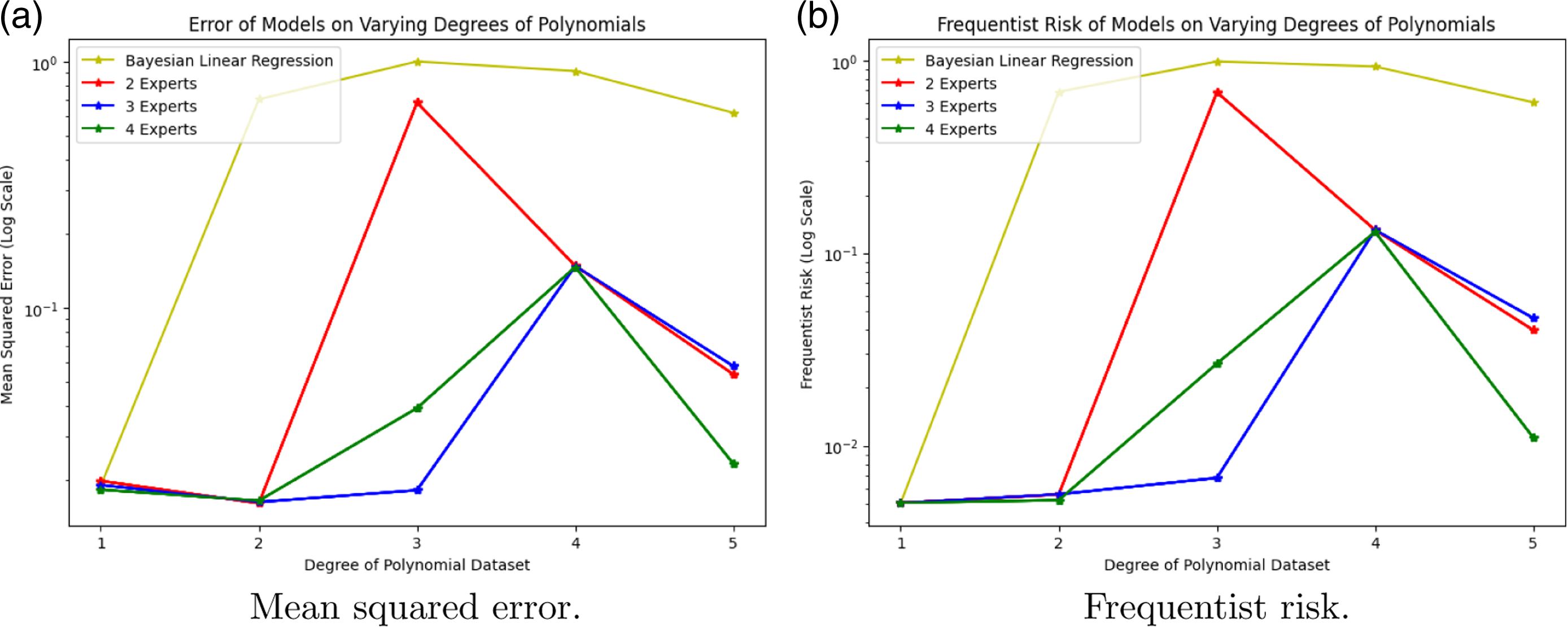


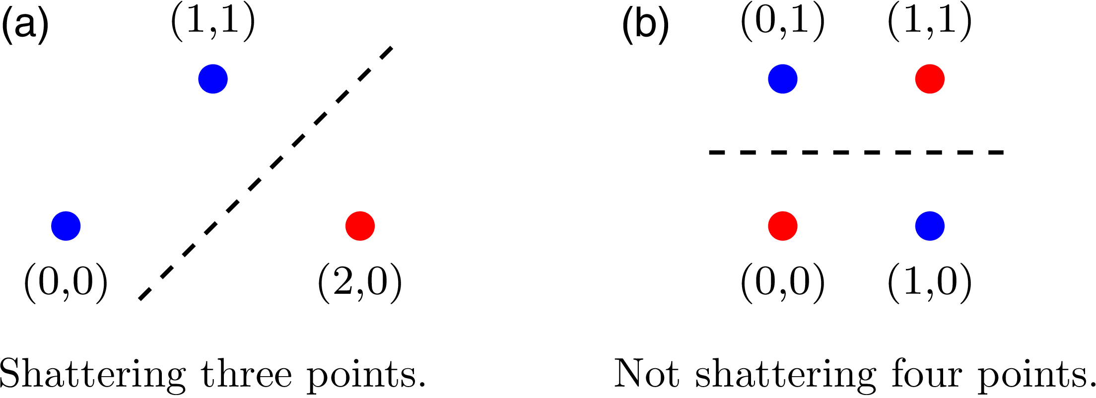
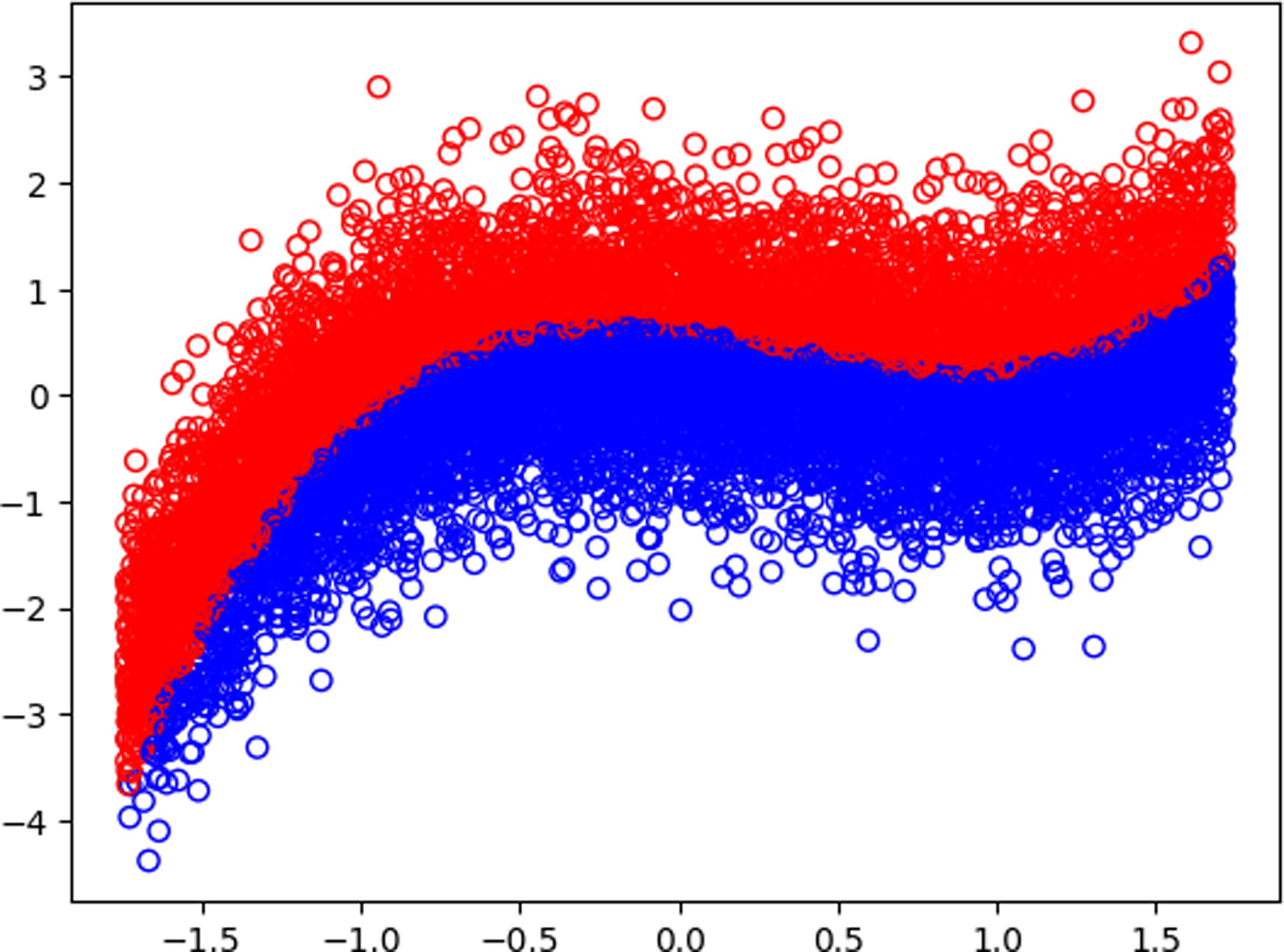


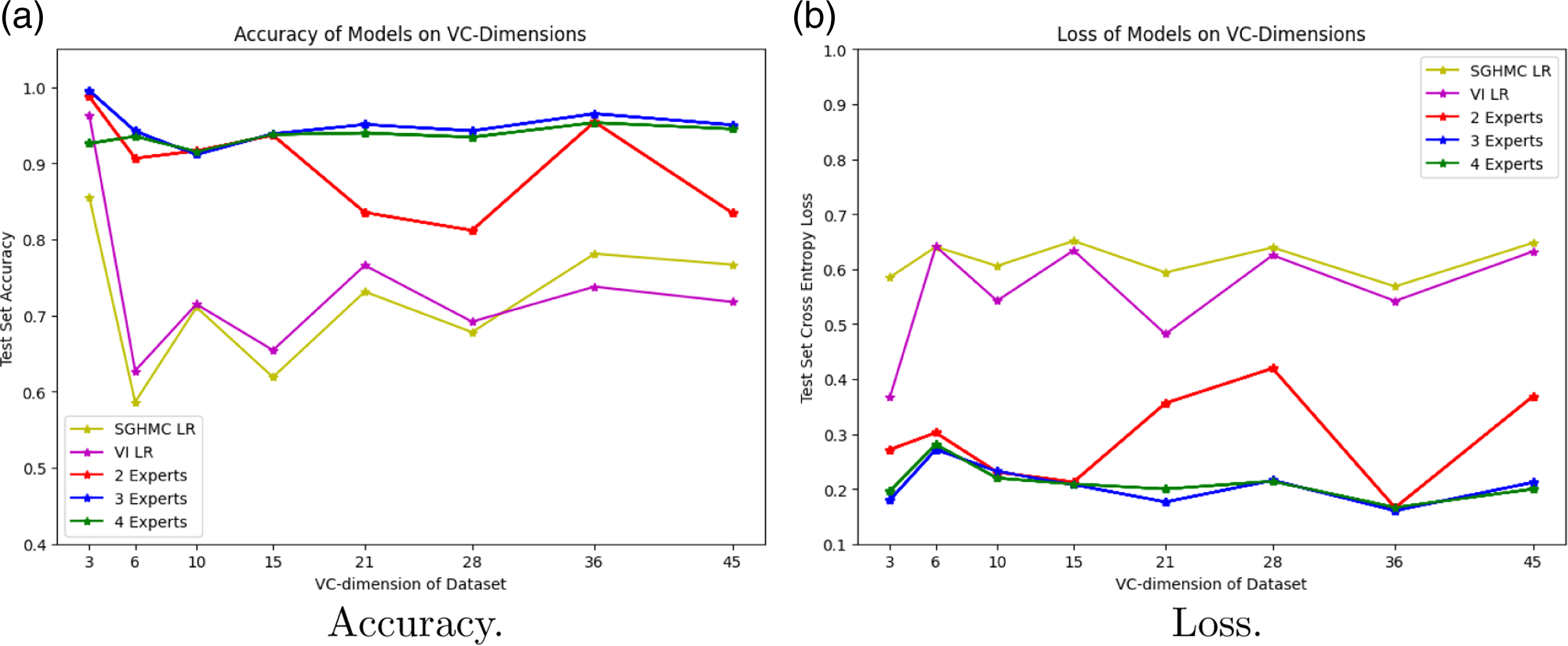


 Open access

