


1. Introduction
The dynamics of convective boundary layers (CBLs) that occur, for example, in mid-latitudes at midday conditions and over land, are governed by turbulent convection and shear-driven turbulence. On a scale of the order of the depth of CBLs (1–2 km), fluxes of momentum, heat and moisture are carried vertically by these turbulent motions (Garratt Reference Garratt1994; Wyngaard Reference Wyngaard2010). The two physical quantities that are directly linked to this vertical transport are vertical velocity and buoyancy of a fluid parcel. They are positively correlated in most of the CBL to form updrafts and downdrafts (see figure 1), which are mainly buoyant and non-buoyant, respectively (Schumann & Moeng Reference Schumann and Moeng1991).
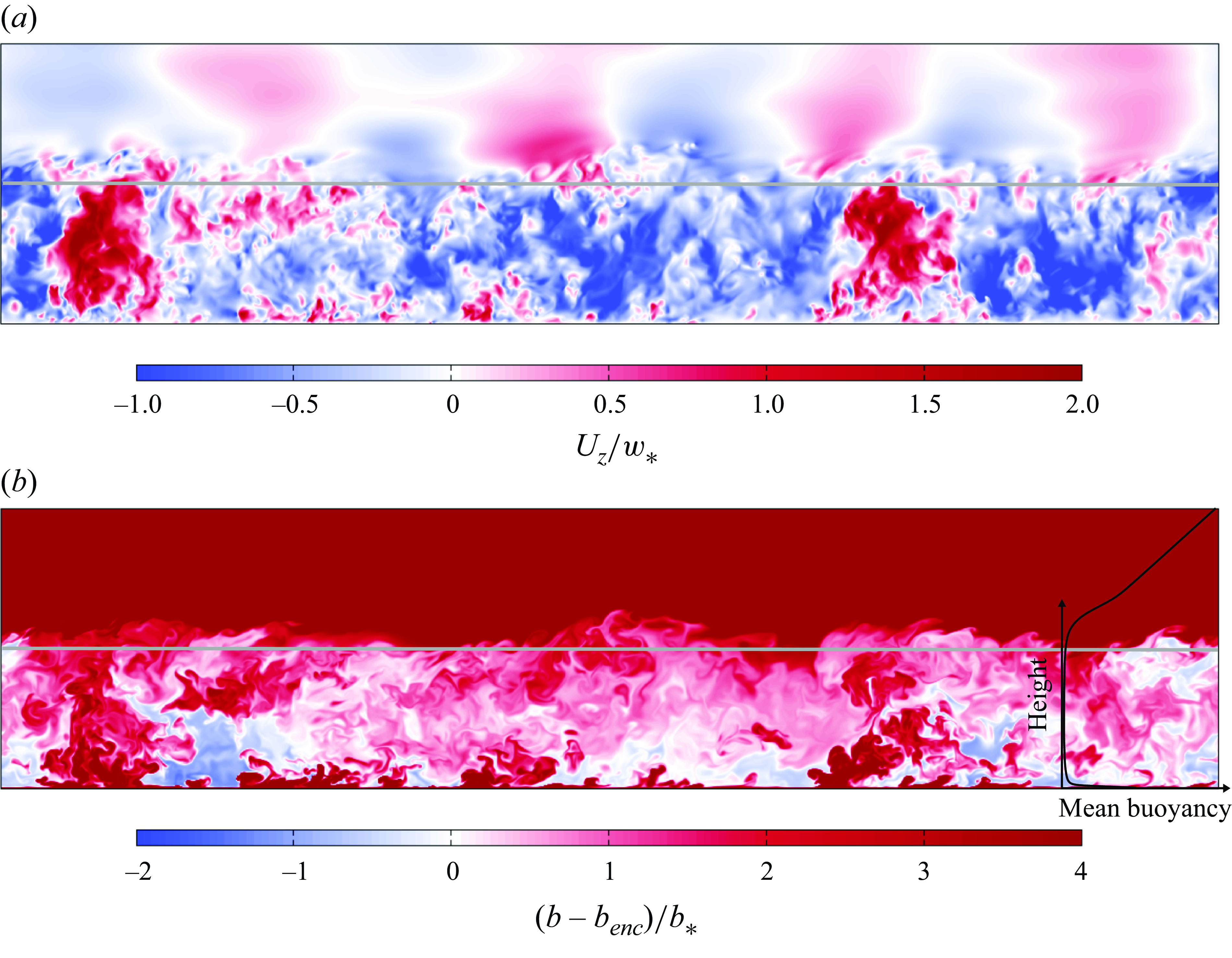
Visualisation of (a) the vertical velocity and (b) the buoyancy fields of a CBL studied in our analysis. The height of the atmospheric boundary layer $z_{{enc}}$
is indicated by the grey lines. The visualisation corresponds to the case
$z_{{enc}}$
is indicated by the grey lines. The visualisation corresponds to the case $Fr_0 = 20$
and
$Fr_0 = 20$
and ${\textit {Re}}_0 = 42$
at the time corresponding to
${\textit {Re}}_0 = 42$
at the time corresponding to $z_{{enc}}/L_0 \approx 26$
from table 1.
$z_{{enc}}/L_0 \approx 26$
from table 1.
The statistical analysis of CBLs has a long history. While early works tended to describe CBL mean profiles, structure and depth approximately similarly to an Ekman layer (for a review, see LeMone et al. Reference LeMone2019), seminal work by Deardorff (Reference Deardorff1970b, 1974a) showed that thermodynamic variables are the main indicators of CBL depth. During the same decade, due to new measurement capabilities, the picture of a well-mixed layer with near-constant values emerged (Clarke et al. Reference Clarke, Dyer, Brook, Reid and Troup1971; Kaimal et al. Reference Kaimal, Wyngaard, Haugen, Coté, Izumi, Caughey and Readings1976).
At the same time, Deardorff (Reference Deardorff1970b, Reference Deardorff1972, Reference Deardorff1974a ,Reference Deardorff b ) proved the validity of a so-called mixed layer scaling by characterising the CBL depth. He also investigated the structure of velocity and temperature fields under weak convective conditions. He showed that these fields are organised in coherent structures closely aligned with the mean wind direction near the ground, while for more convective conditions, updrafts are organised in open cells. The organisation of velocity and temperature as well as of velocity and buoyancy fields became a central topic in the study of CBLs through the work of Grossman (Reference Grossman1982) and Schmidt & Schumann (Reference Schmidt and Schumann1989). Moeng & Sullivan (Reference Moeng and Sullivan1994) and Fedorovich et al. (Reference Fedorovich, Conzemius, Esau, Chow, Lewellen, Moeng, Pino, Sullivan and Vila-Guerau de Arellano2004a ) also investigated the velocity field by considering not only its organisation, but also the vertical profiles of the second- and third-order moments, and the turbulence kinetic energy budget. In addition, Conzemius & Fedorovich (Reference Conzemius and Fedorovich2006) investigated the effects of shear on the tip and surface of a CBL. There is also a long history of parametrisation schemes of the CBL for weather and climate models (Baklanov et al. Reference Baklanov, Grisogono, Bornstein, Mahrt, Zilitinkevich, Taylor, Larsen, Rotach and Fernando2011; Edwards et al. Reference Edwards, Beljaars, Holtslag and Lock2020). Nonetheless, understanding and characterising the structure of CBLs in terms of a comprehensive analysis of what regulates the distribution of convective vertical motion remains a challenge.
For example, it is still crucial to know how the vertical velocity is distributed between updrafts and downdrafts to correctly represent vertical transport and its link to different atmospheric processes and models (Siebesma et al. Reference Siebesma, Soares and Teixeira2007; Suselj et al. Reference Suselj, Kurowski and Teixeira2019; Witte et al. Reference Witte, Herrington, Teixeira, Kurowski, Chinita, Storer, Suselj, Matheou and Bacmeister2022). In cloud processes, the updraft speed plays a key role in the formation of cloud droplets (Donner et al. Reference Donner, O’Brien, Rieger, Vogel and Cooke2016; Fitch Reference Fitch2019). In weather forecasting and boundary layer parametrisation, the simulated intensity and structure of hurricanes depend on the various methods used for representing turbulent fluxes and vertical mixing (Kepert Reference Kepert2012; Tang et al. Reference Tang, Zhang, Kieu and Marks2018). For the development of pollution dispersion models, it is important to correctly characterise the vertical structure of the wind (Bærentsen & Berkowicz Reference Bærentsen and Berkowicz1984; Quintarelli Reference Quintarelli1990; Weil et al. Reference Weil, Corio and Brower1997; Cimorelli et al. Reference Cimorelli, Perry, Venkatram, Weil, Paine, Wilson, Lee, Peters and Brode2005). When the updrafts enter the free atmosphere, they create an intermittent pattern of turbulent and non-turbulent regions, and this intermittency strongly affects the properties of the entrainment zone (Sullivan et al. Reference Sullivan, Moeng, Stevens, Lenschow and Mayor1998; Fedorovich et al. Reference Fedorovich, Conzemius and Mironov2004b ; Fodor et al. Reference Fodor, Mellado and Haghshenas2022). Large-scale updrafts and downdrafts are also responsible for deviations from the Monin–Obukhov similarity theory (e.g. Li et al. Reference Li, Gentine, Mellado and McColl2018; Fodor et al. Reference Fodor, Mellado and Wilczek2019; Salesky & Anderson Reference Salesky and Anderson2020), which assumes that within the boundary layer, all flow characteristics near the surface are solely determined by the friction velocity, surface buoyancy flux, and distance from the ground (Monin & Obukhov Reference Monin and Obukhov1954).
Here, we contribute to this line of research and investigate vertical velocity and buoyancy fields in CBLs for different conditions of surface heating, wind and buoyancy stratification by combining probability density function (PDF) methods and direct numerical simulations (DNS). The PDFs of these two fields feature non-trivial, height-dependent shapes. For example, the PDF of the vertical velocity features a negative mode (Wyngaard Reference Wyngaard2010; Berg et al. Reference Berg, Newsom and Turner2017). The mean vertical velocity, i.e. the first moment of the PDF of vertical velocity in boundary layers, including CBLs, is close to zero, whereas the normalised third moment, or skewness, in CBLs is positive and increases with height (Moeng & Rotunno Reference Moeng and Rotunno1990; Wyngaard Reference Wyngaard2010). This characteristic shape of the PDF for vertical velocity contains information about the structure of the CBL and its updrafts and downdrafts. Understanding how the PDFs for vertical velocity and for buoyancy evolve and behave along the depth of CBLs allows us to characterise the relevant statistics of these two quantities, enabling statistical insights into the structure of CBLs.
Evolution equations for PDFs can be derived from the equations of motion; see e.g. Lundgren (Reference Lundgren1967), Monin (Reference Monin1967)and Novikov (Reference Novikov1967). In the framework of so-called PDF methods popularised by Pope (Reference Pope1981, Reference Pope1985), this approach has been used successfully for statistical modelling. Combined with DNS data, the approach can be used to investigate the connection between turbulent dynamics and statistics; see e.g. Friedrich et al. (Reference Friedrich, Daitche, Kamps, Lülff, Voßkuhle and Wilczek2012) for a review. Lülff et al. (Reference Lülff, Wilczek and Friedrich2011, Reference Lülff, Wilczek, Stevens, Friedrich and Lohse2015) used such a combination of PDF methods and DNS data to study the PDFs of temperature and velocity in Rayleigh–Bénard convection (RBC) cells. In the work presented here, we use the same approach to understand and characterise the PDFs of buoyancy and velocity in a CBL, which is also convectively driven but without the top-down symmetry present in RBC. Thus this work will also allow us to understand how the results are different from those of RBC.
This top-down asymmetry intrinsic to CBLs is known to generate strong updrafts that occupy a small horizontal area and that are surrounded by downdraft regions with smaller velocities that occupy larger horizontal areas (Deardorff Reference Deardorff1972); furthermore, as height increases, the updrafts become stronger and narrower. This height-dependent change suggests a mass flux between updrafts and downdrafts. In fact, the concept of mass flux in CBLs has its roots in the cloud modelling community in which vertical turbulent transfer in CBLs is parametrised by assuming a two-stream system governed by an upward-moving stream and a downward-moving one (Chatfield & Brost Reference Chatfield and Brost1987; Siebesma et al. Reference Siebesma, Soares and Teixeira2007; Gentine et al. Reference Gentine, Betts, Lintner, Findell, Van Heerwaarden, Tzella and d’Andrea2013; Fitch Reference Fitch2019; Suselj et al. Reference Suselj, Kurowski and Teixeira2019; Witte et al. Reference Witte, Herrington, Teixeira, Kurowski, Chinita, Storer, Suselj, Matheou and Bacmeister2022). By extending our PDF analysis to the study of updrafts and downdrafts, we analyse their area fraction, and derive an equation that allows us to characterise the dynamical nature of the mass flux.
The statistical analysis of CBLs in this work builds on the PDF method approach, and focuses on single-time, single-point PDFs for vertical velocity and buoyancy. We derive an exact evolution equation for the joint PDF of vertical velocity and buoyancy, then project it onto the evolution equation of the marginal PDFs for the vertical velocity and the buoyancy. These equations feature unclosed terms in the form of conditional means of buoyancy, the negative of the vertical pressure gradient (vertical pressure gradient force from now on), viscous diffusion, vertical velocity, heat diffusion and vertical advection, which we determine from DNS of CBLs for different atmospheric conditions. By using the method of characteristics, we investigated how these effects jointly determine the average evolution of a fluid element in CBLs, and how this relates to the evolution of the PDF as a function of height.
This paper is structured as follows. In § 2, we describe the CBLs analysed in this study, as well as their governing equations and the numerical methods that we use to simulate them. In § 3, we recount the statistical analysis by presenting a detailed account of PDF methods and the method of characteristics. There, we analyse separately vertical velocity and buoyancy, including an analysis of the first moments of their PDFs, and a study of their area fractions. Finally, in § 4, we discuss and interpret the findings.
2. Description of the CBL
We study idealised CBLs for conditions that are characteristic for midday and over land. We model them as cloud-free, barotropic CBLs that develop over a homogeneous, flat and aerodynamically smooth surface, and that penetrate into a free atmosphere with a constant buoyancy gradient. Despite its simplicity compared to real atmospheric conditions, this idealised configuration has provided notable insight into the CBL, for instance, regarding the relevance of the convective velocity scale (Deardorff Reference Deardorff1970a) and the cellular and roll-like organisation of the flow (Schmidt & Schumann Reference Schmidt and Schumann1989; Moeng & Sullivan Reference Moeng and Sullivan1994), as well as entrainment properties (Sullivan et al. Reference Sullivan, Moeng, Stevens, Lenschow and Mayor1998; Fedorovich et al. Reference Fedorovich, Conzemius, Esau, Chow, Lewellen, Moeng, Pino, Sullivan and Vila-Guerau de Arellano2004a ).
For the considered cases, all within the limit of zero Coriolis parameter following work by Haghshenas & Mellado (Reference Haghshenas and Mellado2019), convection is forced and maintained by a constant buoyancy flux at the surface. Shear is imposed by a mean wind velocity. Details of the formulation and the simulations are provided by Haghshenas & Mellado (Reference Haghshenas and Mellado2019), but we summarise them here for convenience.
2.1. Governing equations
The CBL that we consider is governed by the conservation equations for mass, momentum, and buoyancy following the Oberbeck–Boussinesq approximation. They represent the CBL as an incompressible fluid by assuming that the density varies linearly with temperature with only small variations. The resulting set of coupled partial differential equations (PDEs) describes the evolution of velocity $\boldsymbol {U}$
and buoyancy
$\boldsymbol {U}$
and buoyancy $b$
in space and time (Stull Reference Stull1988):
$b$
in space and time (Stull Reference Stull1988):
 \begin{align} {\boldsymbol \nabla} \boldsymbol \cdot \boldsymbol {U}(\boldsymbol {x},t) = 0, \qquad\qquad\qquad\qquad\qquad\qquad\end{align}
 \begin{align} \frac {\partial }{\partial t} \boldsymbol {U}( \boldsymbol {x},t) +\boldsymbol {U} ( \boldsymbol {x},t) \boldsymbol \cdot {\boldsymbol \nabla } \boldsymbol {U}( \boldsymbol {x},t) = \nu\, \nabla ^2 \boldsymbol {U}(\boldsymbol {x},t) - \nabla p( \boldsymbol {x},t) +b ( \boldsymbol {x},t)\, \boldsymbol {e}_z, \end{align}
 \begin{align} \frac {\partial }{\partial t} b ( \boldsymbol {x},t) +\boldsymbol {U} ( \boldsymbol {x},t) {\boldsymbol \cdot } {\boldsymbol \nabla } b( \boldsymbol {x},t) = \kappa _b\, \nabla ^2 b(\boldsymbol {x},t). \qquad\qquad\quad\end{align}
Here, $\boldsymbol {U} ( \boldsymbol {x}, t )$
is the velocity field with components
$\boldsymbol {U} ( \boldsymbol {x}, t )$
is the velocity field with components $(U_x,U_y,U_z)$
in the streamwise, spanwise and normal directions, respectively; it depends on the spatial position
$(U_x,U_y,U_z)$
in the streamwise, spanwise and normal directions, respectively; it depends on the spatial position $\boldsymbol {x} = (x, y, z)$
and on time
$\boldsymbol {x} = (x, y, z)$
and on time $t$
. Also,
$t$
. Also, $\boldsymbol {e}_z = (0,0,1)$
is the unit vector in the vertical direction, and
$\boldsymbol {e}_z = (0,0,1)$
is the unit vector in the vertical direction, and $p$
is the kinematic pressure, i.e. the pressure divided by a constant reference density. The buoyancy
$p$
is the kinematic pressure, i.e. the pressure divided by a constant reference density. The buoyancy $b$
is linearly related to the virtual potential temperature
$b$
is linearly related to the virtual potential temperature $\theta _\nu$
as
$\theta _\nu$
as
 \begin{equation} b \approx g \left ( \frac {\theta _\nu - \theta _{\nu, 0}}{\theta _{\nu, 0}} \right )\!, \end{equation}
where $\theta _{\nu, 0}$
is a constant reference value at the surface, and
$\theta _{\nu, 0}$
is a constant reference value at the surface, and $g$
is the gravitational acceleration. Using a constant reference value
$g$
is the gravitational acceleration. Using a constant reference value $\theta _{\nu, 0}$
instead of the mean potential temperature at each height and time simplifies the evolution equation for
$\theta _{\nu, 0}$
instead of the mean potential temperature at each height and time simplifies the evolution equation for $b$
and the analysis (Garcia & Mellado Reference Garcia and Mellado2014; Haghshenas & Mellado Reference Haghshenas and Mellado2019). The kinematic molecular viscosity and thermal diffusivity are denoted by
$b$
and the analysis (Garcia & Mellado Reference Garcia and Mellado2014; Haghshenas & Mellado Reference Haghshenas and Mellado2019). The kinematic molecular viscosity and thermal diffusivity are denoted by $\nu$
and
$\nu$
and $\kappa _b$
, respectively.
$\kappa _b$
, respectively.
For the bottom boundary, we supplement these equations with impermeable, no-slip boundary conditions for velocity, and Neumann boundary conditions for buoyancy, $\partial _zb = -B_0/\kappa _b$
. Such conditions represent a CBL with a flat, smooth surface, forced by a constant and homogeneous surface buoyancy flux
$\partial _zb = -B_0/\kappa _b$
. Such conditions represent a CBL with a flat, smooth surface, forced by a constant and homogeneous surface buoyancy flux $B_0$
. At the top, impermeable, free-slip and Neumann boundary conditions are applied for velocity and buoyancy, respectively, with
$B_0$
. At the top, impermeable, free-slip and Neumann boundary conditions are applied for velocity and buoyancy, respectively, with $\partial _zb = N_0^2$
to maintain fixed constant fluxes. Here,
$\partial _zb = N_0^2$
to maintain fixed constant fluxes. Here, $N_0$
is the Brunt–Väisälä frequency, or buoyancy frequency. For the streamwise and spanwise directions, periodic boundary conditions are applied. Furthermore, when a shear-driven CBL is considered, an initial mean wind velocity
$N_0$
is the Brunt–Väisälä frequency, or buoyancy frequency. For the streamwise and spanwise directions, periodic boundary conditions are applied. Furthermore, when a shear-driven CBL is considered, an initial mean wind velocity $U_0$
is imposed in the streamwise direction. For barotropic boundary layers such as the one considered here,
$U_0$
is imposed in the streamwise direction. For barotropic boundary layers such as the one considered here, $U_0$
is constant with height in the free atmosphere. Finally, the initial buoyancy field increases linearly with height as
$U_0$
is constant with height in the free atmosphere. Finally, the initial buoyancy field increases linearly with height as $N_0^2$
. The mean vertical profile of buoyancy, as shown in figure 1, establishes the structure of the CBL, with distinct changes across its three main regions: the surface layer, mixed layer and entrainment zone. Near the surface, buoyancy decreases, influenced by surface properties. In the mixed layer, turbulent mixing results in a relatively uniform buoyancy profile. At the entrainment zone, buoyancy increases rapidly as more buoyant, stratified air from the free atmosphere interacts with less buoyant air from the mixed layer. This transition creates a buoyancy gradient, with the one-way process of entrainment allowing the mixed layer to grow upwards as more buoyant air is mixed downwards into the boundary layer.
$N_0^2$
. The mean vertical profile of buoyancy, as shown in figure 1, establishes the structure of the CBL, with distinct changes across its three main regions: the surface layer, mixed layer and entrainment zone. Near the surface, buoyancy decreases, influenced by surface properties. In the mixed layer, turbulent mixing results in a relatively uniform buoyancy profile. At the entrainment zone, buoyancy increases rapidly as more buoyant, stratified air from the free atmosphere interacts with less buoyant air from the mixed layer. This transition creates a buoyancy gradient, with the one-way process of entrainment allowing the mixed layer to grow upwards as more buoyant air is mixed downwards into the boundary layer.
2.2. Control parameters and dimensional analysis
The CBL described in the previous subsection can be fully characterised by the control parameters $\{ \nu, \kappa _b, B_0, N_0, U_0 \}$
. Based on these five control parameters, one can define three non-dimensional parameters that characterise the full system. In this study, we analyse the impact of shear over the statistical behaviour of CBLs, and compare it in particular to the shear-free case (
$\{ \nu, \kappa _b, B_0, N_0, U_0 \}$
. Based on these five control parameters, one can define three non-dimensional parameters that characterise the full system. In this study, we analyse the impact of shear over the statistical behaviour of CBLs, and compare it in particular to the shear-free case ( $U_0 =0$
). Therefore, we follow previous work by Haghshenas & Mellado (Reference Haghshenas and Mellado2019), and we choose
$U_0 =0$
). Therefore, we follow previous work by Haghshenas & Mellado (Reference Haghshenas and Mellado2019), and we choose $B_0$
and
$B_0$
and $N_0$
to non-dimensionalise the system.
$N_0$
to non-dimensionalise the system.
In particular, $N_0^{-1}$
is the reference time scale, and the Ozmidov length
$N_0^{-1}$
is the reference time scale, and the Ozmidov length
 \begin{equation} L_0 \equiv \left ( \frac {B_0}{N_0^3} \right )^{\frac{1}{2}} \end{equation}
is the reference length scale. The latter represents the size of the larger turbulent motions that are unaffected by a background stratification induced by $N_0^2$
, and it characterises the entrainment zone thickness. Furthermore, we consider the reference buoyancy Reynolds number
$N_0^2$
, and it characterises the entrainment zone thickness. Furthermore, we consider the reference buoyancy Reynolds number
 \begin{equation} {\textit {Re}}_0 \equiv \frac {B_0}{\nu N_0 ^2}, \end{equation}
as well as the reference Froude number
 \begin{equation} Fr_0 \equiv \frac {U_0}{(B_0 L_0)^{\frac{1}{3}}}. \end{equation}
On account of the statistical homogeneity in streamwise and spanwise directions, the single-point statistical properties of the system are functions of only height and time $(z,t)$
. Of particular relevance for our analysis is the height dependence. We non-dimensionalise
$(z,t)$
. Of particular relevance for our analysis is the height dependence. We non-dimensionalise $z$
as
$z$
as $\hat {z} = z/z_{{enc}}$
with the encroachment length scale
$\hat {z} = z/z_{{enc}}$
with the encroachment length scale $z_{{enc}}$
:
$z_{{enc}}$
:
 \begin{equation} z_{{enc}}(t)\equiv \left [ 2 N_0^{-2} \int _0^{z_\infty } [ \langle b \rangle (z,t) - N_0^2 z ] {\rm d}z \right ]^{\frac{1}{2}}. \end{equation}
The upper limit of the integral, $z_\infty$
, is located far enough above the encroachment zone and well into the free atmosphere; this ensures that the integral is independent of
$z_\infty$
, is located far enough above the encroachment zone and well into the free atmosphere; this ensures that the integral is independent of $z_\infty$
. Here, angle brackets represent an average over the horizontal directions. The encroachment length scale provides a measure of the depth of the CBL and its growth over time in both sheared (Haghshenas & Mellado Reference Haghshenas and Mellado2019) and shear-free (Carson & Smith Reference Carson and Smith1975) CBLs. Integrating the evolution equation for the mean buoyancy vertically, one can obtain the following relationship (Haghshenas & Mellado Reference Haghshenas and Mellado2019)
$z_\infty$
. Here, angle brackets represent an average over the horizontal directions. The encroachment length scale provides a measure of the depth of the CBL and its growth over time in both sheared (Haghshenas & Mellado Reference Haghshenas and Mellado2019) and shear-free (Carson & Smith Reference Carson and Smith1975) CBLs. Integrating the evolution equation for the mean buoyancy vertically, one can obtain the following relationship (Haghshenas & Mellado Reference Haghshenas and Mellado2019)
 \begin{equation} \frac{z_{enc}}{L_0} = [2(1 + Re_0^{-1} )N_0 (t - t_0 )]^{\frac{1}{2}} \approx (2 N_0 t)^{\frac{1}{2}} , \end{equation}
where $t_0$
is a constant of integration and the approximation is valid for large enough Reynolds numbers and large enough times. We will use this approximate relationship between the encroachment length and time in the following sections.
$t_0$
is a constant of integration and the approximation is valid for large enough Reynolds numbers and large enough times. We will use this approximate relationship between the encroachment length and time in the following sections.
2.3. The DNS
The simulations employ a finite-difference method with Cartesian coordinates and a structured grid. A sixth-order spectral-like compact scheme is used to evaluate the spatial derivatives (Lele Reference Lele1992); a fourth-order low-storage Runge–Kutta scheme is used to advance the fields in time (Carpenter & Kennedy Reference Carpenter and Kennedy1994). The incompressibility of the fluid is imposed by a Fourier decomposition of the Poisson equation for the pressure in the horizontal directions (Mellado & Ansorge Reference Mellado and Ansorge2012).
A non-uniform grid is used in the vertical direction near the surface and above the turbulent boundary layer in the free atmosphere. Near the surface, the vertical grid is refined to provide the required higher resolution. In the free atmosphere, well above the turbulent boundary layer, the vertical grid is coarsened to move the top of the computational domain far away from the boundary layer and thus reduce its spurious effects.
The grid in the horizontal directions is uniform and isotropic, except for the case $Fr_0 = 20$
. The anisotropic grid in horizontal directions when
$Fr_0 = 20$
. The anisotropic grid in horizontal directions when $Fr_0 = 20$
serves to save computational time while still meeting the necessary resolution constraints. As indicated before, further details about the grid and simulation set-up can be found in Haghshenas & Mellado (Reference Haghshenas and Mellado2019). The specific grid choice of some simulations varies slightly from those outlined in Haghshenas & Mellado (Reference Haghshenas and Mellado2019) due to the simulations being performed on a different cluster. Table 1 shows the grid size for the simulations that we analyse.
$Fr_0 = 20$
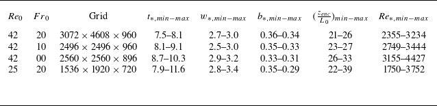
serves to save computational time while still meeting the necessary resolution constraints. As indicated before, further details about the grid and simulation set-up can be found in Haghshenas & Mellado (Reference Haghshenas and Mellado2019). The specific grid choice of some simulations varies slightly from those outlined in Haghshenas & Mellado (Reference Haghshenas and Mellado2019) due to the simulations being performed on a different cluster. Table 1 shows the grid size for the simulations that we analyse.
Simulation parameters for the CBLs analysed in this study. Columns 4–6 show the values of the convective scales at the beginning of the quasi-steady regime, and at the final time that we considered. Column 3 shows the number of grid points in the streamwise, spanwise and vertical directions, respectively. Values are non-dimensionalised with $B_0$
and
$B_0$
and $N_0$
. The convective Reynolds number is defined as
$N_0$
. The convective Reynolds number is defined as ${\textit {Re}}_*=z_{{enc}}w_*/\nu$
.
${\textit {Re}}_*=z_{{enc}}w_*/\nu$
.
2.4. Description of simulations and parameter space
Boundary layers in midday conditions and fair weather over land are typically characterised by the following values of the control parameters (Fedorovich et al. Reference Fedorovich, Conzemius and Mironov2004b
): surface buoyancy flux $B_0 \approx (0.3{-}1.0)\times 10^{-2}\,\text {m}^2\, \text {s}^{-3}$
, buoyancy frequency in the free atmosphere
$B_0 \approx (0.3{-}1.0)\times 10^{-2}\,\text {m}^2\, \text {s}^{-3}$
, buoyancy frequency in the free atmosphere $N_0 \approx (0.6{-}1.8)\times 10^{-2}\,\text {s}^{-1}$
, and wind velocity in the free troposphere
$N_0 \approx (0.6{-}1.8)\times 10^{-2}\,\text {s}^{-1}$
, and wind velocity in the free troposphere $U_0 = 0{-}15\, \text {m}\,{\rm s}^{-1}$
. Under those conditions, one finds
$U_0 = 0{-}15\, \text {m}\,{\rm s}^{-1}$
. Under those conditions, one finds $L_0 \approx 20{-}200\, \text {m}$
and
$L_0 \approx 20{-}200\, \text {m}$
and $Fr_0 \approx 0{-}35$
. Typical values of the CBL height are
$Fr_0 \approx 0{-}35$
. Typical values of the CBL height are $z_{{enc}} \approx 500{-}2000\,\text {m}$
, and typical values of the normalised height are
$z_{{enc}} \approx 500{-}2000\,\text {m}$
, and typical values of the normalised height are $z_{{enc}}/L_0\approx 5{-}50$
. Furthermore, assuming
$z_{{enc}}/L_0\approx 5{-}50$
. Furthermore, assuming $\kappa _b = 2.1 \times 10^{-5}\,\text {m}^2\,\text {s}^{-1}$
and
$\kappa _b = 2.1 \times 10^{-5}\,\text {m}^2\,\text {s}^{-1}$
and $\nu = 1.5 \times 10^{-5}\, \text {m}^2\,\text {s}^{-1}$
results in
$\nu = 1.5 \times 10^{-5}\, \text {m}^2\,\text {s}^{-1}$
results in ${\textit {Re}}_0 \approx 6 \times 10^5{-}2 \times 10^7$
and a molecular Prandtl number
${\textit {Re}}_0 \approx 6 \times 10^5{-}2 \times 10^7$
and a molecular Prandtl number ${\textit {Pr}}=\nu /\kappa _b \approx 0.7$
.
${\textit {Pr}}=\nu /\kappa _b \approx 0.7$
.
In this work, we fix ${\textit {Pr}} = 1$
and study cases for three different Froude numbers,
${\textit {Pr}} = 1$
and study cases for three different Froude numbers, $Fr_0 = 0, \, 10, \, 20$
. Here,
$Fr_0 = 0, \, 10, \, 20$
. Here, $Fr_0 = 0$
represents a zero-wind boundary layer and
$Fr_0 = 0$
represents a zero-wind boundary layer and $Fr_0 = 20$
a strong-wind boundary layer, when wind-shear effects are of order one.
$Fr_0 = 20$
a strong-wind boundary layer, when wind-shear effects are of order one.
Regarding the reference Reynolds number, large-eddy simulations and DNS cannot reach atmospheric values. Such simulation studies rely on the observation that some relevant properties become increasingly independent of the Reynolds number once it reaches a critical value (Dimotakis Reference Dimotakis2000), which we are reaching for relevant atmospheric cases such as the CBL (Garcia & Mellado Reference Garcia and Mellado2014; Haghshenas & Mellado Reference Haghshenas and Mellado2019; Mellado et al. Reference Mellado, Puche and van Heerwaarden2017). Compared to large-eddy simulations, DNS have typically a higher computational cost, but the advantage is that they remove the uncertainty associated with subgrid scale models, facilitating the analysis and interpretation of results. To explore the potential sensitivity of our results to the Reynolds number, the main analysis is based on ${\textit {Re}}_0 \approx 42$
, and the results are compared to the case with
${\textit {Re}}_0 \approx 42$
, and the results are compared to the case with ${\textit {Re}}_0 \approx 25$
.
${\textit {Re}}_0 \approx 25$
.
The size of the computational domain is $215L_0 \times 215L_0 \times 130L_0$
, where at
$215L_0 \times 215L_0 \times 130L_0$
, where at $z_{{enc}}/L_0 \approx 35$
, the CBL covers
$z_{{enc}}/L_0 \approx 35$
, the CBL covers $30\,\%$
of it in the vertical direction.
$30\,\%$
of it in the vertical direction.
2.5. Convective scales and quasi-steady regime
For CBLs, a central length scale is the (time-dependent) encroachment height $z_{{enc}}$
. Key statistical quantities are expected to scale with
$z_{{enc}}$
. Key statistical quantities are expected to scale with $z_{{enc}}$
. For example, velocity fluctuations scale in magnitude with the convective velocity (Deardorff Reference Deardorff1970a; Berg et al. Reference Berg, Newsom and Turner2017)
$z_{{enc}}$
. For example, velocity fluctuations scale in magnitude with the convective velocity (Deardorff Reference Deardorff1970a; Berg et al. Reference Berg, Newsom and Turner2017)
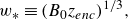 \begin{equation} w_* \equiv (B_0 z_{{enc}})^{1/3}, \end{equation}
and buoyancy fluctuations with the convective buoyancy
 \begin{equation} b_* \equiv \frac {B_0}{w_*}. \end{equation}
Furthermore, we define a convective time scale
 \begin{equation} t_* \equiv \dfrac {z_{{enc}}}{w_*}. \end{equation}
Note that $w_*$
,
$w_*$
, $b_*$
and
$b_*$
and $t_*$
depend on
$t_*$
depend on $z_{{enc}}$
. Similarly, central statistical quantities, such as the PDF of the vertical velocity
$z_{{enc}}$
. Similarly, central statistical quantities, such as the PDF of the vertical velocity $f(W)$
, buoyancy
$f(W)$
, buoyancy $f(\theta )$
, and the respective moments, are expected to become self-similar in their time evolution in the mixed layer when normalised in height with
$f(\theta )$
, and the respective moments, are expected to become self-similar in their time evolution in the mixed layer when normalised in height with $z_{{enc}}$
, and standardised with
$z_{{enc}}$
, and standardised with $w_*$
,
$w_*$
, $b_*$
, or a combination of them. This self-similar behaviour is achieved during the equilibrium, or quasi-steady entrainment regime. Garcia & Mellado (Reference Garcia and Mellado2014) and Haghshenas & Mellado (Reference Haghshenas and Mellado2019) showed that for shear-free and sheared CBLs that grow into a linearly stratified free atmosphere, the quasi-steady entrainment regime is achieved when
$b_*$
, or a combination of them. This self-similar behaviour is achieved during the equilibrium, or quasi-steady entrainment regime. Garcia & Mellado (Reference Garcia and Mellado2014) and Haghshenas & Mellado (Reference Haghshenas and Mellado2019) showed that for shear-free and sheared CBLs that grow into a linearly stratified free atmosphere, the quasi-steady entrainment regime is achieved when $z_{{enc}}/L_0 \approx 10$
and beyond.
$z_{{enc}}/L_0 \approx 10$
and beyond.
We consider only CBLs that have reached the quasi-steady regime, and scale all the vertical distributions and statistics of fluctuating velocity and buoyancy with $w_*$
,
$w_*$
, $b_*$
,
$b_*$
, $z_{{enc}}$
, or a combination of them; see Appendix A. These convective scales characterise the fluctuation fields in the mixed layer of the CBL (Wyngaard Reference Wyngaard2010), which is the region on which we want to focus here.
$z_{{enc}}$
, or a combination of them; see Appendix A. These convective scales characterise the fluctuation fields in the mixed layer of the CBL (Wyngaard Reference Wyngaard2010), which is the region on which we want to focus here.
Table 1 shows an overview of the CBLs that we analyse. We will focus on the case ${\textit {Re}}_0=42$
and
${\textit {Re}}_0=42$
and $Fr_0=20$
during the presentation of the results and the discussions, and will comment on the effects of Reynolds and Froude numbers as needed. As mentioned, we consider only CBLs that have reached the quasi-steady regime. The table shows the initial and final values of the convective scales in the regime that we analyse. When performing the statistical analysis, we considered the statistical homogeneity of the system in the horizontal directions, and replaced ensemble averages with spatial averages in the streamwise and spanwise directions. Furthermore, to improve the statistical convergence of our analysis, spatial horizontal averages are additionally averaged over four planes in the vertical direction and in time. Hence, when plotting the data, the curves indicate the running average within a time interval of the quasi-steady regime, and the shaded areas denote the range within two standard deviations from the presented average.
$Fr_0=20$
during the presentation of the results and the discussions, and will comment on the effects of Reynolds and Froude numbers as needed. As mentioned, we consider only CBLs that have reached the quasi-steady regime. The table shows the initial and final values of the convective scales in the regime that we analyse. When performing the statistical analysis, we considered the statistical homogeneity of the system in the horizontal directions, and replaced ensemble averages with spatial averages in the streamwise and spanwise directions. Furthermore, to improve the statistical convergence of our analysis, spatial horizontal averages are additionally averaged over four planes in the vertical direction and in time. Hence, when plotting the data, the curves indicate the running average within a time interval of the quasi-steady regime, and the shaded areas denote the range within two standard deviations from the presented average.
3. Statistical description of vertical velocity and buoyancy
We are interested primarily in the statistics of the vertical velocity and buoyancy fluctuations. Their single-point statistics can be captured comprehensively in terms of their PDFs $f(W;z,t)$
and
$f(W;z,t)$
and $f(\theta ;z,t)$
. Their joint PDF can be formally introduced as an ensemble average of the fine-grained distribution (Pope Reference Pope2000):
$f(\theta ;z,t)$
. Their joint PDF can be formally introduced as an ensemble average of the fine-grained distribution (Pope Reference Pope2000):
 \begin{equation} f(W,\theta ;z,t) = \langle \delta (U_z(\boldsymbol x,t)-W)\, \delta (b(\boldsymbol x,t)-\theta ) \rangle . \end{equation}
Here, $W$
is the sample-space variable corresponding to the vertical velocity realisation
$W$
is the sample-space variable corresponding to the vertical velocity realisation $U_z$
,
$U_z$
, $\theta$
is the sample-space variable corresponding to the buoyancy realisation
$\theta$
is the sample-space variable corresponding to the buoyancy realisation $b$
, and
$b$
, and $\delta$
is the Dirac delta function. Note that we have already assumed homogeneity in horizontal directions such that the PDF depends only on the vertical coordinate
$\delta$
is the Dirac delta function. Note that we have already assumed homogeneity in horizontal directions such that the PDF depends only on the vertical coordinate $z$
. Based on this definition, and using the equations of motion (2.1), we can derive an evolution equation for the joint PDF using PDF methods (Pope Reference Pope1981, Reference Pope1985, Reference Pope2000), which takes the form (see Appendix B)
$z$
. Based on this definition, and using the equations of motion (2.1), we can derive an evolution equation for the joint PDF using PDF methods (Pope Reference Pope1981, Reference Pope1985, Reference Pope2000), which takes the form (see Appendix B)
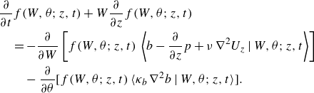 \begin{align} &\frac {\partial }{\partial t}f(W,\theta ;z,t) + W \frac {\partial }{\partial z} f(W,\theta ;z,t) \notag\\&\quad = - \frac {\partial }{\partial W} \left [ f(W,\theta ;z,t)\,\left \langle b - \frac {\partial }{\partial z} p + \nu\, \nabla ^2 U_z\, \Big|\, W, \theta ;z,t \right \rangle \right ]\nonumber \\ &\qquad- \frac {\partial }{\partial \theta } [ f(W,\theta ;z,t)\, \langle \kappa _b\, \nabla ^2 {b}\,|\,W, \theta ;z,t \rangle ]. \end{align}
Here, $\langle \ldots \,|\,W, \theta ;z,t \rangle$
are conditional averages conditioned on
$\langle \ldots \,|\,W, \theta ;z,t \rangle$
are conditional averages conditioned on $W$
and
$W$
and $\theta$
. Note that the conditional averages are functions of
$\theta$
. Note that the conditional averages are functions of $z$
and
$z$
and $t$
too. The PDF equation takes the form of a continuity equation for the probability density. The advection of the PDF represented by the terms of the left-hand side appear in closed form. The conditional averages on the right-hand side represent unclosed terms that can be obtained from our DNS data, and interpreted in terms of their physical meaning.
$t$
too. The PDF equation takes the form of a continuity equation for the probability density. The advection of the PDF represented by the terms of the left-hand side appear in closed form. The conditional averages on the right-hand side represent unclosed terms that can be obtained from our DNS data, and interpreted in terms of their physical meaning.
The PDF equation describes the evolution of all the relevant statistics of the system in space and time by considering the influence of the CBLs on its right-hand side. For example, knowing this PDF means that we also know its first moments, which are the mean vertical velocity and mean buoyancy, and the second moments, i.e. the Reynolds stresses and heat fluxes. As we demonstrate in Appendix C, the evolution equations of the mean velocity and the normal Reynolds stress can be obtained by first projecting (3.2) into the $W$
-space, then taking moments of the resulting equation. We expand on this in what follows.
$W$
-space, then taking moments of the resulting equation. We expand on this in what follows.
3.1. Vertical velocity
3.1.1. PDF equation
By integrating the equation for the joint PDF (3.2) over buoyancy, we obtain the equation that governs the evolution of the marginal PDF for vertical velocity only:
 \begin{align} \frac {\partial }{\partial t}f(W;z,t) + W \frac {\partial }{\partial z} f(W;z,t) = - \frac {\partial }{\partial W} \left [ f(W;z,t)\, \left \langle b - \frac {\partial }{\partial z} p + \nu\, \nabla ^2 U_z\, \Big |\, W;z,t\right \rangle \right ].\notag\\[3pt] \end{align}
In the quasi-steady regime of CBLs, velocity fluctuations in the mixed layer scale with the convective velocity $w_*$
(Deardorff Reference Deardorff1970a) as
$w_*$
(Deardorff Reference Deardorff1970a) as
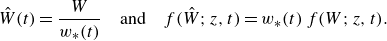 \begin{equation} \hat {W}(t) = \frac {W}{w_*(t)} \quad\text {and}\quad f(\hat {W};z,t) = w_*(t)\, f(W;z,t). \end{equation}
In Appendix A, we explicitly verify that for our DNS data under this scaling, the PDF $f(\hat {W};z,t)$
becomes quasi-stationary to a good approximation. Hence we can assume stationarity in our equation and consider
$f(\hat {W};z,t)$
becomes quasi-stationary to a good approximation. Hence we can assume stationarity in our equation and consider $\partial f(\hat {W};z,t)/\partial t \approx 0$
. In the following, we simplify the notation and drop the time dependence in the conditional averages and the PDF:
$\partial f(\hat {W};z,t)/\partial t \approx 0$
. In the following, we simplify the notation and drop the time dependence in the conditional averages and the PDF: $\langle \ldots \,|\,\hat {W};z,t \rangle =\langle \ldots \,|\,\hat {W};z \rangle$
. Thus we have converted (3.3) into a stationary equation, which we can further simplify by non-dimensionalising when multiplying the equation by
$\langle \ldots \,|\,\hat {W};z,t \rangle =\langle \ldots \,|\,\hat {W};z \rangle$
. Thus we have converted (3.3) into a stationary equation, which we can further simplify by non-dimensionalising when multiplying the equation by $z_{{enc}}$
. Consequently, (3.3) takes the form
$z_{{enc}}$
. Consequently, (3.3) takes the form
 \begin{equation} \hat {W} \frac {\partial }{\partial \hat {z}} f(\hat {W};\hat {z}) \approx - \frac {\partial }{\partial \hat {W}} \left [ f(\hat {W};\hat {z}) \left ( \,\left \langle \hat {b} - \frac {\partial }{\partial \hat {z}} \hat {p} + Re_*^{-1}\, \hat \nabla ^2 \hat {U}_z \,\Big |\, \hat {W};\hat {z}\right \rangle - \frac {1}{6\hat {t}} \hat {W} \right ) \right ], \end{equation}
where
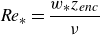 \begin{equation} {\textit {Re}}_* = \dfrac {w_* z_{{enc}}}{\nu } \end{equation}
is the convective Reynolds number, and
 \begin{equation} \hat {b} = b\dfrac {z_{{enc}}}{w_*^2}, \quad \frac {\partial }{\partial \hat {z}} = z_{{enc}} \frac {\partial }{\partial z}, \quad \hat {p} = p \frac {1}{w_*^2}, \quad \hat { \nabla } ^2 = z_{{enc}}^2\, \nabla ^2, \quad \hat {t} = \frac {t}{t_*}. \end{equation}
The right-hand side of (3.5) depends on the fluid element acceleration consisting of the conditional means of the buoyancy, the Laplacian of the vertical velocity, and the vertical gradient of pressure, and additionally, we obtain an extra term, from now on quasi-steady term, that originates from evaluating the time derivative in (3.3) using the time-dependent scaling (3.4). This term results from re-scaling the PDF to a quasi-steady form, and accounts for the temporal growth of the CBL due to the imposed constant heat flux and consequently of the convective scales. The temporal growth for which the quasi-steady term accounts is nonetheless insignificant within the quasi-steady regime that we analyse. We verified this with our DNS data, as we explain below.
Conditional averages of (a) buoyancy fluctuations conditioned on $\hat {W}$
, (b) vertical pressure gradient force fluctuations conditioned on
$\hat {W}$
, (b) vertical pressure gradient force fluctuations conditioned on $\hat {W}$
, and (c) the viscous term conditioned on
$\hat {W}$
, and (c) the viscous term conditioned on $\hat {W}$
. (d) Balance of the different terms in the conditional mean on the right-hand side of (3.5). The colour gradient indicates the different heights at which the averages are plotted. The CBL has
$\hat {W}$
. (d) Balance of the different terms in the conditional mean on the right-hand side of (3.5). The colour gradient indicates the different heights at which the averages are plotted. The CBL has ${\textit {Re}}_0 = 42$
and
${\textit {Re}}_0 = 42$
and $Fr_0 = 20$
.
$Fr_0 = 20$
.
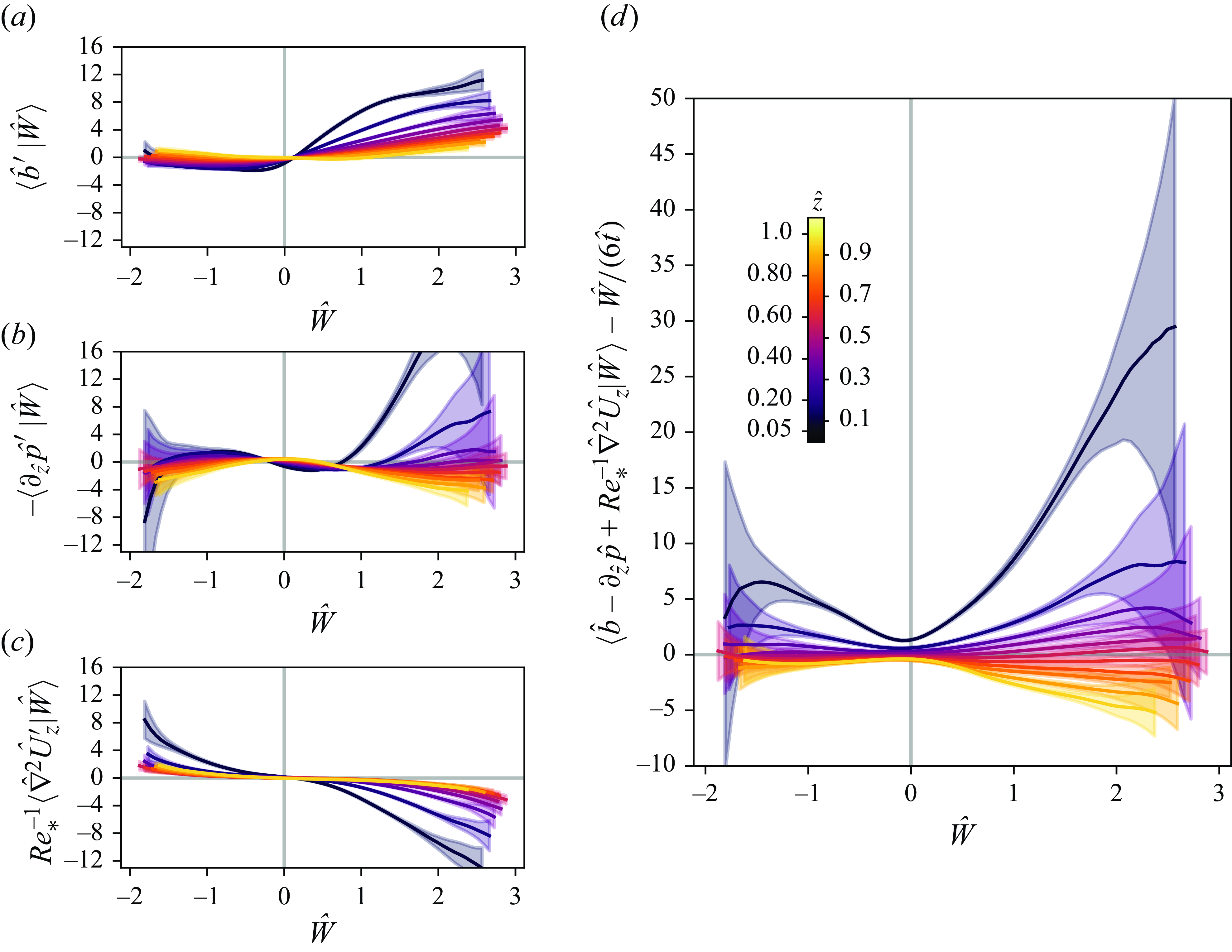
Using our CBL simulations, we can analyse the various unclosed terms in the PDF equation (3.5), giving insight into the conditional mean of fluid element acceleration, and in particular on its dependence with height.
Figure 2 shows the fluctuations of some of the individual terms, as well as the balance of the terms for the different heights indicated by the colour gradient. Note that whereas for the theoretical derivation of these equations we are assuming an ensemble average, for evaluating numerical data, this is replaced by a horizontal and time average. Figure 2(a–c) show only the fluctuations of the different terms since the mean of the buoyancy balances with the mean of the vertical pressure gradient force. The closed term in (3.5) proportional to $\hat {W}$
is not shown since it is, as expected, negligible in amplitude.
$\hat {W}$
is not shown since it is, as expected, negligible in amplitude.
From the figure, let us first analyse buoyancy fluctuations conditioned on $\hat {W}$
,
$\hat {W}$
, $\langle b' \,|\,\hat {W}\rangle$
. For positive values of
$\langle b' \,|\,\hat {W}\rangle$
. For positive values of $\hat {W}$
, buoyancy fluctuations tend to be positive, and to have larger magnitudes the closer they are to the surface. This is a direct consequence of the positive buoyancy flux that is constantly heating up the bottom boundary, thereby accelerating fluid parcels in contact with it and transferring energy into the system. Buoyancy fluctuations for negative values of
$\hat {W}$
, buoyancy fluctuations tend to be positive, and to have larger magnitudes the closer they are to the surface. This is a direct consequence of the positive buoyancy flux that is constantly heating up the bottom boundary, thereby accelerating fluid parcels in contact with it and transferring energy into the system. Buoyancy fluctuations for negative values of $\hat {W}$
behave differently. First, they have a smaller magnitude than those for positive velocities. Second, they do not necessarily tend to be all negative as one might expect; while they are indeed negative for the bottom region of the CBL, as the altitude increases, buoyancy fluctuations for negative velocities become positive. We interpret this tendency as a direct consequence of the entrainment of buoyant fluid parcels coming from the free atmosphere into the mixed layer of the CBL. We support this interpretation when analysing buoyancy fluctuations for a shear-free CBL (
$\hat {W}$
behave differently. First, they have a smaller magnitude than those for positive velocities. Second, they do not necessarily tend to be all negative as one might expect; while they are indeed negative for the bottom region of the CBL, as the altitude increases, buoyancy fluctuations for negative velocities become positive. We interpret this tendency as a direct consequence of the entrainment of buoyant fluid parcels coming from the free atmosphere into the mixed layer of the CBL. We support this interpretation when analysing buoyancy fluctuations for a shear-free CBL ( $Fr_0 = 0$
). For
$Fr_0 = 0$
). For $Fr_0 = 0$
, the amplitude of the buoyancy fluctuations for negative velocities close to the entrainment zone is, although still positive, smaller than for the cases
$Fr_0 = 0$
, the amplitude of the buoyancy fluctuations for negative velocities close to the entrainment zone is, although still positive, smaller than for the cases $Fr_0 = 10$
and
$Fr_0 = 10$
and $Fr_0 = 20$
(not shown). This is consistent with the fact that in shear-free CBLs, the absence of wind shear reduces the entrainment rate, meaning that less-buoyant parcels of air from the free atmosphere are entrained back into the mixed layer (e.g. Fedorovich et al. Reference Fedorovich, Conzemius, Esau, Chow, Lewellen, Moeng, Pino, Sullivan and Vila-Guerau de Arellano2004a
; Fodor et al. Reference Fodor, Mellado and Haghshenas2022). Note also that the buoyancy profiles lack the top-down symmetry present, for example, in RBC cells (Lülff et al. Reference Lülff, Wilczek, Stevens, Friedrich and Lohse2015). This asymmetry contributes to the characteristic positive skewness of vertical velocity in CBLs.
$Fr_0 = 20$
(not shown). This is consistent with the fact that in shear-free CBLs, the absence of wind shear reduces the entrainment rate, meaning that less-buoyant parcels of air from the free atmosphere are entrained back into the mixed layer (e.g. Fedorovich et al. Reference Fedorovich, Conzemius, Esau, Chow, Lewellen, Moeng, Pino, Sullivan and Vila-Guerau de Arellano2004a
; Fodor et al. Reference Fodor, Mellado and Haghshenas2022). Note also that the buoyancy profiles lack the top-down symmetry present, for example, in RBC cells (Lülff et al. Reference Lülff, Wilczek, Stevens, Friedrich and Lohse2015). This asymmetry contributes to the characteristic positive skewness of vertical velocity in CBLs.
The vertical pressure gradient force in the core of the mixed layer is small in amplitude compared to the buoyant and viscous terms, regardless of the Froude number. In the entrainment zone, its magnitude reaches values comparable to those of the buoyant term, but for positive velocity fluctuations, always with an opposite sign. This represents the slowing down of the updrafts as they reach the capping inversion. The negative values for the negative velocity represents the downward acceleration in the downdrafts. Close to the surface, this term shows an increased value of its magnitude, and its behaviour can be interpreted similarly; the pressure gradient force accelerates the updrafts and slows down the downdrafts, a consequence of the impermeability condition of the surface and the mass continuity equation. In this near-surface region, the vertical pressure gradient force term is the one that dominates over buoyancy and viscosity. Thus the balance of the conditional means at, for example, $\hat {z} = 0.05$
follows the behaviour of this term. This means that the acceleration of parcels of fluid close to the surface is determined by the vertical pressure gradient force.
$\hat {z} = 0.05$
follows the behaviour of this term. This means that the acceleration of parcels of fluid close to the surface is determined by the vertical pressure gradient force.
It is also in this region close to the surface where the behaviour of the vertical pressure gradient force shows a stronger dependency on the Froude number. In fact, the main difference for the conditional means between the different Froude number cases occurs at the bottom of the CBL (not shown).
Figure 2 also shows the behaviour of the viscous term for different heights. This term, which represents the diffusion of momentum due to viscosity and thus is related to the dissipation rate of velocity, is negative for positive values of vertical velocity, and positive for negative values of it. In other words, it has, as expected, a damping effect, decelerating fluid parcels everywhere in the CBL. Furthermore, near the surface, where viscous effects are expected to become important, this term is comparable in magnitude to buoyancy for positive values of velocity, and to buoyancy and the vertical pressure gradient force for negative values of velocity.
As already mentioned, the main difference between the different Froude number cases for the balance of the conditional means occurs at the bottom of the CBL (not shown). For $Fr_0 = 20$
, the balance of the conditional means at, for example,
$Fr_0 = 20$
, the balance of the conditional means at, for example, $\hat {z} = 0.05$
is positive regardless of the velocity value, varying only in amplitude, whereas for
$\hat {z} = 0.05$
is positive regardless of the velocity value, varying only in amplitude, whereas for $Fr_0 = 0$
, it becomes negative for the largest velocity fluctuations. When analysing the individual terms of the conditional mean, it becomes clear that this behaviour has its origins in the vertical pressure gradient force.
$Fr_0 = 0$
, it becomes negative for the largest velocity fluctuations. When analysing the individual terms of the conditional mean, it becomes clear that this behaviour has its origins in the vertical pressure gradient force.
Finally, the sum of all the terms, shown in figure 2(d), dictates the evolution in $\hat {z}$
of
$\hat {z}$
of $f(\hat {W};\hat {z})$
inside the CBL.
$f(\hat {W};\hat {z})$
inside the CBL.
How to interpret such evolution becomes clearer when analysing the system with the method of characteristics, which we will do in the next subsubsection.
3.1.2. Method of characteristics
The PDF equation (3.5) is a first-order PDE, which can be analysed using the method of characteristics (Pope Reference Pope1985; Courant & Hilbert Reference Courant and Hilbert1989; Lülff et al. Reference Lülff, Wilczek and Friedrich2011, Reference Lülff, Wilczek, Stevens, Friedrich and Lohse2015). Using this method, one can identify trajectories in the phase space along which the PDE transforms into a set of ordinary differential equations, which yield the so-called characteristics. For the case of vertical velocity, the phase space is given by the variables on which the vertical velocity PDF $f(\hat {W};\hat {z})$
depends, i.e.
$f(\hat {W};\hat {z})$
depends, i.e. $\hat {W}$
and
$\hat {W}$
and $\hat {z}$
. The characteristics are defined by the advection term and the conditional averages in (3.5):
$\hat {z}$
. The characteristics are defined by the advection term and the conditional averages in (3.5):
 \begin{equation} \renewcommand {\arraystretch }{1.3} \left ( \begin{array}{c} \dot {\hat {W}} \\ \displaystyle \dot {\hat {z}} \\ \end{array} \right ) = \left ( \begin{array}{c} \left \langle \hat {b} - \dfrac {\partial }{\partial \hat {z}} \hat {p} + {\textit {Re}}_*^{-1}\, \hat \nabla ^2 \hat {U}_z \,\Big |\, \hat {W} ;\hat {z}\right \rangle - \dfrac {1}{6\hat {t}} \hat {W} \\ \displaystyle \hat {W} \\ \end{array} \right ) . \end{equation}
The dot notation refers to a derivative with respect to the parameter $s$
on which
$s$
on which $\hat {W}(s)$
and
$\hat {W}(s)$
and $\hat {z}(s)$
depend, which parametrises their evolution through phase space. The interpretation of the characteristics is quite intuitive: they describe the average evolution of fluid elements that share the same sample-space configuration, in this case given by the vertical velocity in height. The first component of (3.8) describes how the vertical velocity changes due to buoyancy, pressure and viscous effects, whereas the second component describes the resulting change in height. The evolution in the resulting vector field can be thought of as the evolution of conditionally averaged fluid elements (Pope Reference Pope1985, § 4.5) that trace the phase-space evolution of the system.
$\hat {z}(s)$
depend, which parametrises their evolution through phase space. The interpretation of the characteristics is quite intuitive: they describe the average evolution of fluid elements that share the same sample-space configuration, in this case given by the vertical velocity in height. The first component of (3.8) describes how the vertical velocity changes due to buoyancy, pressure and viscous effects, whereas the second component describes the resulting change in height. The evolution in the resulting vector field can be thought of as the evolution of conditionally averaged fluid elements (Pope Reference Pope1985, § 4.5) that trace the phase-space evolution of the system.
Through the PDF equation, this then connects to the evolution of the PDF. Along a characteristic parametrised by $s$
starting from
$s$
starting from $\hat {W}(s_0)$
and
$\hat {W}(s_0)$
and $\hat {z}(s_0)$
, the vertical velocity PDF evolves according to
$\hat {z}(s_0)$
, the vertical velocity PDF evolves according to
 \begin{align} &f \left(\hat {W}(s);\hat {z}(s),s\right) = f \left(\hat {W}(s_0); \hat {z}(s_0), s_0\right) \notag\\ &\quad \times \exp \left [ -\int ^{s}_{s_0} {\rm d}s'\left (\frac {\partial }{\partial \hat {W}}\left \langle \hat {b} - \frac {\partial }{\partial \hat {z}} \hat {p} + Re_*^{-1}\, \hat \nabla ^2 \hat {U}_z \,\Big |\, \hat {W} ;\hat {z}\right \rangle - \frac {1}{6\hat {t}} \right )_{\left(\hat {W}(s'); \hat {z}(s'), s'\right)} \right ].\notag\\[6pt] \end{align}
Equations (3.8) and (3.9) offer a descriptive interpretation of the average behaviour of fluid elements, providing a mathematical framework for the interpretation of (3.5) and figure 2. Thus (3.8) and (3.9) together encode crucial information about the dynamical evolution and growth of the CBLs, not only for the development of statistical models, but also for the accurate computation and physical interpretation of the conditional mean trajectories and the evolution of the PDF with height. We analyse the trajectories with the use of DNS data and for different atmospheric conditions.
Figure 3 shows the streamlines of the vector field described in (3.8). It shows the characteristic trajectories that the mean evolution of fluid elements with a given vertical velocity at a given height would follow in the phase space spanned by $(\hat {W},\hat {z})$
. They are obtained by integrating (3.8) for a grid of arbitrary initial conditions
$(\hat {W},\hat {z})$
. They are obtained by integrating (3.8) for a grid of arbitrary initial conditions $(\hat {W}_0, \hat {z}_0)$
in the phase space.
$(\hat {W}_0, \hat {z}_0)$
in the phase space.
(a) Characteristics of a CBL with ${\textit {Re}}_0 = 42$
and
${\textit {Re}}_0 = 42$
and $Fr_0 = 20$
. The arrows represent the streamlines defined by the vector field in (3.8). The horizontal coloured lines indicate the heights at which the PDFs of vertical velocity are shown in (b). (b) The PDFs of vertical velocity at different heights of the CBL. The arrows in the top and bottom plots show the direction towards which the tail of the PDF evolves as the height increases.
$Fr_0 = 20$
. The arrows represent the streamlines defined by the vector field in (3.8). The horizontal coloured lines indicate the heights at which the PDFs of vertical velocity are shown in (b). (b) The PDFs of vertical velocity at different heights of the CBL. The arrows in the top and bottom plots show the direction towards which the tail of the PDF evolves as the height increases.
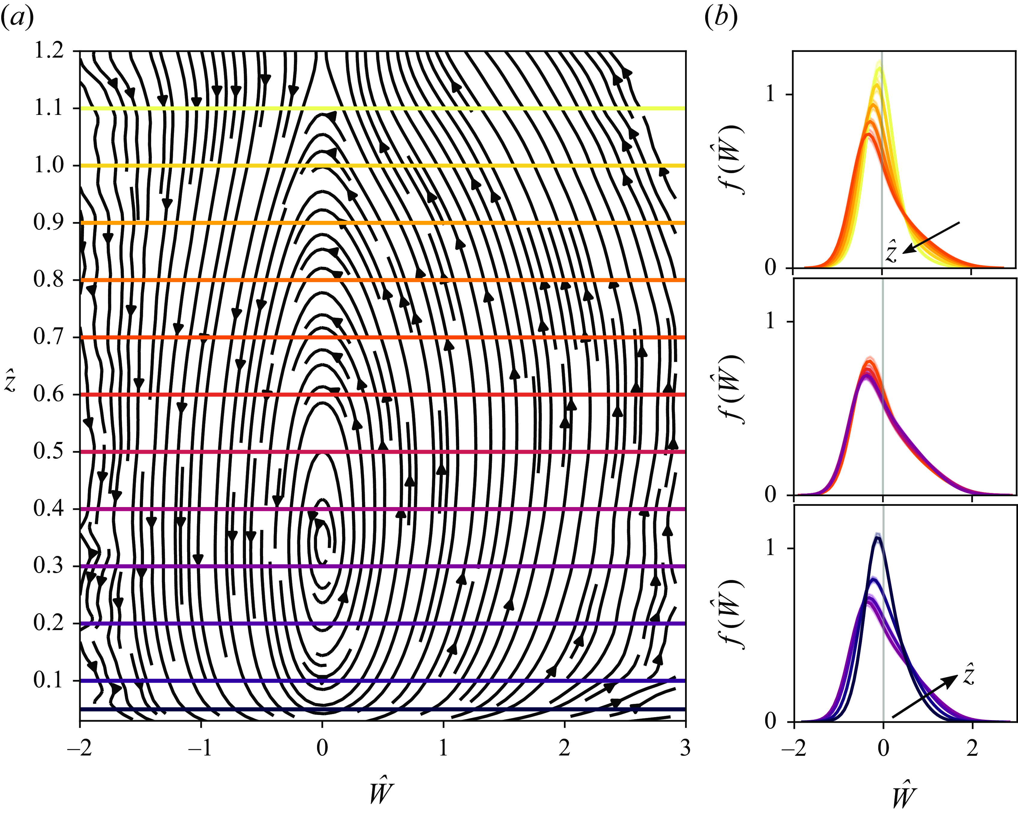
To interpret figure 3, imagine a fluid element with initial coordinates $\hat {z} = 0.2$
and
$\hat {z} = 0.2$
and $\hat {W}=\,1.5$
in the phase space. This fluid element will, on average, follow the vector field that defines the corresponding characteristic line. It rises up according to a path (black arrows in figure 3
a) given by the conditional averages, changing with it its velocity and its height. More generally, considering the PDF and not only a fluid element,
$\hat {W}=\,1.5$
in the phase space. This fluid element will, on average, follow the vector field that defines the corresponding characteristic line. It rises up according to a path (black arrows in figure 3
a) given by the conditional averages, changing with it its velocity and its height. More generally, considering the PDF and not only a fluid element, $f(\hat {W};\hat {z})$
will evolve in height following a path given by the characteristic lines. Such evolution for different heights is shown in the three plots in figure 3(b). The black arrows on the tails of positive
$f(\hat {W};\hat {z})$
will evolve in height following a path given by the characteristic lines. Such evolution for different heights is shown in the three plots in figure 3(b). The black arrows on the tails of positive $\hat {W}$
of the PDFs indicate how the tails of the PDF expand (contract) as the value of
$\hat {W}$
of the PDFs indicate how the tails of the PDF expand (contract) as the value of $\hat {z}$
increases. Hence at any particular height and for positive velocities, a positive value of the balance of the terms means that the tail of the PDF will expand towards larger values of
$\hat {z}$
increases. Hence at any particular height and for positive velocities, a positive value of the balance of the terms means that the tail of the PDF will expand towards larger values of $\hat {W}$
, while negative values of the sum of the terms mean that the tail of
$\hat {W}$
, while negative values of the sum of the terms mean that the tail of $f(\hat {W};\hat {z})$
will contract to smaller values of
$f(\hat {W};\hat {z})$
will contract to smaller values of $\hat {W}$
. Negative velocities have a similar interpretation: positive values of the balance of the terms mean that the tail of the PDF will contract to ’less negative’ values in
$\hat {W}$
. Negative velocities have a similar interpretation: positive values of the balance of the terms mean that the tail of the PDF will contract to ’less negative’ values in $\hat {W}$
, while negative values mean that the tail of the PDF will expand to larger ’more negative’ values of the vertical velocity.
$\hat {W}$
, while negative values mean that the tail of the PDF will expand to larger ’more negative’ values of the vertical velocity.
There are two more aspects to highlight regarding figure 3 and (3.8). First, notice that the concentration of particles following any characteristic at a particular location in the phase space is directly linked to the magnitude of the PDF for vertical velocity at that point in the phase space $f(\hat {W}';\hat {z}')$
. This means that there are more conditional particles following the characteristics at a point
$f(\hat {W}';\hat {z}')$
. This means that there are more conditional particles following the characteristics at a point $(\hat {W}_1,\hat {z}_1)$
than at a point
$(\hat {W}_1,\hat {z}_1)$
than at a point $(\hat {W}_2,\hat {z}_2)$
if
$(\hat {W}_2,\hat {z}_2)$
if $f(\hat {W}_1;\hat {z}_1)\gt f(\hat {W}_2;\hat {z}_2)$
. Second, the characteristics cannot converge to a limit cycle; instead, they must shape closed curves; see Lülff et al. (Reference Lülff, Wilczek, Stevens, Friedrich and Lohse2015), who present a deeper analysis of this argument for an RBC cell.
$f(\hat {W}_1;\hat {z}_1)\gt f(\hat {W}_2;\hat {z}_2)$
. Second, the characteristics cannot converge to a limit cycle; instead, they must shape closed curves; see Lülff et al. (Reference Lülff, Wilczek, Stevens, Friedrich and Lohse2015), who present a deeper analysis of this argument for an RBC cell.
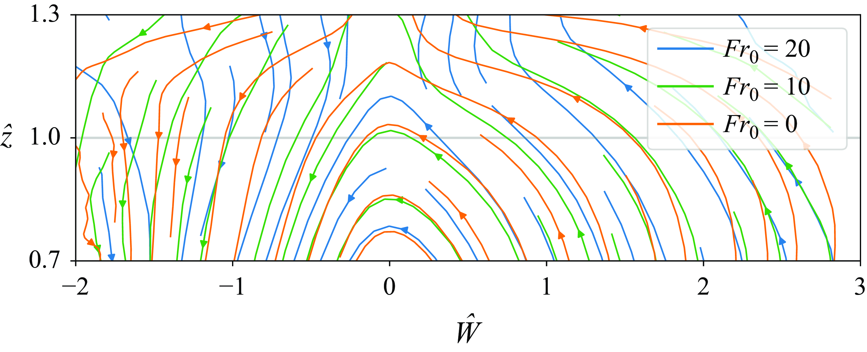
Qualitatively, the characteristics are very similar for the different Froude numbers that we considered. The main difference for the characteristic trajectories between the different Froude numbers occurs in the entrainment zone, shown in figure 4, where the boundary layer starts relaxing into the free atmosphere. The differences are presumably due to the effect of wind shear or the lack of it.
Characteristics of CBLs with ${\textit {Re}}_0 = 42$
, for different Froude numbers. The arrows represent the streamlines defined by the vector field in (3.8). Only the higher altitudes (
${\textit {Re}}_0 = 42$
, for different Froude numbers. The arrows represent the streamlines defined by the vector field in (3.8). Only the higher altitudes ( $\hat {z}=0.7{-}1.3$
) of the CBLs are shown here.
$\hat {z}=0.7{-}1.3$
) of the CBLs are shown here.
To summarise, by examining the PDF equation with appropriate scaling, employing the method of characteristics, and incorporating data from DNS, we gained insights into the average behaviour of CBLs.
3.1.3. Moments of the PDF
As mentioned, higher-order velocity statistics, in particular third and fourth moments of the PDF, provide useful information about the structure of turbulence in CBLs (Lenschow et al. Reference Lenschow, Lothon, Mayor, Sullivan and Canut2012). Skewness is one of the most relevant moments of the PDF of vertical velocity when studying CBLs since it contains information about the updrafts and downdrafts. The CBLs are characterised by a trend of positive skewness that increases with height (Moeng & Rotunno Reference Moeng and Rotunno1990; Wyngaard Reference Wyngaard2010; Berg et al. Reference Berg, Newsom and Turner2017; Fitch Reference Fitch2019), which is due to how turbulence is typically organised in the CBL: strong updrafts, which occupy a small horizontal area, are located between downdraft areas with lower velocities, which occupy a larger horizontal area. The increase of skewness with height means that the updrafts become stronger and narrower.
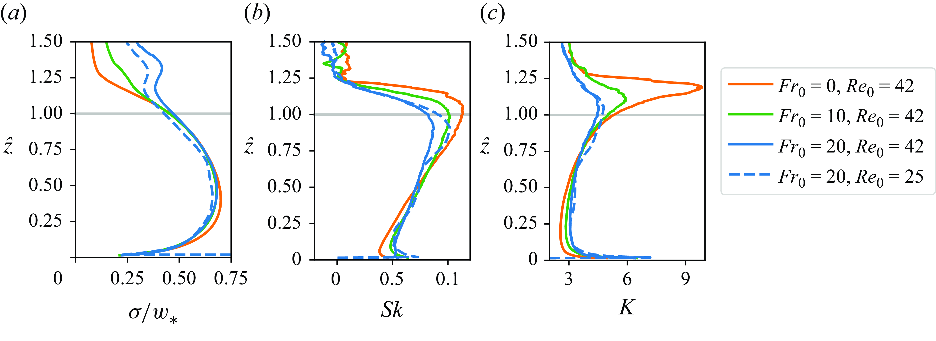
Figure 5 shows the second moment along with the skewness and kurtosis of $f(\hat {W};\hat {z})$
for different atmospheric conditions, each with different conditions of shear, i.e. different values for the horizontal wind in their free atmosphere. The standard deviation exhibits the expected shape of these vertical profiles (from simulations, Schmidt & Schumann Reference Schmidt and Schumann1989; Moeng & Sullivan Reference Moeng and Sullivan1994; Garcia Reference Garcia2014; Mellado et al. Reference Mellado, van Heerwaarden and Garcia2016; Haghshenas & Mellado Reference Haghshenas and Mellado2019; from measurements, Stull Reference Stull1988; Schmidt & Schumann Reference Schmidt and Schumann1989; Wyngaard Reference Wyngaard2010; Berg et al. Reference Berg, Newsom and Turner2017). The observed skewness aligns with the results obtained by others for a midday CBL, as demonstrated in simulations by Moeng & Rotunno (Reference Moeng and Rotunno1990), Lenschow et al. (Reference Lenschow, Lothon, Mayor, Sullivan and Canut2012) and Mellado et al. (Reference Mellado, van Heerwaarden and Garcia2016), as well as in measurements by Lenschow et al. (Reference Lenschow, Lothon, Mayor, Sullivan and Canut2012) and Berg et al. (Reference Berg, Newsom and Turner2017). Additionally, the vertical kurtosis profile depicted in figure 5 indicates that the PDF of vertical velocities near the top of the CBL, at
$f(\hat {W};\hat {z})$
for different atmospheric conditions, each with different conditions of shear, i.e. different values for the horizontal wind in their free atmosphere. The standard deviation exhibits the expected shape of these vertical profiles (from simulations, Schmidt & Schumann Reference Schmidt and Schumann1989; Moeng & Sullivan Reference Moeng and Sullivan1994; Garcia Reference Garcia2014; Mellado et al. Reference Mellado, van Heerwaarden and Garcia2016; Haghshenas & Mellado Reference Haghshenas and Mellado2019; from measurements, Stull Reference Stull1988; Schmidt & Schumann Reference Schmidt and Schumann1989; Wyngaard Reference Wyngaard2010; Berg et al. Reference Berg, Newsom and Turner2017). The observed skewness aligns with the results obtained by others for a midday CBL, as demonstrated in simulations by Moeng & Rotunno (Reference Moeng and Rotunno1990), Lenschow et al. (Reference Lenschow, Lothon, Mayor, Sullivan and Canut2012) and Mellado et al. (Reference Mellado, van Heerwaarden and Garcia2016), as well as in measurements by Lenschow et al. (Reference Lenschow, Lothon, Mayor, Sullivan and Canut2012) and Berg et al. (Reference Berg, Newsom and Turner2017). Additionally, the vertical kurtosis profile depicted in figure 5 indicates that the PDF of vertical velocities near the top of the CBL, at $z_{{enc}}$
, exhibits a higher frequency of outliers compared to lower altitudes. However, the distribution itself tends to be narrower, with an increased probability of small values around the mean, as evidenced by smaller variance values at those heights. This observation aligns with the findings reported in Berg et al. (Reference Berg, Newsom and Turner2017).
$z_{{enc}}$
, exhibits a higher frequency of outliers compared to lower altitudes. However, the distribution itself tends to be narrower, with an increased probability of small values around the mean, as evidenced by smaller variance values at those heights. This observation aligns with the findings reported in Berg et al. (Reference Berg, Newsom and Turner2017).
(a) Standard deviation, (b) skewness and (c) kurtosis of $f(\hat {W})$
. The different colours correspond to the different atmospheric conditions. The horizontal grey line indicates the depth of the CBL,
$f(\hat {W})$
. The different colours correspond to the different atmospheric conditions. The horizontal grey line indicates the depth of the CBL, $z_{{enc}}$
.
$z_{{enc}}$
.
To expand the analysis on the third moment, we obtained an evolution equation in height by multiplying (3.5) with $(\hat {W}-\langle \hat {U}_z \rangle )^2$
and then integrating over the velocity space:
$(\hat {W}-\langle \hat {U}_z \rangle )^2$
and then integrating over the velocity space:
 \begin{equation} \frac {\partial }{\partial \hat {z}} \langle \hat {u}'^3_z \rangle = 2 \langle \hat {u}'_z \hat {b}' \rangle - 2 \Big \langle \hat {u}'_z \frac {\partial }{\partial \hat {z}} \hat {p} '\Big \rangle + 2\, {\textit {Re}}_*^{-1}\, \langle \hat {u}'_z \hat \nabla ^2 \hat {u}'_z \rangle - \frac {1}{3\hat {t}} \langle \hat {u}^{\prime 2} _z \rangle . \end{equation}
Here, we have once more considered that $\langle \hat {U}_z \rangle \approx 0$
. See Appendix C for the detailed derivation as a well as detailed analysis of the equation.
$\langle \hat {U}_z \rangle \approx 0$
. See Appendix C for the detailed derivation as a well as detailed analysis of the equation.
To better understand the impact of the PDF and the conditional means on the vertical evolution of $\langle \hat {u}'^3_z \rangle$
, we analysed the equation leading up to (3.10), i.e. before integrating over
$\langle \hat {u}'^3_z \rangle$
, we analysed the equation leading up to (3.10), i.e. before integrating over $\hat {W}$
. The analysis showed how for the first half of the mixed layer and regardless of the Froude number values, the buoyancy term in the equation, namely the heat flux, is the term with the greatest impact on the evolution of the third moment, whereas for the second half of the mixed layer, the vertical pressure gradient force together with the dissipative term take over (see figure 14). Furthermore, all along the CBL depth, it is the positive velocity fluctuations that have the strongest influence on shaping the third moment’s vertical evolution, hence the positive value for skewness.
$\hat {W}$
. The analysis showed how for the first half of the mixed layer and regardless of the Froude number values, the buoyancy term in the equation, namely the heat flux, is the term with the greatest impact on the evolution of the third moment, whereas for the second half of the mixed layer, the vertical pressure gradient force together with the dissipative term take over (see figure 14). Furthermore, all along the CBL depth, it is the positive velocity fluctuations that have the strongest influence on shaping the third moment’s vertical evolution, hence the positive value for skewness.
We have also analysed the evolution equation for the normal Reynolds stress. This equation includes terms for turbulent transport, heat flux, pressure redistribution and dissipation, and a quasi-steady term that comes from the standardisation of (3.3) with the convective scales; but it has no source term or mean-flow-advection term. From these terms, the dominant source term for the budget of the Reynolds stress in the mixed layer is the heat flux; in this region, the pressure transport dominates as a sink term except near the wall, where dissipation takes over. For the shear-free case, the pressure term dominates also close to the wall. A deeper analysis of the results is presented in Appendix C.
3.2. Buoyancy
In this subsection, we focus on the buoyancy statistics to complement the analysis of the vertical velocity statistics and to better understand the similarities, differences and the relationship between buoyancy and vertical velocity. As in the case of the vertical velocity, we discuss the marginal PDF, the method of characteristics and the moments of the PDF.
3.2.1. The PDF equation
Just as in the case of the vertical velocity PDF, we obtain an evolution equation for the PDF of buoyancy by marginalising (3.2). The resulting evolution equation for $f(\theta ;z,t)$
takes the form
$f(\theta ;z,t)$
takes the form
 \begin{equation} \frac {\partial }{\partial t}f(\theta ;z,t) + \frac {\partial }{\partial z} \left [ \langle U_z \,|\,\theta ;z,t\rangle\, f(\theta ;z,t) \right ] = - \frac {\partial }{\partial \theta } \left [ f(\theta ;z,t)\, \langle \kappa _b\, \nabla ^2 b \, |\, \theta ;z,t \rangle \right ]. \end{equation}
Here, $\theta$
is the sample-space variable that corresponds to the buoyancy. Compared to the closed advective term in (3.3), the advective term on the left-hand side of this equation contains the unclosed mean velocity conditioned on
$\theta$
is the sample-space variable that corresponds to the buoyancy. Compared to the closed advective term in (3.3), the advective term on the left-hand side of this equation contains the unclosed mean velocity conditioned on $\theta$
, which we evaluate from our numerical data below.
$\theta$
, which we evaluate from our numerical data below.
When evaluating these numerical data, we have once more replaced the ensemble average used for the theoretical derivation by a horizontal and time average.
As we demonstrate in Appendix A, the PDF of buoyancy is approximately self-similar in time and can be collapsed by the rescaling
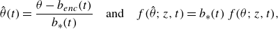 \begin{equation} \hat {\theta }(t) = \dfrac {\theta - b_{{enc}}(t)}{b_*(t)} \quad\text {and}\quad f(\hat {\theta };z, t) = b_*(t)\, f(\theta ;z,t), \end{equation}
with $b_{{enc}}(t) = N_0^2\, z_{{enc}}(t)$
. Following this non-dimensionalisation, the PDF becomes quasi-stationary. As a result, we obtain the non-dimensional form of (3.11):
$b_{{enc}}(t) = N_0^2\, z_{{enc}}(t)$
. Following this non-dimensionalisation, the PDF becomes quasi-stationary. As a result, we obtain the non-dimensional form of (3.11):
 \begin{align} \dfrac {\partial }{\partial \hat {z}} \langle \hat {U}_z \, |\, \hat {\theta };\hat {z} \rangle\, f ( \hat {\theta };\hat {z}) \approx - \dfrac {\partial }{\partial \hat {\theta }} \left [ f(\hat {\theta };\hat {z}) \left ({\textit {Re}}_*^{-1}\, Pr^{-1}\, \langle \hat \nabla ^2 \hat {b} \, |\,\hat {\theta };\hat {z} \rangle + \frac {1}{6 \hat {t}} \hat {\theta } -\dfrac {1}{2\hat {t}} \dfrac {b_{{enc}}}{b_*} \right )\right ],\nonumber\\[3pt] \end{align}
where $Pr = \nu /\kappa _b$
is the molecular Prandtl number. The two extra terms, or quasi-steady terms, on the right-hand side originate from the time dependence of
$Pr = \nu /\kappa _b$
is the molecular Prandtl number. The two extra terms, or quasi-steady terms, on the right-hand side originate from the time dependence of $b_{{enc}}$
and
$b_{{enc}}$
and $b_*$
used in the non-dimensionalisation (3.12) of (3.11).
$b_*$
used in the non-dimensionalisation (3.12) of (3.11).


Figure 6 shows the different terms in (3.13) for the different heights. Figure 6(a) shows the vertical velocity conditioned on $\hat {\theta }$
, which represents the average velocity of fluid parcels with a buoyancy value of
$\hat {\theta }$
, which represents the average velocity of fluid parcels with a buoyancy value of $\hat {\theta }$
. The behaviour of
$\hat {\theta }$
. The behaviour of $\langle \hat {U}_z \,|\,\hat {\theta };\hat {z}\rangle$
for heights close to
$\langle \hat {U}_z \,|\,\hat {\theta };\hat {z}\rangle$
for heights close to $z_{{enc}}$
is particularly interesting. For these heights,
$z_{{enc}}$
is particularly interesting. For these heights, $\hat {z} = 0.95$
,
$\hat {z} = 0.95$
, $1.0$
and
$1.0$
and $1.05$
in the figure, positively buoyant fluid parcels have negative mean velocities, sinking into the CBL instead of rising up. This counterintuitive behaviour represents the entrainment of the free atmosphere into the CBL, and it is consistent with a similar observation in figure 2, which shows the buoyancy conditioned on the vertical velocity.
$1.05$
in the figure, positively buoyant fluid parcels have negative mean velocities, sinking into the CBL instead of rising up. This counterintuitive behaviour represents the entrainment of the free atmosphere into the CBL, and it is consistent with a similar observation in figure 2, which shows the buoyancy conditioned on the vertical velocity.
Figure 6(b) shows the balance of the different terms on the right-hand side of (3.13). The individual terms are not shown since the term proportional to $\hat {\theta }$
and the one proportional to
$\hat {\theta }$
and the one proportional to $b_{{enc}}/b_*$
are an order of magnitude smaller than
$b_{{enc}}/b_*$
are an order of magnitude smaller than $Re_*^{-1}\, Pr^{-1}\, \langle \hat \nabla ^2 \hat {b} \,|\,\hat {\theta };\hat {z} \rangle$
. For the viscous term of the vertical velocity in (3.5), we have seen that it has an overall damping effect towards
$Re_*^{-1}\, Pr^{-1}\, \langle \hat \nabla ^2 \hat {b} \,|\,\hat {\theta };\hat {z} \rangle$
. For the viscous term of the vertical velocity in (3.5), we have seen that it has an overall damping effect towards $\hat {W} \approx \langle \hat {U}_z \rangle \approx 0$
(see figure 2). Contrary to that, the diffusive term for the buoyancy in (3.13) is not necessarily damping. For example, close to the surface, for
$\hat {W} \approx \langle \hat {U}_z \rangle \approx 0$
(see figure 2). Contrary to that, the diffusive term for the buoyancy in (3.13) is not necessarily damping. For example, close to the surface, for $\hat {z}= 0.05$
and
$\hat {z}= 0.05$
and $0.2$
in figure 6, this term is positive and has a maximum in its amplitude at
$0.2$
in figure 6, this term is positive and has a maximum in its amplitude at $\hat {\theta } \approx \langle \hat {b} \rangle$
. This means that at these heights, neutrally buoyant fluid parcels are being heated up. This is as a result of the heating imposed at the surface by the buoyancy flux
$\hat {\theta } \approx \langle \hat {b} \rangle$
. This means that at these heights, neutrally buoyant fluid parcels are being heated up. This is as a result of the heating imposed at the surface by the buoyancy flux $B_0$
. This observation is similar to previous observations in RBC (see figure 4(b) in Lülff et al. Reference Lülff, Wilczek and Friedrich2011). For regions close to the bottom boundary, the diffusion terms for RBC and CBL behave similarly for positive values of buoyancy. For negative values near the surface, however, we observe differences between RBC and the CBL: the diffusion term for the RBC cell is always positive and with amplitudes comparable to those of the positive values of buoyancy, whereas that for the CBL has close to zero values for
$B_0$
. This observation is similar to previous observations in RBC (see figure 4(b) in Lülff et al. Reference Lülff, Wilczek and Friedrich2011). For regions close to the bottom boundary, the diffusion terms for RBC and CBL behave similarly for positive values of buoyancy. For negative values near the surface, however, we observe differences between RBC and the CBL: the diffusion term for the RBC cell is always positive and with amplitudes comparable to those of the positive values of buoyancy, whereas that for the CBL has close to zero values for $\hat {z}= 0.05$
and even negative small amplitudes when the height increases. These differences are due to the upper region of the system. The RBC cell exhibits the effects of the cooling of the upper plate, whereas the CBL shows the effects of the entrainment of buoyant air from the free atmosphere.
$\hat {z}= 0.05$
and even negative small amplitudes when the height increases. These differences are due to the upper region of the system. The RBC cell exhibits the effects of the cooling of the upper plate, whereas the CBL shows the effects of the entrainment of buoyant air from the free atmosphere.
3.2.2. Method of characteristics
As occurred with the vertical velocity component, the evolution equation for the PDF of buoyancy, (3.13), is a first-order PDE that can be analysed using the method of characteristics to help us to understand the average behaviour of fluid parcels in the buoyancy space. For the case of buoyancy, the phase space is given by $(\hat {\theta },\hat {z})$
, and the characteristic trajectories are
$(\hat {\theta },\hat {z})$
, and the characteristic trajectories are
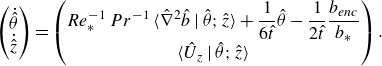 \begin{equation} \begin{pmatrix} \dot {\hat {\theta }}\\ \dot {\hat {z}} \end{pmatrix} = \begin{pmatrix} Re_*^{-1}\, Pr^{-1}\, \langle \hat \nabla ^2 \hat {b} \,|\,\hat {\theta };\hat {z} \rangle + \dfrac {1}{6 \hat {t}} \hat {\theta } -\dfrac {1}{2\hat {t}} \dfrac {b_{{enc}}}{b_*}\\[4pt] \langle \hat {U}_z \, |\,\hat {\theta };\hat {z}\rangle \end{pmatrix}. \end{equation}
Once more, the dot notation refers to a derivative with respect to a parameter $s$
. The buoyancy PDF along a characteristic parametrised by
$s$
. The buoyancy PDF along a characteristic parametrised by $s$
starting from
$s$
starting from $\hat {\theta }(s_0)$
and
$\hat {\theta }(s_0)$
and $\hat {z}(s_0)$
evolves according to
$\hat {z}(s_0)$
evolves according to
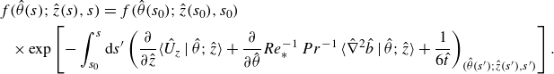 \begin{align} f & (\hat {\theta }(s); \hat {z}(s), s) = f(\hat {\theta }(s_0); \hat {z}(s_0), s_0)\nonumber \\ & {}\times \exp \left [ -\int ^{s}_{s_0} {\rm d}s'\left ( \frac {\partial }{\partial \hat { z}} \langle \hat {U}_z \, |\,\hat {\theta };\hat {z}\rangle + \frac {\partial }{\partial \hat {\theta }} Re_*^{-1}\, Pr^{-1}\, \langle \hat \nabla ^2 \hat {b} \, |\,\hat {\theta }; \hat {z}\rangle + \frac {1}{6 \hat {t}} \right )_{(\hat {\theta }(s'); \hat {z}(s'), s')} \right ].\nonumber\\[4pt] \end{align}
Figure 7(a) shows the characteristic curves, i.e. the streamlines of the vector field given by the right-hand side of (3.14) for a CBL with ${\textit {Re}}_0 = 42$
and
${\textit {Re}}_0 = 42$
and $Fr_0=20$
.
$Fr_0=20$
.
For heights in the mixed layer, between the bottom boundary and the entrainment zone, the characteristic curves indicate a circular motion. This means that on average, a conditional particle with a buoyancy larger than the mean will rise while gradually losing buoyancy. When it reaches the entrainment zone, it loses buoyancy while staying near the entrainment zone, then sinks to the bottom once its buoyancy is smaller than the mean. As can be seen from the slopes of the characteristic curves, the buoyancy changes only little while the conditional particle sinks to the bottom. As shown in figure 7(b), the PDFs change only little within the well-mixed layer, as expected from the non-dimensionalisation with the mixed-layer scaling, while the PDFs vary more strongly closer to the bottom wall, where surface scaling applies instead of mixed-layer scaling.
In the entrainment zone, a secondary circulation motion can be seen, which can be interpreted as the average entrainment of conditional particles from upper atmospheric layers. Buoyant conditional particles from the free atmosphere are entrained and rapidly lose buoyancy towards the buoyancy values that are observed in the mixed layer. The corresponding PDFs also vary appreciably within this range of heights.
All cases of $Fr_0$
that we analysed present the same behaviour. The difference between the Froude number cases occurs in the entrainment zone, where for the cases
$Fr_0$
that we analysed present the same behaviour. The difference between the Froude number cases occurs in the entrainment zone, where for the cases $Fr_0 = 10$
and
$Fr_0 = 10$
and $Fr_0 = 0$
, the PDF starts to evolve into a bimodal one; see figure 7.
$Fr_0 = 0$
, the PDF starts to evolve into a bimodal one; see figure 7.
(a) Characteristics defined by the vector field in (3.14) for a CBL with ${\textit {Re}}_0 = 42$
and
${\textit {Re}}_0 = 42$
and $Fr_0=20$
. The vertical profile in blue is the mean value of the standardised buoyancy. (b) Buoyancy PDFs as functions of
$Fr_0=20$
. The vertical profile in blue is the mean value of the standardised buoyancy. (b) Buoyancy PDFs as functions of $\hat {\theta }-\langle \hat {b} \rangle$
. The different colours represent the different altitudes indicated with the horizontal coloured lines in (a). At height
$\hat {\theta }-\langle \hat {b} \rangle$
. The different colours represent the different altitudes indicated with the horizontal coloured lines in (a). At height $\hat {z} = 1.05 z_{{enc}}$
, the PDFs for
$\hat {z} = 1.05 z_{{enc}}$
, the PDFs for $Fr_0=10$
and
$Fr_0=10$
and $0$
are also shown.
$0$
are also shown.
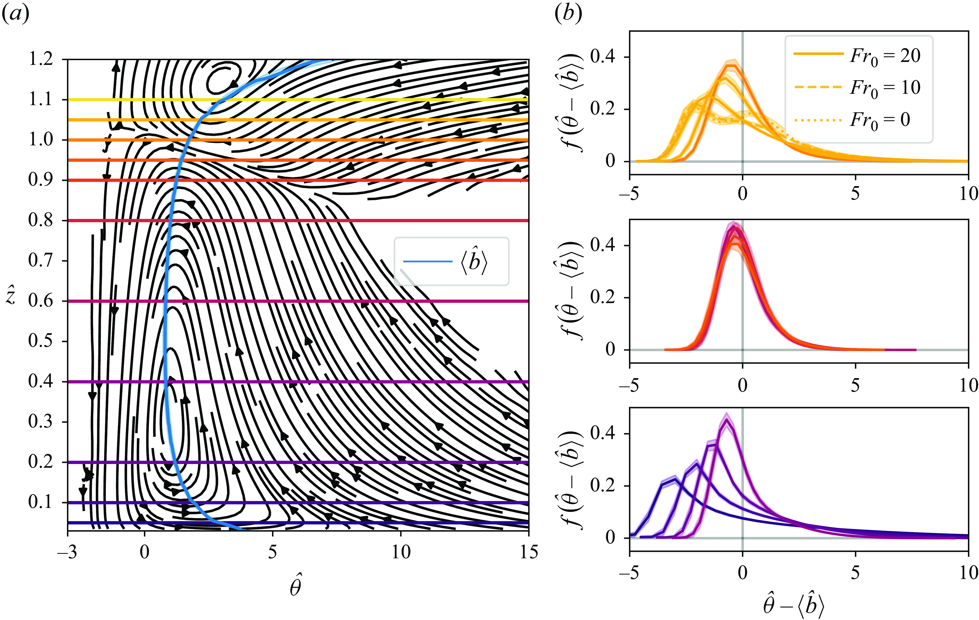
(a) Mean, (b) standard deviation (compare to figure 5 of Schmidt & Schumann Reference Schmidt and Schumann1989), (c) skewness (compare to figure 8 of Mellado et al. Reference Mellado, Puche and van Heerwaarden2017), and(d) kurtosis. The different colours correspond to the different atmospheric conditions. The horizontal grey line indicates the depth of the mixed layer, $z_{{enc}}$
.
$z_{{enc}}$
.
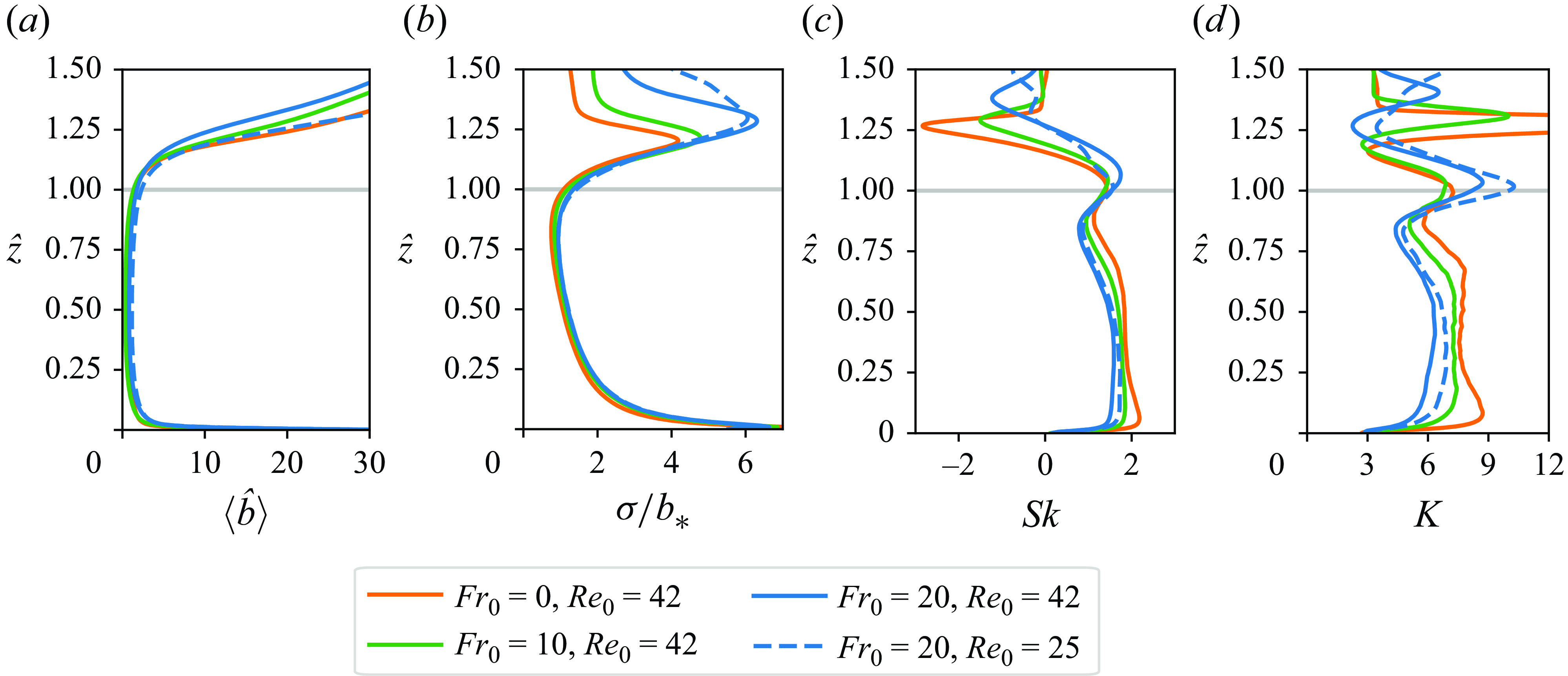
3.2.3. Moments of the PDF
An insight into the spatial structure of convection can be obtained by analysing the vertical structure of the moments of the PDF. Figure 8 shows the vertical profiles of the second moment, the skewness and the kurtosis of $f(\hat {\theta };\hat {z})$
for different CBL conditions, as well as the mean profile for reference.
$f(\hat {\theta };\hat {z})$
for different CBL conditions, as well as the mean profile for reference.
The standard deviation is shown to be independent of the atmospheric conditions within the range considered in this study. Furthermore, an equation for the second moment can be obtained from (3.13):
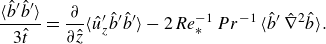 \begin{equation} \frac { \langle \hat {b}' \hat {b}' \rangle }{3 \hat {t}} = \frac {\partial }{\partial \hat {z}} \langle \hat {u}'_z \hat {b}' \hat {b}' \rangle - 2\, {\textit {Re}}_*^{-1}\,Pr^{-1}\, \langle \hat {b}'\, \hat \nabla ^2 \hat {b} \rangle . \end{equation}
This equation might seem to contradict our assumption of ${\partial }\langle \hat {b}'\hat {b}'\rangle /{\partial \hat {t}}\approx 0$
. Nonetheless, in the well-mixed layer, the region characterised by the convective scales, the term
${\partial }\langle \hat {b}'\hat {b}'\rangle /{\partial \hat {t}}\approx 0$
. Nonetheless, in the well-mixed layer, the region characterised by the convective scales, the term ${ \langle \hat {b}' \hat {b}' \rangle }/{3 \hat {t}}$
is negligible, and the dominant balance in the equation occurs between the turbulent transport term and the dissipation term on the right-hand side. In the entrainment zone and near-surface region, the term
${ \langle \hat {b}' \hat {b}' \rangle }/{3 \hat {t}}$
is negligible, and the dominant balance in the equation occurs between the turbulent transport term and the dissipation term on the right-hand side. In the entrainment zone and near-surface region, the term ${ \langle \hat {b}' \hat {b}' \rangle }/{3 \hat {t}}$
is not negligible; nonetheless, these regions are characterised by different scalings, as discussed e.g. by Haghshenas & Mellado (Reference Haghshenas and Mellado2019) and Fodor et al. (Reference Fodor, Mellado and Haghshenas2022) in the first case, and by Fodor (Reference Fodor2020) in the second case. Therefore, although the term
${ \langle \hat {b}' \hat {b}' \rangle }/{3 \hat {t}}$
is not negligible; nonetheless, these regions are characterised by different scalings, as discussed e.g. by Haghshenas & Mellado (Reference Haghshenas and Mellado2019) and Fodor et al. (Reference Fodor, Mellado and Haghshenas2022) in the first case, and by Fodor (Reference Fodor2020) in the second case. Therefore, although the term ${ \langle \hat {b}' \hat {b}' \rangle }/{3 \hat {t}}$
shows the effects of the time evolution of the convective scales, it does not contradict our stationarity assumption in the mixed layer.
${ \langle \hat {b}' \hat {b}' \rangle }/{3 \hat {t}}$
shows the effects of the time evolution of the convective scales, it does not contradict our stationarity assumption in the mixed layer.
Contrary to the standard deviation, skewness and kurtosis do vary depending on the atmospheric conditions. Shear-free CBLs have a larger value of skewness and kurtosis than sheared CBLs everywhere in the CBL except in the entrainment zone, the region between $\hat {z}=1.0$
and
$\hat {z}=1.0$
and $\hat {z}=1.25$
. There, skewness and kurtosis increase for the cases where shear is present. This indicates the different roles of wind shear in the mixed layer and in the entrainment zone. In the mixed layer, the mean wind shear increases mixing, which reduces the skewness. In the entrainment zone, wind shear increases the entrainment of buoyant parcels from the free atmosphere, with properties that are very different from the mixed-layer properties, and this leads to greater values of positive outliers.
$\hat {z}=1.25$
. There, skewness and kurtosis increase for the cases where shear is present. This indicates the different roles of wind shear in the mixed layer and in the entrainment zone. In the mixed layer, the mean wind shear increases mixing, which reduces the skewness. In the entrainment zone, wind shear increases the entrainment of buoyant parcels from the free atmosphere, with properties that are very different from the mixed-layer properties, and this leads to greater values of positive outliers.
Regarding the sensitivity of the profiles to the different values of the Reynolds number, it is already relatively small for the Reynolds numbers that we start to reach in numerical simulations, in particular in the mixed layer, as shown in figure 8. There, although an effect of the Reynolds number is observed, this effect is smaller than the effect of changing the Froude number. Low-Reynolds-number effects appear stronger in the entrainment zone, relative to the effect of changing $Fr_0$
, consistent with previous analysis (Mellado et al. Reference Mellado, Puche and van Heerwaarden2017).
$Fr_0$
, consistent with previous analysis (Mellado et al. Reference Mellado, Puche and van Heerwaarden2017).
3.3. Area fractions
A comprehensive analysis of how vertical velocity is distributed between vertical drafts in CBLs to correctly represent vertical transport, and its link to different atmospheric processes and models, remains a challenge (Suselj et al. Reference Suselj, Kurowski and Teixeira2019; Fitch Reference Fitch2019; Witte et al. Reference Witte, Herrington, Teixeira, Kurowski, Chinita, Storer, Suselj, Matheou and Bacmeister2022). As a contribution to this line of research, we also investigated turbulent vertical velocity and buoyancy fields in a CBL focusing on the updrafts and downdrafts, and buoyant and non-buoyant contributions of convective structures. To do so, we analyse area fractions of the different contributions to the marginal PDFs of vertical velocity and buoyancy.
Area fractions of the updrafts from the marginal PDF of (a) vertical velocity, and (b) the buoyant regions from the marginal PDF of buoyancy of the different CBLs that we analyse. The schematics on the top illustrate the definition of the different area fractions, red colour highlighting the area fraction plotted below. They show the sample space of the joint PDF of vertical velocity and buoyancy, $(\hat {W},\hat {\theta })$
at any particular height, and the coloured regions correspond to the different limits of the integrals in (3.17) and (3.18).
$(\hat {W},\hat {\theta })$
at any particular height, and the coloured regions correspond to the different limits of the integrals in (3.17) and (3.18).
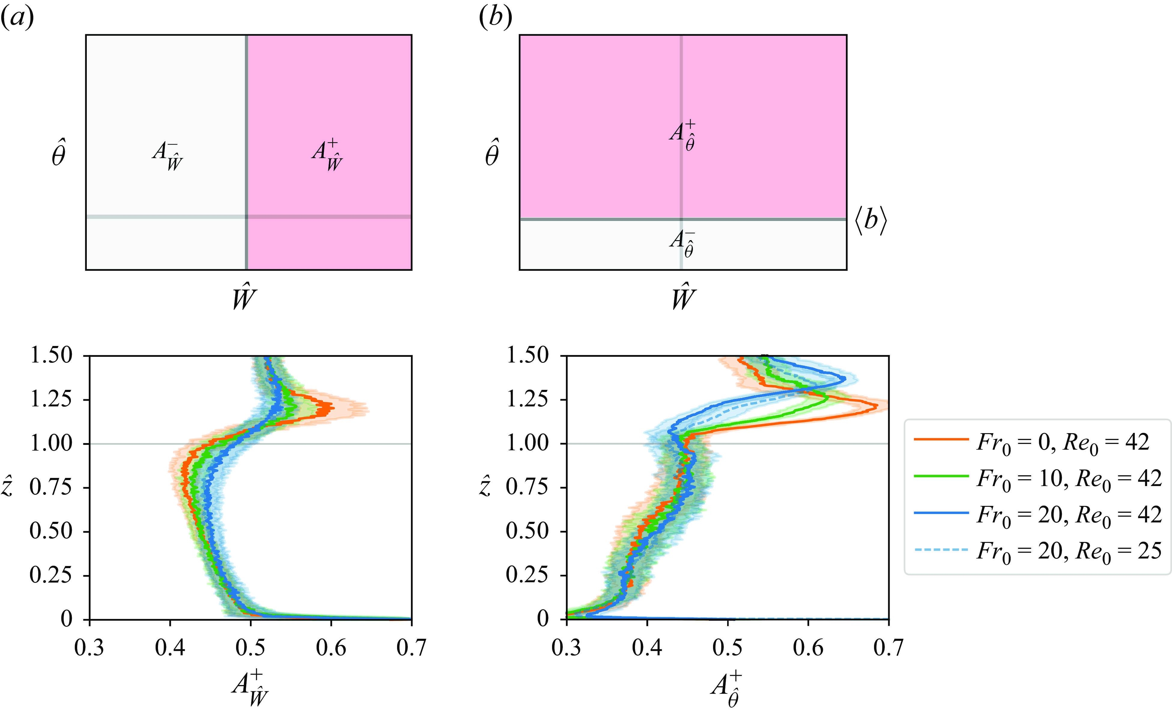
The area fraction of the buoyant contribution to the joint PDF of vertical velocity and buoyancy is defined as (see figure 9)
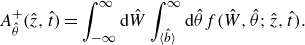 \begin{equation} A^+_{\hat {\theta }}(\hat {z},\hat {t}) =\int _{-\infty }^\infty {\rm d}\hat {W} \int _{\langle \hat {b} \rangle } ^\infty {\rm d}\hat {\theta } f(\hat {W}, \hat {\theta };\hat {z},\hat {t}). \end{equation}
By the law of total probability, the area fraction of the non-buoyant contribution is $A_{\hat {\theta }}^-(\hat {z},\hat {t} ) =1- A_{\hat {\theta }}^+(\hat {z},\hat {t} )$
. On the other hand, the area fraction of the updraft contribution to the PDF is
$A_{\hat {\theta }}^-(\hat {z},\hat {t} ) =1- A_{\hat {\theta }}^+(\hat {z},\hat {t} )$
. On the other hand, the area fraction of the updraft contribution to the PDF is
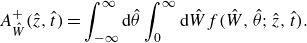 \begin{equation} A^+_{\hat {W}}(\hat {z},\hat {t}) =\int _{-\infty }^\infty {\rm d}\hat {\theta } \int _{0} ^\infty {\rm d}\hat {W} f(\hat {W}, \hat {\theta };\hat {z},\hat {t}). \end{equation}
For this definition we consider that $\langle \hat {U}_z\rangle \approx 0$
, thus the limit of the integral over the velocity space. Analogously,
$\langle \hat {U}_z\rangle \approx 0$
, thus the limit of the integral over the velocity space. Analogously, $A_{\hat {W}}^-(\hat {z},\hat {t} ) =1- A_{\hat {W}}^+(\hat {z},\hat {t} )$
.
$A_{\hat {W}}^-(\hat {z},\hat {t} ) =1- A_{\hat {W}}^+(\hat {z},\hat {t} )$
.
From this approach, we observe that the boundary layer contains non-buoyant parcels of fluid with positive vertical velocities rising into the CBL, and vice versa. Otherwise, if all buoyant parcels of fluid had positive vertical velocities, and all non-buoyant parcels of fluid had negative vertical velocities, then $A^+_{\hat {W}}(\hat {z},\hat {t})$
and
$A^+_{\hat {W}}(\hat {z},\hat {t})$
and $A^+_{\hat {\theta }}(\hat {z},\hat {t})$
, shown on figure 9, would have similar profiles.
$A^+_{\hat {\theta }}(\hat {z},\hat {t})$
, shown on figure 9, would have similar profiles.
The area fraction $A_{\hat {W}}^+(\hat {z},\hat {t} )$
is linked to the skewness of the PDF of vertical velocity, and consequently, the turbulent vertical structure of CBLs. As mentioned above, in boundary layers driven by buoyancy, strong updrafts that occupy small horizontal areas are between downdrafts with smaller velocities occupying larger horizontal areas, and updrafts become narrower with height. The bottom plot in figure 9(a) is in agreement with such a statement when considering the area below the entrainment zone. Nonetheless, in the entrainment zone and above, updrafts become wider before losing area once more as they penetrate into the free atmosphere, which is stably stratified. Regarding the buoyancy, the bottom plot in figure 9(b) gives some insight into the effects of shear in the entrainment zone. For shear-free cases, positively buoyant regions penetrate less into the free atmosphere but rapidly occupy a larger area than in sheared cases. The reason is that wind shear increases mixing locally in the entrainment zone, increasing the entrainment-zone thickness and reducing the horizontal extension of buoyant regions. Above the entrainment zone, turbulence decays and buoyancy fluctuations are caused by the gravity waves in the stably stratified free atmosphere (Carruthers & Hunt Reference Carruthers and Hunt1986), the regions of positive and negative buoyancy occupying half of the total area, and both quantities
$A_{\hat {W}}^+(\hat {z},\hat {t} )$
is linked to the skewness of the PDF of vertical velocity, and consequently, the turbulent vertical structure of CBLs. As mentioned above, in boundary layers driven by buoyancy, strong updrafts that occupy small horizontal areas are between downdrafts with smaller velocities occupying larger horizontal areas, and updrafts become narrower with height. The bottom plot in figure 9(a) is in agreement with such a statement when considering the area below the entrainment zone. Nonetheless, in the entrainment zone and above, updrafts become wider before losing area once more as they penetrate into the free atmosphere, which is stably stratified. Regarding the buoyancy, the bottom plot in figure 9(b) gives some insight into the effects of shear in the entrainment zone. For shear-free cases, positively buoyant regions penetrate less into the free atmosphere but rapidly occupy a larger area than in sheared cases. The reason is that wind shear increases mixing locally in the entrainment zone, increasing the entrainment-zone thickness and reducing the horizontal extension of buoyant regions. Above the entrainment zone, turbulence decays and buoyancy fluctuations are caused by the gravity waves in the stably stratified free atmosphere (Carruthers & Hunt Reference Carruthers and Hunt1986), the regions of positive and negative buoyancy occupying half of the total area, and both quantities $A_{\hat {W}}^+$
and
$A_{\hat {W}}^+$
and $A_{\hat {\theta }}^+$
being approximately 0.5.
$A_{\hat {\theta }}^+$
being approximately 0.5.
Beyond studying area fractions, we also investigate their flux $ A_{\hat {W}}^\pm \langle \hat {U}_z \rangle _\pm$
. We relate this flux of area fraction to the concept of mass flux between updrafts and downdrafts. Historically, the mass flux concept in CBLs originated from the cloud modelling community in the late 1960s and early 1970s. Later, attempts to model turbulent transport in dry CBLs used, as here, a decomposition in updrafts and downdrafts, particularly in two-stream models (Chatfield & Brost Reference Chatfield and Brost1987; Siebesma et al. Reference Siebesma, Soares and Teixeira2007; Gentine et al. Reference Gentine, Betts, Lintner, Findell, Van Heerwaarden, Tzella and d’Andrea2013; Suselj et al. Reference Suselj, Kurowski and Teixeira2019; Witte et al. Reference Witte, Herrington, Teixeira, Kurowski, Chinita, Storer, Suselj, Matheou and Bacmeister2022). These models parametrise vertical turbulent transfer in CBLs by assuming horizontal homogeneity, and consider all CBL air to belong to either an upward-moving stream or a downward-moving one.
$ A_{\hat {W}}^\pm \langle \hat {U}_z \rangle _\pm$
. We relate this flux of area fraction to the concept of mass flux between updrafts and downdrafts. Historically, the mass flux concept in CBLs originated from the cloud modelling community in the late 1960s and early 1970s. Later, attempts to model turbulent transport in dry CBLs used, as here, a decomposition in updrafts and downdrafts, particularly in two-stream models (Chatfield & Brost Reference Chatfield and Brost1987; Siebesma et al. Reference Siebesma, Soares and Teixeira2007; Gentine et al. Reference Gentine, Betts, Lintner, Findell, Van Heerwaarden, Tzella and d’Andrea2013; Suselj et al. Reference Suselj, Kurowski and Teixeira2019; Witte et al. Reference Witte, Herrington, Teixeira, Kurowski, Chinita, Storer, Suselj, Matheou and Bacmeister2022). These models parametrise vertical turbulent transfer in CBLs by assuming horizontal homogeneity, and consider all CBL air to belong to either an upward-moving stream or a downward-moving one.
Following our PDF approach, one can also analyse the mentioned flux of area fraction as a simple consequence of the fundamental theorem of calculus by integrating (3.5) from zero to infinity in the velocity space:
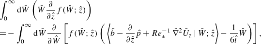 \begin{align} &\int _0^\infty {\rm d}\hat {W} \left (\hat {W} \frac {\partial }{\partial \hat {z}} f(\hat {W};\hat {z})\right ) \nonumber\\ &=- \int _0^\infty {\rm d}\hat {W} \frac {\partial }{\partial \hat {W}} \left [ f(\hat {W};\hat {z}) \left ( \,\left \langle \hat {b} - \frac {\partial }{\partial \hat {z}} \hat {p} + Re_*^{-1}\, \hat \nabla ^2 \hat {U}_z \,\Big |\, \hat {W};\hat {z}\right \rangle - \frac {1}{6\hat {t}} \hat {W} \right ) \right ], \end{align}
then
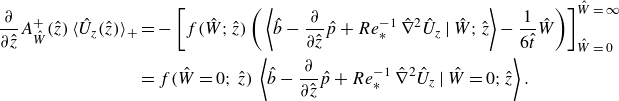 \begin{align} \frac {\partial }{\partial \hat {z}} A_{\hat {W}}^+ (\hat {z})\, \langle \hat {U}_z(\hat {z}) \rangle _+ &= - \left [ f(\hat {W};\hat {z}) \left ( \,\left \langle \hat {b} - \frac {\partial }{\partial \hat {z}} \hat {p} + Re_*^{-1}\, \hat \nabla ^2 \hat {U}_z \,\Big |\, \hat {W};\hat {z}\right \rangle - \frac {1}{6\hat {t}} \hat {W} \right ) \right ] _{\hat {W}\,=\,0}^{\hat {W}\,=\,\infty } \nonumber\\ &= f(\hat {W}=0;\,\hat {z})\,\left \langle \hat {b} - \frac {\partial }{\partial \hat {z}} \hat {p} + Re_*^{-1}\, \hat \nabla ^2 \hat {U}_z \,\Big |\, \hat {W} = 0;\hat {z}\right \rangle . \end{align}
Here, $ \langle \hat {U}_z (\hat {z}) \rangle _\pm$
is the mean of the vertical velocity inside the updrafts (downdrafts):
$ \langle \hat {U}_z (\hat {z}) \rangle _\pm$
is the mean of the vertical velocity inside the updrafts (downdrafts):
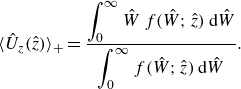 \begin{equation} \langle \hat {U}_z (\hat {z})\rangle _+ = \frac {\displaystyle\int _0^{\infty } \hat {W}\, f(\hat {W};\hat {z})\, {\rm d}\hat {W}}{\displaystyle\int _0^{\infty } f(\hat {W};\hat {z})\, {\rm d}\hat {W}}. \end{equation}
A similar equation for the downdrafts can be obtained by integrating (3.5) from minus infinity to zero:
 \begin{equation} \frac {\partial }{\partial \hat {z}} A_{\hat {W}}^-(\hat {z})\, \langle \hat {U}_z(\hat {z}) \rangle _- = - f(\hat {W}=0;\hat {z})\,\left \langle \hat {b} - \frac {\partial }{\partial \hat {z}} \hat {p} + Re_*^{-1}\, \hat \nabla ^2 \hat {U}_z \,\Big |\, \hat {W} = 0;\hat {z}\right \rangle . \end{equation}
Adding (3.20) and (3.22), the right-hand sides cancel each other, which is consistent with our consideration of zero vertical mean.
Furthermore, any positive change (gain) in height for the flux of area fraction of updrafts ( $ A_{\hat {W}}^+ \langle \hat {U}_z \rangle _+$
) represents a negative change (loss) for the flux of area fraction of downdrafts, and vice versa:
$ A_{\hat {W}}^+ \langle \hat {U}_z \rangle _+$
) represents a negative change (loss) for the flux of area fraction of downdrafts, and vice versa:
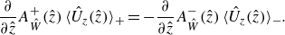 \begin{equation} \frac {\partial }{\partial \hat {z}} A_{\hat {W}}^+ (\hat {z})\, \langle \hat {U}_z(\hat {z}) \rangle _+ = - \frac {\partial }{\partial \hat {z}} A_{\hat {W}}^- (\hat {z})\, \langle \hat {U}_z(\hat {z}) \rangle _-. \end{equation}
The right-hand sides of (3.20) and (3.22) can be interpreted as the mixing term studied by Schumann & Moeng (Reference Schumann and Moeng1991). In general, these equations describe the mass flux between updrafts and downdrafts without attempting to parametrise it, but allowing us to characterise its dynamical nature.
(a) Right-hand side of (3.20) for different atmospheric conditions. (b) Deviations from the hydrostatic balance. The shaded regions indicate the region of the CBL where $\langle \hat {b} \,|\, \hat {W}=0 \rangle \gt \langle {\partial \hat {p}}/{\partial \hat {z}} \,|\, \hat {W}=0 \rangle$
. All profiles represent CBLs with
$\langle \hat {b} \,|\, \hat {W}=0 \rangle \gt \langle {\partial \hat {p}}/{\partial \hat {z}} \,|\, \hat {W}=0 \rangle$
. All profiles represent CBLs with $Re_0 = 42$
.
$Re_0 = 42$
.
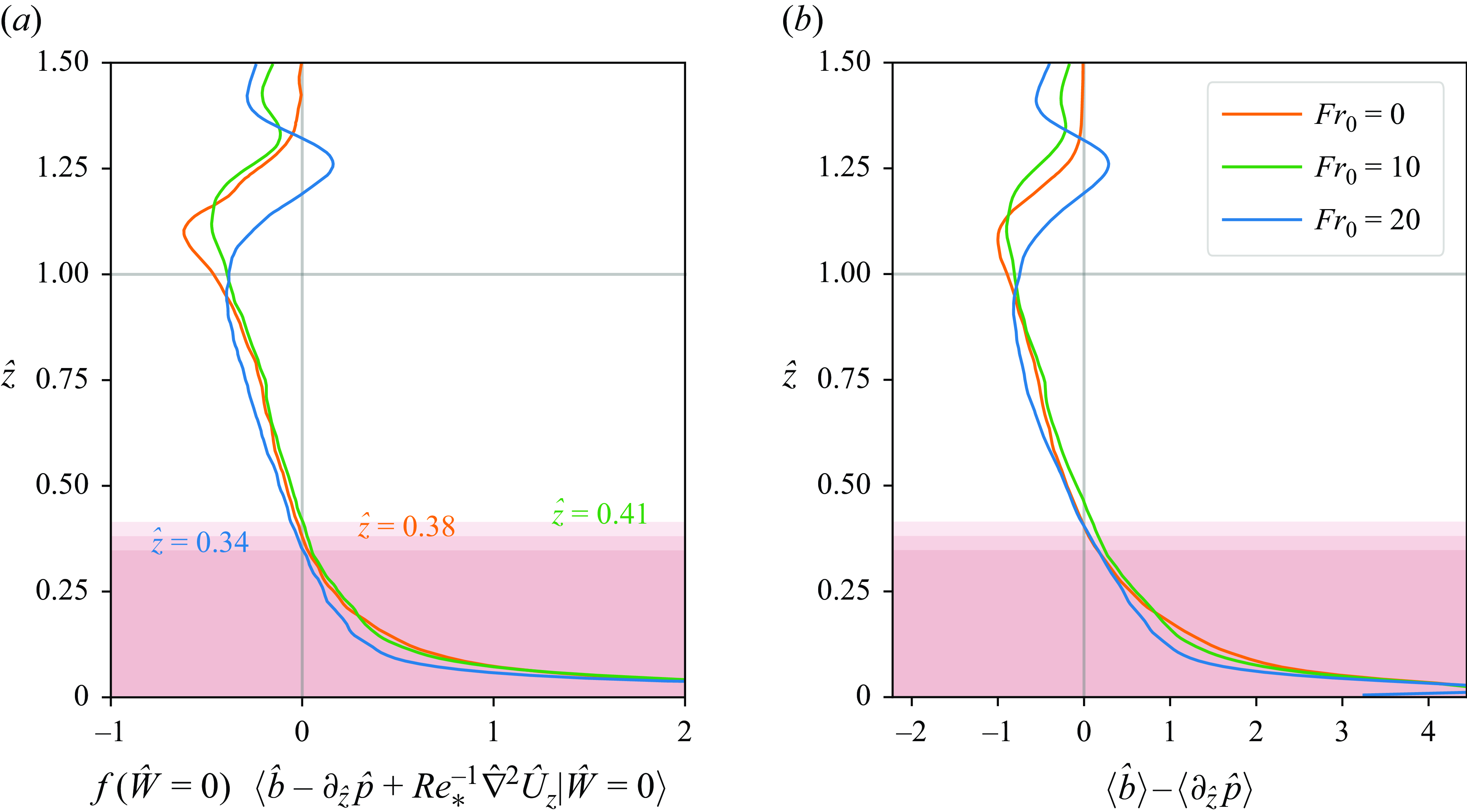
Equation (3.20) shows that the evolution of the area fraction with height is related to a conditional average of the vertical acceleration of a fluid element times the PDF, i.e. the probability flux at $\hat W = 0$
. Figure 10 shows this probability flux for various values of the vertical velocity. Remarkably, the shape of the different contributions does not vary too much with the condition, at least for the range
$\hat W = 0$
. Figure 10 shows this probability flux for various values of the vertical velocity. Remarkably, the shape of the different contributions does not vary too much with the condition, at least for the range $\hat W \in [-0.5,1]$
, as shown in figure 11.
$\hat W \in [-0.5,1]$
, as shown in figure 11.
The right-hand side of (3.20) is plotted in figure 10(a) for different atmospheric conditions. We observe that the right-hand side of (3.20) has a similar profile for different values of the condition $\hat {W}$
when the condition has amplitudes within the bulk of the PDF – see figure 11 for the right-hand side plotted for such values of
$\hat {W}$
when the condition has amplitudes within the bulk of the PDF – see figure 11 for the right-hand side plotted for such values of $\hat {W}$
. Furthermore, we observe that the vertical profile of the right-hand side for the different conditions is similar to the profile of the deviations from the hydrostatic balance,
$\hat {W}$
. Furthermore, we observe that the vertical profile of the right-hand side for the different conditions is similar to the profile of the deviations from the hydrostatic balance, $ ( \langle \hat {b} \rangle - \langle {\partial \hat {p}}/{\partial \hat {z}} \rangle )$
, plotted in figure 10(b). These profiles are in good approximation proportional to each other with a constant of proportionality. When the condition is
$ ( \langle \hat {b} \rangle - \langle {\partial \hat {p}}/{\partial \hat {z}} \rangle )$
, plotted in figure 10(b). These profiles are in good approximation proportional to each other with a constant of proportionality. When the condition is $\hat {W}=0$
, as in (3.20), the constant of proportionality is comparable to the value of
$\hat {W}=0$
, as in (3.20), the constant of proportionality is comparable to the value of $A^+_{\hat {W}}$
in the mixed layer for each CBL. A theoretical explanation for this is still missing.
$A^+_{\hat {W}}$
in the mixed layer for each CBL. A theoretical explanation for this is still missing.
The shaded area of the plots in figure 10 indicates the fraction of the CBL where buoyancy deviations dominate the vertical pressure gradient force. Once a certain height is reached, the vertical pressure gradient force becomes strong enough to dominate buoyancy. Our interpretation of this is that in the lower 30–40 % of the CBL, the heat flux at the surface controls the behaviour of updrafts and downdrafts, and the mass flux between these two, whereas the rest of the mixed layer is pressure dominated. Moreover, at 30–40 % of $z_{{enc}}$
, the mass flux changes from growing with height to decreasing with height, which implies that the mass flux is maximum at 30–40 % of
$z_{{enc}}$
, the mass flux changes from growing with height to decreasing with height, which implies that the mass flux is maximum at 30–40 % of $z_{{enc}}$
. Finally, a significant difference in the behaviour of the mass flux between the different Froude numbers can only be appreciated above
$z_{{enc}}$
. Finally, a significant difference in the behaviour of the mass flux between the different Froude numbers can only be appreciated above $z_{{enc}}$
.
$z_{{enc}}$
.


3.3.1. Area fractions and skewness
The asymmetry of area fractions of updrafts and downdrafts contributes to the characteristic positive skewness on vertical velocity in CBLs. In this subsection, we study such a link of area fractions to the skewness of the vertical velocity PDF. Moeng & Rotunno (Reference Moeng and Rotunno1990) derived an approximation for the skewness of the vertical velocity PDF. They followed a similar decomposition into updrafts and downdrafts for a case of bottom-only heating CBL with a solid wall at the top:
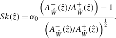 \begin{equation} Sk (\hat {z}) = \alpha _0 \frac {\left (A_{\hat {W}}^-(\hat {z})\Big /A_{\hat {W}}^+(\hat {z})\right )-1}{\left (A_{\hat {W}}^-(\hat {z})\Big /A_{\hat {W}}^+(\hat {z})\right )^{\frac{1}{2}}}. \end{equation}
Figure 12 shows the vertical profile of skewness for both DNS and the Moeng & Rotunno (Reference Moeng and Rotunno1990) approximation for two types of CBLs, one shear-free and one sheared. We choose the parameter $\alpha _0$
for each type of CBL to minimise the mean squared error (MSE) in the shaded area of the plot. The model captures the increase of the skewness with height in the shear-free CBL, which is the condition considered by Moeng & Rotunno (Reference Moeng and Rotunno1990), but the model deviates more in the case of a sheared CBL. Close to the entrainment zone, their approximation does not reproduce the skewness profile of the CBLs that we analyse. This is due to the differences in the geometry of the systems, and to entrainment effects. The CBLs that we analyse relax to a stably stratified free atmosphere, while the boundary layer that they analyse has a solid wall on the top. Moeng & Rotunno (Reference Moeng and Rotunno1990) also see differences between their model and their large-eddy simulations data at the top of their boundary layer, since they cannot reproduce the effects of entrainment. Another difference is that in Moeng & Rotunno (Reference Moeng and Rotunno1990),
$\alpha _0$
for each type of CBL to minimise the mean squared error (MSE) in the shaded area of the plot. The model captures the increase of the skewness with height in the shear-free CBL, which is the condition considered by Moeng & Rotunno (Reference Moeng and Rotunno1990), but the model deviates more in the case of a sheared CBL. Close to the entrainment zone, their approximation does not reproduce the skewness profile of the CBLs that we analyse. This is due to the differences in the geometry of the systems, and to entrainment effects. The CBLs that we analyse relax to a stably stratified free atmosphere, while the boundary layer that they analyse has a solid wall on the top. Moeng & Rotunno (Reference Moeng and Rotunno1990) also see differences between their model and their large-eddy simulations data at the top of their boundary layer, since they cannot reproduce the effects of entrainment. Another difference is that in Moeng & Rotunno (Reference Moeng and Rotunno1990), $\alpha _0 = 2$
for a case of bottom-only heating boundary layer with a solid wall on the top, whereas here we obtain 50–100 % larger values for
$\alpha _0 = 2$
for a case of bottom-only heating boundary layer with a solid wall on the top, whereas here we obtain 50–100 % larger values for $\alpha _0$
, with
$\alpha _0$
, with $\alpha _0 = 3.8$
for a CBL with
$\alpha _0 = 3.8$
for a CBL with $Fr_0 = 20$
and
$Fr_0 = 20$
and ${\textit {Re}}_0 = 42$
, and
${\textit {Re}}_0 = 42$
, and $\alpha _0 = 2.9$
for a CBL with
$\alpha _0 = 2.9$
for a CBL with $Fr_0 = 0$
and
$Fr_0 = 0$
and ${\textit {Re}}_0 = 42$
.
${\textit {Re}}_0 = 42$
.
Vertical profile of skewness for a shear-free boundary layer and a sheared boundary layer. Darker lines represent data from DNS, whereas faded lines correspond to (3.24), the approximation by Moeng & Rotunno (Reference Moeng and Rotunno1990). The parameter $\alpha _0$
is fitted to minimise the mean squared error (MSE) only in the shaded region of the plot.
$\alpha _0$
is fitted to minimise the mean squared error (MSE) only in the shaded region of the plot.
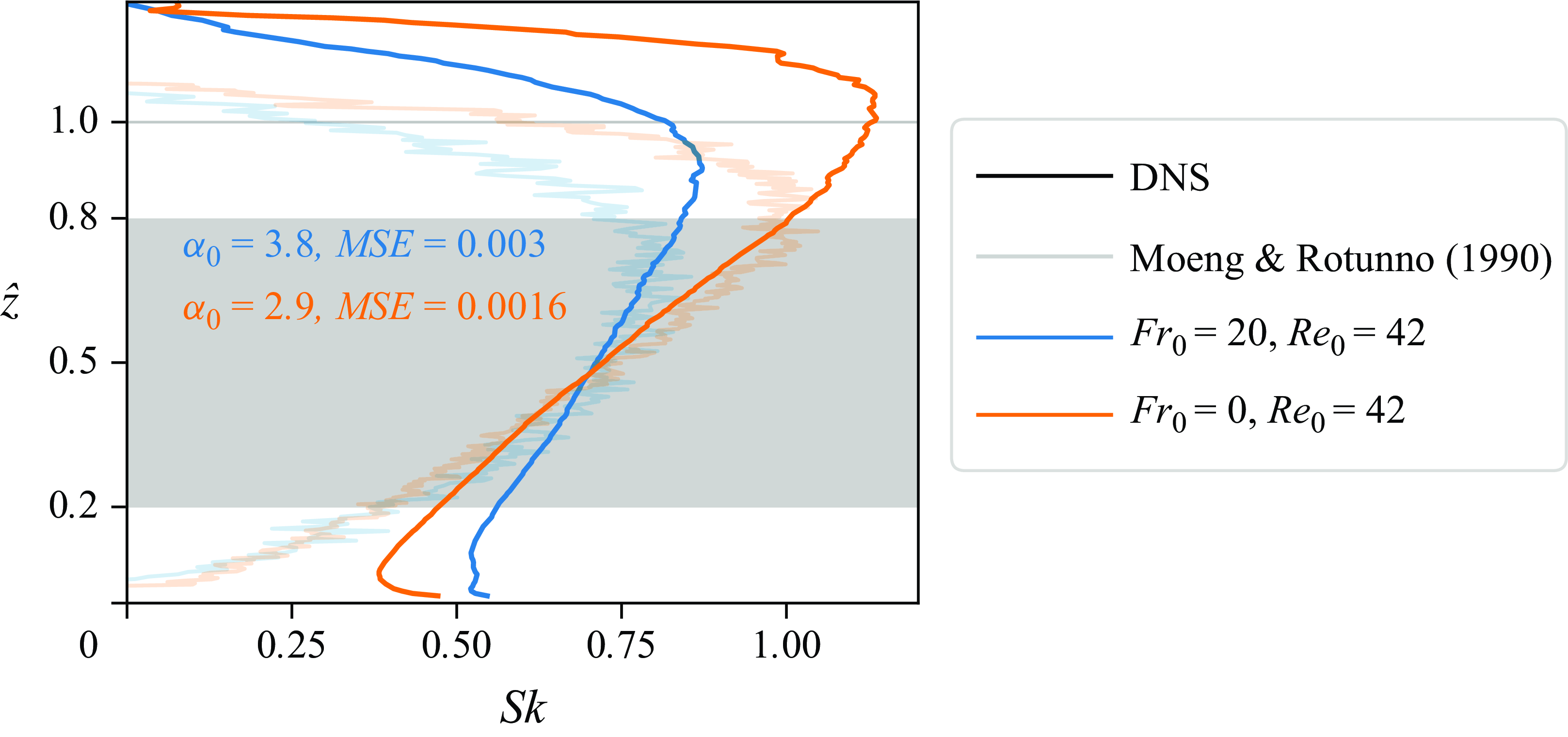
4. Summary and conclusions
We carried out a comprehensive analysis of PDFs of vertical velocity and buoyancy in convective boundary layers. Analysing DNS data in the framework of PDF equations, we studied the height dependence of the single-point single-time PDFs of both quantities. When normalised by convective scales, the temporal evolution of the CBL is scaled out, such that the PDFs are quasi-steady. In terms of their height dependence, as expected, the PDFs show the most significant variations in the surface layer as well as in the entrainment zone. In the well-mixed region, the PDFs approximately collapse at different heights, indicating statistical homogeneity.
The evolution of the PDFs with height can be analysed with the method of characteristics. For the vertical velocity, we find that the statistical evolution following a conditional particle is determined by a complex interplay of buoyancy, vertical pressure gradient force and viscous diffusion that controls the velocity amplitude and thereby also the conditional particle’s evolution in height. For moderate velocity amplitudes, this results in a periodic evolution in the phase space spanned by vertical velocity and height, whereas higher velocity amplitudes also show a flux to and from the upper atmospheric layer (figure 3). For the buoyancy, the major contribution in magnitude is due to thermal diffusion.
Regarding the statistical evolution of buoyancy fluctuations in height, as expected, the vertical velocity conditioned on $\hat {\theta }$
close to the bottom is positive for positively buoyant fluid elements, whereas it tends to be negative for negatively buoyant fluid elements. In the entrainment layer, the conditional velocity can be negative even for positively buoyant fluid elements, which indicates the entrainment of buoyant fluid from the free atmosphere into the boundary layer. In the phase space spanned by buoyancy and height, the characteristics reflect two patterns of circular motion for a conditional particle (figure 7). One pattern is localised in the mixed layer where conditional particles with higher buoyancy rise while losing buoyancy, before sinking once their buoyancy decreases enough. A secondary pattern is localised in the entrainment zone and caused by the entrainment of buoyant conditional particles from the upper layers into the CBL, resulting also in significant variations in the PDF of buoyancy in this region. This secondary pattern is absent in the mean evolution of the vertical velocity of fluid parcels, which tend to penetrate further into the entrainment zone.
$\hat {\theta }$
close to the bottom is positive for positively buoyant fluid elements, whereas it tends to be negative for negatively buoyant fluid elements. In the entrainment layer, the conditional velocity can be negative even for positively buoyant fluid elements, which indicates the entrainment of buoyant fluid from the free atmosphere into the boundary layer. In the phase space spanned by buoyancy and height, the characteristics reflect two patterns of circular motion for a conditional particle (figure 7). One pattern is localised in the mixed layer where conditional particles with higher buoyancy rise while losing buoyancy, before sinking once their buoyancy decreases enough. A secondary pattern is localised in the entrainment zone and caused by the entrainment of buoyant conditional particles from the upper layers into the CBL, resulting also in significant variations in the PDF of buoyancy in this region. This secondary pattern is absent in the mean evolution of the vertical velocity of fluid parcels, which tend to penetrate further into the entrainment zone.
It is interesting to compare the buoyancy statistics in CBLs to the temperature statistics in RBC, which has been investigated previously by Lülff et al. (Reference Lülff, Wilczek and Friedrich2011, Reference Lülff, Wilczek, Stevens, Friedrich and Lohse2015). The CBL and RBC cases share several similarities, including, for example, the faster upward movement of buoyant (hot) fluid compared to non-buoyant (cold) fluid in the lower half of the convection system, and the fact that the main heating/cooling movements are located near the boundaries (bottom for CBL, and bottom and top for RBC). An important difference between CBL and RBC is that CBLs lack the top–bottom symmetry present in RBC due to the different roles of bottom boundary and the entrainment zone. As a result, the secondary circulation pattern observed for the CBL buoyancy is absent in RBC.
Furthermore, we extended the analysis to the study of the area fractions of the different updraft, downdraft, buoyant and non-buoyant contributions to the PDFs that we analysed, and to the study of a set of equations for the mass flux. We observe that the mass flux between updrafts and downdrafts has a profile similar to that of the deviations from the hydrostatic balance, and that the mass flux is maximum at 30–40 % of $z_{{enc}}$
for sheared and purely convective cases. Mass flux equations provide a quantitative understanding of the vertical exchange of air mass in the CBL, therefore these results can help as reference to assess mass flux parametrisations used in weather and climate models.
$z_{{enc}}$
for sheared and purely convective cases. Mass flux equations provide a quantitative understanding of the vertical exchange of air mass in the CBL, therefore these results can help as reference to assess mass flux parametrisations used in weather and climate models.
Acknowledgements
This work was supported by the Fraunhofer–Max Planck Cooperation Program through the TWISTER project. V.C.M. gratefully acknowledges the support by a fellowship of the International Max Planck Research School (IMPRS) for Physics of Biological and Complex Systems. The authors gratefully acknowledge the Gauss Centre for Supercomputing e.V. (www.gauss-centre.eu) for funding this project by providing computing time through the John von Neumann Institute for Computing (NIC) on the GCS Supercomputer JUWELS at Jülich Supercomputing Centre (JSC).
Declaration of interests
The authors report no conflict of interest.
Appendix A. Mixed-layer similarity and PDF rescaling
In this appendix, we verify the so-called mixed-layer similarity (Wyngaard Reference Wyngaard2010) with the help of DNS data. Within the mixed layer, vertical velocity and buoyancy are approximately self-similar in time, characterised by the convective scales defined in (2.7) and (2.8). Following a proper scaling given by (3.4) and (3.12), the PDF for vertical velocity and buoyancy can be collapsed as shown in figure 13. This asymptotic behaviour occurs once a free-convection-like state emerges (Wyngaard Reference Wyngaard2010). It is within this state that the CBL reaches the so-called mixed-layer similarity. Also within this state, and when non-dimensionalised with the convective scales, vertical velocity and buoyancy become functions of $z/z_{{enc}}$
only.
$z/z_{{enc}}$
only.


Appendix B. The PDF evolution equation
In this appendix, we derive the evolution equation for the PDF of $f(W,\theta ;z,t)$
. This derivation is based on Pope (Reference Pope1981, Reference Pope1985, 2000), and uses properties of the fine-grained PDF.
$f(W,\theta ;z,t)$
. This derivation is based on Pope (Reference Pope1981, Reference Pope1985, 2000), and uses properties of the fine-grained PDF.
The fine-grained PDF of vertical velocity and buoyancy is
 \begin{equation} f^{\prime}(W,\theta ; \boldsymbol x,t) = \delta \left ( U_z(\boldsymbol x,t) - W \right )\, \delta \left ( b(\boldsymbol x,t) - \theta \right ) \end{equation}
for a given realisation of the flow. At each point $\boldsymbol x$
and time
$\boldsymbol x$
and time $t$
,
$t$
, $f^{\prime}$
is a two-dimensional delta function in the vertical velocity and buoyancy space. The PDF is then defined as
$f^{\prime}$
is a two-dimensional delta function in the vertical velocity and buoyancy space. The PDF is then defined as
 \begin{equation} f(W,\theta ;z,t) = \langle f^{\prime}(W,\theta ;\boldsymbol x,t) \rangle . \end{equation}
Due to homogeneity in horizontal directions, the PDF depends on $(z,t)$
only. The conditional average of some function
$(z,t)$
only. The conditional average of some function $\phi$
can be introduced as
$\phi$
can be introduced as
 \begin{equation} \langle \phi (\boldsymbol x,t)\, f^{\prime}(W,\theta ;\boldsymbol x,t) \rangle = \langle \phi (\boldsymbol x,t) \,|\, W,\theta ; z, t\rangle\, f(W,\theta ;z,t) . \end{equation}
Furthermore, the temporal and spatial derivatives of $f^{\prime}(W,\theta ;\boldsymbol x,t)$
are
$f^{\prime}(W,\theta ;\boldsymbol x,t)$
are
 \begin{equation} \frac {\partial }{\partial t} f^{\prime}(W,\theta ;\boldsymbol x,t) = - \frac {\partial }{\partial W} f^{\prime}(W,\theta ;\boldsymbol x,t)\, \frac {\partial }{\partial t} U_z(\boldsymbol x,t) - \frac {\partial }{\partial \theta } f^{\prime}(W,\theta ;\boldsymbol x,t)\,\frac {\partial }{\partial t} b(\boldsymbol x,t) \end{equation}
and
 \begin{equation} \frac {\partial }{\partial z} f^{\prime}(W,\theta ;\boldsymbol x,t) = - \frac {\partial }{\partial W} f^{\prime}(W,\theta ;\boldsymbol x,t)\, \frac {\partial }{\partial z} U_z(\boldsymbol x,t) - \frac {\partial }{\partial \theta } f^{\prime}(W,\theta ;\boldsymbol x,t)\,\frac {\partial }{\partial z} b(\boldsymbol x,t). \end{equation}
The partial derivatives with respect to $x$
and
$x$
and $y$
are obtained analogously. Another important result required in this derivation is
$y$
are obtained analogously. Another important result required in this derivation is
 \begin{equation} \boldsymbol U(\boldsymbol x,t) {\boldsymbol \cdot } \nabla f^{\prime}(W,\theta ;\boldsymbol x,t) = \boldsymbol V {\boldsymbol \cdot } \nabla f^{\prime}(W,\theta ;\boldsymbol x,t). \end{equation}
Here, $\boldsymbol V = (U,V,W)$
is the sample-space vector corresponding to the velocity field
$\boldsymbol V = (U,V,W)$
is the sample-space vector corresponding to the velocity field $\boldsymbol U =(U_x,U_y,U_z)$
. For this, we used the incompressibility of the fluid, the sifting property of the delta function, and the fact that
$\boldsymbol U =(U_x,U_y,U_z)$
. For this, we used the incompressibility of the fluid, the sifting property of the delta function, and the fact that $\boldsymbol V$
is an independent variable.
$\boldsymbol V$
is an independent variable.
Hence the total derivative of $f^{\prime}(W,\theta ;\boldsymbol x,t)$
is
$f^{\prime}(W,\theta ;\boldsymbol x,t)$
is
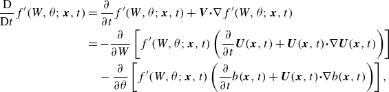 \begin{align} \frac {{\rm D}}{{\rm D}t} f^{\prime}(W,\theta ;\boldsymbol x,t) &= \frac {\partial }{\partial t} f^{\prime}(W,\theta ;\boldsymbol x,t) + \boldsymbol V {\boldsymbol \cdot } \nabla f^{\prime}(W,\theta ;\boldsymbol x,t) \notag\\ &= - \frac {\partial }{\partial W} \left [ f^{\prime}(W,\theta ;\boldsymbol x,t) \left ( \frac {\partial }{\partial t} \boldsymbol U(\boldsymbol x,t) + \boldsymbol U(\boldsymbol x,t) {\boldsymbol \cdot } \nabla \boldsymbol U(\boldsymbol x,t)\right ) \right ] \notag\\ & \quad - \frac {\partial }{\partial \theta } \left [ f^{\prime}(W,\theta ; \boldsymbol x,t) \left ( \frac {\partial }{\partial t} b(\boldsymbol x,t) + \boldsymbol U(\boldsymbol x,t) {\boldsymbol \cdot } \nabla b(\boldsymbol x,t)\right ) \right ], \end{align}
and the mean of this equation yields the PDF equation
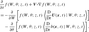 \begin{align} &\frac {\partial }{\partial t} f(W,\theta ;z,t) + \boldsymbol V {\boldsymbol \cdot } \nabla f(W,\theta ;z,t) \notag\\ &= - \frac {\partial }{\partial W} \left [ f(W,\theta ;z,t) \,\left \langle \frac {{\rm D}}{{\rm D}t} \boldsymbol U(\boldsymbol x,t) \,\Big |\, W,\theta ;z,t \right \rangle \right ]\notag\\ &\quad - \frac {\partial }{\partial \theta } \left [ f(W,\theta ;z,t)\, \left \langle \frac {{\rm D}}{{\rm D}t} b(\boldsymbol x,t) \,\Big |\, W,\theta ;z,t \right \rangle \right ]. \end{align}
Finally, we substitute the equations of motion (2.1) into the previous equation such that, after considering horizontal homogeneity, we obtain the evolution equation for the PDF of vertical velocity and buoyancy:
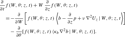 \begin{align} &\frac {\partial }{\partial t} f(W,\theta ;z,t) + W\, \frac {\partial }{\partial z} f(W,\theta ;z,t) \nonumber\\ &\quad = - \frac {\partial }{\partial W} \left [ f(W,\theta ;z,t)\,\left \langle b - \frac {\partial }{\partial z} p + \nu\, \nabla ^2 U_z \,\Big |\, W, \theta ;z,t \right \rangle \right ]\nonumber\\ &\qquad- \frac {\partial }{\partial \theta } [ f(W,\theta ;z,t)\, \langle \kappa _b\, \nabla ^2 \textit {b}\, |\,W, \theta ;z,t \rangle ]. \end{align}
Appendix C. Normal Reynolds stress
The transport equations for the Reynolds stresses, especially in the normal direction, are particularly interesting when studying CBLs. The flow in a CBL is statistically homogeneous in the streamwise and spanwise directions. Hence, just as in a fully developed channel flow (Mansour et al. Reference Mansour, Kim and Moin1988), the relevant non-zero components of the Reynolds stresses are $\langle u^{\prime 2}_z \rangle$
and
$\langle u^{\prime 2}_z \rangle$
and $\langle u^{\prime}_z u^{\prime}_x \rangle$
. Let us focus on the former. After multiplying (3.5) by the velocity fluctuations squared
$\langle u^{\prime}_z u^{\prime}_x \rangle$
. Let us focus on the former. After multiplying (3.5) by the velocity fluctuations squared $(\hat {W}-\langle \hat {U}_z \rangle )^2$
, and integrating over the velocity space, we obtain the evolution equation for the normal Reynolds stress. If we further consider that
$(\hat {W}-\langle \hat {U}_z \rangle )^2$
, and integrating over the velocity space, we obtain the evolution equation for the normal Reynolds stress. If we further consider that $\langle \hat {U}_z \rangle \approx 0$
, then the equation simplifies to
$\langle \hat {U}_z \rangle \approx 0$
, then the equation simplifies to
 \begin{equation} \frac {\partial }{\partial \hat {z}} \langle u^{\prime 3}_z \rangle = 2 \langle u^{\prime}_z \hat {b}' \rangle - 2 \left \langle u^{\prime}_z\, \frac {\partial }{\partial \hat {z}} \hat {p} '\right \rangle + 2\, {\textit {Re}}_*^{-1}\, \langle u^{\prime}_z\, \hat \nabla ^2 u^{\prime}_z \rangle - \frac {1}{3\hat {t}} \langle u^{\prime 2}_z \rangle . \end{equation}
The term on the left-hand side represents the turbulent transport. On the right, the first term, which is directly linked to the buoyancy fluctuations, refers to the heat flux; then follows a term representing the pressure redistribution, then the dissipation, and finally a term containing $\langle u^{\prime 2}_z \rangle$
. Note that the coefficient for the latter term can also be expressed as
$\langle u^{\prime 2}_z \rangle$
. Note that the coefficient for the latter term can also be expressed as $ ({t_*}/{w_*})\, {\partial w_*^2}/{\partial t}$
. This last term indicates the contribution of the convective scales and their time dependence to the equation for the Reynolds stresses when considering the standardised version of them. Furthermore, due to
$ ({t_*}/{w_*})\, {\partial w_*^2}/{\partial t}$
. This last term indicates the contribution of the convective scales and their time dependence to the equation for the Reynolds stresses when considering the standardised version of them. Furthermore, due to $\langle \hat {U}_z \rangle \approx 0$
, the normal Reynolds stress has no source term or mean flow advection term.
$\langle \hat {U}_z \rangle \approx 0$
, the normal Reynolds stress has no source term or mean flow advection term.
Using data from our DNS, we analysed and plotted each term of (C1); see figure 14. The heat flux is the dominant source term in most of the CBL until its zero crossing when $z=z_{{enc}}$
. The pressure transport is the dominant sink term except close to the wall, where dissipation dominates. This previous statement is true for all the CBLs analysed here, except for the shear-free case, in which the pressure term dominates as loss term even close to the wall. The quasi-steady term that comes from the standardisation of the equation with the convective scales is negligible everywhere. The heat flux combined with the pressure transport, the dissipation term and the quasi-steady term coming from the scaling add up to account for the turbulent advection on the left-hand side of the equation.
$z=z_{{enc}}$
. The pressure transport is the dominant sink term except close to the wall, where dissipation dominates. This previous statement is true for all the CBLs analysed here, except for the shear-free case, in which the pressure term dominates as loss term even close to the wall. The quasi-steady term that comes from the standardisation of the equation with the convective scales is negligible everywhere. The heat flux combined with the pressure transport, the dissipation term and the quasi-steady term coming from the scaling add up to account for the turbulent advection on the left-hand side of the equation.
Terms in the budget of $\langle u^{\prime 2}_z \rangle$
. The different curves represent the different terms in (C1) for a CBL with
$\langle u^{\prime 2}_z \rangle$
. The different curves represent the different terms in (C1) for a CBL with ${\textit {Re}}_0 = 45$
and
${\textit {Re}}_0 = 45$
and $Fr_0 = 20$
.
$Fr_0 = 20$
.
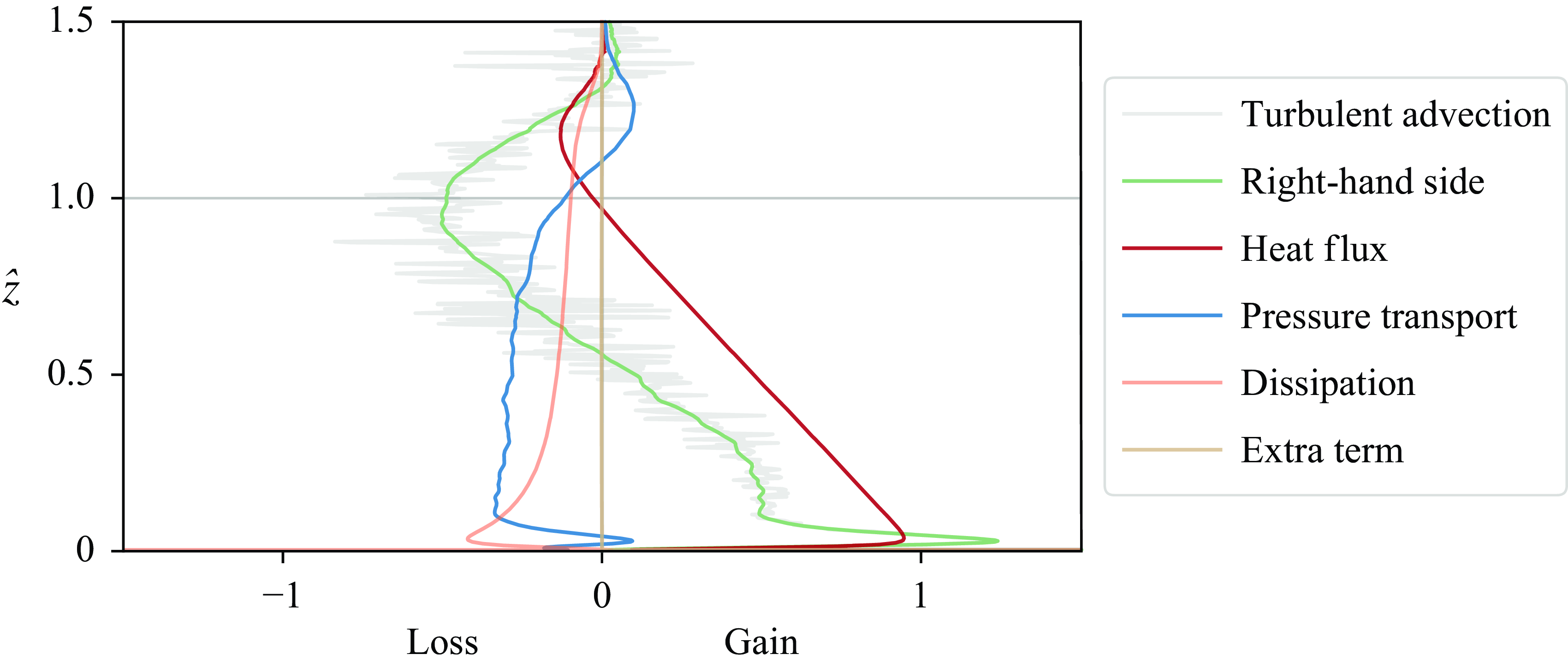
If we consider the budget of a fully developed channel flow, where streamwise and spanwise directions are also homogeneous, we can directly compare the relevant non-zero stresses $\langle u^{\prime 2}_z \rangle$
of both cases, channel flow and CBL, term by term against each other; see e.g. figure 2 of Mansour et al. (Reference Mansour, Kim and Moin1988). Just as in the CBL case, the budget does not have an explicit forcing term as source term; nonetheless, contrary to a CBL where the heat flux is the dominant source term, for a channel flow the pressure transport is the dominant source term. For a channel flow, the dissipation rate is the dominant sink term; for a CBL, while dissipation is still consuming, it is not dominant. For both cases, the turbulent advection (left-hand side of the budget equation) is of the same order of the rest of the terms on the right-hand side.
$\langle u^{\prime 2}_z \rangle$
of both cases, channel flow and CBL, term by term against each other; see e.g. figure 2 of Mansour et al. (Reference Mansour, Kim and Moin1988). Just as in the CBL case, the budget does not have an explicit forcing term as source term; nonetheless, contrary to a CBL where the heat flux is the dominant source term, for a channel flow the pressure transport is the dominant source term. For a channel flow, the dissipation rate is the dominant sink term; for a CBL, while dissipation is still consuming, it is not dominant. For both cases, the turbulent advection (left-hand side of the budget equation) is of the same order of the rest of the terms on the right-hand side.
To understand the main difference between these two budgets – the role of the pressure transport term– we must refer to an essential difference between these two physical systems: their influx of momentum. While the channel flow receives its intake of momentum in the streamwise direction, the CBL does so in the vertical direction at its lower boundary by means of the surface buoyancy flux $B_0$
. Hence the budget for
$B_0$
. Hence the budget for $\langle u^{\prime 2}_z \rangle$
in the channel flow does not have a source term per se, but the vertical velocity pressure gradient term is the dominant source (redistribution) term that brings momentum from the spanwise direction to the vertical direction. Compared to that, the budget for the CBL does not have a source term either, and its dominant source term is the heat flux, while this time, the velocity pressure gradient term redistributes energy from the vertical direction to the streamwise direction.
$\langle u^{\prime 2}_z \rangle$
in the channel flow does not have a source term per se, but the vertical velocity pressure gradient term is the dominant source (redistribution) term that brings momentum from the spanwise direction to the vertical direction. Compared to that, the budget for the CBL does not have a source term either, and its dominant source term is the heat flux, while this time, the velocity pressure gradient term redistributes energy from the vertical direction to the streamwise direction.
C.1. Evolution equation
One of the advantages of working with PDF methods is that equations for the evolution of the moment of the PDF can be derived straightforwardly. In particular, the second moment of $f(W)$
represents the normal Reynolds stress. To obtain the evolution equation for the normal Reynolds stress, we multiply (3.3) by
$f(W)$
represents the normal Reynolds stress. To obtain the evolution equation for the normal Reynolds stress, we multiply (3.3) by $W^2$
(which approximately equals the squared fluctuations since
$W^2$
(which approximately equals the squared fluctuations since $\langle U_z \rangle \approx 0$
) and integrate over the velocity space.
$\langle U_z \rangle \approx 0$
) and integrate over the velocity space.
Starting from the left-hand side, term by term this results in
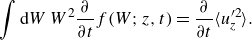 \begin{equation} \int {\rm d}W\, W^2 \frac {\partial }{\partial t}f(W;z,t) = \frac {\partial }{\partial t} \langle u^{\prime 2}_z\rangle . \end{equation}
The advective term yields
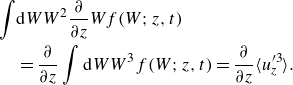 \begin{align} \int &{\rm d}W W^2 \frac {\partial }{\partial z}W f(W;z,t) \nonumber\\ &=\frac {\partial }{\partial z} \int {\rm d}W W^3 f(W; z,t) = \frac {\partial }{\partial z} \langle u^{\prime 3}_z\rangle. \end{align}
For the right-hand side, the first term results in
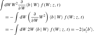 \begin{align} \int &{\rm d}W W^2 \frac {\partial }{\partial W} \langle b \,|\, W \rangle\, f(W;z,t) \nonumber \\& = - \int {\rm d}W \left ( \frac {\partial }{\partial W} W^2 \right ) \langle b \,|\, W \rangle\, f(W;z,t) \nonumber \\&=- \int {\rm d}W\, 2 W \, \langle b \,|\, W \rangle\, f(W;z,t) = -2\langle u^{\prime}_zb'\rangle . \end{align}
The rest of the terms on the right-hand side are derived in a similar way. Hence the full equation takes the form
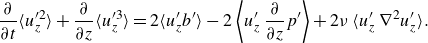 \begin{equation} \frac {\partial }{\partial t} \langle u^{\prime 2}_z\rangle + \frac {\partial }{\partial z} \langle u^{\prime 3}_z \rangle = 2 \langle u^{\prime}_z b' \rangle - 2 \left \langle u^{\prime}_z\, \frac {\partial }{\partial z} p '\right \rangle + 2 \nu\, \langle u^{\prime}_z\, \nabla ^2 u^{\prime}_z \rangle . \end{equation}
Naturally, it is also possible to obtain such an equation from the PDF for normalised variables, (3.5), and thus recover (C1) directly. In particular. the quasi-steady term is
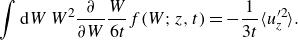 \begin{equation} \int {\rm d}W\, W^2 \frac {\partial }{\partial W} \frac {W}{6t} f(W;z,t) = - \frac {1}{3t} \langle u^{\prime 2}_z \rangle . \end{equation}
It is also possible to recover (C1) from (C5) by normalising the former with the convective scales. For example:
 \begin{equation} \frac {\partial }{\partial t} \langle u^{\prime 2}_z \rangle = \frac {\partial }{\partial t} w_*^2 \langle \hat {u}^{\prime 2} _z \rangle = w_*^2 \frac {\partial }{\partial t} \langle \hat {u}^{\prime 2} _z \rangle + \langle \hat {u}^{\prime 2} _z \rangle \frac {\partial }{\partial t} w_*^2 = w_*^2 \frac {\partial }{\partial t} \langle \hat {u}^{\prime 2} _z \rangle + \langle \hat {u}^{\prime 2} _z \rangle \left ( \frac {w_*^2}{3 t} \right ). \end{equation}
After removing dimensions and considering the quasi-stationary state, one recovers the last term in (C1).


 Open access