


1. Introduction
The Saffman–Taylor instability (Saffman & Taylor Reference Saffman and Taylor1958; Chuoke, van Meurs & van der Poel Reference Chuoke, van Meurs and van der Poel1959) occurs when a lower viscosity fluid displaces a more viscous fluid. The interface between the two fluids becomes hydrodynamically unstable due to the unfavourable viscosity contrast, forming a finger-like pattern, referred to as viscous fingering (VF) – comprehensive reviews can be referred to (Homsy Reference Homsy1987; McCloud & Maher Reference McCloud and Maher1995). This instability is highly relevant to the applications in enhanced oil recovery (Homsy Reference Homsy1987; Faisal et al. Reference Faisal, Chevalier, Bernabe, Juanes and Sassi2015; Fu et al. Reference Fu, Cueto-Felgueroso, Bolster and Juanes2015), chromatography (Broyles et al. Reference Broyles, Shalliker, Cherrak and Guiochon1998), gastric acid transport processes (Bhaskar et al. Reference Bhaskar, Garik, Turner, Bradley, Bansil, Stanley and LaMont1992) and carbon capture and storage (CCS) (Orr & Taber Reference Orr and Taber1984; Orr Reference Orr2009; Huppert & Neufeld Reference Huppert and Neufeld2014; Li et al. Reference Li, Lin, Cai, Chen and Meiburg2023). Because of the mathematical similarity of the Darcy equation in a porous medium and the Hele-Shaw equation in two parallel plates, VF in a Hele-Shaw cell is often studied in lieu of the opaque porous media flows. Viscous fingering has been a subject of thorough study both experimentally and numerically for many decades. The configurations investigated mainly consist of three geometries: the rectilinear displacement (De Wit & Homsy Reference De Wit and Homsy1999a,Reference De Wit and Homsyb; Jha, Cueto-Felgueroso & Juanes Reference Jha, Cueto-Felgueroso and Juanes2011); the radial injection (Li et al. Reference Li, Lowengrub, Fontana and Palffy-Muhoray2009; Chen et al. Reference Chen, Huang, Wang and Miranda2010; Dias et al. Reference Dias, Alvarez-Lacalle, Carvalho and Miranda2012; Yuan & Azaiez Reference Yuan and Azaiez2014; Huang & Chen Reference Huang and Chen2015; Tsuzuki et al. Reference Tsuzuki, Li, Nagatsu and Chen2019b; Verma, Sharma & Mishra Reference Verma, Sharma and Mishra2022); the so-called quarter-five-spot configuration (Chen & Meiburg Reference Chen and Meiburg1998a,Reference Chen and Meiburgb; Petitjeans et al. Reference Petitjeans, Chen, Meiburg and Maxworthy1999). Generally, VF is determined by two factors: viscosity contrast and miscibility. The miscibility is conventionally classified into miscible and immiscible (Homsy Reference Homsy1987). Diffusion occurs in a miscible condition and is treated as a stabilizing factor for VF. On the other hand, in an immiscible condition, interfacial tension is considered a stabilizing factor. To manipulate the interface, variants of flow fields by changing the physical conditions are commonly investigated and proposed, such as time-dependent injection (Li et al. Reference Li, Lowengrub, Fontana and Palffy-Muhoray2009; Chen et al. Reference Chen, Huang, Wang and Miranda2010; Dias et al. Reference Dias, Alvarez-Lacalle, Carvalho and Miranda2012; Yuan & Azaiez Reference Yuan and Azaiez2014), cell rotation (Carrillo et al. Reference Carrillo, Magdaleno, Casademunt and Ortín1996; Chen, Huang & Miranda Reference Chen, Huang and Miranda2011), suction flow (Thomé et al. Reference Thomé, Rabaud, Hakim and Couder1989; Chen, Huang & Miranda Reference Chen, Huang and Miranda2014), cell lifting (Shelley, Tian & Wlodarski Reference Shelley, Tian and Wlodarski1997; Chen, Chen & Miranda Reference Chen, Chen and Miranda2005) and injection alternation (Jha et al. Reference Jha, Cueto-Felgueroso and Juanes2011; Chen et al. Reference Chen, Huang, Huang and Miranda2015; Chou, Huang & Chen Reference Chou, Huang and Chen2023). In addition, another effective means to control the interface is modifying the physical properties at the fluid–fluid interface by inducing chemical reactions. A popular method is to vary the local viscosity at the interface by reaction (Nagatsu et al. Reference Nagatsu, Matsuda, Kato and Tada2007; Gerard & De Wit Reference Gerard and De Wit2009; Hejazi & Azaiez Reference Hejazi and Azaiez2010; Nagatsu et al. Reference Nagatsu, Kondo, Kato and Tada2011; Alhumade & Azaiez Reference Alhumade and Azaiez2013; Stewart et al. Reference Stewart, Marin, Tullier, Pojman, Meiburg and Bunton2018; Sharma et al. Reference Sharma, Pramanik, Chen and Mishra2019). Alternatively, changes of interfacial tension by the production of surfactants are also applied to control the fingering instability (Nasr-El-Din et al. Reference Nasr-El-Din, Khulbe, Hornof and Neale1990; Hornof & Bernard Reference Hornof and Bernard1992; Hornof & Baig Reference Hornof and Baig1995; Hornof, Neale & Gholam-Hosseini Reference Hornof, Neale and Gholam-Hosseini2000; Fernandez & Homsy Reference Fernandez and Homsy2003; Tsuzuki et al. Reference Tsuzuki, Ban, Fujimura and Nagatsu2019a,Reference Tsuzuki, Li, Nagatsu and Chenb). Recent advances in chemical-induced instability are reviewed by De Wit (Reference De Wit2020).
In recent years, a new category called partially miscible systems has been studied in VF (Amooie, Soltanian & Moortgat Reference Amooie, Soltanian and Moortgat2017; Fu, Cueto-Felgueroso & Juanes Reference Fu, Cueto-Felgueroso and Juanes2017; Suzuki et al. Reference Suzuki, Nagatsu, Mishra and Ban2019, Reference Suzuki, Nagatsu, Mishra and Ban2020, Reference Suzuki, Kobayashi, Nagatsu and Ban2021a,Reference Suzuki, Tada, Hirano, Ban, Mishra, Takeda and Nagatsub; Li et al. Reference Li, Cai, Chen and Meiburg2022; Seya et al. Reference Seya, Suzuki, Nagatsu, Ban and Mishra2022; Iwasaki et al. Reference Iwasaki, Nagatsu, Ban, Iijima, Mishra and Suzuki2023; Kim et al. Reference Kim, Palodhi, Hong and Mishra2023). The miscibility is related to solubility. In fully miscible systems, two fluids or two solutions are completely mixed with infinite solubility and finally become one phase. In immiscible systems, two fluids or two solutions do not mix, i.e. zero solubility, and remain in the two separated phases, where the final composition of the two phases is the same as the initial one. In partially miscible systems, two fluids or two solutions mix with finite solubility and become two phases, where the final composition of the two phases is different from the initial one. Partially miscible systems can be further classified into two types. In the first type, only one fluid or solution dissolves in another fluid or solution with finite solubility. In the second type, two fluids or solutions dissolve in each other with finite solubility. In other words, in the second type, the mixed species undergo phase separation to form two new phases. The VF in the partially miscible system is significant in high-temperature and high-pressure processes such as enhanced oil recovery (Faisal et al. Reference Faisal, Chevalier, Bernabe, Juanes and Sassi2015; Fu et al. Reference Fu, Cueto-Felgueroso, Bolster and Juanes2015) and CCS technology (Orr & Taber Reference Orr and Taber1984; Orr Reference Orr2009; Huppert & Neufeld Reference Huppert and Neufeld2014; Li et al. Reference Li, Lin, Cai, Chen and Meiburg2023). The first type may occur in the process of CCS, in which the injected CO $_2$ is in a supercritical state. The solubility of supercritical CO $_2$ and the underground brine is only approximately 5 % (Li et al. Reference Li, Cai, Chen and Meiburg2022). Thus, the conventional treatments of fully miscible or immiscible conditions cannot capture the interfacial phenomena accurately (Fu et al. Reference Fu, Cueto-Felgueroso and Juanes2017; Li et al. Reference Li, Cai, Chen and Meiburg2022, Reference Li, Lin, Cai, Chen and Meiburg2023). In the second type, based on the experimental observations in a radial Hele-Shaw flow, new interfacial patterns triggered by the coupled effect of hydrodynamic VF and thermodynamic phase separation are presented (Suzuki et al. Reference Suzuki, Nagatsu, Mishra and Ban2019, Reference Suzuki, Nagatsu, Mishra and Ban2020, Reference Suzuki, Kobayashi, Nagatsu and Ban2021a,Reference Suzuki, Tada, Hirano, Ban, Mishra, Takeda and Nagatsub). Relevant numerical studies coupling VF and phase separation in a rectilinear geometry are also carried out (Seya et al. Reference Seya, Suzuki, Nagatsu, Ban and Mishra2022; Kim et al. Reference Kim, Palodhi, Hong and Mishra2023). Formation of the droplets is observed both in experiments and simulations, in which the characteristics of interfacial instability are distinct from the conventional VF. The droplet formation caused by the additional thermodynamic effect of phase separation is discussed in two regions: the region of spinodal decomposition and the metastable region. In the spinodal region, where the second derivative of the free energy is negative, the mixture undergoes spontaneous phase separation, forming droplets (Suzuki et al. Reference Suzuki, Nagatsu, Mishra and Ban2020). On the other hand, in the metastable region, where the second derivative of the free energy is positive, phase separation occurs only when subjected to sufficiently strong disturbance. Therefore, while no droplets are formed in experiments, unique fingering shapes characterized by a slim finger root are observed, which is referred to as tip-widening (Suzuki et al. Reference Suzuki, Tada, Hirano, Ban, Mishra, Takeda and Nagatsu2021b). Nevertheless, the mechanism for these tip-widening fingers observed in the metastable region was not sufficiently provided.
The existing studies of phase separation coupling with VF are mainly experimental works. Even though a couple of numerical works have been reported (Seya et al. Reference Seya, Suzuki, Nagatsu, Ban and Mishra2022; Kim et al. Reference Kim, Palodhi, Hong and Mishra2023), no simulations are performed to thoroughly reproduce patterns in a radial Hele-Shaw flow, which can better represent the conditions in the experiments. Besides, all the previous experimental (Suzuki et al. Reference Suzuki, Nagatsu, Mishra and Ban2019, Reference Suzuki, Nagatsu, Mishra and Ban2020, Reference Suzuki, Kobayashi, Nagatsu and Ban2021a,Reference Suzuki, Tada, Hirano, Ban, Mishra, Takeda and Nagatsub) and numerical (Seya et al. Reference Seya, Suzuki, Nagatsu, Ban and Mishra2022; Kim et al. Reference Kim, Palodhi, Hong and Mishra2023) studies focused on the case where phase separation occurs in the interfacial region. In the present study, we conduct the first direct numerical simulations in partially miscible systems in a radial geometry. In addition, the present study focuses on a distinct case in which the injected fluid can undergo spinodal decomposition to understand the coupling between phase separation and VF more comprehensively. Such simulations can provide detailed concentration distributions, which are hard to obtain in experiments, and how the two separation regions, i.e. spinodal and metastable regions, affect the pattern formation. This situation, in which injection fluid (or solution) can undergo spinodal decomposition, is practically possible when the temperature and pressure conditions during the preparation of the injected fluid differ from those during the injection. For instance, the injected fluid (solution) is one phase under the temperature and pressure conditions during preparation, while its composition would undergo spinodal decomposition under the temperature and pressure conditions during injection and mixing.
Notably, the unique patterns associated with phase separations observed in experiments (Suzuki et al. Reference Suzuki, Nagatsu, Mishra and Ban2020, Reference Suzuki, Kobayashi, Nagatsu and Ban2021a,Reference Suzuki, Tada, Hirano, Ban, Mishra, Takeda and Nagatsub; Iwasaki et al. Reference Iwasaki, Nagatsu, Ban, Iijima, Mishra and Suzuki2023), such as droplets and tip-widening fingers, involve significant thermodynamic effects and are not observed in conventional hydrodynamic VF. In the present study, highly accurate numerical simulations are conducted for the first time to elucidate the underlying physics of the unique interface pattern in a radial displacement configuration, which is similar to the existing experiments. Coupled with the thermodynamic phase separation induced by partial miscibility, the numerical results verify the anomalous patterns, such as the lollipop fingers and droplets, which are not observed in conventional hydrodynamic VF. Comprehensive parametric studies are carried out to determine the influences of individual factors. The rest of this paper is organized into three additional sections. Section 2 describes the physical problem, governing equations and numerical methods. Section 3 presents our numerical results and discussion. The conclusion is given in § 4.
2. Physical problems and governing equations
2.1. Governing equations
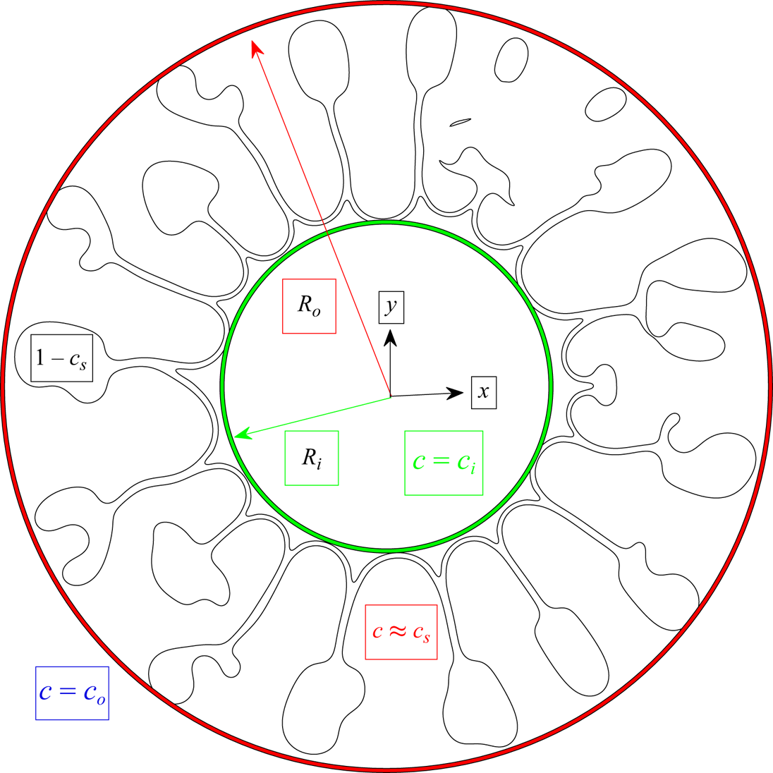
We consider a Hele-Shaw cell of a constant gap thickness  $b$ containing two partially miscible fluids as shown in figure 1. The phase variable c, equivalent to mass fraction in the present model, is designed to have $c = 1$ and $c = 0$ for the fluid viscosity $\eta _1$ and $\eta _2$, respectively, and set that $\eta _{2} > \eta _{1}$. The miscibility of the binary components is $c=c_s$, so the complementary miscibility is $c=1-c_s$. A less viscous mixture of these two components, referred to as the injected fluid thereinafter, with composition $c=c_i$ is injected at the origin ( $x=0$ and $y=0$) to displace a more viscous outer mixture of $c=c_o$, referred to as the displaced fluid. The VF is triggered because of the unfavourable viscosity contrast of the injected and displaced fluid, in which $R_o$ and $R_i$ represent the radius of the circumscribed and the inscribed circle of injected fluid, respectively. Phase separation may occur depending on the local mixture concentration and the interfacial free energy. To simulate the fluid interface, the well-tested Hele-Shaw–Cahn–Hilliard model (Lowengrub & Truskinovsky Reference Lowengrub and Truskinovsky1998; Chen et al. Reference Chen, Huang and Miranda2011, Reference Chen, Huang and Miranda2014; Huang & Chen Reference Huang and Chen2015; Tsuzuki et al. Reference Tsuzuki, Li, Nagatsu and Chen2019b; Li et al. Reference Li, Cai, Chen and Meiburg2022, Reference Li, Lin, Cai, Chen and Meiburg2023; Chou et al. Reference Chou, Huang and Chen2023) is applied. The governing equations for a diffuse-interface approach can be written as
 $$\begin{gather} \boldsymbol{\nabla} \boldsymbol{\cdot} \boldsymbol{u} = 0, \end{gather}$$
 $$\begin{gather}\boldsymbol{\nabla} p ={-}\frac{12\eta }{ {b}^ 2 } \boldsymbol{u} - \epsilon \rho \boldsymbol{\nabla} \boldsymbol{\cdot} ( (\boldsymbol{\nabla} c) \times (\boldsymbol{\nabla} c)^{\rm T}), \end{gather}$$
 $$\begin{gather}\rho \left(\frac{\partial c}{\partial t} + \boldsymbol{u} \boldsymbol{\cdot} \boldsymbol{\nabla} c\right) = \alpha {{\nabla}}^2 \mu . \end{gather}$$
Here,  $\boldsymbol {u}$, $p$,
$p$,  $\rho$ and $\eta$ denote the velocity vector, the pressure, the density and the viscosity, respectively. Here $\epsilon$ and $\alpha$, respectively, represent the coefficient of capillary and mobility. Here $\mu$ stands for the chemical potential of the phases. It is noticed that the effect of density difference on the VF can be ignored, which is concluded in Suzuki et al. (Reference Suzuki, Nagatsu, Mishra and Ban2020) so that it is also assumed negligible on the phase separation. As a result, constant density is taken in the model.
Principal sketch of the simulation set-up. A less viscous binary-fluid mixture with concentration  $c$ of $c=c_i$ is injected at the origin ( $x=0$ and $y=0$) to displace a more viscous outer fluid of $c=c_o$. The miscibility of the binary fluids is $c=c_s$. Here $R_o$ and $R_i$ represent the radius of the circumscribed and the inscribed circle of injected fluid, respectively. Because of partial miscibility, the areas inside and between the fingers are mixing zones where the concentration can reach $c\approx 1-c_s$ and $c\approx c_s$, respectively.
In this diffuse-interface framework, the viscosity of fluid mixture ( $\eta$) is assumed to be related to $c$ with an exponential contrast constant $R_v$ as (Chen & Meiburg Reference Chen and Meiburg1998a,Reference Chen and Meiburgb; Petitjeans et al. Reference Petitjeans, Chen, Meiburg and Maxworthy1999)
 \begin{equation} \eta(c) = \eta_1 \exp({[R_v(1-c)]}), \quad R_v=\ln \left ( \frac{\eta_2}{\eta_1} \right ). \end{equation}
In a stable injection, i.e.  $\eta _{1} \geqslant \eta _{2}$, we assume at a characteristic time $t_c$, the area of the injected fluid would expand circularly to a characteristic radius of $R_c$. By this, the injecting strength $Q$ can be written as ${Q}={\rm \pi} ({R_c}^2-{R_0}^2)/ t_c$, where $R_0$ is the radius of injecting hole. Driven by the injection, the interface becomes unstable in the present unfavourable viscosity contrast, resulting in complex interfacial shapes as time progresses.
The expression of the phase potential  $\mu$ and the profile of Helmholtz free energy $f_0$ for a partially miscible interface is proposed as
 $$\begin{gather} \mu = \frac{\partial f_0}{\partial c} - {\epsilon } {{\nabla}}^2 c, \end{gather}$$
 $$\begin{gather}f_0 = (c-c_{s1})^2 (c-c_{s2})^2 f^*, \end{gather}$$
where  $f^*$ is a characteristic energy. The case which satisfies $c_{s1}=0$, $c_{s2}=1$, $c_i=1$ and $c_o=0$ corresponds to the fully immiscible condition successfully applied in Chen et al. (Reference Chen, Huang and Miranda2011, Reference Chen, Huang and Miranda2014) and Tsuzuki et al. (Reference Tsuzuki, Li, Nagatsu and Chen2019b). In the recent simulations of gravity-driven CO $_2$ flows of low solubility, an asymmetric profile of $c_{s1}=0.05$ and $c_{s2}=1$ is adapted (Li et al. Reference Li, Cai, Chen and Meiburg2022, Reference Li, Lin, Cai, Chen and Meiburg2023). A relatively simple symmetric profile of $c_{s1}=c_s$ (miscibility) and $c_{s2}=1-c_s$ (complementary miscibility) is used to prescribe the partial miscible conditions in the present study. It has been ensured that the qualitative patterns and the responsible mechanisms are consistent even if an asymmetric profile is applied. The dimensionless profiles of
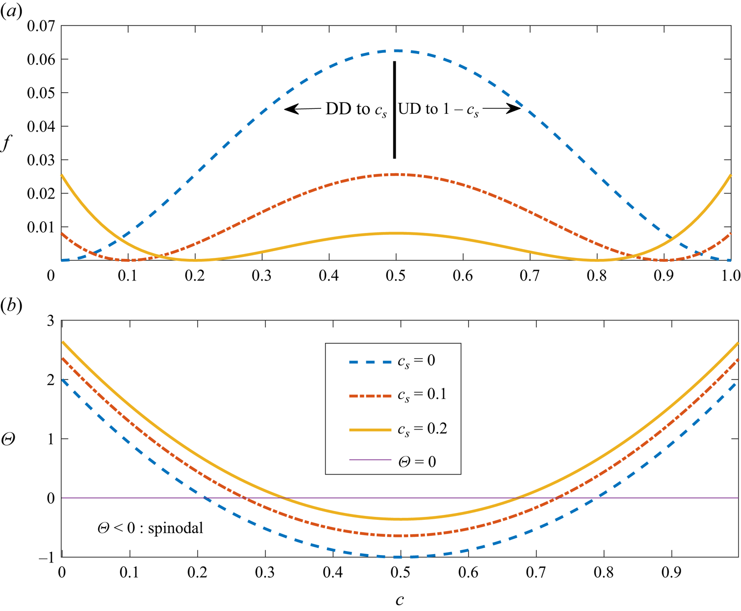
  $f=f_0/f^*$ for various $c_s$ are shown in figure 2. According to the value of $\varTheta$, defined as $\varTheta \equiv {\partial ^2 f}/{\partial c^2} =12(c^2-c+\frac {1}{6})+4(c_s-c_s^2)$, the binary fluid mixture possesses distinct physical features (Shinozaki & Oono Reference Shinozaki and Oono1992; Suzuki et al. Reference Suzuki, Nagatsu, Mishra and Ban2020; Kim et al. Reference Kim, Palodhi, Hong and Mishra2023). A thermodynamically unstable region, denoted as the spinodal region, exists if $\varTheta < 0$, e.g. $0.269< c<0.731$ for $c_s=0.1$, as shown in figure 2. The mixture undergoes phase separation (or spinodal decomposition) within the spinodal region. Outside of the spinodal region and bounded by the miscibility $c_s$ and complementary miscibility $1-c_s$ where $f$ is minimum, the fluid mixture is metastable, e.g. $0.731< c<0.9$ and $0.1< c<0.269$ for $c_s=0.1$. Under the metastable condition, the fluid remains stable unless the external disturbance is sufficiently strong.
(a) Profiles of free energy  $f$ of various miscibility $c_s$, and (b) their correspondent magnitude of second derivative $\varTheta \equiv {\partial ^2 f}/{\partial c^2}$. Uphill diffusion (UD) and downhill diffusion (DD) proceed towards complementary miscibility $1-c_s$ and miscibility $c_s$, respectively. Spinodal decomposition occurs when $\varTheta < 0$.
In order to make the governing equations and relevant variables dimensionless,  $2R_c$, $t_c$ and $\epsilon$ are taken as the characteristic scales. Furthermore, the pressure and the free energy are scaled by $(48 \eta _1 R_{c}^{2}) / (b^2 t_c)$ and the characteristic specific energy $f^*$, respectively. Thus, the dimensionless versions of the governing equations become
 $$\begin{gather} \boldsymbol{\nabla} \boldsymbol{\cdot} \boldsymbol{u} = 0, \end{gather}$$
 $$\begin{gather}\boldsymbol{\nabla} p ={-} {\eta} \boldsymbol{u} - \frac{ C }{I} \boldsymbol{\nabla} \boldsymbol{\cdot} \left [ (\boldsymbol{\nabla} c) \times (\boldsymbol{\nabla} c)^{\rm T} \right ], \end{gather}$$
 $$\begin{gather}\frac{\partial c}{\partial t} +\boldsymbol{u} \boldsymbol{\cdot} \boldsymbol{\nabla} c = \frac{1}{{ Pe}} {{\nabla}}^2 \mu, \end{gather}$$
associated with the following dimensionless correlations:
 $$\begin{gather} \eta = \exp({[R_v(1-c)]}), \end{gather}$$
 $$\begin{gather}\mu = \frac{\partial f}{\partial c} - C {{\nabla}}^2 c. \end{gather}$$
 The dimensionless parameters, such as the Péclet number  ${Pe}$, the logarithm viscosity contrast $R_v$, the Cahn number $C$ and the injection parameter $I$, are defined as
 \begin{equation} {Pe}=\frac{4\rho R^2_c}{\alpha f^* t_c}, \quad R_v= \ln \left(\frac{\eta_2}{\eta_1}\right), \quad C=\frac{\epsilon}{ 4R^2_c {f}^*}, \quad I=\frac{48 \eta_1 R^2_c }{\rho b^2 f^* t_c }. \end{equation}
The Péclet number ( $Pe$) and the Cahn number ( $C$) are the dimensionless measures of dissipation and dispersion in the model (Lowengrub & Truskinovsky Reference Lowengrub and Truskinovsky1998).
2.2. Numerical methods
The numerical methods we employ in this work are similar to the ones developed in Chen et al. (Reference Chen, Huang and Miranda2011, Reference Chen, Huang and Miranda2014), Huang & Chen (Reference Huang and Chen2015) and Li et al. (Reference Li, Cai, Chen and Meiburg2022), in which the continuity and momentum equations are reformulated into the well-known stream function–vorticity ( $\psi$– $\omega$) system as
 $$\begin{gather} u =\frac{\partial \psi}{\partial y},\quad v ={-}\frac{\partial \psi}{\partial x}, \end{gather}$$
 $$\begin{gather}\omega = \boldsymbol{\nabla} \times \boldsymbol{u}, \end{gather}$$
 $$\begin{gather}{{\nabla}^2} \psi ={-} \omega, \end{gather}$$
 $$\begin{gather}\omega ={-} {R_v} \left ( u\frac{\partial c}{\partial y}-v\frac{\partial c}{\partial x} \right ) + \frac{C}{ \eta I } \left[ \frac{\partial c}{\partial x} \left ( \frac{\partial^3 c}{\partial x^2 \partial y} +\frac{\partial^3 c}{\partial y^3} \right ) -\frac{\partial c} {\partial y} \left ( \frac{\partial^3 c}{\partial x \partial y^2} + \frac{\partial^3 c}{\partial x^3} \right )\right ]. \end{gather}$$
 The total velocity  $\boldsymbol {u}$ is decomposed into two parts, i.e. the rotational and potential parts. The rotational part of the velocity is obtained numerically by solving the stream function equation. On the other hand, the potential part of radial velocity ( $\boldsymbol {u}_{pot}$) induced by injection, which involves singularity at the origin, is smoothed out by distributing its strength in a Gaussian way over the circular core region, i.e. $r \leqslant R_0$. The magnitude of the dimensionless potential radial velocity that satisfies the requirements can be expressed as (Chen et al. Reference Chen, Huang and Miranda2014; Huang & Chen Reference Huang and Chen2015; Chou et al. Reference Chou, Huang and Chen2023)
 \begin{equation} \boldsymbol{u}_{pot} = \frac{Q}{2{\rm \pi} r} [1-\exp{({-}4r^2 / {R_0}^2)}]\boldsymbol{r}, \end{equation}
where  $\boldsymbol {r}$ represents the unit vector along the radial direction. The dimensionless injection strength $Q$, which is fixed, takes the form as
 \begin{equation} {Q}= \frac{{\rm \pi} (1-4{R_0}^2)}{4}. \end{equation}
 The simulations are performed in a square computational domain with a length of 2, i.e.  $(x,y) \in [-1,1] \times [-1,1]$. An initially circular injecting core, whose radius is set at $R_0=0.08$, is placed at the centre of the domain with $c=c_i$, while the area outside the core is $c=c_o$. The initial interfacial region between $c_i$ and $c_o$ is smoothly connected by an error function type profile (Chen & Meiburg Reference Chen and Meiburg1998a). The boundary conditions of the system are prescribed as follows:
 $$\begin{gather} x ={\pm} 1\ :\ \psi = 0, \quad \frac{\partial c}{\partial x}=0,\quad \frac{{\partial}^2 c}{\partial x^2}=0, \end{gather}$$
 $$\begin{gather}y ={\pm} 1\ :\ \psi= 0, \quad \frac{\partial c}{\partial y}=0,\quad \frac{{\partial}^2 c}{\partial y^2}=0. \end{gather}$$
The complete set of governing equations, i.e. the concentration  $c$, the vorticity $\omega$ and stream function $\psi$, are numerically solved by a highly accurate compact finite difference discretization associated with pseudospectral method (Chen et al. Reference Chen, Huang and Miranda2011, Reference Chen, Huang and Miranda2014; Huang & Chen Reference Huang and Chen2015; Li et al. Reference Li, Cai, Chen and Meiburg2022). Time integration for the concentration $c$ is fully explicit and utilizes a third-order Runge–Kutta procedure. Spatial discretizations are performed by compact finite differences of fourth- and sixth-order accuracy for the convective and diffusive terms, respectively. A uniform grid size of $\Delta x=\Delta y= \frac {1}{512}$ is applied. Dynamical time step ( $\Delta t$) determined by the local maximum Courant–Friedrichs–Lewy number (CFL), i.e. ${\rm CFL} = ({\Delta t}/{\Delta x})(u,v)_{max}=0.1$, is applied to advance in time.
The updated concentration  $c$ is discretized by a sixth-order compact finite difference scheme to evaluate the vorticity. Then, the Poisson equation of the stream function is solved by a pseudospectral method, in which a Galerkin-type discretization using a cosine expansion is employed in the $x$-direction and a sixth-order compact finite difference in the
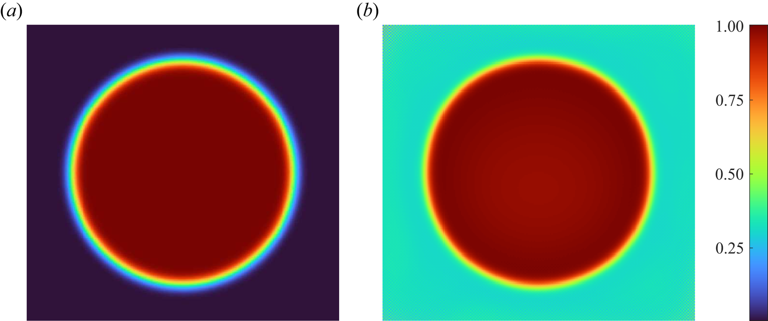
  $y$-direction. Shown in figure 3 is the phase separation of a partially miscible drop for $c_s=0.2$ without external convection. The initial concentration ( $t=0$) of the drop and the surrounding fluid are $c=1$ and $c=0$, respectively. The partial miscibility results in the phase separation, in which the drop concentration and the surrounding fluid gradually approaches $c=0.8$ and $c=0.2$, respectively, as shown at $t=1$. The separation phase agrees with the sketches of figure 1(b) in Suzuki et al. (Reference Suzuki, Nagatsu, Mishra and Ban2020). Additional validations of the present methods are supported by the good qualitative and quantitative agreements with experiments and linear stability analysis achieved in the early works of rotational flows (Chen et al. Reference Chen, Huang and Miranda2011), suction flows (Chen et al. Reference Chen, Huang and Miranda2014) and gravity-driven flows (Li et al. Reference Li, Cai, Chen and Meiburg2022). Similar numerical schemes have also been recently implemented on a reactive condition (Sharma et al. Reference Sharma, Pramanik, Chen and Mishra2019; Tsuzuki et al. Reference Tsuzuki, Li, Nagatsu and Chen2019b). For more details on the implementations of the present numerical methods and their validations in non-reactive and reactive Hele-Shaw flows, the reader is referred to Chen et al. (Reference Chen, Huang and Miranda2011, Reference Chen, Huang and Miranda2014), Huang & Chen (Reference Huang and Chen2015), Li et al. (Reference Li, Cai, Chen and Meiburg2022), Tsuzuki et al. (Reference Tsuzuki, Li, Nagatsu and Chen2019b) and Sharma et al. (Reference Sharma, Pramanik, Chen and Mishra2019), respectively.
Phase separation of a partially miscible drop for  $c_s=0.2$ at (a) $t=0$ and (b) $t=1$.
3. Results and discussion
It is noticed that phase separation occurs when the system is thermodynamically unstable, for instance, in the spinodal region. On the other hand, VF is triggered when the interface of the two fluids becomes hydrodynamically unstable, such as the displacement of one more viscous fluid by another less viscous fluid. Even though the causes of these two interfacial phenomena are distinct by their underlying mechanisms, the continuous process of morphological change by phase separation and VF is both called unstable or interfacial instability in the following presentation for easier understanding. The main objective is to study VF and phase separation coupling effects. Hence, the concentration of injected fluid  $c_i$ is within the $0.5\leqslant c_i<1-c_s$ range to trigger possible phase separation. The study primarily focuses on the influences of concentration of the injected fluid $c_i$ and the miscibility $c_s$. In the following presentation, the rest of the parameters are fixed as $R_v=3.5$, $Pe=50$, $C=10^{-5}$, $I=12.5$, and $c_o=0$ unless mentioned.
3.1. Pattern formation
Shown in figure 4 are the concentration images of three representative cases of a fixed  $c_s=0.1$ for $c_i=0.5$, $c_i=0.6$, and $c_i=0.7$ at $t=0.25$, 0.5, 1.0, 1.5. Based on figure 2, all three cases are in the spinodal region, i.e. $\varTheta <0$, so phase separation of the injected fluid is expected. In addition, because of the magnitude of $\varTheta$, i.e. $| \varTheta (c_i=0.5) | >| \varTheta (c_i=0.6) | >| \varTheta (c_i=0.7) |$, the prominence of phase separation would be in the order of $c_i=0.5$, $c_i=0.6$, $c_i=0.7$. These cases are carried out without initial disturbances, so the patterns appear artificially symmetric. The corresponding randomly perturbed simulations are shown in figure 5 for direct comparison. The symmetric patterns by non-perturbed conditions result in consistent features of the overall patterns, such as droplets or slim-stem fingers, with their correspondent perturbed asymmetric counterparts. Even though the perturbed conditions are more realistic, their highly irregular patterns might hinder the detailed analysis. As a result, the ideally non-perturbed simulations are used for the latter discussion because of their more straightforward pattern formation.
Representative series, images of concentration of  $R_v=3.5$, $Pe=50$, $C=10^{-5}$, $I=12.5$ and $c_s=0.1$ at $t=0.25$, 0.5, 1.0, 1.5. Here (a–d) $c_i=0.5$; (e–h) $c_i=0.6$; (i–l) $c_i=0.7$.

Images of perturbed initial concentration for  $R_v=3.5$, $Pe=50$, $C=10^{-5}$, $I=12.5$ at $t=1.5$. Here (a) $c_s=0.1$ and $c_i=0.5$; (b) $c_s=0.1$ and $c_i=0.6$; (c) $c_s=0.1$ and $c_i=0.7$; (d) $c_s=0$ and $c_i=0.5$.

It is noticed that the number of fingers remains identical regardless of the prominence of phase separation, i.e. the value of  $c_i$. This indicates that the dominant instability at the early time is VF, which triggers the same number of fingers by fixed viscosity contrast and interfacial tension in all three cases. As time proceeds, because the fluids are partially miscible, the concentration of the injected and the displaced fluid tends to separate to the complementary miscibility at $c=0.9$ and the miscibility at $c=0.1$, respectively. For the most thermodynamically unstable case of $c_i=0.5$ shown in figure 4(a–d), several protruding fingers evolve at $t=0.25$. The concentration of these protrusions appears denser, e.g. close to the complementary miscibility $c=0.9$, than the inner circular core area, which is the aftermath of phase separation. In the meantime, apparent mixing to the miscibility $c=0.1$ proceeds outside the core and between fingers. The concurrence of two instabilities, i.e. hydrodynamical VF and thermodynamical phase separation, is observed and forms an interesting corona pattern. At $t=0.5$, the denser fingers keep evolving. They are cut off by the thermodynamical phase separation, as shown in figure 4(b), which is hardly observed in conventional hydrodynamic VF. As time proceeds to $t=1.0$, multiple low-concentration (more viscous) grooves and high-concentration (less viscous) ridges develop azimuthally around the boundary of the core and the phase is completely separated to form fluid threads. At
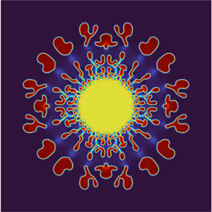
  $t=1.5$, when the simulation is terminated, the overall pattern appears broken with numerous isolated fluid fragments. The formation of droplets (or fluid fragments) is in line with experiments (Suzuki et al. Reference Suzuki, Nagatsu, Mishra and Ban2020, Reference Suzuki, Kobayashi, Nagatsu and Ban2021a).
To further elucidate the phase separation, the concentration profiles between  $0\leqslant x \leqslant 1$ along the centreline ( $\,y=0$) are shown in figure 6(a). Because of phase separation, the concentration profile appears non-monotonically, oscillating between $c_i=0.5$ and $c_o=0$ at $x=0$ and $x=1$, respectively. At $t=0.25$, two oscillating cycles exist. Because of the continuous supply of injected fluid, the amplitude of waves closer to the origin is smaller. The amplitude is much more significant for the second oscillation, whose maximum and minimum concentration reaches nearly the complementary miscibility $c=0.9$ and the miscibility $c=0.1$, respectively. The dramatic drop in concentration from $c=0.9$ to $c=0.1$ corresponds to the formation of isolated fragments or droplets shown in the image. A smooth transition evolves from $c\approx 0.1$ to $c=1$ at the outermost region. As a result, three regions are categorized between injected fluid ( $c_i$) and displaced fluid $(c_o)$, such as (1) the phase separation from $c=c_i$ $(0.5)$ to $c \approx 1-c_s$ $(0.9)$, (2) the sharp interface from $c\approx 1-c_s$ $(0.9)$ to $c \approx c_s$ $(0.1)$ and (3) the diffusive mixing from $c\approx c_s$ $(0.1)$ to $c=c_o$ $(0)$. The peaks and troughs of oscillating waves caused by phase separation correspond to the more dilute grooves and the denser ridges observed around the circular core in figure 4, respectively. In the meantime, the partial miscibility results in a sharp interface bounded by miscibility amid $c_s$ and $1-c_s$. Limited diffusion takes place beyond the miscibility $c_s>c>c_o$. As time proceeds, the continuous phase separation produces more oscillating waves (grooves and ridges). These oscillating waves are also propagated outwardly by the injection flow in the present condition, as shown in figure 6(a). The completeness of the sharp interface and diffusive region is broken by the prominent formation of droplets along the centreline at later times $t\geqslant 0.5$, also shown in figure 6(a).
Concentration profiles along the centreline ( $\,y=0, 0\leqslant x \leqslant 1$) of $c_s=0.1$ at $t=0.25$, 0.5, 1.0 and 1.5: (a) $c_i=0.5$, (b) $c_i=0.6$ and (c) $c_i=0.7$, whose correspondent images are shown in figure 4.

There are two effects for increasing  $c_i$: strengthening the VF because of the lower viscosity of the injected fluid, i.e. $\eta _{injected} = \exp ({(1-c_i)R_v})$, and weakening the phase separation due to lower magnitude of $\varTheta$ as shown in figure 2. Consequently, VF is more dominant over phase separation. Also shown in figures 4 and 6 are the concentration images and concentration profiles, respectively, of higher $c_i=0.6$ (figures 4e–h and 6b) and $c_i=0.7$ (figures 4i–l and 6c). As expected, instead of the formation of broken fluid fragments, the fingers are much better preserved and evolve continuously. Only a few droplets are observed at the fingertips in the cases of $c_i=0.6$. For the case of $c_i=0.7$, VF dominates, so no fingers are completely separated to form droplets. Nevertheless, even though the fingers evolve continuously, their shapes are distinct from the conventional viscous fingers. The denser fingertip appears bulb-shaped with a slim stem connecting the core, developing from corona-shaped at early time to lollipop-shaped later. It is worth mentioning again that the interesting lollipop-shaped patterns resemble what had been observed in the experiments (Suzuki et al. Reference Suzuki, Tada, Hirano, Ban, Mishra, Takeda and Nagatsu2021b). The weakening phase separation results in less significant oscillation of the concentration profiles. The three regions described above, such as phase separation, sharp interface and diffusive mixing, are preserved for the concentration profiles along the centreline. Notably, the interesting lollipop-shaped pattern is anomalous in Newtonian fluids but involves a significant thermodynamic effect. Bulbed fingertips are observed if the viscosity variation between the injected and displaced fluid is non-monotonic with a minimum in the interfacial area, for instance, the fingering pattern obtained in reactive flows in which the least viscous species is produced by a chemical reaction between the injected and displaced fluid (Sharma et al. Reference Sharma, Pramanik, Chen and Mishra2019). Nevertheless, slim and elongated finger stems do not form. Despite the uniqueness, thermodynamic effects have only been considered very recently. The mechanisms that generate such unique lollipop-shaped fingers and droplets will be explained in more detail later in this section.
A few unique features of the overall pattern are worthy of further discussion. The pattern mainly consists of four parts: (i) inner core  $c=c_i$, (ii) mixing zone $c\approx c_s$ and (iii) fluid fragments (droplets) or fingers $c\approx 1-c_s$, which correspond to the regions indicated by green, red and black texts, respectively, shown in figure 1. Additionally, (iv) dilute grooves and dense ridges exist between the core (or finger) and mixing zone. To better illustrate these parts, the representative concentration profile associated with droplets of $c_i=0.5$ and $c_s=0.1$ at $t=1.5$ is shown in figure 7. The concentration remains $c=0.5$ inside the inner core as the region marked by the letter $c$. Subsequently, the profile starts to oscillate, in which the troughs and peaks represent the low-concentration grooves (marked by the letter $g$) and high-concentration ridges (marked by the letter $r$), respectively. Nevertheless, the concentration of troughs/peaks is significantly higher/lower than the miscibility $0.1/0.9$, which indicates the pattern is not fully separated to form isolated fluid fragments of droplets. The mixing zones, marked by the letter $m$, are the nearly flat regions where concentrations remain close to the miscibility, i.e. $c\approx 0.1$. Between the mixing zones, where concentration drops from $c \approx 0.9$ to $c\approx 0.1$, are the isolated fluid fragments or droplets marked by the letter $d$.
$d$.
Enlarged view of concentration profiles between  $0.25 \leqslant x \leqslant 0.8$ along the centreline ( $\,y=0$) of $c_s=0.1$, and $c_i=0.5$ at $t=1.5$. The letters $c$,
$c$,  $g$,
$g$,  $r$,
$r$,  $d$ and $m$ represent the core, groove, ridge, droplet and mixing area, respectively.

The mechanisms of these parts can be understood by the close view of another representative concentration profile of  $c_i=0.6$ and $c_s=0.1$ at $t=1.5$ shown in figure 8 and is also elucidated in figure 9. As mentioned above, the profile can be divided into three regions: (1) the phase separation from $c=0.6$ to $c \approx 0.9$, (2) the sharp interface from $c\approx 0.9$ to $c \approx 0.1$ and (3) the diffusive mixing from $c\approx 0.1$ to $c=0$. It is worth noting that, in the present milder condition, the region of phase separation can be further distinguished into two subregions of the spinodal instability and metastable region from $c=0.6$ to $c=0.731$ and $c=0.731$ to $c \approx 0.9$, respectively. As shown in figure 8, areas of concentration higher than the injected fluid, i.e. the denser ridge of $c > 0.6$, exist in the spinodal region. Hence, the expansion of the inner core to the ridge is viscously stable and remains nearly circular. On the other hand, the outer front of the densest concentration of the sharp interface, whose viscosity is the smallest, can further enhance hydrodynamical fingering instability to the displaced fluid. If the local strength of phase separation is sufficiently strong, the protruding fingers may be separated, forming isolated fragments or droplets. Finally, the injected and displaced fluid can partially mix because of finite miscibility. Zones of limited mixing with a maximum concentration of $c_s=0.1$ are located beyond the sharp interface, which corresponds to the diffusive region presented in figure 8. Another interesting observation is the transition of concentration profile from the spinodal region to the metastable region. Unlike non-monotonic oscillating waves of concentration in the spinodal region, as shown in figure 8, the concentration profile monotonically increases within the meta-stable range, i.e. from $c=0.731$ to the complementary miscibility of $c=0.9$. The different behaviours verify the two distinct modes of thermodynamical instability in the spinodal and metastable regions.
Enlarged view of concentration profiles between  $0.3 \leqslant x \leqslant 0.9$ along the centreline ( $\,y=0$) of $c_s=0.1$, and $c_i=0.6$ at $t=1.5$.

Sample sketch for the elucidation of the interfacial phenomena. Radial concentration distribution evolves from the core to the diffusive region, e.g. along the purple arrow as the representative profile shown in figure 8. The UD and DD, taking place towards the radial (blue arrow) and azimuthal (red arrow) orientations, result in slim-stem fingers.

It should be pointed out that the lollipop pattern, which is not observed in the hydrodynamical VF instability, is primarily related to thermodynamic instability, i.e. the competition between metastable states and spinodal decomposition. In the present source flow configuration, the radial distance of the injected fluid can also represent the evolving time for thermodynamic instability, i.e.  $r \sim \sqrt {t}$. Therefore, the ripening time increases from the core centre towards the fingertips. As demonstrated in figure 8, the concentration profile is divided into three regions depending on the distance from the centre, i.e. the nearest core, the middle spinodal region and the farthest metastable region. Consequently, the metastable region has the longest ripening time, while the spinodal decomposition zone has an intermediate ripening time. The core, where the concentration is the same as the injected fluid, has a very short ripening time. Suppose the injected fluid is in a spinodal state, which is the present condition; the spontaneous separation results in concentration oscillation, in which the local concentration can be higher and lower than the injected fluid, as shown in figure 8. The portion separated into higher concentrations will undergo diffusion towards the high equilibrium concentration (the complementary miscibility $1-c_s$), referred to as the UD. In contrast, the portion of the fluid separated into lower concentrations will undergo diffusion towards the low equilibrium concentration (the miscibility $c_s$), referred to as the DD. The orientations of the UD and DD are demonstrated in figures 2 and 9.
If the highest/lowest amplitude of the oscillating concentration profile, induced by spinodal decomposition, reaches  $1-c_s$/ $c_s$ within the repining time, respectively, the fluids are completely separated to form droplets. Otherwise, the concentration of UD proceeds radially so that regions of high concentration (low viscosity) continuously evolve away from the core and eventually far enough to pass the state of spinodal decomposition. Subsequently, it becomes metastable, where phase separation is no longer significant. The concentration increases monotonically by the UD towards the complementary miscibility and then drops to the miscibility, forming a sharp interface as also shown in figure 8. On the other hand, the DD proceeds circumferentially towards the outer fluid of the low-concentration region. Local concentration gradually decreases and eventually reaches the miscibility, mixing with the outer fluid. The DD along the azimuthal direction continuously decreases the local concentration to thinning the middle portion, i.e. the finger's stem. On the contrary, the radially UD results in high concentrations at the fingertip. Driven by the radially injected flow, the thinning stem is elongated. In the meantime, the least viscous fingertip swells to form a lollipop-shaped pattern. Sufficient ripening time of the metastable state allows these unique features to evolve, forming the lollipop-shaped pattern.
In summary, under sufficiently large  $\varTheta$ conditions in which spinodal separation is dominant, as shown in figure 7, the concentration oscillates dramatically without an apparent region of smooth growth towards the maximum. So that no distinguishable metastable state is observed. Once the amplitude reaches the miscibility and complemental miscibility, the continuous concentration supply by the UD is cut off so that isolated fragments or droplets evolve. On the other hand, a lollipop-shaped finger forms when the spinodal region (concentration oscillation) and metastable state (monotonic growth of concentration) coexist.
3.2. Parametric study
The miscibility  $c_s$ is another crucial parameter to determine the magnitude of $\varTheta$ as shown in figure 2. Based on figure 2, a lower $c_s$ for a fixed $c_i$ results in a higher magnitude of $\varTheta$; thus, more prominent phase separation is expected. In the meantime, a lower $c_s$ increases the concentration drop (or viscosity contrast) on the sharp interface, i.e. from $c=1-c_s$ to $c=c_s$ as shown in figure 8 to trigger more vigorous fingering locally. The patterns for a lower $c_s=0$ with various $c_i=0.5$, 0.6 and 0.7 are shown in figure 10. These three conditions are all within the spinodal region. The pattern is highly broken for the most vital phase separation of $c_i=0.5$ and $c_s=0$, as shown in figure 10(a–d). The typical structures caused by phase separation, such as numerous isolated fragments around the core, multiple layers of droplets, and multiple circularly dilute grooves and dense ridges, are more prominent. These main features of the pattern are also preserved in the perturbed condition, as shown in figure 5(d). Another interesting observation is that the core size does not change significantly. It is the aftermath of the continuous formation of the circular grooves and ridges by phase separation. Under the present condition, the ability of the injecting source can no longer effectively suppress the phase separation to push away the continuous formation of the circular grooves and ridges from the origin. The continuous evolvements of circular grooves/ridges and fragments associated with the apparent growth of cutoff fingers indicate that the phase separation and the VF remain prominent throughout the injection process. All the above phenomena can also be observed in the concentration profiles shown in figure 11(a). The number and amplitudes of waves are much higher, which reflects the more prominent phase separation. Because of $c_s=c_o$, no diffusive zone exists with the concentration drop amid the sharp interface from $c\approx 1$ to $c \approx 0$. The onset location of the wave, which can be approximated as the radius of the core, remains nearly unchanged. A more quantitative analysis of the core size will be discussed in a later section.
Images of concentration of  $R_v=3.5$, $Pe=50$, $C=10^{-5}$, $I=12.5$ and $c_s=0$ at $t=0.25$, 0.5, 1.0, 1.5. Here (a–d) $c_i=0.5$; (e–h) $c_i=0.6$; (i–l) $c_i=0.7$.

Concentration profiles along the centreline ( $\,y=0$, $0\leqslant x\leqslant 1$) of $c_s=0$ at $t=0.25$, 0.5, 1.0 and 1.5: (a) $c_i=0.5$, (b) $c_i=0.6$ and (c) $c_i=0.7$, whose correspondent images are shown in figure 10.

Cases of higher  $c_i=0.6$ and 0.7 are also shown in figure 10(e–h) and figure 10(i–l). As mentioned in the previous section, the prominence of phase separation is weakened, so the number of fragments from the isolated grooves/ridges and droplets by the cutoff fingers is reduced for $c_i=0.6$. The injected fluid is completely unbroken for the case of $c_i=0.7$. In addition, the size of the core gradually increases. For the case of the weakest phase separation $c_i=0.7$, the increase of the core size is the most apparent. These reflect the fewer number and farther onset locations of the waves of concentration profiles at various times, as shown in figures 11(b) and 11(c). In the meantime, strengthening the VF results in tip-split at the tips of lollipop-shaped fingers.
The influence of miscibility can be realized by comparing the three series of  $c_s=0.1$, $c_s=0$ and $c_s=0.2$ shown in figures 4, 10 and 12, respectively. Note that the case of $c_s=0.2$ and $c_i=0.7$ shown in figure 12(e–h) is in the metastable region. Unlike the effects of $c_i$, a decrease of $c_s$ strengthens both the phase separation because of a larger magnitude of $\varTheta$, and VF due to a higher viscosity contrast at the sharp interface, i.e. $\Delta \eta _{interface} = \exp ({(1-c_s) R_v}) - \exp ({c_s R_v})$ as shown in figures 6 and 11. As a result, among the cases presented, the pattern appears the most fragmented for the case of $c_s=0$ and $c_i=0.5$ featuring multiple layers of isolated fragments and droplets along the circular core and fingers, respectively, as shown in figure 10(a–d). On the other hand, the effect of phase separation is the weakest for the case of $c_s=0.2$ and $c_i=0.7$, in which no droplets are formed as shown in figure 12(e–h). It is interesting to compare the patterns of the case of $c_s=0.1$ and $c_i=0.6$ shown in figure 4(e–h) with the case of $c_s=0$ and $c_i=0.7$ shown in figure 10(i–l), whose magnitudes of $\varTheta$ are identical, i.e. $\varTheta =-0.52$. For the case of $c_s=0$ and $c_i=0.7$ whose $\Delta \eta _{interface}$ is higher, fingering appears more vigorous, e.g. longer length of fingers with splits at the tips. Nevertheless, the main features of phase separation of these two cases remain similar, such as barely formed droplets and lollipop-shaped fingers. The similarity between these two cases suggests that the magnitudes of $\varTheta$ dominate the phase separation.
Images of concentration of  $R_v=3.5$, $Pe=50$, $C=10^{-5}$, $I=12.5$ and $c_s=0.2$ at $t=0.25$, 0.5, 1.0, 1.5. Here (a–d) $c_i=0.5$; (e–h) $c_i=0.7$.
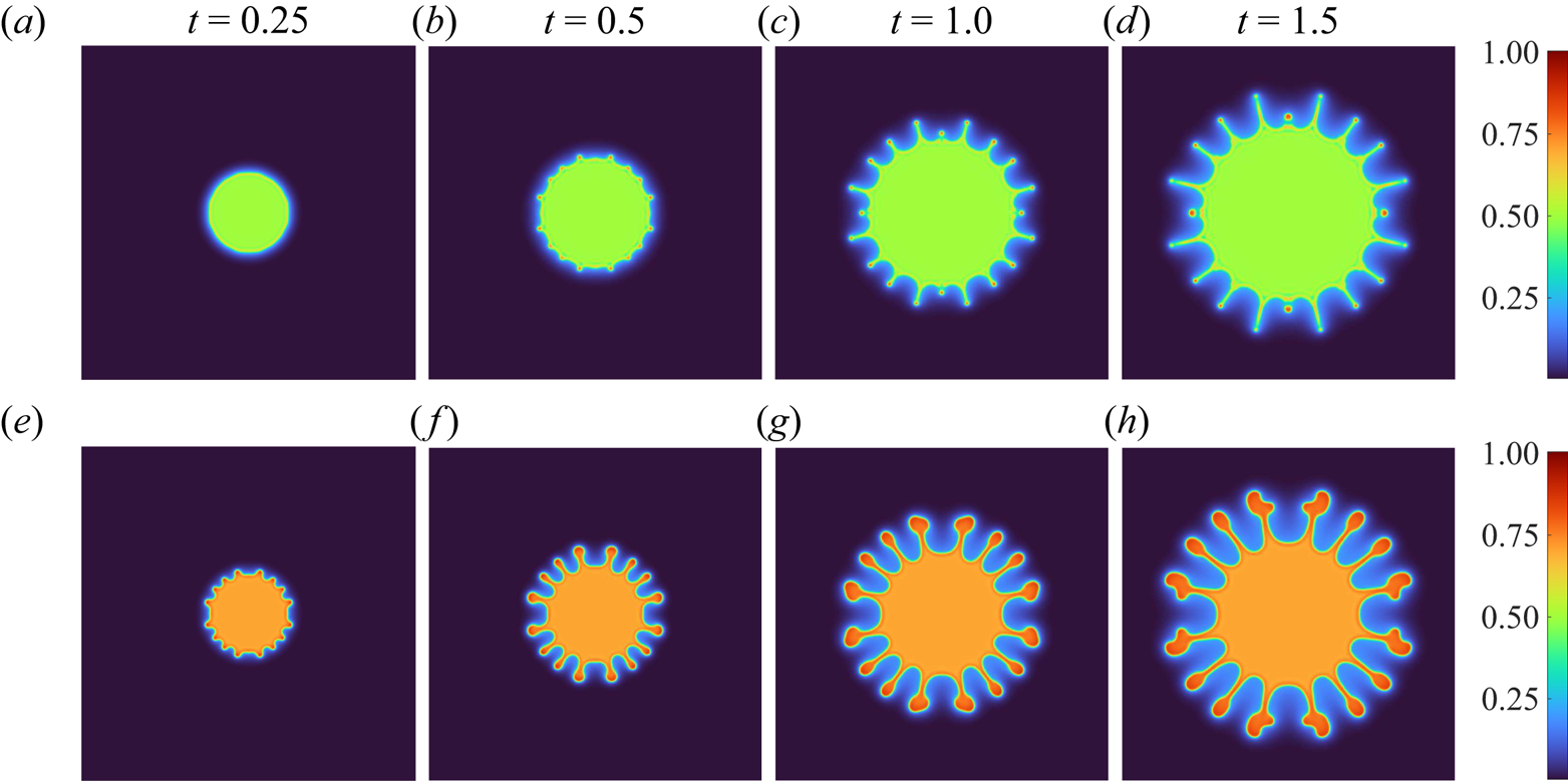
To complete the study, all the rest of the parameters, such as the viscosity contrast  $R_v$, the mobility $Pe$, the Cahn number $C$, and the injection parameter $I$, are varied to evaluate their influences as the images at $t=1.5$ shown in figure 13. The reference values of parameters are for $R_v=3.5$, $C=10^{-5}$, $I=12.5$, $c_s=0$, $c_i=0.6$. Only the studied parameter varies for each group, while others are fixed, such that the influence of $c_i$, $C$,
$C$,  $c_s$, $R_v$, $Pe$ and $I$ is demonstrated in figures 13(a,b), 13(b,c), 13(b,d), 13(a,e), 13(b, f) and 13(c,g), respectively.
Influences of various parameters: (a,b)  $c_i=0.5$ and $c_i=0.6$; (b,c) $C=10^{-5}$ and $C=5\times 10^{-6}$; (b,d) $c_s=0.1$ and $c_s=0$; (a,e) $R_v=3.5$ and $R_v=2.3$; (b, f) $Pe=50$ and $Pe=25$; (c,g) $I=12.5$ and ${I=6.25}$; (d,h) $Pe=50$ and $Pe=200$.

Figures 13(a) and 13(e) are the cases for  $R_v=3.5$ and $R_v=2.3$, respectively, in a condition of strong phase separation ( $c_s=0.1$ and $c_i=0.5$). Not too much fingering instability is triggered for the case of $R_v=2.3$ as expected, so the pattern appears as numerous fragments and droplets without preferable orientation. On the contrary, for the case of $R_v=3.5$, even though no continuous fingers are observed, fingering instability can be distinguished by the radial alignments of droplets along several cutoff fingers.
The prominence of phase separation, as presented in the previous sections, is mainly determined by the magnitude of  $\varTheta$, which is the second derivative of dimensionless free energy $\varTheta \equiv ({1}/{f^*})({\partial ^2 f_0}/{\partial c^2})$. Because the characteristic free energy $f^*$ appears in the denominator of dimensionless expression of $Pe$,
$Pe$,  $C$ and $I$, these parameters may also play a role in the influence of phase separation. Consequently, a more prominent effect of phase separation may be expected for lower $Pe$,
$Pe$,  $C$ and $I$, i.e. larger $f^*$. Figures 13(b) and 13( f) are the cases for $Pe=50$ and $Pe=25$, respectively, in a condition of milder phase separation ( $c_s=0.1$ and $c_i=0.6$). The phase separation for $Pe=25$, compared with $Pe=50$, is significantly strengthened by forming continuous threads and reducing the size of the circular core. In contrast, the cases of $Pe=50$ and $Pe=200$ in a condition of $c_s=0$ and $c_i=0.6$, as shown in figures 13(d) and 13(h), a higher $Pe=200$ completely prevents the formation of broken fragments and droplets, indicating weaker phase separation. Nevertheless, the fingering instability is slightly enhanced for $Pe=200$ with the more apparent tip-split, consistent with the common expectation of conventional VF. The results indicate the strong influence of $Pe$ on the pattern formation, especially the effect of phase separation. Besides the reason for the scaling factor $f^*$, this is also understood by the fundamental mechanism of the concentration equation, in which $Pe$ explicitly controls the response of phase separation.
The Cahn number  $C$ and the injection parameter $I$ are also related to the effective interfacial tension (Chen et al. Reference Chen, Huang and Miranda2011, Reference Chen, Huang and Miranda2014; Tsuzuki et al. Reference Tsuzuki, Li, Nagatsu and Chen2019b). A weaker interfacial tension (lower $C$ and larger $I$) results in a more unstable interface. The influence of $C$ can be observed by comparing the cases of $C=10^{-5}$ and $C= 5 \times 10^{-6}$ shown in figures 13(b) and 13(c), respectively. The pattern of lower $C= 5 \times 10^{-6}$, compared with $C=10^{-5}$, appears more unstable for phase separation with broken fragments around the core and droplets along the fingers. In the meantime, VF is also more vigorous, with tip-split at the fingertips. As a result, $C$ can also affect the overall pattern significantly. On the other hand, even though a lower $I$ could enhance the phase separation, it may be offset by a stronger effect of interfacial tension. As shown in figures 13(c) and 13(g) for $I=12.5$ and $I=6.25$, respectively, the overall patterns remain similar with only minor differences.
3.3. Pattern categorization and quantitative analysis
To summarize the patterns presented above, four types can be quantitatively categorized such as (i) CS, (ii) FS, (iii) SF and (iv) LF, whose particular interfacial patterns and rotational streamlines are shown in figures 14 and 15, respectively. To more clearly demonstrate the patterns, interfaces at  $t=1.5$ shown in figure 14 are represented by the values of $\tau (x,y)$ defined as
 \begin{equation} \tau(x,y) = \left(\frac{\partial c}{\partial x}\right)^2 + \left(\frac{\partial c}{\partial y}\right)^2. \end{equation}
Note that  $\tau (x,y)$ is also related to the magnitudes of local interfacial tension (Chen et al. Reference Chen, Huang and Miranda2011, Reference Chen, Huang and Miranda2014; Tsuzuki et al. Reference Tsuzuki, Li, Nagatsu and Chen2019b). Nevertheless, unlike the immiscible situation, in which a simple sharp interface exists between the injected and displaced fluids, the entire interfacial area in the present partially miscible condition includes a sharp-drop interface and prolonged diffusive area, as shown in figure 8. As a result, the conventional treatment of surface tension may not be suitable and not discussed here.
The four typical types of interfacial patterns, represented by the contours of  $\tau$. (a) Core separation (CS) for $R_v=2.3$, $Pe=50$, $C=10^{-5}$, $c_s=0.1$ and $c_i=0.5$. (b) Fingering separation (FS) for $R_v=3.5$, $Pe=50$, $C=10^{-5}$, $c_s=0$ and $c_i=0.5$. (c) Separation fingering (SF) for $R_v=3.5$, $Pe=50$, $C=5 \times 10^{-6}$, $c_s=0.1$ and $c_i=0.6$. (d) Lollipop fingering (LF) for $R_v=3.5$, $Pe=200$, $C=10^{-5}$, $c_s=0$ and $c_i=0.6$.

Streamlines of the four typical patterns shown in figure 14: (a) CS; (b) FS; (c) SF; (d) LF.

For the case dominated by prominent phase separation ( $c_s=0.1$ and $c_i=0.5$) associated with milder VF ( $R_v=2.3$) as shown in figure 14(a), the interfaces feature multiple layers of tiny fragments distributed around the circular core without preferred orientations. The overall pattern appears wholly broken. The typical vortex pairs commonly seen in the conventional VF (Chen & Meiburg Reference Chen and Meiburg1998a; Tsuzuki et al. Reference Tsuzuki, Li, Nagatsu and Chen2019b) are insignificant, as shown in figure 15(a). Since the separated fluid fragments mainly form around the core without apparent fingers, thus this pattern is called core separation. If both the influences of phase separation and VF are strengthened, e.g. $c_s=0$ and $R_v=3.5$ as shown in figures 14(b) and 15(b), even though the interface remains almost completely broken, apparently outward expansion of multilayer droplets can be distinguished, indicating the vigorous fingering. On the other hand, the isolated fragments around the core develop reversely inward because of strong separation. The streamlines consist of multilayer vortex pairs, the typical structures of fingering instability, but significantly scattering without concentrating flow paths. The pattern is categorized as FS because its viscous fingers are entirely cut off, breaking the overall pattern by phase separation.
The previous two patterns possess the typical features of phase separation, i.e. fluid fragments and droplets. On the other hand, fingering formation can be better preserved if the prominence of phase separation is weakened, e.g.  $c_i=0.6$ and $c_s=0.1$ for $R_v=3.5$, as shown in figures 14(c) and 15(c). The formation of viscous fingers is well retained; even droplets form at the tips. The cutoff fingers result in a two-layer formation of vortex pairs in the streamlines. In addition, flow paths of denser streamlines connecting the two layers of vortex pairs indicate the better development of viscous fingers. This pattern is called SF because distinguishable fingers are preserved with fewer droplets. Finally, if the influence of phase separation is further reduced by taking a higher $Pe=200$ as patterns shown in figures 14(d) and 15(d), the cutoff of injected fluid is completely suppressed. Nevertheless, as discussed in the previous section, the fingers appear lollipop-shaped with slim stems and bulb tips. As a result, the streamlines consist of continuous flow paths connected with the wide vortex pairs at the tips. This unconventional fingering pattern is categorized as LF.
To quantify the pattern, the radius of the circumscribed  $(R_o$) and the inscribed circle $(R_i)$ of injected fluid, as marked in figure 1, is measured by the outermost and the innermost position of $c_i$, respectively. The mixing radius $R_m$ representing the longest length of fingers is defined as $R_m=R_o-R_i$. It is worth mentioning that $R_i$, representing the initial position of the concentration oscillation, can be viewed as the onset of phase separation. Hence, a shorter $R_i$ corresponds to a more prominent phase separation. Shown in figure 16(a) are $R_i$ and $R_m$ of the three cases presented in figure 10, representing the three conditions of vigorous fingering as FS $(c_i=0.5)$, SF $(c_i=0.6)$ and LF $(c_i=0.7)$. Note that fingering is not significant for the case of CS and is not measured. For the condition of FS $(c_i=0.5)$, $R_i$ does not keep increasing, or even decreasing, at later times even though the injection continues. The decrease of $R_i$ confirms the prominent phase separation of the dilute grooves and dense ridges around the core and is the unique feature to categorize the dominance of phase separation. On the contrary, for the conditions of SF $(c_i=0.6)$ and LF $(c_i=0.7)$, $R_i$ increases with time due to the injection of fluid, which behaves similarly to conventional VF. Nevertheless, the continuous increase of $R_m$ for all three conditions indicates the active growth of fingers. The $R_m$ is in the opposite trend with $R_i$, in which the $R_m$ is longer for stronger phase separation. $R_o$, i.e. $R_o=R_i+R_m$, remains nearly the same for all three cases due to the same viscosity contrast at the fingering interface between the injected fluid and displaced fluid, i.e. identical $c_s$. So, an increased $R_m$ for more prominent phase separation mainly decreases the core size $R_i$. At the same time, the position of outwardly evolving fingers $R_o$ is determined by VF. As shown in figure 16(a), the shorter $R_i$ and longer $R_m$ of FS deviate apparently from the other two cases of SF and LF in which the VF dominates.


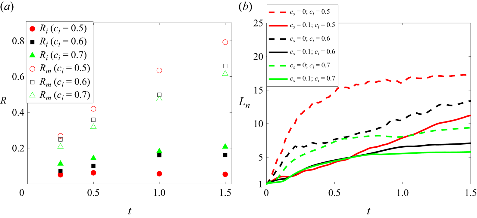
Another measure used to quantify the instability is the interfacial length  $L(t)$, which can be approximated by (Chen & Meiburg Reference Chen and Meiburg1998a)
 \begin{equation} L(t) = \int_x \int_y \sqrt{\tau(x,y)} \,{\rm d}\kern0.07em x\,{\rm d}y. \end{equation}
A normalized length  $L_n$ is scaled by the circumference of a stable injection without phase separation (Tsuzuki et al. Reference Tsuzuki, Li, Nagatsu and Chen2019b; Chou et al. Reference Chou, Huang and Chen2023) and shown in figure 16(b) for the cases whose images are demonstrated in figures 4 and 10. Note that the condition of $L_n=1$ represents a stably circular pattern, so the value of $L_n$ represents the prominence of interfacial instability. The immediate growths of $L_n$ shown in figure 16(b) are due to the prominent phase separation around the core, such as formations of grooves and ridges, so that the initial growth rates at $t=0$ directly depend on the magnitudes of $\varTheta$, i.e. a higher initial growth rate for a larger $\varTheta$. For instance, the initial growth rates of $c_s=0$ and $c_i=0.7$ are very close to $c_s=0.1$ and $c_i=0.6$, whose $\varTheta$ are identical. The temporal development of $L_n$ is strongly affected by the miscibility $c_s$ and the concentration of injected fluid $c_i$. A smaller $c_s$ results in a sharper interface. Besides, a lower $c_i$ leads to a more non-monotonic concentration distribution in the separation region. Consequently, $L_n$ is longer for a smaller $c_s$ or $c_i$. The different temporal evolution of $L_n$ for the distinct patterns can also be observed. $L_n$ of the FS ( $c_s=0$ and $c_i=0.5$) is the largest because of the additional interface caused by rapid phase separation. Nevertheless, the growth of $L_n$ is very insignificant at the later times. On the other hand, in the case of SF, $L_n$ keeps growing even though the $L_n$ is lower than the FS. As shown in figure 16(b), the temporal trends of $L_n$ of the two SF cases, e.g. $c_s=0$ and $c_i=0.6$, $c_s=0.1$ and $c_i=0.5$, are quite similar. Finally, for the three cases of LF ( $c_s=0$ and $c_i=0.7$, $c_s=0.1$ and $c_i=0.6$, $c_s=0.1$ and $c_i=0.7$) shown in figure 16(b), their $L_n$ are the lowest, with gradually diminishing growth rates.
Based on the results discussed above, a pattern diagram is summarized in figure 17, showing the distribution of four categorized patterns, such as the CS, the FS, the SF and the LF. The pattern is mainly determined by the value of  $\varTheta$ if other parameters are fixed. For instance, isolated fragments or droplets are formed if $\varTheta < -0.5$ for a representative series of $R_v=3.5$ $Pe=50$, $C=10^{-5}$ and $I=12.5$. The effect of phase separation is the most significant in the case of $\varTheta =-1$ so that the fingers are completely separated, forming the pattern of FS. As the increase of $\varTheta$, weaker separation results in SF. For the cases of $\varTheta > -0.5$, phase separation is further weakened, so the pattern appears in the LF. The CS occurs if the viscosity contrast is sufficiently low, e.g. $R_v=2.3$. In addition, the pattern may be altered by varying other parameters, for instance, from LF to SF by lowering $Pe$,
$Pe$,  $C$ or $I$.
$I$.
Pattern diagram for CS (Core), FS, SF and LF (Lollipop). The empty marks represent cases of  $R_v=3.5$, $Pe=50$, $C=5\times 10^{-5}$ and $I=12.5$. The colour-filled marks are cases with varied parameters.

3.4. Qualitative comparison with experiments
It is noticed that the present simulations emphasize verifying and analysing the newly observed anomalous pattern in VF. Even direct quantitative comparisons are not presently feasible because of the lack of knowledge of the key parameters, e.g. the exact free energy profile, chemical potential, capillary coefficient and mobility, quantitative comparison with experimental results is crucial to validate the simulations.
A similar trend has also been discovered in experiments. The partially miscible systems have been designed by varying the compositions of sodium sulphate ( ${\rm Na}_2{\rm SO}_4$) and PEG in water (Suzuki et al. Reference Suzuki, Nagatsu, Mishra and Ban2020, Reference Suzuki, Tada, Hirano, Ban, Mishra, Takeda and Nagatsu2021b; Iwasaki et al. Reference Iwasaki, Nagatsu, Ban, Iijima, Mishra and Suzuki2023). The less viscous sodium sulphate solution is injected to displace the more viscous PEG solution as the four typical patterns shown in figure 18. Note that the four cases are all within the region of phase separation (Suzuki et al. Reference Suzuki, Nagatsu, Mishra and Ban2019). Identical conditions of the last three cases are also previously experimented with and reported in Suzuki et al. (Reference Suzuki, Nagatsu, Mishra and Ban2020, Reference Suzuki, Tada, Hirano, Ban, Mishra, Takeda and Nagatsu2021b) and Iwasaki et al. (Reference Iwasaki, Nagatsu, Ban, Iijima, Mishra and Suzuki2023). In these experiments, the viscosity contrast increases slightly from figures 18(a) to 18(d). Particularly, for cases figures 18(b) to 18(d) of identical PEG concentration, the prominence of phase separation gradually weakens as decreasing concentration of ${\rm Na}_2{\rm SO}_4$ (Suzuki et al. Reference Suzuki, Nagatsu, Mishra and Ban2020). Therefore, a quantitative analogy can be made that the magnitude of negative $\varTheta$ also decreases from case figures 18(b) to 18(d).
Experimental images of typical phase separation coupled VF patterns. (a) Core separation, 20 wt % sodium sulphate solution displaces 30 wt % polyethylene glycol (PEG) solution ( $R_v=3.2$); (b) FS, 20 wt % sodium sulphate solution displaces 36.5 wt % PEG solution ( $R_v=4.0$); (c) SF, 17 wt % sodium sulphate solution displaces 36.5 wt % PEG solution ( $R_v=4.2$); (d) LF, 10 wt % sodium sulphate solution displaces 36.5 wt % PEG solution ( $R_v=4.5$). For cases (b)–(d) of identical PEG concentration, the prominence of phase separation gradually weakens as decreasing concentration of ${\rm Na}_2{\rm SO}_4$ (Suzuki et al. Reference Suzuki, Nagatsu, Mishra and Ban2019). Note that (a–c) are within the spinodal region, while (d) is metastable.

For the case in figure 18(a), the viscosity contrast is the smallest, so VF is the least vigorous. Dominated by the strong spinodal decomposition, droplets form around the injected core. If the viscosity contrast is increased, as shown in figure 18(b), VF starts to show visible influence so that apparent fingers evolve simultaneously with droplets. For the case of figure 18(c), with even higher viscosity contrast and weaker spinodal decomposition, VF becomes the dominant mechanism. As a result, the pattern appears in apparent fingers with few detached droplets. Thus, figures 18(a), 18(b) and 18(c) are comparable to the CS, FS and SF, respectively. On the other hand, no detached droplets are observed for the case of the highest viscosity contrast with the weakest effect of phase separation, shown in figure 18(d). Similar to the simulations, several fingers in figure 18(d) featuring slim finger stems with bulb tips correspond to the LF in the simulation. The trend of coupling influence of VF and phase separation in these four experiments is consistent with the cases presented in figure 14 so that the patterns can be qualitatively compared. The good agreement of pattern evolution between the simulations and experiments justifies the present categorization.
Additional comparisons with the simulations can be made by the quantitative measures of core radius  $R_i$, mixing radius $R_m$ and normalized interfacial length $L_n$. These radii are averaged by measuring the lengths of dominant fingers and scaled by the radius of the circular experimental region. Because the experiments are terminated at the breakthrough time, when the outmost finger reaches the boundary, the experimental duration varies among these experiments. The dimensionless time is represented by instantaneous injection volume $V_i$ scaled by the total volume injected in the case of figure 18(d), in which the largest volume $V_o$ is injected. Shown in figure 19 are the cases demonstrated in figures 18(b), 18(c) and 18(d), which correspond to the pattern of FS, SF and LF, respectively. They can be compared with the simulation results of similar patterns shown in figure 16. The evolving trends of $R_i$ and $R_m$, as demonstrated in figure 19(a), also appear consistently with the simulation presented in figure 16(a). Here $R_i$ is the shortest for the case of FS, which corresponds to the strongest phase separation, and increases consequently with the dominance of VF, i.e. SF and LF.
(a) Core radius  $R_i$ and mixing radius $R_m$, and (b) normalized interfacial length $L_n$ for the experiments shown in figures 18(b), 18(c) and 18(d), which corresponds to the pattern of FS, SF and LF, respectively. Qualitatively consistent trends are observed with the simulation results shown in figure 16.

Even though  $L_n$ might seem not completely consistent between figures 19(b) and 16(b), i.e. the solid curves with the same colour in the two figures, it can be rationalized by the viscosity contrast. The viscosity contrast in experiments is the highest in the case of figure 18(d) (i.e. LF) so that rapidly emerging VF increases $L_n$ at a very early time. Nevertheless, the growth rate of $L_n$ remains insignificant as time proceeds because of the lack of droplets. On the other hand, for cases of figure 18(c) (i.e. SF) and figure 18(b) (i.e. FS), even the $L_n$ are much shorter at early time because of less vigorous VF, as time proceeds, formation of droplets caused by prominent phase separation result in rapid growth of $L_n$. As a result, $L_n$ in the FS condition surpasses the LF condition shortly after. It is also anticipated that $L_n$ in the SF condition will exceed the LF condition if the experiment lasts sufficiently long. A consistent trend with simulations is expected, such that $L_n$ is in the order of FS, SF and LF. The qualitative agreements of these measures also justify the correctness of the present simulation.
4. Conclusions
The anomalous fingering patterns reported in experiments, i.e. the tip-widening finger with a slim stem (referred to as the LF) and droplets, which are the aftermath of both thermodynamic (phase separation) and hydrodynamic (i.e. VF) instability, have been numerically verified by the Hele-Shaw–Cahn–Hilliard model incorporating a symmetric double-well free energy profile. By this model, the positions of the lowest free energy (or wells) represent the miscibility and complementary miscibility of the binary fluids. The composition is in an equilibrium state at the miscibility, so phase separation may occur if the local concentration is not equal to the miscibility or the complementary miscibility. The injected fluid is a less viscous binary mixture to trigger VF. In addition, the composition of injected fluid is in the spinodal or metastable region, i.e. the concentration amid the miscibility and the complementary miscibility, to induce phase separation. Because of VF, phase separation and partial miscibility, the concentration distribution between the injected fluid and displaced fluid mainly includes four parts: the inner core; the grooves and ridges; the isolated fragments or droplets; the mixing zone, respectively located from the origin of injection source outwardly. Similar to the conventional VF, the concentration within the circular core remains at the concentration of injected fluid. Subsequently, phase separation occurs in the spinodal and metastable regions, where the concentration is bounded by injected concentration and miscibility, forming low-concentration grooves and high-concentration ridges around the core. If the separation is sufficiently strong, such that the grooves and ridges reach nearly the miscibility and complementary miscibility, the fluids are completed separated, forming broken fragments. If the vital phase separation happens inside viscous fingers, the fingers are cut off, forming droplets. This dramatic separation featuring a non-monotonic concentration profile of grooves, ridges or broken fragments is mainly formed in the spinodal region. In contrast, the concentration monotonically approaches complementary miscibility in the metastable region. On the other hand, the displaced fluid also partially mixes to approach the miscibility, forming a mixing zone. As a result, a sharp interface exists between the metastable region and mixing zone, whose concentration drops nearly from the complementary miscibility to miscibility. The non-monotonic concentration profile, containing both spinodal and metastable regions, results in lollipop-shaped fingers, referred to as LF, distinct from the conventional viscous finger, whose monotonic concentration profile evolves radially outward.
By coupling VF with phase separation, four typical types of patterns are categorized: CS; FS; SF; LF, in the order of the dominance of phase separation. For the patterns of CS and FS, isolated fluid fragments or droplets around the inner core is the main feature so that the inner core radius does not continuously increase or may decrease at later times as injection proceeds. Consequently, the interfacial length deviates dramatically from the stably circular shape. If the VF is not vigorous, like in the case of lower viscosity contrast, the isolated fragments have no apparent aligned orientation. The pattern is categorized as CS. On the other hand, if the VF is also vigorous, in addition to the isolated fragments around the core, droplets along distinguished cutoff fingers also form. This pattern is categorized as FS since the fingers are entirely cut off by phase separation. If the effect of phase separation is weakened, the development of isolated fragments around the core is less prominent. The formation of fingers is better preserved and thus categorized as SF. As a result, the core's radius and the pattern's interfacial length increase as injection proceeds. In the case of weakest phase separation, the formation of isolated fluid fragments and droplets is entirely suppressed. Nevertheless, phase separation still results in a non-monotonic concentration profile; the shape of the fingers is lollipop-shaped, consisting of a slim stem connecting the circular core and bulb tips. Therefore, this pattern is called LF. These patterns are in line with experiments of partially miscible sodium sulphate and PEG solutions.
Finally, a pattern diagram mainly focusing on the magnitude of the second derivative of the free energy profile is summarized. The influence of the rest of the dimensionless parameters, such as the viscosity contrast, the mobility, the Cahn number and the injection parameter, on the four patterns is also presented by parametric simulations.
Funding
We thank Taiwan's National Center for High-performance Computing (NCHC) of National Applied Research Laboratories (NARLabs) for providing computational and storage resources. C.-Y.C. acknowledges the financial support from the R.O.C. (Taiwan) National Science and Technology Council through the project NSTC 111-2221-E-A49-087-MY3. Financial support of JSPS KAKENHI grant nos 22K3900 and 22K20402, and JST PRESTO grant no. JPMJPR22O5 is also acknowledged. The authors thank Dr P. Verma and Mr J. Mao for their assistance in analysing additional data in revision.
Declaration of interests
The authors report no conflict of interest.


 Open access