Geographical setting

Hurd Peninsula ice cap (62˚39–42'S, 60˚19–250W; Fig. 1), Livingston Island, South Shetland Islands, Antarctica, covers an area of about 10 km². The main ice cap is drained by several outlet glaciers: Argentina, flowing northwestwards; Las Palmas, flowing westwards; Sally Rocks tongue, flowing southwestwards; an unnamed tongue flowing southwards (which we refer to as MacGregor glacier); and Johnsons Glacier, flowing northwestwards, which is additionally fed by ice draining not from the main ice cap but from the east and northeast. For the latter reason, Hurd Peninsula ice cap is often subdivided into two main glacier units: Johnsons Glacier, a tidewater glacier; and Hurd Glacier, the remaining ice mass, mostly terminating on land. The local ice divide separating Johnsons and Hurd has altitudes of 250– 330ma.s.l. The main body of Hurd Glacier has an average surface slope of ~3˚, though its westward-flowing side lobes, Argentina and Las Palmas, have much steeper slopes (~13˚). These are even higher in MacGregor glacier, which is entirely a heavily crevassed icefall. Typical slopes for Johnsons Glacier range between 10˚ in its northern areas and 6⁸ in the southern areas.

Fig. 1. Location of Livingston Island and Hurd Peninsula, and surface map of Johnsons and Hurd Glaciers showing the contour lines of the digital terrain model for 1999–2000. Contour interval is 5 m.

Background

Previous glaciological studies of Hurd Peninsula ice cap have been made with the logistic support of the Spanish Antarctic station Juan Carlos I (JCI), close to Johnsons Glacier (see Fig. 2), and most of them therefore focus on Johnsons Glacier. These studies include mass balance and ice dynamics from stake measurements and shallow–intermediate ice cores (Reference Furdada, Pourche and VilaplanaFurdada and others, 1999; Reference XimenisXimenis and others, 1999; Reference Vasilenko, Sokolo, Machere, Glazovsk, Cuadrad and NavarroXimenis, 2001), geomorphology (Reference Ximenis, Calve, Enriqu, Corber, Fernández de Gambo and FurdadaXimenis and others, 2000), numerical modelling of ice dynamics (Reference Martín, Navarr, Oter, Cuadrad and CorcueraMartín and others, 2004; Reference OteroOtero, 2008), ice-volume changes from aerial photographs and ground-based surface topography (Reference Molina, Navarro, Calver, García-Sellés and LapazaranMolina and others, 2007), and seismic and radar studies (Reference Benjumea, Machere, Navarr and TeixidóBenjumea and others, 2003; Reference Navarro, Machere and BenjumeaNavarro and others, 2005) which we detail later. These studies have shown that the ice surface velocities of Johnsons Glacier increase downstream from the ice divide, reaching values up to 44ma^–1 near the calving front, while the largest ice velocities for Hurd Glacier are typically about 4ma^–1. Accumulation and ablation rates show a large spatial and temporal (yearly) variability, with maximum accumulation rates of about 1 mw.e. a^–1 and maximum ablation rates up to –4mw.e. a^–1 measured over the last 10 years. The equilibrium-line altitude of Johnsons Glacier is ~150m and 180–260m on its northern and southern parts respectively, while that for Hurd Glacier is 250–270m and ~200m on its northern and southern parts, respectively. From the thermal point of view, Hurd Peninsula ice cap has traditionally been considered as temperate, on the basis of limited temperature–depth profiles measured at some shallow–intermediate boreholes (Reference Furdada, Pourche and VilaplanaFurdada and others, 1999), which have been claimed as consistent with measurements at other locations in the South Shetland Islands (e.g. Reference Orheim and GovorukhaOrheim and Govorukha, 1982; Reference Qin, Zielinsk, German, Re, Wan and WangQin and others, 1994), and also on the basis of measured radio-wave velocities in ice (Reference Benjumea, Machere, Navarr and TeixidóBenjumea and others, 2003). We show later that this assumption of a wholly temperate thermal regime should be reviewed.

Fig. 2. Radar profiles (20–25 MHz, and also 200 MHz for accumulation area) covering Johnsons and Hurd Glaciers. Most of them correspond to surveys of December 1999, 2000 and 2001. The locations of the low-frequency CMP measurements are shown as large dots numbered 1–10, while those for low-frequency radar are shown as small dots labelled R1, R3, R4. The small dots labelled BH1, BH2 and BH3 correspond to the locations of the intermediate-depth boreholes drilled in 1999/2000 by M. Pourchet and J.M. Casas (personal communication, 1999). The line joining A–B– C corresponds to the radar section shown in Figure 5. The star denotes the location of Juan Carlos I station.

Previous radar measurements

JCI station operates only during the austral summer season. Within this period, December presents the best snow conditions for radio-echo sounding. Several radar campaigns were carried out between December 1999 and December 2004, using both low (20–25 MHz)- and high (200 MHz)-frequency impulse radars, providing full coverage of Hurd and Johnsons Glaciers, except for the highly crevassed terminus area of the latter and MacGregor icefall (Fig. 2). The details are given in the methods section. Such radar data have been used for multiple purposes: defining the glacier geometry for numerical modelling experiments (Reference Martín, Navarr, Oter, Cuadrad and CorcueraMartín and others, 2004; Reference OteroOtero, 2008), estimating the water content from radio-wave velocities retrieved from diffraction hyperbolae recorded during radar profiling (Reference Benjumea, Machere, Navarr and TeixidóBenjumea and others, 2003), intercomparing the capabilities of radar and seismic methods for the study of glaciers (Reference Navarro, Machere and BenjumeaNavarro and others, 2005) and estimating the total volume of ice stored by Hurd Peninsula ice cap (Reference Molina, Navarro, Calver, García-Sellés and LapazaranMolina and others, 2007).

Aims of current study

In addition to radar profiling, ten common-midpoint (CMP) measurements with low-frequency radar were carried out in December 2003 in order to determine the column-averaged radio-wave velocity (RWV) in ice and the inferred water content. Similar measurements were performed with high-frequency radar at three locations in the accumulation area in order to determine the average RWV of the firn layer. The details are given in the methods section. These results are so far unpublished, except for some preliminary RWV data retrieved from low-frequency measurements and restricted to four sites on Hurd Glacier (Reference LapazaranLapazaran, 2004). In this paper, we briefly review the earlier radar studies, focusing on low-frequency data, and present and discuss the new data, including CMP measurements and their corresponding estimates for RWV and water content, and their implications in terms of hydrothermal regime and ice dynamics. This is of interest because Johnsons and Hurd Glaciers can be considered representative of many small glaciers in the South Shetland Islands, of both tidewater and land-based margin types, respectively.

Radar profiling and data processing

The radar profiling of Johnsons and Hurd Glaciers was done during several austral summer campaigns, and using different ice-penetrating radars, as detailed in Table 1. The distribution of radar profiles is shown in Figure 2. Low-frequency radars (20–25 MHz) were used for penetration down to the bed, while high-frequency radar (200 MHz) was used for sampling the firn layer. For profiling, transmitter and receiver were placed on separate wood sledges towed by a snowmobile. Recording was made, using common-offset geometry, at a 1 s time interval between records, keeping a constant speed of about 3 ms^–1 or, alternatively, a record for each odometer wheel rotation, the latter implying a distance between adjacent records of 1.55 m. The transmitting– receiving antennae were arranged collinearly, following the profiling direction, with the exception of the December 1999 campaign, in which a parallel arrangement was used to reduce the distance between transmitter and receiver. This was due to antennae size and requirements of the transmitter–receiver synchronization, which was accomplished by a dedicated radio channel in the 1999 campaign, but otherwise used optical cable link. In addition to the radar data, navigation information from both global positioning system (GPS) receiver (operating in stand-alone mode) and odometer was also recorded. For use as control information, the coordinates of all profile end-points (occasionally, some intermediate points) were measured by differential GPS (DGPS).

Table 1. Radar surveys done on Hurd Peninsula and radars employed. The details of VIRL2/VIRL2A and VIRL6 radars can be found in Vasilenko and others (2002) and Reference Berirkashvili, Vasilenk, Machere and SokolovBerirkashvili and others (2006), respectively

The processing of radar data included d.c. correction, amplitude scaling, bandpass filtering, deconvolution and migration. The conversion to depth was done using our best estimate for the RWV, determined by CMP measurements discussed below.

Radio-wave velocity measurements and water-content estimates

Using VIRL-6 radar, CMP measurements were performed in December 2003 at ten locations shown in Figure 2, in order to determine the RWV in ice. At each CMP location, radar pulses were generated in steps of 10 m (5m on either side of the CMP) up to a total distance of about 500m (250m per side), i.e. more than twice the maximum ice thickness in these glaciers (~200 m). The RWV was computed using a single-layer model, but took into account a correction for the surface geometry, which was measured by DGPS. The latter feature is relevant, as it can imply noticeable changes in the estimated RWV as compared to a flat surface model, as is shown by the results.

CMP measurements were also performed in December 2003 using Ramac/GPR (ground-penetrating radar) with 200MHz antennae at three locations in the accumulation area (see Fig. 2), in order to determine the average RWV of the firn layer. At each location, measurements were made in steps of 2 m (1m on either side) up to a total length of 50 m (25m per side). In this case, given the small length of the profiles, a flat surface model was applied.

The water content W in temperate ice can be estimated using the two-component dielectric mixture formulae by Reference LooyengaLooyenga (1965), which, assuming a fully water-saturated mixture (i.e. no ice in the pore space), gives

(1)

where ɛ _i and ɛ _w are the relative dielectric permittivities of solid ice and water, and v _s and c = 300 mμs^–1 are the radio-wave velocities in soaked glacier ice and air, respectively. For the computations, we used ɛ _i = 3.19 and ɛ _w = 86 at the melting point (Reference Macheret and A.F. GlazovskyMacheret and Glazovsky, 2000). Note that the estimates of Wso obtained are only valid for v _s < 168m ms^–1; higher values of v _s are associated either with dry glacier ice or with dry or wet firn, which have densities lower than that of solid ice (917 kgm^–3) (Reference Macheret, Moskalevsk and E.V. VasilenkoMacheret and others, 1993).

An alternative for the computation of the water content in temperate ice is Paren’s mixture formula (Reference ParenParen, 1970), which, again under the assumption of fully water-saturated mixture, gives

(2)

which is known to give water-content estimates lower than those produced by Looyenga’s formula (e.g. Reference LapazaranLapazaran, 2004, ch. 4 and app. A).

Ice-thickness map and basal topography, and estimation of total volume in 2000

The basal topography for Johnsons and Hurd Glaciers was constructed by subtracting the ice thickness, retrieved from radar data for 1999–2001, from the surface topography available from DGPS and total station measurements in 1999/2000 (Reference Molina, Navarro, Calver, García-Sellés and LapazaranMolina and others, 2007). Contour lines of non-glaciated areas were taken from the Servicio Geográfico del Ejército 1 : 25 000 map for Hurd Peninsula (SGE, 1991). The ice volume for 2000 was estimated, using Surfer software, from the ice-thickness map. In order to solve some uncertainties in thickness data from 1999 to 2001 (e.g. zones with bedrock reflection not clearly visible in the radargrams), ice-thickness data from 2003/04 were occasionally used, corrected for mass-balance changes. For the highly crevassed area near Johnsons front, where radar profiling was not possible, the ice volume was estimated by subtracting, from the available surface topography, the bed topography determined by interpolating data from neighbouring areas located further up-glacier (covered by radio-echo sounding) and bathymetric measurements in Johnsons Dock, the bay where Johnsons tidewater glacier discharges (D. García-Sellés, unpublished data).

Radio-wave velocities in ice and firn, and water content in temperate ice

The radargram for a sample CMP (number 10 in Fig. 2) appears in Figure 3, with the straight lines for the direct wave through the air, the refracted wave through the ice surface, as well as the curve for the reflections from the bedrock, clearly seen. Some reflections from internal layers are also evident.

The RWV estimates for the full ice column from bed to surface, and the corresponding depth for the CMP, determined from CMP measurements with low-frequency VIRL-6 radar, are shown in Table 2. For purposes of comparison, velocities computed with both non-flat and flat surface models are included. The corresponding water content in temperate-ice estimates, determined by Looyenga’s and Paren’s formulae, under the assumption of fully water-saturated mixture, is also shown.

Table 2. Column-averaged RWV in ice determined from CMP measurements with 20 MHz radar VIRL-6 at the locations shown in Figure 2. v _s is the RWV of soaked ice, Z is the ice thickness at the CMP, and W _L and W _P are the water contents (expressed as %) determined using Reference LooyengaLooyenga’s (1965) and Reference ParenParen’s (1970) formulae, respectively. Values for CMPs 5 and 7 are not included because they produced too large residuals in the error estimates. Water-content values for velocities above 168 mμs^–1 are not shown because they are meaningless using Equations (1) and (2)

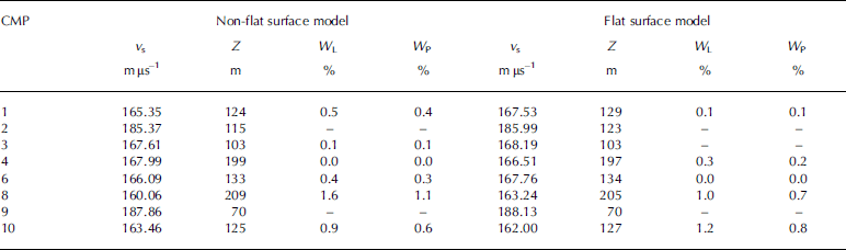
Fig. 3. Radargram for CMP measurement done with VIRL-6 20 MHz frequency radar at the location labelled 10 in Figure 2. The vertical axis shows the two-way travel time (TWT) in ns, while the horizontal axis shows the distance between transmitter (Tx) and Receiver (Rx) in m. W1, W2 and W3 denote, respectively, the direct wave through the air, the refracted wave through the ice surface and the reflected wave from bedrock.

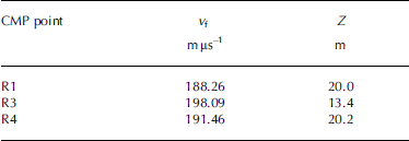
Table 3 presents the results for the RWV estimates for the firn layer, and the depth of the firn–ice interface, determined from CMP measurements with high-frequency Ramac/GPR.

Table 3. Column-averaged RWV in the firn layer determined from CMP measurements with 200 MHz Ramac/GPR at the locations shown in Figure 2

Ice-thickness and subglacial relief maps, and total ice volume

The ice-thickness map constructed from low-frequency radar data is shown in Figure 4a, and the basal topography obtained by subtracting the ice thickness from the surface topography is presented in Figure 4b. The average thickness in 1999–2001 was 93.6 m, with each individual thickness measurement having an estimated error of ±2.5 m. The maximum values, about 200 m, are found in the accumulation area of Hurd Glacier; maximum ice thickness in Johnsons Glacier is only about 160 m. The ice volume estimated from the ice-thickness map, together with the area and average ice thickness for Johnsons and Hurd Glaciers in 1999–2001, are given in Table 4.

Table 4. Area, average ice thickness and ice volume of Johnsons and Hurd Glaciers in 1999–2001. The errors quoted for the average ice thickness do not correspond to the standard deviation of the thickness values but to the vertical resolution of radar data

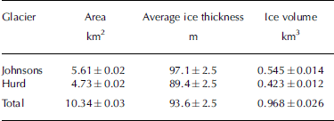
Fig. 4. (a) Ice-thickness map retrieved from the radar measurements; and (b) subglacial relief map obtained by subtracting the ice thickness from the surface topography map. Contour interval is 20 m.

Radio-wave velocity and water content in temperate ice

In Reference Benjumea, Machere, Navarr and TeixidóBenjumea and others (2003), RWVs for Johnsons and Hurd Glaciers were estimated from 42 diffraction hyperbolae corresponding to diffracting bodies between 28 and 162 m depth. The corresponding velocities ranged from 157 to 174mμs^–1, with an average of 164.9±4.2mμs^–1. These are usual values for temperate glaciers (Reference Macheret, Moskalevsk and E.V. VasilenkoMacheret and others, 1993), except those above 168 mμs^–1, which mostly correspond to accumulation area locations and can therefore be attributed to the effect of the snow and firn layers. The corresponding water contents, computed using Equation (1) (Reference LooyengaLooyenga, 1965), were within 0.4–2.3%, with an average of 1.2±0.6%. It is well known, however, that the velocity estimates from CMP measurements are much more accurate than those obtained from diffraction hyperbolae. Essentially, this is because of the uncertainty of the real location of the diffracting bodies, which are assumed to lie in the vertical plane of the radar profile, while actually they are often located off-track. Additionally, CMP velocities provide average values for the full ice–firn column from bed to surface, while diffraction hyperbolae give that from the diffractor to the surface, so that the latter give greater weight to the upper layers, which manifests as a bias towards higher velocities in the accumulation area when they are directly compared with those from CMP measurements.

A look at the RWVs from CMP measurements shown in Table 2 makes evident two main facts:

• 1. The use of a non-flat surface model (i.e. one correcting for the surface undulations) yields results noticeably different from those retrieved using a flat surface model. Differences up to 3 mμs^–1 in RWV, 0.6% in water content and 5 m in ice thickness are shown. Though, at first glance, these may seem not too large, it should be noticed that a shift of 3 mμs^–1 in RWV is as large as that between a typical value for temperate ice (165mμs^–1) and a typical value for cold ice (168mμs^–1). On the other hand, a shift of 0.6% in water content implies, by virtue of Reference DuvalDuval’s (1977) relation between the rate factor in Glen’s flow law and the water content of temperate ice, a change of the effective strain rate by a factor of 2.

• 2. Equation (1) (Reference LooyengaLooyenga, 1965) systematically produces larger water-content estimates than those obtained using Equation (2) (Reference ParenParen, 1970), a fact already pointed out by several authors (e.g. Reference MooreMoore and others, 1999; Reference LapazaranLapazaran, 2004, ch. 4 and app. A). The greatest difference in the table is 0.5%, which corresponds to the non-flat surface model for CMP 8. It should be remembered that Equations (1) and (2) are only strictly valid under the assumption that all pore space between ice crystals is full of water, i.e. no air is present. More proper, though sometimes unfeasible, uses of dielectric mixture formulae for estimating water content in temperate ice are discussed by Reference LapazaranLapazaran (2004).

Two RWV values in Table 2 are unusually high: those for CMPs 2 and 9. The latter can be explained because it corresponds to a location at the accumulation area for which the ice thickness is rather small, 70 m, of which ~20m belongs to the firn layer, thus implying a high velocity. The most likely explanation for the large value at CMP 2 would be the presence of air within the water drainage system.

As regards the RWV for the firn layer, the three 200 MHz CMP measurements reported in Table 3 give consistent results: those for R1 and R3 correspond to the same firn layer thickness and are very similar to each other. Moreover, they average 189.9mμs^–1, which is virtually identical to the value of 190mμs^–1 that is obtained if we apply the relationship between RWV and ice density by Reference Macheret and A.F. GlazovskyMacheret and Glazovsky (2000) to the density data retrieved from the ice core at borehole BH1 (Fig. 2), next to R1 and R3 and not far from R4 (density data courtesy of M. Pourchet and J.M. Casas). It is also consistent with values obtained at other accumulation area locations of similar altitude range within the South Shetland Islands (e.g. 190mμs^–1 in the accumulation area of King George ice cap as reported by Reference Travassos and SimõesTravassos and Simo˜es (2004) from CMP measurements with a pulseEKKO IV 50MHz radar). The RWV given for R3 is not directly comparable to the other values, because it corresponds to the firn above a reflector located at only 12.9m depth, while the firn thickness in this area is about 20m (Reference Furdada, Pourche and VilaplanaFurdada and others, 1999).

Subglacial relief and ice dynamics

Johnsons and Hurd Glaciers are quite different in terms of subglacial relief. Johnsons’ bed is quite regular, with altitudes decreasing towards the ice front, where glacier bed elevation is slightly below sea level. Hurd is more irregular, showing a clear overdeepening in the area of thickest ice, close to the head of Argentina side lobe, and another one, though less pronounced, near the head of Las Palmas side lobe. A promontory is also apparent close to this area, in a line joining the head of Las Palmas and MacGregor Peaks. Two subglacial ridges are visible: one separating Johnsons and Hurd basins (though displaced towards Johnsons with respect to the Johnsons–Hurd ice-divide location) and another extending from Reina Sofia Mount to Sally Rocks, passing through the heads of Argentina and Las Palmas side lobes. All of these features can have an impact on the basal processes and consequently on ice dynamics. It is known that Johnsons and Hurd Glaciers have experienced significant retreat at least from the mid-20th century, with an estimated loss in ice volume of 10.0±4.5% during 1956–2000, equivalent to an average annual balance of –0.23±0.10ma^–1w.e. and consistent with the 1˚C increase in regional summer temperature during this period (Reference Molina, Navarro, Calver, García-Sellés and LapazaranMolina and others, 2007). Johnsons Glacier has shown almost no change in area, but shows a noticeable reduction in volume (7.3%), due to strong ice-thickness decrease. Hurd has experienced an even larger reduction in volume (13.3%), due to its large decrease in area, in spite of having a smaller reduction in ice thickness. It has been shown by these authors that the mass loss for Johnsons is achieved through a combination of increased calving rate and increased melting, while that of Hurd is achieved entirely by increased melting rates, stronger at the lowest elevations, implying increased slopes and hence increased driving stresses. The much larger velocities of Johnsons as compared to Hurd (maximum horizontal velocities of 44 vs 4ma^–1) imply a faster dynamic response of Johnsons Glacier, which tends to restore a steady-state surface profile at a faster rate as compared to Hurd Glacier. Apart from their evident differences as tidewater and land-based glaciers, the differences in subglacial relief and water-content distribution could also play an important role in explaining the different dynamic behaviour of Johnsons and Hurd Glaciers.

In order to understand such a likely contribution, more detailed studies of water-content distribution are needed, to be complemented by modelling experiments presently under way.

Fig. 5. Radar section corresponding to a longitudinal profile of Hurd Glacier, from the ice divide to the terminus (locations A and C in Fig. 2). The vertical arrow marks the position of the equilibrium line. This figure is a composite of a 25 MHz profile (right largest section of figure; location shown in Fig. 2, from A to B) and a 200MHz profile (left smallest section of figure; location shown in Fig. 2, from B to C); the latter does not reach bedrock in part of the profile. In the image of the full profile, the position of the volcanic ash layers is observable in the left of the image, and can be clearly observed in the zoomed image. Their outcrop at the ice surface can be seen in the photographs, which are each taken from the hill shown in the other photograph.

Hydrothermal structure

A final feature that deserves attention in the light of the radar results is the hydrothermal structure of these glaciers. Traditionally, it has been considered that Hurd Peninsula glaciers are temperate (e.g. Reference Furdada, Pourche and VilaplanaFurdada and others, 1999; Reference Vasilenko, Sokolo, Machere, Glazovsk, Cuadrad and NavarroXimenis, 2001; Reference Benjumea, Machere, Navarr and TeixidóBenjumea and others, 2003). This has been justified on the basis of limited temperature–depth profiles measured at some shallow–intermediate boreholes (Reference Furdada, Pourche and VilaplanaFurdada and others, 1999), which have been claimed as consistent with measurements at other locations in the South Shetland Islands (e.g. Reference Orheim and GovorukhaOrheim and Govorukha, 1982; Reference Qin, Zielinsk, German, Re, Wan and WangQin and others, 1994), and also on the basis of average radio-wave velocities in ice determined from diffraction hyperbolae (Reference Benjumea, Machere, Navarr and TeixidóBenjumea and others, 2003). However, we have shown the existence of higher RWVs, typical of cold ice, at least at certain locations. On the other hand, Reference Orheim and GovorukhaOrheim and Govorukha (1982) and Reference Qin, Zielinsk, German, Re, Wan and WangQin and others (1994) suggested that the ice under the accumulation area of the ice caps they studied is temperate, as indeed seems to be the case under the accumulation area of Hurd Peninsula ice cap and other locations in Livingston Island (e.g. Bowles Plateau). However, as can be seen in Figure 5, the radar records show that the ablation area of Hurd Glacier has a surface layer of cold ice, manifested by the area almost free from internal diffractions seen on the left-hand side of the figure, to the left of the arrow indicating the approximate position of the equilibrium line. This cold ice layer has a thickness up to several tens of metres, and reaches bedrock near the glacier snout, implying that ice could be at least partially frozen to bed at this location. This is consistent with having an ice thickness tapering to zero, as insulation is less effective under thinner ice. It is also consistent with the observed velocity field: typical maximum ice velocities for Hurd are only about 4ma^–1 and are reached in the middle to lower part of the glacier, but not near the front of its main tongue. This would be expected for a glacier experiencing some basal sliding in the middle to lower part, but having the glacier snout perhaps frozen to bed. Further evidence supporting our assumption is that geomorphological observations have revealed the presence of structures typical of compressive flow (thrust faults) near Hurd’s snout. Some of these faults are produced along the planes of volcanic ash layer (from eruptions on neighbouring Deception Island) that can be observed in the radar section and the photos in Figure 5. Cold ice patches even appear in some areas under the firn layer in the accumulation zone, but the dominant hydrothermal regime there, as well as at the lower layer in the ablation area, is clearly temperate. Based on radar measurements, cold ice spots have also been suggested to be present near the ice divide of King George Island (Reference Breuer, Lang and BlindowBreuer and others, 2006). Further support for the suggestion of a polythermal regime is given by data assimilation experiments on Hurd Glacier, using a three-dimensional full-Stokes dynamical model (Reference OteroOtero, 2008). These have shown that the value of the stiffness parameter B in Glen’s law (assumed to be constant for the entire glacier) providing the best agreement between observed and computed surface velocities is 0.22 MPa a^1/3, which is quite close to that of 0.20MPa a^1/3 found by Reference HansonHanson (1995) for polythermal Storglacia¨ren, Sweden. The slightly larger values for Hurd Glacier indicate an even colder regime. In light of the above evidence, Hurd Glacier should be considered to be a polythermal glacier, and the assumed temperate thermal regime of other Livingston Island – or, more generally, South Shetland Islands – glaciers should be reviewed.