


1. Introduction
The small-scale intermittency of turbulent flows was first detected decades ago (Batchelor & Townsend Reference Batchelor and Townsend1949), but remains one of the most challenging problems in turbulence theory. In the dissipative scales, the enstrophy (the square of the vorticity vector) and the square of the rate-of-strain tensor concentrate in regions of the flow where they become orders of magnitude more intense than the average, the more so the larger the Reynolds number, apparently without bound (Sreenivasan & Antonia Reference Sreenivasan and Antonia1997; Buaria et al. Reference Buaria, Pumir, Bodenschatz and Yeung2019). These intense events organise in structures of theoretical and practical relevance whose origin and dynamics are not well understood (Jiménez et al. Reference Jiménez, Wray, Saffman and Rogallo1993; Yeung, Zhai & Sreenivasan Reference Yeung, Zhai and Sreenivasan2015; Buaria, Pumir & Bodenschatz Reference Buaria, Pumir and Bodenschatz2020).
A persuasive explanation of the origin of these intense structures comes from models supported by the theory of the energy cascade (Frisch Reference Frisch1995; Biferale Reference Biferale2003). A particularly intuitive and successful class of models consists of those based on multiplicative cascades, which describe intense small-scale events as generated by the successive uneven breakup of eddies through the cascade. This uneven breakup is modelled by the product of multipliers, which leads to the amplification of eddies and to intense events of the dissipation once these eddies reach the dissipative scales. One of the first multiplicative cascade models is due to Kolmogorov (Reference Kolmogorov1962). In order to account for intermittency, he proposed a multiplicative random process for the energy transfer and invoked the central limit theorem to derive a log-normal model of the cascade. Although this model failed to predict the scaling exponents of the structure functions, the idea of a cascade described by the product of multipliers proved fruitful. Frisch, Sulem & Nelkin (Reference Frisch, Sulem and Nelkin1978) proposed a model in which only a fixed fraction of the space is filled by the breakup of eddies, i.e. where some multipliers are zero, leading to a geometry with a single fractal dimension (Mandelbrot Reference Mandelbrot1974). This model, known as the  $\beta$-model, was later generalised to random fractions by Benzi et al. (Reference Benzi, Paladin, Parisi and Vulpiani1984), introducing a much richer geometry, and a non-trivial spectrum of generalised dimensions, or multifractal spectrum (Parisi & Frisch Reference Parisi and Frisch1985; Sreenivasan Reference Sreenivasan1991). This model is not able, however, to reproduce appropriately the manifest part of the multifractal spectrum of the dissipation field (Meneveau & Sreenivasan Reference Meneveau and Sreenivasan1991). Probably the simplest model that accomplishes this is the ${p}$-model by Meneveau & Sreenivasan (Reference Meneveau and Sreenivasan1987), in which eddies break into equal-sized eddies with a fraction $p$ or $1-p$ of the energy flux (in a one-dimensional simplified representation). This simple binomial process describes very well many aspects of the geometry of the dissipation field, and reproduces, by fitting $p$ to turbulence data, the multifractal spectrum to experimental accuracy (Meneveau & Sreenivasan Reference Meneveau and Sreenivasan1991).
The value of these and similar models resides in their simplicity and predictive power, and in that they provide an intuitive picture of the potential origin of intense and extreme events in small-scale turbulence. Yet they have limitations. These models are in essence geometrical, lacking temporal dynamics, and their connection to the Navier–Stokes equations is unclear. Most importantly, their success does not substantiate the phenomenological assumptions on which they rest, which must be tested against empirical evidence.
The connection between the large-scale dynamics of turbulent flows and the space–time-averaged energy dissipation in the small scales has been known since Taylor (Reference Taylor1935), and constitutes the central guiding principle of the cascade theory (Kolmogorov Reference Kolmogorov1941). This connection can be derived directly by invoking the conservative nature of nonlinear interactions in the Navier–Stokes equations. In the inertial range of scales, the average interscale energy flux is constant, and the energy injected in the large scales is, on average, equal to the energy dissipated at the small scales. Moreover, the energy dissipation is known to be independent of the kinematic viscosity at sufficiently high Reynolds numbers (Sreenivasan Reference Sreenivasan1984; Ishihara, Gotoh & Kaneda Reference Ishihara, Gotoh and Kaneda2009; Vassilicos Reference Vassilicos2015), evidencing that the large scales control the energy dissipation, and thus the velocity gradients, through the energy cascade.
The above discussion is strictly limited to an average statistical sense, yet ample evidence shows that a large-to-small coupling also exists locally in scale, space and time. Perhaps some of the first evidence is due to Meneveau & Lund (Reference Meneveau and Lund1994), who used the time delays of Lagrangian time correlations of the energy fluxes in isotropic turbulence to show the causal connection between the flow at different scales. Their results were consistent with an approximately scale- and space-local energy cascade in which eddies ‘break’ in a time proportional to their turnover time. Later, Wan et al. (Reference Wan, Xiao, Meneveau, Eyink and Chen2010) demonstrated that this causal influence extends to the dissipative range. Similar works that point in the same direction are Cardesa et al. (Reference Cardesa, Vela-Martín, Dong and Jiménez2015), Cardesa, Vela-Martín & Jiménez (Reference Cardesa, Vela-Martín and Jiménez2017) and Ballouz, Johnson & Ouellette (Reference Ballouz, Johnson and Ouellette2020). While the space locality of the energy cascade and its causal effect on the dissipative range seems well supported by the available evidence, it is still unclear to what extent the most intense events of the dissipation and the enstrophy are produced and controlled by the energy cascade.
The analysis of the Navier–Stokes equations does not clarify this question. The origin of intense events of the velocity gradients may be traced to the evolution equation of the velocity gradient tensor, which contains a local nonlinear mechanism that leads naturally to its self-amplification (Vieillefosse Reference Vieillefosse1984; Cantwell Reference Cantwell1992; Li & Meneveau Reference Li and Meneveau2005). The same mechanism is present at large and inertial scales (Lozano-Durán, Holzner & Jiménez Reference Lozano-Durán, Holzner and Jiménez2016; Danish & Meneveau Reference Danish and Meneveau2018), and has been linked to the energy cascade in terms of the self-amplification of the rate-of-strain tensor (Carbone & Bragg Reference Carbone and Bragg2020; Johnson Reference Johnson2020; Vela-Martín & Jiménez Reference Vela-Martín and Jiménez2021), and to the origin of small-scale intermittency (Biferale et al. Reference Biferale, Chevillard, Meneveau and Toschi2007; Johnson & Meneveau Reference Johnson and Meneveau2017). However, this self-amplification is most intense in the dissipative scales, where the velocity gradients are the highest, suggesting that intense events may be caused at least partly by the self-amplification of dissipative-range fluctuations. This idea has been proposed previously for intense vortices, which are believed to become self-driven once they are intense enough (She Reference She1991; Jiménez et al. Reference Jiménez, Wray, Saffman and Rogallo1993; Jiménez Reference Jiménez2000). Models based on the self-amplification mechanism of the velocity gradients predict – in some cases exceptionally well – the probability distribution of the velocity gradients without invoking explicitly the idea of the energy cascade (Kraichnan Reference Kraichnan1990; She Reference She1991; Wilczek & Friedrich Reference Wilczek and Friedrich2009). Some of these models do not attempt to explain intermittency, or do not provide as convincing an explanation of it as cascade models, but they are derived from the Navier–Stokes equations and evidence that many features of the velocity gradients may be explained without resorting to cascades or multiscale interactions. Although the above does not directly invalidate the cascade origin of intense enstrophy and dissipation events conveyed by multiplicative models, it evidences the need to further substantiate the causal relations between the energy cascade and these intense events, and to identify the fundamental mechanisms by which inertial scales control the dissipation.
In this direction, Vela-Martín (Reference Vela-Martín2021) recently used synchronisation experiments in isotropic turbulence to show that the dynamics of scales above the dissipative range controls the evolution of intense vorticity, discarding that intense vortices emerge primarily due to small-scale interactions, and stressing the role of vortex stretching as an interscale mechanism in turbulence (Leung, Swaminathan & Davidson Reference Leung, Swaminathan and Davidson2012; Goto, Saito & Kawahara Reference Goto, Saito and Kawahara2017; Doan et al. Reference Doan, Swaminathan, Davidson and Tanahashi2018). Remarkably, intense vorticity appears to be a conspicuous footprint of inertial-range dynamics in the dissipative scales, while weak vorticity seems to be comparatively decoupled. This observation suggests that intense events in the dissipative range may be particularly efficient – or fast – in transmitting the information of inertial-range fluctuations to the dissipation.
This paper explores further this possibility, and studies the relation between the energy cascade and intense events in direct numerical simulations of isotropic turbulence. We have analysed the temporal fluctuations of the intense enstrophy and dissipation, and related these fluctuations to the fluctuations of the average dissipation, and of its large-scale surrogate, using temporal correlations. We find that, on average, the dissipation signal is time-delayed with respect to the fluctuations of the most intense events, and that this delay grows with the intensity of the events. We interpret these results from a causal perspective, considering the strong large-to-small scale coupling revealed by the synchronisation experiments of Vela-Martín (Reference Vela-Martín2021), and argue that the energy cascade is the driver of intense events. We base this claim on the fact that although correlation does not in general imply causation, it does so in the case of strongly one-way coupled systems (Ye et al. Reference Ye, Deyle, Gilarranz and Sugihara2015).
Furthermore, we leverage here some of the dynamical aspects of multiplicative cascade models (Frisch et al. Reference Frisch, Sulem and Nelkin1978) to show that the temporal evolution of intense events can be described qualitatively using the cascade model of Meneveau & Sreenivasan (Reference Meneveau and Sreenivasan1987), under the sole assumption that the cascade time of eddies is proportional to their turnover time. These results point to the energy cascade as the cause of intense events of the enstrophy and the dissipation, which would emerge as intense inertial-range eddies cascade to the dissipative scales.
This paper is organised as follows. In § 2, the direct numerical simulations of isotropic turbulence are presented, and the generalised means used to track the dynamics of intense events are introduced. In § 3 and § 4, we present the main results of this work. Here we analyse the temporal evolution of the generalised means, and connect their evolution to the cascade process and to multiplicative cascade models. Finally, conclusions are offered in § 5.
2. Numerical methods
2.1. Direct numerical simulations of isotropic turbulence
We analyse the evolution of intense events in the dissipative range of isotropic turbulence by means of direct numerical simulations. Let us consider the incompressible Navier–Stokes equations in a triply-periodic cubic domain of volume  $(2{\rm \pi} )^{3}$. The equations are projected on a Fourier basis,
 \begin{equation} \partial_t \hat{\boldsymbol{u}}=\widehat{\boldsymbol{\mathcal{N}}}(\hat{\boldsymbol{u}}) - \nu k^{2} \hat{\boldsymbol{u}} + \alpha\hat{\boldsymbol{u}}, \end{equation}
where the caret denotes the Fourier transform, and  $\boldsymbol {k}$ is the wavenumber vector, with magnitude $k$. Here, $\boldsymbol {\mathcal {N}}=-\boldsymbol {u} \boldsymbol {\cdot } \boldsymbol {\nabla } \boldsymbol {u} - \boldsymbol {\nabla } \mathcal {P}$ represents the nonlinear terms, where $\mathcal {P}$ is a kinematic pressure that imposes the incompressibility of the velocity field, $\boldsymbol {k}\boldsymbol {\cdot }\hat {\boldsymbol {u}}=0$.
These equations are integrated in time using a standard pseudo-spectral code, and linearly forced in the large scales, where  $\alpha (k,t)$ is the forcing coefficient. This forcing acts only on modes with wavenumber magnitude $k<2$, and $\alpha$ changes in time so that the amount of energy injected in the flow at each time is constant and equal to $\varepsilon _0$:
 \begin{equation} \alpha(k,t)=\frac{\varepsilon_0}{\sum_{k<2}\hat{\boldsymbol{u}}\hat{\boldsymbol{u}}^{*}}, \quad \text{if }k<2, \end{equation}
and  $\alpha (k,t)=0$ otherwise, where the asterisk denotes the complex conjugate, and the summation is taken only over wavenumbers $k<2$. Due to the conservative nature of the nonlinear terms, the energy dissipation is equal on average to the energy injected by the linear forcing, $\bar {\varepsilon }=\varepsilon _0$, where $\varepsilon (t)=\nu \sum k^{2} \hat {\boldsymbol {u}}\hat {\boldsymbol {u}}^{*}$ is the instantaneous energy dissipation, the summation is taken over all wavenumbers, and the overline denotes the temporal average. Further details of the code and the forcing scheme can be found in Cardesa et al. (Reference Cardesa, Vela-Martín and Jiménez2017).
We consider five different Reynolds numbers in the range  $Re_\lambda =\bar {U}\lambda /\nu =72$– $195$, where $\lambda =(15\nu /\bar {\varepsilon })^{1/2}\bar {U}$ is the Taylor microscale, and
 \begin{equation} {U}(t)=\sqrt{\tfrac{1}{3}\langle \boldsymbol{u}^{2}\rangle} \end{equation}
is the instantaneous root-mean-square of the velocity fluctuations, where the brackets denote average over the flow domain. The Kolmogorov length and time scales are  $\eta =(\nu ^{3}/\bar {\varepsilon })^{1/4}$ and $t_\eta =(\nu /\bar {\varepsilon })^{1/2}$, respectively. The large-scale eddy turnover time is
 \begin{equation} T=\frac{\bar{L}}{\bar{U}}, \end{equation}
where
 \begin{equation} {L}(t)=\frac{3{\rm \pi}}{4}\,\frac{\sum k^{{-}1}\,E(k,t)}{\sum E(k,t)} \end{equation}
is the instantaneous integral length scale. Here,
 \begin{equation} E(k,t)=2{\rm \pi} k^{2}\langle \hat{\boldsymbol{u}}\hat{\boldsymbol{u}}^{*}\rangle_{k} \end{equation}
is the instantaneous kinetic energy spectrum, and  $\langle \cdot \rangle _k$ denotes the average over wavenumber shells of radius $k$ and width $0.5$. The volume of the computational domain is approximately $(5.2\bar {L})^{3}$ for all Reynolds numbers.
In the following, we will study the temporal evolution of the instantaneous space-averaged energy dissipation,  $\varepsilon (t)$, and of the instantaneous surrogate energy dissipation (Taylor Reference Taylor1935), defined as
 \begin{equation} \varepsilon_s(t)=\frac{{U}(t)^{3}}{{L}(t)}. \end{equation}
Although the surrogate dissipation is a large-scale quantity, it is related to the average dissipation through the energy cascade so that  $\overline {\varepsilon _s}=C_{s}\bar {\varepsilon }$, where $C_s$ is constant of order unity (Vassilicos Reference Vassilicos2015).
We use a standard spatial resolution in our simulations,  $k_{max}\eta =2$, where $k_{max}$ is the largest resolved wavenumber in Fourier space. This resolution is adequate for most of the flow but may affect the magnitude of very intense events by underestimating them (Donzis, Yeung & Sreenivasan Reference Donzis, Yeung and Sreenivasan2008). This affects the magnitude of the high-order moments, but we have discarded that it affects the results of this paper by also running simulations at $k_{max}\eta =3$ for $Re_\lambda =120$ on a $384^{3}$ grid. A summary of the details of the simulations is presented in table 1.
Main parameters of the simulations, where  $N$ is the number of grid points in each direction, $k_{max}=\sqrt {2}/3N$ is the maximum Fourier wavenumber magnitude resolved in the simulations, $T_{s}$ is the total time spanned by each simulation, and $\Delta t$ is the temporal resolution of the signals obtained from each simulation.

The turbulent flows considered here display an inertial range of scales at least for  $Re_\lambda >100$. In figure 1(a), we show the time-averaged kinetic energy spectrum at $Re_\lambda =72$, $120$ and $195$ normalised with Kolmogorov units. There is a range of scales for which an approximate $\bar {E}(k)\sim k^{-5/3}$ scaling is present, particularly for the largest Reynolds number. A diagnostic of this scaling is shown in figure 1(b), where the premultiplied energy spectrum $(k\eta )^{-5/3}\bar {E}(k)$ plateaus for $k\eta <0.2$.
(a,b) Time-averaged kinetic energy spectrum, (a)  $\bar {E}(k)$, and premultiplied kinetic energy spectrum, (b) $(k\eta )^{5/3}\bar {E}(k)$, normalised with Kolmogorov units for three different Reynolds numbers. In (a), the dashed line is proportional to $k^{-5/3}$. (c) Second-order structure function, $D_2$, as a function of the third-order structure function of absolute increments, $D_3$, for $Re_\lambda =72$ and $Re_\lambda=120$. The separation lengths are taken in the range $10\eta < r<30\eta$. The dashed line corresponds to $D_2\propto D_3^{0.701}$. (d) Probability density functions of $\varOmega$ and $\varSigma$ normalised with their space–time avarage for $Re_\lambda =120$ and $195$.

Although the inertial-range scaling of the energy spectrum is very weak for  $Re_\lambda <100$, self-similarity is known to extend in this case to the dissipative scales (Benzi et al. Reference Benzi, Ciliberto, Baudet, Chavarria and Tripiccione1993a). In figure 1(c), we show the second- and third-order moments of the longitudinal velocity structure function, $D_2=\overline {\langle |\Delta _{\|} \boldsymbol {u}(r)|^{2}\rangle }$ and $D_3=\overline {\langle |\Delta _{\|} \boldsymbol {u}(r)|^{3}\rangle }$, where $\Delta _{\|} \boldsymbol {u}(r)$ is the longitudinal velocity increment at distance $r$. We observe a clear self-similar behaviour $D_2\sim D_3^{\zeta }$ for $r$ down to $r=10\eta$ ( $k\eta =0.3$). In fact, for $Re_\lambda =72$ and $120$, our data agree quantitatively very well with the exponent $\zeta ={0.701}$ reported by Benzi et al. (Reference Benzi, Ciliberto, Tripiccione, Baudet, Massaioli and Succi1993b).
We study the temporal evolution of the strain and the enstrophy, defined as
 \begin{equation} \varOmega=\boldsymbol{\omega}^{2} \end{equation}
and
 \begin{equation} \varSigma=2{\boldsymbol{\mathsf{S}}}:\boldsymbol{\mathsf{S}}, \end{equation}
where  $\boldsymbol {\omega }=\boldsymbol {\nabla }\times \boldsymbol {u}$ and $\boldsymbol{\mathsf{S}}=(\boldsymbol {\nabla }\boldsymbol {u} + \boldsymbol {\nabla }\boldsymbol {u}^{\rm T})/2$ are the vorticity vector and the rate-of-strain tensor, respectively. We focus on the evolution of very intense events of these two quantities. These events appear in times of the order of the integral time scale (Villermaux, Sixou & Gagne Reference Villermaux, Sixou and Gagne1995), and gathering a sufficiently large sample requires running for times much larger than the integral time scale. This is why our simulations span a very long time, approximately $2000T$ in all cases (see table 1). In figure 1(d), we show the probability density functions (p.d.f.s) of $\varOmega$ and $\varSigma$, $P(\varOmega )$ and $P(\varSigma )$, for $Re_\lambda =120$ and $Re_\lambda =195$. These p.d.f.s have been calculated by taking on-the-fly samples of full flow fields during the simulations each $0.1\bar {T}$. This accounts for a total of ${\sim }20\,000$ full enstrophy and strain fields. The p.d.f.s are smooth for values of more than two orders of magnitude their average. We will see that this is necessary to converge the high-order moments of the dissipation and the enstrophy.
2.2. The generalised means of the enstrophy and the strain
To track the dynamics of the most intense events of  $\varSigma$ and $\varOmega$, we use their generalised Hölder means with integer exponent $p$ (hereafter $p$-means):
 \begin{equation} \varOmega^{(p)}(t)=\langle \varOmega^{p}\rangle^{1/p} \end{equation}
and
 \begin{equation} \varSigma^{(p)}(t)=\langle\varSigma^{p}\rangle^{1/p}. \end{equation}
Note that these quantities are instantaneous spatial averages (over the full computational domain) that fluctuate in time. For  $p>1$, the $p$-means give more weight to the intense events of $\varSigma$ and $\varOmega$, the more so the larger $p$, as demonstrated by their inequality property, $\varOmega ^{(p-1)}\le \varOmega ^{(p)} \le \varOmega ^{(p+1)}$ (similarly for $\varSigma$). In particular, when $p\rightarrow \infty$, the $p$-means are equal to the maximum value of $\varOmega$ or $\varSigma$ within the flow domain. For $p=1$, we recover the space-averaged enstrophy and strain. For negative $p$, the $p$-means capture the weak velocity gradients in the turbulent background, the more so the smaller $p$. In this work, we will consider $-4\leq p\leq 5$.
To each  $p$-mean, we assign the characteristic intensity of the events that it represents, defined as
 \begin{equation} \omega^{(p)}=\frac{\overline{\langle \varOmega^{p+1}\rangle}} {\overline{\langle \varOmega^{p}\rangle}} \end{equation}
and
 \begin{equation} \sigma^{(p)}=\frac{\overline{\langle \varSigma^{p+1}\rangle}} {\overline{\langle \varSigma^{p}\rangle}}. \end{equation}
These quantities represent the centre of mass of  $\varOmega ^{p}\,P(\varOmega )$ and $\varSigma ^{p}\, P(\varSigma )$, i.e. they measure the intensity of the typical events that contribute on average to $\overline {\langle \varOmega ^{p}\rangle }$ and $\overline {\langle \varSigma ^{p}\rangle }$, and therefore to $\varOmega ^{(p)}$ and $\varSigma ^{(p)}$. In figure 2, we show the p.d.f.s of $\varOmega$ and $\varSigma$ weighted by $\varOmega ^{p}$ and $\varSigma ^{p}$ for $Re_\lambda =120$ and $Re_\lambda =195$, as functions of $\varOmega /\omega ^{(p)}$ and $\varSigma /\sigma ^{(p)}$. The weighted p.d.f.s have been normalised so that their integral is unity. There is a good collapse of the weighed p.d.f.s, save for a shift of their maxima towards increasing values of $\varOmega$ and $\varSigma$ with increasing $p$, particularly for $Re_\lambda =195$ and $\varOmega$. This collapse indicates that (2.12) and (2.13) are good descriptors of the weighted p.d.f.s, and thus appropriate quantifiers of the intensity of the typical events that form the $p$-means. Figure 2 also shows that the simulations cover a sufficiently long time to sample properly the intense events of $\varOmega$ and $\varSigma$. The weighted p.d.f.s tend to zero smoothly for increasing values of $\varOmega$ and $\varSigma$, indicating that the $p$-order moments are statistically well converged. More than $95\,\%$ of the mass of the weighted p.d.f.s is contained below $\varOmega <3\omega ^{(p)}$ (similarly for $\varSigma$). Only for $Re_\lambda =195$ and $p=5$ does the tail of $\varOmega ^{5} P(\varOmega )$ not reach beyond $\varOmega =3\omega ^{(5)}$, suggesting that this moment may not be fully converged. However, most of the mass of the weighted p.d.f. is located below $2\omega ^{(5)}$, indicating that the deviation from convergence should be small.
Weighted probability density functions of (a,c)  $\varOmega$ and (b,d) $\varSigma$, namely $\varOmega ^{p}\,P(\varOmega )$ and $\varSigma ^{p}\, P(\varSigma )$, as functions of $\varOmega /\omega ^{(p)}$ and $\varSigma /\sigma ^{(p)}$, for (a,b) $Re_\lambda =195$ and (c,d) $Re_\lambda =120$. The weighted p.d.f.s are normalised so that they integrate to unity. The vertical dashed lines mark $\varOmega =\omega ^{(p)}$ and $\varSigma =\sigma ^{(p)}$.

The characteristic time scales derived from  $\omega ^{(p)}$ and $\sigma ^{(p)}$ are
 \begin{equation} t_{\omega}^{(p)}=\frac{1}{\sqrt{\omega^{(p)}}} \end{equation}
and
 \begin{equation} t_{\sigma}^{(p)}=\frac{1}{\sqrt{\sigma^{(p)}}}. \end{equation}
 The  $p$-means are related naturally to the high-order moments of the dissipation and the enstrophy field, which have been studied previously in the context of the scaling exponents in turbulence (Schumacher et al. Reference Schumacher, Scheel, Krasnov, Donzis, Yakhot and Sreenivasan2014). Following Schumacher, Sreenivasan & Yakhot (Reference Schumacher, Sreenivasan and Yakhot2007), the $p$th order of $\varSigma$ should show a power-law scaling of the form
 \begin{equation} \overline{\langle \varSigma^{p} \rangle}\sim Re_\lambda^{\xi(p)}. \end{equation}
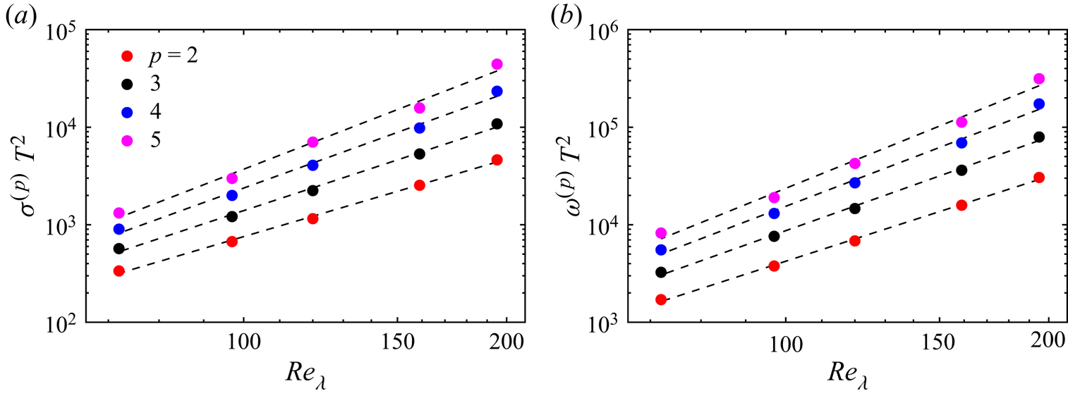
This implies that also  $\sigma ^{(p)}$ should follow a power-law scaling of the form $\omega ^{(p)}\sim Re_\lambda ^{\xi (p + 1) - \xi (p)}$. We corroborate this in figure 3(a), where we show $\sigma ^{(p)}$ as a function of $Re_\lambda$. In figure 3(b), we show that $\omega ^{(p)}$ follows a similar power-law scaling. This shows that our simulations, although of moderate Reynolds numbers, display intermittency effects characteristic of fully developed turbulence (Schumacher et al. Reference Schumacher, Scheel, Krasnov, Donzis, Yakhot and Sreenivasan2014).
Scaling of (a)  $\omega ^{(p)}$ and (b) $\sigma ^{(p)}$ with $Re_\lambda$. The dashed lines correspond to the least-squares fits of the data with a power law of the form $Re_\lambda ^{\xi }$, and $\omega ^{(p)}$ and $\sigma ^{(p)}$ are normalised with the integral eddy turnover time.
3. The temporal evolution of the generalised means
We study the evolution of the generalised means of the enstrophy and the strain for  $-4\leq p\leq 5$. In figure 4(a), we show the temporal evolution of $\varOmega ^{(3)}$, of the instantaneous space-averaged dissipation $\varepsilon$, and of the instantaneous surrogate dissipation $\varepsilon _s$, in a time interval of the simulation at $Re_\lambda =195$. To compare the three signals, we have subtracted their temporal mean and divided them by their standard deviation. The dissipation signal fluctuates around its mean in time scales comparable to the integral time scale, mirroring the fluctuations of the surrogate dissipation, which occur earlier. This time lag reflects the large-scale modulation of the small scales, which is a general feature of turbulent flows and has been observed previously in homogeneous flows (Kuczaj, Geurts & Lohse Reference Kuczaj, Geurts and Lohse2006; Chien, Blum & Voth Reference Chien, Blum and Voth2013), wall-bounded flows (Hutchins & Marusic Reference Hutchins and Marusic2007; Mathis, Hutchins & Marusic Reference Mathis, Hutchins and Marusic2009; Verschoof et al. Reference Verschoof, te Nijenhuis, Huisman, Sun and Lohse2018), and shear flows (Fiscaletti et al. Reference Fiscaletti, Attili, Bisetti and Elsinga2016; Lalescu & Wilczek Reference Lalescu and Wilczek2021). The time advancement of the surrogate dissipation with respect to the dissipation reflects the propagation of large-scale fluctuations down the energy cascade. This process takes place in local steps of duration proportional to the local eddy turnover time (Cardesa et al. Reference Cardesa, Vela-Martín, Dong and Jiménez2015), and is observable in a Lagrangian frame of reference Meneveau & Lund (Reference Meneveau and Lund1994), Wan et al. (Reference Wan, Xiao, Meneveau, Eyink and Chen2010) and Ballouz et al. (Reference Ballouz, Johnson and Ouellette2020). These cascade times are the same in linearly forced isotropic turbulence and in statistically steady homogeneous shear turbulence (Cardesa et al. Reference Cardesa, Vela-Martín, Dong and Jiménez2015), indicating that the temporal dynamics of the cascade is independent of the large-scale forcing mechanism. Thus, in our flow, the linear forcing provides a source of large-scale fluctuations, but should not affect the propagation of large-scale fluctuations down the cascade. Besides, our forcing scheme is not completely artificial; linearly forced isotropic turbulence is known to reproduce some of the dynamics of shear flows (Linkmann & Morozov Reference Linkmann and Morozov2015), and produces fluctuations of the surrogate dissipation that take place in a quasi-cyclic manner, reminiscent of the bursting phenomena in shear flows (Flores & Jiménez Reference Flores and Jiménez2010; Jiménez Reference Jiménez2013).
(a) Temporal evolution of the average energy dissipation  $\varepsilon (t)$, the surrogate energy dissipation $\varepsilon _s(t)$, and $\varOmega ^{(3)}(t)$, in the simulation at
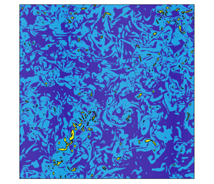
  $Re_{\lambda }=195$. Quantities are plotted without their temporal mean and divided by their standard deviation. (b) Visualisation of the enstrophy field in a plane of the flow for $Re_\lambda =195$. The yellow structures correspond to the most intense enstrophy that accounts for $90\,\%$ of $\langle \varOmega ^{3}\rangle$, and occupy approximately $1\,\%$ of the total volume. The light blue structures correspond to the most intense enstrophy that accounts for $90\,\%$ of $\langle \varOmega \rangle$, and the dark blue background corresponds to the remaining weak enstrophy that accounts for $10\,\%$ of $\langle \varOmega \rangle$. The plane shows the full computational domain, and the magenta line is equal to the instantaneous integral length scale, $L$.
$L$.

A relevant aspect of figure 4(a) is that  $\varOmega ^{(3)}$ is advanced with respect to $\varepsilon$, delayed with respect to $\varepsilon _s$, and largely correlated to both signals. The correlation between $\varepsilon$ and $\varOmega ^{(3)}$ is remarkable considering that the latter contains information on the evolution of only a very small fraction of the flow domain, which corresponds to events of intensity $\omega ^{(3)}\approx 70\overline {\langle \varOmega \rangle }$. A conservative measure of the volume covered by these events is given by
 \begin{equation} \upsilon^{(p)}(\varOmega)=\int_\chi^{\infty} P(\varOmega)\,\mathrm{d}\varOmega, \end{equation}
where  $\chi$ is such that
 \begin{equation} \int_{\chi}^{\infty} \varOmega^{p}\,P(\varOmega)\,\mathrm{d}\varOmega=0.9\overline{\langle \varOmega^{p} \rangle}. \end{equation}
The same definition holds for  $\varSigma$, denoted $\upsilon ^{(p)}(\varSigma )$. This quantity measures the average volume fraction occupied by the most intense events of $\varOmega$ and $\varSigma$ that account for $90\,\%$ of $\overline {\langle \varOmega ^{p}\rangle }$ and $\overline {\langle \varSigma ^{p}\rangle }$. In figure 4(b), we show the isocontours that enclose $\upsilon ^{(3)}(\varOmega )$ in a flow field at $Re_\lambda =195$. These isocontours correspond to the core of the most intense vortices, which occupy a volume fraction of $1\,\%$ of the flow domain ( $\upsilon ^{(3)}(\varOmega )\approx 0.01$), and appear distributed across the domain and separated by distances of the order of the integral scale (Jiménez et al. Reference Jiménez, Wray, Saffman and Rogallo1993). For comparison, we also show isocontours that enclose $90\,\%$ of the average enstrophy, which occupy $50\,\%$ of the domain ( $\upsilon ^{(1)}(\varOmega )\approx 0.5$). These strong differences suggest that $\varepsilon$ and $\varOmega ^{(3)}$ cannot be related directly. A plausible explanation for their temporal correlation comes from $\varepsilon _s$, which appears to be a precursor of both signals; large-scale fluctuations seem to modulate intense events in the same way that they modulate the average dissipation.
3.1. Temporal correlations of the generalised means
We study systematically the modulation of the  $p$-means and show that it is a persistent signature of the dynamics. We define the temporal cross-correlation coefficient of two test signals $\psi$ and $\phi$ as
 \begin{equation} \rho(\tau;\psi,\phi)=\frac{1}{T_{a}}\int{\psi'(t)\,\phi'(t + \tau)}\,\mathrm{d} t, \end{equation}
where  $\tau$ is a time shift, and the prime denotes quantities without temporal average, and normalised by their standard deviation. The integral is taken over an averaging time window of width $T_{a}$, which corresponds to the total signal length, $T_s$, except where $t+\tau$ is outside the signal boundaries. We denote the time shift at which the correlation is maximum as $\tau _{max}(\psi,\phi )$, and the maximum value of the correlation as $\rho _{max}(\psi,\phi )=\rho (\tau _{max};\psi,\phi )$.
We focus now on the values of the maximum correlation coefficient. In figures 5(a,b), we show the joint p.d.f.s of  $\varepsilon '$ and ${\varOmega ^{(p)}}'$, and $\varepsilon '$ and ${\varSigma ^{(p)}}'$, for $p=3$ and $p=5$, and $Re_\lambda =195$. Here, $\varepsilon '$ has been time-shifted by $\tau _{max}(\varOmega ^{(p)},\varepsilon )$ and $\tau _{max}(\varSigma ^{(p)},\varepsilon )$, respectively. The correlation observed in figure 4(a) is verified here for the full time series. For $p=3$, the p.d.f.s are very similar for $\varOmega ^{(3)}$ and $\varSigma ^{(3)}$, and they are centred around the line of best least-squares fit, whose slope is equal to $\rho _{max}$. The maximum correlation coefficients are approximately $0.85$ for both $\varOmega ^{(3)}$ and $\varSigma ^{(3)}$. For $p=5$, the correlation coefficients decrease to approximately $0.6$ for both $\varOmega ^{(5)}$ and $\varSigma ^{(5)}$. In figures 5(c,d), we show the same p.d.f.s as in figures 5(a,b), but comparing with the surrogate energy dissipation. The values of the correlation maxima are similar to those calculated with the dissipation, although slightly lower. They are around $0.7$ for $p=3$, and $0.5$ for $p=5$, for both $\varOmega ^{(p)}$ and $\varSigma ^{(p)}$. This similarity is not surprising if we consider that $\varepsilon _s$ and $\varepsilon$ are highly correlated (with a time shift): $\rho _{max}(\varepsilon,\varepsilon _s)\approx 0.95$ for all $Re_\lambda$.
(a,b) Joint p.d.f. of  $\varepsilon '(t + \tau _{max})$ and ${\varOmega ^{(p)}}'(t)$, and $\varepsilon '(t + \tau _{max})$ and ${\varSigma ^{(p)}}'(t)$, for (a) $p=3$ and (b) $p=5$ at $Re_\lambda =195$. These quantities are normalised by subtracting their temporal mean, and dividing by their standard deviation, and $\tau _{max}$ is the time shift for which the correlation between $\varepsilon$ and $\varOmega ^{(p)}$ or $\varSigma ^{(p)}$ is maximum. The lines corresponds to the linear least-squares fits of the data for (solid) $\varOmega ^{(p)}$, and (dashed) $\varSigma ^{(p)}$. (c,d) Similar to (a,b), but for the surrogate energy dissipation, $\varepsilon _s$. (e) Maximum temporal correlation coefficient of (empty symbols) $\phi =\varOmega ^{(p)}$ and (solid symbols) $\phi =\varSigma ^{(p)}$ with $\varepsilon$ as a function of $p$ for different Reynolds numbers. Empty symbols correspond to $\psi =\varOmega ^{(p)}$, and solid symbols to $\psi =\varSigma ^{(p)}$. (f) Maximum temporal correlation coefficient of $\varOmega ^{(p)}$ and $\varSigma ^{(p)}$ for $p=5$ as a function of $Re_\lambda$. Symbols as in (e).
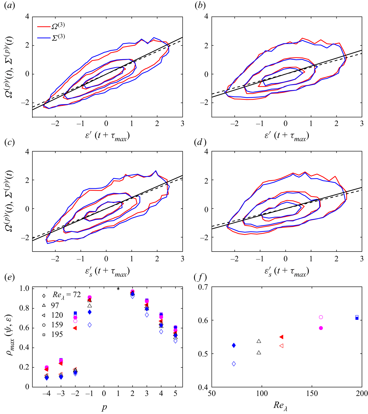
In view of these results, we analyse now the maximum correlation coefficient between the generalised means and the dissipation signal. This analysis yields qualitatively similar results when applied to the surrogate dissipation. In figure 5(e), we show the maximum value of the correlation  $\rho _{max}(\varOmega ^{(p)},\varepsilon )$ and $\rho _{max}(\varSigma ^{(p)},\varepsilon )$ for different values of $p$ and $Re_\lambda$. The maxima are similar for $\varOmega ^{(p)}$ and $\varSigma ^{(p)}$, and decay for increasing $p$. That the correlation is of the order of $0.5$ for $p=5$ is significant considering the small support in physical space of $\varOmega ^{(5)}$ and $\varSigma ^{(5)}$. For $Re_\lambda =195$, $\upsilon ^{(5)}(\varOmega )\approx 10^{-4}$, i.e. the events represented by $\varOmega ^{(5)}$ occupy approximately $0.01\,\%$ of the total flow domain ( $\varSigma ^{(5)}$ yields comparable results). Yet the evolution of these very intense events – $\omega ^{(5)}\approx 400\overline {\langle \varOmega \rangle }$ and $\sigma ^{(5)}\approx 100\overline {\langle \varSigma \rangle }$ – is correlated to the dissipation signal. In figure 5(e), we have also included the maximum correlation coefficient for $p<0$ to show that the weak turbulent background is less correlated to the average dissipation than the intense events. These results are in agreement with Vela-Martín (Reference Vela-Martín2021), who showed that weak vorticity is less tuned to inertial-range fluctuations than intense vorticity. This also suggests that the non-vanishing correlations for large $p$ are not a statistical artefact, and reflects the control exerted by inertial scales on the intense events of the dissipation and the enstrophy. Finally, in figure 5(f), we show that $\rho _{max}(\varSigma ^{(5)},\varepsilon )$ increases with $Re_\lambda$, and that $\rho _{max}(\varOmega ^{(5)},\varepsilon )$ plateaus for $Re_\lambda >120$, suggesting that the correlations analysed here should persist at higher $Re_\lambda$, and that they are not a finite-Reynolds-number effect.
3.2. Time lags between the generalised means and the dissipation
We now focus on the time lags that yield the maximum correlation, and show that the temporal advancement of  $\varOmega ^{(3)}$ with respect to the dissipation observed in figure 4(a) is a persistent feature, which is captured by the temporal correlations.
In figure 6(a), we show  $\rho (\tau ;\varOmega ^{(p)},\varepsilon$) divided by its maximum as a function of $\tau$ for different values of $p$. The time shift at which the correlation peaks, $\tau _{max}$, is positive for $p>1$, indicating that the fluctuations of intense events precede, on average, the dissipation signal. This temporal advancement grows with increasing $p$. On the other hand, for $p=-1$, the $p$-means are delayed with respect to the average dissipation.
(a) Correlation coefficient of  $\varOmega ^{(p)}$ with $\varepsilon$ as a function of the time shift, $\tau$, divided by its maximum value, $\rho _{max}(\varOmega ^{(p)},\varepsilon )$, for different $p$. The Reynolds number is $Re_\lambda =195$. The solid lines with markers correspond to: magenta squares, $p=-1$; red circles, $p=3$; blue diamonds, $p=5$. The dashed line corresponds to the temporal autocorrelation of $\varepsilon$, namely $\rho (\tau ;\varepsilon,\varepsilon )$. (b) Same as in (a) but with the surrogate dissipation. Here the dashed line corresponds to the cross-correlation $\rho (\tau ;\varepsilon,\varepsilon _s)$. (c) Advancement of the generalised means with respect to the dissipation, (solid symbols) $\tau _{max}(\varOmega ^{(p)},\varepsilon )$ and (empty symbols) $\tau _{max}(\varSigma ^{(p)},\varepsilon )$ as functions of the inverse of the characteristic turnover time, $t_\omega ^{(p)}$ and $t_\sigma ^{(p)}$, for different Reynolds numbers. The colours correspond to: black, $p=2$; red, $p=3$; magenta, $p=4$; blue, $p=5$. The error bars mark the standard deviation of the data obtained by dividing the temporal signal in four subsets. (d) Advancement of the generalised means with respect to the dissipation measured from the surrogate dissipation, $\tau ^{+}_{max}$ (colour symbols) for $C_+=0.61$ (see (3.4)). The styles and colours of the symbols are similar to those in (c), and only data from $Re_\lambda =195$ and $120$ have been plotted for ease of comparison. The symbols in grey correspond to the data in (c).

In figure 6(b), we show the same time lags but with respect to  $\varepsilon _s$. Here, $\tau _{max}$ is negative, meaning that the generalised means are delayed with respect to the surrogate dissipation. This delay now decreases for increasing $p$, in agreement with the results in figure 6(a); the higher the advancement of the generalised means with respect to the dissipation, the shorter the time delay with respect to the surrogate dissipation. For $p=0$, we recover the temporal cross-correlation between $\varepsilon$ and $\varepsilon _s$, which peaks at around one integral eddy turnover time. This is consistent with the cascade time of the large-scale eddies in the classical picture of the energy cascade.
We calculate  $\tau _{max}$ carefully by fitting each correlation around its maximum with a third-order polynomial, and taking $\tau _{max}$ as the time where the polynomial is maximum. In figure 6(c), we plot $\tau _{max}(\varOmega ^{(p)},\varepsilon )$ and $\tau _{max}(\varSigma ^{(p)},\varepsilon )$ for $p>1$ against the inverses of $t_\omega ^{(p)}$ and $t_\sigma ^{(p)}$ (see (2.14)), and normalise all quantities by the integral eddy turnover time. The advancements of $\varOmega ^{(p)}$ and $\varSigma ^{(p)}$ with respect to the dissipation collapse well with this normalisation, and $\tau _{max}$ seems to grow quasi-logarithmically with the inverses of $t_\sigma ^{(p)}$ and $t_\omega ^{(p)}$. Only the data for $p=2$ and large Reynolds numbers deviate from the mean scaling. We will give a possible explanation for this in the next section. In summary, the data reveal that the more intense the events tracked by the $p$-means, the shorter their characteristic turnover time, and the more advanced their signals are with respect to the dissipation.
We repeat this analysis with respect to the surrogate dissipation, and obtain a similar scaling. It is reasonable to assume that the time shifts of the maximum correlations are additive,  $\tau _{max}(\psi,\varepsilon )=\tau _{max}(\psi,\varepsilon _s) + \tau _{max}(\varepsilon _s,\varepsilon )$, but this is not the case. Instead, the relation that holds is one of proportionality, $\tau _{max}(\psi,\varepsilon )\approx C_+(\tau _{max}(\psi,\varepsilon _s) + \tau _{max}(\varepsilon _s,\varepsilon ))$. We define the time advancement of the generalised means with respect to $\varepsilon$ measured from the large scales as
 \begin{equation} \tau^{+}_{max}(\psi,\varepsilon)=C_+(\tau_{max}(\psi,\varepsilon_s) + \tau_{max}(\varepsilon_s,\varepsilon)), \end{equation}
where  $C_+=0.61$ corresponds to the best fit of $\tau ^{+}_{max}(\psi,\varepsilon )$ to $\tau _{max}(\psi,\varepsilon )$ with our data. In figure 6(d), we have plotted $\tau ^{+}_{max}(\psi,\varepsilon )$ over $\tau _{max}(\psi,\varepsilon )$ to show that both quantities collapse fairly well for different values of $p$.
$p$.
The meaning of the proportionality constant is not obvious, but suggests that the estimate in the time lags between signals provided by the cross-correlations is only approximate, and, in any case, an average measure. The time lags are surely sensitive to the degree of correlation, and the slightly lower values of  $\rho _{max}(\varOmega ^{(p)},\varepsilon _s)$ and $\rho _{max}(\varSigma ^{(p)},\varepsilon _s)$ with respect to $\rho _{max}(\varOmega ^{(p)},\varepsilon )$ and $\rho _{max}(\varSigma ^{(p)},\varepsilon )$ may be the source of this discrepancy (see § 3.1). Yet let us note that $C_{+}$ introduces a correction to $\tau _{max}(\psi,\varepsilon _s) + \tau _{max}(\varepsilon _s,\varepsilon )$ of between $5$% and $30$% of $T$. This is not large compared to $\tau _{max}(\varepsilon,\varepsilon _s)$, which is of the order of $T$. In any case, the scaling of $\tau _{max}(\psi,\varepsilon _s) + \tau _{max}(\varepsilon _s,\varepsilon )$ with the intensity of the generalised means is similar to that of $\tau _{max}(\psi,\varepsilon )$ (save for the proportionality constant, $C_+$), suggesting that the time lags are a robust feature of the flow that can be measured from either the large scales or the dissipative range.
4. Cascade times in a multiplicative model
In this section, we elaborate on a possible explanation for the results presented in the previous sections. We will show that the time advancement of the generalised means is consistent with a local energy cascade, in which eddies cascade in a time proportional to their turnover time, causing intense eddies to reach the dissipative scales before the average energy dissipation. We will argue that the logarithmic scaling of  $\tau _{max}$ with the turnover time of intense eddies is a consequence of an accumulative process taking place through the cascade.
Let us consider the binomial model of Meneveau & Sreenivasan (Reference Meneveau and Sreenivasan1987), which describes a cascade with average energy flux  $\mathcal {E}$ in a one-dimensional domain of size $\mathcal {L}$ . The one-dimensional domain is valid for the purpose of this analysis, and we consider it here for simplicity. The process starts with the largest eddy of size $\mathcal {L}_0=\mathcal {L}$ and energy flux $\mathcal {E}_0=\mathcal {E}$. Here the energy flux can be regarded as a measure of the intensity of the eddy. At the $n$th step of the cascade, each eddy is divided into two eddies of similar size, $\mathcal {L}_{n+1}=\mathcal {L}_{n}/2$, and its intensity, $\mathcal {E}_n$, is distributed conservatively between the two eddies with a fraction of either $\varPi =0.7$ or $1-\varPi =0.3$ (Meneveau & Sreenivasan Reference Meneveau and Sreenivasan1987). These fractions are assigned randomly. The intensities of the new eddies are $\mathcal {E}_{n+1,2m}=2 \varPi \mathcal {E}_{n,m}$ and $\mathcal {E}_{n+1,2m+1}=2(1-\varPi )\mathcal {E}_{n,m}$. Here, the second subindex denotes the position of the eddy in a one-dimensional grid with $m=0,\dots,2^{n}-1$ points. At each level, there are $2^{n}$ eddies. Thus at the $n$th step of the cascade, the intensity of an eddy is the product of $n$ random multipliers (either $0.3$ or $0.7$),
 \begin{equation} \mathcal{E}_{n,m}=2^{n}\varPi^{n-l}(\varPi-1)^{l}\mathcal{E}, \end{equation}
where  $l$ is a random integer such that $0\leq l \leq n$. The cascade continues down to the Kolmogorov scale, $\eta /\mathcal {L}\sim ({1}/{2})^{q}$, where $q$ is the total number of steps of the cascade. This simple multiplicative cascade process reproduces accurately the intermittent structure of the dissipation field, yielding a spectrum of generalised dimensions that is very well in agreement with experimental and numerical data (Meneveau & Sreenivasan Reference Meneveau and Sreenivasan1987, Reference Meneveau and Sreenivasan1991).
Although this model is geometrical and provides only a frozen picture of turbulence, it contains some dynamical aspects that can be leveraged to explain the main results of this paper. More specifically, we assume that the cascade time of eddies is proportional to their turnover time. This relation is one of the cornerstones of the classical theory of the cascade, and is known to hold locally in turbulent flows (Meneveau & Lund Reference Meneveau and Lund1994; Wan et al. Reference Wan, Xiao, Meneveau, Eyink and Chen2010; Ballouz et al. Reference Ballouz, Johnson and Ouellette2020). In the  $n$th cascade step, the cascade time of an eddy of intensity $\mathcal {E}_{n,j}$ is
 \begin{equation} t_{n,j}=C_{T}\left(\frac{\mathcal{L}_n^{2}}{\mathcal{E}_{n,j}}\right)^{1/3}, \end{equation}
where  $C_{T}$ is a proportionality constant. The cascade time of a single eddy to step $s$ is
 \begin{equation} \mathcal{T}_{s,j}=\sum_{n=0}^{s-1} t_{n,j}=C_{T}\sum_{n=0}^{s-1}\left(\frac{\mathcal{L}_n^{2}}{\mathcal{E}_{n,j}}\right)^{1/3}, \end{equation}
and the average cascade time to scale  $s$ is
 \begin{equation} \{\mathcal{T}\}_s=\frac{1}{2^{s}}\sum_{j=0}^{2^{s}-1} \mathcal{T}_{s,j}. \end{equation}
Introducing cascade times does not change the geometrical essence of the model, but leads naturally to fluctuations in the time it takes for eddies to reach the dissipative scales. This is so because, as shown by (4.2), the more intense an eddy, the shorter its cascade time and the faster it reaches the dissipative scales with respect to the average. We will see that this simple approach provides a dynamical framework that explains the results presented in the previous sections.
We have simulated a random cascade process with  $q=12$, which corresponds to $Re_\lambda \approx 200$ (Meneveau & Sreenivasan Reference Meneveau and Sreenivasan1987), and that produces a total of $2^{12}=4096$ different eddies. In figure 7(a), we show two typical realisations of this random process, where the effect of multiplicative amplification is evident in the large spikes of $\mathcal {E}_{q,j}$. Figure 7(b) shows the cascade times to scale $q$,
$q$,  $\mathcal {T}_{q,j}$, of each eddy for the same two realisations. We have chosen $C_T=0.4$ (this will be justified later). There is a noticeable deviation of the cascade times with respect to the mean cascade time. We have marked the maxima of $\mathcal {E}_{q,j}$ in figure 7(a), and their corresponding cascade times in figure 7(b), to show that the most intense eddies cascade the fastest.
(a) Two realisations of the binomial cascade model for  $q=12$ ( $Re_\lambda \approx 200$), where $x_j$ denotes the positions of $\mathcal {E}_{q,j}$. The maxima of $\mathcal {E}_{q,j}$ in each realisation are marked with circles. (b) Cascade times $\mathcal {T}_{q,j}$ of each eddy for the same realisations of the cascade model as in (a). The circles correspond to the maxima of $\mathcal {E}_{q,j}$ in (a). (c) Histogram of the cascade times $\mathcal {T}_{q,j}$ of eddies of equal intensities $\mathcal {E}_{\{r\}}$. Here, $T=(\mathcal {L}^{2}/\mathcal {E})^{1/3}$ is the integral eddy turnover time of the model. The total number of eddies is $2^{12}=4096$. In (b) and (c), the proportionality constant of the cascade time is set to $C_T=0.4$. (d) As in figure 6(c), where the solid black line corresponds to $\tau _{\{r\}}/T$ as a function of $T/t_{\{r\}}$ derived from a binomial cascade model.

Since the intensities of the eddies are a product of random multipliers with fixed values ( $0.3$ or $0.7$), and these multipliers commute, many of these eddies have the same intensities. In fact, at the last stage there are only $q+1=13$ distinct intensities, which we denote by $\mathcal {E}_{\{r\}}$, where $r=0,\ldots,12$. Thus we group the eddies with equal intensities in $13$ sets, and estimate the total cascade time associated with each intensity as the average of $\mathcal {T}_{q,j}$ in the set, denoted by
 \begin{equation} \mathcal{T}_{\{r\}}=\frac{1}{\mathcal{N}(r)}\sum_{\mathcal{E}_{q,j}=\mathcal{E}_{\{r\}}} \mathcal{T}_{q,j}, \end{equation}
where the summation is taken over eddies that have an intensity at the final level,  $\mathcal {E}_{q,j}$, similar to $\mathcal {E}_{\{r\}}$, and $\mathcal {N}(r)$ is the number of eddies that have intensity $\mathcal {E}_{\{r\}}$. We perform this average because the cascade times, unlike the intensities, depend on the order in which the multipliers are applied. Thus eddies with the same intensity may have different cascade times. In figure 7(c), we show the histograms of the cascade times for four different sets of eddies. For each value of $\mathcal {E}_{\{r\}}$, there exists a wide range of cascade times. As $\mathcal {E}_{\{r\}}$ increases, the cascade time becomes predominantly shorter than the average cascade time. Conversely, low values of $\mathcal {E}_{\{r\}}$ lead in general to slower eddies that reach the dissipative scales later.
In order to compare the cascade times of this model with the results of the direct numerical simulations, we define the advancement of eddies of intensity  $\mathcal {E}_{\{r\}}$ with respect to the average cascade time as
 \begin{equation} \tau_{\{r\}}=\{\mathcal{T}\}_q-\mathcal{T}_{\{r\}}. \end{equation}
We associate the intensity of each set of eddies,  $\mathcal {E}_{\{r\}}$, with $\sigma ^{(p)}$, and define the characteristic turnover time of each set as
 \begin{equation} t_{\{r\}}=\sqrt{\frac{\nu_q}{\mathcal{E}_{\{r\}}}}, \end{equation}
where  $\nu _q$ is a prescribed kinematic viscosity of the model. These quantities are the equivalent in our model of $\tau _{max}(\varSigma ^{(p)},\varepsilon )$ and $t_\sigma ^{(p)}$ in the direct numerical simulations.
In figure 7(d), we have plotted  $\tau _{\{r\}}/T$ as a function of $T/t_{\{r\}}$ on top of $\tau _{max}(\varSigma ^{(p)},\varepsilon )/T$, and $T/t_\sigma ^{(p)}$. We define the integral turnover time of the model as $T=(\mathcal {L}^{2}/\mathcal {E})^{1/3}$. With $C_{T}=0.4$ and $\nu _q T/\mathcal {L}^{2}=1.3\times 10^{-3}$, the cascade model yields results that are in good qualitative agreement with the data obtained from the direct numerical simulations. We do not make any claim here on the quantitative agreement because $C_T$ has to be slightly modified to produce a similarly good fit when the Reynolds number of the model ( $q$) is changed. Nevertheless, the value of $C_T$ is not completely arbitrary but yields an average cascade time $\{\mathcal {T}\}_q=1.15T$. This is very close to the values obtained in the direct numerical simulations for $\tau _{max}(\varepsilon _s,\varepsilon )$, which may be interpreted as the average cascade time. Here, $\nu _q$ has to be tuned so that $\mathcal {E}_{\{r\}}$ is similar to $\sigma ^{(p)}$. Note that in the direct numerical simulations at $Re_\lambda =195$, $\nu T/\bar {L}^{2}=4\times 10^{-4}$, which is reasonably close to $\nu _q T/\mathcal {L}^{2}=1.3\times 10^{-3}$. These discrepancies are not surprising given our crude approach. Yet these results are remarkable considering that we have added to the model only the assumption that eddies cascade in a time proportional to their eddy turnover time.
A relevant aspect of the approach followed here is that it provides a plausible explanation for the logarithmic growth of  $\tau _{max}$. In figure 8(a), we show four different paths followed by eddies in the flux-scale phase space, where each circle corresponds to an admissible state $\mathcal {E}_{n}$, and we have dropped the position index $j$ for simplicity. The evolution of each eddy may be regarded as a random walk in this space, in which, due to the multiplicative nature of the model, the accessible states are equispaced in a logarithmic mesh. This means that $\mathcal {E}_n$ may grow exponentially with $n$ (or linearly with the inverse of $\mathcal {L}_n=\mathcal {L}/2^{n}$), as in the case of the most amplified eddy in a realisation, $\mathcal {E}_n=1.4^{n}\mathcal {E}$. On the other hand, the time advancements are a sum of time increments, and can grow at most linearly, but for only a few steps of the cascade. In figure 8(b), we show the time advancement due to each step of the cascade,
 \begin{equation} \tau_{n}= \{\mathcal{T}\}_{n} - \mathcal{T}_n, \end{equation}
where we have dropped the position index. The lines in figure 8(b) correspond to the same individual paths as in figure 8(a). The growth of the time advancements is predominantly sub-linear, and occurs mostly in the first steps of the cascade. Taking the most amplified eddy as a reference, its intensity grows exponentially with  $n$, but its advancement with respect to the average cascade time grows linearly only until $n=5$, and then sub-linearly. For these first steps, $\tau _n\sim n$, $\mathcal {E}_n\sim 1.4^{n}$ and $\tau _n\sim \log \mathcal {E}_n$. This expression explains partly the good fit of the model in figure 8(d), and provides a good account for the scaling of $\tau _{max}$. For low values of $\mathcal {E}_q$, the growth of $\tau _n$ will be markedly sub-linear (see the magenta line in figures 8a,b). This may explain why $\tau _{max}$ for $p=2$ (which targets not-so-intense events) in figure 6(c) deviates from the scaling at large $p$. A possible fit for the magenta line is $\tau _n\sim \log n$ or $\tau _n\sim n^{\gamma }$, where $\gamma <1$, and thus $\tau _n \sim \log \log \mathcal {E}_n$ or $\tau _n \sim \log ^{\gamma } \mathcal {E}_n$.
(a) Four different amplification paths of  $\mathcal {E}_n$ in scale space. Each line corresponds to a different eddy in the same realisation of the binomial cascade model. The circles correspond to the accessible states that allow for $\mathcal {E}_q>\mathcal {E}$. The black solid line corresponds to the most amplified eddy in the realisation. (b) Advancement of the cascade time with respect to the average cascade time $\tau _n$ at each step $n$ of the cascade, for the same paths as in (a).

Let us remark that this model predicts that the time advancements should saturate progressively for higher Reynolds numbers ( $q \rightarrow \infty$), where the maximum value of the advancement is $\tau _n\approx 0.25T$ for the most intense eddy. This is something that we do not observe clearly in our simulations, probably due to the moderate Reynolds numbers, but that should be examined with new simulations at higher Reynolds numbers.
5. Conclusion
We have studied the dynamics of intense events using the generalised means of the enstrophy and the strain in direct numerical simulations of isotropic turbulence. We have shown that the evolution of these signals, which track the intense events, is correlated to large-scale fluctuations, and that, on average, the fluctuations of the intense events occur before the fluctuations of the average dissipation. Correlation does not, in general, imply causation, except in the case of strongly unidirectionally coupled systems (Ye et al. Reference Ye, Deyle, Gilarranz and Sugihara2015). Recent synchronisation experiments have shown that this is the case in isotropic turbulence (Vela-Martín Reference Vela-Martín2021), in which inertial-range dynamics controls intense events in the dissipative scales in a master–slave scenario. In this light, we state that the correlations reported here reflect the causal influence of the large scales on the intense events of the enstrophy and the dissipation through the energy cascade.
This claim is supported on two observations. First, the temporal correlation between the average dissipation signal – and its large-scale surrogate – and the most intense events is hard to explain without the cascade. That a few small-scale structures separated by distances of the order of the integral scale (see figure 4b) follow an organised temporal evolution is conceivable only if they emerge from the same large-scale event, which reaches the dissipative scales through the cascade. Second, the temporal advancement of the generalised means suggests that intense events are caused by fluctuations that precede the average dissipation signal, namely fluctuations at inertial scales (Cardesa et al. Reference Cardesa, Vela-Martín, Dong and Jiménez2015).
We have shown that the growth of the time advancement with the intensity of the generalised means is consistent with a multiplicative cascade, and can be reproduced qualitatively using the multifractal cascade model of Meneveau & Sreenivasan (Reference Meneveau and Sreenivasan1987), under the assumption that eddies cascade in a time proportional to their turnover time. The more amplified an eddy, the faster it cascades to smaller scales, thus advancing the average dissipation. We have shown that this effect is accumulated through the cascade, explaining the logarithmic scaling of the time advancements with the intensity of the events. By the same token, this model also predicts that eddies that are weaker than the average energy flux (dissipation) take longer to reach the dissipative scales. This is in agreement with the data in figure 6(b), which show that the generalised means for  $p<1$ are delayed with respect to the average dissipation.
These results connect the dynamics of intense and extreme events in small-scale turbulence to the energy cascade, and evidence that the phenomenological picture conveyed by multiplicative cascade models is plausible, i.e. that of an energy cascade in which eddies are amplified as they ‘break’, leading to intense events of the dissipation and the enstrophy once these eddies reach the Kolmogorov scale. These results open the possibility to improve multiplicative models by including temporal dynamics that can reproduce the observations presented here in a consistent way.
Multiplicative cascade models provide a very coarse-grained account of the physics of turbulence, yet they are constructed in terms of objects – scales, eddies and energy fluxes – that create a simple, intuitive and powerful picture. This is, besides their predictive value, one of their strengths. Turbulent flows can be probed in search of approximate representations of these objects based on measurable quantities. Elucidating the dynamics of these objects is beyond the scope of multiplicative models, since it is clear that their coarse-grained nature allows for different possible underlying dynamics. In this sense, here we have presented evidence that the evolution of intense events in the dissipative range may be explained by a cascade process with a multiplicative footprint. The exact details of this process, i.e. the mechanisms of interscale energy transfer, are not fully understood, and their study is part of the ongoing research by the turbulence community.
A possible extension of this work is to track intense events through the cascade in the spirit of Lozano-Durán & Jiménez (Reference Lozano-Durán and Jiménez2014) and Cardesa et al. (Reference Cardesa, Vela-Martín and Jiménez2017). This poses many challenges; perhaps the most problematic is defining the quantities that can describe properly the dynamics of the inertial range in a local manner. The filtered velocity gradients are definitely not good candidates, since their squares are not conserved through the cascade. The local interscale energy fluxes may be a good choice, but they are subject to local gauge ambiguities (Jimenez Reference Jimenez2017), which should be resolved from physical grounds. This endeavour seems necessary to clarify fully the dynamical processes behind intermittency, and intense and extreme events, in small-scale turbulence.
Declaration of interests
The author reports no conflict of interest.


 Open access