


1. Introduction
Waves are ubiquitous in rotating and stratified fluids. They play a key role in the dynamics of both the ocean (Munk & Wunsch Reference Munk and Wunsch1998) and the atmosphere (Fritts & Alexander Reference Fritts and Alexander2003). In the ocean, such waves can be generated by tidal flows interacting with topography (Wunsch Reference Wunsch1975). When the topography is supercritical, that is, when it has a slope tangent to the direction of wave propagation, concentrated wave beams are emitted from so-called critical (slope) points. These beams have been studied both experimentally (Zhang, King & Swinney Reference Zhang, King and Swinney2007; King, Zhang & Swinney Reference King, Zhang and Swinney2009; Echeverri & Peacock Reference Echeverri and Peacock2010) and theoretically (St Laurent et al. Reference St. Laurent, Stringer, Garrett and Perrault-Joncas2003; Llewellyn Smith & Young Reference Llewellyn Smith and Young2003; Balmforth & Peacock Reference Balmforth and Peacock2009) in this context. Similar concentrated beams also occur in rotating fluids (Greenspan Reference Greenspan1968). They have often been investigated in spherical geometries (Calkins et al. Reference Calkins, Noir, Eldredge and Aurnou2010; Koch et al. Reference Koch, Harlander, Egbers and Hollerbach2013; Cébron et al. Reference Cébron, Laguerre, Noir and Schaeffer2019; Lin & Noir Reference Lin and Noir2021; He et al. Reference He, Favier, Rieutord and Le Dizès2022, Reference He, Favier, Rieutord and Le Dizès2023) due to their relevance in planetary and stellar interiors (Le Bars, Cébron & Le Gal Reference Le Bars, Cébron and Le Gal2015). Their structure has been examined theoretically in works such as Walton (Reference Walton1975), Kerswell (Reference Kerswell1995), Tilgner (2000) and more recently in Le Dizès & Le Bars (Reference Le Dizès and Le Bars2017).
The theoretical description of these beams is based on the similarity solutions obtained by Moore & Saffman (Reference Moore and Saffman1969) for rotating fluids and Thomas & Stevenson (Reference Thomas and Stevenson1972) for stratified fluids. These asymptotic viscous solutions have primarily been used to describe wave fields far from a localised oscillating source (Hurley & Keady Reference Hurley and Keady1997; Voisin Reference Voisin2003; Cortet, Lamriben & Moisy Reference Cortet, Lamriben and Moisy2010; Machicoane et al. Reference Machicoane, Cortet, Voisin and Moisy2015). They are parametrised by an index $m$
, which characterises the strength of the underlying inviscid singularity. Only recently have these solutions been applied to describe the concentrated beams issued from critical points (Le Dizès & Le Bars Reference Le Dizès and Le Bars2017; He et al. Reference He, Favier, Rieutord and Le Dizès2022, Reference He, Favier, Rieutord and Le Dizès2023; Le Dizès Reference Le Dizès2024). Furthermore, Ogilvie (Reference Ogilvie2005) and He et al. (Reference He, Favier, Rieutord and Le Dizès2023) have shown that these solutions can also describe the asymptotic viscous structure of the internal shear layers associated with wave attractors.
$m$
, which characterises the strength of the underlying inviscid singularity. Only recently have these solutions been applied to describe the concentrated beams issued from critical points (Le Dizès & Le Bars Reference Le Dizès and Le Bars2017; He et al. Reference He, Favier, Rieutord and Le Dizès2022, Reference He, Favier, Rieutord and Le Dizès2023; Le Dizès Reference Le Dizès2024). Furthermore, Ogilvie (Reference Ogilvie2005) and He et al. (Reference He, Favier, Rieutord and Le Dizès2023) have shown that these solutions can also describe the asymptotic viscous structure of the internal shear layers associated with wave attractors.
Most of the existing studies have focused on uniformly rotating and stratified fluids. In a non-uniform medium, the direction of wave propagation is expected to vary with position. In such cases, a local wave analysis is typically employed, based on Wentzel–Kramers–Brillouin (WKB) approximations and ray tracing techniques (Lighthill Reference Lighthill1978; Marks & Eckermann Reference Marks and Eckermann1995; Broutman, Rottman & Eckermann Reference Broutman, Rottman and Eckermann2004; Prat, Lignières & Ballot Reference Prat, Lignières and Ballot2016; Prat et al. Reference Prat, Mathis, Augustson, Lignières, Ballot, Alvan and Brun2018). Rays may, in particular, encounter points where they can no longer propagate. At these so-called turning points, the rays reflect and form a typical cusp structure Friedlander & Siegmann (Reference Friedlander and Siegmann1982). The wave solution near turning points is expected to be described by an Airy equation; see Wasow (Reference Wasow1985) and Sutherland (Reference Sutherland2010). The local wave approach has helped explain various features observed in the structure of free oscillating modes in closed geometries; see Dintrans, Rieutord & Valdettaro (Reference Dintrans, Rieutord and Valdettaro1999), Maas (Reference Maas2001), Harlander & Maas (Reference Harlander and Maas2007), Mathis (Reference Mathis2009), Baruteau & Rieutord (Reference Baruteau and Rieutord2013), Guenel et al. (Reference Guenel, Baruteau, Mathis and Rieutord2016), Mirouh et al. (Reference Mirouh, Baruteau, Rieutord and Ballot2016) and Astoul et al. (Reference Astoul, Park, Mathis, Baruteau and Gallet2021).
The concentrated beams generated from critical or singular points are small-scale structures, for which this local wave approach is expected to be applicable. We will show that the similarity solution of Moore & Saffman (Reference Moore and Saffman1969) remains valid in a non-uniform medium, provided the beam width is small compared with the spatial scale associated with the varying background. The same conclusion was reached by Kistovich & Chashechkin (Reference Kistovich and Chashechkin1998) for non-rotating fluids. The beam’s width and amplitude vary according to the local properties of the medium. We will demonstrate that the similarity solution breaks down at the turning point. A new local solution will be constructed to describe the beam behaviour near this point, showing that the beam reflects while maintaining its similarity structure and acquiring a phase shift of $\pm \pi /2$
, as for non-rotating fluids (Kistovich & Chashechkin Reference Kistovich and Chashechkin1998). These theoretical predictions are validated using numerical simulations of the linear governing equations.
$\pm \pi /2$
, as for non-rotating fluids (Kistovich & Chashechkin Reference Kistovich and Chashechkin1998). These theoretical predictions are validated using numerical simulations of the linear governing equations.
The paper is organised as follows. Section 2 presents the general framework. We consider a non-uniform axisymmetric medium in which the angular velocity varies with the cylindrical radius and the Brunt–Väisälä frequency varies with the spherical radius. The governing equations, ray equations and local dispersion relations are provided in this section. We also derive the form of the governing equations in the local Frenet–Serret frame attached to a given characteristic. Section 3 uses these equations to obtain an asymptotic solution describing viscous wave beams concentrated along a characteristic. The classical similarity solution of Moore & Saffman (Reference Moore and Saffman1969) is recovered as one possible solution. Section 4 analyses the behaviour of the viscous solution near a turning point. The appropriate scalings, the local governing equation and its solution are derived. Section 5 presents the numerical validation of the theory. Simulations are conducted in a finite domain with a non-stratified configuration, using a localised forcing to generate the concentrated beam and sponge layers to prevent boundary reflections. The structure of the solution, both near and far from the turning point, is compared with the theoretical predictions. Finally, in the conclusion, we summarise the results and discuss their possible extension to finite geometries.
2. Framework
We consider an incompressible fluid undergoing differential rotation about the vertical axis $Oz$
, with an angular velocity
$Oz$
, with an angular velocity $\varOmega (r)$
that depends only on the cylindrical radial coordinate
$\varOmega (r)$
that depends only on the cylindrical radial coordinate $r$
. The fluid is also assumed to be stably stratified in a central gravitational field, with a Brunt–Väisälä frequency
$r$
. The fluid is also assumed to be stably stratified in a central gravitational field, with a Brunt–Väisälä frequency $N(\rho )$
that depends solely on the spherical radial coordinate
$N(\rho )$
that depends solely on the spherical radial coordinate $\rho$
. The kinematic viscosity
$\rho$
. The kinematic viscosity $\nu$
and the scalar diffusivity
$\nu$
and the scalar diffusivity $\alpha$
are both taken to be constant. The model chosen for the stratification and angular rotation mimics configurations that can be found in stellar interiors (e.g. Dintrans et al. Reference Dintrans, Rieutord and Valdettaro1999). It can be rigorously justified provided that the centrifugal force remains negligible compared with gravity. However, this is not our purpose here, as other models can be adapted to the following derivation without difficulty.
$\alpha$
are both taken to be constant. The model chosen for the stratification and angular rotation mimics configurations that can be found in stellar interiors (e.g. Dintrans et al. Reference Dintrans, Rieutord and Valdettaro1999). It can be rigorously justified provided that the centrifugal force remains negligible compared with gravity. However, this is not our purpose here, as other models can be adapted to the following derivation without difficulty.
We are interested in harmonic, axisymmetric perturbations of frequency $\varpi$
(
$\varpi$
( $\varpi \gt 0$
). These perturbations are described by the velocity
$\varpi \gt 0$
). These perturbations are described by the velocity $\boldsymbol{U}$
, pressure
$\boldsymbol{U}$
, pressure $P$
and buoyancy
$P$
and buoyancy $B$
, which are expressed in the form
$B$
, which are expressed in the form
 \begin{equation} (\boldsymbol {U}, P, B) = (\boldsymbol{u}, p, b)\textrm{e}^{-\textrm{i} \varpi t} +c.c., \end{equation}
where ‘c.c.’ denotes the complex conjugate. The governing equations for the amplitudes $\boldsymbol{u}$
,
$\boldsymbol{u}$
, $p$
and
$p$
and $b$
are derived from the Boussinesq approximation of the Navier–Stokes equations. After non-dimensionalising all quantities using a characteristic length scale
$b$
are derived from the Boussinesq approximation of the Navier–Stokes equations. After non-dimensionalising all quantities using a characteristic length scale $L$
and a characteristic velocity scale
$L$
and a characteristic velocity scale $V$
, the linearised equations take the form
$V$
, the linearised equations take the form
 \begin{align} -{\textrm{i}} \varpi \boldsymbol{u} + 2 \varOmega (\hat {\boldsymbol{e}}_z \times \boldsymbol{u}) + r (\boldsymbol{u} \boldsymbol{\cdot }\boldsymbol{\nabla }\varOmega ) \hat {\boldsymbol{e}}_\phi & = -\boldsymbol{\nabla }p + b\, \hat {\boldsymbol{e}}_\rho + E{\nabla} ^2 \boldsymbol{u} , \end{align}
 \begin{align} \boldsymbol{\nabla }\boldsymbol{\cdot }\boldsymbol{u} & = 0 , \end{align}
 \begin{align} -{\textrm{i}} \varpi b + N^2 \boldsymbol{u}\boldsymbol{\cdot }\hat {\boldsymbol{e}}_\rho & = (E/Pr) {\nabla} ^2 b , \end{align}
where $Pr=\nu /\alpha$
is the Prandtl number and
$Pr=\nu /\alpha$
is the Prandtl number and $E=\nu /(VL)$
the Ekman number. In these equations,
$E=\nu /(VL)$
the Ekman number. In these equations, $\varOmega$
and
$\varOmega$
and $N$
now denote the rotation rate and the Brunt–Väisälä frequency non-dimensionalised by
$N$
now denote the rotation rate and the Brunt–Väisälä frequency non-dimensionalised by $V/L$
. In the following, we assume
$V/L$
. In the following, we assume $E\ll 1$
and
$E\ll 1$
and $Pr \geqslant O(1)$
. The cylindrical and spherical vector bases are denoted by
$Pr \geqslant O(1)$
. The cylindrical and spherical vector bases are denoted by $(\hat {\boldsymbol{e}}_r, \hat {\boldsymbol{e}}_\phi , \hat {\boldsymbol{e}}_z)$
and
$(\hat {\boldsymbol{e}}_r, \hat {\boldsymbol{e}}_\phi , \hat {\boldsymbol{e}}_z)$
and $(\hat {\boldsymbol{e}}_\rho , \hat {\boldsymbol{e}}_\theta , \hat {\boldsymbol{e}}_\phi )$
, respectively.
$(\hat {\boldsymbol{e}}_\rho , \hat {\boldsymbol{e}}_\theta , \hat {\boldsymbol{e}}_\phi )$
, respectively.
2.1. Characteristics and local dispersion relation of the non-dissipative problem
In the non-dissipative limit ( $\nu =\alpha =0$
), the system (2.2) can be reduced to a single second-order equation for the pressure
$\nu =\alpha =0$
), the system (2.2) can be reduced to a single second-order equation for the pressure $p$
(see, for instance, Friedlander & Siegmann Reference Friedlander and Siegmann1982; Mirouh et al. Reference Mirouh, Baruteau, Rieutord and Ballot2016). Retaining only second-order derivatives, this equation takes the form
$p$
(see, for instance, Friedlander & Siegmann Reference Friedlander and Siegmann1982; Mirouh et al. Reference Mirouh, Baruteau, Rieutord and Ballot2016). Retaining only second-order derivatives, this equation takes the form
 \begin{equation} \big(\varpi ^2 - N^2 \sin ^2\theta \big)\displaystyle \frac {\partial ^2p}{\partial r^2}+ 2N^2\cos \theta \, \sin \theta \frac {\partial ^2 p}{\partial z\partial r} + \big(\varpi ^2 - N^2 \cos ^2\theta - \xi ^2 \big)\displaystyle \frac {\partial ^2p}{\partial z^2} = 0, \end{equation}
where $\xi$
is the epicyclic frequency, defined by
$\xi$
is the epicyclic frequency, defined by
 \begin{equation} \xi ^2(r) = 2 \varOmega (r) \omega (r), \end{equation}
and $\omega (r) = (1/r)\partial _r(r^2\varOmega )$
is the background vorticity. Equation (2.3) is a generalisation of the classical Poincaré equation, extended to account for both differential rotation and radial stratification. In the case of solid-body rotation and uniform stratification, it reduces to the standard form with
$\omega (r) = (1/r)\partial _r(r^2\varOmega )$
is the background vorticity. Equation (2.3) is a generalisation of the classical Poincaré equation, extended to account for both differential rotation and radial stratification. In the case of solid-body rotation and uniform stratification, it reduces to the standard form with $\xi ^2 = 4 \varOmega ^2$
.
$\xi ^2 = 4 \varOmega ^2$
.
This equation can also be derived from the full system (2.2) in the inviscid and non-diffusive limit ( $\nu =\alpha =0$
) by assuming a local plane-wave solution of the form
$\nu =\alpha =0$
) by assuming a local plane-wave solution of the form $\exp ({\textrm{i}} k_r r + {\textrm{i}} k_z z)$
with
$\exp ({\textrm{i}} k_r r + {\textrm{i}} k_z z)$
with $k_r\gg 1$
and
$k_r\gg 1$
and $k_z\gg 1$
. This leads to the local dispersion relation for inertia-gravity waves
$k_z\gg 1$
. This leads to the local dispersion relation for inertia-gravity waves
 \begin{equation} \varpi ^2 = N^2\frac {(k_z \cos \theta - k_r \sin \theta )^2}{k^2} + \xi ^2 \frac {k_z^2}{k^2} , \quad k^2 = k_r^2 + k_z^2, \end{equation}
which corresponds to (2.3) under the substitution $\partial _r$
by
$\partial _r$
by ${\textrm{i}} k_r$
and
${\textrm{i}} k_r$
and $\partial _z$
by
$\partial _z$
by ${\textrm{i}} k_z$
. We assume a stable configuration in which both
${\textrm{i}} k_z$
. We assume a stable configuration in which both $N^2$
and
$N^2$
and $\xi ^2$
are positive. Equation (2.5) determines the allowable range of wave frequencies. At the equator (
$\xi ^2$
are positive. Equation (2.5) determines the allowable range of wave frequencies. At the equator ( $\theta =0$
), the frequency ranges from 0 to
$\theta =0$
), the frequency ranges from 0 to $\sqrt {N^2+\xi ^2}$
, while at the poles (
$\sqrt {N^2+\xi ^2}$
, while at the poles ( $\theta = \pm \pi /2$
), it ranges from
$\theta = \pm \pi /2$
), it ranges from $\min (N,\xi )$
to
$\min (N,\xi )$
to $\max (N;\xi )$
, depending on the relative magnitudes of
$\max (N;\xi )$
, depending on the relative magnitudes of $N$
to
$N$
to $\xi$
. From the dispersion relation (2.5), we can define both the phase velocity and group velocity. The phase velocity is given by
$\xi$
. From the dispersion relation (2.5), we can define both the phase velocity and group velocity. The phase velocity is given by
 \begin{align} \boldsymbol {v}^{(\varphi )} = \left(v^{(\varphi )}_r,v^{(\varphi )}_z \right)= \left (\frac {\varpi k_r}{ k^2}, \frac {\varpi k_z}{ k^2}\right ), \end{align}
while the group velocity is
 \begin{equation} \boldsymbol {v}^{(g)} =\left(v^{(g)}_{r},v^{(g)}_{z}\right) = \left (\displaystyle \frac {\partial \varpi }{\partial k_r},\displaystyle \frac {\partial \varpi }{\partial k_z}\right ), \end{equation}
with explicit expressions
 \begin{equation} v^{(g)}_{r}= - k_z\frac {N^2 k_\rho k_\theta + \xi ^2 k_r k_z}{\varpi } , \quad v^{(g)}_{z}= k_r\frac {N^2 k_\rho k_\theta + \xi ^2 k_r k_z}{\varpi }, \end{equation}
where
 \begin{align} k_\rho = k_r \cos \theta + k_z\sin \theta , \quad k_\theta = - k_r \sin \theta + k_z \cos \theta . \end{align}
The paths of characteristics associated with (2.3) are given by
 \begin{align} \frac {\textrm{d}z}{\textrm{d}r} & = \frac {N^2 \sin \theta \cos \theta \pm \sqrt {\varDelta }}{\varpi ^2 - N^2\sin ^2\theta } , \end{align}
 \begin{align} \frac {\textrm{d}r}{\textrm{d}z} & = \frac {N^2 \sin \theta \cos \theta \mp \sqrt {\varDelta }}{\varpi ^2 - N^2\cos ^2\theta -\xi ^2} , \end{align}
where
 \begin{equation} \varDelta = \varpi ^2\big(N^2+\xi ^2 - \varpi ^2\big) - N^2\xi ^2 \sin ^2\theta . \end{equation}
The curves defined by the vanishing of $\varDelta$
correspond to turning points, which play a key role in the wave dynamics. As explained in Friedlander & Siegmann (Reference Friedlander and Siegmann1982), these curves separate regions where (2.3) is hyperbolic (
$\varDelta$
correspond to turning points, which play a key role in the wave dynamics. As explained in Friedlander & Siegmann (Reference Friedlander and Siegmann1982), these curves separate regions where (2.3) is hyperbolic ( $\varDelta \gt 0$
) from those where it is elliptic (
$\varDelta \gt 0$
) from those where it is elliptic ( $\varDelta \lt 0$
). Only the hyperbolic regions (
$\varDelta \lt 0$
). Only the hyperbolic regions ( $\varDelta \geqslant 0$
) are relevant for wave propagation, as they admit characteristic paths. In a non-stratified fluid (
$\varDelta \geqslant 0$
) are relevant for wave propagation, as they admit characteristic paths. In a non-stratified fluid ( $N=0$
), turning points occur at cylindrical locations where
$N=0$
), turning points occur at cylindrical locations where $\varpi = \xi (r)$
. At these points, the ray path becomes horizontal. Conversely, in a non-rotating fluid (
$\varpi = \xi (r)$
. At these points, the ray path becomes horizontal. Conversely, in a non-rotating fluid ( $\varOmega =0$
) or in a irrotational flow (
$\varOmega =0$
) or in a irrotational flow ( $\omega =0$
), the turning points lie at the spherical locations where
$\omega =0$
), the turning points lie at the spherical locations where $\varpi = N(\rho )$
. At these points, the ray path becomes radial.
$\varpi = N(\rho )$
. At these points, the ray path becomes radial.
Moreover, the slope of the characteristic can be related to the group velocity. From (2.8), we have
 \begin{equation} \frac {v^{(g)}_{z}}{v^{(g)}_r} = - \frac {k_r}{k_z} = \frac {N^2 \sin \theta \cos \theta \pm \sqrt {\varDelta }}{\varpi ^2 - N^2\sin ^2\theta } , \end{equation}
indicating that the group velocity points in the direction of the characteristic paths. Using the dispersion relation (2.5), the expression (2.11) for $\varDelta$
can also be rewritten as
$\varDelta$
can also be rewritten as
 \begin{equation} \varDelta = \big(N^2 k_\rho k_\theta + \xi ^2 k_r k_z\big)^2. \end{equation}
This expression implies that the group velocity (2.8) vanishes precisely when $\Delta =0$
, i.e. at turning points.
$\Delta =0$
, i.e. at turning points.
2.2. Local Frenet–Serret frame
Consider a characteristic path $\mathcal{C}$
parametrised by an arclength
$\mathcal{C}$
parametrised by an arclength $x_\parallel \gt 0$
that increases in the direction of wave propagation. At any point along the path, the position vector is given by
$x_\parallel \gt 0$
that increases in the direction of wave propagation. At any point along the path, the position vector is given by
 \begin{align} \boldsymbol{x} _{0}(x_\parallel ) =r_0(x_\parallel ) \hat {\boldsymbol{e}}_r +z_0(x_\parallel ) \hat {\boldsymbol{e}}_z . \end{align}
We define a local Frenet–Serret frame $(\hat {\boldsymbol{e}}_\parallel , \hat {\boldsymbol{e}}_\perp )$
in the
$(\hat {\boldsymbol{e}}_\parallel , \hat {\boldsymbol{e}}_\perp )$
in the $(r,z)$
plane as follows:
$(r,z)$
plane as follows:
 \begin{equation} \displaystyle \frac {\partial \boldsymbol{x}_0}{\partial x_\parallel } = \hat {\boldsymbol{e}}_\parallel (x_\parallel ) = {r^{\prime}_0} (x_\parallel ) \hat {\boldsymbol{e}}_r + {z^{\prime}_0}(x_\parallel ) \hat {\boldsymbol{e}}_z , \quad \hat {\boldsymbol{e}}_{\perp } = -{z^{\prime}_0}(x_\parallel ) \hat {\boldsymbol{e}}_r + {r^{\prime}_0} (x_\parallel )\hat {\boldsymbol{e}}_z . \end{equation}
The vectors $\hat {\boldsymbol{e}}_{\parallel }$
and
$\hat {\boldsymbol{e}}_{\parallel }$
and $\hat {\boldsymbol{e}}_{\perp }$
are orthonormal and satisfy the standard Frenet–Serret relations
$\hat {\boldsymbol{e}}_{\perp }$
are orthonormal and satisfy the standard Frenet–Serret relations
 \begin{equation} \displaystyle \frac {\partial \hat {\boldsymbol{e}}_\parallel }{\partial x_\parallel } = \kappa (x_\parallel ) \hat {\boldsymbol{e}}_{\perp } (x_\parallel ) , \quad \displaystyle \frac {\partial \hat {\boldsymbol{e}}_\perp }{\partial x_\parallel } = -\kappa (x_\parallel ) \hat {\boldsymbol{e}}_{\parallel } (x_\parallel ) , \end{equation}
where $\kappa (x_\parallel )$
is the curvature of the characteristic path
$\kappa (x_\parallel )$
is the curvature of the characteristic path $\mathcal{C}$
at the point
$\mathcal{C}$
at the point $\boldsymbol{x}_0(x_\parallel )$
. It is given by
$\boldsymbol{x}_0(x_\parallel )$
. It is given by
 \begin{equation} \kappa (x_\parallel ) = {z^{\prime \prime}_0}(x_\parallel ) {r^{\prime}_0}(x_\parallel )- {r^{\prime \prime}_0}(x_\parallel ) {z^{\prime}}_0(x_\parallel ) . \end{equation}
The characteristic path $\boldsymbol{x_0}(x_\parallel )$
satisfies the dispersion relation, which can be written as
$\boldsymbol{x_0}(x_\parallel )$
satisfies the dispersion relation, which can be written as
 \begin{equation} \varpi ^2 = \xi ^2_0 {r_0}^{\prime 2} + N^2_0 \displaystyle \frac {\big(r_0 r^{\prime}_0 + z_0 z^{\prime}_0\big)^2}{\rho _0^2} , \end{equation}
where $\rho _0=\sqrt {r_0^2 + z_0^2}$
is the local spherical radius, and
$\rho _0=\sqrt {r_0^2 + z_0^2}$
is the local spherical radius, and $\xi _0=\xi (r_0)$
,
$\xi _0=\xi (r_0)$
, $N_0=N(\rho _0)$
. The function
$N_0=N(\rho _0)$
. The function $\varDelta (x_\parallel )$
can also be expressed along the characteristic path using (2.11) as
$\varDelta (x_\parallel )$
can also be expressed along the characteristic path using (2.11) as
 \begin{equation} \varDelta (x_\parallel ) =\varpi ^2\big(N^2_0+\xi ^2_0 - \varpi ^2\big) - N^2_0\xi ^2_0 z_0^2/\rho _0^2 . \end{equation}
Another useful expression for $\varDelta$
, derived from the dispersion relation (2.18), is
$\varDelta$
, derived from the dispersion relation (2.18), is
 \begin{equation} \varDelta (x_\parallel ) = \frac {\left ( N^2_0(r_0 {r^{\prime}_0} + z_0 {z^{\prime}_0})(r_0 {z^{\prime}_0} - z_0 {r^{\prime}_0}) + \xi ^2_0 {r^{\prime}_0}{z^{\prime}_0}\rho _0^2 \right )^2 }{\rho _0^4} . \end{equation}
This allows us to write
 \begin{equation} \epsilon _1 \sqrt {\varDelta } = \frac { N^2_0 (r_0 {r^{\prime}_0} + z_0 {z^{\prime}_0})(r_0 {z^{\prime}_0} - z_0 {r^{\prime}_0}) }{\rho _0^2}+ \xi ^2_0 {r^{\prime}_0}{z^{\prime}_0}, \end{equation}
where $\epsilon _1= \textrm {sgn}[ N^2_0 (r_0 {r^{\prime}_0} + z_0 {z^{\prime}_0})(r_0 {z^{\prime}_0} - z_0 {r^{\prime}_0}) + \xi ^2_0 {r^{\prime}_0}{z^{\prime}_0}\rho _0^2]$
. From this, we can derive the following additional expressions:
$\epsilon _1= \textrm {sgn}[ N^2_0 (r_0 {r^{\prime}_0} + z_0 {z^{\prime}_0})(r_0 {z^{\prime}_0} - z_0 {r^{\prime}_0}) + \xi ^2_0 {r^{\prime}_0}{z^{\prime}_0}\rho _0^2]$
. From this, we can derive the following additional expressions:
 \begin{align} {z^{\prime}_0}/{r^{\prime}_0} & = \frac {N^2_0 r_0 z_0/\rho _0^2 + \epsilon _1 \sqrt {\varDelta } }{\varpi ^2 -N^2_0 z_0^2/\rho _0^2} , \end{align}
 \begin{align} {r^{\prime}_0}/{z^{\prime}_0} &= \frac {N^2_0 r_0 z_0/\rho _0^2 - \epsilon _1 \sqrt {\varDelta } }{\varpi ^2 -\xi _0^2 -N^2_0 r_0^2/\rho _0^2} . \end{align}
The characteristic path $\mathcal{C}$
may reach a turning point
$\mathcal{C}$
may reach a turning point $\boldsymbol {x}_c= (r_c,z_c)$
at a specific value
$\boldsymbol {x}_c= (r_c,z_c)$
at a specific value $x_{\parallel c}$
of the arclength parameter
$x_{\parallel c}$
of the arclength parameter $x_\parallel$
, where
$x_\parallel$
, where $\varDelta =0$
. At this point, the characteristic path terminates and reflects, as illustrated in figure 1. It exhibits a generic cusp structure, which can be explicitly calculated under the assumption that the root of
$\varDelta =0$
. At this point, the characteristic path terminates and reflects, as illustrated in figure 1. It exhibits a generic cusp structure, which can be explicitly calculated under the assumption that the root of $\Delta$
is simple, that is,
$\Delta$
is simple, that is,
 \begin{align} \varDelta (x_{\parallel c})=\varDelta _c=0 \quad \textrm{and} \quad \Delta ^{\prime}(x_{\parallel c})=\Delta ^{\prime}_c \neq 0. \end{align}
(a) Frames associated with the characteristic path close to a turning point $\boldsymbol {x}_c$
. (b) Scaling of the turning-point region for a viscous beam.
$\boldsymbol {x}_c$
. (b) Scaling of the turning-point region for a viscous beam.

Let us now investigate the form of the path in the local frame $(\hat {\boldsymbol{e}}_{\parallel c}, \hat {\boldsymbol{e}}_{\perp c})$
attached to the turning point
$(\hat {\boldsymbol{e}}_{\parallel c}, \hat {\boldsymbol{e}}_{\perp c})$
attached to the turning point $\boldsymbol {x}_c$
(see figure 1
a). If we express the path as
$\boldsymbol {x}_c$
(see figure 1
a). If we express the path as $\boldsymbol {x}_0= \boldsymbol {x}_c + y_{\parallel 0} \hat {\boldsymbol{e}}_{\parallel c} + y_{\perp 0} \hat {\boldsymbol{e}}_{\perp c}$
, the coordinates
$\boldsymbol {x}_0= \boldsymbol {x}_c + y_{\parallel 0} \hat {\boldsymbol{e}}_{\parallel c} + y_{\perp 0} \hat {\boldsymbol{e}}_{\perp c}$
, the coordinates $(y_{\parallel 0}, y_{\perp 0})$
satisfy, for
$(y_{\parallel 0}, y_{\perp 0})$
satisfy, for $x_\parallel$
close to
$x_\parallel$
close to $x_{\parallel c}$
 \begin{equation} y_{\parallel 0} \sim -|x_\parallel - x_{\parallel c}| , \quad y_{\perp 0} \sim \pm \frac {2}{3}\alpha _c |x_\parallel - x_{\parallel c} |^{3/2} , \end{equation}
which leads to the following relation between $y_{\perp 0}$
and
$y_{\perp 0}$
and $y_{\parallel 0}$
:
$y_{\parallel 0}$
:
 \begin{equation} y_{\perp 0} \sim \pm \frac {2}{3}\alpha _c (-y_{\parallel 0} )^{3/2}. \end{equation}
Here, $\alpha _c$
is given by
$\alpha _c$
is given by
 \begin{equation} \alpha _c = -\frac {\epsilon _1 z_c^{\prime 2}\sqrt {-\varDelta ^{\prime}_c}}{\varpi ^2 - \xi _c^2 - N^2_cr_c^2/\rho _c^2} = -\frac {\epsilon _1 r_c^{\prime 2}\sqrt {-\varDelta ^{\prime}_c}}{\varpi ^2 - N^2_cz_c^2/\rho _c^2} = -\frac {\epsilon _1\sqrt {-\varDelta ^{\prime}_c}}{2\varpi ^2 - N^2_c -\xi ^2_c} , \end{equation}
where the subscript $c$
denotes values evaluated at the turning point
$c$
denotes values evaluated at the turning point $x_{\parallel c}$
. In (2.24b
) and (2.25), the upper sign corresponds to the incident beam (
$x_{\parallel c}$
. In (2.24b
) and (2.25), the upper sign corresponds to the incident beam ( $x_\parallel \lt x_{\parallel c}$
) while the lower sign corresponds to the reflected beam (
$x_\parallel \lt x_{\parallel c}$
) while the lower sign corresponds to the reflected beam ( $x_\parallel \gt x_{\parallel c}$
). If
$x_\parallel \gt x_{\parallel c}$
). If $N_c^2 r_c z_c\neq 0$
, none of the denominators in (2.26) vanish, since
$N_c^2 r_c z_c\neq 0$
, none of the denominators in (2.26) vanish, since
 \begin{align} \big(\varpi ^2 - \xi _c^2 - N^2_cr_c^2/\rho _c^2\big)\big(\varpi ^2 - N^2_cz_c^2/\rho _c^2\big) = N^4_cr_c^2z_c^2/\rho _c^4 \gt 0 , \end{align}
and
 \begin{align} 2\varpi ^2 - \xi _c^2 - N^2_c= \big(\varpi ^2 - \xi _c^2 - N^2_cr_c^2/\rho _c^2\big) + \big(\varpi ^2 - N^2_cz_c^2/\rho _c^2\big) . \end{align}
If $N_c^2 r_c z_c = 0$
, then either
$N_c^2 r_c z_c = 0$
, then either $r^{\prime}_c=0$
and
$r^{\prime}_c=0$
and $\varpi ^2- \xi _c^2- N_c^2r_c^2/\rho _c^2=0$
, or
$\varpi ^2- \xi _c^2- N_c^2r_c^2/\rho _c^2=0$
, or $z^{\prime}_c=0$
and
$z^{\prime}_c=0$
and $\varpi ^2- N_c^2z_c^2/\rho _c^2=0$
. In either case, the third expression of
$\varpi ^2- N_c^2z_c^2/\rho _c^2=0$
. In either case, the third expression of $\alpha _c$
remains valid.
$\alpha _c$
remains valid.
It is important to note that the vectors $\hat {\boldsymbol{e}}_\perp$
and
$\hat {\boldsymbol{e}}_\perp$
and $\hat {\boldsymbol{e}}_\parallel$
associated with the reflected beam do not match
$\hat {\boldsymbol{e}}_\parallel$
associated with the reflected beam do not match $\hat {\boldsymbol{e}}_{\perp c}$
and
$\hat {\boldsymbol{e}}_{\perp c}$
and $\hat {\boldsymbol{e}}_{\parallel c}$
as
$\hat {\boldsymbol{e}}_{\parallel c}$
as $x_\parallel \rightarrow x_{\parallel c}$
. As a result, the functions
$x_\parallel \rightarrow x_{\parallel c}$
. As a result, the functions ${r^{\prime}_0}$
and
${r^{\prime}_0}$
and ${z^{\prime}_0}$
are not continuous across
${z^{\prime}_0}$
are not continuous across $x_{\parallel c}$
. Throughout this analysis, all quantities evaluated at
$x_{\parallel c}$
. Throughout this analysis, all quantities evaluated at $x_{\parallel c}$
should be understood as taken in the limit
$x_{\parallel c}$
should be understood as taken in the limit $ x_\parallel \rightarrow x_{\parallel c}^-$
, i.e. for the incident beam.
$ x_\parallel \rightarrow x_{\parallel c}^-$
, i.e. for the incident beam.
Finally, it is interesting to note that the curvature $\kappa$
also diverges at
$\kappa$
also diverges at $\boldsymbol {x}_c$
as
$\boldsymbol {x}_c$
as
 \begin{equation} \kappa \sim - \frac {\alpha _c}{2\sqrt { |x_{\parallel c} - x_\parallel |} }. \end{equation}
2.3. Governing equations in the local frame of the characteristics
As we are interested in solutions localised around the characteristic path $\mathcal{C}$
, it is useful to express the governing equations in the local coordinate system associated with this path. We define the local variables
$\mathcal{C}$
, it is useful to express the governing equations in the local coordinate system associated with this path. We define the local variables $(x_\parallel , x_\perp )$
of a point
$(x_\parallel , x_\perp )$
of a point $\boldsymbol {x}$
close to
$\boldsymbol {x}$
close to $\mathcal{C}$
by writing
$\mathcal{C}$
by writing
 \begin{equation} \boldsymbol{x} = \boldsymbol{x}_0(x_\parallel ) + x_\perp \hat {\boldsymbol{e}}_\perp , \quad \textrm{with} \quad \boldsymbol{x}_0(x_\parallel ) = r_0(x_\parallel ) \hat {\boldsymbol{e}}_r + z_0(x_\parallel ) \hat {\boldsymbol{e}}_z, \end{equation}
where $\boldsymbol {x}_0(x_\parallel )$
is the closest point to
$\boldsymbol {x}_0(x_\parallel )$
is the closest point to $\boldsymbol{x}$
on
$\boldsymbol{x}$
on $\mathcal{C}$
. The differential vector increment can then be expressed as
$\mathcal{C}$
. The differential vector increment can then be expressed as
 \begin{equation} \begin{aligned} {\textrm d}\boldsymbol{x} &= \displaystyle \frac {\partial \boldsymbol{x}_0}{\partial x_\parallel } {\textrm d}x_\parallel + \displaystyle \frac {\partial \boldsymbol{x}_0}{\partial \phi }{\textrm d}\phi + x_\perp \displaystyle \frac {\partial \hat {\boldsymbol{e}}_{\perp }}{\partial x_\parallel } {\textrm d}x_\parallel + \hat {\boldsymbol{e}}_\perp {\textrm d}x_\perp \\ & = (1 - \kappa x_\perp ) {\textrm d}x_\parallel \hat {\boldsymbol{e}}_\parallel + {\textrm d}x_\perp \hat {\boldsymbol{e}}_{\perp } + r_0 {\textrm d}\phi \, \hat {\boldsymbol{e}}_{\phi } , \end{aligned} \end{equation}
which ensures that $(x_\parallel , x_\perp ,\phi )$
forms an orthogonal curvilinear coordinate system with the metric components
$(x_\parallel , x_\perp ,\phi )$
forms an orthogonal curvilinear coordinate system with the metric components $(h_{\parallel },h_\perp ,h_\phi ) = (1 - \kappa (x_\parallel ) x_\perp ,1,r_0(x_\parallel ))$
.
$(h_{\parallel },h_\perp ,h_\phi ) = (1 - \kappa (x_\parallel ) x_\perp ,1,r_0(x_\parallel ))$
.
The governing equations (2.2) become, in this local coordinate system
 \begin{align} -{\textrm{i}} \varpi u_\parallel - 2 \varOmega (r) {r^{\prime}_0} u_\phi &= -\frac {1}{h_\parallel }\displaystyle \frac {\partial p}{\partial x_\parallel } + b\, \hat {\boldsymbol{e}}_\rho \boldsymbol{\cdot }\hat {\boldsymbol{e}}_\parallel + E({\nabla} ^2 \boldsymbol{u})_\parallel , \end{align}
 \begin{align} -{\textrm{i}} \varpi u_\perp + 2 \varOmega (r) {z^{\prime}_0} u_\phi &= -\displaystyle \frac {\partial p}{\partial x_\perp } + b\, \hat {\boldsymbol{e}}_\rho \boldsymbol{\cdot }\hat {\boldsymbol{e}}_\perp + E({\nabla} ^2 \boldsymbol{u})_\perp , \end{align}
 \begin{align} -{\textrm{i}} \varpi u_\phi + \omega (r) ({r^{\prime}_0} u_\parallel - {z^{\prime}_0} u_\perp ) &= E ({\nabla} ^2 \boldsymbol{u})_\phi , \end{align}
 \begin{align} \displaystyle \frac {\partial (r_0 u_\parallel )}{\partial x_\parallel } + r_0 \displaystyle \frac {\partial (h_\parallel u_\perp )}{\partial x_\perp } & = 0 , \end{align}
 \begin{align} -{\textrm{i}} \varpi b + N^2(\rho )( u_\parallel \,\hat {\boldsymbol{e}}_\rho \boldsymbol{\cdot }\hat {\boldsymbol{e}}_\parallel + u_\perp \,\hat {\boldsymbol{e}}_\rho \boldsymbol{\cdot }\hat {\boldsymbol{e}}_\perp ) & = (E/Pr) {\nabla} ^2 b , \end{align}
with the geometric relations:
 \begin{equation} \hat {\boldsymbol{e}}_\rho \boldsymbol{\cdot }\hat {\boldsymbol{e}}_\parallel = \frac {r_0 r^{\prime}_0 +z_0 {z^{\prime}_0}}{\rho } , \quad \hat {\boldsymbol{e}}_\rho \boldsymbol{\cdot }\hat {\boldsymbol{e}}_\perp = \frac { z_0 {r^{\prime}_0}-r_0 {z^{\prime}_0} + x_\perp }{\rho } , \end{equation}
and the coordinate transformations:
 \begin{equation} r=r_0 -{z^{\prime}_0} x_\perp , \quad z=z_0 + {r^{\prime}_0} x_\perp , \quad \rho =\sqrt {r^2+z^2} . \end{equation}
3. Viscous solutions localised around a characteristic path
In this section, we develop an approximation for a viscous/diffusive solution that is localised on the characteristic path $\mathcal{C}$
. Our goal is to extend the solutions derived by Moore & Saffman (Reference Moore and Saffman1969) and Thomas & Stevenson (Reference Thomas and Stevenson1972), originally obtained for purely rotating or purely stratified fluid, to the more general case of a non-uniformly rotating and stratified fluid.
$\mathcal{C}$
. Our goal is to extend the solutions derived by Moore & Saffman (Reference Moore and Saffman1969) and Thomas & Stevenson (Reference Thomas and Stevenson1972), originally obtained for purely rotating or purely stratified fluid, to the more general case of a non-uniformly rotating and stratified fluid.
Guided by their approach, we introduce a stretched transverse coordinate
 \begin{equation} \bar {x}_{\perp }= \frac {x_\perp }{E^{1/3}} , \end{equation}
and make the following ansatz:
 \begin{align} u_\parallel &= u_\parallel ^{(0)}(x_\parallel , \bar {x}_{\perp }) + \ldots , \end{align}
 \begin{align} u_\perp &= E^{1/3} u_\perp ^{(1)}(x_\parallel , \bar {x}_{\perp })+ \ldots , \end{align}
 \begin{align} u_\phi & = u_\phi ^{(0)}(x_\parallel , \bar {x}_{\perp }) + \ldots , \end{align}
 \begin{align} b &= b^{(0)}(x_\parallel , \bar {x}_{\perp }) + \ldots , \end{align}
 \begin{align} p &= E^{1/3} p^{(1)} (x_\parallel , \bar {x}_{\perp }) + \ldots . \end{align}
This ansatz assumes that the solution is mainly oriented along $\boldsymbol {e}_\parallel$
(in the (x,z) plane) and depends on a single fast variable
$\boldsymbol {e}_\parallel$
(in the (x,z) plane) and depends on a single fast variable $\tilde {x}_\perp$
, corresponding to a beam width
$\tilde {x}_\perp$
, corresponding to a beam width $E^{1/3}$
smaller than the background variation scale.
$E^{1/3}$
smaller than the background variation scale.
From (2.32c
,
e
), the leading-order relations between $u_\parallel ^{(0)}$
,
$u_\parallel ^{(0)}$
, $u_\phi ^{(0)}$
and
$u_\phi ^{(0)}$
and $b^{(0)}$
are
$b^{(0)}$
are
 \begin{align} u_\phi ^{(0)} &= -\frac { {\textrm{i}} \omega _0 {r^{\prime}_0} }{\varpi } u_{\parallel }^{(0)} , \end{align}
 \begin{align} b^{(0)} &= -\frac {{\textrm{i}} N^2_0}{\varpi } \frac {r_0{r^{\prime}_0} + z_0 {z^{\prime}_0}}{\rho _0} u_\parallel ^{(0)} , \end{align}
with $\rho _0=\sqrt {r_0^2+z_0^2}$
, where we recall
$\rho _0=\sqrt {r_0^2+z_0^2}$
, where we recall $N_0=N(\rho _0)$
and
$N_0=N(\rho _0)$
and $\omega _0=\omega (r_0)$
. From the leading-order balance of (2.32b
), we obtain
$\omega _0=\omega (r_0)$
. From the leading-order balance of (2.32b
), we obtain
 \begin{align} \displaystyle \frac {\partial p^{(1)}}{\partial \bar {x}_{\perp }} = -2 \varOmega _0 z^{\prime}_0 u_\phi ^{(0)} - \frac {r_0z^{\prime}_0 - z_0r^{\prime}_0}{\rho _0} b^{(0)}. \end{align}
Substituting expressions from (3.3a , b ) yields
 \begin{equation} \displaystyle \frac {\partial p^{(1)}}{\partial \bar {x}_{\perp }} = \frac {{\textrm{i}}}{\varpi }\left ( \xi ^2_0{r^{\prime}_0} z^{\prime}_0 + N^2_0 \frac {(r_0{r^{\prime}_0} + z_0 {z^{\prime}_0})(r_0z^{\prime}_0 - z_0r^{\prime}_0)}{\rho _0^2} \right )u_\parallel ^{(0)} . \end{equation}
Now consider the operation ${\textrm{i}} \varpi$
(2.32a
)
${\textrm{i}} \varpi$
(2.32a
) $- 2 \varOmega {r^{\prime}_0}$
(2.32c
) −
$- 2 \varOmega {r^{\prime}_0}$
(2.32c
) − $\hat {\boldsymbol{e}}_\rho \boldsymbol{\cdot }\hat {\boldsymbol{e}}_\parallel$
(2.32e
), which gives
$\hat {\boldsymbol{e}}_\rho \boldsymbol{\cdot }\hat {\boldsymbol{e}}_\parallel$
(2.32e
), which gives
 \begin{equation} \begin{array}{l} \left ( \varpi ^2 - \xi ^2 {r^{\prime 2}_0} -N^2 \displaystyle \frac {(r_0 r^{\prime}_0 + z_0 z^{\prime}_0)^2}{\rho ^2} \right ) \big(u_\parallel ^{(0)} + E^{1/3} u_\parallel ^{(1)}\big)\big(1- \kappa _0 \bar {x}_{\perp } E^{1/3}\big) \\ \hspace {1cm} = - E^{1/3} \left (\xi ^2_0r^{\prime}_0z^{\prime}_0 + N^2_0 \displaystyle \frac {(r_0 r^{\prime}_0 + z_0 z^{\prime}_0)(r_0{z^{\prime}_0}-z_0{r^{\prime}_0})}{\rho _0^2} \right ) u_\perp ^{(1)} - {\textrm{i}} E^{1/3} \varpi \displaystyle \frac {\partial p^{(1)}}{\partial x_\parallel } \\ \hspace {1.5cm} + E^{1/3} \left ( {\textrm{i}} \varpi \displaystyle \frac {\partial ^2u_\parallel ^{(0)}}{\partial \bar {x}_{\perp }^2} - 2\varOmega _0r^{\prime}_0 \displaystyle \frac {\partial ^2u_\phi ^{(0)}}{\partial \bar {x}_{\perp }^2} - \frac {1}{Pr}\frac {(r_0 r^{\prime}_0 + z_0 z^{\prime}_0)}{\rho _0} \displaystyle \frac {\partial ^2b^{(0)}}{\partial \bar {x}_{\perp }^2} \right ) +O(E^{2/3}) . \end{array} \end{equation}
Due to the dispersion relation (2.18), the left-hand side reduces to
 \begin{align} E^{1/3} \left [ \partial _r(\xi ^2)_{_{\! 0}} {r^{\prime 2}_0}{z^{\prime}_0} + \partial _\rho (N^2/\rho ^2)_{_{\! 0}} (r_0 r^{\prime}_0 + z_0 z^{\prime}_0)^2(r_0{z^{\prime}_0}-z_0{r^{\prime}_0}) \right ] \bar {x}_{\perp } u_\parallel ^{(0)} . \end{align}
Taking the derivative with respect to $\bar {x}_{\perp }$
and substituting
$\bar {x}_{\perp }$
and substituting $\partial _{\bar {x}_{\perp }} p^{(1)}$
from (3.5),
$\partial _{\bar {x}_{\perp }} p^{(1)}$
from (3.5), $u_\phi ^{(0)}$
and
$u_\phi ^{(0)}$
and $b^{(0)}$
from (3.3a
,
b
), and using the expression for
$b^{(0)}$
from (3.3a
,
b
), and using the expression for $\partial _{\bar {x}_{\perp }}u_\perp ^{(1)}$
from (2.32d
)
$\partial _{\bar {x}_{\perp }}u_\perp ^{(1)}$
from (2.32d
)
 \begin{equation} \displaystyle \frac {\partial u_\perp ^{(1)}}{\partial \bar {x}_{\perp }} = -\frac {1}{r_0} \displaystyle \frac {\partial \big(r_0 u_\parallel ^{(0)}\big)}{\partial x_\parallel }, \end{equation}
we finally obtain a single equation for $u_\parallel ^{(0)}$
 \begin{equation} \begin{array}{l} \left (\xi ^2_0r^{\prime}_0z^{\prime}_0 + N^2_0 \displaystyle \frac {(r_0 r^{\prime}_0 + z_0 z^{\prime}_0)(r_0{z^{\prime}_0}-z_0{r^{\prime}_0})}{\rho _0^2} \right ) \displaystyle \frac {1}{r_0} \displaystyle \frac {\partial (r_0 u_\parallel ^{(0)})}{\partial x_\parallel } = \\ \hspace {2cm} -\displaystyle \frac {\partial }{\partial x_\parallel }\left [ \left ( \xi ^2_0{r^{\prime}_0} z^{\prime}_0 + N^2_0 \frac {(r_0{r^{\prime}_0} + z_0 {z^{\prime}_0})(r_0z^{\prime}_0 - z_0r^{\prime}_0)}{\rho _0^2} \right )u_\parallel ^{(0)} \right ] \\ \hspace {2cm}- \displaystyle \frac {{\textrm{i}}}{\varpi }\left (2\xi ^2_0{r^{\prime 2}_0} + \left (1+\displaystyle \frac {1}{Pr} \right ) N^2_0 \displaystyle \frac {(r_0 r^{\prime}_0 + z_0 z^{\prime}_0)^2}{\rho _0^2} \right ) \displaystyle \frac {\partial ^3u_\parallel ^{(0)}}{\partial \bar {x}_{\perp }^3} \\ \hspace {1cm} + \left [\partial _r(\xi ^2)_{_{\! 0}} {r^{\prime 2}_0}{z^{\prime}_0} + \partial _\rho (N^2/\rho ^2)_{_{\! 0}} (r_0 r^{\prime}_0 + z_0 z^{\prime}_0)^2(r_0{z^{\prime}_0}-z_0{r^{\prime}_0}) \right ] \displaystyle \frac {\partial \big(\bar {x}_{\perp } u_\parallel ^{(0)}\big)}{\partial \bar {x}_{\perp }}. \end{array} \end{equation}
If we now introduce the new function $\tilde {u}_\parallel$
and the new variables
$\tilde {u}_\parallel$
and the new variables $\tilde {x}_\parallel$
and
$\tilde {x}_\parallel$
and $\tilde {x}_\perp$
defined by
$\tilde {x}_\perp$
defined by
 \begin{align} u_\parallel ^{(0)}(\bar {x}_{\perp }, x_\parallel ) &= \frac {F(x_\parallel )}{\sqrt {r_0| K(x_\parallel )|}} \tilde {u}_\parallel (\tilde {x}_\perp ,\tilde {x}_\parallel ) , \end{align}
 \begin{align} \tilde {x}_\parallel &= \int _{x_\parallel ^{(0)}}^{x_\parallel } \displaystyle \frac {D F^3}{2 K} {\textrm d}x_\parallel +\tilde {x}_\parallel ^{(0)}, \end{align}
 \begin{align} \tilde {x} _\perp &= F(x_\parallel ) \bar {x}_{\perp } , \end{align}
with
 \begin{align} K(x_\parallel ) &= \xi ^2_0r^{\prime}_0z^{\prime}_0 + N^2_0 \displaystyle \frac {(r_0 r^{\prime}_0 + z_0 z^{\prime}_0)(r_0{z^{\prime}_0}-z_0{r^{\prime}_0})}{\rho _0^2} , \end{align}
 \begin{align} H(x_\parallel ) &= \partial _r(\xi ^2)_{_{\! 0}} {r^{\prime 2}_0}{z^{\prime}_0} + \partial _\rho (N^2/\rho ^2)_{_{\! 0}} (r_0 r^{\prime}_0 + z_0 z^{\prime}_0)^2(r_0{z^{\prime}_0}-z_0{r^{\prime}_0}) ,\\[-12pt]\nonumber \end{align}
 \begin{align} D(x_\parallel ) &= \displaystyle \frac {2\xi ^2_0{r^{\prime 2}_0}\rho _0^2 + (1+P{\kern-1pt}r^{-1}) N^2_0 (r_0 r^{\prime}_0 + z_0 z^{\prime}_0)^2}{ \varpi \rho _0^2}, \end{align}
 \begin{align} F(x_\parallel ) &= \exp \left (\int _{x_\parallel ^{(0)}}^{x_\parallel } \frac {H}{2K}{\textrm d}x_\parallel \right ) , \end{align}
then (3.9) becomes the parameter-free equation
 \begin{equation} \displaystyle \frac {\partial \tilde {u}_\parallel }{\partial \tilde {x}_{\parallel }} = -{\textrm{i}} \displaystyle \frac {\partial ^3\tilde {u}_\parallel }{\partial \tilde {x}_{\perp }^3} . \end{equation}
In (3.10b
) and (3.11d
), the parameter $x_\parallel ^{(0)}\gt 0$
corresponds to the arclength at which we start considering the solution, and
$x_\parallel ^{(0)}\gt 0$
corresponds to the arclength at which we start considering the solution, and $\tilde {x}_\parallel ^{(0)}$
is an arbitrary constant. The functions
$\tilde {x}_\parallel ^{(0)}$
is an arbitrary constant. The functions $K$
,
$K$
, $H$
and
$H$
and $D$
can also be expressed in terms of the angles
$D$
can also be expressed in terms of the angles $\theta = \textrm {atan}(z_0/r_0)$
and
$\theta = \textrm {atan}(z_0/r_0)$
and $\phi =\textrm {atan}({z^{\prime}_0}/{r^{\prime}_0})$
as
$\phi =\textrm {atan}({z^{\prime}_0}/{r^{\prime}_0})$
as
 \begin{align} K &= \xi ^2_0\cos \phi \sin \phi + N^2_0 \cos (\phi -\theta )\sin (\phi -\theta ), \end{align}
 \begin{align} H & = \partial _r(\xi ^2)_{_{\! 0}} \cos ^2\phi \sin \phi + \rho _0^2\partial _\rho (N^2/\rho ^2)_{_{\! 0}}\cos ^2(\phi -\theta )\sin (\phi -\theta ), \end{align}
 \begin{align} D & = \displaystyle \frac {2\xi ^2_0\cos ^2\phi + (1+P{\kern-1pt}r^{-1}) N^2_0 \cos ^2(\phi -\theta )}{ \varpi }. \end{align}
The function $H$
contains the terms associated with the spatial variations of the background rotation and stratification. It can also be written as
$H$
contains the terms associated with the spatial variations of the background rotation and stratification. It can also be written as
 \begin{equation} H= -\left .\displaystyle \frac {\partial \varpi _{nv}^2}{\partial x_\perp }\right |_0 , \end{equation}
where
 \begin{align} \varpi _{nv}^2(r,z,\phi ) = \xi ^2(r)\cos ^2\phi + N^2(\rho )(r\cos \phi + z \sin \phi )^2/\rho ^2 \end{align}
is the local inviscid dispersion relation, and $r$
and
$r$
and $z$
depend on
$z$
depend on $x_\perp$
according to (2.34).
$x_\perp$
according to (2.34).
Equation (3.12) is the same as the one obtained by Moore & Saffman (Reference Moore and Saffman1969) and Thomas & Stevenson (Reference Thomas and Stevenson1972). It can be easily solved using a Fourier transform in $\bar {x}_{\perp }$
, yielding a general solution
$\bar {x}_{\perp }$
, yielding a general solution
 \begin{equation} \tilde {u}_\parallel (\tilde {x}_{\perp },\tilde {x}_\parallel ) = \int _{-\infty }^{\infty } a(k)\textrm{e}^{-k^3 \tilde {x}_{\parallel }}\textrm{e}^{\textrm{i} k \tilde {x}_{\perp }} {\textrm d}k . \end{equation}
A localised solution was also obtained by Kistovich & Chashechkin (Reference Kistovich and Chashechkin1998) for a two-dimensional vertically stratified fluid. They used a global WKB ansatz, taking advantage of the separability of the problem in that case. If we apply our analysis to this configuration for which $N=N(z)$
and
$N=N(z)$
and $\xi =0$
, we obtain
$\xi =0$
, we obtain
 \begin{align} \varpi ^2 & = N_0^2 {z_0}^{\prime 2} ,\quad K= N_0^2 {z^{\prime}_0}{r^{\prime}_0}= \varpi ^2 {r^{\prime}_0}/{z^{\prime}_0},\quad H= \partial _z (N^2)_{_{\! 0}} {r^{\prime}_0}{z_0}^{\prime 2}, \end{align}
 \begin{align} D & = (1+P{\kern-1pt}r^{-1}) \varpi ,\quad F= N_0= \frac {\varpi }{|{z^{\prime}_0}|} , \end{align}
which gives
 \begin{align} u_\parallel ^{(0)} &= |{z^{\prime}_0}{r^{\prime}_0}|^{-1/2} \tilde {u}_\parallel (\tilde {x}_\perp ,\tilde {x}_\parallel ) ,\quad \end{align}
 \begin{align} \tilde {x} _\perp &= \frac {\varpi }{|{z^{\prime}_0}|} \bar {x}_{\perp } , \quad \tilde {x}_\parallel = \displaystyle \frac { (1+P{\kern-1pt}r^{-1}) \varpi ^2 }{2}\int _{x_\parallel ^{(0)}}^{x_\parallel } \displaystyle \frac { {\textrm d}x_\parallel }{ r^{\prime}_0 {z_0}^{\prime 2}} +\tilde {x}_\parallel ^{(0)} . \end{align}
These expressions are identical to (2.5) and (2.6) of Kistovich & Chashechkin (Reference Kistovich and Chashechkin1998), once the solution is expressed in terms of $\bar {x}_{\perp }$
.
$\bar {x}_{\perp }$
.
In the denominator of (3.10b
), we recognise the expression (2.21) for $\epsilon _1\sqrt {\varDelta }$
. For
$\epsilon _1\sqrt {\varDelta }$
. For $x_\parallel \gt x_\parallel ^{(0)}$
, the sign of
$x_\parallel \gt x_\parallel ^{(0)}$
, the sign of $\tilde {x}_\parallel$
depends on the value of
$\tilde {x}_\parallel$
depends on the value of $\epsilon _1$
. The solutions propagating along
$\epsilon _1$
. The solutions propagating along $\mathcal{C}$
in the direction of increasing
$\mathcal{C}$
in the direction of increasing $x_\parallel$
consist of positive wavenumbers (
$x_\parallel$
consist of positive wavenumbers ( $a(k\lt 0)=0$
) if
$a(k\lt 0)=0$
) if $\epsilon _1=1$
, and negative wavenumbers (
$\epsilon _1=1$
, and negative wavenumbers ( $a(k\gt 0)=0$
) if
$a(k\gt 0)=0$
) if $\epsilon _1=-1$
. Hence, the solutions propagating along
$\epsilon _1=-1$
. Hence, the solutions propagating along $\mathcal{C}$
in the direction of increasing
$\mathcal{C}$
in the direction of increasing $x_\parallel$
can be written as
$x_\parallel$
can be written as
 \begin{equation} \tilde {u}_\parallel (\tilde {x}_{\perp },\tilde {x}_\parallel ) = \int _{0}^{\infty } b(k)\textrm{e}^{-k^3 \epsilon _1 \tilde {x}_{\parallel }}\textrm{e}^{\textrm{i} k \epsilon _1 \tilde {x}_{\perp }} {\textrm d}k . \end{equation}
When the incident beam reaches the turning point $x_{\parallel c}$
, the viscous solution given by (3.10a
–
c
) and (3.11a
–
d
) breaks down, as the amplitude prefactor in the expression (3.10a
) for
$x_{\parallel c}$
, the viscous solution given by (3.10a
–
c
) and (3.11a
–
d
) breaks down, as the amplitude prefactor in the expression (3.10a
) for $u_\parallel ^{(0)}$
diverges (this term is proportional to
$u_\parallel ^{(0)}$
diverges (this term is proportional to $\Delta ^{-1/4}$
, see expression (2.21)). While the denominators in
$\Delta ^{-1/4}$
, see expression (2.21)). While the denominators in $\tilde {x} _\parallel$
and
$\tilde {x} _\parallel$
and $F$
in (3.10b
) and (3.11d
) vanish at this point, the integrals remain convergent. The behaviour near the turning point can be obtained by taking
$F$
in (3.10b
) and (3.11d
) vanish at this point, the integrals remain convergent. The behaviour near the turning point can be obtained by taking $x_\parallel \rightarrow x_{\parallel c}$
in (3.10a
–
c
). We obtain
$x_\parallel \rightarrow x_{\parallel c}$
in (3.10a
–
c
). We obtain
 \begin{equation} u_\parallel ^{(0)} \sim \frac { F_c }{\sqrt {r_c} \left | -\Delta ^{\prime}_c(x_{\parallel c} - x_\parallel ) \right |^{1/4}} \tilde {u}_\parallel (F_c\bar {x}_{\perp }, \tilde {x}_{\parallel c}) . \end{equation}
This expression can be written in terms of the local variable $(y_\parallel , y_\perp )$
when
$(y_\parallel , y_\perp )$
when $x_\parallel \rightarrow x_{\parallel c}$
using the approximations
$x_\parallel \rightarrow x_{\parallel c}$
using the approximations
 \begin{equation} x_{\parallel c} - x_\parallel \sim - y_{\parallel 0} = -y_\parallel , \quad x_\perp \sim y_\perp - y_{\perp 0} \sim y_\perp - \frac {2}{3}\alpha _c (-y_\parallel )^{3/2} . \end{equation}
Since $x_\perp =O(E^{1/3})$
, the second relation implies that
$x_\perp =O(E^{1/3})$
, the second relation implies that $y_\perp = O(E^{1/3})$
and
$y_\perp = O(E^{1/3})$
and $y_\parallel = O(E^{2/9})$
in the vicinity of the turning point. We will use this scaling to analyse the behaviour of the solution near the turning-point region in the next section.
$y_\parallel = O(E^{2/9})$
in the vicinity of the turning point. We will use this scaling to analyse the behaviour of the solution near the turning-point region in the next section.
Note that, in expression (3.19), if we choose
 \begin{equation} b(k) =b^S(k) \equiv k^{m-1} \frac {\textrm{e}^{-\textrm{i} m \pi /2}}{(m-1)!} , \quad \textrm{with} \quad m\gt 0, \end{equation}
we recover the similarity solution derived by Moore & Saffman (Reference Moore and Saffman1969) and Thomas & Stevenson (Reference Thomas and Stevenson1972)
 \begin{equation} \tilde {u}_\parallel = \tilde {u}_\parallel ^{S} \equiv |\tilde {x}_\parallel |^{-m/3} h_m(\eta ), \quad \eta = \epsilon _1 \frac {\tilde {x}_\perp }{|\tilde {x}_\parallel |^{1/3}} = \epsilon _1 \frac {\bar {x}_{\perp }}{|\tilde {x}_\parallel /F^3|^{1/3}} , \end{equation}
where the function $h_m(\eta )$
is defined as
$h_m(\eta )$
is defined as
 \begin{equation} h_m(\eta ) = \frac {\textrm{e}^{-\textrm{i} m \pi /2}}{(m-1)!} \int _0^{\infty } \textrm{e}^{-p^3} \textrm{e}^{\textrm{i} p \eta } p^{m-1} {\textrm d}p. \end{equation}
The normalisation of the function $h_m$
ensures the following asymptotic behaviour:
$h_m$
ensures the following asymptotic behaviour:
 \begin{align} h_m(\eta ) & \begin{array}[t]{c} \sim \\ \scriptstyle {\eta \rightarrow +\infty } \end{array} |\eta |^{-m} , \end{align}
 \begin{align} h_m(\eta ) & \begin{array}[t]{c} \sim \\ \scriptstyle {\eta \rightarrow -\infty } \end{array} \textrm{e}^{-\textrm{i} m \pi }|\eta |^{-m} . \end{align}
This implies that the similarity solution $\tilde {u}_\parallel ^{S}$
behaves as
$\tilde {u}_\parallel ^{S}$
behaves as
 \begin{align} & \tilde {u}_\parallel ^S \begin{array}[t]{c} \sim \\ \scriptstyle {\epsilon _1\tilde {x}_{\perp } \rightarrow +\infty } \end{array} | \tilde {x}_{\perp } |^{-m} , \end{align}
 \begin{align} & \tilde {u}_\parallel ^S \begin{array}[t]{c} \sim \\ \scriptstyle {\epsilon _1\tilde {x}_{\perp } \rightarrow -\infty } \end{array} \textrm{e}^{-\textrm{i} m \pi }|\tilde {x}_{\perp }|^{-m} . \end{align}
These behaviours demonstrate that expression (3.23) defines a viscous solution associated with an inviscid singularity of the form $|x_\perp |^{-m}$
along the characteristic path
$|x_\perp |^{-m}$
along the characteristic path $\mathcal{C}$
. The definition (3.23) of the similarity variable
$\mathcal{C}$
. The definition (3.23) of the similarity variable $\eta$
shows that this singularity originates at
$\eta$
shows that this singularity originates at $\tilde {x}_\parallel =0$
. The width of the wave beam is given by
$\tilde {x}_\parallel =0$
. The width of the wave beam is given by $|\tilde {x}_\parallel |^{1/3} /F$
, where
$|\tilde {x}_\parallel |^{1/3} /F$
, where $\tilde {x}_\parallel$
and
$\tilde {x}_\parallel$
and $F$
evolve according to (3.10b
) and (3.11d
), respectively.
$F$
evolve according to (3.10b
) and (3.11d
), respectively.
4. Solution close to the turning point and reflected beam
We have seen in the previous section that the solution described by (3.10a
,
b
) and (3.19) breaks down upon reaching a turning point. In this section, our objective is to derive a new approximation that remains valid in the vicinity of a turning point. To this end, we adopt the local frame ( $\hat {\boldsymbol{e}}_{\parallel c}$
,
$\hat {\boldsymbol{e}}_{\parallel c}$
, $\hat {\boldsymbol{e}}_{\perp c}$
) and the local coordinates (
$\hat {\boldsymbol{e}}_{\perp c}$
) and the local coordinates ( $y_\parallel$
,
$y_\parallel$
, $y_\perp$
).
$y_\perp$
).
In this frame, if we denote the velocity components along $\hat {\boldsymbol{e}}_{\parallel c}$
and
$\hat {\boldsymbol{e}}_{\parallel c}$
and $\hat {\boldsymbol{e}}_{\perp c}$
by
$\hat {\boldsymbol{e}}_{\perp c}$
by $v_\parallel$
and
$v_\parallel$
and $v_\perp$
, respectively, the governing equations become
$v_\perp$
, respectively, the governing equations become
 \begin{align} -{\textrm{i}} \varpi v_\parallel - 2 \varOmega r^{\prime}_c u_\phi &= -\displaystyle \frac {\partial p}{\partial y_\parallel } + b\, \hat {\boldsymbol{e}}_\rho \boldsymbol{\cdot }\hat {\boldsymbol{e}}_{\parallel c} + E{\nabla} ^2 v_\parallel , \end{align}
 \begin{align} -{\textrm{i}} \varpi v_\perp + 2 \varOmega z^{\prime}_c u_\phi &= -\displaystyle \frac {\partial p}{\partial y_\perp } + b\, \hat {\boldsymbol{e}}_\rho \boldsymbol{\cdot }\hat {\boldsymbol{e}}_{\perp c} + E{\nabla} ^2 v_\perp , \end{align}
 \begin{align} -{\textrm{i}} \varpi u_\phi + \omega \big(r^{\prime}_c v_\parallel - z^{\prime}_c v_\perp \big) &= E {\nabla} ^2 u_\phi , \end{align}
 \begin{align} \displaystyle \frac {\partial rv_\parallel }{\partial y_\parallel } + r \displaystyle \frac {\partial v_\perp }{\partial y_\perp } &= 0 , \end{align}
 \begin{align} -{\textrm{i}} \varpi b + N^2( v_\parallel \,\hat {\boldsymbol{e}}_\rho \boldsymbol{\cdot }\hat {\boldsymbol{e}}_{\parallel c} + v_\perp \,\hat {\boldsymbol{e}}_\rho \boldsymbol{\cdot }\hat {\boldsymbol{e}}_{\perp c} ) &= (E/Pr) {\nabla} ^2 b . \end{align}
We now introduce the following ansatz:
 \begin{equation} v_\parallel = v_\parallel ^{(0)} , \quad v_\perp = E^{1/9} v_\perp ^{(1)} , \quad u_\phi = u_\phi ^{(0)} , \quad b = b^{(0)}, \, p= E^{4/9} p^{(4)}, \end{equation}
together with the rescaled local variables
 \begin{equation} \bar {y}_\parallel = E^{-2/9} y_\parallel , \quad \bar {y}_\perp = E^{-1/3} y_\perp . \end{equation}
Under this scaling, the governing equations reduce to
 \begin{align} & -{\textrm{i}} \varpi v_\parallel ^{(0)} - 2 \varOmega r^{\prime}_c u_\phi ^{(0)} = - E^{2/9} \displaystyle \frac {\partial p^{(4)}}{\partial \bar {y}_\parallel } + b^{(0)}( r r^{\prime}_c+z z^{\prime}_c)/\rho ,\quad \end{align}
 \begin{align} & -{\textrm{i}} \varpi E^{1/9} v_\perp ^{(1)} + 2 \varOmega z^{\prime}_c u_\phi ^{(0)} = - E^{1/9}\displaystyle \frac {\partial p^{(4)}}{\partial \bar {y}_\perp } + b^{(0)}(zr^{\prime}_c -rz^{\prime}_c)/\rho ,\quad \end{align}
 \begin{align} & -{\textrm{i}} \varpi u_\phi ^{(0)}+ \omega \big(r^{\prime}_c v_\parallel ^{(0)} - z^{\prime}_c v_\perp ^{(1)} E^{1/9}\big) = 0, \end{align}
 \begin{align} & \displaystyle \frac {\partial v_\parallel ^{(0)}}{\partial \bar {y}_\parallel } + \displaystyle \frac {\partial v_\perp ^{(1)}}{\partial \bar {y}_\perp } =0 ,\quad \end{align}
 \begin{align} & -{\textrm{i}} \varpi b^{(0)} + (N^2/\rho )\big( v_\parallel ^{(0)} ( rr^{\prime}_c+zz^{\prime}_c) + E^{1/9} v_\perp ^{(1)} (zr^{\prime}_c -rz^{\prime}_c) \big) = 0. \end{align}
Note that viscous terms do not appear in these equations.
From (4.4c
,
e
), we express $u_\phi ^{(0)}$
and
$u_\phi ^{(0)}$
and $b^{(0)}$
in terms of
$b^{(0)}$
in terms of $v_\parallel ^{(0)}$
and
$v_\parallel ^{(0)}$
and $v_\perp ^{(1)}$
 \begin{align} u_\phi ^{(0)} & = \frac {\omega }{{\textrm{i}} \varpi }\big(r^{\prime}_c v_\parallel ^{(0)} - z^{\prime}_c E^{1/9} v_\perp ^{(1)} \big) , \end{align}
 \begin{align} b^{(0)} & = \frac { N^2}{{\textrm{i}} \varpi \rho }\big( v_\parallel ^{(0)} ( rr^{\prime}_c+zz^{\prime}_c) - E^{1/9} v_\perp ^{(1)} (rz^{\prime}_c -zr^{\prime}_c) \big) . \end{align}
Substituting these into (4.4a , b ) yields
 \begin{align} -\frac {\varDelta ^{\prime}_c}{{\textrm{i}}\varpi (2\varpi ^2 -\xi _c^2 -N^2_c )} \bar {y}_\parallel v_\parallel ^{(0)} & = - \displaystyle \frac {\partial p^{(4)}}{\partial \bar {y}_\parallel } , \end{align}
 \begin{align} \frac {2\varpi ^2 -\xi _c^2 -N^2_c }{{\textrm{i}} \varpi } v_\perp ^{(1)} & = -\displaystyle \frac {\partial p^{(4)}}{\partial \bar {y}_\perp } , \\[9pt] \nonumber \end{align}
where we have used the following estimates, deduced from (2.18), (2.19) and (2.20) near the turning point $r_c$
:
$r_c$
:
 \begin{align} & 2\varOmega \omega r^{\prime}_cz^{\prime}_c + N^2 (rr^{\prime}_c+zz_c)(rz^{\prime}_c-zr^{\prime}_c)/\rho ^2 = O(E^{2/9}), \end{align}
 \begin{align} & - \varpi ^2 + 2\varOmega \omega z_c^{\prime 2}+ N^2(rz^{\prime}_c-zr^{\prime}_c)^2/\rho ^2 \sim - 2\varpi ^2 + \xi _c^2 + N_c^2, \end{align}
 \begin{align} & -\varpi ^2 + 2\varOmega \omega r_c^{\prime 2}+ N^2(rr^{\prime}_c+zz^{\prime}_c)^2/\rho ^2 \sim E^{2/9} \frac {\varDelta ^{\prime}_c}{2\varpi ^2 - \xi _c^2 -N^2_c} \bar {y}_\parallel . \end{align}
Eliminating $p^{(4)}$
and
$p^{(4)}$
and $v_\perp ^{(1)}$
using (4.4d
) finally gives a single equation for
$v_\perp ^{(1)}$
using (4.4d
) finally gives a single equation for $v_\parallel ^{(0)}$
 \begin{equation} \displaystyle \frac {\partial ^2v_\parallel ^{(0)}}{\partial \bar {y}_\parallel ^2} - \frac {\varDelta ^{\prime}_c\, \bar {y}_\parallel }{ (2\varpi ^2 - \xi _c^2 -N^2_c )^2} \displaystyle \frac {\partial ^2v_\parallel ^{(0)}}{\partial \bar {y}_\perp ^2} =0 . \end{equation}
This equation can be solved using a Fourier transform in the $\bar {y}_\perp$
direction
$\bar {y}_\perp$
direction
 \begin{equation} v_\parallel ^{(0)} = \int _{-\infty }^{+\infty } \tilde {v}_\parallel \textrm{e}^{\textrm{i} k \bar {y}_\perp }{\textrm d}k, \end{equation}
such that $\tilde {v}_{\parallel }$
satisfies the Airy equation
$\tilde {v}_{\parallel }$
satisfies the Airy equation
 \begin{equation} \displaystyle \frac {\partial ^2\tilde {v}_{\parallel }}{\partial \tilde {y}_\parallel ^2} - \tilde {y}_\parallel \tilde {v}_\parallel =0, \end{equation}
with
 \begin{equation} \tilde {y}_{\parallel } = \gamma |k|^{2/3} \bar {y}_\parallel , \end{equation}
and
 \begin{equation} \gamma = \left (\frac {-\varDelta ^{\prime}_c}{(2\varpi ^2 -\xi _c^2 -N^2_c )^2}\right )^{1/3} . \end{equation}
Finding an Airy equation near a turning point is not a surprise (Wasow Reference Wasow1985). Such an equation was derived in the context of non-rotating fluids by Sutherland (Reference Sutherland2010) for plane waves and by Kistovich & Chashechkin (Reference Kistovich and Chashechkin1998) for concentrated beams.
The solution to the Airy (4.12) that remains bounded for large $|\tilde {y}_\parallel |$
is
$|\tilde {y}_\parallel |$
is
 \begin{equation} \tilde {v}_\parallel = c(k) \textrm {Ai}\left (\tilde {y}_\parallel \right ), \end{equation}
where $\textrm {Ai}$
is an Airy function (Abramowitz & Stegun Reference Abramowitz and Stegun1965, p. 446), and
$\textrm {Ai}$
is an Airy function (Abramowitz & Stegun Reference Abramowitz and Stegun1965, p. 446), and $c(k)$
is a function to be determined by matching.
$c(k)$
is a function to be determined by matching.
Using the asymptotic expansion of the Airy function as $\tilde {y}_\parallel \rightarrow -\infty$
(Abramowitz & Stegun Reference Abramowitz and Stegun1965, p. 448), we obtain
$\tilde {y}_\parallel \rightarrow -\infty$
(Abramowitz & Stegun Reference Abramowitz and Stegun1965, p. 448), we obtain
 \begin{equation} \tilde {v}_\parallel \sim \frac {c(k)}{\sqrt {\pi } (-\tilde {y}_\parallel )^{1/4}} \sin \left (\frac {2}{3}(-\tilde {y}_\parallel )^{3/2} +\frac {\pi }{4}\right ). \end{equation}
This leads to the following asymptotic form for $v_\parallel ^{(0)}$
:
$v_\parallel ^{(0)}$
:
 \begin{equation} \begin{array}{l} \displaystyle v_\parallel ^{(0)} \sim \int _{-\infty }^{+\infty } \displaystyle \frac {C(k)}{(-\bar {y}_\parallel )^{1/4}}\left \{\exp \left [{\textrm{i}} k \left (\bar {y}_\perp + \frac {2 |k|}{3k}\gamma ^{3/2} (-\bar {y}_\parallel )^{3/2} \right ) -{\textrm{i}} \pi /4\right ] \right . \, \\[12pt] \hspace {0.8cm} \left .+ \exp \left [{\textrm{i}} k \left (\bar {y}_\perp - \displaystyle \frac {2 |k|}{3k}\gamma ^{3/2} (-\bar {y}_\parallel )^{3/2} \right ) +{\textrm{i}} \pi /4\right ] \right \} {\textrm d}k, \end{array} \end{equation}
with
 \begin{equation} C(k)= \frac {c(k)}{2\sqrt {\pi }\gamma ^{1/4}|k|^{1/6} } . \end{equation}
Each wave beam corresponds to a prescribed sign of the axial wavenumber $k$
. Expression (4.17) is therefore a sum of four wave beams, corresponding to positive and negative wavenumbers propagating along two distinct paths:
$k$
. Expression (4.17) is therefore a sum of four wave beams, corresponding to positive and negative wavenumbers propagating along two distinct paths: $\bar {y}_\perp = ({2}/{3})\gamma ^{3/2}(-\bar {y}_\parallel )^{3/2}$
and
$\bar {y}_\perp = ({2}/{3})\gamma ^{3/2}(-\bar {y}_\parallel )^{3/2}$
and $\bar {y}_\perp = - ({2}/{3})\gamma ^{3/2}(-\bar {y}_\parallel )^{3/2}$
. Only one of these corresponds to the incident beam. Using (3.20) and (3.21), the expression for the incident beam in terms of the local variable is
$\bar {y}_\perp = - ({2}/{3})\gamma ^{3/2}(-\bar {y}_\parallel )^{3/2}$
. Only one of these corresponds to the incident beam. Using (3.20) and (3.21), the expression for the incident beam in terms of the local variable is
 \begin{equation} u_\parallel ^{(0)} \sim \frac { \displaystyle \int _0^{+\infty } b(k /F_c) \textrm{e}^{-k^3\epsilon _1\tilde {x}_{\parallel c}/F_c^3 } \textrm{e}^{\textrm{i} k \epsilon _1 ( \bar {y}_\perp - \frac {2}{3}\alpha _c (-\bar {y}_\parallel )^{3/2})} {\textrm d}k}{r_c^{1/2}(-\varDelta ^{\prime}_c)^{1/4}(-\bar {y}_\parallel )^{1/4}E^{1/18}}. \end{equation}
From (2.26), we can write
 \begin{equation} \alpha _c = - \epsilon _1 \epsilon _2 \gamma ^{3/2} , \end{equation}
with $\epsilon _2 = \textrm {sgn}(2\varpi ^2 - \xi _c^2 - N_c^2)$
. We then immediately see that the incident beam corresponds to the second term in (4.17) if
$\epsilon _2 = \textrm {sgn}(2\varpi ^2 - \xi _c^2 - N_c^2)$
. We then immediately see that the incident beam corresponds to the second term in (4.17) if $\epsilon _2 \gt 0$
, but to the first term if
$\epsilon _2 \gt 0$
, but to the first term if $\epsilon _2 \lt 0$
. The condition of matching then imposes the following relation between
$\epsilon _2 \lt 0$
. The condition of matching then imposes the following relation between $C(k)$
in (4.17) and
$C(k)$
in (4.17) and $b(k)$
in (4.19):
$b(k)$
in (4.19):
 \begin{equation} C(k) = \frac {H(\epsilon _1 k) b(\epsilon _1 k /F_c) }{r_c^{1/2}(-\varDelta ^{\prime}_c)^{1/4} E^{1/18}} \textrm{e}^{-k^3 \tilde {x}_{\parallel c} /F_c^3 } \textrm{e}^{\textrm{i} \epsilon _2 \pi /4} , \end{equation}
where $H(z)$
is the Heaviside function.
$H(z)$
is the Heaviside function.
Expression (4.21) for $C(k)$
implies the following expression for
$C(k)$
implies the following expression for $c(k)$
appearing in (4.15):
$c(k)$
appearing in (4.15):
 \begin{equation} c(k) = \frac {H(\epsilon _1 k) b(\epsilon _1 k /F_c) 2 \sqrt {\pi }\gamma ^{1/4} |k|^{1/6} }{r_c^{1/2}(-\varDelta ^{\prime}_c)^{1/4} E^{1/18}} \textrm{e}^{-k^3 \tilde {x}_{\parallel c} /F_c^3} \textrm{e}^{\textrm{i} \epsilon _2 \pi /4} . \end{equation}
For the similarity solution obtained with $b(k)$
given by (3.22), we obtain the following expression for the solution in the turning-point region:
$b(k)$
given by (3.22), we obtain the following expression for the solution in the turning-point region:
 \begin{equation} v_\parallel = C_t V_m^{S}(Y_\parallel ,Y_\perp ) , \end{equation}
where
 \begin{equation} V_m^{S}(Y_\parallel ,Y_\perp ) \equiv \int _0^{\infty } k^{m-1+1/6} \textrm {Ai}(k^{2/3}Y_\parallel ) \textrm{e}^{\textrm{i} k Y_\perp } \textrm{e}^{-k^3} {\textrm d}k, \end{equation}
and
 \begin{align} C_t & = \frac { 2 \sqrt {\pi }\gamma ^{1/4} F_c^{7/6} }{\tilde {x}_{\parallel c}^{(m+1/6)/3} r_c^{1/2}(-\varDelta ^{\prime}_c)^{1/4} E^{1/18}} \frac {\textrm{e}^{-\textrm{i} m \pi /2}}{(m-1)!} \textrm{e}^{\textrm{i} \epsilon _2 \pi /4} \, , \end{align}
 \begin{align} Y_\parallel & = \frac {\gamma F_c^{2/3} y_\parallel }{|\tilde {x}_{\parallel c}|^{2/9} E^{2/9}} \, , \end{align}
 \begin{align} Y_\perp & = \frac {\epsilon _1F_c y_\perp }{|\tilde {x}_{\parallel c}|^{1/3} E^{1/3}} \, . \end{align}
We recall that $\gamma$
is defined in (4.14),
$\gamma$
is defined in (4.14), $\varDelta$
in (2.11),
$\varDelta$
in (2.11), $\tilde {x}_\parallel$
in (3.10b
) and
$\tilde {x}_\parallel$
in (3.10b
) and $F$
in (3.11d
).
$F$
in (3.11d
).
Contour plots of the real part, imaginary part, norm and phase of the function $V_1^S$
in the
$V_1^S$
in the $(Y_\parallel ,Y_\perp )$
plane are shown in figure 2. The real part
$(Y_\parallel ,Y_\perp )$
plane are shown in figure 2. The real part $\textrm{Re}\, e(V_m^S)$
is even with respect to the variable
$\textrm{Re}\, e(V_m^S)$
is even with respect to the variable $Y_\perp$
while the imaginary part
$Y_\perp$
while the imaginary part $\textrm{Im}\,m(V_m^S)$
is odd in
$\textrm{Im}\,m(V_m^S)$
is odd in $Y_\perp$
. As time evolves, the velocity field is expected to oscillate between these two components. As seen in figure 2(c),
$Y_\perp$
. As time evolves, the velocity field is expected to oscillate between these two components. As seen in figure 2(c), $|V_m^S|$
is localised around the ray trajectory defined by
$|V_m^S|$
is localised around the ray trajectory defined by $Y_\perp =\pm (-Y_\parallel )^{3/2}$
for
$Y_\perp =\pm (-Y_\parallel )^{3/2}$
for $Y_\parallel \leqslant 0$
. For positive
$Y_\parallel \leqslant 0$
. For positive $Y_\parallel$
,
$Y_\parallel$
, $|V_m^{S}|$
becomes evanescent, i.e. it decays exponentially as
$|V_m^{S}|$
becomes evanescent, i.e. it decays exponentially as $Y_\parallel$
increases, consistent with the known behaviour of the Airy function Ai for positive arguments. This agrees with the physical expectation that no waves propagate beyond the turning point located at the origin. In figure 2(d), we can observe how the phase of the beam changes as it passes through the turning point.
$Y_\parallel$
increases, consistent with the known behaviour of the Airy function Ai for positive arguments. This agrees with the physical expectation that no waves propagate beyond the turning point located at the origin. In figure 2(d), we can observe how the phase of the beam changes as it passes through the turning point.
The other term in (4.17) corresponds to the reflected beam. It has the same form as the incident beam expression (4.19), but it is now localised along the path $\bar {y} = -(2/3)\alpha _c(-\bar {y}_\parallel )^{3/2}$
. If we express this term in the coordinates associated with the reflected beam, which is such that
$\bar {y} = -(2/3)\alpha _c(-\bar {y}_\parallel )^{3/2}$
. If we express this term in the coordinates associated with the reflected beam, which is such that $\hat {\boldsymbol{e}} _\parallel$
and
$\hat {\boldsymbol{e}} _\parallel$
and $\hat {\boldsymbol{e}}_\perp$
are reversed compared with those of the incident beam (see figure 1), we obtain
$\hat {\boldsymbol{e}}_\perp$
are reversed compared with those of the incident beam (see figure 1), we obtain
 \begin{equation} u_{\parallel R}^{(0)} \sim - \frac { \textrm{e}^{\textrm{i} \epsilon _2 \pi /2} \displaystyle \int _0^{+\infty } b(k /F_c ) \textrm{e}^{-k^3\epsilon _1\tilde {x}_{\parallel c} /F_c^3 } \textrm{e}^{\textrm{i} k \epsilon _1 ( \bar {y}_\perp + \tfrac {2}{3}\alpha _c (-\bar {y}_\parallel )^{3/2})} {\textrm d}k}{r_c^{1/2}(-\varDelta ^{\prime}_c)^{1/4}(-\bar {y}_\parallel )^{1/4}E^{1/18}} . \end{equation}
This yields an expression for the reflected beam of the same form as (3.10) as we move away from the turning point
 \begin{align} u_{\parallel R}^{(0)}(\bar {x}_{\perp }, x_\parallel )& = \frac {F(x_\parallel )}{\sqrt {r_0| K(x_\parallel )|}} \tilde {u}_{\parallel R} (\tilde {x}_\perp ,\tilde {x}_\parallel ) ,\quad \end{align}
 \begin{align} \tilde {x}_\parallel & = \int _{x_{\parallel c}}^{x_\parallel } \displaystyle \frac {D F^3}{2 K} {\textrm d}x_\parallel +\tilde {x}_{\parallel c}, \end{align}
 \begin{align} \tilde {x} _\perp & = F(x_\parallel ) \bar {x}_{\perp } , \end{align}
 \begin{align} F(x_\parallel ) & = \exp \left ( \int _{x_{\parallel c}}^{x_\parallel } \frac {H}{2K}{\textrm d}x_\parallel \right ), \end{align}
where $K$
,
$K$
, $H$
and
$H$
and $D$
are defined in (3.11a
–
c
) and
$D$
are defined in (3.11a
–
c
) and $\tilde {u}_{\parallel R} (\tilde {x}_{\perp },\tilde {x}_\parallel )$
is given by
$\tilde {u}_{\parallel R} (\tilde {x}_{\perp },\tilde {x}_\parallel )$
is given by
 \begin{equation} \tilde {u}_{\parallel R} = \textrm{e}^{-\textrm{i} \epsilon _2 \pi /2} \int _{0}^{\infty } b(k)\textrm{e}^{-k^3 \epsilon _1 \tilde {x}_{\parallel }}\textrm{e}^{-\textrm{i} k \epsilon _1 \tilde {x}_{\perp }} {\textrm d}k . \end{equation}
This matches the form of the incident beam expression in (3.19), if we replace $\tilde {x}_{\perp }$
by
$\tilde {x}_{\perp }$
by $-\tilde {x}_{\perp }$
and include a phase shift of
$-\tilde {x}_{\perp }$
and include a phase shift of $-\epsilon _2 \pi /2$
. Note that the sign of this phase shift is given by the sign of
$-\epsilon _2 \pi /2$
. Note that the sign of this phase shift is given by the sign of $N^2+\xi ^2-2\varpi ^2$
at the turning point. For a non-stratified fluid
$N^2+\xi ^2-2\varpi ^2$
at the turning point. For a non-stratified fluid $\varpi = \xi _c$
and for a non-rotating or irrotational flow,
$\varpi = \xi _c$
and for a non-rotating or irrotational flow, $\varpi =N_c$
. In both cases, this sign is negative (
$\varpi =N_c$
. In both cases, this sign is negative ( $\epsilon _2 =1$
), so the phase shift is
$\epsilon _2 =1$
), so the phase shift is $-\pi /2$
.
$-\pi /2$
.
Contour plot of the function $V_m^S$
in the
$V_m^S$
in the $(Y_\parallel ,Y_\perp )$
plane for
$(Y_\parallel ,Y_\perp )$
plane for $m=1$
. Dashed black lines indicate the ray trajectory (
$m=1$
. Dashed black lines indicate the ray trajectory ( $Y_\perp = \pm (-Y_\parallel )^{3/2}$
) as it reflects at the turning point (black circle at the origin). (a) Real part of
$Y_\perp = \pm (-Y_\parallel )^{3/2}$
) as it reflects at the turning point (black circle at the origin). (a) Real part of $V_m^S$
. (b) Imaginary part of
$V_m^S$
. (b) Imaginary part of $V_m^{S}$
. (c) Absolute value of
$V_m^{S}$
. (c) Absolute value of $V_m^{S}$
. (d) Phase of
$V_m^{S}$
. (d) Phase of $V_m^{S}$
.
$V_m^{S}$
.

5. Comparison with numerical simulations
In this section, we compare the asymptotic predictions of the previous sections with numerical simulations of the linear viscous problem. We consider a non-stratified fluid ( $N=0$
) that is rotating with a non-uniform angular velocity profile
$N=0$
) that is rotating with a non-uniform angular velocity profile $\varOmega (r)$
. As in the theoretical analysis, the problem is assumed to be axisymmetric about the rotation axis, and we use cylindrical coordinates
$\varOmega (r)$
. As in the theoretical analysis, the problem is assumed to be axisymmetric about the rotation axis, and we use cylindrical coordinates $(r,z)$
. We focus on the wave dynamics generated by localised forcing at a point
$(r,z)$
. We focus on the wave dynamics generated by localised forcing at a point $(r_f,z_f)$
within a finite radial interval
$(r_f,z_f)$
within a finite radial interval $(r_i,r_o)$
distant from the axis (i.e.
$(r_i,r_o)$
distant from the axis (i.e. $r_i\gt 0$
).
$r_i\gt 0$
).
(a) Schematic of the numerical domain. The blue line shows the ray path from the forcing point (red circle) across the turning point (red square) and the ensuing reflected beam. Slices from $S_1$
to
$S_1$
to $S_4$
correspond to the locations where the comparisons between asymptotics and numerics are performed. The grey area is the damping region necessary to prevent reflections on the boundaries. (b) Transverse velocity
$S_4$
correspond to the locations where the comparisons between asymptotics and numerics are performed. The grey area is the damping region necessary to prevent reflections on the boundaries. (b) Transverse velocity $U_{\phi }$
once the harmonic response is reached for
$U_{\phi }$
once the harmonic response is reached for $E=10^{-7}$
. A movie showing the time evolution of the global solution and the rescaled local solution can be found in Supplemental movie is available at https://doi.org/10.1017/jfm.2026.11219.
$E=10^{-7}$
. A movie showing the time evolution of the global solution and the rescaled local solution can be found in Supplemental movie is available at https://doi.org/10.1017/jfm.2026.11219.

Instead of solving the harmonic perturbation (2.2), we solve the time-dependent linearised equations for the perturbations in the rotating frame with an external forcing term
 \begin{align} \frac {\partial \boldsymbol{U}}{\partial t} + 2 \varOmega (\hat {\boldsymbol{e}}_z \times \boldsymbol{U}) + r (\boldsymbol{U} \boldsymbol{\cdot }\boldsymbol{\nabla }\varOmega ) \hat {\boldsymbol{e}}_\phi &= -\boldsymbol{\nabla }P + E {\nabla} ^2 \boldsymbol{U} + \boldsymbol{f}-\frac {\chi }{\tau } \boldsymbol{U} , \end{align}
 \begin{align} \boldsymbol{\nabla }\boldsymbol{\cdot }\boldsymbol{U} &= 0 , \end{align}
where $\boldsymbol{U}$
and
$\boldsymbol{U}$
and $P$
are the perturbation velocity and pressure, respectively. The radius
$P$
are the perturbation velocity and pressure, respectively. The radius $r_f$
and the local rotation rate
$r_f$
and the local rotation rate $\varOmega (r_f)$
are used to non-dimensionalise the variables. The Ekman number is then defined as
$\varOmega (r_f)$
are used to non-dimensionalise the variables. The Ekman number is then defined as $E=\nu /(\varOmega (r_f)r_f^2)$
. Note that, as before, we have used the same notation
$E=\nu /(\varOmega (r_f)r_f^2)$
. Note that, as before, we have used the same notation $\varOmega$
for both the dimensional and dimensionless rotation rates.
$\varOmega$
for both the dimensional and dimensionless rotation rates.
The external forcing $\boldsymbol{f}$
in (5.1a
) is prescribed as
$\boldsymbol{f}$
in (5.1a
) is prescribed as
 \begin{equation} \boldsymbol{f}=\sin (\varpi t)\exp \big(-(R/R_0)^2\big)\hat {\boldsymbol{e}}_\phi , \end{equation}
where $R=\sqrt {(r-1)^2+(z-z_f)^2)}$
is the distance from the forcing point located at
$R=\sqrt {(r-1)^2+(z-z_f)^2)}$
is the distance from the forcing point located at $(1,z_f)$
, and
$(1,z_f)$
, and $R_0$
is the characteristic size of the forcing region. We choose
$R_0$
is the characteristic size of the forcing region. We choose $R_0$
small enough for the forcing to be considered nearly point-like, while still allowing the numerical resolution of the inner viscous structure of the fluid response around that point. Typically, we choose
$R_0$
small enough for the forcing to be considered nearly point-like, while still allowing the numerical resolution of the inner viscous structure of the fluid response around that point. Typically, we choose $R_0=10^{-3}$
. Note that this forcing procedure does not give direct access to the structure of the emitted shear layer, in particular, we cannot control the singularity strength given by the parameter
$R_0=10^{-3}$
. Note that this forcing procedure does not give direct access to the structure of the emitted shear layer, in particular, we cannot control the singularity strength given by the parameter $m$
in (3.24). As shown below, our particular forcing procedure leads to a shear layer which is accurately modelled as a Moore and Saffman beam with
$m$
in (3.24). As shown below, our particular forcing procedure leads to a shear layer which is accurately modelled as a Moore and Saffman beam with $m=2$
.
$m=2$
.
Since we solve these equations in a finite square domain $[r_i,r_o]\times [z_i,z_o]$
with no-slip boundary conditions on all sides, we add the last term in (5.1a
) in order to prevent reflections at the boundaries of the domain. This relaxation term ensures a fast decay of waves before they can reach and reflect on the boundaries. The function
$[r_i,r_o]\times [z_i,z_o]$
with no-slip boundary conditions on all sides, we add the last term in (5.1a
) in order to prevent reflections at the boundaries of the domain. This relaxation term ensures a fast decay of waves before they can reach and reflect on the boundaries. The function $\chi$
is zero in the bulk of the domain and reaches unity as soon as the distance from the walls is
$\chi$
is zero in the bulk of the domain and reaches unity as soon as the distance from the walls is $10^{-1}$
or less, as indicated in grey in figure 3. The parameter
$10^{-1}$
or less, as indicated in grey in figure 3. The parameter $\tau$
is chosen to ensure a gradual absorption of the waves and minimise reflected waves, typically
$\tau$
is chosen to ensure a gradual absorption of the waves and minimise reflected waves, typically $\tau =4$
(larger values lead to reflection from the damping layer itself while smaller values lead to waves reflecting from the boundaries).
$\tau =4$
(larger values lead to reflection from the damping layer itself while smaller values lead to waves reflecting from the boundaries).
In the following, we use the following set of parameters. The numerical domain is defined by $r_i=0.8$
and
$r_i=0.8$
and $r_o=1.8$
while the vertical extent is
$r_o=1.8$
while the vertical extent is $z\in [0,1]$
. The forcing is centred at
$z\in [0,1]$
. The forcing is centred at $(r_f,z_f)=(1,0.2)$
. The rotation rate of the fluid is non-uniform and varies linearly with the horizontal coordinate according to
$(r_f,z_f)=(1,0.2)$
. The rotation rate of the fluid is non-uniform and varies linearly with the horizontal coordinate according to
 \begin{equation} \varOmega (r)=1-\alpha (r-1). \end{equation}
Note that this linear variation of the rotation rate is only valid away from the rotation axis. The differential rotation parameter $\alpha$
must be carefully chosen: it must ensure that a turning point lies within the computational domain, while also avoiding centrifugal instability. The latter condition is satisfied by requiring
$\alpha$
must be carefully chosen: it must ensure that a turning point lies within the computational domain, while also avoiding centrifugal instability. The latter condition is satisfied by requiring $\xi ^2(r)\gt 0$
throughout the domain, where
$\xi ^2(r)\gt 0$
throughout the domain, where $\xi$
is the epicyclic frequency defined in (2.4). For the linear rotation profile defined in (5.3), both constraints are satisfied over the radial domain
$\xi$
is the epicyclic frequency defined in (2.4). For the linear rotation profile defined in (5.3), both constraints are satisfied over the radial domain $r\in [0.8,1.8]$
with
$r\in [0.8,1.8]$
with $\alpha =1/2$
. The Ekman number is fixed to
$\alpha =1/2$
. The Ekman number is fixed to $E=10^{-7}$
and the wave frequency is set to
$E=10^{-7}$
and the wave frequency is set to $\varpi = \sqrt {3/2}$
, so that the initial propagation angle at the forcing point is
$\varpi = \sqrt {3/2}$
, so that the initial propagation angle at the forcing point is $45^\circ$
. Finally, the remaining parameters are
$45^\circ$
. Finally, the remaining parameters are $R_0=10^{-3}$
, which defines the size of the forcing region, and
$R_0=10^{-3}$
, which defines the size of the forcing region, and $\tau =4$
, which sets the damping time scale in the outer sponge layer to effectively suppress boundary reflections.
$\tau =4$
, which sets the damping time scale in the outer sponge layer to effectively suppress boundary reflections.
We solve this initial value problem using the open-source spectral element solver Nek5000 (Fischer Reference Fischer1997; Deville, Fischer & Mund Reference Deville, Fischer and Mund2002), which allows for local mesh refinement around the forcing region and the turning point. The domain is discretised using a number $\mathcal{E}=10\,404$
of tetragonal elements while the velocity is discretised within each element using Lagrange polynomial interpolants of order 14. No dealiasing is used since the equations solved are effectively linear. Convergence has been tested by gradually increasing the polynomial order for a fixed number of elements. We focus on the time-harmonic solution obtained after the initial transient has decayed.
$\mathcal{E}=10\,404$
of tetragonal elements while the velocity is discretised within each element using Lagrange polynomial interpolants of order 14. No dealiasing is used since the equations solved are effectively linear. Convergence has been tested by gradually increasing the polynomial order for a fixed number of elements. We focus on the time-harmonic solution obtained after the initial transient has decayed.
Our analysis focuses on the wave beam emitted from the source located at $(r_f,z_f)$
, propagating toward the upper-right quadrant of the domain, see figures 3(a) and 3(b). The equation of the characteristic along which the beam is localised, is derived from (2.10) and takes the form
$(r_f,z_f)$
, propagating toward the upper-right quadrant of the domain, see figures 3(a) and 3(b). The equation of the characteristic along which the beam is localised, is derived from (2.10) and takes the form
 \begin{equation} z^{\prime}(r)=\frac {{\textrm d}z}{{\textrm d}r} = \frac {\sqrt {\Delta }}{\varpi ^2}= \sqrt {5 - 5r +r^2} . \end{equation}
Integrating this expression yields the path of the characteristic
 \begin{equation} z(r) = \frac {3}{4} + \left (-\frac {5}{4} + \frac {r}{2}\right ) \sqrt {5-5 r + r^2} - \frac {5}{8} \log \left (5-2 r -2\sqrt {5-5 r + r^2}\right ) + z_f , \end{equation}
shown in blue in figure 3(a). The turning point is located at $r_c=(5-\sqrt {5})/2$
. For the present forcing, the structure of the beam is found to be well described by a Moore–Saffman solution with singularity index
$r_c=(5-\sqrt {5})/2$
. For the present forcing, the structure of the beam is found to be well described by a Moore–Saffman solution with singularity index $m=2$
. The evolution of this solution along the characteristic is described by (3.10), (3.19), (3.22), which lead to the following expression for the parallel velocity component:
$m=2$
. The evolution of this solution along the characteristic is described by (3.10), (3.19), (3.22), which lead to the following expression for the parallel velocity component:
 \begin{equation} u_\parallel \sim A \frac {C_0(r)}{|\tilde {x}_{\parallel }|^{2/3}}h_2(\eta ) , \quad \eta = \frac { F(r)x_\perp }{(E \tilde {x}_\parallel )^{1/3}}, \end{equation}
where
 \begin{align} F(r)= \xi (r) & = \varpi \sqrt {1+ z^{\prime 2}(r)} = \sqrt {\frac {3}{2}} \sqrt {6 - 5r +r^2}, \end{align}
 \begin{align} C_0(r) = \frac {\sqrt {1+ z^{\prime 2}(r)}}{\sqrt {r z^{\prime}(r)}} & =\frac { \sqrt {6 - 5r +r^2}}{\sqrt {r}(5-5r+r^2)^{1/4}} , \end{align}
 \begin{align} \tilde {x}_\parallel = \varpi ^2 \int _{x_\parallel ^{(0)}}^{x_\parallel } \frac {\big(1+ z^{\prime 2}(r)\big)^{3/2}}{ z^{\prime}(r)} {\textrm d}x_\parallel + \tilde {x}_\parallel ^{(0)} & = \frac {3}{2} \int _{1}^r\frac {\big(6 -5r+r^2\big)^2}{\sqrt {5-5r+r^2}}{\textrm d}r + \tilde {x}_\parallel ^{(0)}. \end{align}
The azimuthal velocity $u_\phi$
is related to
$u_\phi$
is related to $u_\parallel$
via (3.3a
)
$u_\parallel$
via (3.3a
)
 \begin{equation} u_\phi = -{\textrm{i}} C_1(r) u_\parallel , \end{equation}
with
 \begin{equation} C_1(r) = \frac {\omega (r) }{\varpi \sqrt {1+z^{\prime 2}}} = \sqrt {\frac {3}{2}}\frac {(2-r)}{\sqrt {6 -5 r+r^2}} . \end{equation}
The physical azimuthal velocity is then given by
 \begin{equation} U_\phi (t) = 2|A|\frac {C_0(r)C_1(r)}{|\tilde {x}_{\parallel }|^{2/3}}\textrm{Re}\,\big(h_2(\eta ) \textrm{e}^{-\textrm{i}(\varpi t -\phi _A + \pi /2)}\big ) . \end{equation}
If we consider the quantity defined by
 \begin{equation} U = \sqrt { U_\phi ^2(t) + U_\phi ^2(t+\pi /(2\varpi ))} = 2 |A| \frac {C_0C_1}{|\tilde {x}_{\parallel }|^{2/3}} |h_2(\eta )|, \end{equation}
we obtain a function that does not depend on time anymore. For each $r$
, its maximum is reached on the characteristic curve
$r$
, its maximum is reached on the characteristic curve $z=z(r)$
(corresponding to
$z=z(r)$
(corresponding to $\eta =0$
) and is given by
$\eta =0$
) and is given by
 \begin{equation} U_{max }(r) = 2 |h_2(0)| |A| C_0(r)C_1(r)/|\tilde {x}_{\parallel }(r)|^{2/3}. \end{equation}
This expression can be used to estimate the parameters $|A|$
and
$|A|$
and $\tilde {x}_\parallel ^{(0)}$
in (5.7c
). The best fit for
$\tilde {x}_\parallel ^{(0)}$
in (5.7c
). The best fit for $r$
between 1.05 and 1.3 is obtained for
$r$
between 1.05 and 1.3 is obtained for $|A|\approx 0.0125$
and
$|A|\approx 0.0125$
and $\tilde {x}_\parallel ^{(0)} = 0.010$
, as illustrated in figure 4. Albeit a phase factor, the solution is then fully determined.
$\tilde {x}_\parallel ^{(0)} = 0.010$
, as illustrated in figure 4. Albeit a phase factor, the solution is then fully determined.
Plot of the numerical signal $(\sqrt { U_\theta ^2(t) + U_\theta ^2(t+\pi /(2\varpi ))})$
on the characteristic
$(\sqrt { U_\theta ^2(t) + U_\theta ^2(t+\pi /(2\varpi ))})$
on the characteristic $z=z(r)$
(grey line), together with
$z=z(r)$
(grey line), together with $U_{max } (r)$
(black dashed line) given by (5.12) for
$U_{max } (r)$
(black dashed line) given by (5.12) for $|A| = 0.0125$
and
$|A| = 0.0125$
and $\tilde {x}_\parallel ^{(0)} = 0.01$
. Both incident and reflected beams are shown. The solid curves depart from the dashed curves upon entering the turning-point region.
$\tilde {x}_\parallel ^{(0)} = 0.01$
. Both incident and reflected beams are shown. The solid curves depart from the dashed curves upon entering the turning-point region.

When the beam reaches the turning point, the approximation (4.23) with $m=2$
has to be used
$m=2$
has to be used
 \begin{equation} u_\parallel \sim A C_t V_2(Y_\parallel ,Y_\perp ) . \end{equation}
The amplitude $C_t$
, and local variables
$C_t$
, and local variables $Y_\parallel$
and
$Y_\parallel$
and $ Y_\perp$
, are defined in this case by
$ Y_\perp$
, are defined in this case by
 \begin{align} C_t& = - \frac { 4 \sqrt {\pi } (3/2)^{7/12}}{5^{1/12} \sqrt {3(5-\sqrt {5})}} \frac {\textrm{e}^{\textrm{i}\pi /4}}{\tilde {x}_{\parallel c}^{13/18} E^{1/18}} \approx - 2.7276 \frac { \textrm{e}^{\textrm{i}\pi /4}}{\tilde {x}_{\parallel c}^{13/18} E^{1/18}}, \end{align}
 \begin{align} Y_\parallel & = \frac {5^{1/6} (3/2)^{1/3}(r-r_c)}{|\tilde {x}_{\parallel c}|^{2/9} E^{2/9}} , \end{align}
 \begin{align} Y_\perp & = \frac { (3/2)^{1/2}(z-z_c)}{|\tilde {x}_{\parallel c}|^{1/3} E^{1/3}}. \\[9pt] \nonumber \end{align}
The physical azimuthal velocity near the turning point is then given by
 \begin{equation} U_\phi (t)= 2 |A| |C_t| C_1(r_t) \textrm{Re}\,\big (V_2(Y_\parallel ,Y_\perp ) \textrm{e}^{-\textrm{i} (\varpi t - \phi _A- 3\pi /4)}\big ) . \end{equation}
The reflected beam has a similar expression to the incident beam, but we have to change $x_\perp$
in
$x_\perp$
in $-x_\perp$
and add a phase shift of
$-x_\perp$
and add a phase shift of $-\pi /2$
. Moreover, the relation between
$-\pi /2$
. Moreover, the relation between $u_\parallel$
and
$u_\parallel$
and $u_\phi$
is now
$u_\phi$
is now $u_\phi = {\textrm{i}} C_1 u_\parallel$
, so we obtain
$u_\phi = {\textrm{i}} C_1 u_\parallel$
, so we obtain
 \begin{equation} U_{\phi R}(t) = 2|A|\frac {C_0(r)C_1(r)}{|\tilde {x}_{\parallel }|^{2/3}}\textrm{Re}\,\big (h_2(-\eta ) \textrm{e}^{-\textrm{i}(\varpi t -\phi _A ) }\big ) . \end{equation}
The functions $C_0$
and
$C_0$
and $C_1$
remain unchanged for the reflected beam. However, the coordinate
$C_1$
remain unchanged for the reflected beam. However, the coordinate $\tilde {x}_\parallel$
differs, and is now given by
$\tilde {x}_\parallel$
differs, and is now given by
 \begin{equation} \tilde {x}_\parallel = \frac {3}{2} \int _{r}^{r_c}\frac {\big(6 -5r+r^2\big)^2}{\sqrt {5-5r+r^2}}{\textrm d}r + \hat {x}_{\parallel c} + \tilde {x}_\parallel ^{(0)}, \end{equation}
where
 \begin{equation} \hat {x}_{\parallel c} = \frac {3}{2} \int _{1}^{r_c}\frac {\big(6 -5r+r^2\big)^2}{\sqrt {5-5r+r^2}}{\textrm d}r \approx 1.7663 . \end{equation}
In figure 4, we see that the amplitude of the reflected beam along the characteristic is perfectly described by the quantity $U_{\textit{max}}(r)$
in (5.12), using the values of
$U_{\textit{max}}(r)$
in (5.12), using the values of $|A|$
and
$|A|$
and $\tilde {x}_{\parallel }^{(0)}$
estimated for the incident beam.
$\tilde {x}_{\parallel }^{(0)}$
estimated for the incident beam.
For the comparison of the beam transverse structure, we select four distinct times $t_N= t_o + N \pi /(2\varpi ), N=0,1,2,3$
spanning one oscillation period. The reference time
$t_N= t_o + N \pi /(2\varpi ), N=0,1,2,3$
spanning one oscillation period. The reference time $t_o$
and phase
$t_o$
and phase $\phi _A$
are chosen such that
$\phi _A$
are chosen such that
 \begin{align} \max _{r_1\lt r\lt r_2, z=z_c} |U_\phi (t_o)| \end{align}
is the smallest together with the condition that $U_\phi (t_1) \gt 0$
at the turning point. Theoretically, the first condition is satisfies if
$U_\phi (t_1) \gt 0$
at the turning point. Theoretically, the first condition is satisfies if $ \textrm{e}^{-\textrm{i}(\varpi t_o - \phi _A- 3\pi /4)} =\pm {\textrm{i}}$
since
$ \textrm{e}^{-\textrm{i}(\varpi t_o - \phi _A- 3\pi /4)} =\pm {\textrm{i}}$
since $V_2(Y_\parallel ,0)$
is real for all
$V_2(Y_\parallel ,0)$
is real for all $Y_\parallel$
. The second condition implies that the positive sign must be chosen, which determines the phase as
$Y_\parallel$
. The second condition implies that the positive sign must be chosen, which determines the phase as $\varpi t_o - \phi _A=\pi /4$
. The solution is now fully specified for all time.
$\varpi t_o - \phi _A=\pi /4$
. The solution is now fully specified for all time.
Structure of incident and reflected beams. Plot of $U_\phi (t_N)$
,
$U_\phi (t_N)$
, $N=0,1,2,3$
normalised by
$N=0,1,2,3$
normalised by $M=2|A|C_0C_1/(\tilde {x}_\parallel )^{2/3}$
, as a function of the rescaled transverse variable
$M=2|A|C_0C_1/(\tilde {x}_\parallel )^{2/3}$
, as a function of the rescaled transverse variable $\eta = \tilde {x}_{\perp } /(E\tilde {x}_{\parallel })^{1/3}$
, in section
$\eta = \tilde {x}_{\perp } /(E\tilde {x}_{\parallel })^{1/3}$
, in section $S_1$
for the incident beam (a), in section
$S_1$
for the incident beam (a), in section $S_2$
for the reflected beam (b), as shown in figure 3(a). The solid lines represent the theoretical solutions, while the dashed lines correspond to the numerical results. The colours indicate different times:
$S_2$
for the reflected beam (b), as shown in figure 3(a). The solid lines represent the theoretical solutions, while the dashed lines correspond to the numerical results. The colours indicate different times: $t=t_0$
(blue),
$t=t_0$
(blue), $t=t_1$
(red),
$t=t_1$
(red), $t=t_2$
(green) and
$t=t_2$
(green) and $t=t_3$
(black). In these plots,
$t=t_3$
(black). In these plots, $|A| =0.0125$
and
$|A| =0.0125$
and $\tilde {x}_\parallel ^{(0)} = 0.01$
.
$\tilde {x}_\parallel ^{(0)} = 0.01$
.

Figure 5 compares the numerical results with the theoretical solution for both incident and reflected beams. We observe very good agreement at all four times $t_N$
. The reflected beams curves display the expected phase shift: the structure of the reflected beam at time
$t_N$
. The reflected beams curves display the expected phase shift: the structure of the reflected beam at time $t_N$
corresponds to that of the incident beam at time
$t_N$
corresponds to that of the incident beam at time $t_{N-1}$
.
$t_{N-1}$
.
The solution in the turning-point region is shown in figure 6 in both a vertical section (a) and a horizontal section (b) (sections $S_3$
and
$S_3$
and $S_4$
shown in figure 3
a). Again, we observe good agreement between the numerical solution and the theoretical prediction. Note, however, that the numerical solution in the horizontal section does not vanish for
$S_4$
shown in figure 3
a). Again, we observe good agreement between the numerical solution and the theoretical prediction. Note, however, that the numerical solution in the horizontal section does not vanish for $t=t_0$
and
$t=t_0$
and $t=t_2$
, in contrast to the theoretical solution. Capturing this variation would require incorporating higher-order corrections into the theoretical model.
$t=t_2$
, in contrast to the theoretical solution. Capturing this variation would require incorporating higher-order corrections into the theoretical model.
Structure of the solution in the turning-point region. Plot of $U_\phi (t_N)$
,
$U_\phi (t_N)$
, $N=0,1,2,3$
normalised by
$N=0,1,2,3$
normalised by $2|A|C_tC_1(r_t)$
in the vertical section
$2|A|C_tC_1(r_t)$
in the vertical section $S_3$
(a) as a function of
$S_3$
(a) as a function of $Y_\perp$
and in the horizontal section
$Y_\perp$
and in the horizontal section $S_4$
(b) as a function of
$S_4$
(b) as a function of $Y_\parallel$
, see figure 3(a). As in figure 5, the solid lines represent the theoretical solutions and the dashed lines the numerical results. The colours correspond to the same times as before:
$Y_\parallel$
, see figure 3(a). As in figure 5, the solid lines represent the theoretical solutions and the dashed lines the numerical results. The colours correspond to the same times as before: $t=t_0$
(blue),
$t=t_0$
(blue), $t=t_1$
(red),
$t=t_1$
(red), $t=t_2$
(green) and
$t=t_2$
(green) and $t=t_3$
(black). The parameters
$t=t_3$
(black). The parameters $|A| =0.0125$
and
$|A| =0.0125$
and $\tilde {x}_\parallel ^{(0)} = 0.01$
are also the same as in figure 5.
$\tilde {x}_\parallel ^{(0)} = 0.01$
are also the same as in figure 5.

6. Conclusion
In this work, we have shown that concentrated viscous wave beams can still be described by the solution introduced by Moore & Saffman (Reference Moore and Saffman1969), even when the fluid is non-uniformly rotating and non-uniformly stratified. The wave beam follows the ray path obtained from the equation of characteristics, but its properties vary with the local conditions of the fluid. Explicit expressions for the beam width and amplitude have been derived by solving the governing equations in a reference frame attached to the characteristic. These results extend the analysis of Kistovich & Chashechkin (Reference Kistovich and Chashechkin1998) that was limited to cases with an homogeneous direction, leading to a separable problem. Our approach remains valid in the general non-homogeneous case. When the characteristic reaches a turning point, the amplitude diverges. To describe the wave beam in the neighbourhood of this point, a new asymptotic solution has been derived, which, as expected, takes the form of Airy functions. Matching this local solution with the incident wave beam allows us to fully describe the local behaviour and demonstrates that a reflected beam is generated with the same structure as the incident beam. However, the reflected beam has experienced a $\pm \pi /2$
phase shift relative to the incident beam. The sign of the phase shift for the
$\pm \pi /2$
phase shift relative to the incident beam. The sign of the phase shift for the $u_\parallel$
component is determined by the sign of the quantity
$u_\parallel$
component is determined by the sign of the quantity $N^2 + \xi ^2 -2\varpi ^2$
evaluated at the turning point. In the cases of a non-stratified or non-rotating fluid, this sign is always negative so the phase shift is
$N^2 + \xi ^2 -2\varpi ^2$
evaluated at the turning point. In the cases of a non-stratified or non-rotating fluid, this sign is always negative so the phase shift is $-\pi /2$
. These results have been validated by direct numerical simulation for a non-uniformly rotating case.
$-\pi /2$
. These results have been validated by direct numerical simulation for a non-uniformly rotating case.
It is important to note that the effect of reflection at a turning point on the viscous beam is very similar to the effect of a reflection at the rotation axis. In both cases, the viscous beam acquires a $\pm \pi /2$
phase shift but undergoes no contraction or expansion. This contrasts with reflections at inclined boundaries, where viscous beams are expected to either contract or expand depending on the boundary inclination angle during reflection, but without gaining any phase shift. However, the sign of the phase shift on the axis depends on another quantity: for the
$\pm \pi /2$
phase shift but undergoes no contraction or expansion. This contrasts with reflections at inclined boundaries, where viscous beams are expected to either contract or expand depending on the boundary inclination angle during reflection, but without gaining any phase shift. However, the sign of the phase shift on the axis depends on another quantity: for the $u_\parallel$
component, it is determined by the sign of
$u_\parallel$
component, it is determined by the sign of $N^2- \xi ^2$
(see, for instance He et al. Reference He, Favier, Rieutord and Le Dizès2022).
$N^2- \xi ^2$
(see, for instance He et al. Reference He, Favier, Rieutord and Le Dizès2022).
These findings could be useful to extend results obtained for a uniformly rotating fluid in a bounded domain. In He et al. (Reference He, Favier, Rieutord and Le Dizès2022, Reference He, Favier, Rieutord and Le Dizès2023, Reference He, Favier and Le Dizès2025), it was shown that an asymptotic solution can be constructed for an uniformly rotating fluid in a spherical shell geometry by propagating viscous wave beams generated at critical points on the inner core. Two scenarios were considered in this bounded domain: (i) when the ray paths form a periodic circuit, and (ii) when they converge towards attractors. In the first case, it was shown that the sum formed by the superposition of the infinitely many contributions from the critical point beam travelling along the periodic circuit is finite, provided there is a phase shift along the circuit. In the second case, the situation was reverse: an asymptotic solution close to the attractor was derived, but only if no phase shift occurs along the attractor. In a non-uniformly rotating medium, similar results may be expected. Suppose the ray path emitted from a singularity (a critical point or a corner) generates a periodic circuit as it reflects on boundaries, axes and turning points. The viscous beam created by the singularity will travel on the same path indefinitely. As for the uniformly rotating case, a finite solution arises only if the sum of all contributions converges. This requires a net phase shift along the periodic circuit, which depends on the cumulative phase shifts acquired at each reflection, at turning points or axes. A similar argument applies to attractors. However, for the theory developed in He et al. (Reference He, Favier, Rieutord and Le Dizès2023, Reference He, Favier and Le Dizès2025) to hold, the total phase shift around the circuit must vanish. This situation can occur, for example, when there are four reflections at turning points along the attractor, a configuration observed in figure 6(c) of Mirouh et al. (Reference Mirouh, Baruteau, Rieutord and Ballot2016).
The present analysis has focused exclusively on linear aspects. Nonlinear effects on concentrated wave beams were investigated by Tabaei & Akylas (Reference Tabaei and Akylas2003) who showed that the Moore & Saffman similarity solution remains valid up to $O(1)$
amplitudes in uniformly stratified, non-rotating fluids. We suspect that this property may also hold in a non-uniformly stratified and rotating medium, provided that the beam remains sufficiently far from turning points, boundaries and the rotation axis. Close to a boundary, Le Dizès (Reference Le Dizès2020) and Chang et al. (Reference Chang, He, Favier and Le Dizès2026) demonstrated that nonlinear effects become significant: an incident concentrated beam of amplitude
$O(1)$
amplitudes in uniformly stratified, non-rotating fluids. We suspect that this property may also hold in a non-uniformly stratified and rotating medium, provided that the beam remains sufficiently far from turning points, boundaries and the rotation axis. Close to a boundary, Le Dizès (Reference Le Dizès2020) and Chang et al. (Reference Chang, He, Favier and Le Dizès2026) demonstrated that nonlinear effects become significant: an incident concentrated beam of amplitude $\varepsilon$
interacts nonlinearly with the reflected beam, generating both a second harmonic and mean-flow correction of order
$\varepsilon$
interacts nonlinearly with the reflected beam, generating both a second harmonic and mean-flow correction of order $\varepsilon ^2 E^{-1/3}$
. This interaction prevents
$\varepsilon ^2 E^{-1/3}$
. This interaction prevents $\varepsilon$
from reaching
$\varepsilon$
from reaching $O(1)$
values. This interaction is even stronger close to the axis, owing to the geometric focusing of the beam at this location; see Le Dizès (Reference Le Dizès2015) and Chang et al. (Reference Chang, He, Favier and Le Dizès2026). Near the turning point, the beam amplitude increases by a factor
$O(1)$
values. This interaction is even stronger close to the axis, owing to the geometric focusing of the beam at this location; see Le Dizès (Reference Le Dizès2015) and Chang et al. (Reference Chang, He, Favier and Le Dizès2026). Near the turning point, the beam amplitude increases by a factor $E^{-1/18}$
and the incident and reflected beams interact. We therefore also expect significant nonlinear effects in this region.
$E^{-1/18}$
and the incident and reflected beams interact. We therefore also expect significant nonlinear effects in this region.
The concentrated wave beam considered here may also become unstable. Fan & Akylas (Reference Fan and Akylas2020) presented experimental and numerical evidence that, in a uniformly stratified, non-rotating fluid, a propagating concentrated beam becomes unstable above a certain threshold amplitude. In their work, the beam width was not set by a viscous scale. It would therefore be useful to determine whether their results also hold in the viscous regime considered here.
Supplementary movie
Supplementary movie is available at https://doi.org/10.1017/jfm.2026.11219.
Acknowledgements
Centre de Calcul Intensif d’Aix-Marseille is acknowledged for granting access to its high performance computing resources. This work was granted access to the HPC resources of IDRIS under the allocation 2025-A0180407543 made by GENCI.
Declaration of interests
The authors report no conflicts of interests.


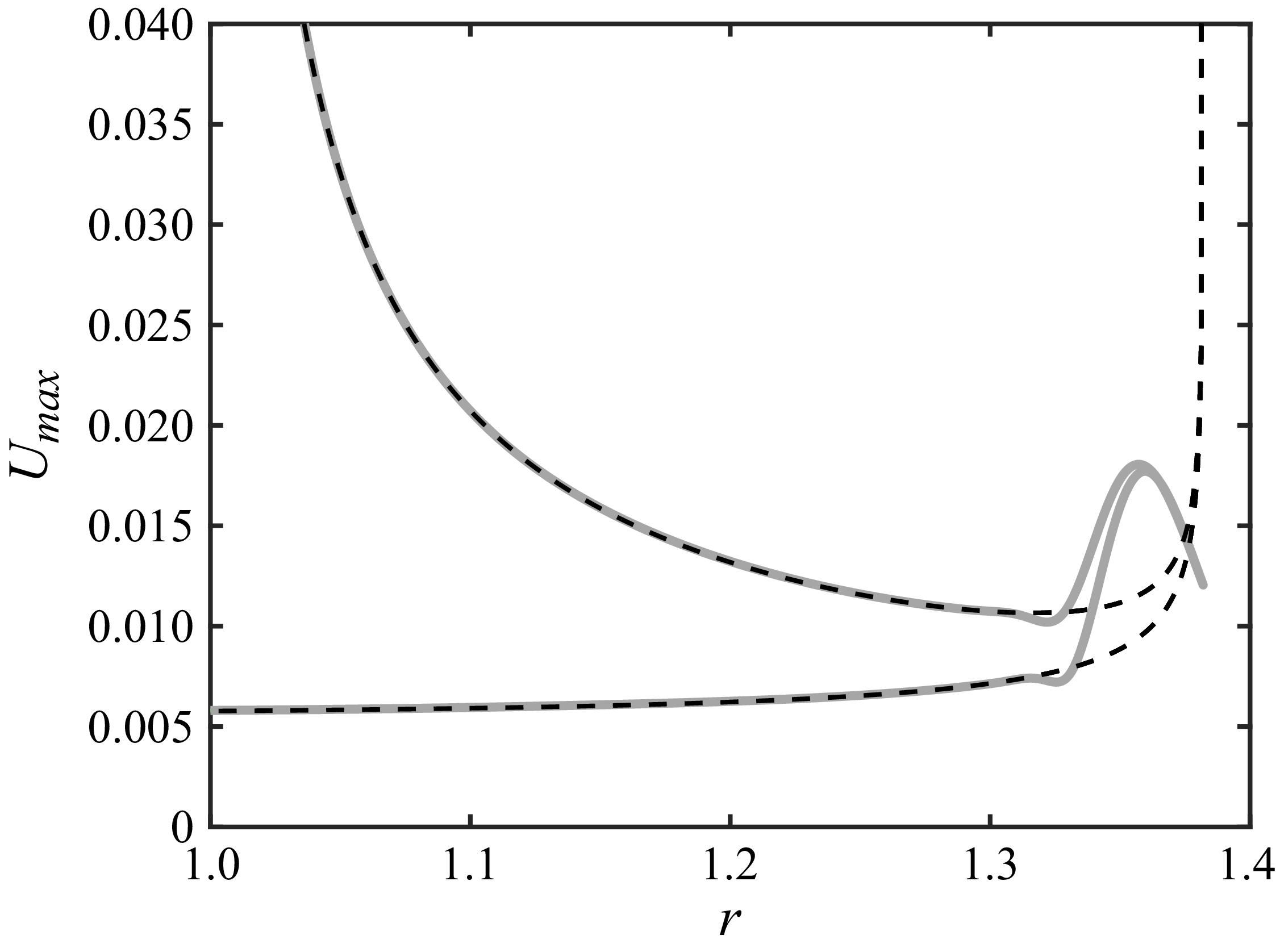


 Open access