


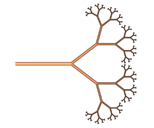



1. Introduction
Fluidic networks are ubiquitous in biological systems and engineering applications, as shown in figure 1(a). In biology, these networks are found in e.g. vascular networks (Murray Reference Murray1926b; Hutchins, Miner & Boitnott Reference Hutchins, Miner and Boitnott1976; Lee & Lee Reference Lee and Lee2010), bronchial trees of the lungs (Hooper Reference Hooper1977; Xu et al. Reference Xu, Sasmito, Li and Qiu2016a), and leaf veins of plants (McCulloh, Sperry & Adler Reference McCulloh, Sperry and Adler2003; Gleason et al. Reference Gleason, Blackman, Gleason, McCulloh, Ocheltree and Westoby2018). Here, evolution has resulted in fluidic networks that efficiently transport large amounts of heat or mass, with low dissipation during fluid transport and limited volumes (Bejan & Lorente Reference Bejan and Lorente2013). These characteristics are also desirable for three recent fluidic-based platforms: microfluidics (Whitesides Reference Whitesides2006), including microreactors (Dong et al. Reference Dong, Wen, Zhao, Kuhn and Noël2021), additive manufacturing (Visser et al. Reference Visser, Amato, Mueller and Lewis2019), and functional ‘Murray’ materials in which heat or mass is diffused through the channel walls to the surrounding material (Sciubba Reference Sciubba2016; Zheng et al. Reference Zheng, Shen, Wang, Li, Dunphy, Hasan, Brinker and Su2017). However, the per-channel throughput of these platforms is intrinsically low, for example because long reaction times are required in microreactors (Su et al. Reference Su, Kuijpers, Hessel and Noël2016; Madhawan et al. Reference Madhawan, Arora, Das, Kuila and Sharma2018). The per-channel flow rate of microfluidic systems can be increased by 1–3 orders of magnitude by entering the inertial regime (Di Carlo Reference Di Carlo2009) or by in-air microfluidics (Visser et al. Reference Visser, Kamperman, Karbaat, Lohse and Karperien2018), but even this is insufficient for large-scale use. Paralellisation of these technologies is therefore required to harvest their full benefit (Holtze Reference Holtze2013; Skylar-Scott et al. Reference Skylar-Scott, Mueller, Visser and Lewis2019; Dong et al. Reference Dong, Chen, Liu, Hounjet, Cao, Stoyanov, Yang and Zhang2022). For example, in microfluidics, Jeong et al. (Reference Jeong, Yelleswarapu, Yadavali, Issadore and Lee2015) achieved scaling of channels up to 1000 $\times$ to realise commercial throughput of particle-generating flows. In additive manufacturing of complex soft-robotic walkers, Skylar-Scott et al. (Reference Skylar-Scott, Mueller, Visser and Lewis2019) achieved direct-write via 128 parallel channels by repeated bifurcation from the main channel for the ‘ink’ supply. In materials science, reactors for heat or mass exchange were parallelised both top-down by Dong et al. (Reference Dong, Wen, Zhao, Kuhn and Noël2021) (resembling microfluidic chips) and bottom-up by self-assembly by Zheng et al. (Reference Zheng, Shen, Wang, Li, Dunphy, Hasan, Brinker and Su2017) (resembling biological materials). Upscaling by paralellisation is typically achieved by distributing flow to individual channels via branched fluidic networks. Figure 1(b) shows that several levels of fluidic branching were achieved for the aforementioned applications, but also that biological systems still exhibit a far larger number of branchings. Therefore, further optimisation of engineered networks may help in realising the enormous application potential of microfluidics, additive manufacturing, and Murray materials. Similarly, optimised fluidic networks would benefit upscaling of emerging methods for catalysis (Yi et al. Reference Yi, Lu, Wu, Wang and Luo2022), carbon capture (Moore et al. Reference Moore, Biviano, Mumford, Dagastine, Stevens and Webley2019), droplet and particle production (Holtze Reference Holtze2013; Yadavali, Jeong & Lee Reference Yadavali, Jeong and Lee2018), three-dimensional (3-D) printing of polymer foams (Visser et al. Reference Visser, Amato, Mueller and Lewis2019), artificial arterial networks (Kinstlinger & Miller Reference Kinstlinger and Miller2016), and microfluidic blood oxygenation (Dabaghi et al. Reference Dabaghi, Rochow, Saraei, Mahendran, Fusch, Chan, Brash, Fusch and Selvaganapathy2020). The purpose of this paper is to provide optimisation tools that are suitable for a broad range of fluid rheologies and readily applicable by scientists and engineers who design fluidic networks.
(a) Examples of branched fluidic networks in engineering applications and biological systems. (b) Radius of the channel  $R_i$ in the network as a function of the relative flow rate $Q_i/Q_0$ at level $i$ for the networks corresponding to the examples in (a). Every marker indicates a level in the branching. The error bars indicate the deviation from the marker (Singhal, Henderson & Horsfield Reference Singhal, Henderson and Horsfield1973; Gan et al. Reference Gan, Tian, Yen and Kassab1993; Kassab et al. Reference Kassab, Rider, Tang and Fung1993; Nordsletten et al. Reference Nordsletten, Blackett, Bentley, Ritman and Smith2006; Su et al. Reference Su, Kuijpers, Hessel and Noël2016; Carvalho et al. Reference Carvalho, Turgeon, Owens and Niklas2017; Zheng et al. Reference Zheng, Shen, Wang, Li, Dunphy, Hasan, Brinker and Su2017; Zhao et al. Reference Zhao, Cambié, Janse, Wieland, Kuijpers, Hessel, Debije and Noël2018; Skylar-Scott et al. Reference Skylar-Scott, Mueller, Visser and Lewis2019). Adapted with permission from Skylar-Scott et al. (Reference Skylar-Scott, Mueller, Visser and Lewis2019), copyright (2019) The Authors, published by Springer Nature; and adapted under terms of the CC-BY licence from Zheng et al. (Reference Zheng, Shen, Wang, Li, Dunphy, Hasan, Brinker and Su2017), copyright (2017) The Authors, published by Springer Nature.

Theoretical analyses of fluidic networks, including the present work, are usually constructed in two steps (Murray Reference Murray1926b).
First, an expression is derived for the radius of a channel such that power consumption is minimised for a given flow rate. The key idea is to consider not only the power needed to maintain the flow, i.e. the product of pressure drop and flow rate, but also to minimise the channel's volume by considering the costs introduced by the volume in the channels. For that, a cost factor  $\alpha$, representing the power per volume needed to maintain the fluid, is multiplied with the volume and included in the power function. For example, Murray (Reference Murray1926b) proposed the use of the metabolic energy to maintain blood in the body as a cost factor. For more details on the cost factor, see § 2.4.
Assuming a laminar flow of an incompressible Newtonian fluid in an artery of circular cross-section, the cube of the radius  $R$ is proportional to the flow rate $Q$ for a power-optimised channel:
 \begin{equation} \frac{R^3}{Q}= \text{const.}\end{equation}
 Second, the network is optimised by considering a bifurcation consisting of a parent channel (index ‘0’) and two daughter channels (indices ‘1’ and ‘2’) (Murray Reference Murray1926a), as shown schematically in figures 2(a)–2(c). Employing mass conservation and assuming incompressibility ( $Q_0=Q_1+Q_2$), the radii of the tubes must satisfy
 \begin{equation} R_0^3 = R_1^3 + R_2^3, \end{equation}
if (1.1) is satisfied in all channels.
(a) Branching of parent channel into  $N$ daughter channels. The location of the branching point $\boldsymbol {x}$ follows from the analysis and determines the lengths $L_i$ of the channels. The grey channels indicate that it is possible to have many channels that originate from the branching point. (b) Schematic of a single branch. (c) Schematic of velocity profile of fully developed laminar flow of non-yield-stress fluid in pipe. (d) Schematic of velocity profile of fully developed laminar flow of yield-stress fluid in pipe. (e) The fluid models as analysed in this work. The colours are consistent across (c–f). ( f) Different fluid models characterised by $n$ and $\phi$. For the characterisation of Casson-like fluids, see Appendix A.

Murray's theory for this flow regime has been analysed further by e.g. Murray (Reference Murray1926a,Reference Murrayb), Zamir (Reference Zamir1977), Sherman (Reference Sherman1981), Kamiya, Togawa & Yamamota (Reference Kamiya, Togawa and Yamamota1974), Stephenson et al. (Reference Stephenson, Patronis, Holland and Lockerby2015), Oka & Nakai (Reference Oka and Nakai1987) and Miguel & Rocha (Reference Miguel and Rocha2018), and verified experimentally by e.g. Rossitti & Löfgren (Reference Rossitti and Löfgren1993) and Hutchins et al. (Reference Hutchins, Miner and Boitnott1976). In addition, it has been extended to high turbulent flow of Newtonian fluids by Uylings (Reference Uylings1977), Kou et al. (Reference Kou, Chen, Zhou, Lu, Wu and Fan2014) and Stephenson & Lockerby (Reference Stephenson and Lockerby2016), and to laminar flow of non-Newtonian (power-law) fluids (Mayrovitz Reference Mayrovitz1987; Revellin et al. Reference Revellin, Rousset, Baud and Bonjour2009; Miguel & Rocha Reference Miguel and Rocha2018; Stephenson & Lockerby Reference Stephenson and Lockerby2016). Flow regimes of more complex fluid models – Bingham (Reiner Reference Reiner1926), Herschel–Bulkley (Herschel & Bulkley Reference Herschel and Bulkley1926) and Casson (Venkatesan et al. Reference Venkatesan, Sankar, Hemalatha and Yatim2013) – have been investigated for single pipe flow (Chhabra & Richardson Reference Chhabra and Richardson2008; Chilton & Stainsby Reference Chilton and Stainsby1998) (figure 2d). Ponalagusamy (Reference Ponalagusamy2012) explored optimal branching of fluidic networks containing yield-stress fluids (Bingham and Herschel–Bulkley). Next to channels with circular cross-sections, channels with elliptical (Tesch Reference Tesch2010) and rectangular (Emerson & Barber Reference Emerson and Barber2012) cross-sections have been introduced, from which it appeared that the cross-section does not affect Murray's proportionality, in contrast to the flow regime (i.e. laminar or turbulent), which can change Murray's cube rule. Other effects, such as the effect of curved channels (Miguel Reference Miguel2018), pulsating flow (Painter, Edén & Bengtsson Reference Painter, Edén and Bengtsson2006), asymmetric branching (Zamir Reference Zamir1978) and the efficiency difference between bifurcation and trifurcations (Rosenberg Reference Rosenberg2020), have been investigated. The state of the art is discussed in more detail in Revellin et al. (Reference Revellin, Rousset, Baud and Bonjour2009), Bejan & Lorente (Reference Bejan and Lorente2006), Miguel (Reference Miguel2016) and Xu et al. (Reference Xu, Sasmito, Yu and Mujumdar2016b).
Next to the radii of the channels, the location of the branching point  $\boldsymbol {x}$ is an important variable in the optimisation of the network, as it determines the lengths of the channels for a network with given end points $\boldsymbol {x}_i$, $i=0,1,\ldots,N$ (see figure 2a). Mostly, when theoretically optimising a fluidic network, this is done by Murray's proposal to minimise both the power of driving the fluid (minimisation of resistance) and the power to maintain the fluid (minimisation of volume) (Murray Reference Murray1926a,Reference Murrayb; Uylings Reference Uylings1977). Consequently, $\boldsymbol {x}$ has to be chosen such that the volume of the channels is minimal. The angles formed between the parent and daughter channels have gained special attention, and were investigated for the case of a bifurcation or a symmetric trifurcation, theoretically (Murray Reference Murray1926a; Horsfield & Cumming Reference Horsfield and Cumming1967; Kamiya & Togawa Reference Kamiya and Togawa1972; Uylings Reference Uylings1977; Zamir Reference Zamir1976, Reference Zamir1977) and experimentally (Hutchins et al. Reference Hutchins, Miner and Boitnott1976; Horsfield & Cumming Reference Horsfield and Cumming1967). These angles depend on the channel radii and the type of minimisation (Zamir Reference Zamir1976), and on other constraints such as fixed pressures at end points (Kamiya & Togawa Reference Kamiya and Togawa1972). Although the theoretical optimal radii of the channels match well with the observed results in biology, the correlation between theoretical optimal and observed angles between the channels is weaker (Hutchins et al. Reference Hutchins, Miner and Boitnott1976), possibly related to additional geometrical constraints beyond network optimisation (Horsfield & Cumming Reference Horsfield and Cumming1967; Hutchins et al. Reference Hutchins, Miner and Boitnott1976).
Despite all of the previous results, engineering branched fluidic networks remains challenging. First, many sources aim to describe biological fluidic networks, but biological networks are not only designed for energy minimisation (Koçillari Reference Koçillari2021) and current methods are less suitable for engineering purposes. Second, complex mathematical calculations are often required to optimise networks that transport non-Newtonian fluids (see e.g. Ponalagusamy Reference Ponalagusamy2012). Third, alternative fluid models such as Casson have not been applied in branched fluidic networks before, despite their applicability to e.g. food processing and blood.
Therefore, here we introduce a procedure for calculating the geometry of an optimal branching for fully developed laminar flow of simple and complex fluid models (figure 2e), which is described in § 2. The losses of non-optimised networks, the wall shear stress, the self-similar velocity profile, and approaches to determine the cost factor are discussed. Section 3 shows example cases of the optimisation method, after which the validity of the theory is discussed in § 4, and the conclusions are presented in § 5.
2. Optimisation of a branching using Murray's theory
We consider a branching consisting of a parent channel connected to  $N$ daughter channels in a branching point $\boldsymbol {x}$; see figure 2(a). The channels are numbered from $0$ to $N$, with $0$ indicating the parent channel. In this study, we choose to fix the flow rates $Q_i$, $i=0,1,\ldots,N$, and the position of the termination points of the channels $\boldsymbol {x}_i$, $i=0,1,\ldots,N$. These parameters being fixed, we aim at minimising the power required to perform this flow, with respect to the effective radii $R_i$, $i=0,1,\ldots,N$, of the channels and to the location of the branching point $\boldsymbol {x}$. Furthermore, $Q_0$ is taken positive towards the branching point, whereas the flow rates in the daughter channels $Q_i$, $i=1,\ldots,N$, are taken positive away from the branching point. To satisfy mass conservation (assuming incompressibility), the flow rates satisfy
 \begin{equation} Q_0=\sum_{i=1}^N Q_i. \end{equation}
The effective radius is defined as  $R\equiv D_H/2$, where $D_H \equiv 4A/p$ is the hydraulic diameter, with $A$ being the cross-sectional area of the channel, and $p$ being the wetted perimeter of the cross-section. This can be used for deriving the flow rate through elliptical and rectangular cross-sections, and comparing channel characteristics, but will result in different expressions for the flow rate $Q$ than for circular cross-sections. In the present study, the focus is on only circular cross-sections, and here, the effective radius reduces to the channel radius. For channel flow with elliptical and rectangular cross-sections, the reader is referred to e.g. Tesch (Reference Tesch2010), Emerson & Barber (Reference Emerson and Barber2012), Lekner (Reference Lekner2007) and Cornish (Reference Cornish1928).
Furthermore, the lengths of the channels  $L_i$ are functions of the branching location:
 \begin{equation} L_i\equiv|\boldsymbol{x}_i-\boldsymbol{x}|, \quad i=0,1,\ldots,N. \end{equation}
The power depends on the radii and lengths of the channels, and is the sum of the individual channel contributions:
 \begin{equation} P(\boldsymbol{R},\boldsymbol{x}) \equiv \sum_{i=0}^N \left\{\left|\frac{{\rm d}p}{{\rm d}z}\right| QL + \alpha V\right\}_i. \end{equation}
Here,  $V$ is the channel volume, with
 \begin{equation} V_i = {\rm \pi}R_i^2 L_i, \end{equation}
the pressure gradient  $|{\rm d}p/{\rm d}z|$ is a fluid-type dependent function derived in § 2.1, and $z$ is the coordinate in the flow direction of a channel. The pressure at the nodes is not defined or constrained. The cost factor is $\alpha$, representing the power per unit volume required to maintain the fluid ( $\alpha \approx 1\ {\rm kW}\ {\rm m}^{-3}$; Murray Reference Murray1926b).
Optimisation of the branched network is carried out by differentiation of (2.3) to  $\boldsymbol {R}$ and $\boldsymbol {x}$, and equating these expressions to 0. From this, one obtains optimisation problems for: (1) the channel radii $\boldsymbol {R}$ (§ 2.2), and (2) the location of the branching point $\boldsymbol {x}$ (§ 2.3). The flow profile, dissipation characteristics and wall shear stress of the branched network are discussed in § 2.4.
2.1. Fully developed laminar channel flow
The pressure difference needed to drive a fluid through a channel is governed by the ‘fluid model’ that describes the rheological behaviour of the fluid. The (effective) dynamic viscosity  $\mu$ describes the resistance of the fluid against shear, which can be shear-rate $\dot {\gamma }$ dependent according to $\mu = \mu '\,|\dot {\gamma }|^{n-1}$. Here, $\mu '$ is the flow consistency index, and $n>0$ is the flow index, with $n>1$ representing shear-thickening, and $0< n<1$ representing shear-thinning behaviour of the fluid. Furthermore, a fluid may have a yield stress $\tau _0 \geqslant 0$, which means that the fluid shears only if the local shear stress $\tau _{rz}$ exceeds the yield stress. The shear rate of the fluid as a function of the applied local shear stress for a Herschel–Bulkley fluid is described as
 \begin{equation} \dot{\gamma}(\tau_{rz}) = \begin{cases} \text{sign}(\tau_{rz})\left(\dfrac{|\tau_{rz}|-\tau_0}{\mu'} \right)^{1/n} & \text{if $|\tau_{rz}|\geqslant\tau_0$},\\[8pt] 0 & \text{if $|\tau_{rz}|<\tau_0$}. \end{cases} \end{equation}
Here,  $\dot {\gamma }\equiv {\partial u}/{\partial r}\leqslant 0$, with $u$ the axial velocity. The velocity in the radial and azimuthal directions is assumed to be 0. In the following, we assume that fluid properties $\mu '$, $\tau _0$ and $n$ are constant, and that there is fully developed laminar flow in cylindrical channels.
The local shear stress (with  $R\ll L$) is then described as a function of the axial pressure gradient ${\rm d}p/{\rm d}z$:
 \begin{equation} \tau_{rz} ={-}\frac{1}{2}\,\frac{{\rm d}p}{{\rm d}z}\,r, \end{equation}
with  $r$ the radial coordinate. Let $R$ be the radius of the channel, and let $R_p$ be the plug radius in case of yield-stress fluids:
 \begin{equation} R_p \equiv \frac{2\tau_0}{\left|\dfrac{{\rm d}{p}}{{\rm d}z}\right|}. \end{equation}
A schematic image of the plug radius  $R_p$ is presented in figure 2(d). Scaling this plug radius with the radius of the tube results in the dimensionless plug radius $\phi$:
 \begin{equation} \phi \equiv \frac{R_p}{R} = \frac{2\tau_0}{\left|\dfrac{{\rm d}{p}}{{\rm d}z}\right|R}. \end{equation}
Using these definitions, (2.5) can be rewritten in terms of  $\phi$ and $n$:
$n$:
 \begin{equation} \dot{\gamma}(r) = \begin{cases} \text{sign}(\tau_{rz})\left( \left(\dfrac{R}{2\mu'}\left|\dfrac{{\rm d}{p}}{{\rm d}z}\right|\right) \Bigg(\dfrac{r}{R}-\phi\Bigg)\right)^{1/n} & \text{if $r\geqslant R_p$},\\[12pt] 0 & \text{if $r< R_p$}. \end{cases} \end{equation}
Figure 2( f) gives an overview of the different values assigned to  $\phi$ and $n$ for each fluid model. For Newtonian fluids, (2.9) collapses to the well-known equation $\dot {\gamma }(r) = \text {sign}(\tau_{rz})\,({r}/{2\mu })\,|{\rm d}p/{\rm d}z|$. For a derivation of Casson-like fluids (such as blood), see Appendix A.
Integration of  $\dot {\gamma }$ and applying a no-slip boundary condition at the wall ( $u(r=R)=0$) results in the velocity profile
 \begin{align} u(r) = \begin{cases}
\dfrac{nR}{n+1}\left(\dfrac{R}{2\mu'}\left|\dfrac{{\rm
d}p}{{\rm d}z}\right|\right)^{1/n}
\Biggl((1-\phi)^{{(1+n)}/{n}} -
\Biggl(\dfrac{r}{R}-\phi\Biggr)^{({1+n})/{n}} \Biggr) &
\text{if $r\geqslant R_p$},\\[12pt]
\dfrac{nR}{n+1}\left(\dfrac{R}{2\mu'}\left|\dfrac{{\rm
d}p}{{\rm d}z}\right|\right)^{1/n} (1-\phi)^{({1+n})/{n}} &
\text{if $r< R_p$}. \end{cases}
\end{align}
\begin{align} u(r) = \begin{cases}
\dfrac{nR}{n+1}\left(\dfrac{R}{2\mu'}\left|\dfrac{{\rm
d}p}{{\rm d}z}\right|\right)^{1/n}
\Biggl((1-\phi)^{{(1+n)}/{n}} -
\Biggl(\dfrac{r}{R}-\phi\Biggr)^{({1+n})/{n}} \Biggr) &
\text{if $r\geqslant R_p$},\\[12pt]
\dfrac{nR}{n+1}\left(\dfrac{R}{2\mu'}\left|\dfrac{{\rm
d}p}{{\rm d}z}\right|\right)^{1/n} (1-\phi)^{({1+n})/{n}} &
\text{if $r< R_p$}. \end{cases}
\end{align}
Here,  $u$ is restricted to a velocity profile directed positively in the $z$ direction. The negative direction is simply $-u(r)$. The flow field is integrated over the cross-section to obtain the flow rate $Q$:
$Q$:
 \begin{equation} Q \equiv \iint_A u(r) \,\text{d}A = 2{\rm \pi} \int^R_0 u(r)\,r \,\text{d}r, \end{equation}
so  $Q$ is a function of $|{\rm d}p/{\rm d}z|$, $R$,
$R$,  $\mu '$, $\tau _0$ and $n$. Dimension analysis shows that $Q$ can be written in the form
 \begin{equation} Q = {\rm \pi}R^3 \left(\frac{R}{2\mu'}\left|\frac{{\rm d}p}{{\rm d}z}\right|\right)^{1/n} \left(\frac{n}{3n+1}\right)\times \psi(\phi,n), \end{equation}
or, in terms of  $\phi$ as
 \begin{equation} Q = {\rm \pi}R^3\left(\frac{\tau_0}{\mu'\phi}\right)^{1/n} \left(\frac{n}{3n+1}\right)\times \psi(\phi,n), \end{equation}
where we have included the factor  ${{\rm \pi} n}/({3n+1})$ for convenience. Here, $\psi (\phi,n)$ is the dimensionless flow rate – the ratio of the flow rate $Q$ and the flow rate of a non-yield fluid $Q_{NY}$ – which is dependent solely on $\phi$ and $n$, and has a value between 0 and 1. The pressure gradient in relation to the flow rate $Q$ is obtained by rewriting (2.12):
 \begin{equation} \left|\frac{{\rm d}p}{{\rm d}z}\right| = \frac{2\mu'}{R}\left(\frac{Q}{{\rm \pi} R^3}\right)^n \left(\frac{3n+1}{n}\right)^n\frac{1}{\psi(\phi,n)^n}. \end{equation}
 The general expression for  $\psi (\phi,n)$ can be found by computing the integral in (2.11):
 \begin{equation} \psi = \frac{(1-\phi)^{(n+1)/n}}{(3n+1)^{{-}1}} \times\left( \frac{(1-\phi)^2}{3n+1}+\frac{2\phi(1-\phi)}{2n+1}+\frac{\phi^2}{n+1}\right). \end{equation}
For Bingham fluids ( $n=1$), the expression for $\psi$ reduces to
 \begin{equation} \psi = 1-\tfrac{4}{3}\phi+\tfrac{1}{3}\phi^4 , \end{equation}
and for the case of non-yield-stress fluids ( $\phi =0$), $\psi$ always reduces to 1.
Equation (2.13) shows that  $Q/R^3$ is solely a function of the dimensionless plug radius $\phi$, and vice versa. The same holds for the term $|{\rm d}p/{\rm d}z|\,R$, which is obtained if $\phi$ is known. This property will be used in the characterisation of the optimised networks.
The Darcy–Weisbach equation is commonly used for calculation of the pressure drop for pipe flow, which is given as
 \begin{equation} \Delta p = f\,\frac{\rho}{4{\rm \pi}^2 }\,\frac{Q^2}{R^5}\,L, \end{equation}
in which the Darcy friction factor  $f$ for the laminar flows of all treated fluid models is then provided by
 \begin{equation} f = \frac{64}{Re'\,\psi^n}, \end{equation}
where (Garcia & Steffe Reference Garcia and Steffe1987)
 \begin{equation} Re' = 8\left(\frac{n}{3n+1}\right)^n\frac{\rho}{\mu'}\left(\frac{Q}{{\rm \pi} R^3}\right)^{2-n} R^2. \end{equation}
 For optimised fluidic networks with laminar flow in the first branch ( $R^3/Q = \text {const}.$, as discussed in the next subsection), $Re'$ scales with $R^2$, a generalisation of what Cohn (Reference Cohn1955) derived for symmetric bifurcations. Therefore, all daughter channels will have a lower Reynolds number than the parent channel, ensuring laminar flow throughout the network if $Re'_0< Re'_{crit}$. The critical Reynolds number $Re'_{crit}$ is a function of $\phi$ and $n$ that was derived to be (Hanks & Ricks Reference Hanks and Ricks1974):
 \begin{equation} Re'_{crit} =\frac{6464n}{(1+3n)^2}\times (2+n)^{({2+n})/({1+n})}\times\frac{\psi^{2-n}}{(1-\phi)^{({n+2})/{n}}}, \end{equation}
which reduces to  $Re'_{crit} \approx 2100$ for Newtonian fluids.
2.2. Optimisation of the channel radii
Every channel within a branching contributes to the total power. When differentiating the total power to the individual radii  $R_i$ for given flow rate $Q_i$, it is found that the optimisation condition for that radius $R_i$ depends only on the power contribution of the corresponding channel. Furthermore, the optimal radii $R_i$ do not depend on the lengths of the channels $L_i$. Therefore, calculation of the optimal channel radius is a decoupled problem, in which the power defined by (2.3) attains a global minimum with respect to the radius of each individual channel if
 \begin{equation} \frac{\partial P_i}{\partial R_i}=\frac{\partial}{\partial R_i}\left(\left|\frac{{\rm d}p}{{\rm d}z}\right|_i\right)Q_iL_i+2{\rm \pi}\alpha R_iL_i=0, \quad i=0,1,\ldots,N. \end{equation}
The optimisation condition for  $R_i$ is obtained by differentiating (2.14) to $R_i$ (see § B.1), resulting in
 \begin{equation} \frac{R_{i,*}^3}{Q_i} = \frac{1}{\rm \pi}\left(\frac{\mu'}{\alpha}\left(\frac{3n+1}{n}\right)^n\frac{J_*}{\psi_*^n}\right)^{1/(n+1)}, \quad i=0,1,\ldots,N, \end{equation}
where functions evaluated at optimal radius are denoted by a subscript  $*$, and $J$ is defined as
 \begin{equation} J\equiv 1+\frac{3n}{1-\dfrac{n\phi}{\psi}\,\dfrac{\partial \psi}{\partial\phi}}. \end{equation}
For a Herschel–Bulkley fluid, substitution of  $\psi$ from (2.15) into (2.23) results in the expression
 \begin{equation} J = \frac{3n+1}{\dfrac{6n^3}{(2n+1)(n+1)}\,\phi^3+\dfrac{6n^2}{(2n+1)(n+1)}\,\phi^2+\dfrac{3n}{2n+1}\,\phi +1}. \end{equation}
For Bingham fluids ( $n=1$), the expression for $J$ reduces further to
 \begin{equation} J = \frac{4}{\phi^3+\phi^2+\phi +1}, \end{equation}
and for non-yield fluids ( $\phi =0$), it reduces to $J=3n+1$. Finally, for $\phi =1$, one obtains $J=1$.
For the case of Newtonian and power-law fluids ( $\phi =0$), the optimisation condition for $R_*^3/Q$ is calculated relatively easily (with $J_*=3n+1$ and $\psi _*=1$). However, for yield-stress fluids, determining the optimal value for $R_*^3/Q$ is more difficult. Therefore, the following procedure is proposed.
First, the following dimensionless numbers are introduced:
 $$\begin{gather} \frac{\tilde{R}^3}{\tilde{Q}}\equiv \frac{R^3}{Q}\left(\frac{\alpha}{\mu'}\right)^{{1}/({n+1})}, \end{gather}$$
 $$\begin{gather}\tilde{\tau}_0 \equiv \frac{\tau_0}{(\mu'\alpha^n)^{{1}/({n+1})}}. \end{gather}$$
Using these dimensionless numbers, (2.22) is rewritten as
 \begin{equation} \frac{\tilde{R}_{i,*}^3}{\tilde{Q_i}} = \frac{1}{\rm \pi}\left(\left(\frac{3n+1}{n}\right)^n\frac{J_*}{\psi_*^n}\right)^{1/(n+1)}, \quad i=0,1,\ldots,N. \end{equation}
Applying the same non-dimensionalisation to (2.13), and rewriting it as a function of  $\psi$, then substitution into (2.28), results in the alternative expression
 \begin{equation} \frac{\tilde{R}_{i,*}^3}{\tilde{Q_i}} = \frac{J_*\tilde{\tau}_{0}}{{\rm \pi}\phi_*}, \quad i=0,1,\ldots,N. \end{equation}
When eliminating  $\tilde {R}_*^3/\tilde {Q}$ from (2.28) and (2.29), we obtain the expression
 \begin{equation} \tilde{\tau}_{0} = \phi_* \left(\frac{3n+1}{n\,J_*(\phi_*,n)\,\psi_*(\phi_*,n)}\right)^{{n}/({n+1})}. \end{equation}
Here,  $\tilde {\tau }_0$ is composed of fluid and system properties, and is therefore considered as known for an optimisation process. As both $\psi$ and $J$ are solely functions of $\phi$ and $n$, the value of $\phi _*$ corresponding to $\tilde {\tau }_{0}$ can be found implicitly using (2.15) and (2.24). Figure 3 shows the calculated optimal values of $\phi _*$ as functions of $\tilde {\tau }_0$ and $n$. Using $\phi _*$, the corresponding optimisation condition for $\tilde {R}_{i,*}^3/\tilde {Q}_i$ is calculated readily using (2.28) or (2.29), and plotted in figure 4. The optimal channel diameter $R_{i,*}$ at desired flow rate $Q_i$ then follows directly from (2.26).
Contour plot of the dimensionless plug radius for the optimised network  $\phi _*$ as a function of $\tilde {\tau }_{0}$ and $n$.
$n$.

Contour plot of  $\tilde {R}_*^3/\tilde {Q}$ as a function of $\tilde {\tau }_0$ and $n$. The colours represent the different fluid models and correspond to figure 2. The Herschel–Bulkley model covers the entire parameter space of $\tilde {\tau }_0$ and $n$.
$n$.

For the non-yield limit ( $\tilde {\tau }_0\rightarrow 0$), the optimisation condition becomes $\tilde {R}_{i,*}^3/\tilde{Q_i}\approx ({3n+1}){{\rm \pi} }^{-1}\, n^{(-n/(n+1))}$, which has a maximum $\tilde {R}_{i,*}^3/\tilde{Q_i}\approx 1.41$. This simplified expression is valid for $\tilde {\tau }_0<10^{-2}$, because then the fluid yield-stress effect in the optimised network becomes negligible. For larger values of $\tilde {\tau }_0$, plug formation becomes more relevant, and $\tilde {R}_{i,*}^3/\tilde{Q_i}$ becomes larger than in the case of a non-yield fluid. For the yield limit ( $\tilde {\tau }_0\rightarrow \infty$), the optimisation condition tends to go to $\tilde {R}_{i,*}^3/\tilde{Q_i}\rightarrow \tilde {\tau }_0/{\rm \pi}$. Figure 4 also shows the parameter space of the different fluid models. The graphical approach of figure 4 for the optimal value of $R_{i,*}^3/Q_i$ for complex fluids prevents extensive calculations, enabling straightforward optimisation of the geometry of fluidic networks.
2.3. Optimisation of the network topology
When the optimal channel radii are calculated according to § 2.2, the second optimisation step is made to provide the location of the branching point  $\boldsymbol {x}$. As shown in figure 2(a), the location of the branching point determines the length of all channels. Therefore, the optimised branching point $\boldsymbol {x}_*$ minimises the total (volume- and dissipation-induced) power of the network. Now the total power consumption of the network in (2.3) is differentiated to $\boldsymbol {x}$ and set to 0, resulting in
 \begin{equation} \boldsymbol{\nabla}_{\boldsymbol{x}}{P}=\sum_{i=0}^N\left(\left|\frac{{\rm d}p}{{\rm d}z}\right|_i Q_i + \alpha{\rm \pi} R_i^2\right) \boldsymbol{\nabla} L_i=0. \end{equation}
Substituting the optimal radii (2.22) results in the optimisation condition of the branching point  $\boldsymbol {x}=\boldsymbol {x}_*$ (for a full derivation, see § B.2):
 \begin{equation} \sum_{i=0}^N R_{i,*}^2 \boldsymbol{e}_{i,*}=\textbf{0}, \quad \boldsymbol{e}_{i,*}\equiv\left(\boldsymbol{\nabla} L_i\right)_*=\frac{\boldsymbol{x}_*-\boldsymbol{x}_i}{|\boldsymbol{x}_*-\boldsymbol{x}_i|}. \end{equation}
From this implicit equation, the coordinates of  $\boldsymbol {x}_*$ are solved by simple numerical methods, providing $V_i$. Note that $\boldsymbol {x}_*$ can be located in a 3-D space, depending on the location of the end points $\boldsymbol {x}_i$. The resulting $\boldsymbol {x}_*$ determines a network that is optimised with respect to both the channel radii (2.22) and the channel lengths (2.32a,b).
The global minimum power of the branched network  $P$ is obtained by inserting the result of (2.22) into (2.3):
 \begin{equation} P_*=\left(\frac{J_*+2}{J_*}\right)\alpha \sum_{i=0}^N V_{i,*}. \end{equation}
 The angles between the channels are calculated by taking the inner product of (2.32a,b) with unit vectors that originate in the branching point and point towards the nodes. The resulting cosines of the corresponding angles between the two unit vectors can be calculated using  $\cos (\theta _{ij})=\boldsymbol {e}_i\boldsymbol {\cdot }\boldsymbol {e}_j$:
 \begin{equation} \sum_{i=0}^N R_{i,*}^2 \boldsymbol{e}_{i,*}\boldsymbol{\cdot} \boldsymbol{e}_{j,*}=0. \end{equation}
This equation results in a linear system of  $N+1$ equations for $\boldsymbol {e}_{i}\boldsymbol {\cdot } \boldsymbol {e}_{j}$ ( $i,j=0,1,\ldots,N$, with $i\neq j$). For a bifurcation and a symmetric trifurcation, the angles between the channels for the optimal branching are independent of the coordinates of the nodes $\boldsymbol {x}_i$ (see figure 5). For both symmetric and asymmetric bifurcations, i.e. $N=2$, the optimal branching point $\boldsymbol {x}_*$ lies in a plane in the 3-D space spanned by $\boldsymbol {x}_0,\boldsymbol {x}_1,\boldsymbol {x}_2$, as shown in figure 5(a). The cosines of the smallest angles between each pair of channels involved are given by
 \begin{equation} \left.\begin{gathered} \boldsymbol{e}_0\boldsymbol{\cdot}\boldsymbol{e}_1=\cos(\theta_{01})={-}\frac{R_0^4+R_1^4-R_2^4}{2R_0^2R_1^2}, \\ \boldsymbol{e}_0\boldsymbol{\cdot}\boldsymbol{e}_2=\cos(\theta_{02})={-}\frac{R_0^4-R_1^4+R_2^4}{2R_0^2R_2^2}, \\ \boldsymbol{e}_1\boldsymbol{\cdot}\boldsymbol{e}_2=\cos(\theta_{12})=\frac{R_0^4-R_1^4-R_2^4}{2R_1^2R_2^2}. \end{gathered}\right\} \end{equation}
(a) Angles  $\theta _{ij}$ in a bifurcation. (b) Angles $\theta _{ij}$ in a trifurcation

For a symmetric trifurcation, i.e.  $N=3$, the optimal branching point $\boldsymbol {x}_*$ lies in a plane in the 3-D space spanned by $\boldsymbol {x}_0$, $\boldsymbol {x}_1$ or $\boldsymbol {x}_3$, and $\boldsymbol {x}_2$, where symmetry is assumed, i.e. channels 1 and 3 are mirrored in the line from $\boldsymbol {x}_0$ to $\boldsymbol {x}_2$ (figure 5b). This means that $R_1=R_3$, and the angles that they make with channels 0 and 2 are equal. In addition, $\boldsymbol {x}_0$, $\boldsymbol {x}_*$ and $\boldsymbol {x}_2$ are on the same line, reducing the unknown angles even further. The cosines of the smallest angles between each pair of channels involved are given by
 \begin{equation} \left.\begin{gathered} \boldsymbol{e}_0\boldsymbol{\cdot}\boldsymbol{e}_1=\frac{R_2^2-R_0^2}{2R_1^2}, \\ \boldsymbol{e}_1\boldsymbol{\cdot}\boldsymbol{e}_2=\frac{R_0^2-R_2^2}{2R_1^2}, \\ \boldsymbol{e}_1\boldsymbol{\cdot}\boldsymbol{e}_3=\frac{(R_0^2-R_2^2)^2-2R_1^4}{2R_1^4}. \end{gathered}\right\}\end{equation}
The results in (2.35) and (2.36) are in line with the findings of e.g. Zamir (Reference Zamir1976).
For other cases, the coordinates of  $\boldsymbol {x}_i$ are needed for calculating the angles between the channels because the system of equations from (2.34) is underdetermined. For a derivation of this general case as well as the above equations for bifurcations and trifurcations, see Appendix C.
2.4. The effect of non-optimised branching, the velocity profile, the wall shear stress, and the cost factor
Existing fluidic networks are not always optimised, as their dimensions may depend on physical constraints or industry standards. In this subsection, we compare the energy dissipation of such non-ideal networks to optimised fluidic networks as described in §§ 2.2 and 2.3.
For single channels within a network, the minimum power for a channel optimised with respect to the channel radius is obtained by taking the  $i$th element of (2.3) and substituting (2.14) and the optimisation condition (2.22):
 \begin{equation} P_{i,*} = \frac{J_*+2}{J_*}\,\alpha {\rm \pi}R_{i,*}^2 L_i, \quad i=0,1,\ldots,N. \end{equation}
 Next, the ratio of the non-optimised power  $P_i$ and its minimum value $P_{i,*}$ per channel is found by dividing the $i$th element of (2.3) by (2.37) (see also § B.1):
 \begin{equation} \frac{P_i}{P_{i,*}} = \frac{2}{J_{*}+2}\left(\frac{\psi_{*}}{\psi_i}\right)^n \left(\frac{R_i}{R_{i,*}}\right)^{-(3n+1)} + \frac{J_{*}}{J_{*}+2}\left(\frac{R_i}{R_{i,*}}\right)^{2}, \quad i=0,1,\ldots,N. \end{equation}
Note that the optimal parameters  $J_*$, $\phi _*$ and $\psi _*$ are without index $i$, because these are constant over the whole optimised branching (see also below). Substitution of the optimal values for a certain fluid and system ( $J_*$ and $R_*$) results in an expression dependent on $\phi$ and $R$. As $\phi$ and $R$ are related by (2.13), the dimensionless power consumption is calculated by knowing the actual radii.
Substitution of  $\psi _*=\psi =1$ and $J_*=4$ for laminar flow of a Newtonian fluid in (2.38) recovers the relations for power dissipation in a network as obtained by Murray (Reference Murray1926b) and Uylings (Reference Uylings1977). The proof of this result is provided in § B.1.
The ratio of the actual power for the whole network  $P$ and the optimal power $P_*$ is given by
 \begin{equation} \frac{P}{P_*} = \sum_{i=0}^N \frac{P_i}{P_*} = \sum_{i=0}^N \frac{P_i}{P_{i,*}}\,\frac{P_{i,*}}{P_*}, \end{equation}
where
 \begin{equation} \frac{P_{i,*}}{P_*} = \frac{R_{i,*}^2L_{i,*}}{\sum_{i=0}^N R_{i,*}^2L_{i,*}}, \quad i=0,1,\ldots,N, \end{equation}
and  $P_{i}/P_{i,*}$ given by (2.38) is represented graphically in figure 6 as a function of $R_i/R_{i,*}$ and $\tilde {\tau }_0$, for several values of $n$. Choosing radii that are only 0.3 times smaller than optimal can result in orders of magnitude higher power consumption in comparison to optimised networks (especially for $n=1.5$ and fluids with a low yield stress). Section 3 provides an example of how figure 6 can be used to determine the power consumption of a fluidic network.
Contour plots of the power consumption of a channel, relative to the power of an optimal channel  $P_i/P_{i,*}$ (2.38) as functions of $R_i/R_{i,*}$ and $\tilde {\tau }_0$ for $n=0.5$, $n=1.0$ and $n=1.5$.

When the channel radii are non-ideal, this affects the location of the optimal branching point. In that case, one solves the following equation instead of (2.32a,b):
 \begin{equation} \sum_{i=0}^N \Bigg( \frac{2}{J_{*}} \left(\frac{R_i}{R_{i,*}}\right)^{-(3n+1)} \left(\frac{\psi_{*}}{\psi_i}\right)^n+ \left(\frac{R_i}{R_{i,*}}\right)^{2}\Bigg)R_{i,*}^2\boldsymbol{e}_{i,*}=\textbf{0}. \end{equation}
When  $R_i=R_{i,*}$, (2.41) reduces to (2.32a,b). For a derivation, see § B.2.
Equation (2.10) suggests a self-similar velocity profile, as it scales only with  $R$ and has the same shape in every optimised channel due to the constant $|\textrm {d}{p}/{\textrm {d}z}|\,R$ and $\phi$. To assess this property, we combine (2.22) into (2.13) to show that $R_{i,*}^{3}/Q_i = \textrm {const.}$ holds for every channel within an optimised branching for all treated fluid rheologies, in the following manner. Substitution of (2.22) into (2.13) gives an equation containing only constant fluid properties and $\phi$. Consequently, $\phi$ is constant for an optimised branching, and this is also a proof that $R^3/Q$ is constant in every channel of the branching. As $\phi$ is constant, $\psi$ and $|\textrm {d}p/{\textrm {d}z}|\,R$ are also constant in every channel. As a result of these invariants, the velocity profiles in the channels of an optimised branching are self-similar.
Furthermore, the wall shear stress averaged over the perimeter  $\langle \tau _w \rangle$ is a function of the fluid properties and the terms $R^3/Q$ and $\psi (\phi )$. As a result, the average wall shear stress is constant over the whole branching for laminar flow of all treated fluid models when the branching is optimised by (2.22):
 \begin{equation} \langle \tau_w \rangle \sim \left(\frac{Q}{R^{3}}\right)^n\frac{\mu'}{\psi^n}. \end{equation}
For the derivation, see Appendix D.
An estimate of the cost factor based on governing costs should be made per situation. One approach is similar to Murray's metabolic cost factor, based on the energy needed to maintain a fluid (such as maintenance of the blood or maintenance of a temperature by heating). Also, as elaborated in the second example in § 3, one could think of a print nozzle network filled with expensive ink, where costs are based on the electricity and material costs. Other cost factors have been described for plants, where the conduit wall volume determines the costs, as the wall should be strong enough to withstand the negative internal pressure (McCulloh et al. Reference McCulloh, Sperry and Adler2003), diffusive systems (Zheng et al. Reference Zheng, Shen, Wang, Li, Dunphy, Hasan, Brinker and Su2017), and systems that require drag minimisation (Woldenberg & Horsfield Reference Woldenberg and Horsfield1986).
Even if a cost factor  $\alpha$ is not known explicitly, it is possible to design an optimised network based on other constraints – for example, in 3-D printing, where a flow rate and a nozzle radius at an outlet are specified and are assumed to be optimal. A second approach is making a channel to require a certain average flow velocity or dimensionless number such as the Weber number, which serves as a relation to obtain the corresponding optimal $R$ for given $Q$. For both approaches, the ratio $R^3/Q$ is then known, and based on (2.22), the whole optimal network can be calculated. The cost factor can be made explicit by calculating the optimal $\phi$ from (2.13) and calculating $\alpha$ from (2.22).
3. Examples: optimisation of a branched fluidic network
This first example shows the convenience of the graphical approach in determination of  $R^3/Q$. Here, a branched fluidic network inspired on a lubrication system is optimised, which has a laminar flow of grease described by the Bingham model ( $\rho =1000\ \textrm {kg}\ \textrm {m}^{-3}$, $\mu '=1.85\ \textrm {Pa}\ \textrm {s}$, $n=1$, $\tau _0=1.0$ Pa), inspired by Westerberg et al. (Reference Westerberg, Lundström, Höglund and Lugt2010). The temperature of the lubricant is maintained by adding heat, resulting in a cost factor $\alpha = 100\ \textrm {W}\ \textrm {m}^{-3}$. The network has one parent channel (channel 0) and two daughter channels (channels 1 and 2, $N=2$). The nodes are given by $\boldsymbol {x}_0 = (0,0)$ m, $\boldsymbol {x}_1 = (0.0625,0.025)$ m, and $\boldsymbol {x}_2 = (0.0625,-0.025)$ m. The flow rate in the parent channel is $Q_0=10\ \textrm {ml}\ \min ^{-1}$, and the flow rates in the daughter channels are determined to be $Q_1 =Q_2= \frac {1}{2}Q_0$, so the bifurcation is symmetric.
The dimensionless yield stress  $\tilde {\tau }_0$ is calculated as $\tilde {\tau }_0=\tau _0/(\mu '\alpha ^n)^{1/(n+1)}$ = 0.074, after which the corresponding optimisation condition $R^3/Q \approx 1.29$ is easily read from figure 4. Alternatively, the optimal value of $\phi$ is calculated from (2.16), (2.25) and (2.30), resulting in $\phi _*=0.068$. With $\phi _*$, the corresponding optimal value for $\psi$ can be calculated using (2.15): $\psi _*=0.910$. With these parameters, (2.28) provides an analytic value for $\tilde {R}^3/\tilde {Q}$, being equal to 1.2889, which is readily rewritten to real units using (2.26), where $(\mu '/\alpha )^{1/(n+1)} = 0.136$ s: we obtain $R^3/Q=0.175$ s. Based on this condition, the main channel radius is calculated to be $R_0 = 3.08$ mm. Knowing that $R^3/Q$ must be constant, based on (2.22), the radii of the daughter channels are determined:
 \begin{equation} R_1=R_2= R_0 \left(\frac{Q_1}{Q_0}\right)^{{1}/{3}}=0.794 R_0 = 2.45\ \text{mm}. \end{equation}
 As a check on whether the flow is still laminar, the largest Reynolds number and critical Reynolds number in the network are calculated from (2.19) and (2.20):  $Re' = 0.0186$ and $Re'_{crit}=2357$, respectively. This shows that the flow in the whole network will stay laminar.
From (2.32a,b), it is calculated that the branching point is located at  $\boldsymbol {x}_*= (0.030,0.000)$ m. The resulting topology is visualised in figure 7(a), where we make use of the velocity profile given in (2.10). The angles between the channels for this optimised network are calculated using (2.34) and also shown in the figure.
Topology of branching with lubrication flow with  $N=2$ daughter channels. (a) Symmetric bifurcation. (b) Asymmetric bifurcation with $Q_1 = \frac {1}{3}Q_0$ and $Q_2 = \frac {2}{3}Q_0$.

To show the effect of an asymmetric flow rate division, the same example is taken, but now with flow rates  $Q_1 = \frac {1}{3}Q_0$ and $Q_2 = \frac {2}{3}Q_0$. In addition, the end points are chosen to be $\boldsymbol {x}_0 = (0,0)$ m, $\boldsymbol {x}_1 = (0.053,0.017)$ m and $\boldsymbol {x}_2 = (0.0625,-0.025)$ m. Then the optimisation condition $R^3/Q$ is the same as before, but the daughter channel radii are different. These are $R_1 = R_0(Q_1/Q_0)^{1/3} = 2.14$ mm and $R_2 = R_0(Q_2/Q_0)^{1/3} = 2.69$ mm. As a consequence, the location of the branching point and the corresponding angles between the channels become different. The angles are calculated using (2.34), and the topology is shown in figure 7(b). Here, one sees that the angle between the parent channel and the largest daughter channel has become larger, tending more to the limit of $180^\circ$.
In a second example, we optimise the channel radius of a hypothetical branching nozzle, as for example used in parallel direct-write (Skylar-Scott et al. Reference Skylar-Scott, Mueller, Visser and Lewis2019; see figure 1). A model fluid is described by the Herschel–Bulkley model ( $\rho = 1200\ \textrm {kg}\ \textrm {m}^{-3}$, $\mu '= 15\ \textrm {Pa}\ \textrm {s}^n$, $n=0.4$, $\tau _0=2000$ Pa). The cost factor is estimated to be the ratio of the material costs per volume and the electricity costs to pump the fluid for a certain operation time: $\alpha = {c\rho }/{E\,\Delta t}$. The fluid costs
  , electricity costs
  , and a print session takes $\Delta t = 18$ min. Then the cost factor is estimated at $\alpha = 1\ \textrm {GW}\ \textrm {m}^{-3}$. The flow rate of the parent channel is $Q_0 = 10\ \textrm {ml}\ \min ^{-1}$, and the channel splits up into $K=4$ levels of symmetric bifurcations. Calculating $\tilde {\tau }_0=\tau _0/(\mu '\alpha ^n)^{1/(n+1)}=0.78$ and using figure 4, we obtain a value for the optimisation condition as $\tilde {R}_{i,*}^3/\tilde {Q}_i \approx 1.14$. Therefore, the optimisation condition in real units becomes $R_{i,*}^3/Q_i = \tilde {R}_{i,*}^3/\tilde {Q}_i (\mu '/\alpha )^{1/(n+1)} = 2.9\times 10^{-6}$ s. Consequently, the optimal channel radii for the four different levels (where due to symmetry, every channel at the same level has the same size) are $R_0 = 79\ \mathrm {\mu } \textrm {m}$, $R_1 = 62\ \mathrm {\mu } \textrm {m}$, $R_2 = 50\ \mathrm {\mu } \textrm {m}$ and $R_3 = 39\ \mathrm {\mu } \textrm {m}$. These channels are unrealistically small, because their manufacture is challenging and the material cost within the channels may be small compared to e.g. depreciation of equipment. However, this example shows clearly how expensive fluids could drive miniaturisation of the system.
In a third example, we investigate how a microfluidic branched network with equally sized channels performs in comparison to an optimised network, for symmetric bifurcations and  $K=5$ levels. The fluid in the network is described by the Herschel–Bulkley model ( $n=0.5$, $\tau _0=1000$ Pa, $\mu '=200\ \textrm {Pa}\ \textrm {s}^n$; Skylar-Scott et al. Reference Skylar-Scott, Mueller, Visser and Lewis2019). The radius and flow rate of the channel were considered to be optimal for the channels at outlet and have values $R_{opt} = 250\ \mathrm {\mu } \textrm {m}$ and $Q_{opt} = 2\ \textrm {ml}\ \min ^{-1}$. Consequently, all channels have radius $250 \ \mathrm {\mu } \textrm {m}$, and the main parent channel has flow rate $Q_0=32\ \textrm {ml}\ \min ^{-1}$. The flow rate in the other channels is calculated according to equal distribution of $Q_0$. Furthermore, the channel lengths are assumed to be a function of the flow rate: $L_i/L_0 = (Q_i/Q_0)^{2/3}$. The optimisation condition based on the optimal channel becomes $R_{i,*}^3/Q_i = 4.69$ s. From that, the optimal radii are calculated, based on the known flow rate in each channel. Together with the optimisation condition $R_{i,*}^3/Q_i$, one can calculate the properties of the optimal network. Based on the optimal channel, one can calculate $\phi _*=0.14$ and $\psi _*=0.68$ using (2.13), which also yields $J_*=2.24$ using (2.24) and $\tilde {\tau }_{0,*}=0.210$ using (2.30). Calculation of the radius ratio $R_i/R_{i,*}$ for each channel provides the needed input for the power ratio per channel via (2.38) or figure 6. Multiplying each power ratio with the corresponding term $P_{i,*}/P_*$ from (2.40), and summing everything, results in the overall network power ratio $P/P_*= 2.38$. This shows that application of the optimal radii instead of equally sized channels could reduce 58 % of the power consumption in the network.
4. Discussion
The optimal geometry derived above does not incorporate the constraint that the pressure at all end points must be equal. Therefore, flow rates may deviate from the calculated flows for open-ended systems such as nozzles that exit into the air. This issue can be mitigated in general by a pressure control system at the end of every node. Fortunately, however, bifurcating channels that are symmetric with respect to both the flow rate and the geometry always exhibit the same pressure drop, and will therefore provide optimal flow through the network without active control. In addition, this problem is prevented for radius-wise optimised networks by requiring  $\sum _i L_i/R_i = \textrm {const.}$ for both branches that originate from a branching point.
Furthermore, Murray's theory (§§ 2.2 and 2.3) is sometimes simplified to the so-called Murray law stating that the cubed parent channel radius is equal to the sum of the cubed daughter channel radii (see e.g. Sherman Reference Sherman1981; Stephenson et al. Reference Stephenson, Patronis, Holland and Lockerby2015):
 \begin{equation} R_{0}^3=\sum_{i=1}^N R_{i}^3. \end{equation}
This relation is obtained by substituting  $Q_i$ from the optimisation condition (2.22) into the mass conservation equation (2.1), where the right-hand side of (2.22) is constant for an optimised network. It is important to note that a branching optimised by (2.22) automatically fulfils (4.1), but satisfying (4.1) does not necessarily give the optimal branching. This was already pointed out by Kamiya et al. (Reference Kamiya, Togawa and Yamamota1974). Rosenberg (Reference Rosenberg2020) analysed this point critically, and invalidated the conclusion by Sherman (Reference Sherman1981) that conservation of the cube of the radii in a branching point is the determinant condition for network optimisation for both symmetric and asymmetric branches, for whatever number of daughter channels. Therefore, (4.1) is not sufficient for determining the optimal radii, except for branchings in which the flow rate in all daughter channels is the same (e.g. symmetric bifurcations). In that case, (4.1) reduces to
 \begin{equation} \frac{R_i}{R_0}=N^{-{1}/{3}}, \quad i=1,2,\ldots,N. \end{equation}
 Finally, flow effects such as entrance effects, non-axisymmetric velocity profiles at junctions, and channel curvature effects have not been taken into account due to the assumption of the channel flows being fully developed. However, if the slenderness condition in the channels is satisfied ( $R\ll L$), then the major part of the flow is still governed by the fully developed flow equations. Therefore, the theorem is suitable for overall network design or as an analysis tool, but for design details near junctions, simulations or experiments are recommended.
5. Conclusions and outlook
A generalised approach to minimise power consumption of branched fluidic networks was developed for Newtonian, power-law, Bingham, Herschel–Bulkley and Casson-like fluids in the steady laminar regime.
First, the flow rate in a single channel was analysed, providing the pressure drop over a channel as a function of the fluid model and channel dimensions. Subsequently, the optimal network geometry was obtained by minimising power with respect to the channel radii and the location of the branching point. For all treated fluid rheologies, Murray's optimisation condition for all channels within a network was recovered:
 \begin{equation} \frac{\tilde{R}_{i,{*}}^{3}}{\tilde{Q}_i}=\mbox{const.,} \quad i=0,1,2,\ldots,N. \end{equation}
The value of this constant is represented graphically in figure 4, enabling optimisation of fluid networks for non-Newtonian systems with a minimum of mathematical analysis for the first time. Detailed analysis of the network provided the following additional results.
(i) Insight into the increase of power consumption in case of non-optimal channel radii, revealing potentially large energy gains.
(ii) A self-similar velocity profile across the network, resulting in a constant wall shear stress.
(iii) Multiple methods to estimate the cost factor to maintain the liquid flow.
(iv) Conditions for which optimal flow is maintained without active control of the pressure at every junction.
(v) Proof that if the parent channel is laminar, the entire optimised network exhibits laminar flow. The Darcy friction factor is provided.
Future work may further address situation-specific cost factors for engineering systems (Woldenberg & Horsfield Reference Woldenberg and Horsfield1986), as well as systems with a transition from turbulent to laminar flow regimes.
Acknowledgements
A. Smink is acknowledged for making images as part of figure 1(a).
Funding
This research was financially supported by the ‘Crazy Research’ grant of the Engineering Technology faculty of the University of Twente (Design and manufacturing of multifunctional porous networks).
Declaration of interests
The authors report no conflict of interest.
Author contributions
C.W.V. and R.H. had a shared coordinating role.
Appendix A. Derivation of channel flow and optimal branching for Casson-like fluids
In § 2.1, the fluid models for Newtonian, power-law, Bingham and Herschel–Bulkley fluids were presented, where the first three models are simplifications of the Herschel–Bulkley fluid model. For food processing and blood flows, another fluid model, the so-called ‘Casson’ model, is used (Venkatesan et al. Reference Venkatesan, Sankar, Hemalatha and Yatim2013; Chhabra & Richardson Reference Chhabra and Richardson2008). For large shear rates  $\dot {\gamma }$, the behaviour of the Casson model is similar to Bingham fluids, but especially for small $\dot {\gamma }$, the Casson model has a more gradual increase in shear stress with increasing shear rate, which describes the mentioned applications better. This gradual behaviour is accomplished by weighting the square roots of the terms in the fluid model, which is slightly more sophisticated than for Bingham and Herschel–Bulkley.
In this appendix, a parameter – the weight factor  $m$ – is introduced to indicate the weight method of the terms. Here, Bingham and Herschel–Bulkley fluids have weight factor ${m=1}$. Further, Casson fluids have the same terms as Bingham fluid, but then with weight factor $m=2$. In a similar manner, the Herschel–Bulkley model with weight factor $m=1$ has its equivalent for weight factor $m=2$, which will be denoted as generalised Casson, because it has the same $m$ as the Casson fluid model. Next to $m=1$, $m=2$ is most commonly used, but the derivation could be extended to arbitrary values of $m$.
$m$.
The goal of this appendix is to derive relations for optimal networks containing Casson-like fluids with an optimisation method analogous to § 2. For that, the pressure drop of a channel flow is derived for these fluid models in § A.1. Subsequently, the corresponding optimisation equations that are specific for these models are given in § A.2. The theory is applied in an example in § A.3.
A.1. Derivation of laminar channel flow
In § 2.1, a derivation for fully developed laminar flow in cylindrical channels was presented for the fluid model presented in (2.5). In this subsection, a similar derivation for more sophisticated Casson-like fluid models is presented.
The pressure difference needed to drive a fluid through a channel is governed by the ‘fluid model’ that characterises the behaviour of the fluid. The (effective) dynamic viscosity  $\mu$ describes the resistance of the fluid against the shear rate, which can be shear rate $\dot {\gamma }$ dependent according to $\mu = \mu '\,|\dot {\gamma }|^{n-1}$. Here, $\mu '$ is the flow consistency index, and $n>0$ is the flow index, with $n>1$ representing shear-thickening , and $0< n<1$ representing shear-thinning behaviour of the fluid. Furthermore, a fluid may have a yield stress $\tau _0 \geqslant 0$, which means that the fluid flows only if the local shear stress $\tau_{rz}$ exceeds the yield stress. The shear rate of the fluid as a function of applied local shear stress is described in a generalised form as
 \begin{equation} \dot{\gamma}(\tau_{rz}) = \begin{cases} \text{sign}(\tau_{rz})\left( \dfrac{(|\tau_{rz}|^{1/m}-\tau_0^{1/m})^m}{\mu'} \right)^{1/n} & \text{if $|\tau_{rz}|\geqslant\tau_0$},\\[12pt] 0 & \text{if $|\tau_{rz}|<\tau_0$}. \end{cases} \end{equation}
Here,  $\dot {\gamma }\equiv {\partial u}/{\partial r}\leqslant 0$, with $u$ the axial velocity. The velocity in the radial and azimuthal directions is assumed to be 0. Fluid properties such as $\mu '$, $\tau _0$ and $n$ are assumed to be constant. When taking $m=1$, we will recover (2.5).
The local shear stress of fully developed laminar flows in cylindrical channels (with  $R\ll L$) is described as a function of the axial pressure gradient $\textrm {d}p/{\textrm {d}z}$ by $\tau_{rz} = -\frac {1}{2}(\textrm {d}p/\textrm {d}z)r$. By using this and the definition of the dimensionless plug radius $\phi$ in (2.8), (A1) can be rewritten in terms of $\phi$, $n$ and $m$:
$m$:
 \begin{equation} \dot{\gamma}(r) =
\begin{cases} \text{sign}(\tau_{rz})\Biggl(
\Biggl(\dfrac{R}{2\mu'}\left|\dfrac{{\rm d}p}{{\rm
d}z}\right|\Biggr) \Biggl(\Biggl(\dfrac{r}{R}\Biggr)^{{1}/{m}}-\phi^{{1}/{m}}\Biggr)^m\Biggr)^{{1}/{n}}
& \text{if $r\geqslant R_p$},\\[12pt] 0 & \text{if $r<
R_p$}. \end{cases} \end{equation}
\begin{equation} \dot{\gamma}(r) =
\begin{cases} \text{sign}(\tau_{rz})\Biggl(
\Biggl(\dfrac{R}{2\mu'}\left|\dfrac{{\rm d}p}{{\rm
d}z}\right|\Biggr) \Biggl(\Biggl(\dfrac{r}{R}\Biggr)^{{1}/{m}}-\phi^{{1}/{m}}\Biggr)^m\Biggr)^{{1}/{n}}
& \text{if $r\geqslant R_p$},\\[12pt] 0 & \text{if $r<
R_p$}. \end{cases} \end{equation}
Many rheological models can be described using (A2). Table 1 gives an overview of the different values assigned to  $\phi$, $n$ and $m$ for each fluid model. Note that if $\phi =0$, then (A2) always reduces to Newtonian or power-law fluids, irrespective of $m$. In the remainder of this subsection, the derivation is done for $m=2$.
Different fluid models characterised by  $\phi$, $n$ and $m$.
$m$.

Integration of  $\dot {\gamma }$ and applying a no-slip boundary condition at the wall ( $u(r=R)=0$) results in the following velocity profile (restricted to positively directed velocity profiles) for $m=2$:
 \begin{equation} u(r) = \begin{cases} \dfrac{nR}{n+1}\left(\dfrac{R}{2\mu'}\left|\dfrac{{\rm d}p}{{\rm d}z}\right|\right)^{1/n} \Bigg((1-\sqrt{\phi})^{({2+n})/{n}}\left(1+\dfrac{n}{n+2}\,\sqrt{\phi}\right) & {}\\[12pt] \quad {}- \left(\sqrt{\dfrac{r}{R}}-\sqrt{\phi}\right)^{({2+n})/{n}}\left(\sqrt{ \dfrac{r}{R}}+\dfrac{n}{n+2}\,\sqrt{\phi}\right) \Bigg) & \text{if $r\geqslant R_p$},\\[12pt] \dfrac{nR}{n+1}\left(\dfrac{R}{2\mu'}\left|\dfrac{{\rm d}p}{{\rm d}z}\right|\right)^{1/n} (1-\sqrt{\phi})^{({2+n})/{n}}\left(1+\dfrac{n}{n+2}\,\sqrt{\phi}\right) & \text{if $r< R_p$}. \end{cases} \end{equation}
 The flow field can be integrated over the cross-section to obtain the flow rate  $Q$:
$Q$:
 \begin{equation} Q \equiv \iint_A u(r) \,\text{d}A = 2{\rm \pi} \int^R_0 u(r)\,r\,\text{d}r. \end{equation}
Integration shows that the flow rate can be written in the form
 \begin{equation} Q = {\rm \pi}R^3 \left(\frac{R}{2\mu'}\left|\frac{{\rm d}p}{{\rm d}z}\right|\right)^{1/n} \left(\frac{n}{3n+1}\right)\times \psi(\phi,n), \end{equation}
where the dimensionless flow rate  $\psi (\phi,n)$ is a function depending solely on $\phi$ and $n$, and has a value between 0 and 1.
The expression for  $\psi (\phi,n)$ for generalised Casson fluids ( $m=2$) is
 \begin{align} \psi &= (1-\sqrt{\phi})^{2(1-n)/n}\times \left[1-\frac{2(5n+3)}{(5n+2)}\,\sqrt{\phi} + \frac{2(5n^2+6n+3)}{(2n+1)(5n+2)}\,\phi \right.\nonumber\\ &\quad -\frac{\phi^{3/2}(n-1)(n-2)\left[2(n+1)(n+2)+5n(n+2)\sqrt{\phi}+20n^2\phi +30n^3\phi^{3/2}\right] }{ (n+1)(n+2)(2n+1)(3n+2)(5n+2)}\nonumber\\ &\quad \left.{}+\frac{ 60n^4(n-1)\phi^{7/2}-30n^5\phi^4}{ (n+1)(n+2)(2n+1)(3n+2)(5n+2)}\right]. \end{align}
For Casson fluids ( $n=1$), the expression for $\psi$ reduces to
 \begin{equation} \psi = 1-\tfrac{16}{7}\sqrt{\phi} + \tfrac{4}{3} \phi - \tfrac{1}{21}\phi^4. \end{equation}
In the case of non-yield-stress fluids (Newtonian and power-law),  $\psi$ always reduces to 1.
Laminar flow in an optimised network is ensured if  $Re_0'< Re'_{crit}$. For an expression and derivation of $Re'_{crit}$ for Casson-like fluids, the reader is referred to Hanks (Reference Hanks1981) and Hanks & Ricks (Reference Hanks and Ricks1974).
A.2. Optimal branching
The optimisation problem as described in § 2 is the same for Casson-like fluids. The only difference is the different expression for  $\psi$. Therefore, $J$ is also different, and consequently, figures 3 and 4 have their equivalent for $m=2$.
Here,  $J$ is defined by (2.23). The full expression of $J$ (
$J$ ( $m=2$) is written as
 \begin{align} J &= (3n+1)\times\left[\frac{90n^5(n\phi^{1/2}+2)}{(5n+2)(3n+2)(2n+1)(n+1)(n+2)}\,\phi^{5/2} \right.\nonumber\\ &\quad +\frac{90n^4}{(5n+2)(3n+2)(2n+1)(n+1)}\,\phi^2 + \frac{60n^3}{(5n+2)(3n+2)(2n+1)}\,\phi^{3/2}\nonumber\\ &\quad + \left. \frac{15n^2}{(5n+2)(2n+1)}\,\phi + \frac{6n}{5n+2}\,\phi^{1/2} +1\right]^{{-}1}. \end{align}
A contour plot of this equation is presented in figure 8. For  $n=1$, (A8) is simplified to
 \begin{equation} J=\frac{4}{\frac{1}{7}\phi^3+\frac{2}{7}\phi^{{5}/{2}}+\frac{3}{7}\phi^2+\frac{4}{7}\phi^{{3}/{2}}+ \frac{5}{7}\phi+\frac{6}{7}\phi^{{1}/{2}}+1}. \end{equation}
Contour plot of  $J$ in (A8) as a function of $\phi$ and $n$, for $m=2$.

In a similar manner as explained in § 2.2, the optimal dimensionless plug radius  $\phi$ is calculated from (2.30), (A6) and (A8), and plotted in figure 9. Also, a contour plot of the optimisation condition $\tilde {R}^3/\tilde {Q}$ as a function of $\tilde {\tau }_0$ and $n$ is constructed in figure 10 by using (2.29), (2.30), (A6) and (A8).


Contour plot of  $\tilde {R}^3/\tilde {Q}$ ( $m=2$) as a function of $\tilde {\tau }_0$ and $n$.
$n$.

The optimisation of the branching point as described in § 2.3 has exactly the same procedure for  $m=2$ as for $m=1$.
A.3. Example
In this example, a blood vessel network is optimised. Here, the cost factor is undetermined, but a physical constraint is used for designing the network. For blood, the Casson model is used ( $\tau _0=5$ mPa, $n=1$, $\mu '=3.5$ mPa s) and the physical constraint is the flow through a capillary (Murray Reference Murray1926b; $R = 3.5\ \mathrm {\mu } \textrm {m}$, $Q=1.93\times 10^4\ \mathrm {\mu } \textrm {m}^3\ \textrm {s}^{-1}$). Consequently, if this channel is taken as a base, then all channels should satisfy $R^3/Q = 2.23\times 10^{-3}$ s. When we know the network layout (number of branches, number of levels) and the flow rate division, the flow rate in each channel can be determined. When assuming symmetric bifurcations with $K$ levels, the parent channel at the highest level has flow rate $Q_0 = 2^{K-1} Q$. The corresponding channel radius is $R_0 = 2^{({K-1})/{3}}R$.
From the physical constraint, it is also possible to retrieve the cost factor  $\alpha$. When calculating $\phi$ from (2.13) and (A7), being equal to 0.0022, the corresponding dimensionless optimisation condition $\tilde {R}^3_*/\tilde {Q}$ appears to be 1.318 (using (2.28)). From these parameters, the cost factor is calculated from (2.26), resulting in $\alpha = 1.23\ \textrm {kW}\ \textrm {m}^{-3}$.
Appendix B. Derivation of minimised power branching
B.1. Power minimisation with respect to radii
At fixed channel length  $L$ and flow rate $Q$, the channel-radius-dependent power $P(R)$ consists of two contributions: one to maintain the flow rate against an adverse pressure gradient $|{\textrm {d}p}/{\textrm {d}z}|\,L$, and one to maintain the fluid:
 \begin{equation} P(R) \equiv \left|\frac{{\rm d}p}{{\rm d}z}\right| L Q + \alpha V. \end{equation}
In this expression,  $V$ is the channel volume,
 \begin{equation} V={\rm \pi} R^2 L, \end{equation}
and  $\alpha$ is a fluid maintenance constant representing the cost per unit volume to maintain the fluid.
The power  $P(\boldsymbol {R},\boldsymbol {x})$ needed to maintain the flow rate and the fluid in the whole branching depends on the radii and lengths of the channels, and is the sum of the individual channel contributions given by (B1):
 \begin{equation} P(\boldsymbol{R},\boldsymbol{x}) \equiv \sum_{i=0}^N \left\{\left|\frac{{\rm d}p}{{\rm d}z}\right| L Q + \alpha V\right\}_i. \end{equation}
Differentiation of  $P$ with respect to $R_i$ in (B3) gives
 \begin{equation} \frac{\partial P}{\partial R_i}=\left(\frac{\partial}{\partial R_i}\left(\left|\frac{{\rm d}p}{{\rm d}z}\right|_i\right)\frac{Q_i}{R_i} + 2\alpha{\rm \pi}\right)R_iL_i, \quad i=0,1,\ldots,N. \end{equation}
From this expression, we need to know  $(\partial /{\partial R})(|\textrm {d}{p}/{\textrm {d}z}|)$, for which use is made of (2.14). Writing out the differentiation results in (for $i=0,1,\ldots,N$)
 \begin{equation} \frac{\partial}{\partial R_i}\left(\left|\frac{{\rm d}p}{{\rm d}z}\right|_i\right) = \left.\frac{\partial}{\partial R_i}\left(\left|\frac{{\rm d}p}{{\rm d}z}\right|_i\right)\right|_{\psi=\text{const.}}+ \left.\frac{\partial}{\partial\psi}\left(\left|\frac{{\rm d}p}{{\rm d}z}\right|_i\right)\right|_{R=\text{const.}} \frac{\partial\psi}{\partial\phi}\,\frac{\partial\phi}{\partial R_i}, \end{equation}
where
 $$\begin{gather} \left.\frac{\partial}{\partial R_i}\left(\left|\frac{{\rm d}p}{{\rm d}z}\right|_i\right)\right|_{\psi= \text{const.}} ={-}\frac{3n+1}{R_i}\left|\frac{{\rm d}p}{{\rm d}z}\right|_i, \end{gather}$$
 $$\begin{gather}\left.\frac{\partial}{\partial\psi}\left(\left|\frac{{\rm d}p}{{\rm d}z}\right|_i\right)\right|_{R= \text{const.}} ={-}\frac{n}{\psi}\left|\frac{{\rm d}p}{{\rm d}z}\right|_i \end{gather}$$
and
 \begin{equation} \frac{\partial\phi}{\partial R_i}={-}\frac{\phi}{\left|\dfrac{{\rm d}p}{{\rm d}z}\right|_i}\,\frac{\partial}{\partial R_i} \left(\left|\frac{{\rm d}p}{{\rm d}z}\right|_i\right) -\frac{\phi}{R_i}. \end{equation}
Taking everything together results in the expression
 \begin{equation} \frac{\partial}{\partial R_i}\left(\left|\frac{{\rm d}p}{{\rm d}z}\right|_i\right) ={-} \frac{1}{R_i}\left|\frac{{\rm d}p}{{\rm d}z}\right|_i \left(1+\frac{3n}{1-\dfrac{n\phi}{\psi}\, \dfrac{\partial\psi}{\partial\phi}} \right). \end{equation}
Because  $\psi$ is a fluid-model-dependent function, the last term in brackets is also fluid-model-dependent. We will define a parameter $J$ that takes this term into account. Consequently, $(\partial /\partial R_i)(|\textrm {d}p/{\textrm {d}z}|_i) = -|\textrm {d}p/\textrm {d}z|_i ({J}/{R_i})$, and $J$ is expressed by (2.23). A contour plot of $J$ for a Herschel–Bulkley fluid is presented in figure 11.
Contour plot of  $J$ in (2.24) as a function of $\phi$ and $n$.
$n$.

Substitution of  $(\partial /{\partial R_i})(|\textrm {d}p/\textrm {d}{z}|_i)$ and $|\textrm {d}{p}/\textrm {d}{z}|_i$ into (B4) results in
 \begin{equation} \frac{\partial
P}{\partial R_i}=\Bigg(-\mu'\Bigg(\frac{Q_i}{{\rm \pi}
R_i^{3}}\Bigg)^{n+1} \frac{J}{\psi^n}
\left(\frac{3n+1}{n}\right)^n + \alpha\Bigg)2{\rm \pi} R_iL_i.
\end{equation}
\begin{equation} \frac{\partial
P}{\partial R_i}=\Bigg(-\mu'\Bigg(\frac{Q_i}{{\rm \pi}
R_i^{3}}\Bigg)^{n+1} \frac{J}{\psi^n}
\left(\frac{3n+1}{n}\right)^n + \alpha\Bigg)2{\rm \pi} R_iL_i.
\end{equation}
This shows that  $\partial P/\partial R_i=0$ if and only if (2.22) (the optimisation condition) holds.
Then it remains to prove that (2.22) is a global minimum for the parameter space of interest ( $0< n< 2$, $0\leqslant \phi \leqslant 1$). For that, we differentiate $P$ twice to $R_i$:
 \begin{equation} \frac{\partial^2P}{\partial R_i^2}= \left|\frac{{\rm d}p}{{\rm d}z}\right|_i\frac{Q_iL_i}{R_i^2}\left(J^2+J-R_i\,\frac{\partial J}{\partial R_i}\right) +2\alpha{\rm \pi} L_i, \end{equation}
in which
 \begin{equation} \frac{\partial J}{\partial R_i} = \frac{(J-1)^3}{3R_i}\Bigg(\frac{\phi}{\psi}\, \frac{\partial \psi}{\partial\phi}-\left(\frac{\phi}{\psi}\,\frac{\partial\psi}{\partial\phi}\right)^2+ \frac{\phi^2}{\psi}\,\frac{\partial^2\psi}{\partial\phi^2}\Bigg). \end{equation}
Evaluation of  $\partial J/\partial R_{i}$ on the domain of interest shows that this expression holds for $\partial J/\partial R_{i}\leqslant 0$. Consequently, as all quantities in (B9) in itself are positive, $\textrm {d}^2P/\textrm {d}R_i^2\geqslant 0$. This means that for the domain of interest, (2.22) is a global minimum. It should be noted that in principle, this is not a sufficient condition to guarantee that (2.22) is a global minimum, but that it is true only because the equations for the channels are decoupled.
After applying the non-dimensionalisation defined in (2.26) and (2.27), the optimisation condition can be simplified to (2.28) or (2.29). Elimination of  $\tilde {R}_*^3/\tilde {Q}$ from these equations results in (2.30). This equation for $\tilde {\tau }_0$ is a function of solely $\phi$ and $n$ (using expressions for $\psi (\phi,n)$ and $J(\phi,n)$). As $\tilde {\tau }_0$ can be calculated from fluid and system properties, the corresponding optimal $\phi$ can be determined. Also, $\phi _*$ can be calculated from the equations or be determined using figure 9. This is possible because in an optimised branching, $\phi$ is constant. If $\phi _*$ is known, then the corresponding optimal $\tilde {R}_*^3/\tilde {Q}$ is calculated directly from (2.28) or (2.29). As a much simpler approach, one can use figures 4 and 10, which give a graphical representation of the dimensionless optimisation condition as a function of $\tilde {\tau }_0$ and $n$.
$n$.
Although optimal radii can be calculated using the theorem (2.28), it is possible that in practice, the channels have a radius unequal to the optimal radius. This affects the actual power needed to transport and maintain a fluid through a channel and branching. To show this effect, we substitute (2.14) into (2.3) for one channel, and divide the expression by the power of an optimised channel (2.37), resulting in
 \begin{equation} \frac{P_i}{P_{i,*}} =\frac{J_{*}}{J_{*}+2}\Bigg(\frac{Q_i^{n+1}}{R_i^{3n+1}}\left(\frac{3n+1}{n\psi}\right)^n \frac{2\mu'}{\alpha{\rm \pi}^{n+1} R_{i,*}^2} + \frac{R_i^2}{R_{i,*}^{2}}\Bigg). \end{equation}
Rewriting the optimisation condition (2.22) as a function for  $Q_i$ results in
 \begin{equation} Q_i^{n+1} = R_{i,*}^{3n+3}{\rm \pi}^{n+1}\, \frac{\alpha}{\mu'}\left(\frac{n}{3n+1}\right)^n\frac{\psi^n_{*}}{J_{*}}. \end{equation}
Substituting  $Q_i$ into (B11) provides the following expressions for the actual power over the optimal power:
 \begin{equation} \frac{P_i}{P_{i,*}} = \frac{2}{J_{*}+2}\left(\frac{\psi_{*}}{\psi_i}\right)^n\left(\frac{R_i}{R_{i,*}}\right)^{-(3n+1)} + \frac{J_{*}}{J_{*}+2}\left(\frac{R_i}{R_{i,*}}\right)^{2}, \end{equation}
or alternatively,
 \begin{equation} \frac{P_i}{P_{i,*}} = \frac{2}{J_{*}+2}\left(\frac{\phi_{*}}{\phi_i}\right)\left(\frac{R_i}{R_{i,*}}\right)^{{-}1} + \frac{J_{*}}{J_{*}+2}\left(\frac{R_i}{R_{i,*}}\right)^{2}. \end{equation}
These relations hold for a single channel. Contour plots of (B13) for different values of  $n$ are presented in figure 6. When multiplying the power ratio with the optimal power per channel, subsequently summing these power ratios for all channels in the branching results in the actual power $P$ needed for the fluid flow in the branching. By dividing $P$ by the optimal power for a branching $P_*$ (see (2.3)), one obtains the power ratio for the entire branching. Alternatively, multiplying (B13) with (2.40) and summing the terms results in $P/P_*$.
B.2. Power minimisation with respect to branching point
For the optimal location of the branching point  $\boldsymbol {x}$, the gradient of $P$ in (B3) with respect to the branching point $\boldsymbol {x}$ is
 \begin{equation} \boldsymbol{\nabla}_{\boldsymbol{x}}{P}=\sum_{i=0}^N\left(\left| \frac{{\rm d}p}{{\rm d}z}\right|_i Q_i + \alpha{\rm \pi} R_i^2\right) \boldsymbol{\nabla} L_i. \end{equation}
Because  $L^2_i=|\boldsymbol {x}-\boldsymbol {x}_i|^2=(\boldsymbol {x}-\boldsymbol {x}_i)\boldsymbol {\cdot }(\boldsymbol {x}-\boldsymbol {x}_i)$, we have
 \begin{equation} 2 L_i\,\boldsymbol{\nabla} L_i = \boldsymbol{\nabla} L^2_i = 2\left(\boldsymbol{x} - \boldsymbol{x}_i\right), \end{equation}
therefore
 \begin{equation} \boldsymbol{\nabla} L_i = \boldsymbol{e}_i \equiv \frac{\boldsymbol{x}-\boldsymbol{x}_i}{|\boldsymbol{x}-\boldsymbol{x}_i|}. \end{equation}
If the channel radii are optimised according to (2.22), then one can rewrite the expression for the pressure drop (2.14) to the simpler form
 \begin{equation} \left|\frac{{\rm d}p}{{\rm d}z}\right|_i = \frac{2\alpha}{J_*}\,\frac{{\rm \pi} R_{i,*}^2}{Q_i}. \end{equation}
By substituting (B18) into (B15), one obtains that  $\boldsymbol {\nabla }_{\boldsymbol {x}}{P}=0$ if and only if
 \begin{equation} \frac{J_*+2}{J_*}\,\alpha {\rm \pi}\sum_{i=0}^N R_{i,*}^2 \boldsymbol{e}_{i,*}=0. \end{equation}
Since  $J_*\geqslant 1$ and $\alpha >0$, this immediately implies (2.32a,b). Equation (2.33) can be found by substitution of $R_{i,*}$ and $\boldsymbol {x}_*$ into the expression for $P(\boldsymbol {R},\boldsymbol {x})$.
It remains to be shown that  $P$ has a global minimum when the branching point $\boldsymbol {x}$ satisfies (2.32a,b). We write the branching point as a perturbation of the optimum:
 \begin{equation} \boldsymbol{x} = \boldsymbol{x}_* + s\boldsymbol{r}, \quad s\in \mathbb{R}, \boldsymbol{r}\in\mathbb{R}^3, |\boldsymbol{r}|=1. \end{equation}
A Taylor series expansion shows that
 \begin{align} \sum_{i=0}^N R_{i,*}^2 L_{i} &= \left(\sum_{i=0}^N R_{i,*}^2 L_i \right)_{s=0} +\left(\frac{{\rm d}}{{\rm d}s}\sum_{i=0}^N R_{i,*}^2 L_i \right)_{s=0}s\nonumber\\ &\quad +\int_0^s\int_0^t\left(\frac{{\rm d}^2}{{\rm d}s^2} \sum_{i=0}^N R_{i,*}^2 L_i \right)_{s=u}\text{d}u\,\text{d}t. \end{align}
The first and second derivatives in this expression are, respectively,
 \begin{equation} \frac{{\rm d}}{{\rm d}s}\sum_{i=0}^N R_{i,*}^2 L_i = \boldsymbol{\nabla} \left(\sum_{i=0}^N R_{i,*}^2 L_i\right) \boldsymbol{\cdot} \frac{{\rm d}\kern0.06em \boldsymbol{x}}{{\rm d}s} = \left(\sum_{i=0}^N R_{i,*}^2 \boldsymbol{e}_i\right)\boldsymbol{\cdot}\boldsymbol{r} \end{equation}
and
 \begin{equation} \frac{{\rm d}^2}{{\rm d}s^2}\sum_{i=0}^N R_{i,*}^2 L_i = \sum_{i=0}^N R_{i,*}^2\,\frac{{\rm d}\boldsymbol{e}_i}{{\rm d}s}\boldsymbol{\cdot}\boldsymbol{r}= \sum_{i=0}^N \frac{R_{i,*}^2}{L_i} \{1-\left(\boldsymbol{e}_i\boldsymbol{\cdot}\boldsymbol{r}\right)^2\}, \end{equation}
where we have used
 \begin{equation} \frac{{\rm d}\boldsymbol{e}_i}{{\rm d}s}=\frac{1}{L_i} \left\{\boldsymbol{r} - \boldsymbol{e}_i \left(\boldsymbol{\nabla} L_i \boldsymbol{\cdot} \frac{{\rm d}\kern0.06em \boldsymbol{x}}{{\rm d}s}\right)\right\} = \frac{1}{L_i} \left\{\boldsymbol{r} - \boldsymbol{e}_i \left(\boldsymbol{e}_i\boldsymbol{\cdot}\boldsymbol{r}\right)\right\}. \end{equation}
With these expressions, (B21) can be written as
 \begin{align} \sum_{i=0}^N R_{i,*}^2 L_{i} &= \left(\sum_{i=0}^N R_{i,*}^2 L_i \right)_{s=0} + \left(\sum_{i=0}^N R_{i,*}^2 \boldsymbol{e}_{i,*}\right)\boldsymbol{\cdot}\boldsymbol{r} s\nonumber\\ &\quad + \int_0^s\int_0^t\left(\sum_{i=0}^N \frac{R_{i,*}^2}{L_i} \{1-\left(\boldsymbol{e}_i\boldsymbol{\cdot}\boldsymbol{r}\right)^2\}\right)_{s=u}\text{d}u\,\text{d}t. \end{align}
The second term on the right-hand side is zero in view of (2.32a,b), and the third term on the right-hand side of (B21) is non-negative since  $|\boldsymbol {e}_i|=1$, $|\boldsymbol {r}|=1$, and therefore $(\boldsymbol {e}_i\boldsymbol {\cdot }\boldsymbol {r})^2\leqslant 1$, with the inequality applying to at least one of the channels. Hence
 \begin{equation} \sum_{i=0}^N R_{i,*}^2 L_{i} \geqslant \left(\sum_{i=0}^N R_{i,*}^2 L_i \right)_{s=0}, \end{equation}
and therefore the power minimum is a global minimum.
When the channel radii are not equal to the optimal radii, this also affects the optimal branching point. The corresponding equation governing the optimal branching point is derived as follows. Equation (2.14) is substituted into (B15), giving an expression for non-optimised channel radii:
 \begin{equation} \boldsymbol{\nabla}_{\boldsymbol{x}}{P}=\Bigg(\frac{2\mu'}{{\rm \pi}^n}\,\frac{Q_i^{n+1}}{R_i^{3n+1}} \left(\frac{3n+1}{n}\right)^n \frac{1}{\psi^n} + \alpha{\rm \pi} R_i^2\Bigg) \boldsymbol{e}_{i,*}. \end{equation}
Rewriting the optimisation condition for  $R$ as a function for $Q_i$ (see (B12)), substituting $Q_i$ into (B27), and equating this expression to 0, gives us the optimisation condition for the branching point:
 \begin{equation} \sum_{i=0}^N {\rm \pi}\alpha\Bigg( \frac{2}{J_{*}}\, \frac{R_{i,*}^{3n+3}}{R_i^{3n+1}} \left(\frac{\psi_{*}}{\psi_i}\right)^n+ R_{i}^{2}\Bigg)\boldsymbol{e}_{i,*}=\textbf{0}, \end{equation}
which after some rewriting becomes
 \begin{equation} \sum_{i=0}^N \Bigg( \frac{2}{J_{*}} \left(\frac{R_i}{R_{i,*}}\right)^{-(3n+1)} \left(\frac{\psi_{*}}{\psi_i}\right)^n+ \left(\frac{R_i}{R_{i,*}}\right)^{2}\Bigg)R_{i,*}^2\boldsymbol{e}_{i,*}=\textbf{0}. \end{equation}
This expression shows that the non-ideal channel radius ratio  $R_i/R_{i,*}$ determines the weight of the term corresponding to that specific channel. If all channels are optimised, then (B29) reduces to (2.32a,b).
Appendix C. Analysis of angles between channels in network topology
The optimal branching point  $\boldsymbol {x}_*$ lies in the space in which the $\boldsymbol {x}_i$ ( $i=0,1,\ldots,N$) lie. Using the optimal radii of the branching determined by (2.22), the network topology is determined using (2.32a,b). By taking the inner product of (2.32a,b) with unit vectors in the directions of the channels, the cosines of the corresponding angles between the two unit vectors can also be calculated using $\cos (\theta _{ij})=\boldsymbol {e}_i\boldsymbol {\cdot }\boldsymbol {e}_j$:
 \begin{equation} \sum_{i=0}^N R_{i,*}^2 \boldsymbol{e}_{i,*}\boldsymbol{\cdot} \boldsymbol{e}_{j,*}=\textbf{0}, \quad j=0,1,\ldots, N. \end{equation}
This equation results in a linear system of equations for  $\boldsymbol {e}_{i}\boldsymbol {\cdot } \boldsymbol {e}_{j}$ ( $i,j=0,1,\ldots,N$, $i\neq j$).
The number of unit vectors is  $N+1$, and each unique combination of two unit vectors should be calculated. As the inner product of two equal unit vectors is 1, this is a known combination. The number of unknown angles for an (a)symmetric branching is calculated by the binomial
 \begin{equation} \binom{N+1}{2} =\frac{(N+1)!}{2!\,(N+1-2)!}=\frac{1}{2}\,N(N+1). \end{equation}
As the number of equations is  $N+1$, the number of unknowns after solving (C1) is
 \begin{equation} \#_{DOF}=\tfrac{1}{2}(N-2)(N+1). \end{equation}
Therefore, for a bifurcation ( $N=2$), the system is determined, but for a trifurcation ( ${N=3}$), the system is underdetermined, and assumptions about the topology should be made.
When assuming symmetry, the number of unknowns in (C3) reduces with
 \begin{equation} {\#}_{reduced\text{ }unknowns}= \left\{\!\!\!\begin{array}{lll} \dfrac{1}{4}N^2 & \text{for } N=2k, & k\in \mathbb{N},\\ \dfrac{1}{4}(N^2+3) & \text{for } N=2k+1, & k\in \mathbb{N}. \end{array}\right. \end{equation}
Due to symmetry, a number of linear equations become dependent, resulting in the number of independent equations
 \begin{equation} {\#}_{independent\text{ }eqs}= \left\{\!\!\!\begin{array}{lll} \dfrac{1}{2}(N+2) & \text{for } N=2k, & k\in \mathbb{N},\\ \dfrac{1}{2}(N+3) & \text{for } N=2k+1, & k\in \mathbb{N}. \end{array}\right. \end{equation}
Subtracting (C4) and (C5) from (C2) results in the following degrees of freedom for a symmetric branching:
 \begin{equation} {\#}_{DOF,\text{ }sym}= \left\{\begin{array}{@{}lll} \dfrac{1}{4}(N^2-4) & \text{for } N=2k, & k\in \mathbb{N},\\ \dfrac{1}{4}(N^2-9) & \text{for } N=2k+1, & k\in \mathbb{N}. \end{array}\right. \end{equation}
As a result, symmetric trifurcations also have a determined system of equations. This means that the angles between the channels are independent of the precise coordinates of the nodes in the cases of a bifurcation and a symmetric trifurcation.
In the case of a bifurcation, (2.34) is expanded for  $i=0,1,2$. As it holds that $\boldsymbol {e}_i\boldsymbol {\cdot }\boldsymbol {e}_j = \boldsymbol {e}_j\boldsymbol {\cdot }\boldsymbol {e}_i$ for the inner product, only the unique combinations have to be determined. Writing everything out leads to the following linear system of equations:
 \begin{equation} \begin{pmatrix} R_1^2 &
R_2^2 & 0\\ R_0^2 & 0 & R_2^2\\ 0 & R_0^2 & R_1^2
\end{pmatrix}
\left(\begin{array}{@{}c@{}}{\boldsymbol{e}_0\boldsymbol{\cdot}\boldsymbol{e}_1}\\
{\boldsymbol{e}_0\boldsymbol{\cdot}\boldsymbol{e}_2}\\
{\boldsymbol{e}_1\boldsymbol{\cdot}\boldsymbol{e}_2}\end{array}\right)={-}\left(\begin{array}{@{}c@{}}{R_0^2}\\
{R_1^2}\\ {R_2^2}\end{array}\right),
\end{equation}
\begin{equation} \begin{pmatrix} R_1^2 &
R_2^2 & 0\\ R_0^2 & 0 & R_2^2\\ 0 & R_0^2 & R_1^2
\end{pmatrix}
\left(\begin{array}{@{}c@{}}{\boldsymbol{e}_0\boldsymbol{\cdot}\boldsymbol{e}_1}\\
{\boldsymbol{e}_0\boldsymbol{\cdot}\boldsymbol{e}_2}\\
{\boldsymbol{e}_1\boldsymbol{\cdot}\boldsymbol{e}_2}\end{array}\right)={-}\left(\begin{array}{@{}c@{}}{R_0^2}\\
{R_1^2}\\ {R_2^2}\end{array}\right),
\end{equation}
which has a unique solution
 \begin{equation} \left.\begin{gathered} \boldsymbol{e}_0\boldsymbol{\cdot}\boldsymbol{e}_1={-}\frac{R_0^4+R_1^4-R_2^4}{2R_0^2R_1^2}, \\ \boldsymbol{e}_0\boldsymbol{\cdot}\boldsymbol{e}_2={-}\frac{R_0^4-R_1^4+R_2^4}{2R_0^2R_2^2}, \\ \boldsymbol{e}_1\boldsymbol{\cdot}\boldsymbol{e}_2=\frac{R_0^4-R_1^4-R_2^4}{2R_1^2R_2^2}. \end{gathered}\right\} \end{equation}
When assuming symmetry, it holds that  $R_1=R_2$ and $\boldsymbol {e}_0\boldsymbol {\cdot }\boldsymbol {e}_1=\boldsymbol {e}_0\boldsymbol {\cdot }\boldsymbol {e}_2$. The linear system (C7) reduces to
 \begin{equation} \begin{pmatrix} 2R_1^2
& 0\\ R_0^2 & R_1^2 \end{pmatrix}
\left(\begin{array}{@{}c@{}}{\boldsymbol{e}_0\boldsymbol{\cdot}\boldsymbol{e}_1}\\
{\boldsymbol{e}_1\boldsymbol{\cdot}\boldsymbol{e}_2}\end{array}\right)={-}\left(\begin{array}{@{}c@{}}{R_0^2}\\
{R_1^2}\end{array}\right),
\end{equation}
\begin{equation} \begin{pmatrix} 2R_1^2
& 0\\ R_0^2 & R_1^2 \end{pmatrix}
\left(\begin{array}{@{}c@{}}{\boldsymbol{e}_0\boldsymbol{\cdot}\boldsymbol{e}_1}\\
{\boldsymbol{e}_1\boldsymbol{\cdot}\boldsymbol{e}_2}\end{array}\right)={-}\left(\begin{array}{@{}c@{}}{R_0^2}\\
{R_1^2}\end{array}\right),
\end{equation}
which also has a unique solution:
 \begin{equation} \left.\begin{gathered} \boldsymbol{e}_0\boldsymbol{\cdot}\boldsymbol{e}_1={-}\frac{R_0^2}{2R_1^2}, \\ \boldsymbol{e}_1\boldsymbol{\cdot}\boldsymbol{e}_2=\frac{R_0^4-2R_1^4}{2R_1^4}. \end{gathered}\right\} \end{equation}
Application of Murray's theory, leading to  $R_1 = R_0/\sqrt [3]{2}$, provides a fixed result for the angles between the channels: $\arccos (\boldsymbol {e}_0\boldsymbol {\cdot }\boldsymbol {e}_1)=142.5^\circ$ and $\arccos (\boldsymbol {e}_1\boldsymbol {\cdot }\boldsymbol {e}_2)=74.9^\circ$.
In the case of a trifurcation, (2.34) is expanded for  $i=0,1,2,3$. Also here, only the unique combinations of unit vectors have to be calculated. Writing everything out leads to the following linear system of equations:
 \begin{equation} \begin{pmatrix} R_1^2 &
R_2^2 & R_3^2 & 0 & 0 & 0\\ R_0^2 & 0 & 0 & R_2^2 & R_3^2 &
0\\ 0 & R_0^2 & 0 & R_1^2 & 0 & R_3^2\\ 0 & 0 & R_0^2 & 0 &
R_1^2 & R_2^2 \end{pmatrix} \begin{pmatrix}
\boldsymbol{e}_0\boldsymbol{\cdot}\boldsymbol{e}_1\\ \boldsymbol{e}_0\boldsymbol{\cdot}\boldsymbol{e}_2\\ \boldsymbol{e}_0\boldsymbol{\cdot}\boldsymbol{e}_3\\ \boldsymbol{e}_1\boldsymbol{\cdot}\boldsymbol{e}_2\\ \boldsymbol{e}_1\boldsymbol{\cdot}\boldsymbol{e}_3\\ \boldsymbol{e}_2\boldsymbol{\cdot}\boldsymbol{e}_3
\end{pmatrix} ={-} \begin{pmatrix} R_0^2\\
R_1^2\\ R_2^2\\ R_3^2 \end{pmatrix}.
\end{equation}
\begin{equation} \begin{pmatrix} R_1^2 &
R_2^2 & R_3^2 & 0 & 0 & 0\\ R_0^2 & 0 & 0 & R_2^2 & R_3^2 &
0\\ 0 & R_0^2 & 0 & R_1^2 & 0 & R_3^2\\ 0 & 0 & R_0^2 & 0 &
R_1^2 & R_2^2 \end{pmatrix} \begin{pmatrix}
\boldsymbol{e}_0\boldsymbol{\cdot}\boldsymbol{e}_1\\ \boldsymbol{e}_0\boldsymbol{\cdot}\boldsymbol{e}_2\\ \boldsymbol{e}_0\boldsymbol{\cdot}\boldsymbol{e}_3\\ \boldsymbol{e}_1\boldsymbol{\cdot}\boldsymbol{e}_2\\ \boldsymbol{e}_1\boldsymbol{\cdot}\boldsymbol{e}_3\\ \boldsymbol{e}_2\boldsymbol{\cdot}\boldsymbol{e}_3
\end{pmatrix} ={-} \begin{pmatrix} R_0^2\\
R_1^2\\ R_2^2\\ R_3^2 \end{pmatrix}.
\end{equation}
This system has four independent equations and six unknowns. Therefore, there is no solution independent of the location of the nodes, and assumptions should be made to get a node-independent solution. A possible assumption is that of symmetry. In that case,  $R_1=R_3$ and therefore $\boldsymbol {e}_0\boldsymbol {\cdot }\boldsymbol {e}_1=\boldsymbol {e}_0\boldsymbol {\cdot }\boldsymbol {e}_3$. In addition, as the number of daughter channels is odd, one of the channels (in this case channel 2) should be aligned with the parent channel 0. As a result, $\boldsymbol {e}_0\boldsymbol {\cdot }\boldsymbol {e}_2=-1$ and $\boldsymbol {e}_1\boldsymbol {\cdot }\boldsymbol {e}_2=\boldsymbol {e}_2\boldsymbol {\cdot }\boldsymbol {e}_3$. Taking everything into consideration, the number of independent equations reduces to 3 and the number of unknowns also reduces to 3. Then the linear system of equations becomes
 \begin{equation} \begin{pmatrix} 2R_1^2
& 0 & 0\\ R_0^2 & R_2^2 & R_1^2\\ 0 & 2R_1^2 & 0
\end{pmatrix} \begin{pmatrix}
\boldsymbol{e}_0\boldsymbol{\cdot}\boldsymbol{e}_1\\\boldsymbol{e}_1\boldsymbol{\cdot}\boldsymbol{e}_2\\\boldsymbol{e}_1\boldsymbol{\cdot}\boldsymbol{e}_3
\end{pmatrix} ={-} \begin{pmatrix} R_0^2-R_2^2\\
R_1^2\\ R_2^2-R_0^2 \end{pmatrix},
\end{equation}
\begin{equation} \begin{pmatrix} 2R_1^2
& 0 & 0\\ R_0^2 & R_2^2 & R_1^2\\ 0 & 2R_1^2 & 0
\end{pmatrix} \begin{pmatrix}
\boldsymbol{e}_0\boldsymbol{\cdot}\boldsymbol{e}_1\\\boldsymbol{e}_1\boldsymbol{\cdot}\boldsymbol{e}_2\\\boldsymbol{e}_1\boldsymbol{\cdot}\boldsymbol{e}_3
\end{pmatrix} ={-} \begin{pmatrix} R_0^2-R_2^2\\
R_1^2\\ R_2^2-R_0^2 \end{pmatrix},
\end{equation}
which has a unique solution
 \begin{equation} \left.\begin{gathered} \boldsymbol{e}_0\boldsymbol{\cdot}\boldsymbol{e}_1=\frac{R_2^2-R_0^2}{2R_1^2}, \\ \boldsymbol{e}_1\boldsymbol{\cdot}\boldsymbol{e}_2=\frac{R_0^2-R_2^2}{2R_1^2}, \\ \boldsymbol{e}_1\boldsymbol{\cdot}\boldsymbol{e}_3=\frac{(R_0^2-R_2^2)^2-2R_1^4}{2R_1^4}. \end{gathered}\right\} \end{equation}
Appendix D. Wall shear stress
For laminar flow of a Newtonian fluid through circular tubes, power minimisation of a branching leads to uniform shear stress in all channels (Zamir Reference Zamir1977). We will show that this condition also holds for all laminar flows of fluids described by the fluid model of (2.5).
The wall shear stress  $\tau _w$ for fully developed flow through a channel with arbitrary cross-section can be computed from a force balance:
 \begin{equation} \left|\frac{{\rm d}p}{{\rm d}z}\right|AL = L\oint \tau_w \,\text{d}s, \end{equation}
where the closed-curve integral indicates integration over the intersection between the channel wall and a perpendicular cross-plane. The average shear stress is defined as
 \begin{equation} \langle \tau_w \rangle\equiv \frac{1}{\ell} \oint \tau \,\text{d}s, \quad \ell \equiv\oint \text{d}s, \end{equation}
where  $\ell$ is the perimeter. The average shear stress is then expressed in terms of the pressure drop as
 \begin{equation} \langle \tau_w \rangle=\left|\frac{{\rm d}p}{{\rm d}z}\right|\frac{A}{\ell}. \end{equation}
Hence, using (2.12) and  $A={\rm \pi} R^2$, one gets
 \begin{equation} \langle \tau_w \rangle =\frac{1}{\ell}\,\frac{Q^n}{R^{3n-1}}\,\frac{2\mu'}{{\rm \pi}^{n-1}}\left( \frac{3n+1}{n}\right)^n\frac{1}{\psi^n}. \end{equation}
For a fixed cross-section shape, the perimeter is  $\ell = 2{\rm \pi} R$, therefore the average shear stress is uniform when
 \begin{equation} \frac{R^3}{Q}\,\psi(\phi) = \text{const.}, \end{equation}
provided that the fluid properties are constant. Using (2.13), (D5) shows that uniform wall shear stress is obtained if  $R^3/Q= \textrm {const}$.
For power minimisation in a network, this same condition should hold, so if a branching with a laminar flow of a fluid described by (2.5) is optimised using Murray's theory, then the wall shear stress is also constant over the entire network.


 Open access

