


Impact Statement
For climate scientists, the twin goals of shrinking large-volume wind data for efficient storage and providing the full, high-resolution detail required for precise calculation are difficult to reconcile. In this work, we propose a deep learning method-based multi-altitude wind data processing approach that compresses the high-resolution, sensor-acquired discrete data and reconstructs the compressed data into a continuous domain, both simultaneously and in a cross-altitude manner. Extensive empirical evaluations validate the superiority of our proposed approach over existing deep learning and physics-based approaches.
1. Introduction
The escalating challenge of climate change necessitates immediate and strategic action to mitigate its impacts and steer toward sustainable development (Kaack et al., Reference Kaack, Donti, Strubell, Kamiya, Creutzig and Rolnick2022; Rolnick et al., Reference Rolnick, Donti, Kaack, Kochanski, Lacoste, Sankaran, Ross, Milojevic-Dupont, Jaques, Waldman-Brown and Luccioni2022). As the Earth’s climate experiences higher temperatures, rising sea levels, and more extreme weather events, the transition to renewable energy sources becomes inevitable. Wind energy, in particular, offers a notable solution with its ability to deliver a clean power supply while greatly cutting down greenhouse gas emissions (Stengel et al., Reference Stengel, Glaws, Hettinger and King2020; Ramesh et al., Reference Ramesh, Dhariwal, Nichol, Chu and Chen2022a; Ramesh et al., Reference Ramesh, Sessa, Krause and Bogunovic2022b).
However, the deployment and optimization of wind energy face several challenges:
-
1. Resolution: Identifying the most suitable sites for wind turbines necessitates data with a resolution as detailed as 1 square kilometer or finer (Irrgang et al., Reference Irrgang, Boers, Sonnewald, Barnes, Kadow, Staneva and Saynisch-Wagner2021; Kashinath et al., Reference Kashinath, Mustafa, Albert, Wu, Jiang, Esmaeilzadeh, Azizzadenesheli, Wang, Chattopadhyay, Singh, Manepalli, Chirila, Yu, Walters, White, Xiao, Tchelepi, Marcus, Anandkumar, Hassanzadeh and Prabhat2021). However, most wind farm simulations do not achieve this resolution, limiting our capacity to enhance the efficiency of wind energy farms.
-
2. Data Storage: As the granularity of simulated data and the accumulation of field measurements increase (Klöwer et al., Reference Klöwer, Razinger, Dominguez, Düben and Palmer2021; Huang and Hoefler, Reference Huang and Hoefler2023), the resulting growth in data size requires advanced storage solutions.
-
3. Generalization: Setting up wind measurement stations in specific locations can be challenging due to the high costs of transportation and maintenance. This necessitates cross-altitude inference, such as estimating high-altitude wind speeds from ground-level measurements.
Advancements in deep learning present promising solutions to these challenges. Techniques such as deep learning-based super-resolution can enhance low-resolution data, providing the detailed representations needed for precise analysis (Vandal et al., Reference Vandal, Kodra, Ganguly, Michaelis, Nemani and Ganguly2017; Diaconu et al., Reference Diaconu, Saha, Günnemann and Zhu2022; Gao et al., Reference Gao, Shi, Wang, Zhu, Wang, Li and Yeung2022). Additionally, deep learning-based data reduction can compress extensive datasets into latent formats, reducing memory and hardware demands. However, most existing deep learning approaches, like convolutional neural networks and autoencoders, are grid-based and fail to offer a continuous representation of wind fields (Requena-Mesa et al., Reference Requena-Mesa, Benson, Reichstein, Runge and Denzler2021; Nguyen et al., Reference Nguyen, Brandstetter, Kapoor, Gupta, Grover, Krause, Brunskill, Cho, Engelhardt, Sabato and Scarlett2023). Due to the inherently continuous nature of wind fields, there is a crucial need for methodologies that can generate and work with continuous data representations (Reichstein et al., Reference Reichstein, Camps-Valls, Stevens, Jung, Denzler, Carvalhais and f2019; Luo et al., Reference Luo, Qian, Urban and Yoon2023; Luo et al., Reference Luo, Xu, Nadiga, Ren and Yoo2024). Additionally, recent advancements in multi-modal deep learning necessitate its use in the efficient and comprehensive analysis of wind data, including the examination of wind patterns at multiple altitudes (Summaira et al., Reference Summaira, Li, Shoib, Li and Abdul2021; Xu et al., Reference Xu, Zhu and Clifton2023).
In this paper, we present OSTB (One Stone Three Bird), a novel deep learning model designed for the efficient dimension reduction and continuous reconstruction of multi-altitude climate data. Our approach utilizes modality-agnostic implicit neural networks within an encoder-decoder (transfer)-decoder (continuous reconstructor) framework to process multi-altitude climate data. The encoder segment of the three-dimensional implicit neural network functions as a nonlinear data compressor, and the decoder (transfer) segment functions as a modality transfer network that exploits inter-altitude data relationships to improve feature extraction. The decoder (continuous reconstructor) employs implicit neural representations to reconstruct continuous fields. Overall, our contributions are as follows:
-
• We design a novel, parameter-efficient deep encoder-decoder (transfer)-decoder (continuous reconstructor) framework for simultaneous dimension reduction and continuous reconstruction via super-resolution of multi-altitude climate data.
-
• We design a three-dimensional implicit neural network for transforming data from one modality/altitude to another modality/altitude. Due to this structure of our designed implicit neural network, our proposed model is scalable to datasets consisting of a large number of modalities, unlike traditional multi-modal deep learning models which face severe scalability issues.
-
• We employ GAAM (Gaussian Adaptive Attention Mechanism) (Ioannides et al., Reference Ioannides, Chadha and Elkins2024) in the decoder (transfer) segment of our proposed three-dimensional implicit neural network as a parameter-efficient alternative to regular query-key-value based attention mechanisms (Vaswani et al., Reference Vaswani, Shazeer, Parmar, Uszkoreit, Jones, Gomez, Kaiser, Polosukhin, Guyon, Luxburg, Bengio, Wallach, Fergus, Vishwanathan and Garnett2017), which to the best of our knowledge has not been tested in a super-resolution task.
-
• We employ a KAN (Kolmogorov-Arnold Network) (Liu et al., Reference Liu, Wang, Vaidya, Ruehle, Halverson, Soljacic, Hou and Tegmark2025) as a superior alternative to the traditional multi-layer perceptron neural network (Hornik et al., Reference Hornik, Stinchcombe and White1989) within the state-of-the-art LIIF (Local Implicit Image Function) (Chen et al., Reference Chen, Liu and Wang2021) based decoder (continuous reconstructor), which also has not been employed in data reduction or super-resolution tasks.
2. Related work
Climate Downscaling is a critical process in climate science, allowing for the translation of global climate model outputs into finer, local-scale projections. The main methods for downscaling can be categorized into dynamical downscaling and statistical downscaling (Keller et al., Reference Keller, Garner, Rao, Knipping and Thomas2022; Harder et al., Reference Harder, Hernandez-Garcia, Ramesh, Yang, Sattegeri, Szwarcman, Watson and Rolnick2023). Dynamical downscaling, while comprehensive, demands significant computational power and depends on the accuracy of the global climate model data (Chau et al., Reference Chau, Bouabid and Sejdinovic2021; Chen et al., Reference Chen, Feng, Liu, Ni, Lu, Tong and Liu2022). Statistical downscaling, in contrast, is more computationally efficient and faster but assumes historical relationships will persist, potentially missing changes in climate variability and extremes (Groenke et al., Reference Groenke, Madaus and Monteleoni2020; Liu et al., Reference Liu, Ganguly and Dy2020).
Alternatively, Deep Learning-based Super-resolution techniques are revolutionizing the enhancement of climate data, delivering unparalleled detail and precision in climate models and remote sensing imagery. Different deep neural networks specialize in analyzing both spatial and temporal climate data’s complex patterns, enhancing model accuracy and details beyond what traditional downscaling achieves (Vandal et al., Reference Vandal, Kodra, Ganguly, Michaelis, Nemani and Ganguly2017; Stengel et al., Reference Stengel, Glaws, Hettinger and King2020; Requena-Mesa et al., Reference Requena-Mesa, Benson, Reichstein, Runge and Denzler2021; Diaconu et al., Reference Diaconu, Saha, Günnemann and Zhu2022; Gao et al., Reference Gao, Shi, Wang, Zhu, Wang, Li and Yeung2022). However, these methods often rely on fixed resolutions, highlighting the need for models that offer resolution-independent, continuous climate pattern representations (Luo et al., Reference Luo, Qian, Urban and Yoon2023).
Implicit Neural Representation (INR) uses neural networks to model continuous signals, transcending traditional discrete methods like pixel and voxel grids (Xie et al., Reference Xie, Takikawa, Saito, Litany, Yan, Khan, Tombari, Tompkin, Sitzmann and Sridhar2022; Huang and Hoefler, Reference Huang and Hoefler2023). This approach has recently made significant strides in climate data analysis, enabling high-resolution reconstructions beyond fixed enhancement scales. In Luo et al., Reference Luo, Xu, Nadiga, Ren and Yoo2024, a context-aware indexing mechanism was introduced to enhance the efficiency of INR in reconstructing fields from sparse observations. In Schwarz et al., Reference Schwarz, Tack, Teh, Lee, Shin, Krause, Brunskill, Cho, Engelhardt, Sabato and Scarlett2023, a novel compression algorithm is introduced, utilizing INR within a universal approach to data handling, that effectively generates compact yet comprehensive latent depictions of ERA5 climate data. These advancements highlight INR’s capability in precise, scalable data representation. In the meantime, Neural Operator and INR have been applied for solving PDEs and enhancing spatio-temporal resolution (Kovachki et al., Reference Kovachki, Li, Liu, Azizzadenesheli, Bhattacharya, Stuart and Anandkumar2021; Li et al., Reference Li, Kovachki, Azizzadenesheli, B, Bhattacharya, Stuart and Anandkumar2021). INR-based PDE solvers like MeshfreeFlowNet (Jiang et al., Reference Jiang, Esmaeilzadeh, Azizzadenesheli, Kashinath, Mustafa, Tchelepi, Marcus, Prabhat and Anandkumar2020) and MAgnet (Boussif et al., Reference Boussif, Bengio, Benabbou and Assouline2022) reconstruct continuous spatio-temporal data from sparse or discrete low-resolution inputs but lack focus on cross-spatial or cross-temporal reconstruction.
Deep Multi-modal Learning transforms machine perception by concurrently integrating diverse data sources such as text, images, audio, and video, unlike traditional single-modal approaches. Multi-modal deep learning has shown impressive performance across different domains (Ngiam et al., Reference Ngiam, Khosla, Kim, Nam, Lee and Ng2011; Jing et al., Reference Jing, Vahdani, Tan and Tian2021; Boussioux et al., Reference Boussioux, Zeng, Guénais and Bertsimas2022; Cao and Gao, Reference Cao and Gao2022; Tu et al., Reference Tu, Cao, Xia, Mostafavi, Gao, Oh, Agarwal, Belgrave and Cho2022; Ramesh et al., Reference Ramesh, Dhariwal, Nichol, Chu and Chen2022a, Reference Ramesh, Sessa, Krause and Bogunovic2022b; Ruan et al., Reference Ruan, Ma, Yang, He, Liu, Fu, Yuan and JinQand Guo2023). In Qayyum et al., Reference Qayyum, Luo, Urban, Qian and Yoon2024, a novel multi-modal deep learning method is introduced for simultaneous dimension reduction and continuous cross-altitude reconstruction. However, as the number of modalities increases, the aforementioned multi-modal deep learning models encounter scalability issues, highlighting the need for a parameter-efficient multi-modal model capable of facilitating cross-altitude inference.
3. Preliminaries
3.1. Multi-altitude as multi-modality
Traditionally, multi-modal data refers to the scenario of different data types from different modalities, e.g., image/text, video/text. Similar to the definition used by Qayyum et al., Reference Qayyum, Luo, Urban, Qian and Yoon2024, we follow a more flexible definition of multi-modality where data from each modality is acquired through different sensors, and we consider multi-altitude climate data as multi-modal data with each altitude as a separate modality.
3.2. Gaussian adaptive attention mechanism
Conventional attention mechanism calculates weights based on the dot-product between different weight matrices (Vaswani et al., Reference Vaswani, Shazeer, Parmar, Uszkoreit, Jones, Gomez, Kaiser, Polosukhin, Guyon, Luxburg, Bengio, Wallach, Fergus, Vishwanathan and Garnett2017), whereas the Gaussian adaptive attention mechanism employs a Gaussian-based modulation of input features, enabling improvement of the standard self-attention mechanism in Transformers along with a reduced number of trainable parameters and lower computational cost (Ioannides et al., Reference Ioannides, Chadha and Elkins2024).
In GAAM (Gaussian Adaptive Attention Mechanism), the multi-channel spatial feature
$ F=\left\{{\mathbf{f}}_1,{\mathbf{f}}_2,\cdots, {\mathbf{f}}_c\right\} $
 (
$ c $
(
$ c $
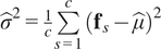
 as the number of channels of the multi-channel spatial feature) goes through the process of computation of mean
$ \hat{\mu}=\frac{1}{c}\sum \limits_{s=1}^c{\mathbf{f}}_s $
as the number of channels of the multi-channel spatial feature) goes through the process of computation of mean
$ \hat{\mu}=\frac{1}{c}\sum \limits_{s=1}^c{\mathbf{f}}_s $
 and variance
$ {\hat{\sigma}}^2=\frac{1}{c}\sum \limits_{s=1}^c{\left({\mathbf{f}}_s-\hat{\mu}\right)}^2 $
and variance
$ {\hat{\sigma}}^2=\frac{1}{c}\sum \limits_{s=1}^c{\left({\mathbf{f}}_s-\hat{\mu}\right)}^2 $
 . The channel mean
$ \hat{\mu} $
. The channel mean
$ \hat{\mu} $
 is then adjusted by a learnable offset
$ \delta $
is then adjusted by a learnable offset
$ \delta $
 to learn
$ \psi =\delta +\hat{\mu} $
to learn
$ \psi =\delta +\hat{\mu} $
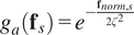
 . Then, the attention
$ {g}_a\left({\mathbf{f}}_s\right) $
. Then, the attention
$ {g}_a\left({\mathbf{f}}_s\right) $
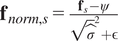
 is computed through normalized
$ {\mathbf{f}}_s $
is computed through normalized
$ {\mathbf{f}}_s $
 ,
$ {\mathbf{f}}_{\mathit{\operatorname{norm}},s} $
,
$ {\mathbf{f}}_{\mathit{\operatorname{norm}},s} $
 , where
$ {\mathbf{f}}_{\mathit{\operatorname{norm}},s}=\frac{{\mathbf{f}}_s-\psi }{{\sqrt{\hat{\sigma}}}^2+\unicode{x025B}} $
, where
$ {\mathbf{f}}_{\mathit{\operatorname{norm}},s}=\frac{{\mathbf{f}}_s-\psi }{{\sqrt{\hat{\sigma}}}^2+\unicode{x025B}} $
 :
$ {g}_a\left({\mathbf{f}}_s\right)={e}^{-\frac{{\mathbf{f}}_{\mathit{\operatorname{norm}},s}}{2{\zeta}^2}} $
:
$ {g}_a\left({\mathbf{f}}_s\right)={e}^{-\frac{{\mathbf{f}}_{\mathit{\operatorname{norm}},s}}{2{\zeta}^2}} $
 , with a small
$ \unicode{x025B} >0 $
, with a small
$ \unicode{x025B} >0 $
 .
.
The output of the Gaussian adaptive attention block
$ \mathbf{G} $
 is described as:

3.3. Three-dimensional positional encoder
Three-dimensional positional encoder
$ \mathbf{P} $
 employs Fourier based positional encoding on 3D coordinate points (Tancik et al., Reference Tancik, Srinivasan, Mildenhall, Fridovich-Keil, Raghavan, Singhal, Ramamoorthi, Barron and Ng2020). Considering
$ \mathbf{v}=\left(x,y,h\right) $
employs Fourier based positional encoding on 3D coordinate points (Tancik et al., Reference Tancik, Srinivasan, Mildenhall, Fridovich-Keil, Raghavan, Singhal, Ramamoorthi, Barron and Ng2020). Considering
$ \mathbf{v}=\left(x,y,h\right) $
 to denote a 3D coordinate point, with
$ {x}^{(c)}=\left(x,y\right) $
to denote a 3D coordinate point, with
$ {x}^{(c)}=\left(x,y\right) $
 being a point in the 2D coordinate space
$ {\mathbf{X}}_c $
being a point in the 2D coordinate space
$ {\mathbf{X}}_c $
 , and
$ h $
, and
$ h $
 the altitude of the corresponding modality, the output of the 3D positional encoder is:
$ \mathbf{P}\left(\mathbf{v}\right)=\left[\cdots, \cos \left(2{\pi \sigma}^{j/m}\mathbf{v}\right),\sin \left(2{\pi \sigma}^{j/m}\mathbf{v}\right),\cdots \right] $
the altitude of the corresponding modality, the output of the 3D positional encoder is:
$ \mathbf{P}\left(\mathbf{v}\right)=\left[\cdots, \cos \left(2{\pi \sigma}^{j/m}\mathbf{v}\right),\sin \left(2{\pi \sigma}^{j/m}\mathbf{v}\right),\cdots \right] $
 for
$ j\in \left\{0,1,\cdots, m-1\right\} $
for
$ j\in \left\{0,1,\cdots, m-1\right\} $
 , where
$ m $
, where
$ m $
 denotes the number of frequencies of the learned Fourier features, and
$ \sigma $
denotes the number of frequencies of the learned Fourier features, and
$ \sigma $
 denotes the frequency constant.
3.4. Kolmogorov-Arnold network
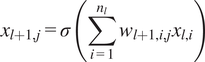
Traditional multi-layer perceptrons (MLPs) model non-linearity through fixed activation functions on nodes (Hornik et al., Reference Hornik, Stinchcombe and White1989), whereas KANs employ learnable activation functions on edges (Z Liu et al., Reference Liu, Wang, Vaidya, Ruehle, Halverson, Soljacic, Hou and Tegmark2025). There is no linear weight whatsoever in KANs, each weight parameter is substituted with a univariate function that is parameterized as a spline function instead (Boor, Reference Boor1978). For a traditional MLP, the output at node
$ j $
 of layer
$ l+1 $
of layer
$ l+1 $
 , can be defined as
with
$ \sigma $
 as a non-linear activation function. For a KAN, the output at node
$ j $
as a non-linear activation function. For a KAN, the output at node
$ j $
 of layer
$ l+1 $
of layer
$ l+1 $
 , can be defined as

where the non-linear function
$ \phi $
 can be defined as
$ \phi (x)=w\left(b(x)+\mathrm{spline}(x)\right) $
can be defined as
$ \phi (x)=w\left(b(x)+\mathrm{spline}(x)\right) $
 , with
$ b(x)=\mathrm{silu}(x)=x/\left(1+{e}^{-x}\right) $
, with
$ b(x)=\mathrm{silu}(x)=x/\left(1+{e}^{-x}\right) $
 and
$ \mathrm{spline}(x) $
and
$ \mathrm{spline}(x) $
 a linear combination of B-splines,
$ {\sum}_i{c}_i{B}_i(x) $
a linear combination of B-splines,
$ {\sum}_i{c}_i{B}_i(x) $
 with trainable
$ {c}_i $
with trainable
$ {c}_i $
 ‘s.
‘s.
3.5. Local implicit image function
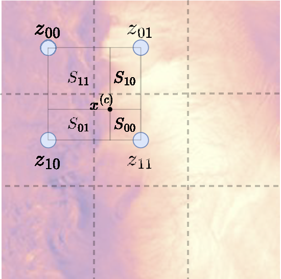
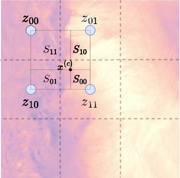
Local implicit image function (LIIF) (Chen et al., Reference Chen, Liu and Wang2021) is a deep learning-based continuous representation method from a discrete image or a multi-channel two-dimensional feature representation. A decoding function
$ {\mathbf{D}}_{\theta, liif} $
 is typically parameterized as an MLP and takes the form
$ s={\mathbf{D}}_{\theta, liif}\left(z,x\right) $
is typically parameterized as an MLP and takes the form
$ s={\mathbf{D}}_{\theta, liif}\left(z,x\right) $
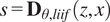 , where
$ z $
, where
$ z $
 is the observation of image pixel values or features at a 2D coordinate point
$ x $
is the observation of image pixel values or features at a 2D coordinate point
$ x $
 . Consider, our objective is to predict the output at point
$ {x}^{(c)} $
. Consider, our objective is to predict the output at point
$ {x}^{(c)} $
 , with observed features
$ {z}_t $
, with observed features
$ {z}_t $
 at neighboring coordinate points
$ {x}^{(t)},t=\left\{00,01,10,11\right\} $
at neighboring coordinate points
$ {x}^{(t)},t=\left\{00,01,10,11\right\} $
 .
$ {S}_t $
.
$ {S}_t $
 is the area of the rectangle between
$ {x}^{(c)} $
is the area of the rectangle between
$ {x}^{(c)} $
 and
$ {x}^{\left({t}^{\prime}\right)} $
and
$ {x}^{\left({t}^{\prime}\right)} $
 where
$ {t}^{\prime } $
where
$ {t}^{\prime } $
 is diagonal to
$ t $
is diagonal to
$ t $
 (i.e.
$ 00 $
(i.e.
$ 00 $
 to
$ 11 $
to
$ 11 $
 ,
$ 10 $
,
$ 10 $
 to
$ 01 $
to
$ 01 $
 ). Then, LIIF predicts the output at
$ {x}^{(c)} $
). Then, LIIF predicts the output at
$ {x}^{(c)} $
 as:
as:

$ S={\sum}_t{S}_t $
 is the total area of the four rectangles. Figure 1 illustrates this area-based interpolation through
$ {\mathbf{D}}_{\theta, liif} $
is the total area of the four rectangles. Figure 1 illustrates this area-based interpolation through
$ {\mathbf{D}}_{\theta, liif} $
 . Instead of applying the area-based interpolation through
$ {\mathbf{D}}_{\theta, liif} $
. Instead of applying the area-based interpolation through
$ {\mathbf{D}}_{\theta, liif} $
 directly on the input image pixels, multi-channel features
$ {z}_t $
directly on the input image pixels, multi-channel features
$ {z}_t $
 are first extracted using an EDSR (Lim et al., Reference Lim, Son, Kim, Nah and Lee2017) model and then decoded through
$ {\mathbf{D}}_{\theta, liif} $
are first extracted using an EDSR (Lim et al., Reference Lim, Son, Kim, Nah and Lee2017) model and then decoded through
$ {\mathbf{D}}_{\theta, liif} $
 .
.
LIIF method.
4. Problem statement
Let
$ {\mathbf{x}}_k^H\in {\mathcal{M}}_k^H\subset {\unicode{x211D}}^{h\times w} $
 denote the discrete high resolution data representation of modality
$ k $
denote the discrete high resolution data representation of modality
$ k $
 with
$ {\mathcal{M}}_k^H $
with
$ {\mathcal{M}}_k^H $
 being the discrete high resolution data space of modality
$ k $
being the discrete high resolution data space of modality
$ k $
 . We aim to achieve simultaneous data dimension reduction and cross-modal/altitude continuous reconstruction of this data instance. Our goal is to design a model capable of pertaining the following tasks:
-
1. Data Dimension Reduction: Execute $ {\mathbf{x}}_k^H\to {\mathbf{x}}_k^L\in {\mathcal{M}}_k^L\subset {\unicode{x211D}}^{\frac{h}{d}\times \frac{w}{d}} $
 , where
$ {\mathbf{x}}_k^L $
represents the discrete low resolution representation of
$ {\mathbf{x}}_k^H $
with
$ {\mathcal{M}}_k^L $
being the discrete low resolution data space of modality
$ k $
and
$ d $
being the dimension reduction factor.
, where
$ {\mathbf{x}}_k^L $
represents the discrete low resolution representation of
$ {\mathbf{x}}_k^H $
with
$ {\mathcal{M}}_k^L $
being the discrete low resolution data space of modality
$ k $
and
$ d $
being the dimension reduction factor. -
2. Cross-Altitude/Modality Continuous Reconstruction: Execute $ {\mathbf{x}}_k^L\to {\mathbf{x}}_{l\ne k}^C\left({x}^{(c)}\right)\in {\mathcal{M}}_l^C\left({x}^{(c)}\right)\subset \unicode{x211D} $
. Let,
$ {x}^{(c)}\in {\mathbf{X}}_c $
be any coordinate point in the continuous 2D coordinate space
$ {\mathbf{X}}_c $
. Here
$ {\mathbf{x}}_l^C\left({x}^{(c)}\right) $
represents the target value at coordinate point
$ {x}^{(c)} $
for modality
$ l $
and
$ {\mathcal{M}}_l^C\left({x}^{(c)}\right) $
represents the data space of target values. The continuous nature of
$ {\mathbf{X}}_c $
makes this task a continuous reconstruction from low dimensional representation
$ {\mathbf{x}}_k^L $
.






We will use cross/multi-altitude and cross/multi-modality interchangably throughout the rest of the paper.
5. Method
Overview. Our proposed encoder-decoder (transfer)-decoder (continuous reconstructor) framework,
$ {\mathbf{T}}_{\theta } $
 , comprises three primary components:
-
• encoder: The three-dimensional implicit neural network, $ {\mathbf{E}}_{\phi } $
, reduces dimension of the data from input modality/altitude
$ {\mathbf{x}}_{in}^H $
to
$ {\mathbf{x}}_{in}^L $
. This compression is optimized to retain sufficient information for downstream tasks.
$ {h}_{in} $
being the altitude of the input modality, we can define the encoder mapping:
$ {\mathbf{x}}_{in}^L={\mathbf{E}}_{\phi}\left({\mathbf{x}}_{in}^H,{h}_{in}\right),{\mathbf{E}}_{\phi }:{\mathcal{M}}_{in}^H\to {\mathcal{M}}_{in}^L $
. -
• decoder (transfer): The three-dimensional implicit neural network, $ {\mathbf{D}}_{tr} $
, transforms the discrete low resolution representation of the input modality/altitude
$ {\mathbf{x}}_{in}^L $
to the discrete high resolution representation of the target modality/altitude
$ {\mathbf{x}}_{out}^H $
.
$ {h}_{out} $
being the altitude of the target modality, we can define the mapping:
$ {\mathbf{x}}_{out}^H={\mathbf{D}}_{tr}\left({\mathbf{x}}_{in}^L,{h}_{out}\right),{\mathbf{D}}_{tr}:{\mathcal{M}}_{in}^L\to {\mathcal{M}}_{out}^H $
. -
• decoder (continuous reconstructor): The implicit continuous decoder, $ {\mathbf{D}}_{cr} $
, that utilizes the modality/altitude-transferred discrete high resolution representation
$ {\mathbf{x}}_{out}^H $
to predict wind data at specific coordinate
$ {\mathbf{x}}_{out}^C\left({x}^{(c)}\right) $
.We can define this mapping:
$ {\mathbf{x}}_{out}^C\left({x}^{(c)}\right)={\mathbf{D}}_{cr}\left({\mathbf{x}}_{out}^H,{x}^{(c)}\right),{\mathbf{D}}_{cr}:{\mathcal{M}}_{out}^H\times {\mathbf{X}}_c\to {\mathcal{M}}_{out}^C $
.









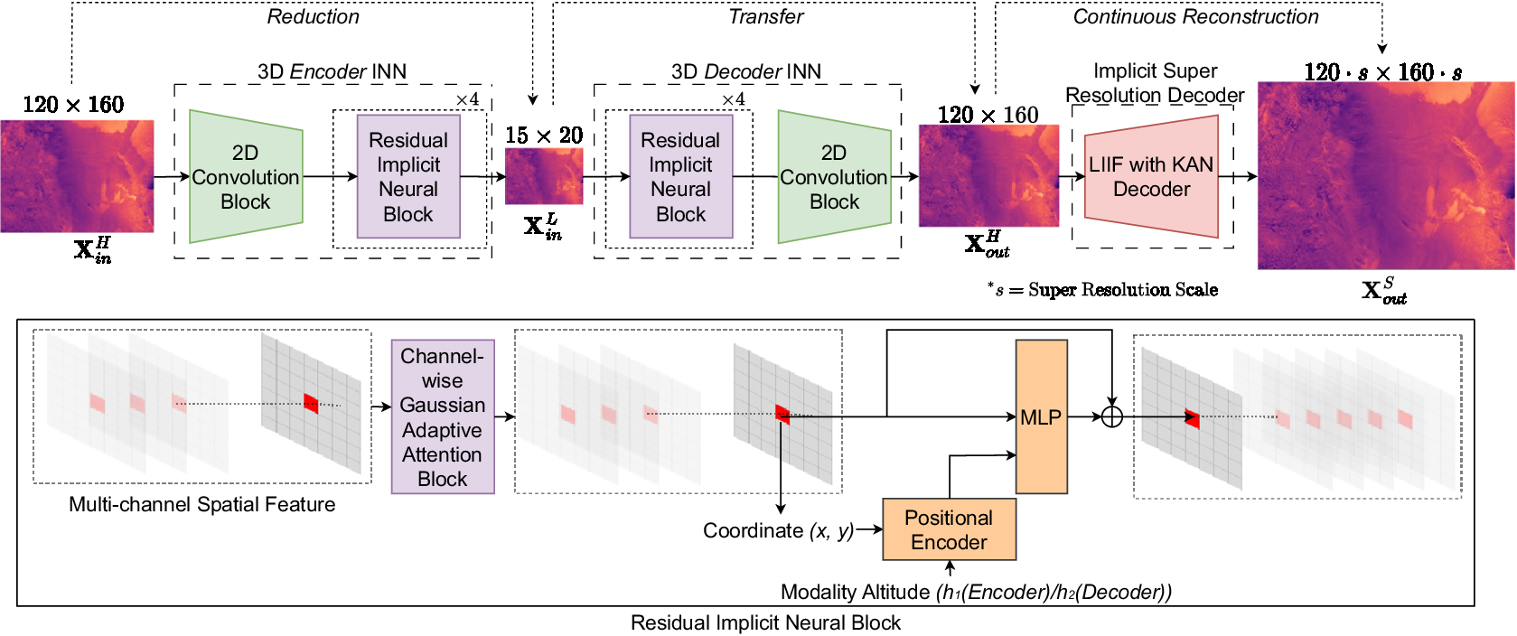
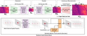
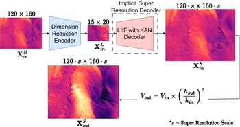
Figure 2 summarizes the proposed model,
$ {\mathbf{T}}_{\theta}:= {\mathbf{D}}_{cr}\circ {\mathbf{D}}_{tr}\circ {\mathbf{E}}_{\phi } $
 . We describe the encoder-decoder (transfer) segment,
$ {\mathbf{D}}_{tr}\circ {\mathbf{E}}_{\phi } $
. We describe the encoder-decoder (transfer) segment,
$ {\mathbf{D}}_{tr}\circ {\mathbf{E}}_{\phi } $
 in Section 5.1 and decoder (continuous reconstructor) segment
$ {\mathbf{D}}_{cr} $
in Section 5.1 and decoder (continuous reconstructor) segment
$ {\mathbf{D}}_{cr} $
 in Section 5.2.
Overview of the proposed method, which jointly enables data reduction, transfer across modalities, and continuous representation and arbitrary-scale super resolution.
5.1. Three-dimensional encoder-transfer implicit neural network
3D ETINN (Three-Dimensional Encoder-Transfer Implicit Neural Network) consists of the first two segments of the overall framework: (i) encoder: a 3D encoder INN,
$ {\mathbf{E}}_{\phi } $
 , and (ii) decoder (transfer): a 3D decoder (transfer) INN,
$ {\mathbf{D}}_{tr} $
, and (ii) decoder (transfer): a 3D decoder (transfer) INN,
$ {\mathbf{D}}_{tr} $
 . Both the encoder and decoder (transfer) consist of (i) a convolution block,
$ \mathbf{Conv} $
. Both the encoder and decoder (transfer) consist of (i) a convolution block,
$ \mathbf{Conv} $
 , and several (ii) residual implicit neural blocks,
$ {\mathbf{R}}_{inn} $
, and several (ii) residual implicit neural blocks,
$ {\mathbf{R}}_{inn} $
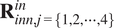
 . 3D encoder INN,
$ {\mathbf{E}}_{\phi } $
. 3D encoder INN,
$ {\mathbf{E}}_{\phi } $
 , consists of a convolutional block,
$ {\mathbf{Conv}}_{in} $
, consists of a convolutional block,
$ {\mathbf{Conv}}_{in} $
 , followed by several residual implicit neural blocks,
$ {\mathbf{R}}_{in n,j=\left\{1,2,\cdots, 4\right\}}^{in} $
, followed by several residual implicit neural blocks,
$ {\mathbf{R}}_{in n,j=\left\{1,2,\cdots, 4\right\}}^{in} $
 , and can be described as

3D decoder (transfer) INN,
$ {\mathbf{D}}_{tr} $
 , consists of several residual implicit neural blocks,
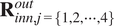
$ {\mathbf{R}}_{inn,j=\left\{1,2,\cdots, 4\right\}}^{out} $
, consists of several residual implicit neural blocks,
$ {\mathbf{R}}_{inn,j=\left\{1,2,\cdots, 4\right\}}^{out} $
 , followed by a convolutional block,
$ {\mathbf{Conv}}_{out} $
, followed by a convolutional block,
$ {\mathbf{Conv}}_{out} $
 , and can be described as

We employed four residual implicit neural blocks in our proposed method. We varied the number of residual implicit neural blocks in our method and report the results in Supplementary Materials.
5.1.1. Residual implicit neural block
Residual implicit neural block
$ {\mathbf{R}}_{inn} $
 consists of a Gaussian adaptive attention block
$ \mathbf{G} $
consists of a Gaussian adaptive attention block
$ \mathbf{G} $
 , a three-dimensional positional encoder
$ \mathbf{P} $
, a three-dimensional positional encoder
$ \mathbf{P} $
 , and a 2-layer MLP network
$ {\mathbf{D}}_{inn} $
, and a 2-layer MLP network
$ {\mathbf{D}}_{inn} $
 . Conventional implicit neural networks use a two-dimensional positional encoder to process grid-like 2D data, such as images. In contrast, the residual implicit neural block operates on two-dimensional data while utilizing a positional encoder,
$ \mathbf{P} $
. Conventional implicit neural networks use a two-dimensional positional encoder to process grid-like 2D data, such as images. In contrast, the residual implicit neural block operates on two-dimensional data while utilizing a positional encoder,
$ \mathbf{P} $
 , that accepts three-dimensional coordinate points as input. This approach allows the flexibility in transforming 2D data across modalities.
Let the input to
$ {\mathbf{R}}_{inn} $
 be the multi-channel two-dimensional spatial feature,
$ F\in {\unicode{x211D}}^{c\times \frac{h}{d}\times \frac{w}{d}} $
be the multi-channel two-dimensional spatial feature,
$ F\in {\unicode{x211D}}^{c\times \frac{h}{d}\times \frac{w}{d}} $
 , and
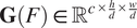
$ \mathbf{G}(F)\in {\unicode{x211D}}^{c\times \frac{h}{d}\times \frac{w}{d}} $
, and
$ \mathbf{G}(F)\in {\unicode{x211D}}^{c\times \frac{h}{d}\times \frac{w}{d}} $
 be the output of the Gaussian adaptive attention block,
$ \mathbf{G} $
be the output of the Gaussian adaptive attention block,
$ \mathbf{G} $
 .
$ \mathbf{G}(F) $
.
$ \mathbf{G}(F) $
 can be considered as a stack of
$ \frac{hw}{d^2} $
can be considered as a stack of
$ \frac{hw}{d^2} $
 numbers of
$ c $
numbers of
$ c $
 -dimensional features,
$ {\left[{gf}_{x^{(c)}}\right]}_{\frac{hw}{d^2}} $
-dimensional features,
$ {\left[{gf}_{x^{(c)}}\right]}_{\frac{hw}{d^2}} $
 (visually illustrated in the lower block of Figure 2). Let
$ {gf}_{x^{(c)}}\in {\unicode{x211D}}^c $
(visually illustrated in the lower block of Figure 2). Let
$ {gf}_{x^{(c)}}\in {\unicode{x211D}}^c $
 be the local feature at 2D coordinate point
$ {x}^{(c)} $
be the local feature at 2D coordinate point
$ {x}^{(c)} $
 of
$ \mathbf{G}(F) $
of
$ \mathbf{G}(F) $
 , where
$ c $
, where
$ c $
 is the number of channels for the spatial feature.
$ {gf}_{x^{(c)}} $
is the number of channels for the spatial feature.
$ {gf}_{x^{(c)}} $
 is then transformed into
$ {\mathbf{D}}_{inn}\left(\left\{{gf}_{x^{(c)}},\mathbf{P}\left(x,y,h\right)\right\}\right)+{gf}_{x^{(c)}} $
is then transformed into
$ {\mathbf{D}}_{inn}\left(\left\{{gf}_{x^{(c)}},\mathbf{P}\left(x,y,h\right)\right\}\right)+{gf}_{x^{(c)}} $
 , where
$ {\mathbf{D}}_{inn} $
, where
$ {\mathbf{D}}_{inn} $
 is a 2-layer MLP network,
$ h $
is a 2-layer MLP network,
$ h $
 is the altitude for the corresponding modality. Similar transformation is done for all those
$ \frac{hw}{d^2} $
is the altitude for the corresponding modality. Similar transformation is done for all those
$ \frac{hw}{d^2} $
 numbers of
$ gf $
numbers of
$ gf $
 ‘s. So, the feature transformation through
$ {\mathbf{R}}_{inn} $
‘s. So, the feature transformation through
$ {\mathbf{R}}_{inn} $
 can be described as a two-step transformation:
-
1. Feature transformation through Gaussian Adaptive Attention, $ F\to \mathbf{G}(F) $
. -
2. Transformation of $ \mathbf{G}(F) $
through residual neural network:



5.2. Implicit super-resolution decoder
Implicit super-resolution decoder,
$ {\mathbf{D}}_{cr}:{\mathcal{M}}_k^H\times {\mathbf{X}}_c\to {\mathcal{M}}_k^C $
 , takes the transformed discrete high-resolution representation
$ {\mathbf{X}}_k^H $
, takes the transformed discrete high-resolution representation
$ {\mathbf{X}}_k^H $
 and any 2D coordinate point
$ {x}^{(c)}\in {\mathbf{X}}_c $
and any 2D coordinate point
$ {x}^{(c)}\in {\mathbf{X}}_c $
 and predicts the output at coordinate point
$ {x}^{(c)} $
and predicts the output at coordinate point
$ {x}^{(c)} $
 ,
$ {\mathbf{x}}_k^C\left({x}^{(c)}\right) $
,
$ {\mathbf{x}}_k^C\left({x}^{(c)}\right) $
 . We use a modified version of local implicit image function (LIIF) based decoder, which is a coordinate based decoding approach (Chen et al., Reference Chen, Liu and Wang2021). The original LIIF decoder primarily consists of two components: (i) EDSR-based feature encoder (Lim et al., Reference Lim, Son, Kim, Nah and Lee2017), and a (ii) MLP network. In our modified LIIF-KAN decoder, we replace the MLP network with a KAN (Kolmogorov-Arnold Network)-based decoder (Liu et al., Reference Liu, Wang, Vaidya, Ruehle, Halverson, Soljacic, Hou and Tegmark2025).
Decoder (continuous reconstructor)
: EDSR-based (Lim et al., Reference Lim, Son, Kim, Nah and Lee2017) feature encoder,
$ \mathbf{FE} $
 , encodes
$ {\mathcal{M}}_{out}^H $
, encodes
$ {\mathcal{M}}_{out}^H $
 into the encoded feature space
$ {\mathcal{M}}_{out}^F $
into the encoded feature space
$ {\mathcal{M}}_{out}^F $
 ,
$ \mathbf{FE}:{\mathcal{M}}_{out}^H\to {\mathcal{M}}_{out}^F $
,
$ \mathbf{FE}:{\mathcal{M}}_{out}^H\to {\mathcal{M}}_{out}^F $
 . The KAN-based decoder,
$ {\mathbf{D}}_{kan} $
. The KAN-based decoder,
$ {\mathbf{D}}_{kan} $
 , then predicts the output at coordinate point
$ {x}^{(c)} $
, then predicts the output at coordinate point
$ {x}^{(c)} $
 following the similar methodology followed in LIIF (Chen et al., Reference Chen, Liu and Wang2021). The overall continuous reconstruction can be described as:
$ {\mathbf{x}}_{out}^C\left({x}^{(c)}\right)=\left({\mathbf{D}}_{kan}\circ \mathbf{FE}\right)\left({\mathbf{x}}_{out}^H,{x}^{(c)}\right) $
following the similar methodology followed in LIIF (Chen et al., Reference Chen, Liu and Wang2021). The overall continuous reconstruction can be described as:
$ {\mathbf{x}}_{out}^C\left({x}^{(c)}\right)=\left({\mathbf{D}}_{kan}\circ \mathbf{FE}\right)\left({\mathbf{x}}_{out}^H,{x}^{(c)}\right) $
 .
.
5.3. Cross-altitude prediction
Let,
$ {\mathbf{x}}_{in}^H $
 be a discrete high-dimensional datapoint at altitude
$ {h}_{in} $
be a discrete high-dimensional datapoint at altitude
$ {h}_{in} $
 . For simultaneous dimension reduction and continuous cross-altitude reconstruction through super-resolution, we need to infer discrete low-resolution representation
$ {\mathbf{x}}_{in}^L $
. For simultaneous dimension reduction and continuous cross-altitude reconstruction through super-resolution, we need to infer discrete low-resolution representation
$ {\mathbf{x}}_{in}^L $
 , and
$ {\mathbf{x}}_{out}^C\left({x}^{(c)}\right) $
, and
$ {\mathbf{x}}_{out}^C\left({x}^{(c)}\right) $
 , where
$ {x}^{(c)} $
, where
$ {x}^{(c)} $
 can be any 2D coordinate point in
$ {\mathbf{X}}_c $
can be any 2D coordinate point in
$ {\mathbf{X}}_c $
 at altitude
$ {h}_{out} $
at altitude
$ {h}_{out} $
 . Then,


$ {h}_{in}\ne {h}_{out} $
 refers to the cross-altitude prediction scenario. At a super-resolution scale
$ s $
refers to the cross-altitude prediction scenario. At a super-resolution scale
$ s $
 , we evaluate
$ {\mathbf{D}}_{KAN} $
, we evaluate
$ {\mathbf{D}}_{KAN} $
 on
$ {s}^2 hw $
on
$ {s}^2 hw $
 number of different
$ {x}^{(c)}\in {\mathbf{X}}_c $
number of different
$ {x}^{(c)}\in {\mathbf{X}}_c $
 , resulting in a super-resolved output with dimension
$ {\unicode{x211D}}^{sh\times sw} $
, resulting in a super-resolved output with dimension
$ {\unicode{x211D}}^{sh\times sw} $
 .
.
6. Experiments
We first introduce the wind dataset that we used to evaluate our proposed model. Then we continue to elaborate the optimization procedure and obtained results.
6.1. Wind data
National Renewable Energy Laboratory’s Wind Integration National Database (WIND) Toolkit provides high spatial and temporal resolution wind power, wind power forecasting, and meteorological data for over 126,000 locations across the continental United States during a 7-year span (Draxl et al., Reference Draxl, Clifton, Hodge and McCaa2015). The simulated forecasts were developed using the Weather Research and Forecasting Model, which operates on a 2-kilometer (km) by 2-kilometer (km) grid with a 10-meter(m) resolution from the ground to
$ 200\;\mathrm{m} $
 above ground with several temporal resolutions available at 1-hour, 4-hour, 6-hour, and day-ahead forecast horizons. The spatial resolution of the WIND Toolkit is
$ 2\;\mathrm{km}\times 1\;\mathrm{hr} $
above ground with several temporal resolutions available at 1-hour, 4-hour, 6-hour, and day-ahead forecast horizons. The spatial resolution of the WIND Toolkit is
$ 2\;\mathrm{km}\times 1\;\mathrm{hr} $
 in spatio-temporal resolution. As a result, the wind dataset size is
$ 1602\left(\mathrm{latitude}\right)\times 2976\left(\mathrm{longitude}\right)\times 61368\left(\mathrm{number}\ \mathrm{of}\ \mathrm{instances}\right) $
in spatio-temporal resolution. As a result, the wind dataset size is
$ 1602\left(\mathrm{latitude}\right)\times 2976\left(\mathrm{longitude}\right)\times 61368\left(\mathrm{number}\ \mathrm{of}\ \mathrm{instances}\right) $
 , or almost 1.2 TB per wind component (wind data at different heights). We randomly cropped data to reduce the resolution to
$ 1500\left(\mathrm{latitude}\right)\times 2000\left(\mathrm{longitude}\right) $
, or almost 1.2 TB per wind component (wind data at different heights). We randomly cropped data to reduce the resolution to
$ 1500\left(\mathrm{latitude}\right)\times 2000\left(\mathrm{longitude}\right) $
 for each time instance. Wind velocity components at specific direction were determined using the wind speed and direction at a specific height. For example, if wind speed at height
$ h $
for each time instance. Wind velocity components at specific direction were determined using the wind speed and direction at a specific height. For example, if wind speed at height
$ h $
 is
$ V $
is
$ V $
 at an angle
$ \theta {}^{\circ} $
at an angle
$ \theta {}^{\circ} $
 with northern direction, the northern and eastern components are
$ u=V\cos \theta {}^{\circ},v=V\sin \theta {}^{\circ} $
with northern direction, the northern and eastern components are
$ u=V\cos \theta {}^{\circ},v=V\sin \theta {}^{\circ} $
 accordingly. In this paper, we only report the results with the northern projection of wind speed data.
6.2. Experimental setup
6.2.1. Dataset
To evaluate the continuous reconstruction capability of our proposed method, we created a dataset for multi-modal super-resolution tasks using simulated wind data discussed in Section 6.1.
Dataset creation
From the total
$ 61368 $
 data instances at different timepoints, we randomly sampled
$ 4000 $
data instances at different timepoints, we randomly sampled
$ 4000 $
 data points from various timestamps at heights of
$ 10\;\mathrm{m},60\;\mathrm{m},160\;\mathrm{m} $
data points from various timestamps at heights of
$ 10\;\mathrm{m},60\;\mathrm{m},160\;\mathrm{m} $
 and
$ 200\;\mathrm{m} $
and
$ 200\;\mathrm{m} $
 . We used
$ 3000 $
. We used
$ 3000 $
 data points for training,
$ 200 $
data points for training,
$ 200 $
 for validation and
$ 800 $
for validation and
$ 800 $
 for testing.
Data sample processing
We used bicubic interpolation to generate a pair of discrete and continuous high-resolution samples for each instance. For example, if the discrete input dimension is
$ 120\times 160 $
 and the super-resolution scale is
$ 2.5\times $
and the super-resolution scale is
$ 2.5\times $
 , the continuous output dimension is
$ 300\times 400 $
, the continuous output dimension is
$ 300\times 400 $
 . Data sample creation for training and validation/test has been conducted differently for better learning of the model.
-
• Train: During training, the continuous high-resolution sample is created by randomly cropping from the actual $ 1500\times 2000 $
resolution data sample and then generating the discrete high-resolution sample via bicubic interpolation. The discrete high-resolution dimension was set to
$ 120\times 160 $
, with super-resolution scales ranging from
$ 1\times $
to
$ 4\times $
. -
• Validation/Test: At testing, we split the original $ 1500\times 2000 $
resolution data into
$ 4 $
data samples of resolution
$ 750\times 1000 $
by splitting them evenly into four regions. As a result, the test dataset consists of
$ 3200 $
data samples, each with a dimension of
$ 750\times 1000 $
. To avoid randomness during testing, both continuous and discrete high-resolution samples were generated by bicubic interpolation from this data sample with dimension
$ 750\times 1000 $
. For example, if the task is to super-resolve the discrete super-resolution sample of dimension
$ 120\times 160 $
to a super-resolution scale
$ 2.5\times $
(the continuous high-resolution sample dimension is
$ 300\times 400 $
), both the discrete and continuous high-resolution samples are generated through bicubic interpolation from the original cropped sample of dimension
$ 750\times 1000 $
.


6.2.2. Training details
Adam was adopted as the optimizer (Kingma and Ba, Reference Kingma, Ba, Bengio and LeCun2015), to train the model for
$ 600 $
 epochs. The learning rate during the optimization was set following the cyclical learning rate technique with a minimum learning rate of
$ {10}^{-5} $
epochs. The learning rate during the optimization was set following the cyclical learning rate technique with a minimum learning rate of
$ {10}^{-5} $
 and a maximum learning rate of
$ {10}^{-4} $
and a maximum learning rate of
$ {10}^{-4} $
 (Smith, Reference Smith2017). At super-resolution scale
$ s $
(Smith, Reference Smith2017). At super-resolution scale
$ s $
 , the super-resolution ground truth
$ {\mathbf{x}}_{out}^S $
, the super-resolution ground truth
$ {\mathbf{x}}_{out}^S $
 has a dimension of
$ sh\times sw $
has a dimension of
$ sh\times sw $
 . Coordinate-based implicit neural networks, e.g., LIIF (Y Chen et al., Reference Chen, Liu and Wang2021), predict outputs pixel-by-pixel instead of predicting the whole super-resolved image at a single forward pass. We randomly selected
$ 2048 $
. Coordinate-based implicit neural networks, e.g., LIIF (Y Chen et al., Reference Chen, Liu and Wang2021), predict outputs pixel-by-pixel instead of predicting the whole super-resolved image at a single forward pass. We randomly selected
$ 2048 $
 coordinate points, at each optimization step, among the
$ {s}^2 hw $
coordinate points, at each optimization step, among the
$ {s}^2 hw $
 coordinate points of the target super-resolved continuous representation, and optimized the parameters based on the predictions
$ {\hat{\mathbf{x}}}_{out}^C\left({x}^{(c)}\right) $
coordinate points of the target super-resolved continuous representation, and optimized the parameters based on the predictions
$ {\hat{\mathbf{x}}}_{out}^C\left({x}^{(c)}\right) $
 and the ground truth
$ {\mathbf{x}}_{out}^C\left({x}^{(c)}\right) $
and the ground truth
$ {\mathbf{x}}_{out}^C\left({x}^{(c)}\right) $
 on those coordinate points to extradite the optimization process. We used the
$ {L}_1 $
on those coordinate points to extradite the optimization process. We used the
$ {L}_1 $
 loss function,
$ {l}_1\left({\hat{\mathbf{x}}}_{out}^C,{\mathbf{x}}_{out}^C,{x}^{(c)}\right)=\mid {\mathbf{x}}_{out}^C\left({x}^{(c)}\right)-{\hat{\mathbf{x}}}_{out}^C\left({x}^{(c)}\right)\mid $
loss function,
$ {l}_1\left({\hat{\mathbf{x}}}_{out}^C,{\mathbf{x}}_{out}^C,{x}^{(c)}\right)=\mid {\mathbf{x}}_{out}^C\left({x}^{(c)}\right)-{\hat{\mathbf{x}}}_{out}^C\left({x}^{(c)}\right)\mid $
 , to optimize the model. It took about 12 hours to train the model on a workstation with a single NVIDIA A100 GPU.
6.2.3. Evaluation metrics
We employed two metrics to evaluate the continuous reconstruction through super resolution. Peak signal-to-noise ratio (PSNR) is the ratio of a signal’s maximum possible value (power) to the power of distorting noise that affects the quality of its representation. Structural similarity index (SSIM) is a perceptual metric that evaluates the degradation of image quality, which compares the spatial structures between the target image and reproduced image. For evaluation of the compression performance, we employed the Compression Ratio (CR) metric, which measures the ratio between the required memory for storing the compressed versus the uncompressed data. These evaluation metrics have been discussed in detail in the Supplementary Materials.
6.3. Results
6.3.1. Task
We evaluated the model’s continuous reconstruction capability by performing super-resolution at different scales on a test dataset containing 800 data points. As we split each data point into 4 regions, the total number of effective test data samples is 3200.
6.3.2. Setup
High-resolution input dimension was set to
$ 120\times 160 $
 , with a dimension reduction factor
$ d=8 $
, with a dimension reduction factor
$ d=8 $
 , yielding a low-resolution representation of
$ 15\times 20 $
, yielding a low-resolution representation of
$ 15\times 20 $
 . We focus on cross-altitude predictions where the input modality height
$ {h}_{in} $
. We focus on cross-altitude predictions where the input modality height
$ {h}_{in} $
 is closer to the ground (10 m, 60 m) and the output modality height
$ {h}_{out} $
is closer to the ground (10 m, 60 m) and the output modality height
$ {h}_{out} $
 is significantly higher (160 m, 200 m). Evaluation results for the opposite cross-altitude prediction scenarios have been discussed in the Supplementary Materials. Due to the lack of existing methodologies for simultaneous dimension reduction and reconstruction through super-resolution, we use the following three methods as baselines:
-
• MAINN (Multi-Altitude Implicit Neural Network): Multi-altitude simultaneous reduction and continuous reconstruction through a multi-modal implicit neural network (Qayyum et al., Reference Qayyum, Luo, Urban, Qian and Yoon2024). We trained 4 different models with combinations of data from (10 m, 160 m), (60 m, 160 m), (10 m, 200 m), and (60 m, 200 m) heights.
-
• GINO: Bicubic downscaling followed by Geometry-Informed Neural Operator (GINO) (Li et al., Reference Li, Kovachki, Choy, Li, Kossaifi, Otta, Nabian, Stadler, Hundt, Azizzadenesheli and Anandkumar2024).
-
• WindLaw: We used the wind power law $ {v}_1/{v}_2={\left({h}_1/{h}_2\right)}^{\alpha } $
with our proposed One Stone Three Bird (OSTB) model. We eliminated the 3D Decoder INN and trained four different models for four altitudes, and then used the wind power law for cross-altitude prediction.

6.3.3. Result summary
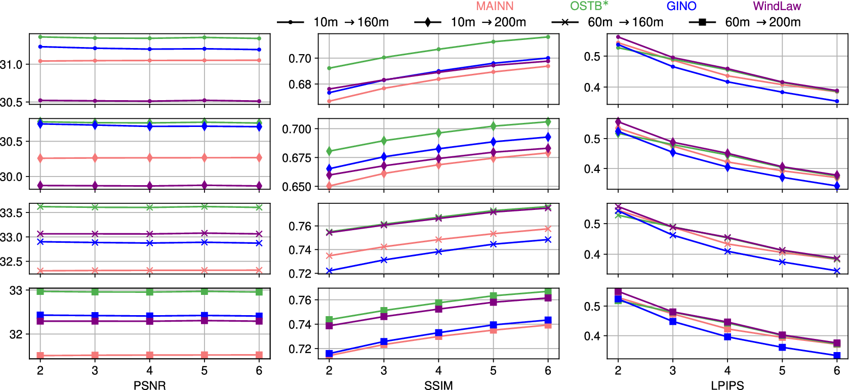
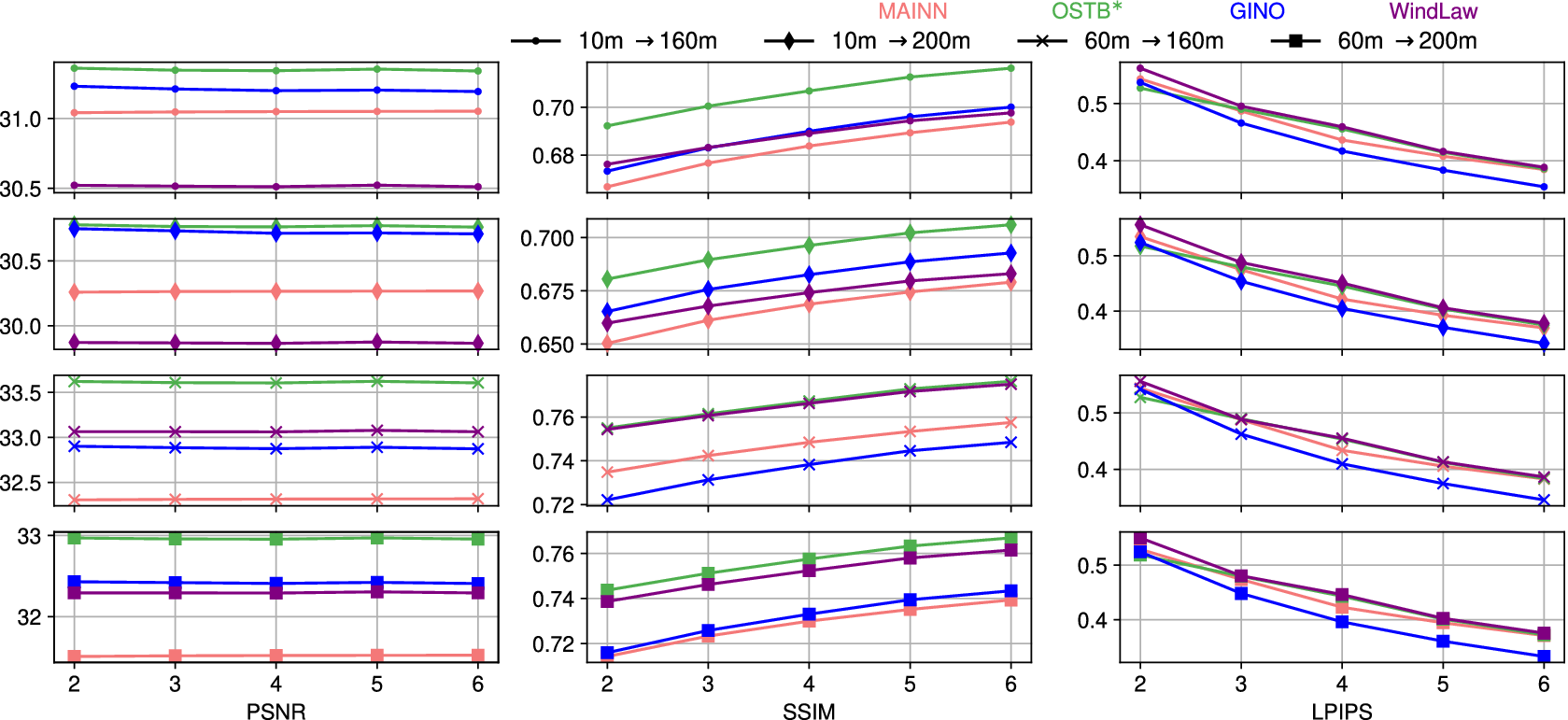
As shown in Figure 3, our model consistently outperforms all the baselines across all cross-altitude scenarios and super-resolution scales for PSNR and SSIM. Our model obtained low LPIPS for the super resolution scale
$ 2\times $
 , but obtained higher LPIPS for higher super-resolution scales. The GINO model obtained superior results in terms of LPIPS. Results for super-resolution scales
$ s\in \left[2,4\right] $
, but obtained higher LPIPS for higher super-resolution scales. The GINO model obtained superior results in terms of LPIPS. Results for super-resolution scales
$ s\in \left[2,4\right] $
 and
$ s\in \left[5,6\right] $
and
$ s\in \left[5,6\right] $
 respectively illustrate the results for in-distribution scales and out-of-distribution scales.
Comparative Results with Baselines.
$ x- $
 axis shows different super resolution scales for all three subplots, and
$ y- $
axis shows different super resolution scales for all three subplots, and
$ y- $
 axis shows the metric values (PSNR, SSIM and LPIPS metric values are shown in the three columns from left to right column accordingly). The 4 rows show the evaluation results in 4 different cross-altitude prediction scenarios:
$ 10\hskip0.42em m\to 160\hskip0.42em m $
axis shows the metric values (PSNR, SSIM and LPIPS metric values are shown in the three columns from left to right column accordingly). The 4 rows show the evaluation results in 4 different cross-altitude prediction scenarios:
$ 10\hskip0.42em m\to 160\hskip0.42em m $
 ,
$ 10\hskip0.42em m\to 200\hskip0.42em m $
,
$ 10\hskip0.42em m\to 200\hskip0.42em m $
 ,
$ 60\hskip0.52em m\to 160\hskip0.42em m, $
,
$ 60\hskip0.52em m\to 160\hskip0.42em m, $
 and
$ 60\hskip0.42em m\to 200\hskip0.42em m $
and
$ 60\hskip0.42em m\to 200\hskip0.42em m $
 from top to bottom row accordingly. For the WindLaw baseline, the displayed results are observed with
$ \alpha =0.16 $
from top to bottom row accordingly. For the WindLaw baseline, the displayed results are observed with
$ \alpha =0.16 $
 .
.
6.4. Additional Experiment 1: data compression
6.4.1. Task
We evaluate the data compression performance of our model and compare it against existing compression methods, focusing on cross-altitude prediction and reconstruction accuracy.
6.4.2. Setup
We employed the Prediction by Partial Matching (PPM) data compression algorithm with
$ \mu $
 -law encoding at various quantization levels (
$ Q $
-law encoding at various quantization levels (
$ Q $
 ) for data compression and reconstruction, as described in Moffat (Reference Moffat1990). Additionally, we tested bicubic interpolation for compressing and decompressing the data. For cross-altitude predictions, we used the wind power law
$ {v}_1/{v}_2={\left({h}_1/{h}_2\right)}^{\alpha } $
) for data compression and reconstruction, as described in Moffat (Reference Moffat1990). Additionally, we tested bicubic interpolation for compressing and decompressing the data. For cross-altitude predictions, we used the wind power law
$ {v}_1/{v}_2={\left({h}_1/{h}_2\right)}^{\alpha } $
 to transform the reconstructed data from one height to another for both PPM and bicubic methods. To assess performance, we measured the average compression ratio, PSNR, and SSIM over the test set. Since traditional compression methods lack super-resolution capabilities, we limit super-resolution comparison to the scale
$ s=1 $
to transform the reconstructed data from one height to another for both PPM and bicubic methods. To assess performance, we measured the average compression ratio, PSNR, and SSIM over the test set. Since traditional compression methods lack super-resolution capabilities, we limit super-resolution comparison to the scale
$ s=1 $
 for our model.
6.4.3. Result summary
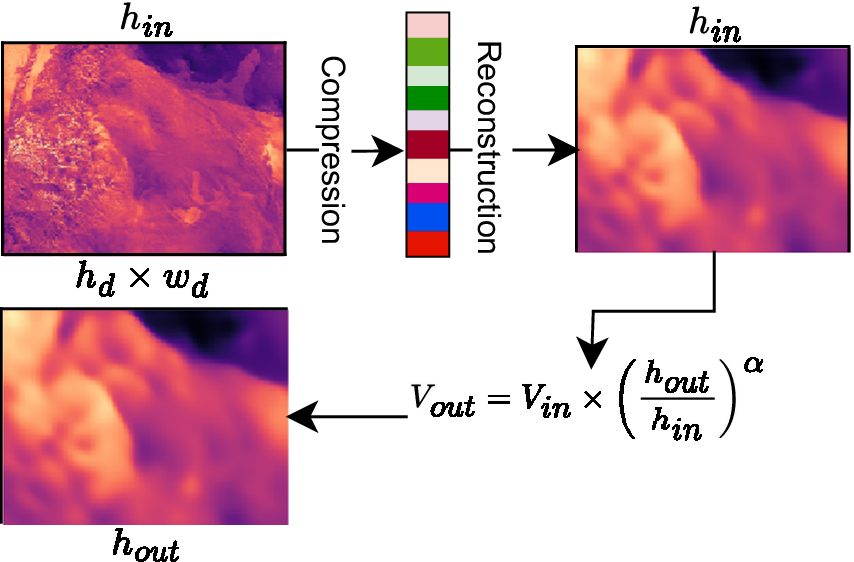
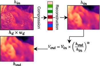
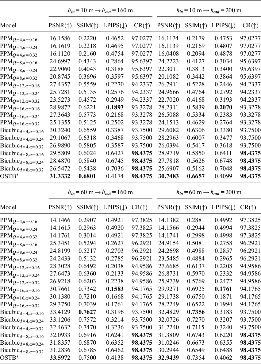
Figure 4 illustrates the cross-altitude prediction methodology of these methods, while Table 1 presents a detailed comparison. For cross-altitude predictions where the input modality height is 10 m, our model outperforms the baseline methods across three metrics—compression ratio, PSNR, and SSIM. In cases where the input modality height is 60 m, while our model does not achieve the best PSNR and SSIM, it significantly surpasses others in terms of compression ratio. For bicubic models with a reduction factor
$ d=4 $
 , the low-resolution dimension is
$ 30\times 40 $
, the low-resolution dimension is
$ 30\times 40 $
 . With a higher reduction factor (
$ d=8 $
. With a higher reduction factor (
$ d=8 $
 ), bicubic models achieve a compression ratio similar to ours but at the cost of lower PSNR and SSIM. Likewise, PPM models attain higher compression ratios at lower
$ Q $
), bicubic models achieve a compression ratio similar to ours but at the cost of lower PSNR and SSIM. Likewise, PPM models attain higher compression ratios at lower
$ Q $
 values, but at the expense of PSNR and SSIM. Only our model consistently delivers a high compression ratio alongside either the best or near-best PSNR and SSIM. Regarding the LPIPS metric, our model is outperformed by other models across all cross-altitude prediction scenarios, however their compression ratio is significantly higher than our model.
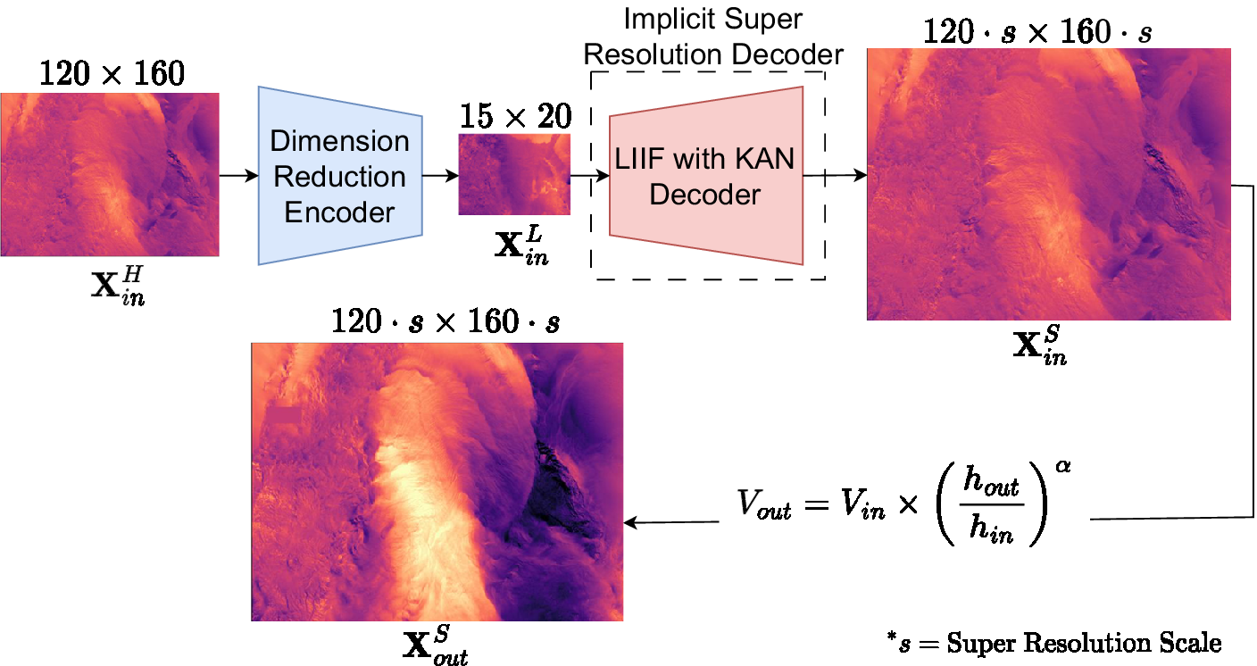
Data compression followed by cross-altitude prediction using wind power law.
Comparative compression performance at different cross-altitude prediction scenarios. Best performing methods are boldfaced according to respective metrics.
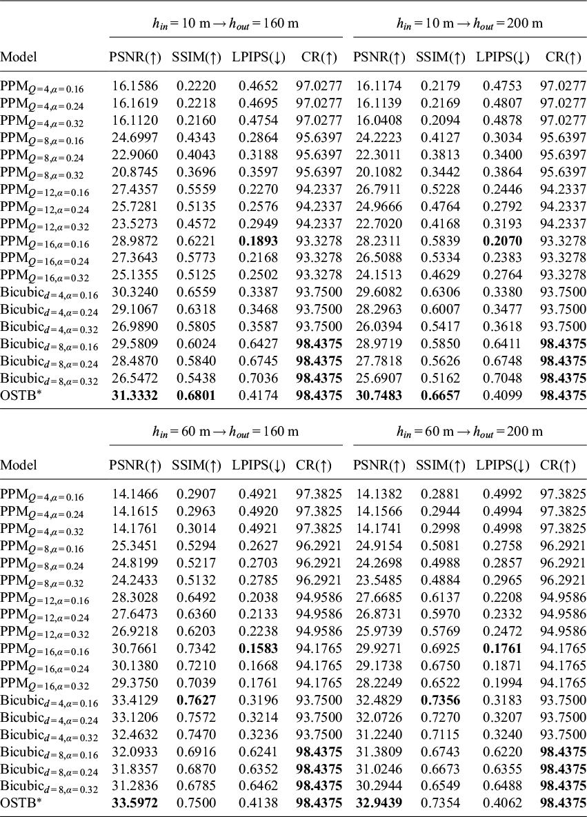
Table 1. Long description
Comparative compression performance at different cross-altitude prediction scenarios. Four different cross-altitude prediction scenarios have been evaluated and all cross-altitude prediction scenarios are from lower altitude to higher altitude.
6.5. Additional experiment 2: modality transfer
6.5.1. Task
We evaluate the performance of our model without the 3D ETINN segment by designing and training separate models for different altitude levels, then comparing them in cross-altitude prediction tasks.
6.5.2. Setup
We removed the 3D ETINN segment and developed four distinct models, each trained on data from a specific height, following consistent optimization procedures. For cross-altitude predictions, we used the wind power law (Touma, Reference Touma1977) to transform the reconstructed data from one altitude to another. For instance, for an input height
$ {h}_{in}=10\hskip0.42em \mathrm{m} $
 and output height
$ {h}_{out}=200\hskip0.42em \mathrm{m} $
and output height
$ {h}_{out}=200\hskip0.42em \mathrm{m} $
 , we applied the model trained at 10 m to predict super-resolved wind data and then used the wind power law to transform it to 200 m. Figure 5 summarizes this cross-altitude prediction methodology without the 3D ETINN. The downsampling architecture for dimension reduction followed the design of the invertible UNet (Etmann et al., Reference Etmann, Ke and Schönlieb2020), as depicted in Figure 5. We tested different values of
$ \alpha $
, we applied the model trained at 10 m to predict super-resolved wind data and then used the wind power law to transform it to 200 m. Figure 5 summarizes this cross-altitude prediction methodology without the 3D ETINN. The downsampling architecture for dimension reduction followed the design of the invertible UNet (Etmann et al., Reference Etmann, Ke and Schönlieb2020), as depicted in Figure 5. We tested different values of
$ \alpha $
 for cross-altitude predictions at various super-resolution scales.
Methodology for cross-altitude prediction without modality transfer INN.
6.5.3. Result summary
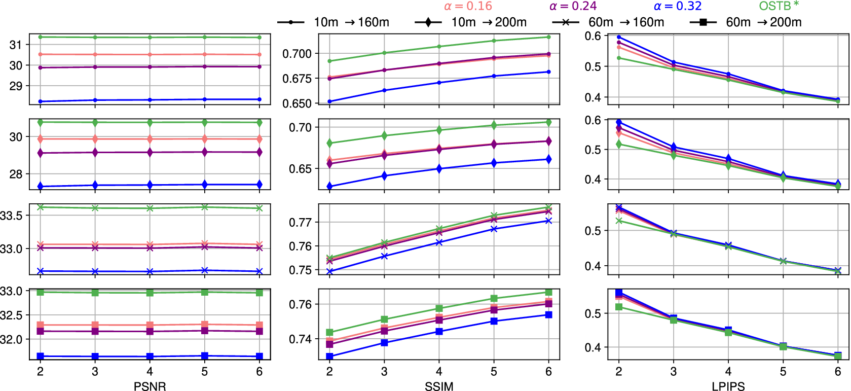
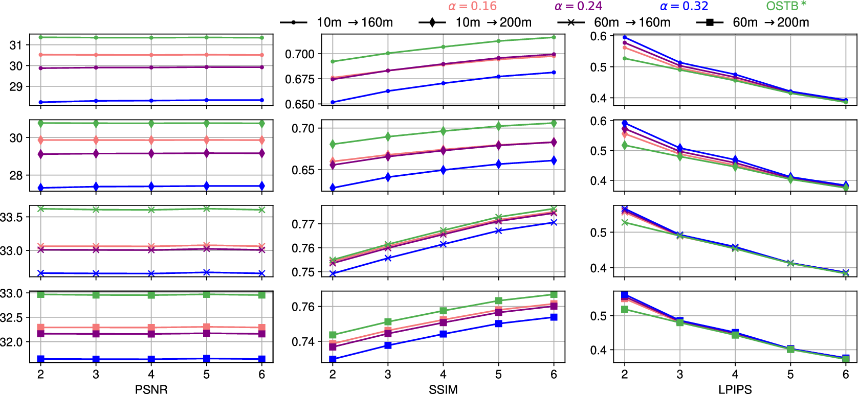
Figure 6 presents the average PSNR, SSIM, and LPIPS across the test set at different super-resolution scales. In all cross-altitude prediction scenarios, the model incorporating the 3D ETINN consistently outperforms the models without it, demonstrating the critical role of the 3D ETINN in enhancing performance.
Results for Modality Transfer Experiment.
$ x- $
 axis shows different super-resolution scales for all three subplots, and
$ y- $
axis shows different super-resolution scales for all three subplots, and
$ y- $
 axis shows the metric values (PSNR, SSIM and LPIPS metric values are shown in the three columns from left to right column accordingly). The 4 rows show the evaluation results in 4 different cross-altitude prediction scenarios:
$ 10m\to 160m $
axis shows the metric values (PSNR, SSIM and LPIPS metric values are shown in the three columns from left to right column accordingly). The 4 rows show the evaluation results in 4 different cross-altitude prediction scenarios:
$ 10m\to 160m $
 ,
$ 10m\to 200m $
,
$ 10m\to 200m $
 ,
$ 60m\to 160m $
,
$ 60m\to 160m $
 and
$ 60m\to 200m $
and
$ 60m\to 200m $
 from top to bottom row accordingly.
6.6. Additional experiment 3: ablation studies
6.6.1. Task 1
Ablation of decoder
We evaluate the performance of the proposed decoder by comparing it against other implicit neural network-based super-resolution models.
Setup
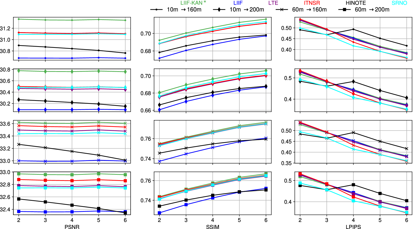
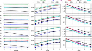
To benchmark the performance of our model, we replaced the LIIF-KAN decoder segment with the LIIF (Y Chen et al., Reference Chen, Liu and Wang2021), ITNSR (Yang et al., Reference Yang, Shen, Yue, Li, Beygelzimer, Dauphin, Liang and Vaughan2021), HiNOTE (Luo et al., Reference Luo, Qian, Yoon, Salakhutdinov, Kolter, Heller, Weller, Oliver, Scarlett and Berkenkamp2024), SRNO (Wei and Zhang, Reference Wei and Zhang2023), DIINN (QH Nguyen and Beksi, Reference Nguyen and Beksi2023), and LTE (Lee et al., Reference Lee and Jin2022) models. We also tried LTE-KAN, replacing MLP with KAN in the LTE model, similar to the modification done in LIIF-KAN. All models were trained using the same optimization procedures. Figure 7 illustrates the average PSNR and SSIM across the test set at varying super-resolution scales, with the x-axis of each plot showing the respective scales.
Ablation of decoders.
$ x- $
 axis shows different super-resolution scales for all three subplots, and
$ y- $
axis shows different super-resolution scales for all three subplots, and
$ y- $
 axis shows the metric values (PSNR, SSIM, and LPIPS metric values are shown in the three columns from left to right column accordingly). The 4 rows show the evaluation results in 4 different cross-altitude prediction scenarios:
$ 10\hskip0.42em m\to 160\hskip0.42em m $
axis shows the metric values (PSNR, SSIM, and LPIPS metric values are shown in the three columns from left to right column accordingly). The 4 rows show the evaluation results in 4 different cross-altitude prediction scenarios:
$ 10\hskip0.42em m\to 160\hskip0.42em m $
 ,
$ 10\hskip0.42em m\to 200\hskip0.42em m $
,
$ 10\hskip0.42em m\to 200\hskip0.42em m $
 ,
$ 60\hskip0.42em m\to 160\hskip0.42em m $
,
$ 60\hskip0.42em m\to 160\hskip0.42em m $
 and
$ 60\hskip0.42em m\to 200\hskip0.52em m $
and
$ 60\hskip0.42em m\to 200\hskip0.52em m $
 from top to bottom row accordingly.
Result summary
Our modified LIIF-based decoder, LIIF-KAN, consistently outperforms all other implicit super-resolution models, including the original LIIF decoder. The results show a significant performance improvement in both PSNR and SSIM, demonstrating that LIIF-KAN offers superior super-resolution capabilities compared to existing models. However, the SRNO decoder performs best among all the decoders in terms of the LPIPS metric for most of the super-resolution scales.
6.6.2. Task 2
Ablation of attention mechanisms
We assess the efficacy of the Gaussian adaptive attention in the Residual Implicit Neural blocks by comparing it with other attention mechanisms.
Setup
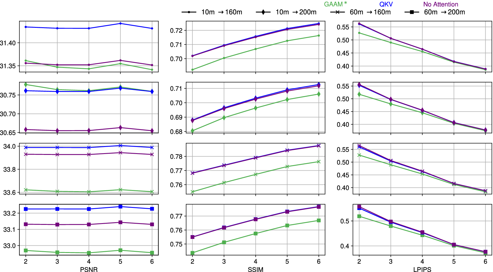
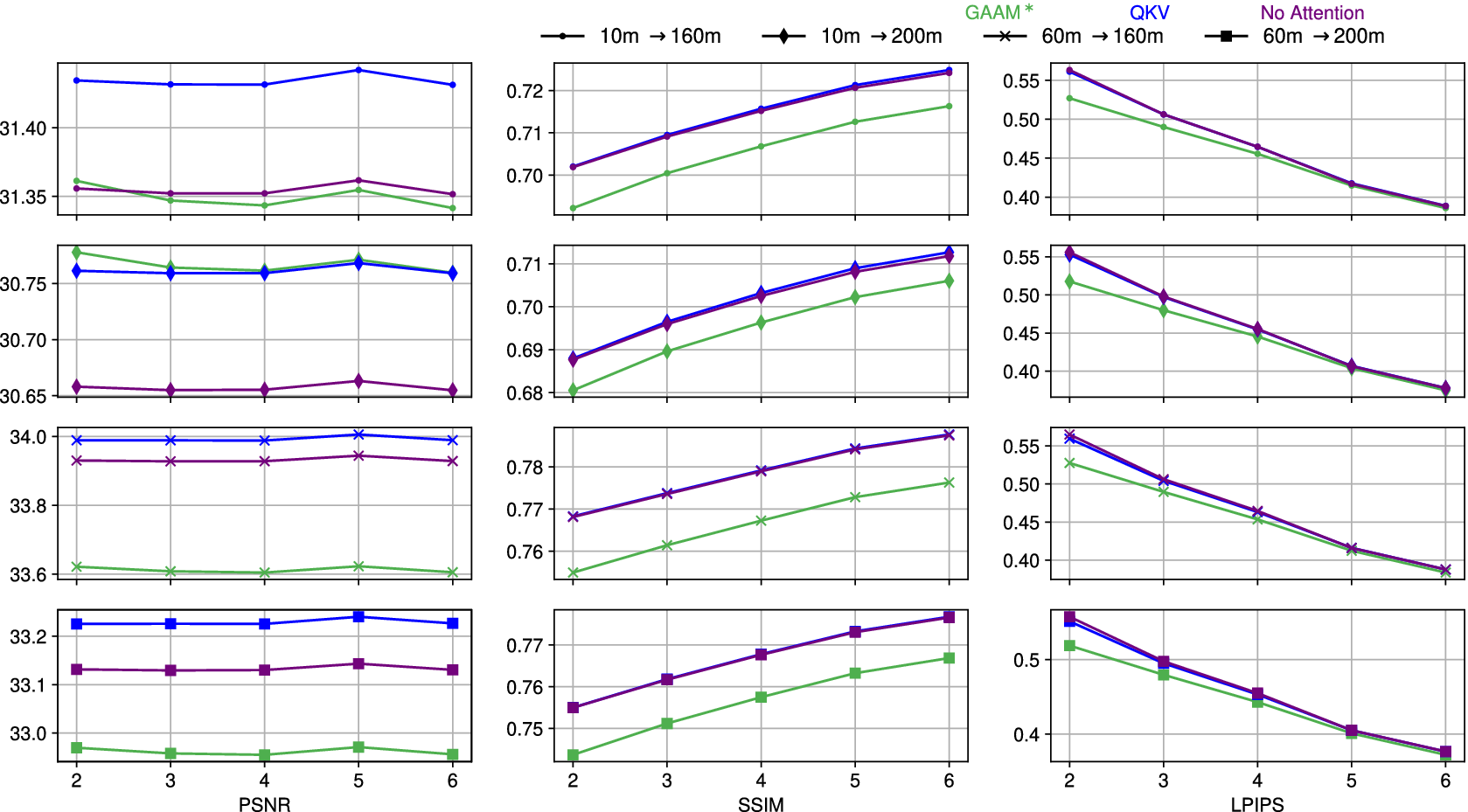
We replaced the Gaussian adaptive attention mechanism in the Residual Implicit Neural blocks with the standard Query, Key, Value (QKV) attention mechanism (Vaswani et al., Reference Vaswani, Shazeer, Parmar, Uszkoreit, Jones, Gomez, Kaiser, Polosukhin, Guyon, Luxburg, Bengio, Wallach, Fergus, Vishwanathan and Garnett2017), and also tested the performance without any attention mechanism. All models were trained following identical procedures. Figure 8 presents the results, showing the performance of each variant.
Ablation of attention mechanism.
$ x- $
 axis shows different super resolution scales for all three subplots, and
$ y- $
axis shows different super resolution scales for all three subplots, and
$ y- $
 axis shows the metric values (PSNR, SSIM, and LPIPS metric values are shown in the three columns from left to right column accordingly). The 4 rows show the evaluation results in four different cross-altitude prediction scenarios:
$ 10\hskip0.42em m\to 160\hskip0.42em m $
axis shows the metric values (PSNR, SSIM, and LPIPS metric values are shown in the three columns from left to right column accordingly). The 4 rows show the evaluation results in four different cross-altitude prediction scenarios:
$ 10\hskip0.42em m\to 160\hskip0.42em m $
 ,
$ 10\hskip0.42em m\to 200\hskip0.42em m $
,
$ 10\hskip0.42em m\to 200\hskip0.42em m $
 ,
$ 60\hskip0.42em m\to 160\hskip0.42em m $
,
$ 60\hskip0.42em m\to 160\hskip0.42em m $
 and
$ 60\hskip0.42em m\to 200\hskip0.52em m $
and
$ 60\hskip0.42em m\to 200\hskip0.52em m $
 from top to bottom row accordingly.
Result summary
The results demonstrate that our proposed method, incorporating the Gaussian adaptive attention mechanism, is outperformed by both the QKV-based attention and the version without attention in terms of PSNR and SSIM. However, it achieves lower LPIPS than its counterparts. This observation leaves us to balance among the three metrics. We have observed that our proposed model outperforms other models in all previous experiments, but it often failed to obtain low LPIPS. However, we observed that with QKV-based attention and without the attention method obtained even higher PSNR and LPIPS, but at the cost of even more suboptimal LPIPS. Also, the Gaussian adaptive attention mechanism is parameter-efficient compared to the QKV-based attention mechanism.
7. Conclusion
We have developed an innovative deep learning approach for simultaneous continuous super-resolution, data dimensionality reduction, and multi-altitude learning for climatological data. We designed a three-dimensional implicit neural network specifically for learning continuous, rather than discrete, representations of multi-altitude velocity fields used for wind farm power modeling across the continental United States. Unlike traditional multi-modal deep learning models, which handle only a limited number of modalities due to scalability issues, our three-dimensional implicit neural network is scalable to a large number of modalities. We employed two very recently proposed techniques: the Gaussian adaptive attention mechanism and the Kolmogorov–Arnold network to design our model and modify existing models. Experimental results have shown promising potential in improving wind energy assessment for electricity generation, efficient large data storage via dimensionality reduction, and extrapolation to inaccessible spatial areas. Both Gaussian adaptive attention and Kolmogorov–Arnold networks have the potential to enhance interpretability in machine learning models, making this an area for future research.
Supplementary material
The supplementary material for this article can be found at http://doi.org/10.1017/eds.2026.10043.
Acknowledgements
The authors acknowledge the use of (Google Gemini, 2025) for assistance in language editing and improving the clarity of the manuscript’s presentation. All conceptual development, technical content, analysis, and conclusions are entirely the work of the authors.
Author contribution
Conceptualization: A.B.A.Q; X.L; X.Q; B.Y. Data curation: A.B.A.Q. Formal analysis: A.B.A.Q; X.L; N.M.U; X.Q; B.Y. Funding acquisition: X.Q; B.Y. Investigation: X.L; X.Q; B.Y. Methodology: A.B.A.Q; X.L; X.Q; B.Y. Project administration: X.Q; B.Y. Resources: X.Q; B.Y. Software: A.B.A.Q; X.Q. Supervision: X.L; X.Q; B.Y. Validation: A.B.A.Q; X.L; X.Q; B.Y. Visualization: A.B.A.Q; X.L. Writing—original draft: A.B.A.Q; X.L; X.Q; B.Y. Writing - review & editing: A.B.A.Q; X.L; N.M.U; X.Q; B.Y.
Competing interests
The authors declare no competing interests.
Data availability statement
Data and code implementations can be found at https://github.com/alifbinabdulqayyum/OSTB.
Funding statement
This work was supported in part by the Department of Energy (DOE) award DE-SC0012704.








 Open access

