


I. Introduction
Two key forces animate the auto financing market: asset-backed lending (ABL) linked to the physical collateral value of vehicles (Argyle, Nadauld, Palmer, and Pratt (Reference Argyle, Nadauld, Palmer and Pratt2021), Assunçao, Benmelech, and Silva (Reference Assunçao, Benmelech and Silva2014), and Ratnadiwakara (Reference Ratnadiwakara2021)) and income-based lending (IBL) supported by a car buyer’s income (Dewatripont and Tirole (Reference Dewatripont and Tirole1994), Holmstrom and Tirole (Reference Holmstrom and Tirole1997)). In this article, we ask whether lower-income borrowers rely relatively more on ABL or IBL. A clear understanding of the roles ABL and IBL play in facilitating auto financing for economically disadvantaged consumers can provide insight into which financial innovations are likely to aid lower-income borrowers.
It is well understood that low-income consumers face restricted access to all types of financing, including mortgages and credit cards (Mills, Landau, Rodriguez, and Scally (Reference Mills, Landau, Rodriguez and Scally2022)). What is less clear, however, is whether the form of financing they do receive is more likely to be ABL or IBL. Summary market statistics do not resolve this question. For example, Fulford, Wilson, Kruse, Kalish, and Cotter (Reference Fulford, Wilson, Kruse, Kalish and Cotter2023) show that as of 2019, over the prior 6 months, 4.4% of borrowers made use of an IBL payday loan,Footnote 1 while 2.5% relied on an ABL pawn loan and 2.0% took out an ABL title loan. Auto credit has both ABL and IBL components, and we seek to understand which has greater weight in supporting the borrowing of some of the neediest Americans. Access to auto financing is particularly valuable in the U.S., where vehicle ownership is often critical for employment opportunities and mobility (Baum (Reference Baum2009), Gautier and Zenou (Reference Gautier and Zenou2010), Gurley and Bruce (Reference Gurley and Bruce2005), and Moody, Farr, Papagelis, and Keith (Reference Moody, Farr, Papagelis and Keith2021)). Recent empirical evidence from Brazil corroborates the finding that vehicular access increases formal employment rates and salaries (Van Doornik, Gomes, Schoenherr, and Skrastins (Reference Van Doornik, Gomes, Schoenherr and Skrastins2024)). Ensuring the ability of lower-income consumers to borrow to purchase cars is therefore important for a broad set of policy goals.
We make use of negative durability shocks induced by vehicle discontinuations to assess the relative use of ABL and IBL by disadvantaged auto buyers. Our main finding is that IBL is more important for lower-income borrowers. Although these borrowers have limited wages, they nonetheless rely more heavily on IBL than on ABL because they purchase assets with low liquidation values, even compared to their income. This pattern is in stark contrast to that observed in the corporate lending market, in which secured ABL is crucial for the financing of resource-constrained firms (Jimenez, Salas, and Saurina (Reference Jimenez, Salas and Saurina2006), John, Lynch, and Puri (Reference John, Lynch and Puri2003), Leeth and Scott (Reference Leeth and Scott1989), and Lian and Ma (Reference Lian and Ma2021)).
Car loan contracts do not explicitly assign weights to the ABL and IBL components of financing. ABL and IBL are thus intertwined, which presents challenges when empirically assessing the importance of IBL for auto finance across different types of borrowers. A shock to an asset’s economic durability, however, can have a differential impact on lower- and higher-income consumers in a manner that reflects their relative dependence on IBL.Footnote 2 Specifically, if lower-income borrowers rely relatively more heavily on IBL than on ABL to finance their purchases, then loan amounts for the less durable assets purchased by these borrowers (largely supported by IBL) should decrease proportionately less than the decline in collateral values. As a result, LTV (loan-to-value) ratios may be higher for less durable assets. Under these conditions, disadvantaged borrowers have somewhat less income to pledge, but they purchase assets with dramatically lower collateral values. Consequently, a reduction in durability leads to lower-income borrowers’ purchasing the asset; the asset’s financing terms then directly depend on the extent to which lower-income borrowers rely on IBL.
An implication of this argument is that if less durable assets have higher LTVs and down payments, then it must be the case that lower-income borrowers depend more heavily than higher-income borrowers on IBL. This prediction allows us to empirically assess the importance of IBL for auto lending for different kinds of borrowers.
Testing this hypothesis requires a shock to economic durability. Although cars can vary in their durability for a number of reasons (e.g., manufacturer or mileage), these sources of variation are also associated with differences along other dimensions (e.g., driving experience). We wish to isolate the pure effect of a change in economic durability by identifying shifts in durability that do not affect current vehicle quality. We utilize model and make discontinuations on existing cars as shocks to durability. We match our data to over 200 car model discontinuations and eight make discontinuations. Discontinuations may affect economic durability in two ways. First, it is likely that the physical durability of discontinued cars declines. Repair costs relative to vehicle value are of first-order importance in keeping a car on the road (Insurance Networking News (2025), and discontinuation plausibly reduces the durability of existing cars due to concerns about future parts and service expertise (Titman (Reference Titman1984)).Footnote 3 The inability to get replacement parts and increased servicing costs is frequently cited as a concern following the discontinuation of a car brand or model.Footnote 4 Second, discontinued cars may experience a loss of prestige, which should depress their current prices, which is another component of economic durability, though it is less clear whether this effect will also cause quicker value depreciation over time.
We begin our empirical analysis by showing that discontinuations reduce economic durability. Using used car prices from a broad set of wholesale auctions, we find that annual depreciation is 1.2 percentage points per year higher for discontinued vehicles. Six years after discontinuation, the effect grows to 3.3 percentage points per year. We show that after the discontinuation announcement, car values drop by about $1,068, a significant decline from the mean value of $12,493.
We then turn attention to a separate data set of loan originations to consumers and confirm that discontinued vehicles drop in value. We further find that default recoveries (the value the lender receives from the vehicle liquidation after default over the vehicle’s wholesale value at origination) decline by roughly 1.4 percentage points after discontinuations. These reduced recoveries are measured relative to the vehicles’ already lower post-discontinuation prices. These findings provide clear evidence that discontinued vehicles have reduced economic durability.
Our tests effectively compare the same model × vintage year vehicle before and after a discontinuation, while controlling for changes at the corporate parent. Discontinuation is a choice of the manufacturer but is not under direct control of other auto market participants. Buyers, sellers, and third-party financiers likely assign some probability to a possible future model discontinuation, but its actual occurrence (i.e., with certainty) must represent adverse news. Moreover, we find no evidence of increasing anticipation before the announcement; there is no observable pre-trend in vehicle values, down payment, or LTV before discontinuation. For used auto buyers, sellers, and lenders, discontinuations appear to cause an unanticipated negative shock to economic durability.
We assess the relative importance of IBL for higher- and lower-income borrowers by tracing the effects of discontinuation-driven durability shocks on down payments, LTVs, and payment-to-income (PTI) ratios. First, we show that down payments are $79 higher after discontinuations (8% relative to mean). A post-discontinuation increase in down payments only occurs if future income is sufficiently pledgeable. Lower-income consumers are forced to purchase the asset with a larger down payment, as their low future income does not allow them to borrow a large amount today. If income is not pledgeable to a meaningful degree, then the lower price of a less durable asset should lead it to be purchased with a lower down payment, which we do not observe.
Second, we show that discontinuation causes a 1.4 percentage points increase in LTV ratios. This result emerges only if lower-income borrowers make greater use of IBL. If higher-income borrowers rely more heavily on IBL (or if only ABL lending is available), by contrast, the lower liquidation values produced by a discontinuation should lead to lower LTV ratios, which we do not find. It may seem counterintuitive that discontinued vehicles have lower prices and higher down payments, yet still carry higher LTV ratios. This pattern arises when dealers apply non-proportional markups and LTV is calculated relative to book value, as is standard practice in auto lending.Footnote 5 Our study of shocks to durability enables us to examine the impact on LTVs of changes at the margin in collateral values such as those that might result from policy reforms.
In a setting that includes IBL, if lower-income borrowers are more reliant on IBL, then discontinued vehicles will be financed at lower PTI ratios. We find that to be true as well. The uniform implication of the down payment, LTV, and PTI results is that in the U.S. auto loan market income is highly pledgeable and lower-income borrowers are relatively more dependent on IBL. A model rationalizing these findings also requires that there be a constant component to dealer markups, and we show that dealer dollar margins, unlike vehicle prices, do indeed not vary with vehicle discontinuation status.
We use data on lender recoveries from vehicle repossessions to distinguish various mechanisms that link discontinuation with collateral value degradation. Although discontinued cars can physically degrade more quickly, they can also attract buyers who do not properly maintain their cars. The average proceeds from the sales of repossessed vehicles are $3,483. We show that borrowers who purchased vehicles after discontinuation have physical collateral recoveries in the event of default that are $356 lower than those of control vehicles. By contrast, borrowers who purchased vehicles that were subsequently discontinued and who defaulted after discontinuation have collateral recoveries that are $176 lower than for control cars. The latter result shows that, independent of borrower selection, discontinuation leads to worse recoveries. The difference in recoveries between these two classes of borrowers who both defaulted on loans held against discontinued cars is evidence supporting the argument that depreciation is to some extent borrower-dependent.
When IBL is a component of lending, lenders partially support the debt with a claim on the borrower’s future income. In the event of default, do auto lenders actually make recoveries aside from the vehicle repossession? We find that they do. In our defaulted sample, we show that the average cash recovery from the borrower is $1,171. This indicates that in default, physical assets and personal borrower resources supply 75% and 25%, respectively, of the total recovery proceeds.
We further test the claim that lower-income borrowers rely more on IBL by analyzing recoveries from those who bought discontinued cars and later defaulted. We find that these personal recoveries relative to the defaulted loan balance are 1.8% higher than those arising from non-discontinued cars. Discontinued cars are less expensive and are acquired by lower-income borrowers, and yet we find that their purchasers, in the event of default, supply relatively larger personal recoveries. This perhaps counterintuitive finding is rationalized by the role of IBL. Lower-income borrowers who acquire less durable assets rely more heavily on IBL; given the low collateral value of these vehicles, if default occurs, lenders seek personal recoveries.Footnote 6
Income pledgeability differs across jurisdictions and economic contexts. New developments such as open banking (Babina, Bahaj, Buchak, De Marco, Foulis, Gornall, Mazzola, and Yu (Reference Babina, Bahaj, Buchak, De Marco, Foulis, Gornall, Mazzola and Yu2024), He, Huang, and Zhou (Reference He, Huang and Zhou2023)) and the increased use of digital transactions (Agarwal and Zhang (Reference Agarwal and Zhang2020), Berg, Burg, Gombović, and Puri (Reference Berg, Burg, Gombović and Puri2020), and Boot, Hoffmann, Laeven, and Ratnovski (Reference Boot, Hoffmann, Laeven and Ratnovski2021)) can help promote IBL, and we show that this may bring special benefits to lower-income consumers. This point may be helpful in providing guidance to ensure that credit markets serve, to the maximum extent possible, to protect the relative financial access of economically disadvantaged borrowers.
II. Theoretical Framework
To illustrate the effects of a durability shock on the consumer financing of asset purchases, we provide a simple model of financing. In this section, we outline the model and describe the main results. We provide the technical details and further intuition in Section B of the Supplementary Material.
We assume that there are two types of consumers with either higher- or lower-income. Consumers can purchase more durable or less durable assets from sellers (i.e., car dealerships) who charge constant or proportional markups (or both) on sales. Both types of assets have a current period price and a residual value for the next period. Our central interest is in economic durability: we define this term to mean that assets with higher economic durability have slower rates of price depreciation over time and higher prices today. Differences in economic durability between assets may arise from variation in either physical durability or intangible quality degradation rates. Formally, we have:
Definition 1a. More durable assets have a higher ratio of residual value to current period price than less durable assets.
Definition 1b. More durable assets have a higher price than less durable assets in the current period.
We also assume that consumers prefer current over delayed consumption and thus seek to maximize their leverage. Borrowers can access financing from competitive lenders by pledging both the asset’s residual value as well as their future income. We refer to the former as ABL and the latter as IBL. ABL and IBL are both subject to limited pledgeability constraints, which govern how much financing lenders will provide. For ABL, lenders may be able to seize the collateral at some cost. For IBL, securing future income could include partial wage garnishment or bankruptcy repayment plans (Brown and Jansen (Reference Brown and Jansen2024)). In our simple setting, there is no uncertainty.
We focus on the interesting region of the parameter space by assuming that higher-income consumers can afford both goods but that lower-income consumers can only afford the less durable asset.Footnote 7 We further presume that the more durable asset is more attractive than the less durable asset to unconstrained borrowers.Footnote 8 An immediate result of these assumptions is that in equilibrium higher- (lower-) income borrowers purchase the more (less) durable good.Footnote 9
Next, we consider the implications of the model for the contrasting financing patterns of higher- and lower-income borrowers.
Result 1a. If income is sufficiently pledgeable, then lower-income borrowers purchasing the less durable asset have higher dollar down payments than higher-income borrowers purchasing the more durable asset.
Result 1b. Otherwise, the dollar down payment is lower for lower-income borrowers.
Result 2a. If lower-income borrowers are heavily dependent on IBL (implying that they rely relatively more on IBL than higher-income borrowers) and income is sufficiently pledgeable, then the LTV ratio is higher for lower-income borrowers purchasing the less durable asset than for higher-income borrowers purchasing the more durable asset.
Result 2b. Otherwise (e.g., if higher-income borrowers rely more heavily on IBL or if income is not sufficiently pledgeable), the LTV ratio is lower for lower-income borrowers.
Results 1b and 2b echo the intuitions of Rampini (Reference Rampini2019) and Hart and Moore (Reference Hart and Moore1994), which do not consider IBL. Result 1b follows from the higher price of the more durable asset not being offset one-for-one with more debt due to limited asset pledgeability and relatively low income pledgeability, leading to higher down payments for the more durable good. Result 2b is due to the more durable asset purchased by higher-income borrowers having a higher collateral value; thus, the component of the LTV ratio due solely to ABL is higher for higher-income borrowers. If these borrowers also rely more heavily on IBL than lower-income borrowers, then the IBL component of their LTV will also be higher.
Result 1a emerges only if IBL is sufficiently important. Both borrower types reduce their down payments by pledging future income, but lower-income borrowers have less income to pledge. Higher income pledgeability, holding asset values constant, reduces the down payment more for the higher-income borrower. Thus, as long as the difference in income between the two types of borrowers is sufficiently large relative to the pledgeability of income, lower-income borrowers receive smaller IBL amounts and must make larger down payments.
Result 2a emerges only if lower-income borrowers depend relatively more on IBL. Under the assumptions, less durable assets purchased by lower-income borrowers have two features: they are purchased with less debt in dollar terms and they have lower residual values. A comparison of the LTV ratios of more durable and less durable assets therefore depends on the relative strength of these two effects. If lower-income borrowers rely heavily on IBL (implying that they rely more on IBL than do higher-income borrowers), then a greater proportion of their borrowing is based on future income rather than on residual asset value. As a result, as long as income is also sufficiently pledgeable, then lower-income borrowers carry a high level of debt (largely supported by IBL) relative to the low collateral value of their less durable asset.
The model also has implications for borrowers’ payment-to-income (PTI) ratios.
Result 3a. If lower-income borrowers rely relatively more on IBL than higher-income borrowers, then the PTI ratio is lower for lower-income borrowers purchasing the less durable asset than it is for higher-income borrowers purchasing the more durable asset.
Result 3b. Otherwise, the PTI ratio is higher for lower-income borrowers.
Result 3a arises from the fact that the promised payment for the less durable good depends at least in part on its future residual value. If this future residual value for the less durable asset is very low, which is the case when the lower-income borrower is highly dependent on IBL, then the future payment must also be low.
There are parameters that simultaneously satisfy the conditions of Results 1a, 2a, and 3a, as well as the other model assumptions. Thus, the following implications arise from the model:
Model Implications. If down payments are non-negative,
-
a) the down payment is higher for the less durable asset, b) the LTV ratio is higher for the less durable asset, and c) the PTI ratio is lower for the less durable asset, then
-
i) income must be sufficiently pledgeable, ii) lower-income borrowers must rely relatively more heavily than higher-income borrowers on IBL and iii) there must be a constant component of the markup.
Figure B.1 in the Supplementary Material presents a graphical illustration of the results. There are six regions that describe the down payment, LTV, and PTI for the less durable asset purchased by the lower-income consumer relative to the more durable asset purchased by the higher-income consumer, with the regions defined by their relationship to three cutoff conditions. First, if the pledgeability of income is above the dark red line, then higher-income borrowers rely more on their future income to cover their obligations and lower-income borrowers make larger down payments. Second, if the durability of the less durable asset is below (i.e., to the left of) the blue curve (and income is sufficiently pledgeable), then lower-income consumers borrow a high level of debt relative to the low collateral value of their asset and have higher LTVs. Third, if the durability of the less durable asset is below (i.e., to the left of) the purple line, then lower-income borrowers have lower PTI ratios because they cannot borrow much against the low future value of their asset.
Thus, if lower-income borrowers have higher down payments and LTVs and lower PTIs, then income pledgeability must be high and the economic durability of the lower-income asset must be low, with the parameter values residing in light green region I.
Measuring ABL and IBL
The model implications allow us to assess the relative dependence of higher- and lower-income borrowers on IBL through an analysis relating durability to down payments, LTVs and PTIs. A natural direct alternative would be to measure ABL, perhaps by calculating collateral values, and to view any non-ABL financing as arising from IBL. One could then simply compare in the cross section the relative use of ABL and IBL by higher- and lower-income borrowers.
The central challenge with this direct approach is that the assets purchased by higher- and lower-income borrowers likely vary significantly in the amenities and features they offer. Consequently, these assets may be sold in different markets and financed by different lenders. In other words, financing choices by consumers of heterogeneous income levels may be driven by complex unobserved variation across multiple characteristics of the assets they purchase. As described in Section IV, we instead focus on vehicle discontinuations that generate a pure shock to durability that holds fixed other asset characteristics. We are thereby able to isolate the impact of durability and to trace the effects of a shift in ABL. As in the direct method, we then infer the relative weight of ABL versus IBL by considering the collateral value of the asset relative to the amount of financing. Further, our study of shocks to durability enables us to examine the impact on LTVs of changes at the margin in collateral values, such as those that might result from policy reforms.Footnote 10
III. Data
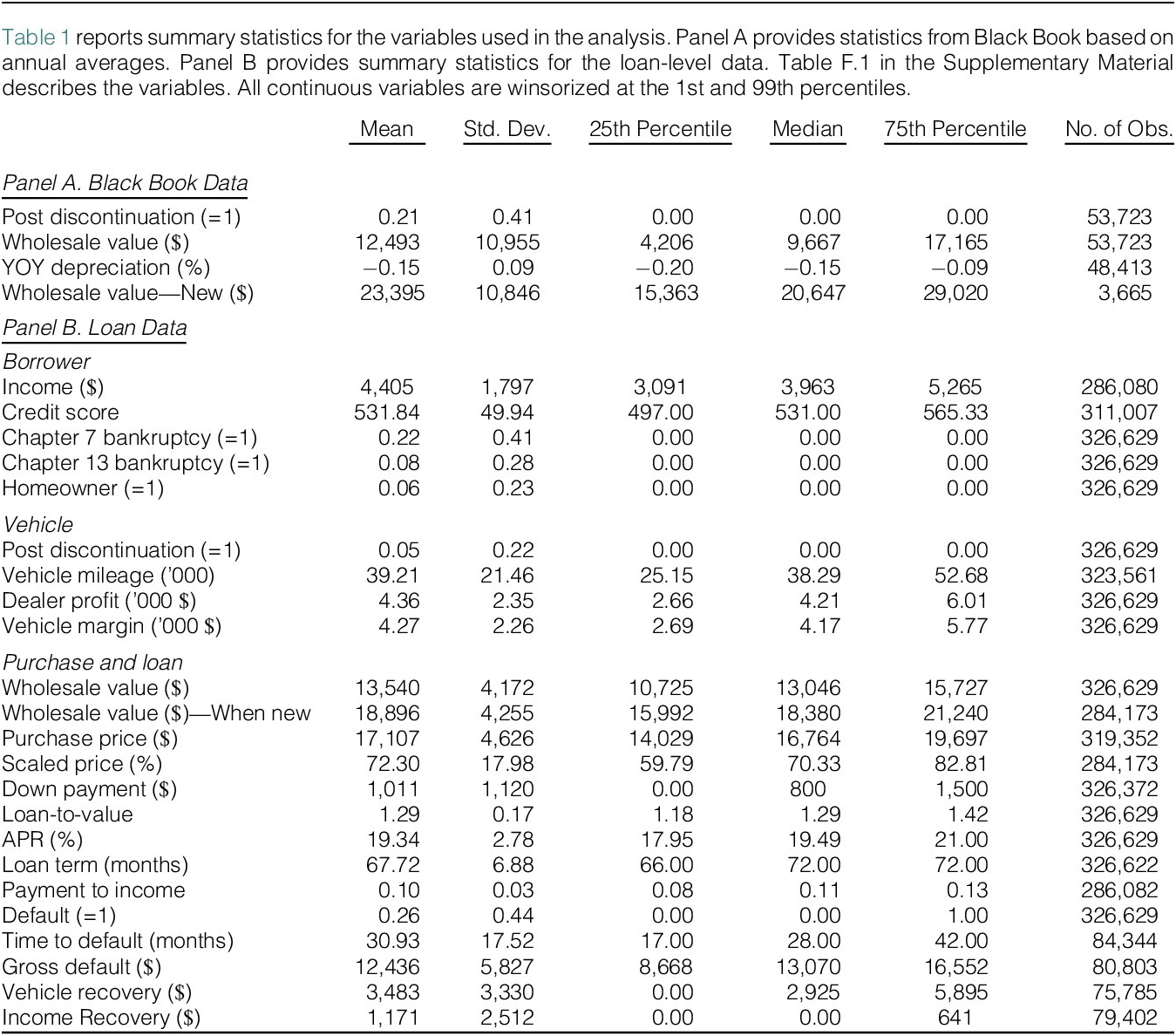
To explore the role of asset durability on consumer financing, we use two data sets. The first data set, supplied by Black Book, provides panel information on 746 vehicle make-models on wholesale values from car auctions of used vehicles.Footnote 11 In total, this represents 5085 make-model-year observations spanning 2001–2020 model years.Footnote 12 The wholesale values that we use in our analysis cover the period from May 2001 to October 2020 and we compute annual wholesale values by averaging across monthly observations. We use these average wholesale values to calculate year-over-year (YOY) depreciation rates, which we define as the difference between this year’s wholesale value and last year’s wholesale value, with the difference scaled by the wholesale value last year. Summary statistics are reported in Panel A of Table 1.

The second data set, the loan data, describes loan terms offered by a large independent automotive indirect-finance company.Footnote 13 The data include all loans purchased by the firm in 44 states between 1992 and 2021. In total, we observe key features of 326,629 loans that were originated at 4,622 dealerships located in 2,077 U.S. ZIP codes as described in Panel B of Table 1.Footnote 14 The lender is one of the top 20 auto finance companies in the United States. Auto buyers can either secure a loan directly from a bank or credit union or finance indirectly through an auto dealership, which then sells the loan to a third-party lender. Our lender originates loans via indirect financing, which accounts for 83% of auto lending in the U.S. (Grunewald, Lanning, Low, and Salz (Reference Grunewald, Lanning, Low and Salz2023)).
The breadth and detail of our loan data distinguish our study from previous work. More specifically, we observe loan characteristics (e.g., purchase price and down payment) that are typically unavailable in aggregate data. For example, Experian Autocount data do not measure down payments and sale prices, limiting the construction of collateral measures.Footnote 15
Panel B of Table 1 presents summary statistics from loan data of the buyer, loan, and vehicle characteristics that were observable to the dealer at the time of origination for all loans in our sample, where we observe complete origination data. In our sample, the median vehicle is 2 years old and has approximately 38,000 miles when sold. The median vehicle has a value of $13,046, and the median down payment is $800 (roughly 6% of the vehicle’s value). We find average dealer margins of $4,273 (roughly 25% of the purchase price). The median loan in our sample has a term of 72 months (6 years) and an APR of approximately 19.5%. The high APR reflects the fact that the borrowers in the sample are subprime—the median reported credit score is approximately 530, with approximately 30% of borrowers having a reported bankruptcy (chapter 7 or 13) within 7 years of loan origination. The median monthly income is $3963, so our income comparisons across borrowers are within a set of resource-constrained consumers.
IV. Discontinuations
A. Background
To causally identify the impact of economic durability on financing, we require a source of exogenous variation in asset economic durability. Moreover, to separate any general effect of durability from other technological shocks in the time series (e.g., financial engineering or digital processing of applications), we require a shock that affects only some vehicles, but that still allows for controls for vehicle age, manufacturer, model, and the year the vehicle was sold. Ideally, we would randomly assign different economic durability to similar vehicles. While this may not be feasible, we can take advantage of shocks to existing vehicles that affect their current and future resale values. Specifically, we utilize discontinuation of vehicles’ makes and models as a source of exogenous variation in vehicle economic durability in our data.
This shock does not affect the current quality of a used car because no component of the car changes. In this sense, the shock to quality is only forward-looking, although it may be reflected in current prices. Before discontinuation, the car is made in the same factories with the same materials. Moreover, by comparing car prices prior to discontinuation to the same model and year of car post-discontinuation, we can hold constant the car quality and use vehicles that were not shocked to control for the but-for depreciation curve and other time-varying attributes of the market.
One concern with this shock is that the decision to discontinue a make and model of car by the car manufacturer is an endogenous decision and there are many reasons a manufacturer may choose to do so. For instance, a car manufacturer may choose to cut less profitable models during times of financial distress. However, in our specifications we can directly control for the parent car company and thus can compare cars of similar quality within the same car manufacturing family. Thus, any effect on durability due to potential future bankruptcy, as noted in Titman (Reference Titman1984) and shown to be empirically important in Titman and Wessels (Reference Titman and Wessels1988) and Hortaçsu, Matvos, Syverson, and Venkataraman (Reference Hortaçsu, Matvos, Syverson and Venkataraman2013) among others, should affect all cars made by that manufacturer. Additionally, in several cases, the discontinuation happened when the auto manufacturer was not in financial distress. Moreover, by comparing pre-trends of the vehicles, we can plausibly detect any movements in the resale or depreciation value of the vehicles prior to the shock.
B. Discontinuation Shocks
In the last 25 years, 825 car models have been discontinued. Among the 825 discontinued models, we identify 208 instances in which the manufacturer decides to maintain the make of the car (e.g., Chevrolet) but discontinues a specific model (e.g., Chevrolet Monte Carlo), and the model appears in our loan data.Footnote 16 We supplement these model discontinuations with eight discontinuations of major U.S. car brands (i.e., makes) during our sample period. A list of discontinued models, discontinued makes, and discontinuation years is provided in Tables F.2 and F.3 in the Supplementary Material.
C. Empirical Method
We use a difference-in-difference (DiD) approach to test the effect of our shock to depreciation. Specifically, for a transaction $ i $
, of model
$ i $
, of model $ j $
of vintage
$ j $
of vintage $ v $
, with parent
$ v $
, with parent $ p $
and dealer
$ p $
and dealer $ d $
, during period
$ d $
, during period $ t $
, we estimate the following regression:
$ t $
, we estimate the following regression:
 $$ {Y}_{i,j,d,t,v,p}={\tau}_t+{\iota}_{j,v}+{\xi}_d+{\pi}_{p,t}+\beta {X}_{i,j,d}+{\phi}_{j,t}{\mathrm{Treated}}_{j,t}+{\unicode{x025B}}_{i,j,d,t}, $$
where $ Y $
is an outcome such as vehicle price or financing term,
$ Y $
is an outcome such as vehicle price or financing term, $ \tau $
is a transaction year fixed effect,
$ \tau $
is a transaction year fixed effect, $ \iota $
is a car model × vintage year fixed effect,
$ \iota $
is a car model × vintage year fixed effect, $ \xi $
is a dealer fixed effect,
$ \xi $
is a dealer fixed effect, $ X $
are a series of vehicle, borrower, and dealer controls, and Treated is an indicator if the make of model
$ X $
are a series of vehicle, borrower, and dealer controls, and Treated is an indicator if the make of model $ j $
has been discontinued prior to time
$ j $
has been discontinued prior to time $ t $
. Thus, in the cross section, we are comparing cars within the same period, absorbing any non-time varying attributes related to the specific model, and dealer, as well as any linear effects of vehicle age. In addition, we also include fixed effects for the interactions of the parent company of the car maker × transaction year fixed effects (
$ t $
. Thus, in the cross section, we are comparing cars within the same period, absorbing any non-time varying attributes related to the specific model, and dealer, as well as any linear effects of vehicle age. In addition, we also include fixed effects for the interactions of the parent company of the car maker × transaction year fixed effects ( $ {\pi}_{p,t} $
). Thus, we also absorb any effects related to the financial condition of the parent company at the time of the transaction. Importantly, this isolates general effects that would apply to all makes of a given parent company (e.g., GM during the 2008–2009 Global Financial Crisis). In all specifications, we cluster by make.Footnote
17
$ {\pi}_{p,t} $
). Thus, we also absorb any effects related to the financial condition of the parent company at the time of the transaction. Importantly, this isolates general effects that would apply to all makes of a given parent company (e.g., GM during the 2008–2009 Global Financial Crisis). In all specifications, we cluster by make.Footnote
17
V. Results
A. Discontinuation Shock and Economic Durability
We use the discontinuation of models and brands described in Section IV as a shock to economic durability. Parts availability and servicing expertise for discontinued vehicles are likely to degrade more quickly than for other vehicles. There may also be a loss of prestige that leads to lower current prices. From the perspective of the theoretical framework described in Section II, this suggests that discontinuation may be viewed as a shock that reduces the economic durability of a car.
We begin by using the Black Book data to empirically assess the impact of discontinuation on economic durability. Definition 1a in Section II requires that more durable assets have a higher ratio of residual value to current period price (i.e., lower YOY depreciation), so if discontinuation reduces durability, then it should increase the rate of depreciation. We test this implication by estimating equation (1) and regressing a vehicle’s YOY depreciation on a post-discontinuation indicator, model × vintage year fixed effects, and corporate parent × contract year fixed effects. Our use of model × vintage year fixed effects allows us to contrast vehicles of the exact same model and vintage year before and after discontinuation. Corporate parent × contract year fixed effects remove any impacts that influenced the corporate parent. It is plausible that corporations that discontinue a make or model may differ from those that do not. For example, it could be that corporate parents that discontinue a make or model may have weaker balance sheets and may therefore be less capable of guaranteeing future warranties. The corporate parent-contract year fixed effects control for any impacts of this kind. Taken together, this complement of fixed effects isolates the impact of discontinuation itself on the specific model that will no longer be manufactured.
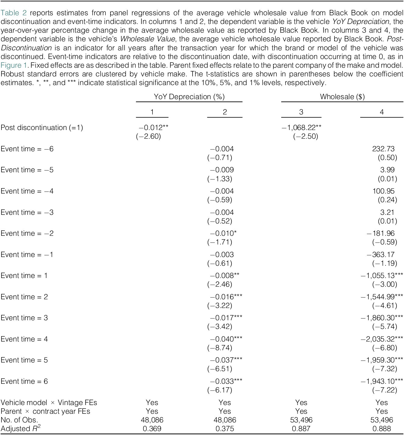
We find (shown in column 1 of Table 2) that discontinued vehicles depreciate by an additional −1.2% ( $ t $
-stat = −2.60) per year. This is a meaningful effect relative to the average depreciation rate of −15%. This finding of more severe depreciation after discontinuation is consistent with the claim that discontinuation reduces economic durability. In the second column of Table 2, we show that vehicles experience sustained rates of elevated annual depreciation after discontinuation, ranging from −0.8% (
$ t $
-stat = −2.60) per year. This is a meaningful effect relative to the average depreciation rate of −15%. This finding of more severe depreciation after discontinuation is consistent with the claim that discontinuation reduces economic durability. In the second column of Table 2, we show that vehicles experience sustained rates of elevated annual depreciation after discontinuation, ranging from −0.8% ( $ t $
-stat = −2.46) in the first year after discontinuation to −3.3% (
$ t $
-stat = −2.46) in the first year after discontinuation to −3.3% ( $ t $
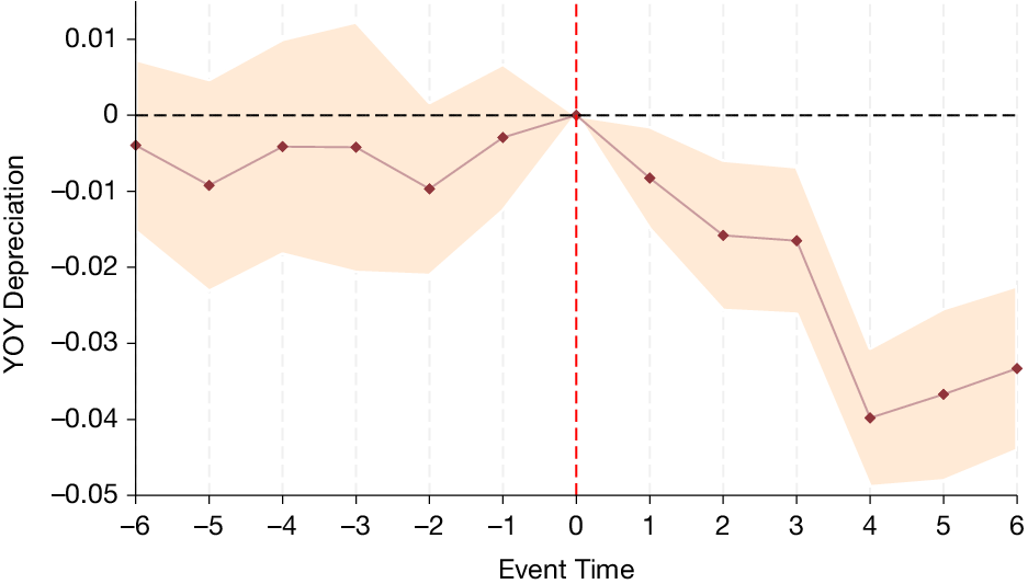
-stat = −6.17) in the sixth post-discontinuation year. These results are illustrated graphically in Figure 1.
$ t $
-stat = −6.17) in the sixth post-discontinuation year. These results are illustrated graphically in Figure 1.

Figure 1 presents differences in the year-over-year (YoY) depreciation across vehicles (models and makes) that were discontinued and those that were not. The plot displays the regression coefficients for timing indicators around the year the model was discontinued (discontinuation year = 0). The dependent variable is the percentage change in the average annual wholesale value of the vehicle as reported by Black Book. Included fixed effects are Make/Model $ \times $
Vintage Year and Contract Year
$ \times $
Vintage Year and Contract Year $ \times $
Parent Company.
$ \times $
Parent Company.

The initial increase in depreciation in the first year after discontinuation likely reflects both the impaired physical durability of discontinued vehicles and the stigma associated with these cars. The fact that the rate of depreciation is greater in subsequent years, however, probably largely arises from a decrease in physical durability, as it seems unlikely that the loss of prestige for discontinued cars would increase over time as a fraction of overall value.
The second key feature of less durable assets, which is highlighted in Definition 1b in Section II, is that they have lower prices. We show in the third column of Table 2 that discontinuation leads to a $1,068.2 drop ( $ t $
-stat = −2.50) in vehicle wholesale values. This is a meaningful decrease compared to the average wholesale value of $12,493. As shown in the fourth column of Table 2, the price effect is substantial in the first year after discontinuation (coefficient = −1055.1 and
$ t $
-stat = −2.50) in vehicle wholesale values. This is a meaningful decrease compared to the average wholesale value of $12,493. As shown in the fourth column of Table 2, the price effect is substantial in the first year after discontinuation (coefficient = −1055.1 and $ t $
-stat = −3.00) and is larger in subsequent years.Footnote
18 Table 2 makes clear that discontinued vehicles are less economically durable, exhibiting both increased rates of annual depreciation and lower prices.
$ t $
-stat = −3.00) and is larger in subsequent years.Footnote
18 Table 2 makes clear that discontinued vehicles are less economically durable, exhibiting both increased rates of annual depreciation and lower prices.
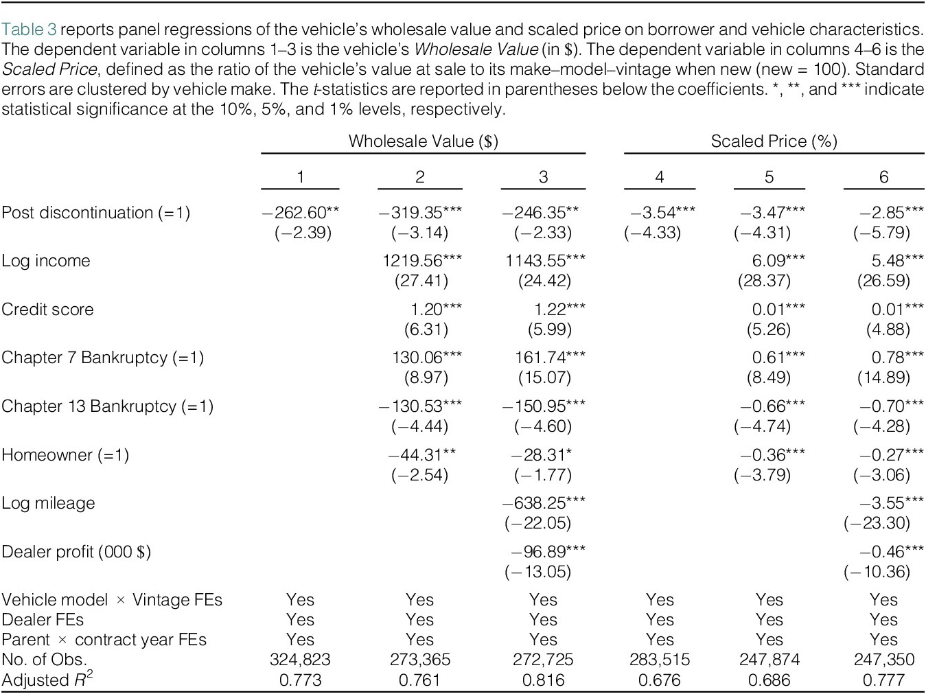
Next, we examine the impact of discontinuation on vehicles in our loan data. These data describe sales of individual vehicles, so they can be used to analyze prices, but are not in the form of a panel that allows for the calculation of annual depreciation. We regress the vehicle wholesale value on a post-discontinuation indicator, model × vintage year fixed effects, dealer fixed effects, and corporate parent × contract year fixed effects, which we refer to as the standard set of fixed effects. We find (shown in column 1 of Table 3) that discontinued vehicles experience a change in wholesale value of -$262.6 ( $ t $
-stat = −2.39). The negative sign of this effect is consistent with the results in Table 2. The magnitude of the drop is smaller than for the vehicles in the Black Book sample, which may arise from the fact that the loan data are generated from subprime borrowers sales, whereas the Black Book data describe a broad cross section of vehicles.Footnote
19
$ t $
-stat = −2.39). The negative sign of this effect is consistent with the results in Table 2. The magnitude of the drop is smaller than for the vehicles in the Black Book sample, which may arise from the fact that the loan data are generated from subprime borrowers sales, whereas the Black Book data describe a broad cross section of vehicles.Footnote
19

Including controls for borrower income and credit score, indicators for prior borrower Chapter 7 or Chapter 13 bankruptcy filings and an indicator for borrower homeowner status leave the qualitative finding unchanged, as shown in the second column of Table 3. Including a control for vehicle mileage and dealer profit yields the result that discontinuation reduces the wholesale value by $246.35 ( $ t $
-stat = −2.33).
$ t $
-stat = −2.33).
We also measure vehicle value using the scaled price, defined as the wholesale value divided by the average wholesale value of the same model and vintage when new. We show in the fourth column of Table 3 that the scaled price is 3.54 percentage points lower ( $ t $
-stat = −4.33) post-discontinuation. The results from the specifications including borrower, vehicle mileage, and dealer profit controls in the scaled price regressions support the conclusion that discontinuation reduces vehicle value, as shown in columns 5 and 6 of Table 3.
$ t $
-stat = −4.33) post-discontinuation. The results from the specifications including borrower, vehicle mileage, and dealer profit controls in the scaled price regressions support the conclusion that discontinuation reduces vehicle value, as shown in columns 5 and 6 of Table 3.
As an additional test for whether discontinuation can be viewed as a negative durability shock, we study the recovery percent of a vehicle, which we define to be the value the lender receives from the vehicle’s liquidation after default divided by the vehicle’s wholesale value at origination. We regress the recovery percent on the post-discontinuation dummy and the standard fixed effects. We note here for clarity that we assign the post-discontinuation indicator to a vehicle if it is purchased after discontinuation. As shown in Tables 2 and 3, these vehicles have lower current period prices when purchased. In the present test, we explore whether their future recovery values are lower, as a fraction of their already reduced prices, relative to other vehicles.
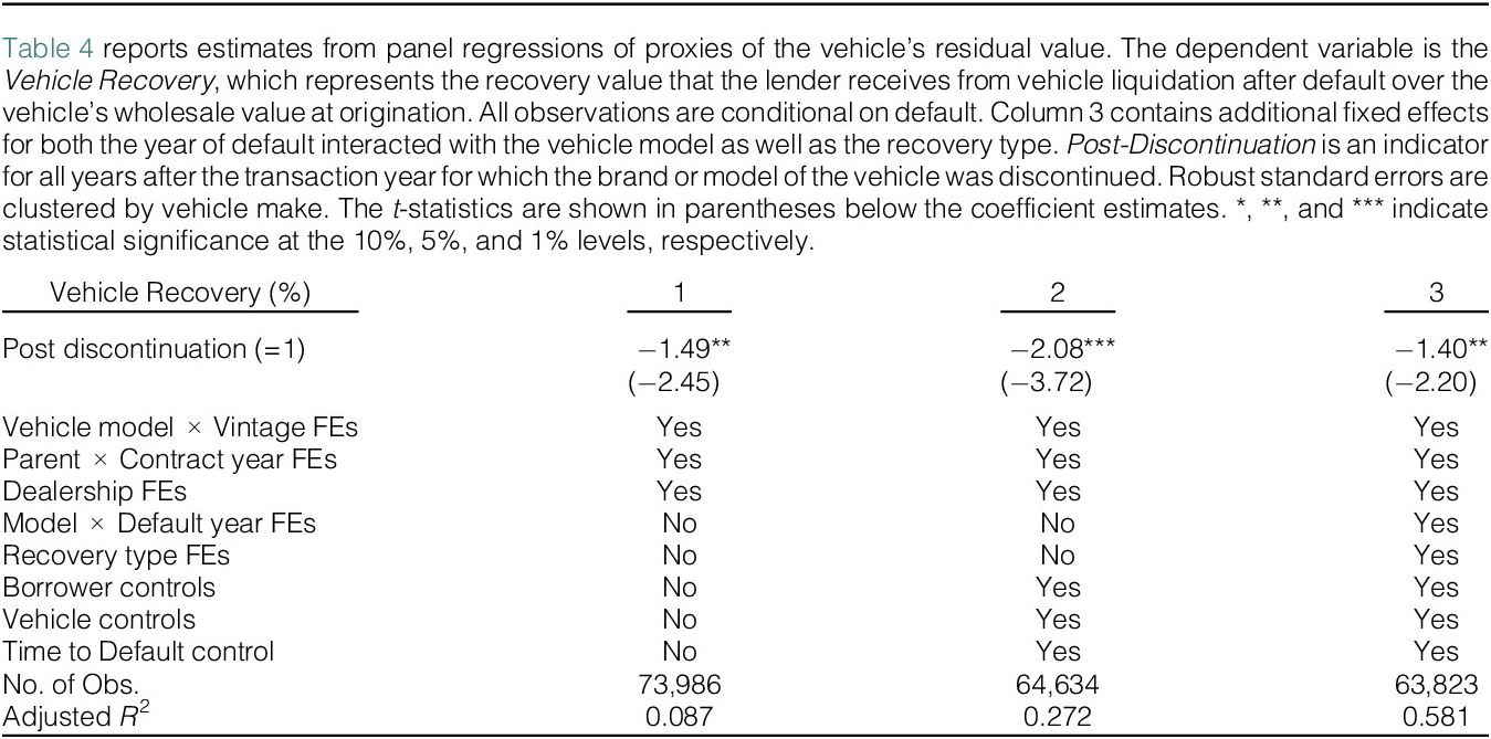
We find, as shown in the first column of Table 4, that the recovery percent is 1.49 percentage points lower ( $ t $
-stat = −2.45) for post-discontinuation vehicles. This drop may be compared to the average recovery ratio of 28%. In the second column of Table 4, we show that including borrower, vehicle mileage, and dealer profit controls as well as a control for the time to default yields a coefficient of −2.08 percentage points (
$ t $
-stat = −2.45) for post-discontinuation vehicles. This drop may be compared to the average recovery ratio of 28%. In the second column of Table 4, we show that including borrower, vehicle mileage, and dealer profit controls as well as a control for the time to default yields a coefficient of −2.08 percentage points ( $ t $
-stat = −3.72) on post-discontinuation. Including an additional fixed effect for the model × year of default as well as controlling for the recovery type results in an estimated coefficient of −1.40 percentage points (
$ t $
-stat = −3.72) on post-discontinuation. Including an additional fixed effect for the model × year of default as well as controlling for the recovery type results in an estimated coefficient of −1.40 percentage points ( $ t $
-stat = −2.20), as shown in the third column of Table 4. These results support the general conclusion that discontinued vehicles have lower residual values, even when viewing these residual values as a fraction of their lower prices at the time of purchase.
$ t $
-stat = −2.20), as shown in the third column of Table 4. These results support the general conclusion that discontinued vehicles have lower residual values, even when viewing these residual values as a fraction of their lower prices at the time of purchase.

Tables 2, 3, and 4 make clear that the discontinuation shock reduces economic durability, as described in Definition 1. Discontinued vehicles have higher depreciation rates, lower prices, and lower residual values, and consequently we view them as less durable assets for the purpose of testing the theoretical predictions outlined in Section II.
B. Durability and Consumer Income
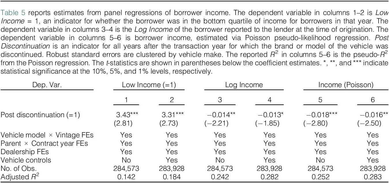
A direct implication from the assumptions of the theoretical framework presented in Section II is that higher-income borrowers will purchase more durable assets. The basic intuition is that more economically durable assets are attractive but expensive. We test this prediction by regressing an indicator for whether a borrower had a bottom-quartile income relative to all borrowers in that year on the post-discontinuation dummy and the standard fixed effects. We find, as shown in the first column of Table 5, that discontinuation increases the probability that the purchaser is in the bottom income quartile by 3.43 percentage points ( $ t $
-stat = 2.81). This represents a large 13.7% increase in the probability that the buyer is lower-income. This finding is consistent with the implication that lower-income borrowers are more likely to buy less durable discontinued vehicles. Including controls yields a similar conclusion, as shown in the second column of Table 5. A regression of the log of borrower income on discontinuation yields a coefficient of −0.014 (
$ t $
-stat = 2.81). This represents a large 13.7% increase in the probability that the buyer is lower-income. This finding is consistent with the implication that lower-income borrowers are more likely to buy less durable discontinued vehicles. Including controls yields a similar conclusion, as shown in the second column of Table 5. A regression of the log of borrower income on discontinuation yields a coefficient of −0.014 ( $ t $
-stat = −2.21), as displayed in the third column of Table 5; the negative impact of discontinuation on income is evidently strongest in shifting buyers into the lowest quartile. This result is robust to controlling vehicle mileage and dealer profits and also emerges in specifications using Poisson regressions as suggested by Silva and Tenreyro (Reference Silva and Tenreyro2006) and Cohn, Liu, and Wardlaw (Reference Cohn, Liu and Wardlaw2022), as shown in columns 4–6 of Table 5. Discontinued vehicles are purchased by lower-income borrowers, and the effect is especially pronounced for borrowers in the bottom-income quartile.
$ t $
-stat = −2.21), as displayed in the third column of Table 5; the negative impact of discontinuation on income is evidently strongest in shifting buyers into the lowest quartile. This result is robust to controlling vehicle mileage and dealer profits and also emerges in specifications using Poisson regressions as suggested by Silva and Tenreyro (Reference Silva and Tenreyro2006) and Cohn, Liu, and Wardlaw (Reference Cohn, Liu and Wardlaw2022), as shown in columns 4–6 of Table 5. Discontinued vehicles are purchased by lower-income borrowers, and the effect is especially pronounced for borrowers in the bottom-income quartile.

C. Durability and Down Payments
The results described in Section V.A serve to validate the use of discontinuation as a shock to economic durability, while the results in Section V.B support our assumptions for the relationship between a reduction in durability and borrower income.Footnote 20
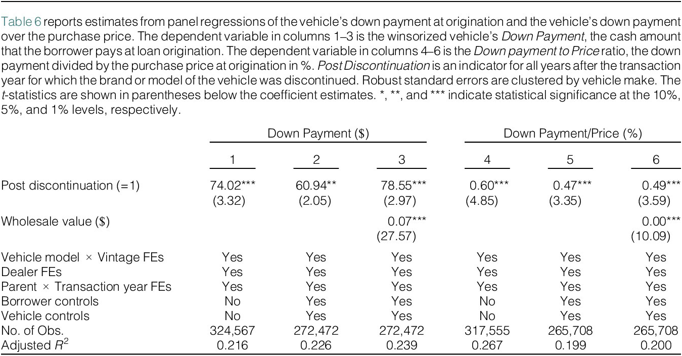
The model offers conflicting predictions for the impact of economic durability on the dollar value of the borrower’s down payment (i.e., the cash amount paid by the borrower on the transaction date). When income pledgeability is low, more durable assets require larger down payments (Result 1b); while when income pledgeability is sufficiently high, borrowers purchase less durable assets with larger down payments (Result 1a).
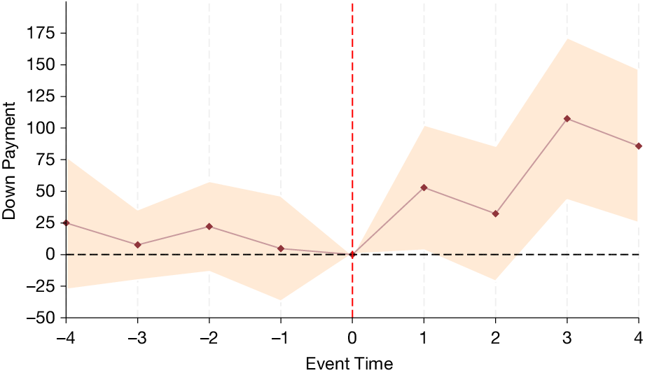
We regress the down payment on the post-discontinuation indicator and the standard fixed effects. We find that discontinuation leads to larger down payments, as shown in the first column of Table 6. Consistent with the implication in the model when income is sufficiently pledgeable, borrowers supply an additional $74.02 ( $ t $
-stat = 3.32) in down payments when purchasing less durable discontinued vehicles. As shown in Figure 2, down payments climb significantly after discontinuation and do not exhibit any apparent pre-trend.
$ t $
-stat = 3.32) in down payments when purchasing less durable discontinued vehicles. As shown in Figure 2, down payments climb significantly after discontinuation and do not exhibit any apparent pre-trend.

Figure 2 presents differences in the down payments across vehicles (models and makes) that were discontinued and those that were not. The plot is the regression coefficients for timing indicators around the year the model was discontinued (discontinuation year = 0). The dependent variable is the down payment for the vehicle. Included fixed effects are Make/Model $ \times $
Vintage Year, Dealership, and Contract Year
$ \times $
Vintage Year, Dealership, and Contract Year $ \times $
Parent Company.
$ \times $
Parent Company.

This down payment result is particularly surprising from the perspective of a model with only asset-based collateral (i.e., if income was not pledgeable). We showed in Table 3 that discontinued vehicles are less expensive. This fact, along with the limited pledgeability of collateral emphasized in asset-backed models of lending, should lead discontinued autos to require lower down payments. Moreover, we demonstrate in Table 5 that these vehicles are purchased by lower-income borrowers who presumably have less cash on hand for a down payment. Despite these two compelling intuitions for a prediction that there will be lower down payments for less durable assets, we find the opposite. This finding in the context of the model shows that IBL is a relatively important feature of auto lending. Given that lower-income consumers have smaller future incomes against which to borrow, lower-income purchasers of less durable assets need to provide larger down payments to close the transactions.Footnote 21
The positive impact of discontinuation on down payments continues to hold when controlling for borrower and vehicle characteristics, as detailed in the second column of Table 6. We show in the third column of Table 6 that in the cross section more expensive vehicles with elevated book values generally require higher down payments. There are, however, many unobserved differences between vehicles of different prices. Our result that discontinuation shocks lead to higher down payments on vehicles of specific model × vintage years is somewhat stronger when controlling for this vehicle book value effect, as is displayed in the third column. We also find, as described in columns 4–6 of Table 6, that after discontinuation down payments increase as a fraction of price.
The higher down payments for less durable assets that we find indicate that the empirically relevant regions of Figure B.1 in the Supplementary Material are restricted to region I (light green), region II (orange), or region III (dark pink). Only for the high levels of income pledgeability that hold in those regions will lower-income borrowers make the higher down payments that we observe. The other regions are incompatible with the down payment results in Table 6.
D. Durability and LTV Ratios
In this section, we consider the implications of the model for the LTV ratio. Specifically, in our model, when IBL is relatively unimportant for lower-income borrowers, LTV increases with durability (Result 2b), but when IBL is relatively important for lower-income borrowers, LTV decreases with durability (Result 2a).
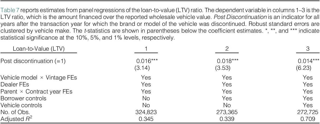
We define the LTV as the ratio of the loan balance to the wholesale value of the auto at the time of origination. We regress LTV on the post-discontinuation indicator and the standard fixed effects, and find a positive and significant coefficient of 0.016 ( $ t $
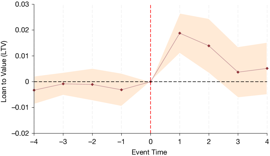
-stat = 3.14), as displayed in the first column of Table 7. This result shows that a discontinuation shock reducing vehicle durability leads to higher LTV ratios, which, as we describe in Section II, arises only in the model when lower-income borrowers are highly dependent on IBL. Figure 3 shows that LTV ratios exhibit no pre-trend before discontinuations and are higher afterward.
$ t $
-stat = 3.14), as displayed in the first column of Table 7. This result shows that a discontinuation shock reducing vehicle durability leads to higher LTV ratios, which, as we describe in Section II, arises only in the model when lower-income borrowers are highly dependent on IBL. Figure 3 shows that LTV ratios exhibit no pre-trend before discontinuations and are higher afterward.

Figure 3 presents differences in the loan-to-value (LTV) across vehicles (models and makes) that were discontinued and those that were not. The plot is the regression coefficients for timing indicators around the year the model was discontinued (discontinuation year = 0). The dependent variable is the loan amount divided by the reported vehicle value to the lender for the vehicle. Included fixed effects are Make/Model $ \times $
Vintage Year, Dealership, and Contract Year
$ \times $
Vintage Year, Dealership, and Contract Year $ \times $
Parent Company.
$ \times $
Parent Company.

It is a general and robust feature of models of asset-backed financing that LTV increases with durability (Hart and Moore (Reference Hart and Moore1994)). When the asset constitutes the entire collateral, as in a model without IBL, more durable assets with higher liquidation values support larger loans relative to current values. We also find this implication in our model when IBL is relatively less important for lower-income borrowers (these are regions II, III, IV, and V in Figure B.1 in the Supplementary Material). Our finding to the contrary indicates that in the auto loan market, IBL must play a meaningful role and that it is especially important for lower-income borrowers. Our model describes a setting in which borrowers can rely on their future income to purchase assets. Lower-income borrowers, in particular, use their future income to purchase less durable assets. If the price of the less durable asset is relatively low, then lower-income borrowers will purchase it with a relatively high debt ratio, as the debt is secured by their income, not just by the physical collateral. This mechanism in the model is consistent with the finding that LTV increases after a decline in durability.
Including borrower controls has little impact on the estimated effect of the discontinuation shock on LTV, as shown in the second column of Table 7. In the third column of Table 7, we display the similar results when including the full set of vehicle and borrower controls (coefficient = 0.014 and $ t $
-stat = 6.23). The general conclusion is unchanged: less durable autos are financed with higher LTV ratios, which emerges as a potential outcome in the model only when lower-income borrowers are relatively more dependent on IBL.Footnote
22
$ t $
-stat = 6.23). The general conclusion is unchanged: less durable autos are financed with higher LTV ratios, which emerges as a potential outcome in the model only when lower-income borrowers are relatively more dependent on IBL.Footnote
22
We have thus shown in Tables 6 and 7 that less durable assets have both higher down payments and higher LTVs than more durable assets. The only region in Figure B.1 in the Supplementary Material for which both of these outcomes hold is region I. The data thus indicate that in the U.S. auto loan market income is quite pledgeable and lower-income borrowers rely relatively more heavily on IBL.Footnote 23
At first glance it may seem surprising that discontinued vehicles have lower prices and higher down payments, yet carry higher LTV ratios. This can occur, however, when dealers charge non-proportional markupsFootnote 24 and LTVs are calculated relative to the book values of the vehicles. For example, suppose that a more durable asset sells for 150, has a book value of 135 and is financed with 145 in debt and a down payment of 5. Suppose the less durable asset sells for 130, has a book value of 115 and is financed with 124 in debt and a down payment of 6. In this case, the less durable asset has a lower price, a higher down payment, and a higher LTV ratio.
We further comment that the mean LTV for our auto borrowers is 129%.Footnote 25 In a model where income pledgeability was low (i.e., little IBL) this high level of debt would be unexpected, as lenders can only seek repayment from the asset value. LTVs of above 100% can be supported, however, when income is sufficiently pledgeable, as the borrower’s future income is also used to meet the required debt payments. This is also consistent with parameters in region I of Figure B.1 in the Supplementary Material.
E. Durability and Payment-to-Income Ratios
Result 3 of the model predicts that the payment-to-income ratio will be lower for less durable assets if lower-income borrowers are more heavily dependent on IBL (as is the case in region I of Figure B.1 in the Supplementary Material). This provides an additional model implication that we explore.
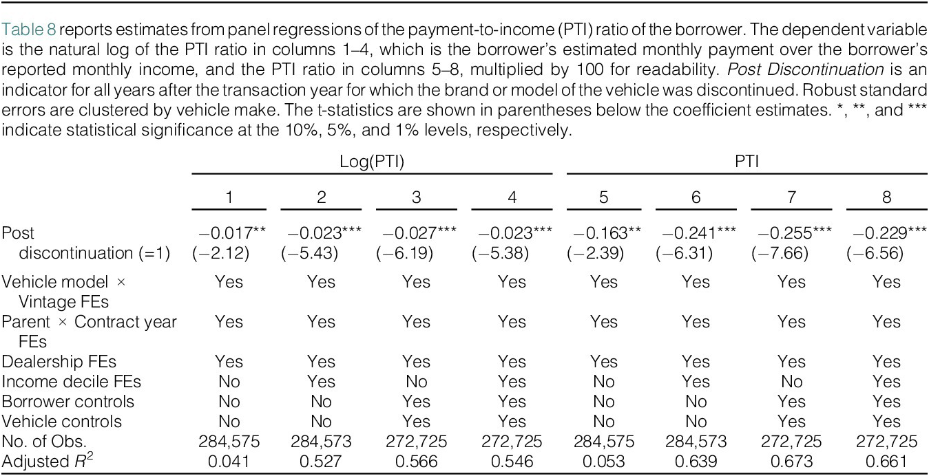
We test this prediction by regressing the log of the borrower’s payment-to-income (PTI) ratio on the post-discontinuation variable and the standard fixed effects. We find a negative and significant effect of discontinuation on the log of PTI (coefficient = −0.017 and $ t $
-stat = −2.12), as displayed in the first column of Table 8. PTI ratios of the purchasers of these vehicles drop by roughly 2% after discontinuation is announced.
$ t $
-stat = −2.12), as displayed in the first column of Table 8. PTI ratios of the purchasers of these vehicles drop by roughly 2% after discontinuation is announced.

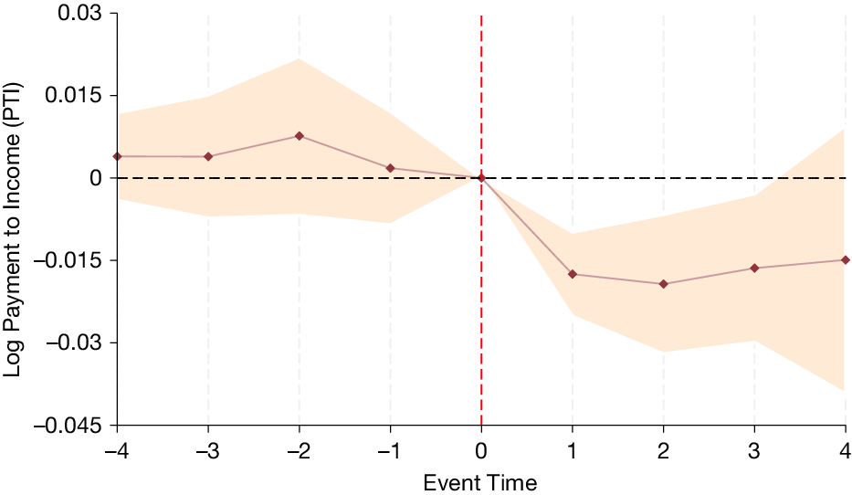
Including fixed effects of the borrower income decile has little impact on the estimated negative coefficient on discontinuation, though it does increase the precision of the estimate, as shown in the second column of Table 8. Introducing borrower and vehicle controls, either with or without fixed effects on borrower income decile, also yields similar estimates, as described in columns 3 and 4 of Table 8. Using the PTI ratio rather than the log as the dependent variable yields similar directional results and significance but lower magnitudes, as displayed in columns 5–8 of Table 8. This is due to a wide distribution in PTI that may skew the results. Figure 4 shows that borrower PTI drops after discontinuation, with no visible pre-trend.
Figure 4 presents differences in the log of the payment-to-income ratio (PTI) across vehicle make-models that were discontinued and those that were not. The plot is the regression coefficients for timing indicators around the year the model was discontinued (discontinuation year = 0). The dependent variable is the log of the borrower’s monthly payment to the borrower’s monthly income. Included fixed effects are Make/Model $ \times $
Vintage Year, Dealership, borrower income decile, and Contract Year
$ \times $
Vintage Year, Dealership, borrower income decile, and Contract Year $ \times $
Parent Company.
$ \times $
Parent Company.

The complete set of empirical findings across down payments, LTVs and PTIs offers consistent support for the argument that income is pledgeable and that lower-income borrowers rely more heavily on IBL, as described in region I of Figure B.1 in the Supplementary Material. Moreover, down payments are generally non-negative in our data, so the Model Implications in Section II suggest that there is a constant component to the dealer markup.Footnote 26 In direct tests, in Table F.5 in the Supplementary Material, we show that dealer dollar margins do not vary with vehicle discontinuation status. These results indicate that dealers indeed earn constant margins across more and less durable assets.
F. Durability and Recovery in Default
In the discussion above, we highlight the role of IBL. For IBL to be important, however, it must be that consumers are able to borrow against their future income and need not rely solely on the physical asset to serve as collateral. In this section, we discuss the direct evidence on post-default lender collections. In particular, is it the case that lenders actually recover from the personal resources of borrowers?
We have data on the recovery proceeds from 76,638 defaulted loans where we observe both income and vehicle recoveries. For this sample, we find that the average proceeds from the sales of repossessed vehicles are $3483. The average cash recovery from the borrower is $1171. We thus find that in default, physical assets and personal borrower resources supply 75% and 25%, respectively, of the total recovery proceeds. These summary statistics show that in the auto loan market, a market in which vehicle collateral is generally deemed to serve a central role, borrower personal income pledges do perform a significant function.
G. IBL to Lower-Income Consumers: Default Recoveries
As outlined in the model developed in Section II, the results in Table 6 showing that a reduction in durability leads to larger down payments demonstrate that IBL is important in the auto financing market. The empirical findings on LTV and PTI in Tables 7 and 8 establish that lower-income borrowers are more heavily relying on IBL than higher-income borrowers.
The default recovery data make possible an additional test of these implications. We show in Table 5 that discontinued vehicles tend to be purchased by lower-income consumers. Given the results in Tables 6–8, the model’s implications are that lower-income borrowers rely relatively more on IBL. We should therefore expect to observe lower vehicle recoveries and higher personal income recoveries from the purchasers of discontinued vehicles who default.
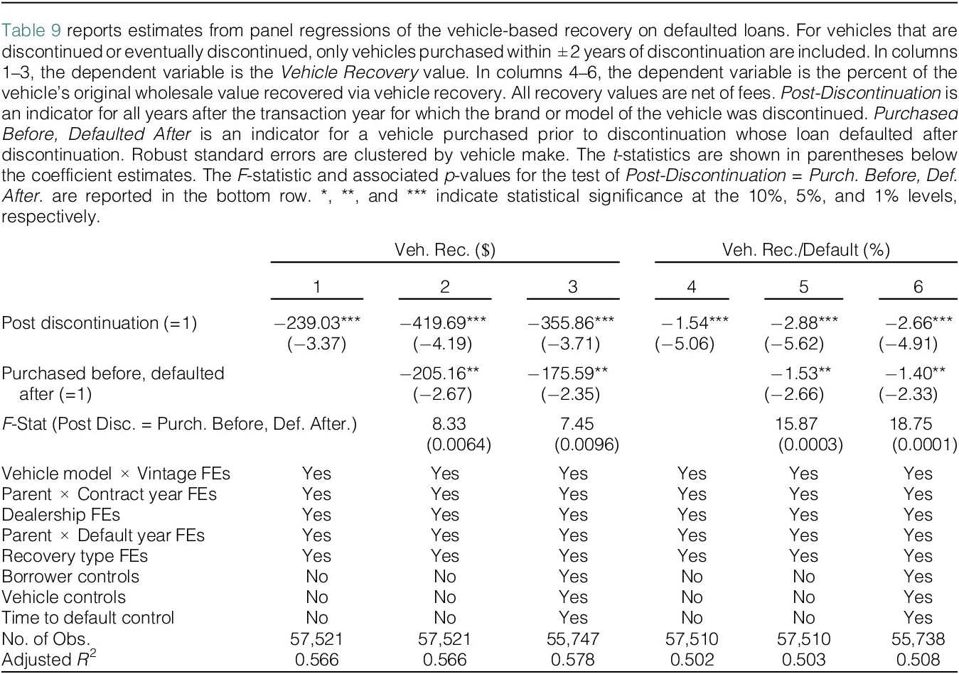
In the extension of the model described in Section II, we discuss the idea that different borrowers may experience varying levels of asset depreciation for the same vehicle. The recovery data enable us to examine this hypothesis, as we can contrast the outcomes for borrowers who purchased vehicles that were later discontinued with outcomes for borrowers who purchased vehicles after the discontinuation announcement. Both types of borrowers experience the impact on their vehicles of a discontinuation, but the borrowers themselves differ in that only the first group of borrowers chose to purchase what were at the time non-discontinued cars. Any observed differences across the two borrower types in their recovery rates would therefore constitute evidence in favor of borrower-dependent depreciation. In order to ensure that the vehicles of these two borrower groups are comparable, for cars that are discontinued or eventually discontinued, only autos purchased within 2 years of a discontinuation are included.
We begin by analyzing recovery rates for borrowers who purchased their vehicles after a discontinuation announcement. Consistent with our labeling in the previous tables, we describe these as Post-Discontinuation transactions. We regress the value of the vehicle recovery on the post-discontinuation indicator, the standard fixed effects and additional fixed effects for the corporate parent × default year, and the form of recovery. We find, as shown in the first column of Table 9, that vehicles purchased post-discontinuation are worth $239.03 less ( $ t $
-stat = −3.37) in repossession. These vehicles are less durable and therefore provide diminished physical recovery proceeds, as expected under the model. It may also be the case that the purchasers of the vehicles are less able to maintain them, resulting in even higher rates of depreciation.
$ t $
-stat = −3.37) in repossession. These vehicles are less durable and therefore provide diminished physical recovery proceeds, as expected under the model. It may also be the case that the purchasers of the vehicles are less able to maintain them, resulting in even higher rates of depreciation.

As a point of contrast, we examine vehicle recovery proceeds from cars purchased prior to discontinuation that experienced default after discontinuation. We label these transactions as Purchase Before, Default After.
Footnote
27 In the second column of Table 9, we show that these vehicles have $205.16 lower ( $ t $
-stat = −2.67) recoveries. The purchasers of these cars did not choose to buy a discontinued auto: discontinuation was an ex post shock that they experienced.Footnote
28 The drop in vehicle recoveries we find for this group therefore constitutes evidence of higher post-discontinuation depreciation that affects the physical asset independent of the borrower type.
$ t $
-stat = −2.67) recoveries. The purchasers of these cars did not choose to buy a discontinued auto: discontinuation was an ex post shock that they experienced.Footnote
28 The drop in vehicle recoveries we find for this group therefore constitutes evidence of higher post-discontinuation depreciation that affects the physical asset independent of the borrower type.
The coefficient on Post Discontinuation in this regression is −419.69 ( $ t $
-stat = −4.19). This coefficient is larger in magnitude than the coefficient on Purchase Before, Default After, with the difference statistically significant at the 5% level. The relatively lower recovery for borrowers who purchased their vehicles after discontinuation, compared to those who experienced discontinuation after purchase, is evidence in favor of borrower-dependent depreciation. This regression includes fixed effects for both model × vintage and parent × default year, so we are comparing outcomes for similar vehicles that defaulted at the same time and that had been discontinued at the time of default. The reduced recovery for post-discontinuation buyers suggests that, perhaps due to financial constraints, these consumers were unable to maintain the values of their vehicles in the same manner as those who purchased them before the discontinuation. Including borrower, vehicle mileage, dealer profit, and time to default controls has little impact on the estimated coefficients on Purchase Before, Default After and Post Discontinuation, as detailed in the third column of Table 9; both remain significant and statistically distinct from each other at the 5% level. Figure F.6 in the Supplementary Material provides a graphical depiction of vehicle recoveries for both borrowers who experienced a discontinuation after purchase and for those who purchased after discontinuation.Footnote
29
$ t $
-stat = −4.19). This coefficient is larger in magnitude than the coefficient on Purchase Before, Default After, with the difference statistically significant at the 5% level. The relatively lower recovery for borrowers who purchased their vehicles after discontinuation, compared to those who experienced discontinuation after purchase, is evidence in favor of borrower-dependent depreciation. This regression includes fixed effects for both model × vintage and parent × default year, so we are comparing outcomes for similar vehicles that defaulted at the same time and that had been discontinued at the time of default. The reduced recovery for post-discontinuation buyers suggests that, perhaps due to financial constraints, these consumers were unable to maintain the values of their vehicles in the same manner as those who purchased them before the discontinuation. Including borrower, vehicle mileage, dealer profit, and time to default controls has little impact on the estimated coefficients on Purchase Before, Default After and Post Discontinuation, as detailed in the third column of Table 9; both remain significant and statistically distinct from each other at the 5% level. Figure F.6 in the Supplementary Material provides a graphical depiction of vehicle recoveries for both borrowers who experienced a discontinuation after purchase and for those who purchased after discontinuation.Footnote
29
A decrease in durability reduces not only the dollar amount recovered from the repossessed asset but also the percentage of the loan balance recovered through liquidation. We find, as detailed in the fourth column of Table 9, that the percentage of the loan balance recovered through liquidation of the vehicle is lower for vehicles purchased after discontinuation. In the fifth column of Table 9, we show that the effect of Post Discontinuation (coefficient = −2.88 and $ t $
-stat = −5.62) is greater in magnitude than the impact of Purchase Before, Default After (coefficient = −1.53 and
$ t $
-stat = −5.62) is greater in magnitude than the impact of Purchase Before, Default After (coefficient = −1.53 and $ t $
-stat = −2.66), and the difference is statistically significant at the 5% level. The results for the specification including the full set of controls outlined in the sixth column of Table 9, are quite similar. These findings buttress the argument that asset depreciation varies by borrower type.
$ t $
-stat = −2.66), and the difference is statistically significant at the 5% level. The results for the specification including the full set of controls outlined in the sixth column of Table 9, are quite similar. These findings buttress the argument that asset depreciation varies by borrower type.
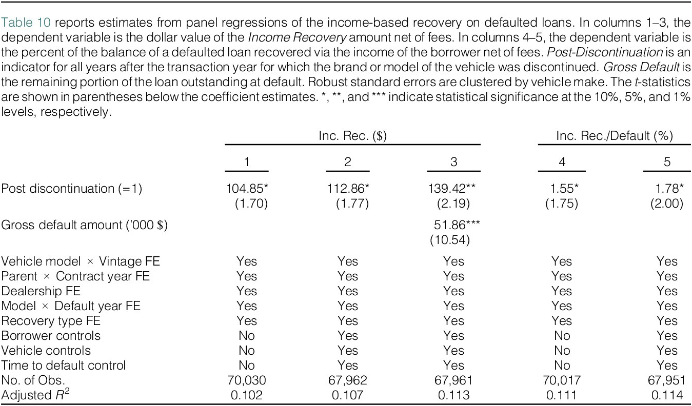
Although it is perhaps unsurprising that vehicle recoveries are lower for discontinued vehicles, it is a novel implication of the model that personal income recoveries as a fraction of the loan balance should be higher for these cars, as they are purchased by lower-income borrowers who rely more heavily on IBL.Footnote
30 We regress the dollar amount of personal post-default payments on the post-discontinuation indicator and the fixed effects described above. We find, as displayed in the first column of Table 10, that the dollar amount weakly increases (coefficient = 104.85 and $ t $
-stat = 1.70) after discontinuation. A similar result holds in the specification with borrower, vehicle, and dealer profit controls, as shown in the second column of Table 10. When including the gross default amount as a control, there is somewhat stronger evidence of an increase in income recovery (coefficient = 139.42 and
$ t $
-stat = 1.70) after discontinuation. A similar result holds in the specification with borrower, vehicle, and dealer profit controls, as shown in the second column of Table 10. When including the gross default amount as a control, there is somewhat stronger evidence of an increase in income recovery (coefficient = 139.42 and $ t $
-stat = 2.19), as displayed in the third column of Table 10.
$ t $
-stat = 2.19), as displayed in the third column of Table 10.

The ratio of personal borrower payments to the defaulted loan balance also weakly increases after discontinuation (coefficient = 1.55 and $ t $
-stat = 1.75), as we detail in the fourth column of Table 10. Including controls somewhat strengthens this conclusion (coefficient = 1.78 and
$ t $
-stat = 1.75), as we detail in the fourth column of Table 10. Including controls somewhat strengthens this conclusion (coefficient = 1.78 and $ t $
-stat = 2.00); the results are displayed in the fifth column of the table.
$ t $
-stat = 2.00); the results are displayed in the fifth column of the table.
Taken together, the results in Tables 9 and 10 support the contention that lower-income borrowers rely more heavily than higher-income borrowers on their income as a collateral source. It is notable that purchasers of discontinued vehicles make larger personal payments after default. These consumers have lower incomes and buy less expensive vehicles. For both of these reasons, one might have expected them to supply smaller personal recoveries relative to their loan balances in the event of a default, yet we find the opposite. The model supplies the intuition for our finding: purchasers of discontinued less durable vehicles must pledge their own income, rather than the quickly depreciating physical asset, in order to receive a loan. In the event of default, a lender therefore must have recourse to their income, as the physical collateral does not have much value.Footnote 31
VI. Conclusion
We study the roles of ABL and IBL in the $1.6 trillion U.S. automotive lending market. We show that tracing the effects of a reduction in the economic durability of assets on financing allows us to assess the overall importance of IBL and its relative usage by higher- and lower-income borrowers. We find that model and make discontinuations generate a negative economic durability shock for used cars: post-discontinuation, holding fixed the model × vintage year, we observe that discontinued vehicles have higher rates of depreciation, lower prices, lower liquidation values, and are purchased by lower-income consumers. After discontinuation, down payments are higher by approximately $79 and LTV ratios increase by 1.4 percentage points. The latter two findings are consistent with a description of the auto market in which IBL plays a meaningful part, lower-income borrowers rely relatively more heavily on it and dealer margins have a constant component.
In a sample of defaulted loans, we find that roughly three-fourths of lender recoveries arise from the vehicle (which serves as the collateral for ABL) and the remaining one-fourth comes from the borrower personally (the source of the guarantee in IBL). For vehicles purchased post-discontinuation, physical collateral recoveries as a percentage of the loan balance are 2.7 percentage points lower, while these recoveries are 1.4 percentage points lower for borrowers who experience discontinuation after purchase. These negative estimates show that discontinuations reduce liquidation values and the gap between the effects is consistent with the claim that depreciation is borrower-dependent. For autos purchased after a discontinuation announcement, the percentage of the loan balance recovered via personal income increases by 1.8 percentage points. The higher personal recoveries on discontinued vehicles may seem surprising given that their purchasers have lower incomes and buy less expensive vehicles. The explanation is that lower-income borrowers make greater use of IBL and must therefore use their personal resources, rather than the collateral value of the vehicle, to cover missing payments in the event of default.
Our theoretical framework draws a sharp contrast between ABL and IBL, but a lender’s ability to secure income-based repayment from a borrower may be linked to its power to repossess a vehicle. This argument suggests that the interaction between a lender’s capabilities to seize income as opposed to collateral is a topic worthy of further analysis.
In the post-financial crisis period, securitization market issuances have increased relatively more for ABL than for IBL forms of financing. This shift may limit relative credit access for lower-income borrowers who rely on IBL. A resulting restriction on the ability of economically disadvantaged consumers to purchase cars may have wide-ranging implications for their welfare. Our results indicate that innovations that aid lenders in monitoring borrower income are likely to be especially helpful for less wealthy consumers who seek auto financing that often offers a gateway to economic opportunity.
Supplementary Material
To view supplementary material for this article, please visit http://doi.org/10.1017/S0022109025102433.


 Open access