

1 Introduction
Pulsars and their winds are among nature’s most powerful particle accelerators, producing particles with energies up to a few PeV. In addition to high-energy radiation from the magnetosphere, the rotational (spin) energy of a neutron star is carried away in the form of a magnetized ultra-relativistic pulsar wind (PW), whose non-thermal emission can be seen from radio to $\unicode[STIX]{x1D6FE}$
-rays, with energies reaching nearly 100 TeV Aharonian et al. (Reference Aharonian, Akhperjanian, Beilicke, Bernlöhr, Börst, Bojahr, Bolz, Coarasa, Contreras and Cortina2004). Recent X-ray and
$\unicode[STIX]{x1D6FE}$
-rays, with energies reaching nearly 100 TeV Aharonian et al. (Reference Aharonian, Akhperjanian, Beilicke, Bernlöhr, Börst, Bojahr, Bolz, Coarasa, Contreras and Cortina2004). Recent X-ray and $\unicode[STIX]{x1D6FE}$
-ray observations suggest that the ratio of energy radiated from the ‘observable’ pulsar wind nebula (PWN) to the energy radiated from the magnetosphere can vary significantly among pulsars. For instance, for the Crab pulsar and its PWN the ratio of the luminosities integrated over the entire electromagnetic spectrumFootnote
1
is
$\unicode[STIX]{x1D6FE}$
-ray observations suggest that the ratio of energy radiated from the ‘observable’ pulsar wind nebula (PWN) to the energy radiated from the magnetosphere can vary significantly among pulsars. For instance, for the Crab pulsar and its PWN the ratio of the luminosities integrated over the entire electromagnetic spectrumFootnote
1
is $L_{\text{PWN}}/L_{\text{PSR}}\simeq 30$
while for the Vela pulsar and its compact PWN it is
$L_{\text{PWN}}/L_{\text{PSR}}\simeq 30$
while for the Vela pulsar and its compact PWN it is $\simeq 0.03$
. The ratio becomes
$\simeq 0.03$
. The ratio becomes ${\sim}1$
if the luminosityFootnote
2
of Vela X (a large structure south of the pulsar bright in radio, X-rays, and high-energy
${\sim}1$
if the luminosityFootnote
2
of Vela X (a large structure south of the pulsar bright in radio, X-rays, and high-energy $\unicode[STIX]{x1D6FE}$
-rays; Grondin et al.
Reference Grondin, Romani, Lemoine-Goumard, Guillemot, Harding and Reposeur2013) is added to the compact PWN luminosity.
$\unicode[STIX]{x1D6FE}$
-rays; Grondin et al.
Reference Grondin, Romani, Lemoine-Goumard, Guillemot, Harding and Reposeur2013) is added to the compact PWN luminosity.
The speed of the PW is highly relativistic immediately beyond the pulsar magnetosphere. However, the interaction with the ambient medium causes the wind to slow down abruptly at a termination shock. Immediately downstream of the termination shock, the flow speed is expected to become mildly relativistic, lower than the speed of sound in ultra-relativistic magnetized plasma but much higher than the sound speed in the ambient medium. It is commonly assumed that the distance to the termination shock from the pulsar, $R_{\text{TS}}\sim ({\dot{E}}/4\unicode[STIX]{x03C0}cP_{\text{amb}})^{1/2}$
, can be estimated by balancing the PW pressureFootnote
3
with the ambient pressure. The flow keeps decelerating further downstream and reaches the contact discontinuity that separates the shocked PW from the surrounding medium shocked in the forward shockFootnote
4
. For a stationary (or slowly moving, subsonic) pulsar, the contact discontinuity sphere (hence the PWN) is expected to be expanding as the pulsar pumps more energy into it, until the radiative and/or adiabatic expansion losses balance the energy input. The shocked PW within the PWN bubble contains ultra-relativistic particles with randomized pitch angles and a magnetic field whose structure also becomes somewhat disordered (see three-dimensional (3-D) simulations of the Crab PWN; Porth et al.
Reference Porth, Vorster, Lyutikov and Engelbrecht2016). Therefore, PWNe are expected to produce synchrotron radiation, responsible for the PWN emission from radio frequencies through X-rays and into the MeV range, and inverse-Compton radiation in the GeV–TeV range (see e.g. the reviews by Kargaltsev & Pavlov Reference Kargaltsev, Pavlov, Bassa, Wang, Cumming and Kaspi2008, Reference Kargaltsev and Pavlov2010; Kargaltsev et al.
Reference Kargaltsev, Cerutti, Lyubarsky and Striani2015; Reynolds et al.
Reference Reynolds, Pavlov, Kargaltsev, Klingler, Renaud and Mereghetti2017).
$R_{\text{TS}}\sim ({\dot{E}}/4\unicode[STIX]{x03C0}cP_{\text{amb}})^{1/2}$
, can be estimated by balancing the PW pressureFootnote
3
with the ambient pressure. The flow keeps decelerating further downstream and reaches the contact discontinuity that separates the shocked PW from the surrounding medium shocked in the forward shockFootnote
4
. For a stationary (or slowly moving, subsonic) pulsar, the contact discontinuity sphere (hence the PWN) is expected to be expanding as the pulsar pumps more energy into it, until the radiative and/or adiabatic expansion losses balance the energy input. The shocked PW within the PWN bubble contains ultra-relativistic particles with randomized pitch angles and a magnetic field whose structure also becomes somewhat disordered (see three-dimensional (3-D) simulations of the Crab PWN; Porth et al.
Reference Porth, Vorster, Lyutikov and Engelbrecht2016). Therefore, PWNe are expected to produce synchrotron radiation, responsible for the PWN emission from radio frequencies through X-rays and into the MeV range, and inverse-Compton radiation in the GeV–TeV range (see e.g. the reviews by Kargaltsev & Pavlov Reference Kargaltsev, Pavlov, Bassa, Wang, Cumming and Kaspi2008, Reference Kargaltsev and Pavlov2010; Kargaltsev et al.
Reference Kargaltsev, Cerutti, Lyubarsky and Striani2015; Reynolds et al.
Reference Reynolds, Pavlov, Kargaltsev, Klingler, Renaud and Mereghetti2017).
In general, studying PWNe provides information about the pulsars that power them, the properties of the surrounding medium, and the physics of the wind-medium interactions. The detailed structure of the interface between the PW and the surrounding ambient medium is not well understood. In an idealized hydrodynamic scenario, the contact discontinuity separates the shocked interstellar medium (ISM) from the shocked PW. Being compressed and heated at the forward shock, the shocked ambient medium emits radiation in spectral lines and continuum. It has been notoriously difficult to identify the forward shock around many young and bright PWNe residing in supernova remnants (SNRs) (including the Crab PWN). However, there is a class of PWNe, associated with supersonically moving pulsars, where both the shocked ambient medium and the shocked PW can be seen. In this review we will focus on observational properties of supersonic pulsar wind nebulae (SPWNe). For a recent theoretical review, see Bykov et al. (Reference Bykov, Amato, Petrov, Krassilchtchikov and Levenfish2017).
1.1 SPWNe – PWNe of supersonic pulsars
In addition to the ISM pressure, the PWN size and morphology can be significantly affected by the ram pressure of the external medium caused by the fast (supersonic) pulsar motion. Indeed, average pulsar 3-D velocities have been found to be $v_{p}\sim 400~\text{km}~\text{s}^{-1}$
for an isotropic velocity distribution (Hobbs et al.
Reference Hobbs, Lorimer, Lyne and Kramer2005). This implies that the majority of pulsars only stay within their host SNR environment for a few tens of kilo-years, although some particularly fast-moving pulsars can leave it even earlier. Once the pulsar leaves its host SNR, it enters a very different environment, with a much lower sound speed,
$v_{p}\sim 400~\text{km}~\text{s}^{-1}$
for an isotropic velocity distribution (Hobbs et al.
Reference Hobbs, Lorimer, Lyne and Kramer2005). This implies that the majority of pulsars only stay within their host SNR environment for a few tens of kilo-years, although some particularly fast-moving pulsars can leave it even earlier. Once the pulsar leaves its host SNR, it enters a very different environment, with a much lower sound speed, $c_{s}\sim 3{-}30~\text{km}~\text{s}^{-1}$
, depending on the ISM phaseFootnote
5
, hence the pulsar motion becomes highly supersonic, i.e.
$c_{s}\sim 3{-}30~\text{km}~\text{s}^{-1}$
, depending on the ISM phaseFootnote
5
, hence the pulsar motion becomes highly supersonic, i.e. $v_{p}/c_{s}\equiv {\mathcal{M}}\gg 1$
, where
$v_{p}/c_{s}\equiv {\mathcal{M}}\gg 1$
, where ${\mathcal{M}}$
is the Mach number.
${\mathcal{M}}$
is the Mach number.
The supersonic motion strongly modifies the PWN appearance and the properties of its emission, making it useful to introduce a separate category of SPWNe. In particular, for an isotropic PW, the forward shock, contact discontinuity, and termination shock shapes resemble paraboloids in the pulsar vicinity but have quite different shapes behind the pulsar (see figure 9 in Gaensler et al. (Reference Gaensler, van der Swaluw, Camilo, Kaspi, Baganoff, Yusef-Zadeh and Manchester2004)). The distance from the pulsar to the apex of the contact discontinuity can be estimated as
 $$\begin{eqnarray}\displaystyle R_{a}\approx \left[\frac{{\dot{E}}f_{\unicode[STIX]{x1D6FA}}}{4\unicode[STIX]{x03C0}c(P_{\text{amb}}+P_{\text{ram}})}\right]^{1/2}. & & \displaystyle\end{eqnarray}$$
At this distance, the PW pressure, $P_{w}={\dot{E}}f_{\unicode[STIX]{x1D6FA}}(4\unicode[STIX]{x03C0}cr^{2})^{-1}$
(
$P_{w}={\dot{E}}f_{\unicode[STIX]{x1D6FA}}(4\unicode[STIX]{x03C0}cr^{2})^{-1}$
( $f_{\unicode[STIX]{x1D6FA}}$
takes into account PW anisotropy), is balanced by the sum of the ambient pressure,
$f_{\unicode[STIX]{x1D6FA}}$
takes into account PW anisotropy), is balanced by the sum of the ambient pressure, $P_{\text{amb}}=\unicode[STIX]{x1D70C}kT(\unicode[STIX]{x1D707}m_{H})^{-1}=1.38\times 10^{-12}n_{H}\unicode[STIX]{x1D707}^{-1}T_{4}~\text{dyn}~\text{cm}^{-2}$
, and the ram pressure,
$P_{\text{amb}}=\unicode[STIX]{x1D70C}kT(\unicode[STIX]{x1D707}m_{H})^{-1}=1.38\times 10^{-12}n_{H}\unicode[STIX]{x1D707}^{-1}T_{4}~\text{dyn}~\text{cm}^{-2}$
, and the ram pressure, $P_{\text{ram}}=\unicode[STIX]{x1D70C}v^{2}=1.67\times 10^{-10}nv_{7}^{2}~\text{dyn}~\text{cm}^{-2}$
(
$P_{\text{ram}}=\unicode[STIX]{x1D70C}v^{2}=1.67\times 10^{-10}nv_{7}^{2}~\text{dyn}~\text{cm}^{-2}$
( $T_{4}=T/10^{4}~\text{K}$
,
$T_{4}=T/10^{4}~\text{K}$
, $v_{7}=v/10^{7}~\text{cm}~\text{s}^{-1}$
,
$v_{7}=v/10^{7}~\text{cm}~\text{s}^{-1}$
, $\unicode[STIX]{x1D707}$
is the mean molecular weight, and
$\unicode[STIX]{x1D707}$
is the mean molecular weight, and $n=\unicode[STIX]{x1D70C}/m_{H}$
is in units of
$n=\unicode[STIX]{x1D70C}/m_{H}$
is in units of $\text{cm}^{-3}$
). Assuming
$\text{cm}^{-3}$
). Assuming $P_{\text{ram}}\gg P_{\text{amb}}$
(or
$P_{\text{ram}}\gg P_{\text{amb}}$
(or ${\mathcal{M}}\gg 1$
), we obtain
${\mathcal{M}}\gg 1$
), we obtain $R_{a}=6.5\times 10^{16}n^{-1/2}f_{\unicode[STIX]{x1D6FA}}^{1/2}{\dot{E}}_{36}^{1/2}v_{7}^{-1}~\text{cm}$
(see e.g. Kargaltsev & Pavlov Reference Kargaltsev and Pavlov2007).
$R_{a}=6.5\times 10^{16}n^{-1/2}f_{\unicode[STIX]{x1D6FA}}^{1/2}{\dot{E}}_{36}^{1/2}v_{7}^{-1}~\text{cm}$
(see e.g. Kargaltsev & Pavlov Reference Kargaltsev and Pavlov2007).
The shocked PW, whose synchrotron emission can be seen in X-rays and radio, is confined between the termination shock and contact discontinuity surfaces. For ${\mathcal{M}}\gg 1$
and a nearly isotropic preshock wind with a small magnetization parameter (see § 2.2), the termination shock acquires a bullet-like shape (Gaensler et al.
Reference Gaensler, van der Swaluw, Camilo, Kaspi, Baganoff, Yusef-Zadeh and Manchester2004; Bucciantini, Amato & Del Zanna Reference Bucciantini, Amato and Del Zanna2005). The length of the bullet and the diameter of the post-termination shock PWN are
${\mathcal{M}}\gg 1$
and a nearly isotropic preshock wind with a small magnetization parameter (see § 2.2), the termination shock acquires a bullet-like shape (Gaensler et al.
Reference Gaensler, van der Swaluw, Camilo, Kaspi, Baganoff, Yusef-Zadeh and Manchester2004; Bucciantini, Amato & Del Zanna Reference Bucciantini, Amato and Del Zanna2005). The length of the bullet and the diameter of the post-termination shock PWN are $\simeq (5{-}6)R_{a}$
and
$\simeq (5{-}6)R_{a}$
and $\simeq 4R_{a}$
, respectively (Bucciantini et al.
Reference Bucciantini, Amato and Del Zanna2005).
$\simeq 4R_{a}$
, respectively (Bucciantini et al.
Reference Bucciantini, Amato and Del Zanna2005).
Parameters of pulsars with SPWNe (from the Australia Telescope National Facility (ATNF) pulsar catalogue; Manchester et al.
Reference Manchester, Hobbs, Teoh and Hobbs2005). The pulsars are listed in order of decreasing ${\dot{E}}$
. Distance
${\dot{E}}$
. Distance $d$
is given in units of kpc, spin-down energy loss rate
$d$
is given in units of kpc, spin-down energy loss rate ${\dot{E}}$
, pulsar characteristic age
${\dot{E}}$
, pulsar characteristic age $\unicode[STIX]{x1D70F}=P/2{\dot{P}}$
, surface magnetic field
$\unicode[STIX]{x1D70F}=P/2{\dot{P}}$
, surface magnetic field $B_{11}$
, and projected pulsar velocity
$B_{11}$
, and projected pulsar velocity $v_{\bot }$
.
$v_{\bot }$
.

Note: Unless specified otherwise the pulsar distances are inferred from the dispersion measure according to Yao, Manchester & Wang (Reference Yao, Manchester and Wang2017) or taken from the individual papers (see references in table 2).
a The supersonic nature of the PWNe powered by these pulsars has not been firmly established.
b Distances are from parallax measurements.
c These are radio-quiet pulsars detected in $\unicode[STIX]{x1D6FE}$
-rays with particularly uncertain distances.
$\unicode[STIX]{x1D6FE}$
-rays with particularly uncertain distances.
d Velocities are based on the estimates from Brownsberger & Romani (Reference Brownsberger and Romani2014).
Additional complexity arises due to the fact that the PW is likely not isotropic but concentrated toward the equatorial plane of the rotating pulsar. Evidence of such anisotropy, at least in young pulsars, is seen in high-resolution Chandra images (e.g. Kargaltsev & Pavlov Reference Kargaltsev, Pavlov, Bassa, Wang, Cumming and Kaspi2008), and it is supported by theoretical modelling (Komissarov & Lyubarsky Reference Komissarov and Lyubarsky2004). Therefore the appearance of an SPWN is expected to depend on the angle between the velocity vector and the spin axis of the pulsar. Vigelius et al. (Reference Vigelius, Melatos, Chatterjee, Gaensler and Ghavamian2007) demonstrated this by performing 3-D hydrodynamical simulations and introducing a latitudinal dependence of the wind power (with the functional form expected for the split vacuum dipole solution). In addition, inhomogeneities in the ambient medium (Vigelius et al.
Reference Vigelius, Melatos, Chatterjee, Gaensler and Ghavamian2007) and ISM entrainment (Morlino, Lyutikov & Vorster Reference Morlino, Lyutikov and Vorster2015) are expected to affect the bow shock shape. Observational confirmation of these expectations comes from X-ray and $H\unicode[STIX]{x1D6FC}$
(and more recently also far-UV, see below) images of SPWNe.
$H\unicode[STIX]{x1D6FC}$
(and more recently also far-UV, see below) images of SPWNe.
2 Current sample of SPWNe
Currently, there are approximately 30 pulsars whose X-ray, radio, or $H\unicode[STIX]{x1D6FC}$
images either clearly show or strongly suggest effects of supersonic motion (see tables 1 and 2). Most of these SPWNe (or SPWN candidates) have been found in X-rays, primarily through high-resolution imaging with Chandra (see figure 2). In eight cases the supersonic PWN morphologies can be seen in radio. In two cases (PSRs B0906–49 and J1437–5959) radio images clearly show SPWNe which are not seen in X-ray images. Finally, there are eight rotation-powered pulsars with detected
$H\unicode[STIX]{x1D6FC}$
images either clearly show or strongly suggest effects of supersonic motion (see tables 1 and 2). Most of these SPWNe (or SPWN candidates) have been found in X-rays, primarily through high-resolution imaging with Chandra (see figure 2). In eight cases the supersonic PWN morphologies can be seen in radio. In two cases (PSRs B0906–49 and J1437–5959) radio images clearly show SPWNe which are not seen in X-ray images. Finally, there are eight rotation-powered pulsars with detected $H\unicode[STIX]{x1D6FC}$
bow shocks, of which seven have X-ray PWN detections (see table 2), with two bow shocks also detected in far-UV. Despite the existence of TeV observations, no SPWN detection in TeV has been reported yet. With the exception of the very young and energetic PSR J0537–6910 in the large Magellanic cloud (LMC) (
$H\unicode[STIX]{x1D6FC}$
bow shocks, of which seven have X-ray PWN detections (see table 2), with two bow shocks also detected in far-UV. Despite the existence of TeV observations, no SPWN detection in TeV has been reported yet. With the exception of the very young and energetic PSR J0537–6910 in the large Magellanic cloud (LMC) ( $\unicode[STIX]{x1D70F}=4.9$
kyr,
$\unicode[STIX]{x1D70F}=4.9$
kyr, ${\dot{E}}=4.9\times 10^{38}~\text{erg}~\text{s}^{-1}$
), which may turn out to be not an SPWN despite the suggestive X-ray PWN morphologyFootnote
6
, the rest of SPWNe are powered by non-recycled pulsars with ages between 10 kyr and 3 Myr, or by much older recycled pulsars; their spin-down powers span the range of
${\dot{E}}=4.9\times 10^{38}~\text{erg}~\text{s}^{-1}$
), which may turn out to be not an SPWN despite the suggestive X-ray PWN morphologyFootnote
6
, the rest of SPWNe are powered by non-recycled pulsars with ages between 10 kyr and 3 Myr, or by much older recycled pulsars; their spin-down powers span the range of $10^{33}{-}10^{37}~\text{erg}~\text{s}^{-1}$
(see figure 1).
$10^{33}{-}10^{37}~\text{erg}~\text{s}^{-1}$
(see figure 1).
Estimated parameters of SPWNe: bow shock apex stand-off distance $r_{\text{BS}}$
, the inclination angle
$r_{\text{BS}}$
, the inclination angle $i$
between the pulsar spin axis and our line of sight, the tail length
$i$
between the pulsar spin axis and our line of sight, the tail length $l$
, the X-ray tail luminosity
$l$
, the X-ray tail luminosity $L_{X}$
(in the 0.5–8 keV band), and the corresponding X-ray efficiency
$L_{X}$
(in the 0.5–8 keV band), and the corresponding X-ray efficiency $\unicode[STIX]{x1D702}_{X}=L_{X}/{\dot{E}}$
. References: [1] – Wang et al. (Reference Wang, Gotthelf, Chu and Dickel2001), [2] – Moon et al. (Reference Moon, Lee, Eikenberry, Koo, Chatterjee, Kaplan, Hester, Cordes, Gallant and Koch-Miramond2004), [3] – Zeiger et al. (Reference Zeiger, Brisken, Chatterjee and Goss2008), [4] – Romani et al. (Reference Romani, Ng, Dodson and Brisken2005), [5] – Gaensler et al. (Reference Gaensler, van der Swaluw, Camilo, Kaspi, Baganoff, Yusef-Zadeh and Manchester2004), [6] – Hales et al. (Reference Hales, Gaensler, Chatterjee, van der Swaluw and Camilo2009), [7] – Yusef-Zadeh & Gaensler (Reference Yusef-Zadeh and Gaensler2005), [8] – Klingler et al. (in prep), [9] – Ng et al. (Reference Ng, Gaensler, Chatterjee and Johnston2010), [10] – Kargaltsev et al. (Reference Kargaltsev, Misanovic, Pavlov, Wong and Garmire2008), [11] – Klingler et al. (Reference Klingler, Kargaltsev, Rangelov, Pavlov, Posselt and Ng2016a
), [12] – Petre, Kuntz & Shelton (Reference Petre, Kuntz and Shelton2002), [13] – Frail et al. (Reference Frail, Giacani, Goss and Dubner1996), [14] – Chatterjee et al. (Reference Chatterjee, Brisken, Vlemmings, Goss, Lazio, Cordes, Thorsett, Fomalont, Lyne and Kramer2009), [15] – Ng et al. (Reference Ng, Romani, Brisken, Chatterjee and Kramer2007), [16] – McGowan et al. (Reference McGowan, Vestrand, Kennea, Zane, Cropper and Córdova2006), [17] – Klingler et al. (Reference Klingler, Rangelov, Kargaltsev, Pavlov, Romani, Posselt, Slane, Temim, Ng and Bucciantini2016b
), [18] – Caraveo et al. (Reference Caraveo, Bignami, De Luca, Mereghetti, Pellizzoni, Mignani, Tur and Becker2003), [19] – Pavlov, Bhattacharyya & Zavlin (Reference Pavlov, Bhattacharyya and Zavlin2010), [20] – Posselt et al. (Reference Posselt, Pavlov, Slane, Romani, Bucciantini, Bykov, Kargaltsev, Weisskopf and Ng2017), [21] – Hui & Becker (Reference Hui and Becker2006), [22] – Becker et al. (Reference Becker, Kramer, Jessner, Taam, Jia, Cheng, Mignani, Pellizzoni, de Luca and Słowikowska2006), [23] – Misanovic, Pavlov & Garmire (Reference Misanovic, Pavlov and Garmire2008), [24] – Hui et al. (Reference Hui, Huang, Trepl, Tetzlaff, Takata, Wu and Cheng2012), [25] – Deller et al. (Reference Deller, Verbiest, Tingay and Bailes2008), [26] – Brownsberger & Romani (Reference Brownsberger and Romani2014), [27] – Camilo et al. (Reference Camilo, Ng, Gaensler, Ransom, Chatterjee, Reynolds and Sarkissian2009), [28] – Marelli et al. (Reference Marelli, Mignani, De Luca, Saz Parkinson, Salvetti, Den Hartog and Wolff2015), [29] – Romani et al. (Reference Romani, Shaw, Camilo, Cotter and Sivakoff2010), [30] – Auchettl et al. (Reference Auchettl, Slane, Romani, Posselt, Pavlov, Kargaltsev, Ng, Temim, Weisskopf and Bykov2015), [31] – De Luca et al. (Reference De Luca, Mignani, Marelli, Salvetti, Sartore, Belfiore, Saz Parkinson, Caraveo and Bignami2013), [32] – De Luca et al. (Reference De Luca, Marelli, Mignani, Caraveo, Hummel, Collins, Shearer, Saz Parkinson, Belfiore and Bignami2011), [33] – Stappers et al. (Reference Stappers, Gaensler, Kaspi, van der Klis and Lewin2003), [34] – Huang et al. (Reference Huang, Kong, Takata, Hui, Lin and Cheng2012), [35] – Kaspi et al. (Reference Kaspi, Gotthelf, Gaensler and Lyutikov2001), [36] – Blazek et al. (Reference Blazek, Gaensler, Chatterjee, van der Swaluw, Camilo and Stappers2006), [37] – Halpern et al. (Reference Halpern, Tomsick, Gotthelf, Camilo, Ng, Bodaghee, Rodriguez, Chaty and Rahoui2014), [38] – Tomsick et al. (Reference Tomsick, Bodaghee, Rodriguez, Chaty, Camilo, Fornasini and Rahoui2012), [39] – Pavan et al. (Reference Pavan, Bordas, Pühlhofer, Filipović, De Horta, O’Brien, Balbo, Walter, Bozzo and Ferrigno2014), [40] – Pavan et al. (Reference Pavan, Pühlhofer, Bordas, Audard, Balbo, Bozzo, Eckert, Ferrigno, Filipović and Verdugo2016), [41] – Gaensler et al. (Reference Gaensler, Chatterjee, Slane, van der Swaluw, Camilo and Hughes2006), [42] – Acciari et al. (Reference Acciari, Aliu, Arlen, Aune, Bautista, Beilicke, Benbow, Bradbury, Buckley and Bugaev2009), [43] – Swartz et al. (Reference Swartz, Pavlov, Clarke, Castelletti, Zavlin, Bucciantini, Karovska, van der Horst, Yukita and Weisskopf2015), [44] – Plucinsky et al. (Reference Plucinsky, Dickel, Slane, Edgar, Gaetz and Smith2002), [45] – Temim et al. (Reference Temim, Slane, Castro, Plucinsky, Gelfand and Dickel2013), [46] – Slane et al. (Reference Slane, Gaensler, van der Swaluw, Hughes and Jenkins2004), [47] – Acero (Reference Acero2011), [48] – Ma et al. (Reference Ma, Ng, Bucciantini, Slane, Gaensler and Temim2016), [49] – Marelli et al. (Reference Marelli, Pizzocaro, De Luca, Gastaldello, Caraveo and Saz Parkinson2016a
), [50] – Gaensler et al. (Reference Gaensler, Stappers, Frail and Johnston1998), [51] – Kramer & Johnston (Reference Kramer and Johnston2008), [52] – Voisin et al. (Reference Voisin, Rowell, Burton, Walsh, Fukui and Aharonian2016), [53] – this work, [54] – Manchester et al. (Reference Manchester, Hobbs, Teoh and Hobbs2005).
$\unicode[STIX]{x1D702}_{X}=L_{X}/{\dot{E}}$
. References: [1] – Wang et al. (Reference Wang, Gotthelf, Chu and Dickel2001), [2] – Moon et al. (Reference Moon, Lee, Eikenberry, Koo, Chatterjee, Kaplan, Hester, Cordes, Gallant and Koch-Miramond2004), [3] – Zeiger et al. (Reference Zeiger, Brisken, Chatterjee and Goss2008), [4] – Romani et al. (Reference Romani, Ng, Dodson and Brisken2005), [5] – Gaensler et al. (Reference Gaensler, van der Swaluw, Camilo, Kaspi, Baganoff, Yusef-Zadeh and Manchester2004), [6] – Hales et al. (Reference Hales, Gaensler, Chatterjee, van der Swaluw and Camilo2009), [7] – Yusef-Zadeh & Gaensler (Reference Yusef-Zadeh and Gaensler2005), [8] – Klingler et al. (in prep), [9] – Ng et al. (Reference Ng, Gaensler, Chatterjee and Johnston2010), [10] – Kargaltsev et al. (Reference Kargaltsev, Misanovic, Pavlov, Wong and Garmire2008), [11] – Klingler et al. (Reference Klingler, Kargaltsev, Rangelov, Pavlov, Posselt and Ng2016a
), [12] – Petre, Kuntz & Shelton (Reference Petre, Kuntz and Shelton2002), [13] – Frail et al. (Reference Frail, Giacani, Goss and Dubner1996), [14] – Chatterjee et al. (Reference Chatterjee, Brisken, Vlemmings, Goss, Lazio, Cordes, Thorsett, Fomalont, Lyne and Kramer2009), [15] – Ng et al. (Reference Ng, Romani, Brisken, Chatterjee and Kramer2007), [16] – McGowan et al. (Reference McGowan, Vestrand, Kennea, Zane, Cropper and Córdova2006), [17] – Klingler et al. (Reference Klingler, Rangelov, Kargaltsev, Pavlov, Romani, Posselt, Slane, Temim, Ng and Bucciantini2016b
), [18] – Caraveo et al. (Reference Caraveo, Bignami, De Luca, Mereghetti, Pellizzoni, Mignani, Tur and Becker2003), [19] – Pavlov, Bhattacharyya & Zavlin (Reference Pavlov, Bhattacharyya and Zavlin2010), [20] – Posselt et al. (Reference Posselt, Pavlov, Slane, Romani, Bucciantini, Bykov, Kargaltsev, Weisskopf and Ng2017), [21] – Hui & Becker (Reference Hui and Becker2006), [22] – Becker et al. (Reference Becker, Kramer, Jessner, Taam, Jia, Cheng, Mignani, Pellizzoni, de Luca and Słowikowska2006), [23] – Misanovic, Pavlov & Garmire (Reference Misanovic, Pavlov and Garmire2008), [24] – Hui et al. (Reference Hui, Huang, Trepl, Tetzlaff, Takata, Wu and Cheng2012), [25] – Deller et al. (Reference Deller, Verbiest, Tingay and Bailes2008), [26] – Brownsberger & Romani (Reference Brownsberger and Romani2014), [27] – Camilo et al. (Reference Camilo, Ng, Gaensler, Ransom, Chatterjee, Reynolds and Sarkissian2009), [28] – Marelli et al. (Reference Marelli, Mignani, De Luca, Saz Parkinson, Salvetti, Den Hartog and Wolff2015), [29] – Romani et al. (Reference Romani, Shaw, Camilo, Cotter and Sivakoff2010), [30] – Auchettl et al. (Reference Auchettl, Slane, Romani, Posselt, Pavlov, Kargaltsev, Ng, Temim, Weisskopf and Bykov2015), [31] – De Luca et al. (Reference De Luca, Mignani, Marelli, Salvetti, Sartore, Belfiore, Saz Parkinson, Caraveo and Bignami2013), [32] – De Luca et al. (Reference De Luca, Marelli, Mignani, Caraveo, Hummel, Collins, Shearer, Saz Parkinson, Belfiore and Bignami2011), [33] – Stappers et al. (Reference Stappers, Gaensler, Kaspi, van der Klis and Lewin2003), [34] – Huang et al. (Reference Huang, Kong, Takata, Hui, Lin and Cheng2012), [35] – Kaspi et al. (Reference Kaspi, Gotthelf, Gaensler and Lyutikov2001), [36] – Blazek et al. (Reference Blazek, Gaensler, Chatterjee, van der Swaluw, Camilo and Stappers2006), [37] – Halpern et al. (Reference Halpern, Tomsick, Gotthelf, Camilo, Ng, Bodaghee, Rodriguez, Chaty and Rahoui2014), [38] – Tomsick et al. (Reference Tomsick, Bodaghee, Rodriguez, Chaty, Camilo, Fornasini and Rahoui2012), [39] – Pavan et al. (Reference Pavan, Bordas, Pühlhofer, Filipović, De Horta, O’Brien, Balbo, Walter, Bozzo and Ferrigno2014), [40] – Pavan et al. (Reference Pavan, Pühlhofer, Bordas, Audard, Balbo, Bozzo, Eckert, Ferrigno, Filipović and Verdugo2016), [41] – Gaensler et al. (Reference Gaensler, Chatterjee, Slane, van der Swaluw, Camilo and Hughes2006), [42] – Acciari et al. (Reference Acciari, Aliu, Arlen, Aune, Bautista, Beilicke, Benbow, Bradbury, Buckley and Bugaev2009), [43] – Swartz et al. (Reference Swartz, Pavlov, Clarke, Castelletti, Zavlin, Bucciantini, Karovska, van der Horst, Yukita and Weisskopf2015), [44] – Plucinsky et al. (Reference Plucinsky, Dickel, Slane, Edgar, Gaetz and Smith2002), [45] – Temim et al. (Reference Temim, Slane, Castro, Plucinsky, Gelfand and Dickel2013), [46] – Slane et al. (Reference Slane, Gaensler, van der Swaluw, Hughes and Jenkins2004), [47] – Acero (Reference Acero2011), [48] – Ma et al. (Reference Ma, Ng, Bucciantini, Slane, Gaensler and Temim2016), [49] – Marelli et al. (Reference Marelli, Pizzocaro, De Luca, Gastaldello, Caraveo and Saz Parkinson2016a
), [50] – Gaensler et al. (Reference Gaensler, Stappers, Frail and Johnston1998), [51] – Kramer & Johnston (Reference Kramer and Johnston2008), [52] – Voisin et al. (Reference Voisin, Rowell, Burton, Walsh, Fukui and Aharonian2016), [53] – this work, [54] – Manchester et al. (Reference Manchester, Hobbs, Teoh and Hobbs2005).

a Radio emission is seen ahead of the pulsar, possibly due to interactions with the SNR shell; no radio tail is seen. The SNR which contains the PWN is seen in $H_{\unicode[STIX]{x1D6FC}}$
, making it challenging to discern whether the
$H_{\unicode[STIX]{x1D6FC}}$
, making it challenging to discern whether the $H_{\unicode[STIX]{x1D6FC}}$
emission is produced by SNR reverse shocks or the PW [2].
$H_{\unicode[STIX]{x1D6FC}}$
emission is produced by SNR reverse shocks or the PW [2].
b The supersonic nature of the PWNe powered by these pulsars has not been firmly established.
3 Magnetic fields and related parameters
PWN magnetic fields can be estimated from the synchrotron luminosity and the spectral slope measured in a chosen emitting region. For a power-law spectrum with a photon index $\unicode[STIX]{x1D6E4}$
, the magnetic field is given by the equationFootnote
7
$\unicode[STIX]{x1D6E4}$
, the magnetic field is given by the equationFootnote
7
 $$\begin{eqnarray}B=\left[\frac{L(\unicode[STIX]{x1D708}_{m},\unicode[STIX]{x1D708}_{M})\unicode[STIX]{x1D70E}_{s}}{{\mathcal{A}}V}\frac{\unicode[STIX]{x1D6E4}-2}{\unicode[STIX]{x1D6E4}-1.5}\frac{\unicode[STIX]{x1D708}_{1}^{1.5-\unicode[STIX]{x1D6E4}}-\unicode[STIX]{x1D708}_{2}^{1.5-\unicode[STIX]{x1D6E4}}}{\unicode[STIX]{x1D708}_{m}^{2-\unicode[STIX]{x1D6E4}}-\unicode[STIX]{x1D708}_{M}^{2-\unicode[STIX]{x1D6E4}}}\right]^{2/7}.\end{eqnarray}$$
Here $L(\unicode[STIX]{x1D708}_{m},\unicode[STIX]{x1D708}_{M})$
is the synchrotron luminosity measured in the frequency range
$L(\unicode[STIX]{x1D708}_{m},\unicode[STIX]{x1D708}_{M})$
is the synchrotron luminosity measured in the frequency range $\unicode[STIX]{x1D708}_{m}<\unicode[STIX]{x1D708}<\unicode[STIX]{x1D708}_{M}$
from a radiating volume
$\unicode[STIX]{x1D708}_{m}<\unicode[STIX]{x1D708}<\unicode[STIX]{x1D708}_{M}$
from a radiating volume $V$
,
$V$
, $\unicode[STIX]{x1D70E}_{s}=w_{B}/w_{e}$
is the ratio of the energy density of magnetic field to that of electrons,
$\unicode[STIX]{x1D70E}_{s}=w_{B}/w_{e}$
is the ratio of the energy density of magnetic field to that of electrons, ${\mathcal{A}}=(e^{2}/3m_{e}c^{2})^{2}(2\unicode[STIX]{x03C0}em_{e}c)^{-1/2}=3.06\times 10^{-14}$
in c.g.s. units, and
${\mathcal{A}}=(e^{2}/3m_{e}c^{2})^{2}(2\unicode[STIX]{x03C0}em_{e}c)^{-1/2}=3.06\times 10^{-14}$
in c.g.s. units, and $\unicode[STIX]{x1D708}_{1}$
and
$\unicode[STIX]{x1D708}_{1}$
and $\unicode[STIX]{x1D708}_{2}$
are the characteristic synchrotron frequencies (
$\unicode[STIX]{x1D708}_{2}$
are the characteristic synchrotron frequencies ( $\unicode[STIX]{x1D708}_{\text{syn}}\simeq eB\unicode[STIX]{x1D6FE}^{2}/2\unicode[STIX]{x03C0}m_{e}c$
) which correspond to the boundary energies (
$\unicode[STIX]{x1D708}_{\text{syn}}\simeq eB\unicode[STIX]{x1D6FE}^{2}/2\unicode[STIX]{x03C0}m_{e}c$
) which correspond to the boundary energies ( $\unicode[STIX]{x1D6FE}_{1}m_{e}c^{2}$
and
$\unicode[STIX]{x1D6FE}_{1}m_{e}c^{2}$
and $\unicode[STIX]{x1D6FE}_{2}m_{e}c^{2}$
) of the electron spectrum (
$\unicode[STIX]{x1D6FE}_{2}m_{e}c^{2}$
) of the electron spectrum ( $dN_{e}/d\unicode[STIX]{x1D6FE}\propto \unicode[STIX]{x1D6FE}^{-p}\propto \unicode[STIX]{x1D6FE}^{-2\unicode[STIX]{x1D6E4}+1}$
;
$dN_{e}/d\unicode[STIX]{x1D6FE}\propto \unicode[STIX]{x1D6FE}^{-p}\propto \unicode[STIX]{x1D6FE}^{-2\unicode[STIX]{x1D6E4}+1}$
; $\unicode[STIX]{x1D6FE}_{1}<\unicode[STIX]{x1D6FE}<\unicode[STIX]{x1D6FE}_{2}$
). The magnetic fields in SPWNe estimated from synchrotron brightness and spectral slope measurements with the aid of (3.1) are in the range of
$\unicode[STIX]{x1D6FE}_{1}<\unicode[STIX]{x1D6FE}<\unicode[STIX]{x1D6FE}_{2}$
). The magnetic fields in SPWNe estimated from synchrotron brightness and spectral slope measurements with the aid of (3.1) are in the range of ${\sim}(5{-}200)\unicode[STIX]{x1D70E}_{s}^{2/7}~\unicode[STIX]{x03BC}\text{G}$
(see Auchettl et al.
Reference Auchettl, Slane, Romani, Posselt, Pavlov, Kargaltsev, Ng, Temim, Weisskopf and Bykov2015; Klingler et al.
Reference Klingler, Kargaltsev, Rangelov, Pavlov, Posselt and Ng2016a
,Reference Klingler, Rangelov, Kargaltsev, Pavlov, Romani, Posselt, Slane, Temim, Ng and Bucciantini
b
; Pavan et al.
Reference Pavan, Pühlhofer, Bordas, Audard, Balbo, Bozzo, Eckert, Ferrigno, Filipović and Verdugo2016). An additional uncertainty in these estimates is caused, in many cases, by unknown values of the boundary frequencies
${\sim}(5{-}200)\unicode[STIX]{x1D70E}_{s}^{2/7}~\unicode[STIX]{x03BC}\text{G}$
(see Auchettl et al.
Reference Auchettl, Slane, Romani, Posselt, Pavlov, Kargaltsev, Ng, Temim, Weisskopf and Bykov2015; Klingler et al.
Reference Klingler, Kargaltsev, Rangelov, Pavlov, Posselt and Ng2016a
,Reference Klingler, Rangelov, Kargaltsev, Pavlov, Romani, Posselt, Slane, Temim, Ng and Bucciantini
b
; Pavan et al.
Reference Pavan, Pühlhofer, Bordas, Audard, Balbo, Bozzo, Eckert, Ferrigno, Filipović and Verdugo2016). An additional uncertainty in these estimates is caused, in many cases, by unknown values of the boundary frequencies $\unicode[STIX]{x1D708}_{1}$
and
$\unicode[STIX]{x1D708}_{1}$
and $\unicode[STIX]{x1D708}_{2}$
, between which the spectrum can be described by a power law. For
$\unicode[STIX]{x1D708}_{2}$
, between which the spectrum can be described by a power law. For $\unicode[STIX]{x1D6E4}>1.5$
(as observed in most of the tails), the estimate of
$\unicode[STIX]{x1D6E4}>1.5$
(as observed in most of the tails), the estimate of $B$
is not sensitive to the
$B$
is not sensitive to the $\unicode[STIX]{x1D708}_{2}$
value as long as
$\unicode[STIX]{x1D708}_{2}$
value as long as $(\unicode[STIX]{x1D708}_{1}/\unicode[STIX]{x1D708}_{2})^{\unicode[STIX]{x1D6E4}-1.5}\ll 1$
. Varying
$(\unicode[STIX]{x1D708}_{1}/\unicode[STIX]{x1D708}_{2})^{\unicode[STIX]{x1D6E4}-1.5}\ll 1$
. Varying $\unicode[STIX]{x1D708}_{1}$
from radio (
$\unicode[STIX]{x1D708}_{1}$
from radio ( ${\sim}$
1 GHz) to X-ray frequencies changes
${\sim}$
1 GHz) to X-ray frequencies changes $B$
by a factor of 2–3, for
$B$
by a factor of 2–3, for $1.5<\unicode[STIX]{x1D6E4}<2$
.
$1.5<\unicode[STIX]{x1D6E4}<2$
. ${\dot{E}}$
(a; in units of
${\dot{E}}$
(a; in units of $\text{erg}~\text{s}^{-1}$
) and age (b; in years) distributions for the pulsars producing the SPWNe from table 1.
$\text{erg}~\text{s}^{-1}$
) and age (b; in years) distributions for the pulsars producing the SPWNe from table 1.

Chandra ACIS images of 18 SPWNe. The panels are numbered in accordance with tables 1 and 2. Chandra images of some of these objects are also shown in Reynolds et al. (Reference Reynolds, Pavlov, Kargaltsev, Klingler, Renaud and Mereghetti2017).

The magnetic field strengths can be used to estimate the Lorentz factors $\unicode[STIX]{x1D6FE}$
, gyration radii
$\unicode[STIX]{x1D6FE}$
, gyration radii $r_{g}$
, and characteristic cooling times
$r_{g}$
, and characteristic cooling times $t_{\text{syn}}$
of electrons radiating photons of energy
$t_{\text{syn}}$
of electrons radiating photons of energy $E$
:
$E$
:
 $$\begin{eqnarray}\displaystyle & \displaystyle \unicode[STIX]{x1D6FE}\sim 10^{8}(E/1~\text{keV})^{1/2}(B/20~\unicode[STIX]{x03BC}\text{G})^{-1/2}, & \displaystyle\end{eqnarray}$$
 $$\begin{eqnarray}\displaystyle & \displaystyle r_{g}\sim 10^{14}(E/1~\text{keV})^{1/2}(B/20~\unicode[STIX]{x03BC}\text{G})^{-3/2}~\text{cm} & \displaystyle\end{eqnarray}$$
 $$\begin{eqnarray}\displaystyle & \displaystyle t_{\text{syn}}\sim 400(E/1~\text{keV})^{-1/2}(B/20~\unicode[STIX]{x03BC}\text{G})^{-3/2}~\text{yr}. & \displaystyle\end{eqnarray}$$
4 SPWN heads: connection to viewing angle and pulsar magnetosphere geometry
As the initially strongly magnetized wind flows away from the pulsar’s magnetosphere, its magnetic energy is likely to be at least partly converted into the particle energy. According to the currently-popular models, this occurs due to magnetic field reconnection in a region around the equatorial plane. If the pulsar is an oblique rotator (i.e. its magnetic dipole axis is inclined to the spin axis), one expects ‘corrugated’ current sheets to be formed, with regions of oppositely directed magnetic fields susceptible to reconnection (see e.g. Lyubarsky & Kirk Reference Lyubarsky and Kirk2001 for details). Since the size of the reconnection region is expected to be larger for larger obliquity angles $\unicode[STIX]{x1D6FC}$
, the magnetic-to-kinetic energy conversion may be more efficient for pulsars with larger
$\unicode[STIX]{x1D6FC}$
, the magnetic-to-kinetic energy conversion may be more efficient for pulsars with larger $\unicode[STIX]{x1D6FC}$
. Such pulsars may exhibit brighter PWNe, with more pronounced equatorial components (e.g. the Crab PWN). It is less clear what happens at small
$\unicode[STIX]{x1D6FC}$
. Such pulsars may exhibit brighter PWNe, with more pronounced equatorial components (e.g. the Crab PWN). It is less clear what happens at small $\unicode[STIX]{x1D6FC}$
; likely, the magnetic-to-kinetic energy conversion would still take place, but outflows along the spin axis (‘jets’) would be more pronounced than the equatorial ‘tori’Footnote
8
(Bühler & Giomi Reference Bühler and Giomi2016). Examples of such morphologies for young, subsonic pulsars are the G11.2–0.3, Kes 75 and MSH 15–52 PWNe, which exhibit relatively less luminous tori in the X-ray images (see figure 3). For SPWNe, the identification of the equatorial and polar components is more challenging.
$\unicode[STIX]{x1D6FC}$
; likely, the magnetic-to-kinetic energy conversion would still take place, but outflows along the spin axis (‘jets’) would be more pronounced than the equatorial ‘tori’Footnote
8
(Bühler & Giomi Reference Bühler and Giomi2016). Examples of such morphologies for young, subsonic pulsars are the G11.2–0.3, Kes 75 and MSH 15–52 PWNe, which exhibit relatively less luminous tori in the X-ray images (see figure 3). For SPWNe, the identification of the equatorial and polar components is more challenging.
Chandra ACIS images of PWNe where axial outflows (along the pulsar spin axis) dominate equatorial components (tori).

In the X-ray images shown in figure 2 one can often (but not always; see examples below) identify relatively bright and compact PWN ‘heads’ accompanied by much dimmer (in terms of surface brightness) extended tails. Recent deep, high-resolution Chandra observations revealed fine structures of several bright heads with contrasting morphologies (cf. the insets in panels 10 and 16 in figure 2). For instance, the head of the B0355 $+$
54 PWN looks like a symmetric, filled ‘dome’, brighter near the axis than on the sides (Klingler et al.
Reference Klingler, Rangelov, Kargaltsev, Pavlov, Romani, Posselt, Slane, Temim, Ng and Bucciantini2016b
). In contrast, the head of the J1509–5058 PWN, looks like two bent tails (Klingler et al.
Reference Klingler, Kargaltsev, Rangelov, Pavlov, Posselt and Ng2016a
), with almost no emission between them, except for a short southwest extension just behind the pulsarFootnote
9
. This structure is remarkably similar to the Geminga PWN (Posselt et al.
Reference Posselt, Pavlov, Slane, Romani, Bucciantini, Bykov, Kargaltsev, Weisskopf and Ng2017; see panel 17 in figure 2), just the angular size of the latter is larger, in accordance with the smaller distance (250 pc versus 4 kpc). The bow-shaped X-ray emission can be associated with either a limb-brightened shell formed by the shocked PW downstream of the termination shock or pulsar jets bent by the ram pressure of the oncoming ISM. In the former case, a lack of diffuse emission in between the lateral tails would require a non-uniform magnetic field in the emitting shell, possibly caused by amplification of the ISM magnetic field component perpendicular to the pulsar’s velocity vector (Posselt et al.
Reference Posselt, Pavlov, Slane, Romani, Bucciantini, Bykov, Kargaltsev, Weisskopf and Ng2017). In the latter scenario, the winds of J1509–5058 and Geminga must be dominated by luminous polar components (as in the PWNe shown in figure 3) rather than by the equatorial component (as in the Crab and Vela PWNe). If the lateral tails of the J1509–5850 head are indeed bent jets, it may be difficult to explain the ordered helical magnetic field morphology in the extended tail (as suggested by radio polarimetry; Ng et al.
Reference Ng, Gaensler, Chatterjee and Johnston2010); such a structure would be more natural for the axially symmetric case (Romanova, Chulsky & Lovelace Reference Romanova, Chulsky and Lovelace2005), when the pulsar spin axis (hence the jet directions) is co-aligned with the velocity vector.
$+$
54 PWN looks like a symmetric, filled ‘dome’, brighter near the axis than on the sides (Klingler et al.
Reference Klingler, Rangelov, Kargaltsev, Pavlov, Romani, Posselt, Slane, Temim, Ng and Bucciantini2016b
). In contrast, the head of the J1509–5058 PWN, looks like two bent tails (Klingler et al.
Reference Klingler, Kargaltsev, Rangelov, Pavlov, Posselt and Ng2016a
), with almost no emission between them, except for a short southwest extension just behind the pulsarFootnote
9
. This structure is remarkably similar to the Geminga PWN (Posselt et al.
Reference Posselt, Pavlov, Slane, Romani, Bucciantini, Bykov, Kargaltsev, Weisskopf and Ng2017; see panel 17 in figure 2), just the angular size of the latter is larger, in accordance with the smaller distance (250 pc versus 4 kpc). The bow-shaped X-ray emission can be associated with either a limb-brightened shell formed by the shocked PW downstream of the termination shock or pulsar jets bent by the ram pressure of the oncoming ISM. In the former case, a lack of diffuse emission in between the lateral tails would require a non-uniform magnetic field in the emitting shell, possibly caused by amplification of the ISM magnetic field component perpendicular to the pulsar’s velocity vector (Posselt et al.
Reference Posselt, Pavlov, Slane, Romani, Bucciantini, Bykov, Kargaltsev, Weisskopf and Ng2017). In the latter scenario, the winds of J1509–5058 and Geminga must be dominated by luminous polar components (as in the PWNe shown in figure 3) rather than by the equatorial component (as in the Crab and Vela PWNe). If the lateral tails of the J1509–5850 head are indeed bent jets, it may be difficult to explain the ordered helical magnetic field morphology in the extended tail (as suggested by radio polarimetry; Ng et al.
Reference Ng, Gaensler, Chatterjee and Johnston2010); such a structure would be more natural for the axially symmetric case (Romanova, Chulsky & Lovelace Reference Romanova, Chulsky and Lovelace2005), when the pulsar spin axis (hence the jet directions) is co-aligned with the velocity vector.
The quite different ‘filled’ morphology of the B0355 $+$
53 PWN head could be due to different mutual orientations of the pulsar’s spin axis, magnetic dipole axis, velocity vector and the line of sight. Some information on these orientations could be inferred from the pulsar’s signatures at different energies. For instance, Geminga is a
$+$
53 PWN head could be due to different mutual orientations of the pulsar’s spin axis, magnetic dipole axis, velocity vector and the line of sight. Some information on these orientations could be inferred from the pulsar’s signatures at different energies. For instance, Geminga is a $\unicode[STIX]{x1D6FE}$
-ray pulsar (as well as PSR B1509–58) with no bright radio emission, while PSR B0355
$\unicode[STIX]{x1D6FE}$
-ray pulsar (as well as PSR B1509–58) with no bright radio emission, while PSR B0355 $+$
64 was not detected in
$+$
64 was not detected in $\unicode[STIX]{x1D6FE}$
-rays but is quite bright in radio. One can speculate that Geminga and J1509–5850 are moving in the plane of the sky, and their spin axes are nearly perpendicular to the velocity vectors and to the line of sight (this assumption would be consistent with the jet interpretation of the lateral tails). On the contrary, the spin axis of B0355
$\unicode[STIX]{x1D6FE}$
-rays but is quite bright in radio. One can speculate that Geminga and J1509–5850 are moving in the plane of the sky, and their spin axes are nearly perpendicular to the velocity vectors and to the line of sight (this assumption would be consistent with the jet interpretation of the lateral tails). On the contrary, the spin axis of B0355 $+$
54 could be nearly aligned with the line of sight, in which case the ‘dome’ would be interpreted as the equatorial torus distorted by the ram pressure while the central brightening would be the sky projection of the bent jets. Thus, it is quite plausible that the qualitative morphological differences in the appearances of PWN heads can be attributed to geometrical factors (i.e. the angles between the line of sight, velocity vector, spin axis and magnetic dipole axis).
$+$
54 could be nearly aligned with the line of sight, in which case the ‘dome’ would be interpreted as the equatorial torus distorted by the ram pressure while the central brightening would be the sky projection of the bent jets. Thus, it is quite plausible that the qualitative morphological differences in the appearances of PWN heads can be attributed to geometrical factors (i.e. the angles between the line of sight, velocity vector, spin axis and magnetic dipole axis).
Since the pulsar light curves in different energy ranges should also depend on the same geometrical factors, it is interesting to look for correlations between the PWN head shapes and light curves. For instance, both the $\unicode[STIX]{x1D6FE}$
-ray and radio light curves of PSRs J1509–5850 and B1706–44 are remarkably similar, not only in shapes but also in phase shifts between the
$\unicode[STIX]{x1D6FE}$
-ray and radio light curves of PSRs J1509–5850 and B1706–44 are remarkably similar, not only in shapes but also in phase shifts between the $\unicode[STIX]{x1D6FE}$
-ray and radio pulses (see figure 4), which implies similar geometries and allows one to expect similar PWN morphologies. We see in figure 4 that the B1706–44 X-ray PWN shows clear jets (without obvious bending in the pulsar vicinity) and a relatively underluminous equatorial component (in contrast to the Crab). Although faint, the large-scale morphology of the B1706–44 PWN suggests that the pulsar is moving at the position angle (east of north) of approximately
$\unicode[STIX]{x1D6FE}$
-ray and radio pulses (see figure 4), which implies similar geometries and allows one to expect similar PWN morphologies. We see in figure 4 that the B1706–44 X-ray PWN shows clear jets (without obvious bending in the pulsar vicinity) and a relatively underluminous equatorial component (in contrast to the Crab). Although faint, the large-scale morphology of the B1706–44 PWN suggests that the pulsar is moving at the position angle (east of north) of approximately $80^{\circ }$
(Ng & Romani Reference Ng and Romani2008). Thus, although the PWN head morphologies do not look exactly the same, one could imagine that if B1706–44 were moving faster and had even more pronounced jets, its PWN in the pulsar vicinity could look like the one around J1509–5850. The radio and
$80^{\circ }$
(Ng & Romani Reference Ng and Romani2008). Thus, although the PWN head morphologies do not look exactly the same, one could imagine that if B1706–44 were moving faster and had even more pronounced jets, its PWN in the pulsar vicinity could look like the one around J1509–5850. The radio and $\unicode[STIX]{x1D6FE}$
-ray light curves of the Mouse pulsar (J1747–2958) are similar to those of PSRs J1509–5058 and J1709–4429 (see figure 4). The only difference is that the
$\unicode[STIX]{x1D6FE}$
-ray light curves of the Mouse pulsar (J1747–2958) are similar to those of PSRs J1509–5058 and J1709–4429 (see figure 4). The only difference is that the $\unicode[STIX]{x1D6FE}$
-ray pulse of PSR J1747–2958 is slightly wider (with a deeper trough) and more asymmetric compared to those of PSRs J1509–5058 and J1709–4429. All three pulsars display single radio peaks with very similar phase separation from the
$\unicode[STIX]{x1D6FE}$
-ray pulse of PSR J1747–2958 is slightly wider (with a deeper trough) and more asymmetric compared to those of PSRs J1509–5058 and J1709–4429. All three pulsars display single radio peaks with very similar phase separation from the $\unicode[STIX]{x1D6FE}$
pulses. According to the outer gap magnetospheric emission models, this implies a fairly large magnetic inclination angle (so that both
$\unicode[STIX]{x1D6FE}$
pulses. According to the outer gap magnetospheric emission models, this implies a fairly large magnetic inclination angle (so that both $\unicode[STIX]{x1D6FE}$
-ray and radio pulsations can be seen). It is likely that these angles are somewhat larger for PSR J1747–2958 than those of PSRs J1509–5058 and J1709–4429. These considerations help to interpret the appearances of the compact nebulae by suggesting that the equatorial outflow dominates over the polar outflow components in these cases.
$\unicode[STIX]{x1D6FE}$
-ray and radio pulsations can be seen). It is likely that these angles are somewhat larger for PSR J1747–2958 than those of PSRs J1509–5058 and J1709–4429. These considerations help to interpret the appearances of the compact nebulae by suggesting that the equatorial outflow dominates over the polar outflow components in these cases.
Comparison of the PWN morphologies and pulsar light curves for PSRs J1509–5850, B1706–44, and J1747–2858 (top to bottom). The very similar light curves of all three pulsars (both in radio and $\unicode[STIX]{x1D6FE}$
-rays) suggest similar angles between the spin axis and the line of sight,
$\unicode[STIX]{x1D6FE}$
-rays) suggest similar angles between the spin axis and the line of sight, $\unicode[STIX]{x1D701}$
, and between the spin and magnetic axes,
$\unicode[STIX]{x1D701}$
, and between the spin and magnetic axes, $\unicode[STIX]{x1D6FC}$
. The contour drawn on top of the Mouse PWN image represents a possible extent of the equatorial outflow affected by the ram pressure (the outflow is in the plane of the shown contour which is symmetric with respect the pulsar velocity direction but appears to be asymmetric once projected onto the sky; Klingler et al. in prep.).
$\unicode[STIX]{x1D6FC}$
. The contour drawn on top of the Mouse PWN image represents a possible extent of the equatorial outflow affected by the ram pressure (the outflow is in the plane of the shown contour which is symmetric with respect the pulsar velocity direction but appears to be asymmetric once projected onto the sky; Klingler et al. in prep.).

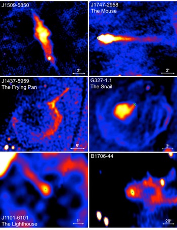
Extended tails behind four pulsars. The X-ray images are obtained with Chandra ACIS. For the Mouse PWN and the J1509–5850 PWN, combined X-ray (red) and radio (blue) images are shown.

Interestingly, we do not see bright heads in the X-ray PWNe of some supersonic pulsars, even those with relatively bright X-ray tails (e.g. PSR J1101–6101 and J0357 $+$
3205; panels 9 and 21 in figure 2). In some of those cases, however, the heads may be too compact to resolve because of high pulsar velocities and large distances.
$+$
3205; panels 9 and 21 in figure 2). In some of those cases, however, the heads may be too compact to resolve because of high pulsar velocities and large distances.
SPWNe can also display contrasting radio morphologies. X-ray bright PWN heads may or may not be bright in radio. For instance the Mouse PWN has the head which is bright in both X-rays and radio, while there is very little (if any) radio emission from the head of the J1509–5058 PWN, although it is bright in X-rays (see figure 5).
Understanding the causes for the differing head (and, possibly, tail; see § 5) morphologies in SPWNe is important because it can help to determine the orientation of the pulsar spin axis with respect to the line of sight and to the pulsar velocity vector (see figure 6). The former is the angle $\unicode[STIX]{x1D701}$
, an important parameter for comparing magnetospheric emission models with the
$\unicode[STIX]{x1D701}$
, an important parameter for comparing magnetospheric emission models with the $\unicode[STIX]{x1D6FE}$
-ray and radio light curves (see e.g. Pierbattista et al.
Reference Pierbattista, Harding, Gonthier and Grenier2016). The angle between the spin axis and the pulsar velocity (the direction of the ‘natal’ kick for not too old pulsars) has important implications for the supernova explosion models (Ng & Romani Reference Ng and Romani2007). SPWNe are particularly suitable for this purpose because the projected neutron star velocity can be inferred from the PWN morphology in the absence of neutron star proper motion measurement.
$\unicode[STIX]{x1D6FE}$
-ray and radio light curves (see e.g. Pierbattista et al.
Reference Pierbattista, Harding, Gonthier and Grenier2016). The angle between the spin axis and the pulsar velocity (the direction of the ‘natal’ kick for not too old pulsars) has important implications for the supernova explosion models (Ng & Romani Reference Ng and Romani2007). SPWNe are particularly suitable for this purpose because the projected neutron star velocity can be inferred from the PWN morphology in the absence of neutron star proper motion measurement.
Chandra images of SPWNe that likely move with mildly supersonic velocities. A schematic diagram of a possible geometry is shown for each object, with the jets bent by the ram pressure. The green arrows indicate the inferred direction the velocity vector.

5 Pulsar tails
As supersonic pulsars move through the ISM, the ram pressure confines and channels the PW in the direction opposite to the pulsar’s relative velocity with respect to the local ISM. Therefore, on large spatial scales (compared to the termination shock bullet size) one expects to see a pulsar tail – an extended, ram-pressure-confined structure behind the pulsar (see figures 5 and 7). Several pulsar tails have now been discerned above the background for up to a few parsecs from their parent pulsars. The longest known tails are those of PSR J1509–5850, whose projected visible length spans 7 pc (at $d=3.8$
kpc) in X-rays and
$d=3.8$
kpc) in X-rays and ${\sim}10$
pc in radio (Ng et al.
Reference Ng, Gaensler, Chatterjee and Johnston2010; Klingler et al.
Reference Klingler, Kargaltsev, Rangelov, Pavlov, Posselt and Ng2016a
), and the Mouse PWN, whose X-ray and radio tails span 1 and 17 pc, respectively (at
${\sim}10$
pc in radio (Ng et al.
Reference Ng, Gaensler, Chatterjee and Johnston2010; Klingler et al.
Reference Klingler, Kargaltsev, Rangelov, Pavlov, Posselt and Ng2016a
), and the Mouse PWN, whose X-ray and radio tails span 1 and 17 pc, respectively (at $d=5$
kpc; Gaensler et al.
Reference Gaensler, van der Swaluw, Camilo, Kaspi, Baganoff, Yusef-Zadeh and Manchester2004).
$d=5$
kpc; Gaensler et al.
Reference Gaensler, van der Swaluw, Camilo, Kaspi, Baganoff, Yusef-Zadeh and Manchester2004).
Radio images of pulsar tails: J1509–5850 (ATCA, 5 GHz), J1747–2958 (VLA, 1.5 GHz), J1437–5959 (MOST, 843 MHz), G327–1.1 (MOST, 843 MHz), J1101–6101 (MOST, 843 MHz), and B1706–44 (VLA, 1.4 GHz). The green crosses mark the positions of the pulsars (for the Snail no pulsations are detected and the cross shows the position of the X-ray point source).
On large scales, the shapes of many pulsar tails (e.g. B1929 $+$
10 – Wang, Li & Begelman Reference Wang, Li and Begelman1993, Becker et al.
Reference Becker, Kramer, Jessner, Taam, Jia, Cheng, Mignani, Pellizzoni, de Luca and Słowikowska2006, Misanovic et al.
Reference Misanovic, Pavlov and Garmire2008; J1509–5850 – Klingler et al.
Reference Klingler, Kargaltsev, Rangelov, Pavlov, Posselt and Ng2016a
; J1437–5959 – Ng et al.
Reference Ng, Bucciantini, Gaensler, Camilo, Chatterjee and Bouchard2012) can be crudely approximated by cones that widen with distance from the pulsar as the outflow slows down and expands (see figure 2). However, in some cases the tail brightness can be strongly non-uniform showing more complex structures that can be described as expanding ‘bubbles’ (e.g. the SPWNe of PSR J1741–2054; see panel 19 in figure 2; also Auchettl et al.
Reference Auchettl, Slane, Romani, Posselt, Pavlov, Kargaltsev, Ng, Temim, Weisskopf and Bykov2015. The bubbles and the rapid widening of tails can be attributed to non-uniformities in the ISM, instabilities in the backflow from the pulsar bow shock (van Kerkwijk & Ingle Reference van Kerkwijk and Ingle2008), or entrainment (mass loading of the ISM into the PW; Morlino et al.
Reference Morlino, Lyutikov and Vorster2015). Some tails, such as those of PSRs J1741–2054 (Auchettl et al.
Reference Auchettl, Slane, Romani, Posselt, Pavlov, Kargaltsev, Ng, Temim, Weisskopf and Bykov2015) and B0355
$+$
10 – Wang, Li & Begelman Reference Wang, Li and Begelman1993, Becker et al.
Reference Becker, Kramer, Jessner, Taam, Jia, Cheng, Mignani, Pellizzoni, de Luca and Słowikowska2006, Misanovic et al.
Reference Misanovic, Pavlov and Garmire2008; J1509–5850 – Klingler et al.
Reference Klingler, Kargaltsev, Rangelov, Pavlov, Posselt and Ng2016a
; J1437–5959 – Ng et al.
Reference Ng, Bucciantini, Gaensler, Camilo, Chatterjee and Bouchard2012) can be crudely approximated by cones that widen with distance from the pulsar as the outflow slows down and expands (see figure 2). However, in some cases the tail brightness can be strongly non-uniform showing more complex structures that can be described as expanding ‘bubbles’ (e.g. the SPWNe of PSR J1741–2054; see panel 19 in figure 2; also Auchettl et al.
Reference Auchettl, Slane, Romani, Posselt, Pavlov, Kargaltsev, Ng, Temim, Weisskopf and Bykov2015. The bubbles and the rapid widening of tails can be attributed to non-uniformities in the ISM, instabilities in the backflow from the pulsar bow shock (van Kerkwijk & Ingle Reference van Kerkwijk and Ingle2008), or entrainment (mass loading of the ISM into the PW; Morlino et al.
Reference Morlino, Lyutikov and Vorster2015). Some tails, such as those of PSRs J1741–2054 (Auchettl et al.
Reference Auchettl, Slane, Romani, Posselt, Pavlov, Kargaltsev, Ng, Temim, Weisskopf and Bykov2015) and B0355 $+$
54 (Klingler et al.
Reference Klingler, Rangelov, Kargaltsev, Pavlov, Romani, Posselt, Slane, Temim, Ng and Bucciantini2016b
), exhibit noticeable ‘bendings’ at large distances from the pulsars, which could be attributed to ISM winds. Although Chandra, with its superior angular resolution and low background, delivers better images than XMM-Newton for most pulsar tails, some tails have been studied with XMM-Newton as well (e.g. B1929
$+$
54 (Klingler et al.
Reference Klingler, Rangelov, Kargaltsev, Pavlov, Romani, Posselt, Slane, Temim, Ng and Bucciantini2016b
), exhibit noticeable ‘bendings’ at large distances from the pulsars, which could be attributed to ISM winds. Although Chandra, with its superior angular resolution and low background, delivers better images than XMM-Newton for most pulsar tails, some tails have been studied with XMM-Newton as well (e.g. B1929 $+$
10 – Becker et al.
Reference Becker, Kramer, Jessner, Taam, Jia, Cheng, Mignani, Pellizzoni, de Luca and Słowikowska2006; J2055
$+$
10 – Becker et al.
Reference Becker, Kramer, Jessner, Taam, Jia, Cheng, Mignani, Pellizzoni, de Luca and Słowikowska2006; J2055 $+$
2539 – Marelli et al.
Reference Marelli, Pizzocaro, De Luca, Gastaldello, Caraveo and Saz Parkinson2016a
).
$+$
2539 – Marelli et al.
Reference Marelli, Pizzocaro, De Luca, Gastaldello, Caraveo and Saz Parkinson2016a
).
Radio polarimetry of two extended tails (the Mouse and J1509–5058; Yusef-Zadeh & Gaensler Reference Yusef-Zadeh and Gaensler2005 and Ng et al. Reference Ng, Gaensler, Chatterjee and Johnston2010) shows that the magnetic field direction is predominantly transverse in the J1509–5058 tail while it is aligned with the tail in the case of the Mouse. This could indicate that the spin axis is more aligned with the velocity vector in J1509–5058 than in J1747–2858 (see figure 3 in Romanova et al. Reference Romanova, Chulsky and Lovelace2005). This, however, would be at odds with the jet interpretation of the lateral outflows in the J1509–5058 PWN head.
Furthermore, the brightness of the radio tail in the Mouse decreases with distance from the pulsar, whereas in the J1509–5850 and J1101–6101 tails the radio brightness increases with the distance from the pulsar and peaks around 4 pc and 1.7 pc (at $d=3.8$
kpc for J1509–5850 and
$d=3.8$
kpc for J1509–5850 and $d=7$
kpc for J1101–6101). Such radio surface brightness behaviour could be explained if the PWN magnetic field becomes stronger further down the tail. It is possible for a helical magnetic field configuration if the flow velocity,
$d=7$
kpc for J1101–6101). Such radio surface brightness behaviour could be explained if the PWN magnetic field becomes stronger further down the tail. It is possible for a helical magnetic field configuration if the flow velocity, $v_{\text{tail}}$
, decreases rapidly enough with distance from the pulsar, which may lead to an increase in the magnetic field strength (
$v_{\text{tail}}$
, decreases rapidly enough with distance from the pulsar, which may lead to an increase in the magnetic field strength ( $B_{\text{tail}}\propto v_{\text{tail}}^{-1}S_{\text{tail}}^{-1/2}$
, where
$B_{\text{tail}}\propto v_{\text{tail}}^{-1}S_{\text{tail}}^{-1/2}$
, where $S_{\text{tail}}$
is the cross-sectional area of the tail; see e.g. Bucciantini et al.
Reference Bucciantini, Amato and Del Zanna2005). The G327.1–1.1 (Snail) PWNe contains an undetected pulsar whose tail radio brightness remains constant over its
$S_{\text{tail}}$
is the cross-sectional area of the tail; see e.g. Bucciantini et al.
Reference Bucciantini, Amato and Del Zanna2005). The G327.1–1.1 (Snail) PWNe contains an undetected pulsar whose tail radio brightness remains constant over its ![]() length until it connects to a spherical structure (most likely a reverse shock, as the PWN is located inside its SNR; see figure 7; Ma et al.
Reference Ma, Ng, Bucciantini, Slane, Gaensler and Temim2016).
length until it connects to a spherical structure (most likely a reverse shock, as the PWN is located inside its SNR; see figure 7; Ma et al.
Reference Ma, Ng, Bucciantini, Slane, Gaensler and Temim2016).
The PWN of PSR J1437–5959 (the Frying Pan; figure 7) is not seen in X-rays, although it is prominent in radio and displays a long radio tail which fades with distance from the pulsar until it becomes brighter near the shell of the alleged SNR G315.9–0.0 (see Ng et al. Reference Ng, Bucciantini, Gaensler, Camilo, Chatterjee and Bouchard2012). Another possible example of such a PWN is the one of PSR B0906–49 (J0908–4913) which has been discovered in radio (Gaensler et al. Reference Gaensler, Stappers, Frail and Johnston1998) but was not detected in the subsequent Chandra ACIS observation (Kargaltsev et al. Reference Kargaltsev, Durant, Pavlov and Garmire2012). It is currently unclear what makes these PWNe so underluminous in X-rays. A natural explanation could be a lack of sufficiently energetic particles which might be due to a magnetosphere geometry unfavourable for accelerating particles to high energies. However, for PSR B0906–49, radio timing observations suggest that it is an orthogonal rotator with the pulsar’s spin axis and direction of motion aligned (Kramer & Johnston Reference Kramer and Johnston2008), thus making it similar to some pulsars with brightX-ray PWNe.
Another puzzling property is the apparent faintness of pulsar tails in TeVFootnote 10 while inverse-Compton TeV emission has been detected from many younger, more compact PWNe (see e.g. Kargaltsev, Rangelov & Pavlov (Reference Kargaltsev, Rangelov and Pavlov2013) for a review). In the leptonic scenario (inverse-Compton up-scattering of cosmic microwave background radiation, dust infrared (IR) emission, and starlight photons off relativistic electrons and positrons), the PWN TeV luminosity should not depend on particle density of the surrounding medium. The lack of detections can be attributed to the limitations of the current TeV observatories that have poor angular resolution and may not be sensitive to narrow long structures such as pulsar tailsFootnote 11 .
Variation of spectral slopes along pulsar tails. No cooling trends are seen in B0355 $+$
54 and J1509–5850, while cooling (spectral softening) is very pronounced in the Mouse (Klingler et al., in prep.) and Lighthouse (Pavan et al.
Reference Pavan, Pühlhofer, Bordas, Audard, Balbo, Bozzo, Eckert, Ferrigno, Filipović and Verdugo2016), perhaps due to higher magnetic fields, lack of in-situ acceleration or slower flow speed. The red line in the Lighthouse panel shows the best fit with a parabolic function (from Pavan et al.
Reference Pavan, Pühlhofer, Bordas, Audard, Balbo, Bozzo, Eckert, Ferrigno, Filipović and Verdugo2016).
$+$
54 and J1509–5850, while cooling (spectral softening) is very pronounced in the Mouse (Klingler et al., in prep.) and Lighthouse (Pavan et al.
Reference Pavan, Pühlhofer, Bordas, Audard, Balbo, Bozzo, Eckert, Ferrigno, Filipović and Verdugo2016), perhaps due to higher magnetic fields, lack of in-situ acceleration or slower flow speed. The red line in the Lighthouse panel shows the best fit with a parabolic function (from Pavan et al.
Reference Pavan, Pühlhofer, Bordas, Audard, Balbo, Bozzo, Eckert, Ferrigno, Filipović and Verdugo2016).
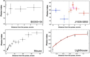
Yet another puzzle of pulsar tails is the very different dependences of their X-ray spectra on the distance from the pulsar along the tail (see figure 8). The rapid changes of photon index, likely due to synchrotron cooling, are seen in the tails of younger pulsars (e.g. J1747–2958, J1101–6101, and J0537–6910) while virtually no changes are seen in the tails of older pulsars (e.g. J1509–5850 and B0355 $+$
54). The different spectral evolution might be explained by different strength of magnetic field. The magnetic field strengths could be reduced by more efficient reconnection in the tail in the case of pulsars with a large angle between the spin axis and the velocity vector because larger angles may lead to a more tangled large-scale magnetic field in the tail. The continuing reconnection of magnetic fields in long tails could also lead to particle re-acceleration, which could help to explain the lack of softening in the X-ray spectra of the J1509–5850 and B0355
$+$
54). The different spectral evolution might be explained by different strength of magnetic field. The magnetic field strengths could be reduced by more efficient reconnection in the tail in the case of pulsars with a large angle between the spin axis and the velocity vector because larger angles may lead to a more tangled large-scale magnetic field in the tail. The continuing reconnection of magnetic fields in long tails could also lead to particle re-acceleration, which could help to explain the lack of softening in the X-ray spectra of the J1509–5850 and B0355 $+$
54 tails. In cases where the spin axis is nearly aligned with the magnetic dipole axis, reconnection may be delayed (because magnetic energy is not being efficiently converted to particle energy) until significant distortions or turbulence develop at larger distances down the tail (which may explain the lack of a ‘head’ in the X-ray images of J0357
$+$
54 tails. In cases where the spin axis is nearly aligned with the magnetic dipole axis, reconnection may be delayed (because magnetic energy is not being efficiently converted to particle energy) until significant distortions or turbulence develop at larger distances down the tail (which may explain the lack of a ‘head’ in the X-ray images of J0357 $+$
3205). A larger sample of bow shock PWNe is needed to probe these scenarios.
$+$
3205). A larger sample of bow shock PWNe is needed to probe these scenarios.
From (3.4) in § 3, it is possible to crudely estimate the average characteristic flow speed in the tail: $v_{\text{flow}}\sim l/t_{\text{syn}}$
, where
$v_{\text{flow}}\sim l/t_{\text{syn}}$
, where $l$
is the length of the X-ray tail. The bulk flow speeds estimated in this simplistic way are 2000, 3000, 3000, and
$l$
is the length of the X-ray tail. The bulk flow speeds estimated in this simplistic way are 2000, 3000, 3000, and ${>}1000~\text{km}~\text{s}^{-1}$
in the B0355
${>}1000~\text{km}~\text{s}^{-1}$
in the B0355 $+$
54, J1509–5850, J1101–6101 and the Mouse tails, respectivelyFootnote
12
. They are significantly higher that the pulsar speeds (with a possible exception of the very fast PSR J1101–6101).
$+$
54, J1509–5850, J1101–6101 and the Mouse tails, respectivelyFootnote
12
. They are significantly higher that the pulsar speeds (with a possible exception of the very fast PSR J1101–6101).
6 Misaligned outflows
In recent deep X-ray observations, a new type of structure has unexpectedly been discovered in some supersonic PWNe. Extended, elongated features, strongly misaligned with the pulsar’s direction of motion, are seen originating from the vicinity of four pulsars (see figure 9): the Guitar Nebula (PSR B2224 $+$
65; Hui & Becker Reference Hui and Becker2007), the Lighthouse PWN (PSR J1101–6101; Pavan et al.
Reference Pavan, Bordas, Pühlhofer, Filipović, De Horta, O’Brien, Balbo, Walter, Bozzo and Ferrigno2014, Reference Pavan, Pühlhofer, Bordas, Audard, Balbo, Bozzo, Eckert, Ferrigno, Filipović and Verdugo2016), the PWN of PSR J1509–5058 (Klingler et al.
Reference Klingler, Kargaltsev, Rangelov, Pavlov, Posselt and Ng2016a
), and the Mushroom PWN of PSR B0355
$+$
65; Hui & Becker Reference Hui and Becker2007), the Lighthouse PWN (PSR J1101–6101; Pavan et al.
Reference Pavan, Bordas, Pühlhofer, Filipović, De Horta, O’Brien, Balbo, Walter, Bozzo and Ferrigno2014, Reference Pavan, Pühlhofer, Bordas, Audard, Balbo, Bozzo, Eckert, Ferrigno, Filipović and Verdugo2016), the PWN of PSR J1509–5058 (Klingler et al.
Reference Klingler, Kargaltsev, Rangelov, Pavlov, Posselt and Ng2016a
), and the Mushroom PWN of PSR B0355 $+$
54 (Klingler et al.
Reference Klingler, Rangelov, Kargaltsev, Pavlov, Romani, Posselt, Slane, Temim, Ng and Bucciantini2016b
). Another, possibly similar, misaligned feature was reported for PSR J2055
$+$
54 (Klingler et al.
Reference Klingler, Rangelov, Kargaltsev, Pavlov, Romani, Posselt, Slane, Temim, Ng and Bucciantini2016b
). Another, possibly similar, misaligned feature was reported for PSR J2055 $+$
2539 based on XMM-Newton observations (Marelli et al.
Reference Marelli, Pizzocaro, De Luca, Gastaldello, Caraveo and Saz Parkinson2016b
). The misaligned orientation of these features is puzzling because, for a fast-moving pulsar, one would expect all of the PW to be confined within the tail (which three of the four PWNe exhibit as well). In principle, one could imagine a highly anisotropic wind with extremely strong polar outflows (jets) misaligned with the pulsar’s velocity vector. Such jets should be bent by the ram pressure of the oncoming ISM, with the bending length scale
$+$
2539 based on XMM-Newton observations (Marelli et al.
Reference Marelli, Pizzocaro, De Luca, Gastaldello, Caraveo and Saz Parkinson2016b
). The misaligned orientation of these features is puzzling because, for a fast-moving pulsar, one would expect all of the PW to be confined within the tail (which three of the four PWNe exhibit as well). In principle, one could imagine a highly anisotropic wind with extremely strong polar outflows (jets) misaligned with the pulsar’s velocity vector. Such jets should be bent by the ram pressure of the oncoming ISM, with the bending length scale $l_{b}\sim \unicode[STIX]{x1D709}_{j}{\dot{E}}/(cr_{j}\unicode[STIX]{x1D70C}v^{2}\sin \unicode[STIX]{x1D703})$
, where
$l_{b}\sim \unicode[STIX]{x1D709}_{j}{\dot{E}}/(cr_{j}\unicode[STIX]{x1D70C}v^{2}\sin \unicode[STIX]{x1D703})$
, where $\unicode[STIX]{x1D709}_{j}<1$
is the fraction of the spin-down power
$\unicode[STIX]{x1D709}_{j}<1$
is the fraction of the spin-down power ${\dot{E}}$
that goes into the jet,
${\dot{E}}$
that goes into the jet, $r_{j}$
is the jet radius, and
$r_{j}$
is the jet radius, and $\unicode[STIX]{x1D703}$
is the angle between the initial jet direction and the pulsar’s velocity. However, the bending length-scales are way too small compared to the lengths of the nearly straight misaligned features. For instance,
$\unicode[STIX]{x1D703}$
is the angle between the initial jet direction and the pulsar’s velocity. However, the bending length-scales are way too small compared to the lengths of the nearly straight misaligned features. For instance, $l_{b}\sim 0.065\unicode[STIX]{x1D709}_{j}(r_{j}/5.7\times 10^{16}~\text{cm})^{-1}n^{-1}(\sin \unicode[STIX]{x1D703})^{-1}(v/300~\text{km}~\text{s}^{-1})^{-2}$
pc for J1509–5850, while the observed length of the misaligned outflow is
$l_{b}\sim 0.065\unicode[STIX]{x1D709}_{j}(r_{j}/5.7\times 10^{16}~\text{cm})^{-1}n^{-1}(\sin \unicode[STIX]{x1D703})^{-1}(v/300~\text{km}~\text{s}^{-1})^{-2}$
pc for J1509–5850, while the observed length of the misaligned outflow is ${\sim}$
8 pc (for
${\sim}$
8 pc (for $d=3.8$
kpc; see Klingler et al.
Reference Klingler, Kargaltsev, Rangelov, Pavlov, Posselt and Ng2016a
for details). Therefore, it is difficult to explain the misaligned outflows with a hydrodynamic-type model.
$d=3.8$
kpc; see Klingler et al.
Reference Klingler, Kargaltsev, Rangelov, Pavlov, Posselt and Ng2016a
for details). Therefore, it is difficult to explain the misaligned outflows with a hydrodynamic-type model.
Chandra images of PWNe displaying misaligned outflows. The white arrows show the directions of pulsar proper motion, and the green arrow shows the bending in the Lighthouse Nebula outflow (inset). Chandra images of some of these objects are also shown in Reynolds et al. (Reference Reynolds, Pavlov, Kargaltsev, Klingler, Renaud and Mereghetti2017).

To interpret the first discovered misaligned outflow in the Guitar Nebula, Bandiera (Reference Bandiera2008) suggested that such structures can be formed in high- ${\mathcal{M}}$
pulsars when the gyro-radii of most energetic electrons,
${\mathcal{M}}$
pulsars when the gyro-radii of most energetic electrons, $r_{g}=\unicode[STIX]{x1D6FE}m_{e}c^{2}/eB_{\text{apex}}$
, are comparable to or exceed the stand-off distance of the bow shock apex,
$r_{g}=\unicode[STIX]{x1D6FE}m_{e}c^{2}/eB_{\text{apex}}$
, are comparable to or exceed the stand-off distance of the bow shock apex, $R_{h}=({\dot{E}}/4\unicode[STIX]{x03C0}cm_{p}nv^{2})^{1/2}$
(for isotropic wind), where
$R_{h}=({\dot{E}}/4\unicode[STIX]{x03C0}cm_{p}nv^{2})^{1/2}$
(for isotropic wind), where $B_{\text{apex}}$
is the magnetic field inside the PWN (between the contact discontinuity and termination shock) near the bow shock apex. Such particles cannot be contained within the bow shock, and can hence ‘leak’ into the ISM, where they diffuse along the ambient ISM magnetic field lines and radiate synchrotron photons. The Lorentz factors of escaping electrons, therefore, can be estimated as
$B_{\text{apex}}$
is the magnetic field inside the PWN (between the contact discontinuity and termination shock) near the bow shock apex. Such particles cannot be contained within the bow shock, and can hence ‘leak’ into the ISM, where they diffuse along the ambient ISM magnetic field lines and radiate synchrotron photons. The Lorentz factors of escaping electrons, therefore, can be estimated as $\unicode[STIX]{x1D6FE}\sim 2\times 10^{8}(E/1~\text{keV})^{1/2}(B_{\text{ISM}}/5~\unicode[STIX]{x03BC}\text{G})^{-1/2}$
, where
$\unicode[STIX]{x1D6FE}\sim 2\times 10^{8}(E/1~\text{keV})^{1/2}(B_{\text{ISM}}/5~\unicode[STIX]{x03BC}\text{G})^{-1/2}$
, where $B_{\text{ISM}}$
is the ambient magnetic field, and
$B_{\text{ISM}}$
is the ambient magnetic field, and $E$
is the synchrotron photon energy that reaches at least 8 keV for the Lighthouse, Guitar and J1509–5058 PWNe. From the escape condition,
$E$
is the synchrotron photon energy that reaches at least 8 keV for the Lighthouse, Guitar and J1509–5058 PWNe. From the escape condition, $r_{g}\gtrsim R_{h}$
, one can set an upper limit on the PWN field near the apex:
$r_{g}\gtrsim R_{h}$
, one can set an upper limit on the PWN field near the apex: $B_{\text{apex}}\lesssim 34(E/1~\text{keV})^{1/2}(B_{\text{ISM}}/5~\unicode[STIX]{x03BC}\text{G})^{-1/2}(R_{h}/10^{16}~\text{cm})^{-1}~\unicode[STIX]{x03BC}\text{G}$
, if
$B_{\text{apex}}\lesssim 34(E/1~\text{keV})^{1/2}(B_{\text{ISM}}/5~\unicode[STIX]{x03BC}\text{G})^{-1/2}(R_{h}/10^{16}~\text{cm})^{-1}~\unicode[STIX]{x03BC}\text{G}$
, if $R_{h}$
is directly measured or estimated from the equation given above.
$R_{h}$
is directly measured or estimated from the equation given above.
It is important to stress that in this scenario the misaligned outflows are an entirely kinetic phenomenon, which makes them very different from the pressure-confined jets of tails. The observed appearances of the misaligned outflows should reflect the ambient ISM structureFootnote 13 illuminated by synchrotron emission from the leaked PW particles. In the discussed scenario, the misaligned structures are expected to move with the particle injection site (SPWN apex) which moves with the pulsar.
The Bandiera (Reference Bandiera2008) scenario was challenged by recent deep Chandra observations of the Lighthouse PWN where the misaligned outflow appears to bend around the pulsar (as indicated by the green arrow in the inset image in the top right panel of figure 9). Although the distortion of the external (ISM) field can be expected if a magnetized object is moving through the ISM (‘magnetic draping’; Lyutikov Reference Lyutikov2006 and Dursi & Pfrommer Reference Dursi and Pfrommer2008), this should not be happening outside the forward shock region where the ISM ‘does not know’ about the incoming object yet. Another difficulty with this scenario is that most of these misaligned outflows (with a possible exception of a very faint one associated with B0355 $+$
54) are strongly asymmetric (i.e. they appear much brighter and longer on one side of the pulsar).
$+$
54) are strongly asymmetric (i.e. they appear much brighter and longer on one side of the pulsar).
7 Forward shock emission
If the local ISM contains neutral Hydrogen, collisional excitation and charge exchange in the forward shock can cause the shocked ISM to emit in $H\unicode[STIX]{x1D6FC}$
leading to formation of an
$H\unicode[STIX]{x1D6FC}$
leading to formation of an $H\unicode[STIX]{x1D6FC}$
bow shock. To date, bow-shaped
$H\unicode[STIX]{x1D6FC}$
bow shock. To date, bow-shaped $H\unicode[STIX]{x1D6FC}$
nebulae have been detected around only eight rotation-powered pulsars (see table 2 and Brownsberger & Romani Reference Brownsberger and Romani2014). A possible explanation for the scarcity of
$H\unicode[STIX]{x1D6FC}$
nebulae have been detected around only eight rotation-powered pulsars (see table 2 and Brownsberger & Romani Reference Brownsberger and Romani2014). A possible explanation for the scarcity of $H\unicode[STIX]{x1D6FC}$
bow shocks is a high degree of ionization of the ambient medium ahead of the pulsar, which might be caused by pre-ionization of the ISM by radiation from the pulsar and/or the X-ray PWN.
$H\unicode[STIX]{x1D6FC}$
bow shocks is a high degree of ionization of the ambient medium ahead of the pulsar, which might be caused by pre-ionization of the ISM by radiation from the pulsar and/or the X-ray PWN.
One of the first $H\unicode[STIX]{x1D6FC}$
pulsar bow shocks was detected by Bell, Bailes & Bessell (Reference Bell, Bailes and Bessell1993) ahead of the binary millisecond (recycled) pulsar J0437–4715. PSR J0437–4715 is the closest known pulsar,
$H\unicode[STIX]{x1D6FC}$
pulsar bow shocks was detected by Bell, Bailes & Bessell (Reference Bell, Bailes and Bessell1993) ahead of the binary millisecond (recycled) pulsar J0437–4715. PSR J0437–4715 is the closest known pulsar, $d=156.8\pm 0.2$
pc (Reardon et al.
Reference Reardon, Hobbs, Coles, Levin, Keith, Bailes, Bhat, Burke-Spolaor, Dai and Kerr2016), with an accurately measured proper motion corresponding to the transverse velocity
$d=156.8\pm 0.2$
pc (Reardon et al.
Reference Reardon, Hobbs, Coles, Levin, Keith, Bailes, Bhat, Burke-Spolaor, Dai and Kerr2016), with an accurately measured proper motion corresponding to the transverse velocity $v_{\bot }=104.1\pm 0.2~\text{km}~\text{s}^{-1}$
(Deller et al.
Reference Deller, Verbiest, Tingay and Bailes2008). It has a period of 5.8 ms and a spin-down power
$v_{\bot }=104.1\pm 0.2~\text{km}~\text{s}^{-1}$
(Deller et al.
Reference Deller, Verbiest, Tingay and Bailes2008). It has a period of 5.8 ms and a spin-down power ${\dot{E}}=2.9\times 10^{33}I_{45}~\text{erg}~\text{s}^{-1}$
(corrected for the Shklovskii effect;
${\dot{E}}=2.9\times 10^{33}I_{45}~\text{erg}~\text{s}^{-1}$
(corrected for the Shklovskii effect; $I_{45}$
is the neutron star moment of inertia in units of
$I_{45}$
is the neutron star moment of inertia in units of $10^{45}~\text{g}~\text{cm}^{2}$
). Its
$10^{45}~\text{g}~\text{cm}^{2}$
). Its $H\unicode[STIX]{x1D6FC}$
bow shock shows a symmetric structure with a stand-off distance of approximately
$H\unicode[STIX]{x1D6FC}$
bow shock shows a symmetric structure with a stand-off distance of approximately $10^{\prime \prime }$
(
$10^{\prime \prime }$
( $2.3\times 10^{16}$
cm) between the pulsar and the bow shock apex (see figure 10).
$2.3\times 10^{16}$
cm) between the pulsar and the bow shock apex (see figure 10).
The J0437–4715 bow shock is the first one detected in far-UV, thanks to the pulsar proximity and deep observations with the Hubble Space Telescope. The far-UV images reveal a bow-like structure positionally coincident with the $H\unicode[STIX]{x1D6FC}$
bow shock (figure 10). The measurements in broad F125LP and F140LP filters (wavelength bands are 1250–2000 Å and 1350–2000 Å, respectively) do not allow us to establish the spectral model. The existing data are consistent with both a simple power-law spectrum, which could be continuum synchrotron emission from relativistic electrons trapped in the forward shock region (Bykov et al.
Reference Bykov, Amato, Petrov, Krassilchtchikov and Levenfish2017), and the collisionless plasma emission (spectral lines plus continuum) from the ISM matter compressed and heated in the forward shock region (Bykov et al.
Reference Bykov, Malkov, Raymond, Krassilchtchikov and Vladimirov2013).
$H\unicode[STIX]{x1D6FC}$
bow shock (figure 10). The measurements in broad F125LP and F140LP filters (wavelength bands are 1250–2000 Å and 1350–2000 Å, respectively) do not allow us to establish the spectral model. The existing data are consistent with both a simple power-law spectrum, which could be continuum synchrotron emission from relativistic electrons trapped in the forward shock region (Bykov et al.
Reference Bykov, Amato, Petrov, Krassilchtchikov and Levenfish2017), and the collisionless plasma emission (spectral lines plus continuum) from the ISM matter compressed and heated in the forward shock region (Bykov et al.
Reference Bykov, Malkov, Raymond, Krassilchtchikov and Vladimirov2013).
Analysing a subset of archival Chandra ACIS data, Rangelov et al. (Reference Rangelov, Pavlov, Kargaltsev, Durant, Bykov and Krassilchtchikov2016) also found a faint extended X-ray emission ahead of the pulsar but well within the $H\unicode[STIX]{x1D6FC}$
bow shock (figure 10). This emission was tentatively interpreted as an X-ray PWN of J0437. The morphology of the PWN is unusual compared to other supersonic PWNe in the sense that the X-ray emission is seen only ahead of the moving pulsar, being confined to a relatively narrow region. However, such a bright region of emission ahead of the pulsar consistent with simulated synchrotron maps of the bow shock PWNe (see figure 4 from Bucciantini et al.
Reference Bucciantini, Amato and Del Zanna2005). These regions may simply be unresolvable in other, more remote PWNe, but due to the proximity of J0437, Chandra observations can probe shocked PW X-ray emission on much smaller spatial scales.
$H\unicode[STIX]{x1D6FC}$
bow shock (figure 10). This emission was tentatively interpreted as an X-ray PWN of J0437. The morphology of the PWN is unusual compared to other supersonic PWNe in the sense that the X-ray emission is seen only ahead of the moving pulsar, being confined to a relatively narrow region. However, such a bright region of emission ahead of the pulsar consistent with simulated synchrotron maps of the bow shock PWNe (see figure 4 from Bucciantini et al.
Reference Bucciantini, Amato and Del Zanna2005). These regions may simply be unresolvable in other, more remote PWNe, but due to the proximity of J0437, Chandra observations can probe shocked PW X-ray emission on much smaller spatial scales.
The second bow shock detected in far-UV is associated with the solitary millisecond PSR J2124–3358 (Rangelov et al.
Reference Rangelov, Pavlov, Kargaltsev, Reisenegger, Guillot, van Kerkwijk and Reyes2017). This pulsar has a period of 4.93 ms and a spin-down power ${\dot{E}}=6.8\times 10^{33}I_{45}~\text{erg}~\text{s}^{-1}$
. It is at a distance
${\dot{E}}=6.8\times 10^{33}I_{45}~\text{erg}~\text{s}^{-1}$
. It is at a distance $d=410_{-70}^{+90}$
pc, its proper motion corresponds to
$d=410_{-70}^{+90}$
pc, its proper motion corresponds to $v_{\bot }=101.2\pm 0.8$
km, at
$v_{\bot }=101.2\pm 0.8$
km, at $d=410$
pc (Reardon et al.
Reference Reardon, Hobbs, Coles, Levin, Keith, Bailes, Bhat, Burke-Spolaor, Dai and Kerr2016). The shape of its far-UV bow shock matches well the
$d=410$
pc (Reardon et al.
Reference Reardon, Hobbs, Coles, Levin, Keith, Bailes, Bhat, Burke-Spolaor, Dai and Kerr2016). The shape of its far-UV bow shock matches well the $H\unicode[STIX]{x1D6FC}$
bow shock, which suggests that the far-UV emission comes from the forward shock region. The poor statistics once again prevents us from discriminating between the power-law and collisionless shock plasma emission models. A sensitive slit or integral field spectroscopy would enable further progress in understanding the nature of far-UV emission from the pulsar bow shocks.
$H\unicode[STIX]{x1D6FC}$
bow shock, which suggests that the far-UV emission comes from the forward shock region. The poor statistics once again prevents us from discriminating between the power-law and collisionless shock plasma emission models. A sensitive slit or integral field spectroscopy would enable further progress in understanding the nature of far-UV emission from the pulsar bow shocks.
Hui & Becker (Reference Hui and Becker2006) reported an X-ray PWN associated with J2124–3358. It was detected with both XMM-Newton and Chandra, but only Chandra was able to resolve the nebula into a one-sided narrow structure, which appears to be projected inside the observed $H\unicode[STIX]{x1D6FC}$
-far-UV bow shock (see figure 11). The X-ray emission extends northwest from the pulsar for
$H\unicode[STIX]{x1D6FC}$
-far-UV bow shock (see figure 11). The X-ray emission extends northwest from the pulsar for ![]() Hui & Becker (Reference Hui and Becker2006) modelled the spectrum of the emission with a power-law model with photon index
Hui & Becker (Reference Hui and Becker2006) modelled the spectrum of the emission with a power-law model with photon index $\unicode[STIX]{x1D6E4}=2.2\pm 0.4$
.
$\unicode[STIX]{x1D6E4}=2.2\pm 0.4$
.
(a) Shows an $H\unicode[STIX]{x1D6FC}$
image of PSR J0437–4715 obtained with the SOAR telescope (Brownsberger & Romani Reference Brownsberger and Romani2014). (b) Shows a Chandra ACIS-S3 image. The magenta contours delineate the source and background extraction regions used for the extended emission analysis; the white contour, coinciding with that in (a), shows the position of the
$H\unicode[STIX]{x1D6FC}$
image of PSR J0437–4715 obtained with the SOAR telescope (Brownsberger & Romani Reference Brownsberger and Romani2014). (b) Shows a Chandra ACIS-S3 image. The magenta contours delineate the source and background extraction regions used for the extended emission analysis; the white contour, coinciding with that in (a), shows the position of the $H\unicode[STIX]{x1D6FC}$
bow shock apex. (c,d) Show far-UV images from two different observations (dates are labelled) and different filters (also labelled). The non-uniform background prominent in the far-UV images is due to the ‘thermal glow’ of the detector. The extended ‘blob’ of unknown nature is seen in (c).
$H\unicode[STIX]{x1D6FC}$
bow shock apex. (c,d) Show far-UV images from two different observations (dates are labelled) and different filters (also labelled). The non-uniform background prominent in the far-UV images is due to the ‘thermal glow’ of the detector. The extended ‘blob’ of unknown nature is seen in (c). $H\unicode[STIX]{x1D6FC}$
bow shock contours (based on the SOAR image) are shown in (d). North is up, East is to the left. The images are taken from Rangelov et al. (Reference Rangelov, Pavlov, Kargaltsev, Durant, Bykov and Krassilchtchikov2016).
$H\unicode[STIX]{x1D6FC}$
bow shock contours (based on the SOAR image) are shown in (d). North is up, East is to the left. The images are taken from Rangelov et al. (Reference Rangelov, Pavlov, Kargaltsev, Durant, Bykov and Krassilchtchikov2016).

In addition to eight rotation-powered pulsars, bow-shaped $H\unicode[STIX]{x1D6FC}$
emission has been detected around the radio-quiet isolated neutron star RX J1856.5–3754 (van Kerkwijk & Kulkarni Reference van Kerkwijk and Kulkarni2001). It belongs to the class of neutron stars that do not show any signatures of magnetospheric activity (e.g. non-thermal X-ray emission or radio/
$H\unicode[STIX]{x1D6FC}$
emission has been detected around the radio-quiet isolated neutron star RX J1856.5–3754 (van Kerkwijk & Kulkarni Reference van Kerkwijk and Kulkarni2001). It belongs to the class of neutron stars that do not show any signatures of magnetospheric activity (e.g. non-thermal X-ray emission or radio/ $\unicode[STIX]{x1D6FE}$
-ray pulsations; see Kaplan et al. (Reference Kaplan, Kamble, van Kerkwijk and Ho2011) and references therein). In this case the
$\unicode[STIX]{x1D6FE}$
-ray pulsations; see Kaplan et al. (Reference Kaplan, Kamble, van Kerkwijk and Ho2011) and references therein). In this case the $H\unicode[STIX]{x1D6FC}$
emission may represent a photoionization nebula rather than a bow shock (van Kerkwijk & Kulkarni Reference van Kerkwijk and Kulkarni2001). For this reason we do not include RX J1856.5–3754 in tables 1 and 2.
$H\unicode[STIX]{x1D6FC}$
emission may represent a photoionization nebula rather than a bow shock (van Kerkwijk & Kulkarni Reference van Kerkwijk and Kulkarni2001). For this reason we do not include RX J1856.5–3754 in tables 1 and 2.
(a) Shows a far-UV image of the PSR J2124–3358 vicinity obtained with the Hubble Space Telescope ACS/SBC F125LP filter. The pulsar and its direction of motion are shown with white circle and arrow. (b) Shows the SOAR $H\unicode[STIX]{x1D6FC}$
image; ‘X’ marks the position of the pulsar. (c) Shows the Chandra ACIS image in 0.5–7 keV. All images are to the same scale. North is up, and East to the left. The images are taken from Rangelov et al. (Reference Rangelov, Pavlov, Kargaltsev, Reisenegger, Guillot, van Kerkwijk and Reyes2017).
$H\unicode[STIX]{x1D6FC}$
image; ‘X’ marks the position of the pulsar. (c) Shows the Chandra ACIS image in 0.5–7 keV. All images are to the same scale. North is up, and East to the left. The images are taken from Rangelov et al. (Reference Rangelov, Pavlov, Kargaltsev, Reisenegger, Guillot, van Kerkwijk and Reyes2017).
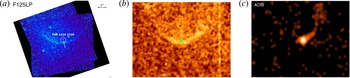
8 Conclusions
SPWNe exhibit a number of interesting properties providing insight into the structures of neutron star magnetospheres, winds and pulsar viewing geometry, as well as into the physics of collisionless shocks and supernova explosions. Some of these properties became apparent only from deep Chandra and Hubble Space Telescope observations:
-
(i) Very long (up to 8 pc) X-ray tails have been detected behind a few pulsars. In some cases the X-ray tails are accompanied by even longer radio tails. None of these long tails are seen in TeV.
-
(ii) Some of the tails exhibit very rapid spectral softening (cooling) with increasing distance from the pulsar (e.g. the Mouse and Lighthouse PWNe), while others show no evidence of cooling (e.g. J1509–5850).
-
(iii) When resolved in X-rays, the SPWN head morphologies can differ drastically. There can be ‘filled’, ‘empty’, and very dim (of absent) SPWN heads. The differences can be linked to the geometry of the pulsar magnetosphere and to the orientation of pulsar’s spin axis with respect to the observer’s line of sight.
-
(iv) There is a growing number of SPWNe with misaligned outflows which are likely produced by most energetic particles leaking from the SPWN apex. However, there are some unsolved puzzles in this scenario.
-
(v) Far-UV emission from two $H\unicode[STIX]{x1D6FC}$
bow shocks has been recently discovered, likely produced by heated shocked ISM.
$H\unicode[STIX]{x1D6FC}$
bow shocks has been recently discovered, likely produced by heated shocked ISM.

Although a general, qualitative picture of PWNe created by supersonically moving pulsars is more or less clear, there remain a number of open questions.
-
(i) Why are some SPWN heads very faint in X-rays? Are they simply too compact to be resolved from the pulsar?
-
(ii) Why do X-ray spectra of some tails remain hard at large distances from the pulsar?
-
(iii) What are particle acceleration mechanisms in SPWNe, and is there in-situ acceleration outside the termination shock?
-
(iv) How some of the tails remain so well collimated for such long distances?
-
(v) What is the nature of the misaligned outflows? Why are they so asymmetric?
-
(vi) Are the morphologies of X-ray PWN heads, PWN radiative efficiencies, and PWN spectra uniquely determined by mutual orientations of the line of sight, pulsar’s velocity, spin and magnetic axis?
-
(vii) Are the SPWNe intrinsically fainter in TeV
$\unicode[STIX]{x1D6FE}$
-rays compared to PWNe inside the SNRs?

To answer these and other questions, detailed studies of a larger sample of SPWNe must be supplemented by more realistic models.
Acknowledgements
This work was partly supported by the NASA through Chandra Awards GO3-14057 and G03-14082 issued by the Chandra X-ray Observatory Center, which is operated by the Smithsonian Astrophysical Observatory for and on behalf of the NASA under contract NAS8-03060. It was also supported by grants GO-12917 and GO-13783 from the Space Telescope Science Institute, which is operated by Association of Universities for Research in Astronomy, Inc. under NASA contract NAS 5-26555. We thank I. Volkov for discussions and help with the figures.


