


1. Introduction
An ice shelf is a floating extension of a continental ice sheet, formed where glacial ice flows from land into the ocean. These thick and expansive ice bodies are a key feature of Antarctica and parts of Greenland (Thomas Reference Thomas1979). Because they are attached to grounded ice, ice shelves play an important role in slowing the flow of inland ice towards the sea. By providing a buttressing effect, they help to limit the movement of glaciers and ice streams behind them, in turn reducing the amount of land ice entering the ocean, and helping to mitigate sea-level rise (Thomas Reference Thomas1979). When ice shelves break up, this stabilising effect is lost. The glaciers that they previously restrained can accelerate, increasing the discharge of ice into the ocean, and contributing to rising sea levels (Vaughan Reference Vaughan1995). Historical events, such as the collapse of the Larsen B Ice Shelf in 2002 and the Wilkins Ice Shelf in 1998, have been linked to the subsequent acceleration of ice discharge into the ocean (Scambos et al. Reference Scambos, Hulbe, Fahnestock and Bohlander2000, Reference Scambos, Bohlander, Shuman and Skvarca2004), underscoring the need to understand the processes that undermine ice shelf stability. Several processes contribute to ice shelf break-up, including both climatic and mechanical factors. Climatic drivers, such as warming air and ocean temperatures, progressively weaken the ice shelves over time (Scambos et al. Reference Scambos, Hulbe, Fahnestock and Bohlander2000). Satellite observations show that many West Antarctic ice shelves are rapidly thinning, primarily due to basal melting caused by intrusions of warm Circumpolar Deep Water (Paolo, Fricker & Padman Reference Paolo, Fricker and Padman2015). This thinning reduces their buttressing capacity and increases the risk of break-up. Mechanical processes also play a significant role in ice shelf failure. For example, tidal flexure generates bending stresses near grounding lines (Vaughan Reference Vaughan1995), and ocean waves can excite vibrations that promote cracking (Holdsworth & Glynn Reference Holdsworth and Glynn1981). In particular, long-period ocean gravity waves can induce low-frequency Rayleigh–Lamb flexural vibrations that travel deep into the ice shelf and impose mechanical stresses over large distances (MacAyeal et al. Reference MacAyeal2006; Bromirski, Sergienko & MacAyeal Reference Bromirski, Sergienko and MacAyeal2010; Sergienko Reference Sergienko2010; Bromirski et al. Reference Bromirski, Diez, Gerstoft, Stephen, Bolmer, Wiens, Aster and Nyblade2015). Detailed observations from the Ross Ice Shelf show that infragravity waves from distant storms transmit significant energy into the ice, generating vibrations that may propagate and extend fractures within the ice body (MacAyeal et al. Reference MacAyeal2006; Bromirski et al. Reference Bromirski, Diez, Gerstoft, Stephen, Bolmer, Wiens, Aster and Nyblade2015). These vibrations are believed to contribute to structural weakening and the eventual break-up of ice shelves (Bromirski et al. Reference Bromirski, Diez, Gerstoft, Stephen, Bolmer, Wiens, Aster and Nyblade2015).
Several studies have employed linear hydroelastic models to investigate wave–ice shelf interactions, treating the ice shelf as a thin floating elastic plate subjected to ocean wave forcing (Meylan et al. Reference Meylan, Bennetts, Hosking and Catt2017; Kalyanaraman et al. Reference Kalyanaraman, Bennetts, Lamichhane and Meylan2019; Papathanasiou, Karperaki & Belibassakis Reference Papathanasiou, Karperaki and Belibassakis2019). If the wavelength is long compared to the depth of the fluid, then the modelling can be further simplified by treating the fluid using shallow-water wave theory (Sergienko Reference Sergienko2013; Bennetts & Meylan Reference Bennetts and Meylan2021; McNeil & Meylan Reference McNeil and Meylan2023; Alshahrani, Meylan & Wilks Reference Alshahrani, Meylan and Wilks2024). Using this approach, Sergienko (Reference Sergienko2013) studied a system combining an infinitely long ice shelf with the ocean cavity beneath it. The study solved for the natural frequencies and modes of vibration, and showed that these were consistent with the vibration frequencies observed in real ice shelves. Later, Bennetts & Meylan (Reference Bennetts and Meylan2021) extended the model to account for finite ice shelf length, variable thickness and variable bathymetry, and studied the shelf’s resonant behaviour using complex resonance analysis. McNeil & Meylan (Reference McNeil and Meylan2023) developed and solved a time-dependent model of wave-induced vibration of a semi-infinite ice shelf using the same shallow-water thin plate approximation coupling. Recently, Aljabri & Meylan (Reference Aljabri and Meylan2024) developed a time-domain model to simulate the vibrations of an ice shelf modelled as a two-dimensional elastic plate floating in shallow water. Their study investigated the effects of different boundary conditions (no flux and no pressure) and provided insight into the complex modal behaviour and transient dynamics of intact ice shelves. Alshammari & Meylan (Reference Alshammari and Meylan2025) extended the linear hydroelastic model to ice shelves containing cracks by introducing cracked plate boundary conditions. By demonstrating how cracks influence the mode shapes and transient vibration patterns, their work marked a first step towards simulating ice shelf crack formation.
These earlier studies have been unable to be extended to investigate sequential break-up: a proposed mechanism for ice shelf break-up where individual ice shelf fragments detach in a series of discrete events, occurring when and where bending stresses surpass some critical threshold. To construct a sequential break-up model in this framework: (i) the thin plate approximation/shallow-water model of the ice shelf/ocean system must be extended to the case where one or more ice shelf fragments are detached from the original ice shelf, and (ii) the mathematical framework must be extended to an initial boundary value problem, so that simulation of the ice shelf can be resumed after a fracture event. Milestone (i) was addressed by Alshahrani et al. (Reference Alshahrani, Meylan and Wilks2024), who studied wave scattering by a finite number of finite ice shelf fragments in front of a semi-infinite ice shelf. Using the transfer matrix method, they solved the multiple scattering problem in the frequency domain, and extended their results to the time domain. However, the treatment of the time domain in the model of Alshahrani et al. (Reference Alshahrani, Meylan and Wilks2024) was limited, as it did not allow the solution of initial–boundary value problems. The present study makes progress towards this gap (i.e. milestone (ii)) by developing a full time-domain model for a fully bounded ice shelf to analyse its transient vibrational behaviour and break-up mechanisms. It is worth mentioning the recent work of Mokus & Montiel (Reference Mokus and Montiel2022), who studied sea ice break-up induced by waves in a finite-depth fluid model. They used a frequency domain analysis of sequential break-up to predict floe size distributions resulting from different forcing scenarios. However, the underlying mechanism is likely better represented by a time-dependent model, so the validity of their frequency domain analysis of sea ice break-up is unknown. While our work is primarily motivated by the problem of ice shelf break-up, it could be extended to sea ice break-up because the underlying models are similar.
The remainder of this paper is organised as follows. In § 2, we present the mathematical formulation of the problem, modelling the ice shelf–ocean system through the coupling of Kirchhoff–Love plate theory with linear shallow-water wave theory. Section 3 outlines the approach for obtaining the model solution, including the reduction to a nonlinear matrix eigenvalue problem, which is solved numerically to determine the modes and vibration frequencies of the coupled system. These modes are then used to construct the time-domain solution in § 4 using a spectral method. Numerical results illustrating the dynamic behaviour of the bounded ice shelf are presented in § 5. A brief summary is given in § 6.
2. Mathematical model
We consider Kirchhoff–Love plate theory with no variation in $y$
(an infinitely wide plate), so the problem is one-dimensional and equivalent to Euler–Bernoulli beam theory, with the flexural rigidity scaled by
$y$
(an infinitely wide plate), so the problem is one-dimensional and equivalent to Euler–Bernoulli beam theory, with the flexural rigidity scaled by $1-\nu ^{2}$
, where
$1-\nu ^{2}$
, where $\nu$
is Poisson’s ratio. We work on a one-dimensional bounded domain
$\nu$
is Poisson’s ratio. We work on a one-dimensional bounded domain $x \in [-L,L]$
: the left-hand half,
$x \in [-L,L]$
: the left-hand half, $x \in (-L,0)$
, contains a fluid with a free surface, and the right-hand half,
$x \in (-L,0)$
, contains a fluid with a free surface, and the right-hand half, $x \in (0,L)$
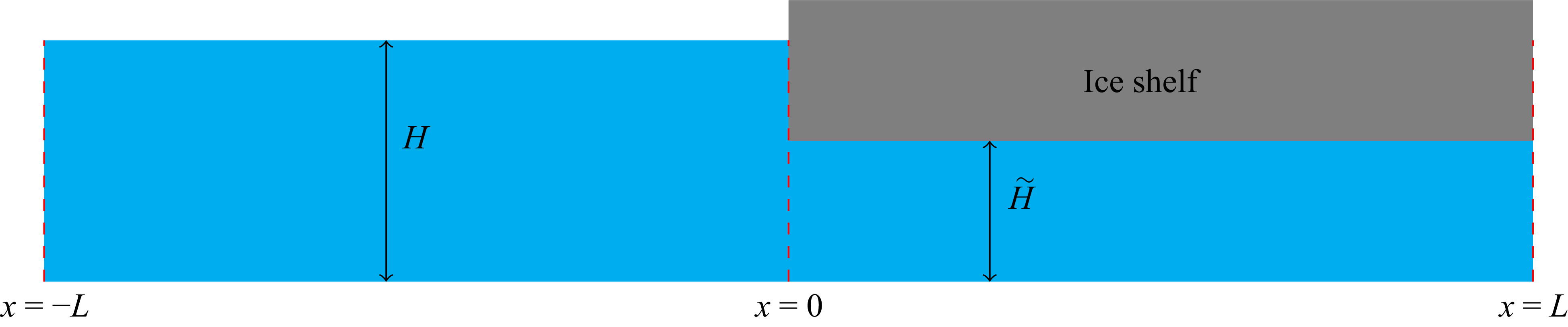
, contains a fluid overlain by an ice shelf. The thin plate approximation adopted here is consistent with the classical framework for floating-ice flexure (e.g. Timoshenko & Goodier Reference Timoshenko and Goodier1934; Sergienko Reference Sergienko2013). For simplicity, we assume that the ice shelf spans exactly half the domain, though this assumption can be readily extended to more general cases. The fluid and ice shelf are assumed to have constant depth and constant thickness, respectively. We note that in reality, the ice shelf has variable properties in depth (as well as variation in thickness), and all parameters should be seen as representative averages. We also apply the assumption of shallow water, which requires the length scale of any motion to be much greater than the water depth and the ice shelf thickness (since we apply the shallow-water assumption in the open water region). Within the shallow-water framework, the motion of the system is described by the vertical displacement
$x \in (0,L)$
, contains a fluid overlain by an ice shelf. The thin plate approximation adopted here is consistent with the classical framework for floating-ice flexure (e.g. Timoshenko & Goodier Reference Timoshenko and Goodier1934; Sergienko Reference Sergienko2013). For simplicity, we assume that the ice shelf spans exactly half the domain, though this assumption can be readily extended to more general cases. The fluid and ice shelf are assumed to have constant depth and constant thickness, respectively. We note that in reality, the ice shelf has variable properties in depth (as well as variation in thickness), and all parameters should be seen as representative averages. We also apply the assumption of shallow water, which requires the length scale of any motion to be much greater than the water depth and the ice shelf thickness (since we apply the shallow-water assumption in the open water region). Within the shallow-water framework, the motion of the system is described by the vertical displacement $W(x,t)$
and the fluid velocity potential
$W(x,t)$
and the fluid velocity potential $\varPhi (x,t)$
. In particular, the vertical displacement
$\varPhi (x,t)$
. In particular, the vertical displacement $W(x,t)$
represents the displacement of the free surface in the ocean region
$W(x,t)$
represents the displacement of the free surface in the ocean region $(-L,0)$
, and the vertical motion of the ice shelf in the covered region
$(-L,0)$
, and the vertical motion of the ice shelf in the covered region $(0,L)$
. Unlike Meylan (Reference Meylan2002), who considered an elastic plate in an infinite domain, we study an ice shelf in a finite domain. This choice yields a discrete eigenfrequency spectrum, which makes resonances straightforward to identify and resolve; in contrast, the infinite-domain setting leads to a continuous spectrum and scattering resonances that are much harder to isolate numerically. In this framework,
$(0,L)$
. Unlike Meylan (Reference Meylan2002), who considered an elastic plate in an infinite domain, we study an ice shelf in a finite domain. This choice yields a discrete eigenfrequency spectrum, which makes resonances straightforward to identify and resolve; in contrast, the infinite-domain setting leads to a continuous spectrum and scattering resonances that are much harder to isolate numerically. In this framework, $W$
and
$W$
and $\varPhi$
satisfy the following coupled system of partial differential equations derived from shallow-water wave theory and thin plate approximation (Meylan Reference Meylan2002):
$\varPhi$
satisfy the following coupled system of partial differential equations derived from shallow-water wave theory and thin plate approximation (Meylan Reference Meylan2002):
 \begin{align} D \partial _x^4 W +\rho _I h \partial _t^2 W+\rho _w g W&=- \rho _w \partial _t \varPhi,\quad x\in (0,L), \end{align}
 \begin{align} g W &= -\partial _t\varPhi,\qquad\, x\in (-L,0), \end{align}
 \begin{align} \partial _x^2 \varPhi &= -\frac {1}{H}\, \partial _t\! W,\quad x\in (-L,0), \end{align}
 \begin{align} \partial _x^2 \varPhi &= -\frac {1}{\widetilde {H}}\, \partial _t\! W,\quad x\in (0,L), \end{align}
where $D= {E h^3}/{12(1-\nu ^2)}$
is the ice shelf’s flexural rigidity. Moreover,
$D= {E h^3}/{12(1-\nu ^2)}$
is the ice shelf’s flexural rigidity. Moreover, $\rho _w$
and
$\rho _w$
and $\rho _I$
are the densities of water and ice, respectively, which we assume to be
$\rho _I$
are the densities of water and ice, respectively, which we assume to be $\rho _w=1025$
kg m
$\rho _w=1025$
kg m $^{-3}$
and
$^{-3}$
and $\rho _I=922.5$
kg m
$\rho _I=922.5$
kg m $^{-3}$
. The thickness of the ice shelf is denoted
$^{-3}$
. The thickness of the ice shelf is denoted $h$
, and the depth of the water is denoted
$h$
, and the depth of the water is denoted $H$
, which implies that the vertical distance between the submerged face of the ice shelf and the seabed (denoted
$H$
, which implies that the vertical distance between the submerged face of the ice shelf and the seabed (denoted $\widetilde {H}$
) can be computed as
$\widetilde {H}$
) can be computed as $\widetilde {H}=H-( {\rho _I}/{\rho _w}) h$
. Moreover,
$\widetilde {H}=H-( {\rho _I}/{\rho _w}) h$
. Moreover, $E$
is the Young’s modulus of the ice shelf, which we take to be
$E$
is the Young’s modulus of the ice shelf, which we take to be $11$
GPa, and the Poisson’s ratio
$11$
GPa, and the Poisson’s ratio $\nu$
is taken to be 0.33. Acceleration due to gravity is denoted
$\nu$
is taken to be 0.33. Acceleration due to gravity is denoted $g=9.81$
m s
$g=9.81$
m s $^{-2}$
, and the geometry of the problem is illustrated in figure 1.
$^{-2}$
, and the geometry of the problem is illustrated in figure 1.
Schematic of the problem geometry. The domain consists of a bounded ice shelf of length $L$
above a fluid-containing sub-shelf cavity, with a bounded open-water region to the left of the shelf. The coordinate
$L$
above a fluid-containing sub-shelf cavity, with a bounded open-water region to the left of the shelf. The coordinate $x=0$
marks the seaward edge of the ice shelf, while
$x=0$
marks the seaward edge of the ice shelf, while $x=L$
denotes its land-connected edge.
$x=L$
denotes its land-connected edge.

Note that (2.1a
) would be equivalent to (2.1b
) if $D$
and
$D$
and $\rho _Ih$
were zero. We specify the following initial conditions at time
$\rho _Ih$
were zero. We specify the following initial conditions at time $t = 0$
:
$t = 0$
:
 \begin{align} W(x, 0) = f(x), \end{align}
 \begin{align} \frac {\partial\! W}{\partial t}(x, 0) = g(x). \end{align}
At the left-hand boundary ( $x=-L$
), we assume no flux into the fluid:
$x=-L$
), we assume no flux into the fluid:
 \begin{align} \frac {\partial \varPhi }{\partial x}\bigg |_{x=-L} = 0. \end{align}
At the interface $x = 0$
between the open water and the ice shelf, two matching conditions and two boundary conditions are applied to ensure appropriate physical behaviour. The matching conditions at
$x = 0$
between the open water and the ice shelf, two matching conditions and two boundary conditions are applied to ensure appropriate physical behaviour. The matching conditions at $x=0$
, which enforce continuity of pressure and continuity of horizontal flux, are
$x=0$
, which enforce continuity of pressure and continuity of horizontal flux, are
 \begin{align} \varPhi (0^-) &= \varPhi (0^+), \end{align}
 \begin{align} H \frac {\partial \varPhi }{\partial x}\bigg |_{x=0^-} &= \widetilde {H} \frac {\partial \varPhi }{\partial x}\bigg |_{x=0^+}, \end{align}
respectively. The ice shelf has a free edge at $x = 0$
, meaning that the bending moment and shear force vanish, implying
$x = 0$
, meaning that the bending moment and shear force vanish, implying
 \begin{align} \frac {\partial ^4 \varPhi }{\partial x^4}\bigg |_{x=0} = 0, \end{align}
 \begin{align} \frac {\partial ^5 \varPhi }{\partial x^5}\bigg |_{x=0} = 0, \end{align}
respectively. At the right-hand boundary $x = L$
, the ice shelf is treated as a clamped elastic plate, and there is assumed to be no horizontal fluid flux in the sub-ice-shelf cavity, yielding the following three boundary conditions:
$x = L$
, the ice shelf is treated as a clamped elastic plate, and there is assumed to be no horizontal fluid flux in the sub-ice-shelf cavity, yielding the following three boundary conditions:
 \begin{align} \frac {\partial \varPhi }{\partial x}\bigg |_{x=L} = 0, \end{align}
 \begin{align} \frac {\partial ^2 \varPhi }{\partial x^2}\bigg |_{x=L} = 0, \end{align}
 \begin{align} \frac {\partial ^3 \varPhi }{\partial x^3}\bigg |_{x=L} = 0. \end{align}
These initial and boundary conditions fully specify the problem in the time domain. We note that treating the grounded edge of the plate as clamped is a significant simplification of the underlying physical system, and that the present work could be extended by deriving more realistic boundary conditions. We begin by solving for the modes of vibration of the system. Denoting the angular frequency of vibration $\omega$
, the modal displacement and velocity potential of the system are of the form
$\omega$
, the modal displacement and velocity potential of the system are of the form $W(x,t)=\text{Re}(w(x)\,\textrm{e}^{-\mathrm{i} \omega t})$
and the fluid velocity potential
$W(x,t)=\text{Re}(w(x)\,\textrm{e}^{-\mathrm{i} \omega t})$
and the fluid velocity potential $\varPhi (x,t)=\text{Re}(\phi (x)\,\textrm{e}^{-\mathrm{i} \omega t})$
, respectively. Substituting these expressions into (2.1) gives
$\varPhi (x,t)=\text{Re}(\phi (x)\,\textrm{e}^{-\mathrm{i} \omega t})$
, respectively. Substituting these expressions into (2.1) gives
 \begin{align} D \partial _x^4 w - \omega ^2 \rho _I h w +\rho _w g w&= \mathrm{i} \omega \rho _w \phi,\quad x\in (0,L), \end{align}
 \begin{align} g w&=\textrm{i} \omega \phi,\quad x\in (-L,0), \end{align}
 \begin{align} \partial _x^2 \phi &= \frac {\textrm{i} \omega }{H} w,\quad x\in (-L,L). \end{align}
We use (2.5c
) to eliminate $w$
from (2.5a
) and (2.5b
), which gives rise to the following sixth-order equations for
$w$
from (2.5a
) and (2.5b
), which gives rise to the following sixth-order equations for $\phi$
:
$\phi$
:
 \begin{align} D \partial _x^6 \phi -\omega ^2 \rho _I h \partial _x^2 \phi +\rho _w g \partial _x^2 \phi &= -\frac {\omega ^2 \rho _w} {\widetilde {H}} \phi,\quad x\in (0,L), \end{align}
 \begin{align} \rho _w g \partial _x^2 \phi &= -\frac {\omega ^2 \rho _w}{H} \phi,\quad x\in (-L,0), \end{align}
which must be solved in tandem with the boundary conditions (2.4). Equation (2.6) can be restated as
 \begin{align} -\omega ^2 \phi = \begin{cases} gH \partial _x^2 \phi , & x\in (-L,0),\\[3pt] \dfrac {\widetilde {H}}{\rho _w}(D \partial _x^6 \phi + ( \rho _w g -\omega ^2 \rho _I h)\, \partial _x^2 \phi ), & x\in (0,L). \end{cases} \end{align}
This is an eigenvalue problem, in which the eigenvalue $-\omega ^2$
is the negative square of the angular frequency of vibration, and the associated eigenfunctions describe the modes.
$-\omega ^2$
is the negative square of the angular frequency of vibration, and the associated eigenfunctions describe the modes.
3. The discrete spectrum
3.1. Solution for a bounded ice shelf
The general solution to (2.7) for $\omega \gt 0$
is
$\omega \gt 0$
is
 \begin{align} \phi (x,\omega ) &= \begin{cases} R_1\, \textrm{e}^{\mathrm{i} k x}+R_2\, \textrm{e}^{-\mathrm{i} k x},&x\in (-L,0),\\ \displaystyle {\sum _{n=1}^{3} \beta _n \,\textrm{e}^{-r_n (x-L)}+\sum _{n=1}^{3} \alpha _n\, \textrm{e}^{r_n x}},&x\in (0,L),\\ \end{cases} \end{align}
 \begin{align} w(x,\omega ) &= \begin{cases} \displaystyle \frac {-H k^2}{\mathrm{i} \omega } \big ( R_1\, \textrm{e}^{\mathrm{i} k x} + R_2\, \textrm{e}^{-\mathrm{i} k x} \big ), & x \in (-L,0), \\[3pt] \displaystyle \sum _{n=1}^{3} \frac {\widetilde {H}\! r_n^2}{\mathrm{i} \omega } \big ( \beta _n\, \textrm{e}^{-r_n (x-L)} + \alpha _n \, \textrm{e}^{r_n x} \big ), & x \in (0,L), \end{cases} \end{align}
where the wavenumber $k$
is the positive solution to the shallow-water dispersion relation
$k$
is the positive solution to the shallow-water dispersion relation
 \begin{align} k = \frac {\omega }{\sqrt {g H}}, \end{align}
and $r_n$
are the six roots of the dispersion relation for the ice-covered region:
$r_n$
are the six roots of the dispersion relation for the ice-covered region:
 \begin{align} \frac {D}{\rho _w g}r^6+\left(1-\omega ^2 \frac {\rho _I h}{\rho _w g}\right) r^2+\frac {\omega ^2}{\widetilde {H} g}=0. \end{align}
The roots of (3.3) appear in positive and negative pairs. The purely imaginary root was chosen to have a positive imaginary component and is denoted $r_3$
, while the roots with non-zero real parts were chosen to have negative real components and are denoted
$r_3$
, while the roots with non-zero real parts were chosen to have negative real components and are denoted $r_{1}$
and
$r_{1}$
and $r_2$
. The root
$r_2$
. The root $r_3$
is the propagating hydroelastic wave, while
$r_3$
is the propagating hydroelastic wave, while $r_1$
and
$r_1$
and $r_2$
are decaying evanescent modes from the interface. Equation (3.1) has eight unknown coefficients, which must be determined from the boundary conditions (2.4). The no-flux condition (2.3) at
$r_2$
are decaying evanescent modes from the interface. Equation (3.1) has eight unknown coefficients, which must be determined from the boundary conditions (2.4). The no-flux condition (2.3) at $x=-L$
implies that
$x=-L$
implies that
 \begin{align} \mathrm{i} k (R_1\, \textrm{e}^{-\mathrm{i} k L}-R_2\, \textrm{e}^{\mathrm{i} k L})=0. \end{align}
The continuity of the potential equation condition at $x=0$
implies that
$x=0$
implies that
 \begin{align} R_1+R_2-\sum _{n=1}^{3} \alpha _n -\sum _{n=1}^{3} \beta _n\, \textrm{e}^{r_n L}=0, \end{align}
and the continuity of flux condition (2.4b ) implies that
 \begin{align} H \mathrm{i} k R_1 - H \mathrm{i} k R_2-\sum _{n=1}^{3} \widetilde {H} r_n \alpha _n+\sum _{n=1}^{3} \widetilde {H} r_n \beta _n\, \textrm{e}^{r_n L}=0. \end{align}
The free-edge conditions (2.4c ) and (2.4d ) imply
 \begin{align} \sum _{n=1}^{3} r_n^4 \alpha _n+\sum _{n=1}^{3} r_n^4 \beta _n\, \textrm{e}^{r_n L}&=0, \end{align}
 \begin{align} \sum _{n=1}^{3} r_n^5 \alpha _n-\sum _{n=1}^{3} r_n^5 \beta _n\, \textrm{e}^{r_n L} &=0, \\[9pt] \nonumber \end{align}
respectively. Finally, the right-hand boundary at $x = L$
, the three imposed conditions (2.4e
), (2.4f
) and (2.4g
) yield
$x = L$
, the three imposed conditions (2.4e
), (2.4f
) and (2.4g
) yield
 \begin{align} \sum _{n=1}^{3} r_n \alpha _n\,\mathrm{e}^{r_n L}-\sum _{n=1}^{3} r_n \beta _n &=0, \end{align}
 \begin{align} \sum _{n=1}^{3} r_n^2 \alpha _n\,\mathrm{e}^{r_n L}+\sum _{n=1}^{3} r_n^2 \beta _n&=0, \end{align}
 \begin{align} \sum _{n=1}^{3} r_n^3 \alpha _n\,\mathrm{e}^{r_n L}-\sum _{n=1}^{3} r_n^3 \beta _n&=0, \end{align}
respectively. Equations (3.4) can be written as a nonlinear eigenvalue problem of the form
 \begin{align} M(\omega ) \boldsymbol{X} = \mathbf{0}, \end{align}
where
 \begin{align} M(\omega ) = \begin{pmatrix} \mathrm{i} k \textrm{e}^{-\mathrm{i} k L} & -ik \textrm{e}^{\mathrm{i} k L} & 0 & 0 & 0 & 0 & 0 & 0 \\[3pt] 1 & 1 & -1 & -1 & -1 & -e^{r_1 L} & -e^{r_2 L} & -e^{r_3 L} \\[3pt] H \mathrm{i} k & -H \mathrm{i} k & -\widetilde {H} r_1 & -\widetilde {H} r_2 & -\widetilde {H} r_3 & \widetilde {H} r_1 e^{r_1 L} & \widetilde {H} r_2 e^{r_2 L} & \widetilde {H} r_3 e^{r_3 L} \\[3pt] 0 & 0 & r_1^4 & r_2^4 & r_3^4 & r_1^4 e^{r_1 L} & r_2^4 e^{r_2 L} & r_3^4 e^{r_3 L} \\[3pt] 0 & 0 & r_1^5 & r_2^5 & r_3^5 & -r_1^5 e^{r_1 L} & -r_2^5 e^{r_2 L} & -r_3^5 e^{r_3 L} \\[3pt] 0 & 0 & r_1 e^{r_1 L} & r_2 e^{r_2 L} & r_3 e^{r_3 L} & -r_1 & -r_2 & -r_3 \\[3pt] 0 & 0 & r_1^2 e^{r_1 L} & r_2^2 e^{r_2 L} & r_3^2 e^{r_3 L} & r_1^2 & r_2^2 & r_3^2 \\[3pt] 0 & 0 & r_1^3 e^{r_1 L} & r_2^3 e^{r_2 L} & r_3^3 e^{r_3 L} & -r_1^3 & -r_2^3 & -r_3^3 \end{pmatrix} \end{align}
and
 \begin{align} \boldsymbol{X} = \begin{pmatrix} R_1 \\ R_2 \\ \alpha _1 \\ \alpha _2 \\ \alpha _3 \\ \beta _1 \\ \beta _2 \\ \beta _3 \end{pmatrix}\!. \end{align}
Non-trivial solutions of (3.5) exist at a discrete set of natural frequencies $\omega _n$
at which
$\omega _n$
at which $M(\omega _n)$
is singular, where
$M(\omega _n)$
is singular, where $\mathbf{0}$
denotes the eight-dimensional zero vector. The coefficients within the associated eigenvectors determine the associated mode shapes
$\mathbf{0}$
denotes the eight-dimensional zero vector. The coefficients within the associated eigenvectors determine the associated mode shapes $w_n(x)$
.
$w_n(x)$
.
3.2. Numerical procedure for the nonlinear eigenvalue problem
To find solutions of the nonlinear eigenvalue problem (3.5), we first compute $\det (M(\omega ))$
on a discrete grid of values. Candidate eigenfrequencies are identified by locating subintervals within the grid where
$\det (M(\omega ))$
on a discrete grid of values. Candidate eigenfrequencies are identified by locating subintervals within the grid where $\text{Re}(\det (M(\omega )))$
changes sign. These approximate zeros are then refined iteratively. In the refinement step, we solve the generalised eigenvalue problem
$\text{Re}(\det (M(\omega )))$
changes sign. These approximate zeros are then refined iteratively. In the refinement step, we solve the generalised eigenvalue problem
 \begin{align} M(\omega ^{(0)})\,v = \lambda M'(\omega ^{(0)})\,v. \end{align}
We numerically solve for $\lambda$
, which is taken to be the eigenvalue with the smallest absolute value. Then
$\lambda$
, which is taken to be the eigenvalue with the smallest absolute value. Then $\omega ^{(1)} = \omega ^{(0)} - \lambda$
provides a refinement of the initial guess
$\omega ^{(1)} = \omega ^{(0)} - \lambda$
provides a refinement of the initial guess $\omega ^{(0)}$
. This method can be used repeatedly until the required level of accuracy is achieved.
$\omega ^{(0)}$
. This method can be used repeatedly until the required level of accuracy is achieved.
For each eigenfrequency $\omega _n$
obtained using this method, the associated null vector
$\omega _n$
obtained using this method, the associated null vector $X_n$
of
$X_n$
of $M(\omega _n)$
determines the coefficients, from which the potential
$M(\omega _n)$
determines the coefficients, from which the potential $\phi$
and displacement
$\phi$
and displacement $w$
are obtained. This iterative procedure is an adaptation of the method developed by Ooi, Nikolovska & Manasseh (Reference Ooi, Nikolovska and Manasseh2008). Further details regarding its implementation can be found in Wilks et al. (Reference Wilks, Montiel, Bennetts and Wakes2025).
$w$
are obtained. This iterative procedure is an adaptation of the method developed by Ooi, Nikolovska & Manasseh (Reference Ooi, Nikolovska and Manasseh2008). Further details regarding its implementation can be found in Wilks et al. (Reference Wilks, Montiel, Bennetts and Wakes2025).
3.3. The static mode
The ocean/ice shelf system supports a static mode corresponding to $ \omega _0 = 0$
. Physically, this represents the bending of the ice shelf in response to hydrostatic loading due to a constant sea level
$ \omega _0 = 0$
. Physically, this represents the bending of the ice shelf in response to hydrostatic loading due to a constant sea level $A$
, and there is no associated velocity potential. A similar situation arises under tidal loading (see e.g. Vaughan Reference Vaughan1995). The static mode cannot be obtained in the form (3.1), which is not valid for
$A$
, and there is no associated velocity potential. A similar situation arises under tidal loading (see e.g. Vaughan Reference Vaughan1995). The static mode cannot be obtained in the form (3.1), which is not valid for $k=0$
. We have shown numerically that it does arise in the limit as
$k=0$
. We have shown numerically that it does arise in the limit as $\omega \to 0$
, but we have not derived this limit analytically. Instead, we find the static mode by assuming that all time derivatives are zero, and using a modification of (2.1a
):
$\omega \to 0$
, but we have not derived this limit analytically. Instead, we find the static mode by assuming that all time derivatives are zero, and using a modification of (2.1a
):
 \begin{align} D \partial _x^4 W +\rho _w g W =\rho _w g A, \quad x\in (0,L), \end{align}
and $W=A$
for
$W=A$
for $x\in (-L,0)$
. The displacement corresponding to the static mode is therefore of the form
$x\in (-L,0)$
. The displacement corresponding to the static mode is therefore of the form
 \begin{align} w_0(x) = \begin{cases} A, & x\in (-L,0), \\ A + C_1 \cos (s(x - L)) + C_2 \sin (s(x - L)) + C_3\,\textrm{e}^{s(x - L)} + C_4\,\textrm{e}^{-s x}, & x\in (0,L), \end{cases} \end{align}
where $ s$
is a complex constant given by
$ s$
is a complex constant given by
 \begin{align} s = \textrm{e}^{\textrm{i}\pi /4} \left ( \frac {\rho _w g}{D} \right )^{1/4}\!. \end{align}
To solve for the coefficients $C_1$
,
$C_1$
, $C_2$
,
$C_2$
, $C_3$
and
$C_3$
and $C_4$
, we apply four conditions. At the free edge (
$C_4$
, we apply four conditions. At the free edge ( $x = 0$
), impose zero bending moment,
$x = 0$
), impose zero bending moment, $w''(0) = 0$
, and zero shear force,
$w''(0) = 0$
, and zero shear force, $w'''(0) = 0$
. At the clamped edge, we impose zero displacement,
$w'''(0) = 0$
. At the clamped edge, we impose zero displacement, $w(L) = 0$
, and zero slope,
$w(L) = 0$
, and zero slope, $w'(L) = 0$
. These conditions yield the linear system
$w'(L) = 0$
. These conditions yield the linear system
 \begin{align} \begin{bmatrix} 1 & 0 & 1 & \textrm{e}^{-s L} \\ 0 & 1 & 1 & -\textrm{e}^{-s L} \\ {-}\cos (s L) & \sin (s L) & \textrm{e}^{-s L} & 1 \\ {-}\sin (s L) & {-}\cos (s L) & \textrm{e}^{-s L} & -1 \end{bmatrix} \begin{bmatrix} C_1\\C_2\\C_3\\C_4 \end{bmatrix} = \begin{bmatrix} -A \\ 0 \\ 0 \\ 0 \end{bmatrix}\!. \end{align}
The coefficients $C_j$
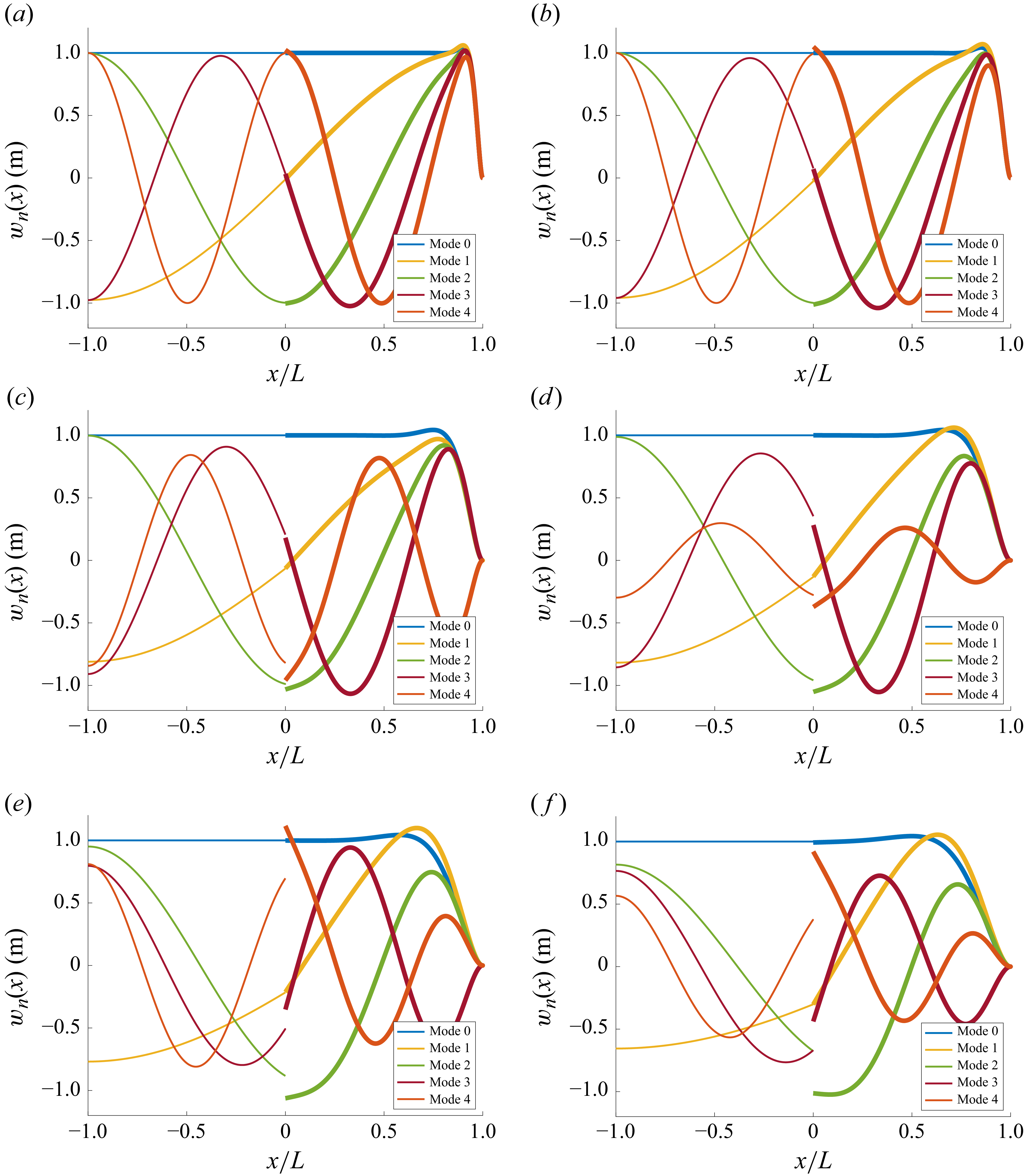
that solve this system determine the static bending shape of the ice shelf. Figure 2 shows the static mode (labelled Mode 0) for a range of ice shelf thicknesses, among other dynamic modes. The final check of our calculation is that this form matches the one found by the numerical limit and that it also gives a resolution of the identity, i.e. that we recover the initial condition with this mode.
$C_j$
that solve this system determine the static bending shape of the ice shelf. Figure 2 shows the static mode (labelled Mode 0) for a range of ice shelf thicknesses, among other dynamic modes. The final check of our calculation is that this form matches the one found by the numerical limit and that it also gives a resolution of the identity, i.e. that we recover the initial condition with this mode.
3.4. Orthogonality of the modes of vibration
Following Meylan (Reference Meylan2002) and Hazard & Meylan (Reference Hazard and Meylan2008), we define the inner product as
 \begin{align} \langle f_1, f_2 \rangle _{\mathcal{V}} = \rho _w g\! \int _{-L}^{L} f_1 \overline {f_2} \, \mathrm{d}x + D\! \int _0^L \frac {\partial ^2\! f_1}{\partial x^2} \frac {\partial ^2 \overline {f_2}}{\partial x^2} \, \mathrm{d}x, \end{align}
where $f_1$
and
$f_1$
and $f_2$
are arbitrary functions in the associated Hilbert space. The orthogonality of the eigenfunctions, namely
$f_2$
are arbitrary functions in the associated Hilbert space. The orthogonality of the eigenfunctions, namely
 \begin{align} \langle w_m, w_n \rangle _{\mathcal{V}} = 0 \quad \text{for} \quad \omega _m \ne \omega _n, \end{align}
plays a key role in enabling a valid modal decomposition of the solution. See Appendix A for the detailed proof of this fact.
4. Time-domain solution
The time evolution is governed by an abstract wave equation
 \begin{align} \partial _t^2 W + \mathcal{P} W=0, \end{align}
where $\mathcal{P}$
is the compact positive self-adjoint operator governing the transient dynamics of the ocean/ice shelf system. Without ice, we would simply have
$\mathcal{P}$
is the compact positive self-adjoint operator governing the transient dynamics of the ocean/ice shelf system. Without ice, we would simply have $\mathcal{P} = {-}\textit{gH} \partial _x^2$
, which yields the classical wave equation with wavespeed
$\mathcal{P} = {-}\textit{gH} \partial _x^2$
, which yields the classical wave equation with wavespeed $\sqrt {gH}$
. When the ice shelf is present, the form of
$\sqrt {gH}$
. When the ice shelf is present, the form of $\mathcal{P}$
is more complex, and we make no attempt to express it.
$\mathcal{P}$
is more complex, and we make no attempt to express it.
The eigenfunctions of $\mathcal{P}$
are those found in § 3, satisfying
$\mathcal{P}$
are those found in § 3, satisfying
 \begin{align} \mathcal{P} w_n = \omega _n^2 w_n. \end{align}
We assume the solution can be written as a modal expansion
 \begin{align} W(x,t) = \sum _{n=0}^\infty a_n(t)\, w_n(x), \end{align}
which, upon substitution into (4.1) and an application of orthogonality of $\{w_n\}$
, leads to
$\{w_n\}$
, leads to
 \begin{align} a_n''(t) = -\omega _n^2\, a_n(t). \end{align}
For $n\gt 0$
, this ordinary differential equation has solutions
$n\gt 0$
, this ordinary differential equation has solutions
 \begin{align} a_n(t) = C_n \cos (\omega _n t) + D_n\frac {\sin (\omega _n t)}{\omega _n} , \end{align}
where $C_n$
and
$C_n$
and $D_n$
are as-yet unknown coefficients. In the case
$D_n$
are as-yet unknown coefficients. In the case $n=0$
, (4.4) has solutions
$n=0$
, (4.4) has solutions
 \begin{align} a_0(t)=C_0+D_0t. \end{align}
Thus
 \begin{align} W(x,t) = (C_0+D_0t)\, w_0(x) + \sum _{n=1}^\infty \left [ C_n \cos (\omega _n t) + D_n\frac {\sin (\omega _n t)}{\omega _n} \right ] w_n(x). \end{align}
We perform simulations using all $N_{\textit{modes}}$
modes whose angular frequencies lie in the interval
$N_{\textit{modes}}$
modes whose angular frequencies lie in the interval $[0,1]$
s
$[0,1]$
s $^{-1}$
. The modal approximation, obtained from the truncated series representation, is given by
$^{-1}$
. The modal approximation, obtained from the truncated series representation, is given by
 \begin{align} W(x,t) = (C_0+D_0t)\,w_0(x) + \sum _{n=1}^{N_{\textit{modes}}} \left [ C_n \cos (\omega _n t) + D_n\frac {\sin (\omega _n t)}{\omega _n} \right ] w_n(x). \end{align}
The coefficients $C_n$
and
$C_n$
and $D_n$
are determined by the initial conditions. Since we have
$D_n$
are determined by the initial conditions. Since we have
 \begin{align} f(x) &= W(x,0) = \sum _{n=0}^\infty C_n w_n(x), \end{align}
 \begin{align} g(x) &= \partial _t\! W(x,0) = \sum _{n=0}^\infty D_n w_n(x), \end{align}
an application of orthonormality yields
 \begin{align} \langle f, w_n \rangle _{\mathcal{V}} = \int _0^L f(x) w_n(x) \, \mathrm{d}x, \end{align}
 \begin{align} \langle g, w_n \rangle _{\mathcal{V}} = \int _0^L g(x) w_n(x) \, \mathrm{d}x, \end{align}
since the eigenfunctions $w_n(x)$
have been normalised in the previous section, and the modal coefficients are
$w_n(x)$
have been normalised in the previous section, and the modal coefficients are
 \begin{align} C_n &= \langle f, w_n \rangle _{\mathcal V}, \end{align}
 \begin{align} D_n &= \langle g, w_n \rangle _{\mathcal V}. \end{align}
We evaluate these inner products numerically using midpoint quadrature. Suppose that the domain $(-L,L)$
is partitioned into
$(-L,L)$
is partitioned into $N$
subintervals
$N$
subintervals $(x_i-\Delta x/2,x_i+\Delta x/2)$
, where
$(x_i-\Delta x/2,x_i+\Delta x/2)$
, where $N$
is an even integer,
$N$
is an even integer, $x_i$
is the midpoint of the
$x_i$
is the midpoint of the $i$
th interval, and
$i$
th interval, and $\Delta x$
is the uniform spacing of the partition. Then we can approximate the coefficients
$\Delta x$
is the uniform spacing of the partition. Then we can approximate the coefficients $C_n$
and
$C_n$
and $D_n$
as
$D_n$
as
 \begin{align} C_n &\approx \rho _w g \sum _{i=1}^N f(x_i)\, w_n(x_i) \Delta x + D \sum _{i = ({N+1})/{2}}^N f(x_i)\, \frac {\partial ^4 w_n(x_i)}{\partial x^4} \, \Delta x, \end{align}
 \begin{align} D_n &\approx \rho _w g \sum _{i=1}^N g(x_i)\, w_n(x_i) \Delta x + D \sum _{i = ({N+1})/{2}}^N g(x_i)\, \frac {\partial ^4 w_n(x_i)}{\partial x^4} \, \Delta x. \end{align}
5. Results
In this section, we present numerical results of the proposed time-domain model of a bounded ice shelf subjected to various forcing scenarios. The results are divided into two parts. First, we analyse the natural mode shapes of the ice shelf for different thickness values. Second, we investigate the transient wave–ice shelf interaction using fixed thicknesses $50$
m and
$50$
m and $150$
m, and fixed ice shelf length
$150$
m, and fixed ice shelf length $L=10^4\ \text{m}$
. Error plots are included to demonstrate convergence with respect to the number of modes.
$L=10^4\ \text{m}$
. Error plots are included to demonstrate convergence with respect to the number of modes.
5.1. Natural mode shapes
Figure 2 shows the first five mode shapes for ice shelves with thicknesses ranging from $30$
m to
$30$
m to $250$
m. As the thickness increases, the mode shapes exhibit shorter wavelengths, reflecting the higher stiffness of the thicker shelves. For
$250$
m. As the thickness increases, the mode shapes exhibit shorter wavelengths, reflecting the higher stiffness of the thicker shelves. For $h = 150$
m and above, the mode shapes become increasingly influenced by the boundary conditions, with deformation concentrated closer to the edges, and reduced variation in the interior. An important feature visible in all modes is the discontinuity in slope at
$h = 150$
m and above, the mode shapes become increasingly influenced by the boundary conditions, with deformation concentrated closer to the edges, and reduced variation in the interior. An important feature visible in all modes is the discontinuity in slope at $x = 0$
. This is a physical consequence of the boundary and matching conditions imposed at the interface between the open water and the ice shelf. The change in flexural rigidity across this interface results in a discontinuity in the second derivative of displacement, consistent with the balance of bending moments and shear forces. The mode shapes have been scaled to have amplitudes ranging approximately between
$x = 0$
. This is a physical consequence of the boundary and matching conditions imposed at the interface between the open water and the ice shelf. The change in flexural rigidity across this interface results in a discontinuity in the second derivative of displacement, consistent with the balance of bending moments and shear forces. The mode shapes have been scaled to have amplitudes ranging approximately between $-1$
and
$-1$
and $1$
. This demonstrates how greater thickness shifts the dynamic response towards higher-frequency modes and boundary-dominated patterns, while also highlighting the localised mechanical response at the ice front.
$1$
. This demonstrates how greater thickness shifts the dynamic response towards higher-frequency modes and boundary-dominated patterns, while also highlighting the localised mechanical response at the ice front.
First five mode shapes for ice shelves with varying thicknesses. The modes have been rescaled to take values between $-1$
and
$-1$
and $1$
for clarity. The thicknesses are (a)
$1$
for clarity. The thicknesses are (a) $h = 30$
m, (b)
$h = 30$
m, (b) $h = 50$
m, (c)
$h = 50$
m, (c) $h = 100$
m, (d)
$h = 100$
m, (d) $h = 150$
m, (e)
$h = 150$
m, (e) $h = 200$
m, ( f)
$h = 200$
m, ( f) $h = 250$
m.
$h = 250$
m.

5.2. Time-domain solutions
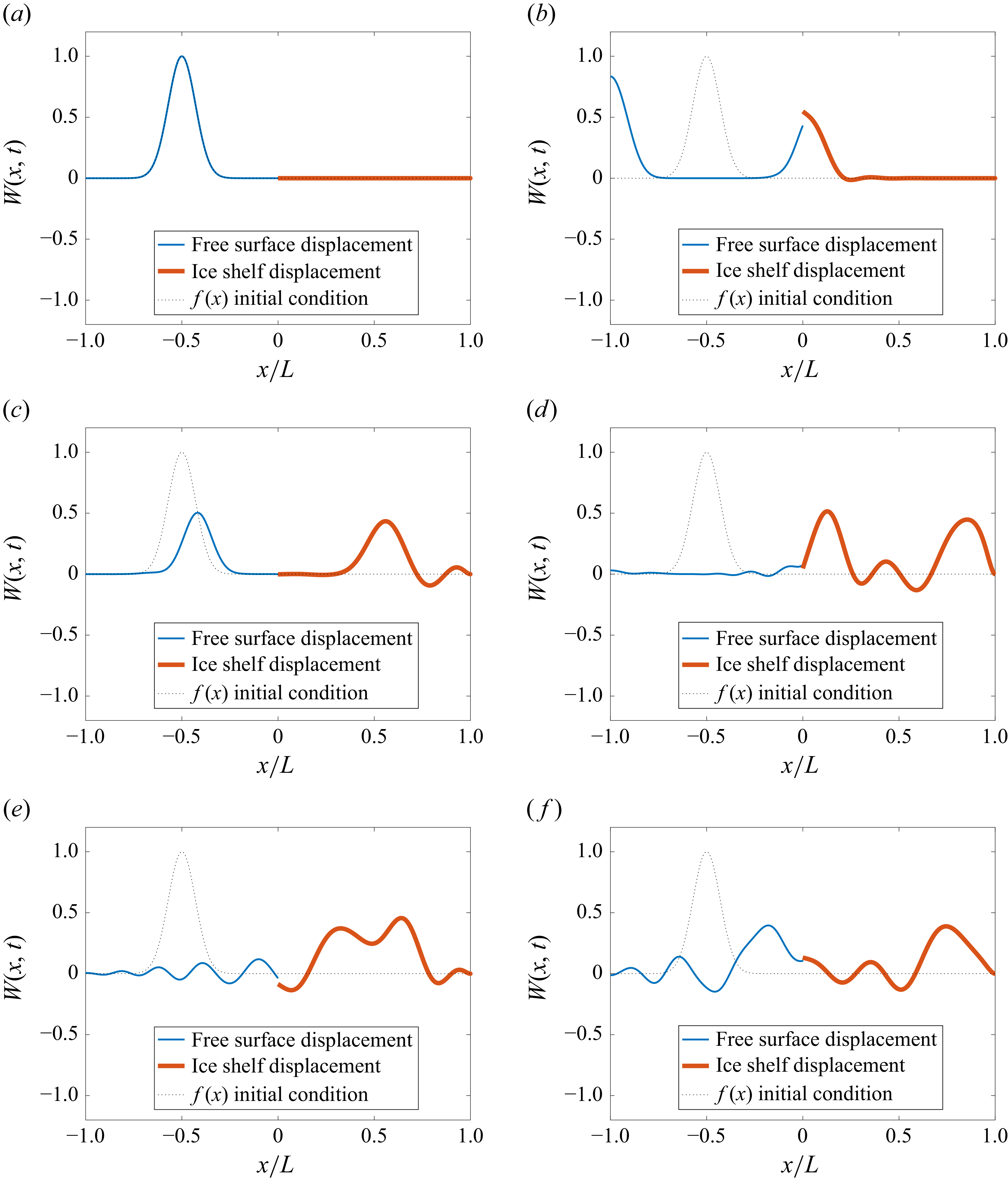
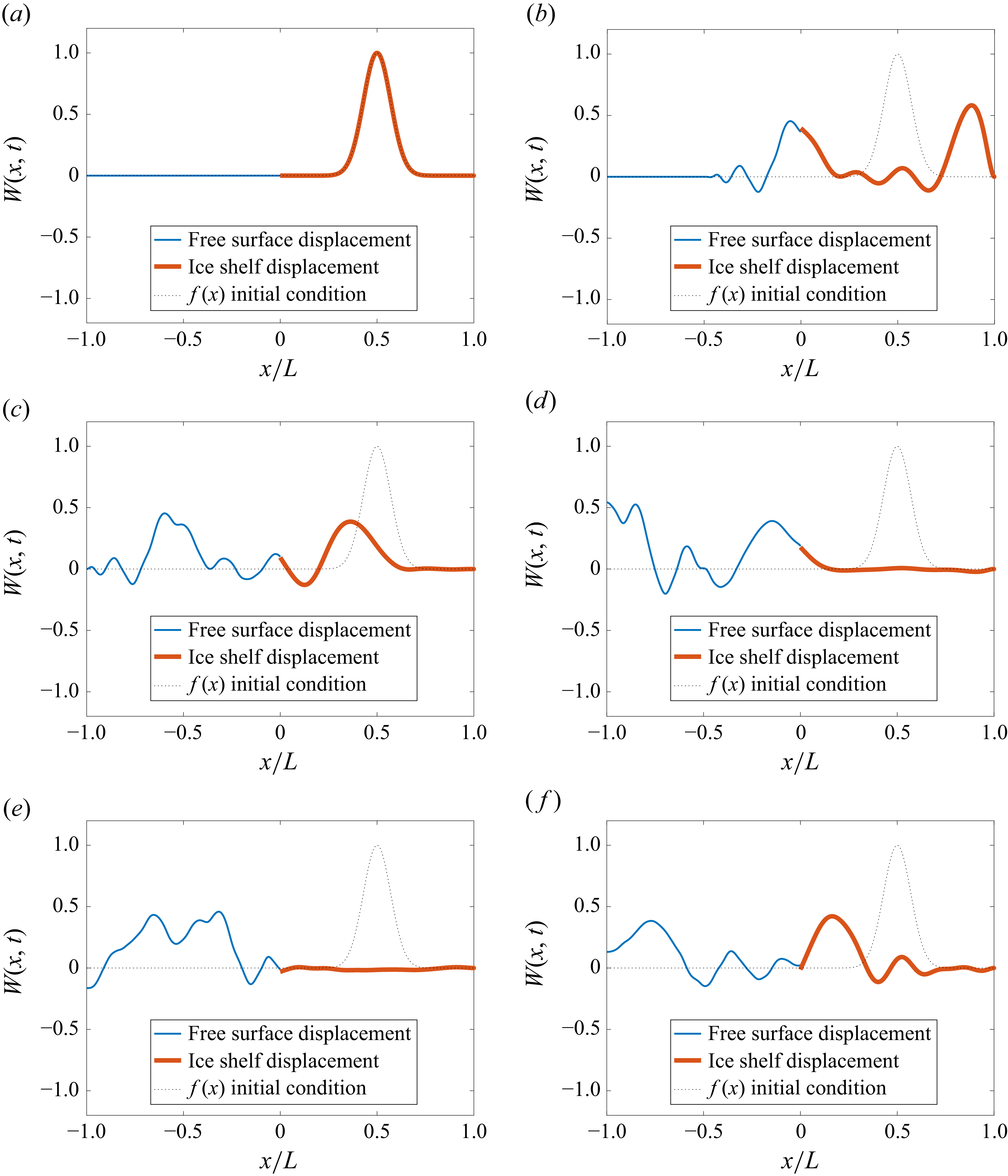
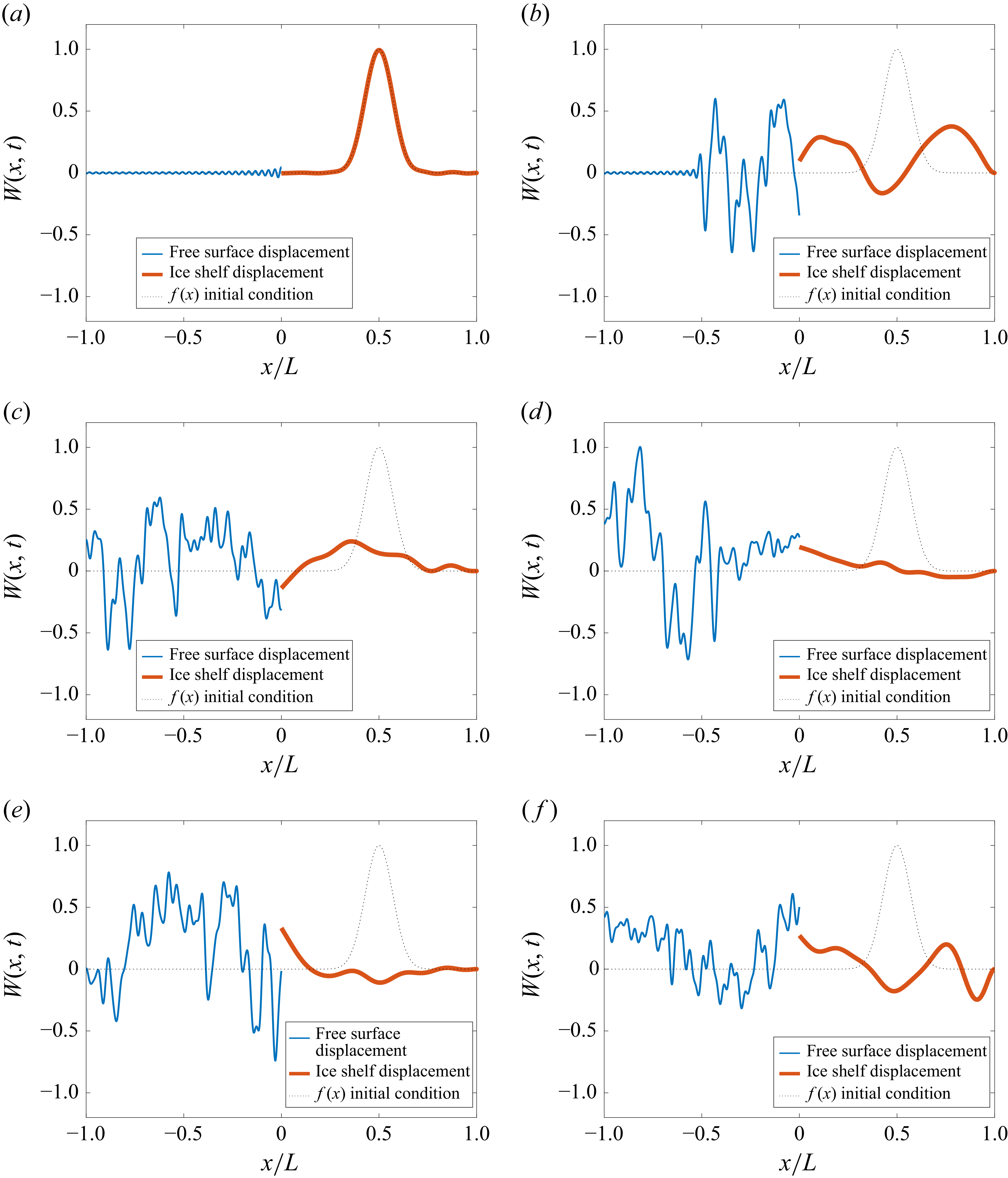
Figures 3, 4, 5 and 6 illustrate the time evolution of wave–ice shelf interaction for two ice shelf thicknesses: $h = 50$
m and
$h = 50$
m and $h = 150$
m. We consider two distinct initial conditions for each thickness. As shown in figure 6, it is difficult to approximate the initial condition, as higher-frequency modes are required to achieve the degree of bending imposed on the ice. This is evident in figure 6(
a), where the line is not perfectly flat for
$h = 150$
m. We consider two distinct initial conditions for each thickness. As shown in figure 6, it is difficult to approximate the initial condition, as higher-frequency modes are required to achieve the degree of bending imposed on the ice. This is evident in figure 6(
a), where the line is not perfectly flat for $x \lt 0$
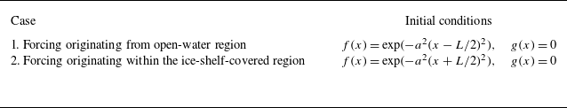
due to the insufficient representation of these high-frequency components. This could be resolved by including more modes. To investigate the transient response of the ice shelf system, we consider two different initial conditions, summarised in table 1. In both cases, the ice shelf is already deformed at
$x \lt 0$
due to the insufficient representation of these high-frequency components. This could be resolved by including more modes. To investigate the transient response of the ice shelf system, we consider two different initial conditions, summarised in table 1. In both cases, the ice shelf is already deformed at $ t = 0$
s due to the presence of a Gaussian wave packet.
$ t = 0$
s due to the presence of a Gaussian wave packet.
Time evolution of wave–ice shelf interaction (wave coming from water) for $h =50$
m: (a)
$h =50$
m: (a) $t = 0$
s, (b)
$t = 0$
s, (b) $t = 100$
s, (c)
$t = 100$
s, (c) $t = 200$
s, (d)
$t = 200$
s, (d) $t = 300$
s, (e)
$t = 300$
s, (e) $t = 400$
s, ( f)
$t = 400$
s, ( f) $t = 500$
s.
$t = 500$
s.

Time evolution of wave–ice shelf interaction (wave coming from water) for $h =150$
m: (a)
$h =150$
m: (a) $t = 0$
s, (b)
$t = 0$
s, (b) $t = 100$
s, (c)
$t = 100$
s, (c) $t = 200$
s, (d)
$t = 200$
s, (d) $t = 300$
s, (e)
$t = 300$
s, (e) $t = 400$
s, ( f)
$t = 400$
s, ( f) $t = 500$
s.
$t = 500$
s.

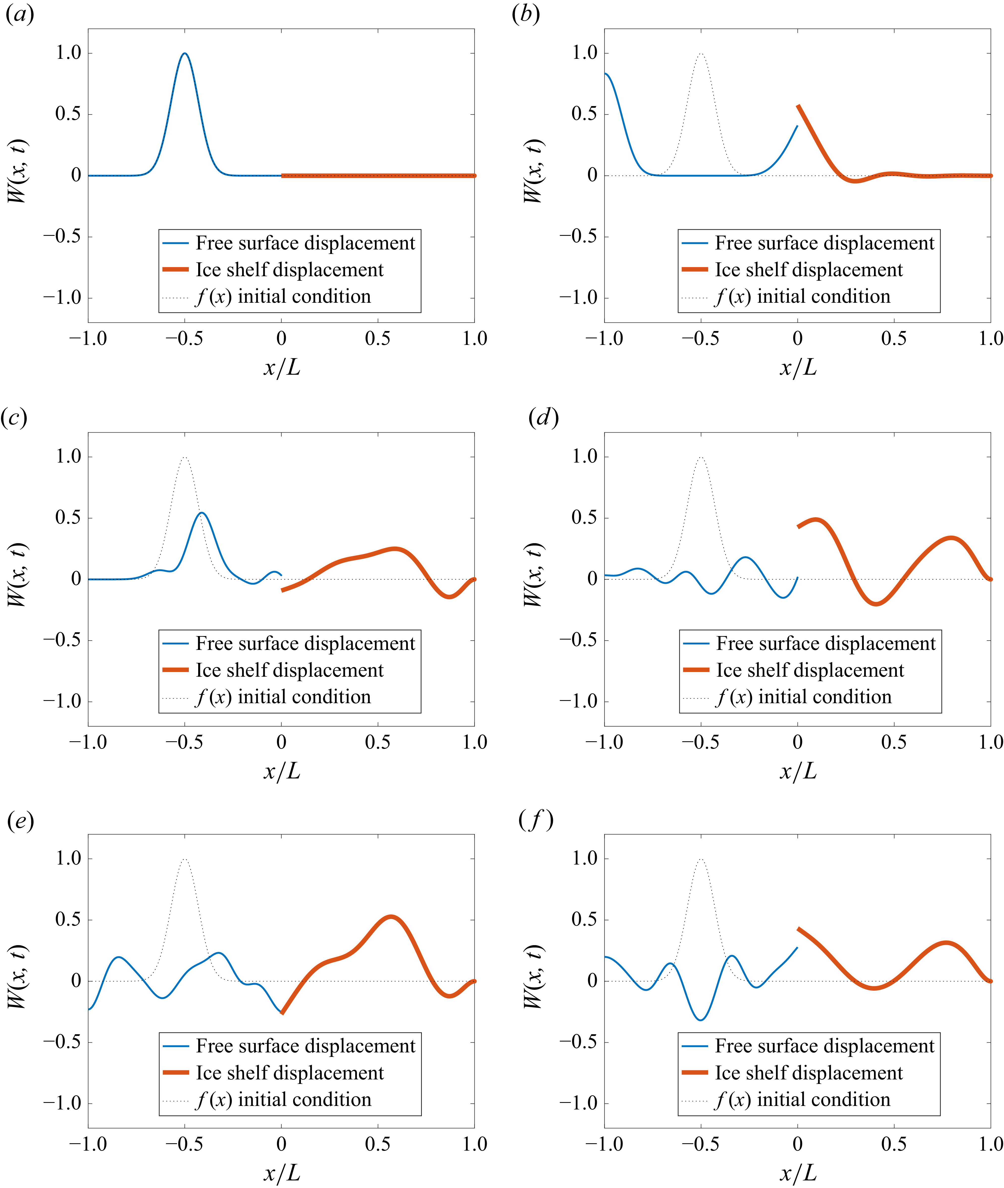
Time evolution of wave–ice shelf interaction (forcing originating from the ice-covered region) for $h =50$
m: (a)
$h =50$
m: (a) $t = 0$
s, (b)
$t = 0$
s, (b) $t = 100$
s, (c)
$t = 100$
s, (c) $t = 200$
s, (d)
$t = 200$
s, (d) $t = 300$
s, (e)
$t = 300$
s, (e) $t = 400$
s, ( f)
$t = 400$
s, ( f) $t = 500$
s.
$t = 500$
s.

Time evolution of wave–ice shelf interaction (forcing originating from the ice-covered region) for $h=150$
m: (a)
$h=150$
m: (a) $t = 0$
s, (b)
$t = 0$
s, (b) $t = 100$
s, (c)
$t = 100$
s, (c) $t = 200$
s, (d)
$t = 200$
s, (d) $t = 300$
s, (e)
$t = 300$
s, (e) $t = 400$
s, ( f)
$t = 400$
s, ( f) $t = 500$
s.
$t = 500$
s.

In both the thin and thick ice shelf configurations, the initial wave packet propagates to the left and right from its source location. The right-propagating component enters the ice shelf from the water side, exciting flexural vibrations upon transmission. The left-propagating component reflects off the left-hand boundary and subsequently travels back towards the ice shelf. As time advances ( $ t = 100$
, 200, 300, 400, 500 s), wave energy disperses within the ice domain, activating multiple vibration modes. These modes interact through reflection and interference, giving rise to complex transient responses and the formation of standing wave patterns.
$ t = 100$
, 200, 300, 400, 500 s), wave energy disperses within the ice domain, activating multiple vibration modes. These modes interact through reflection and interference, giving rise to complex transient responses and the formation of standing wave patterns.
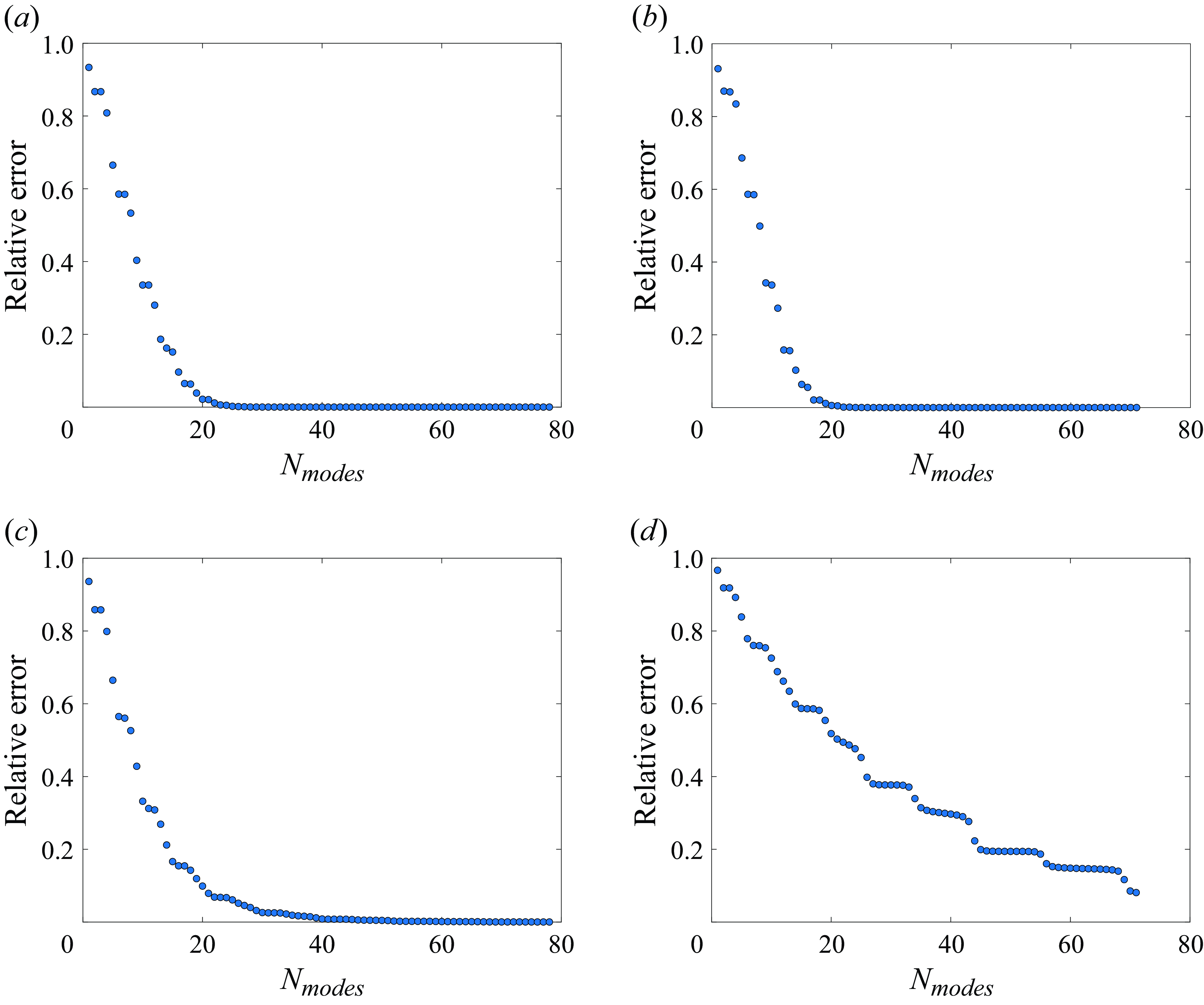
We assess the convergence of the modal expansion by computing the relative truncation error between the initial vertical displacement $f(x)$
and its modal approximation
$f(x)$
and its modal approximation $f_{N_{\textit{modes}}}(x)$
obtained using the first
$f_{N_{\textit{modes}}}(x)$
obtained using the first $N_{\textit{modes}}$
. The truncated representation is defined as
$N_{\textit{modes}}$
. The truncated representation is defined as
 \begin{align} f_{N_{\textit{modes}}}(x) = \sum _{n=0}^{N_{\textit{modes}}} C_n\, w_n(x). \end{align}
The relative error is expressed as
 \begin{align} \text{relative error}(N_{\textit{modes}}) = \frac {\| f - f_{N_{\textit{modes}}} \|}{\| f \|}, \end{align}
where $\|{\cdot }\|$
denotes the canonical norm associated with the energy inner product (3.13). Figure 7 illustrates the decay of the relative error with increasing mode number
$\|{\cdot }\|$
denotes the canonical norm associated with the energy inner product (3.13). Figure 7 illustrates the decay of the relative error with increasing mode number $N_{\textit{modes}}$
. With a water-incident wave at
$N_{\textit{modes}}$
. With a water-incident wave at $h = 50\ \text{m}$
and
$h = 50\ \text{m}$
and $h = 150\ \text{m}$
, figures 7(a,b) show rapid convergence, with relative error less than
$h = 150\ \text{m}$
, figures 7(a,b) show rapid convergence, with relative error less than $2\times 10^{-4}$
for
$2\times 10^{-4}$
for $N_{\textit{modes}}\gt 29$
. In the case where the ice is initially bent, convergence at
$N_{\textit{modes}}\gt 29$
. In the case where the ice is initially bent, convergence at $h = 50\ \text{m}$
(figure 7
c) is slightly slower than when the fluid is initially displaced, with relative error under
$h = 50\ \text{m}$
(figure 7
c) is slightly slower than when the fluid is initially displaced, with relative error under $3.18\times 10^{-2}$
for
$3.18\times 10^{-2}$
for $N_{\textit{modes}}\gt 29$
. Moreover, when
$N_{\textit{modes}}\gt 29$
. Moreover, when $h = 150\,m$
(figure 7
d), convergence for the initial ice deformation problem is slow, with relative error
$h = 150\,m$
(figure 7
d), convergence for the initial ice deformation problem is slow, with relative error $8.11\times 10^{-2}$
for mode number
$8.11\times 10^{-2}$
for mode number $71$
. This poor convergence, which is visible as erroneous oscillations in figure 6(
a), is due to the fact that many high-frequency modes are excited when the thicker ice is bent in that way. Although we could have obtained a more accurate solution by increasing
$71$
. This poor convergence, which is visible as erroneous oscillations in figure 6(
a), is due to the fact that many high-frequency modes are excited when the thicker ice is bent in that way. Although we could have obtained a more accurate solution by increasing $N_{\textit{modes}}$
, we have included the less accurate solution here to illustrate the limitation of our method for thick ice.
$N_{\textit{modes}}$
, we have included the less accurate solution here to illustrate the limitation of our method for thick ice.
Initial displacement profiles for the two considered cases. In each case, the initial condition is given by a pair $(f(x), g(x))$
, where
$(f(x), g(x))$
, where $f(x)$
denotes the initial displacement, and
$f(x)$
denotes the initial displacement, and $g(x)$
denotes the initial velocity. The parameter
$g(x)$
denotes the initial velocity. The parameter $ a = 10^{-3}\ \mathrm{m}^{-1}$
controls the localisation of the profile.
$ a = 10^{-3}\ \mathrm{m}^{-1}$
controls the localisation of the profile.

Relative error of the modal approximation for ice shelves with thicknesses (a,c) $h = 50$
m and (b,d)
$h = 50$
m and (b,d) $h = 150$
m. (a,b) Corresponding results for waves incident from the water side. (c,d) Error behaviour for the forcing originating from the ice-covered region.
$h = 150$
m. (a,b) Corresponding results for waves incident from the water side. (c,d) Error behaviour for the forcing originating from the ice-covered region.

6. Summary
In this work, we developed a mathematical model of a bounded ice shelf coupled to the ocean, combining Kirchhoff–Love plate theory for the ice shelf with linear shallow-water wave theory for the fluid. Matching conditions were applied at the ice–water interface to ensure continuity of the velocity potential, and boundary conditions were imposed at the edges of both the ice shelf and the fluid domain. The resulting nonlinear matrix eigenvalue problem was solved numerically to obtain the natural modes and frequencies of vibration of the coupled system, which form the basis for constructing time-domain solutions via a spectral method. The time-domain simulations illustrated how transient wave packets interact with the ice shelf structure, exciting multiple modes and generating complex interference patterns through boundary reflections. These examples serve primarily to demonstrate the capabilities of the modelling framework and solution method.
The primary aim of this study was to establish a framework for solving initial value problems for a domain with partial ice shelf cover. We note that the model is highly simplified, and consideration of variable thickness, water depth, three-dimensional effects, variation in ice shelf properties with depth, and so on, needs to be incorporated to make qualitative predictions for particular ice shelves. However, any model incorporating such effects would have to include the model presented here as a particular case. Thus this work enables an extension to simulating the sequential break-up of ice shelves, a proposed model of ice shelf break-up in which wave-induced mechanical stresses cause instantaneous fracture events, resulting in disintegration over time. By extending the model to incorporate nonlinear effects (especially break-up), wave scattering, and interaction with floating sea ice or open water, further insights into ice shelf stability and retreat may be achieved. In addition, extending the model to an infinite domain would represent a major change, as it leads to a continuous spectrum of modes and requires a different theoretical framework. A possible improvement of the model is to extend it for very thick ice shelves, where additional wave modes may appear. Another direction is to use a Mindlin plate formulation to capture these effects with more precision.
Supplementary movies
Supplementary movies are available at https://doi.org/10.1017/jfm.2025.11050.
Funding
This study is supported via funding to F.A. from Prince sattam bin Abdulaziz University project number PSAU/2025/R/1447. M.H.M. and B.W. are supported by the Australian Research Council’s Discovery Projects funding scheme (DP240102104).
Declaration of interests
The authors report no conflict of interest.
Data availability statement
The data that support the findings of this study are openly available in Time-Domain-Analysis-of-an-Ice-Shelf-in-a-Bounded-Domain-Code at http://doi.org/10.5281/zenodo.18081870. See JFM’s research transparency policy for more information.
Author contributions
Conceptualisation: F.A., M.H.M. and B.W. Methodology: F.A., M.H.M. and B.W. Software: F.A. Validation: F.A. Writing – original draft preparation: F.A. Writing – review and editing: M.H.M. and B.W. Visualisation: F.A. Supervision: M.H.M. and B.W. All authors have read and agreed to the published version of the paper.
Appendix A. Proof of modes orthogonality
We aim to demonstrate the orthogonality relation (3.14). This orthogonality ensures the independence of modal contributions, and enables a valid modal decomposition of the solution. Note that this orthogonality is closely related to the derivation in Hazard & Meylan (Reference Hazard and Meylan2008), with the exception that in that work, the fluid was of finite depth and the domain was infinite. The derivation in Meylan (Reference Meylan2002) was for shallow water, but it assumed that the inertia term of the plate was negligible. In order to show (3.14), we will show the stronger condition that
 \begin{align} \omega _m^2\langle w_m, w_n \rangle _{\mathcal{V}}=\omega _n^2\langle w_m, w_n \rangle _{\mathcal{V}}, \end{align}
which also implicitly shows that the underlying operator is self-adjoint and positive since the eigenvalue is $\omega _n^2$
. To proceed, we split the integration from
$\omega _n^2$
. To proceed, we split the integration from $ -L$
to
$ -L$
to $ L$
into two parts:
$ L$
into two parts:
 \begin{align} \omega _m^2\langle w_m, w_n \rangle _{\mathcal{V}}&=\omega _m^2\! \left ( \rho _w g\! \int _{-L}^{L} w_m \overline {w_n} \, \mathrm{d}x + D\! \int _{0}^{L} \frac {\partial ^2 w_m}{\partial x^2} \frac {\partial ^2 \overline {w_n}}{\partial x^2} \, \mathrm{d}x \right ) \nonumber \\ &=\rho _w g \omega _m^2\! \int _{-L}^{0} w_m \overline {w_n} \, \mathrm{d}x + \rho _w g \omega _m^2\! \int _{0}^{L} w_m \overline {w_n} \,\mathrm{d} x\nonumber \\ &\quad + \omega _m^2 D\! \int _{0}^{L} \frac {\partial ^2 w_m}{\partial x^2} \frac {\partial ^2 \overline {w_n}}{\partial x^2} \,\mathrm{d} x. \end{align}
We integrate by parts twice for the region under the ice to transfer the derivative from $w_m$
to
$w_m$
to $ \overline {w_n}$
:
$ \overline {w_n}$
:
 \begin{align} \omega _m^2\langle w_m, w_n \rangle _{\mathcal{V}}&= \rho _w g \omega _m^2 \int _{-L}^{0} w_m \overline {w_n} \, \mathrm{d}x + \rho _w g \omega _m^2 \int _{0}^{L} w_m \overline {w_n} \, \mathrm{d}x\nonumber \\&\quad + \omega _m^2 D \left ( \left [ \frac {\partial w_m}{\partial x} \frac {\partial ^2 \overline {w_n}}{\partial x^2} \right ]_{0}^{L} - \left [ w_m \frac {\partial ^3 \overline {w_n}}{\partial x^3} \right ]_{0}^{L} + \int _{0}^{L} \frac {\partial ^4 \overline {w_n}}{\partial x^4} w_m \, \mathrm{d}x \right )\!. \end{align}
We combine and simplify the integrals from $ 0$
to
$ 0$
to $ L$
:
$ L$
:
 \begin{align} \omega _m^2\langle w_m, w_n \rangle _{\mathcal{V}}= \rho _w g \omega _m^2 \int _{-L}^{0} w_m \overline {w_n} \, \mathrm{d}x + \omega _m^2 \int _{0}^{L} w_m\left ( \rho _w g \overline {w_n}+D \frac {\partial ^4 \overline {w_n}}{\partial x^4} \right ) \mathrm{d}x. \end{align}
We substitute (2.5a
) in the region from $ 0$
to
$ 0$
to $ L$
, and substitute (2.5b
) and (2.5c
) in the open-water region. After performing integration by parts twice, we obtain
$ L$
, and substitute (2.5b
) and (2.5c
) in the open-water region. After performing integration by parts twice, we obtain
 \begin{align} \omega _m^2\langle w_m, w_n \rangle _{\mathcal{V}}&= - \rho _w \omega _n \omega _m H \Bigg ( \big [ \partial _x \phi _m \, \overline {\phi _n} \big ]_{-L}^{0} - \big [ \phi _m \, \partial _x \overline {\phi _n} \big ]_{-L}^{0} + \int _{-L}^{0} \phi _m \, \partial _x^2 \overline {\phi _n} \, \mathrm{d}x \Bigg ) \nonumber \\ &\quad {}+ \omega _m^2 \int _{0}^{L} w_m\big ( \omega _n^2 \rho _I h \overline {w_n} - \mathrm{i} \omega _n \rho _w \overline {\phi _n}\big ) \, \mathrm{d}x. \end{align}
We substitute (2.5b ) and (2.5c ) back into the integration and simplify, yielding
 \begin{align} \begin{split} \omega _m^2\langle w_m, w_n \rangle _{\mathcal{V}}&= \omega _n^2 \rho _w g\! \int _{-L}^{0} w_m \overline {w_n} \, \mathrm{d}x + \int _{0}^{L} \omega _n^2 \big ( \omega _m^2 \rho _I h w_m \big ) \overline {w_n} \, \mathrm{d}x \\ &\quad {}+ \int _{0}^{L} \omega _m^2 w_m \big ( -\mathrm{i} \omega _n \rho _w \overline {\phi _n} \big ) \, \mathrm{d}x. \end{split} \end{align}
We substitute (2.5a
) back into the integral from $ 0$
to
$ 0$
to $ L$
and simplify, yielding
$ L$
and simplify, yielding
 \begin{align} \omega _m^2\langle w_m, w_n \rangle _{\mathcal{V}}&= \omega _n^2 \rho _w g \int _{-L}^{0} w_m \overline {w_n} \, \mathrm{d}x + \int _{0}^{L} \omega _n^2 \left (D \frac {\partial ^4 w_m}{\partial x^4}\right ) \overline {w_n} \, \mathrm{d}x \nonumber \\ &\quad {}+ \omega _n^2 \rho _w g \int _{0}^{L} w_m \overline {w_n} \, \mathrm{d}x - \int _{0}^{L} \omega _n^2 \big (\mathrm{i} \omega _m \rho _w \phi _m \big ) \overline {w_n} \, \mathrm{d}x \nonumber \\ &\quad {}+ \int _{0}^{L} \omega _m^2 w_m \big ( -\mathrm{i} \omega _n \rho _w \overline {\phi _n} \big ) \, \mathrm{d}x. \end{align}
By integrating the fourth derivative term by parts twice, applying the boundary conditions, and combining the integrals, we get
 \begin{align} \omega _m^2\langle w_m, w_n \rangle _{\mathcal{V}}&= \rho _w g\! \int _{-L}^{L} \omega _n^2 w_m \overline {w_n} \, \mathrm{d}x + \omega _n^2 D\! \int _{0}^{L} \frac {\partial ^2 w_m}{\partial x^2} \, \frac {\partial ^2 \overline {w_n}}{\partial x^2} \, \mathrm{d}x \nonumber \\ &\quad {}+ \int _{0}^{L} \omega _m^2 w_m \big ( -\mathrm{i} \rho _w \omega _n \overline {\phi _n} \big ) \, \mathrm{d}x + \int _{0}^{L} \big ({-}\mathrm{i} \omega _m \rho _w \phi _m \big ) \omega _n^2 \overline {w_n} \, \mathrm{d}x. \end{align}
Finally, we substitute (2.5c ), and integrate one of the terms by parts twice, applying the boundary conditions, which yields the desired result:
 \begin{align} \begin{split} \omega _m^2\langle w_m, w_n \rangle _{\mathcal{V}}&= \omega _n^2\! \left ( \rho _w g \int _{-L}^{L} w_m \overline {w_n} \, \mathrm{d}x + D \int _{0}^{L} \frac {\partial ^2 w_m}{\partial x^2} \frac {\partial ^2 \overline {w_n}}{\partial x^2} \, \mathrm{d}x \right )\!. \end{split} \end{align}


 Open access