







1. Introduction
The breaking of surface ocean gravity waves is a highly dissipative process at the air–sea interface that affects the evolution of the ocean wave field, as well as the dynamics of the upper ocean and the lower atmosphere. Wave breaking enhances the exchange of mass, momentum, gases and heat across the air–sea interface, balances the energy input from the wind to the wave field and limits the height of individual waves (Melville Reference Melville1996; Wanninkhof et al. Reference Wanninkhof, Asher, Ho, Sweeney and McGillis2009; Latheef & Swan Reference Latheef and Swan2013; Perlin, Choi & Tian Reference Perlin, Choi and Tian2013; Veron Reference Veron2015). The magnitude of these interfacial processes is in large part determined by the severity of, or the amount of energy dissipated by, individual breaking waves.
Breaking waves occur naturally in sufficiently steep irregular wave fields where a large number of fundamental frequency components coexist and interact nonlinearly. While breaking waves themselves are typically discrete isolated events occurring at the crest of an individual wave, they can form as a result of the interaction of a range of frequency components within a wave group. It would be reasonable to expect then, that the characteristics of the breaking process in terms of breaking onset, energy loss and two-phase flow properties, should be influenced by the underlying spectral properties of the wave group within which the breaking wave occurs.
One such spectral property is the bandwidth which describes how the energy of the underlying wave group is spread across different frequencies within the wave group (Saulnier et al. Reference Saulnier, Clément, Falcão, Pontes, Prevosto and Ricci2011). In broad qualitative terms, wave spectra may be described as either narrowband or broadband. This is shown graphically in figure 1 where panel (a) shows four different JONSWAP-type wave spectra (described in detail in § 2.2) of equal underlying energy, but different peak enhancement factors,  $\gamma$. The $\gamma$ value is not an explicit measure of bandwidth, but different values fundamentally alter the bandwidth of the corresponding wave spectra (Tian, Perlin & Choi Reference Tian, Perlin and Choi2012), by changing the spectral energy distribution. To be explicit, as clearly seen in figure 1(a), the smaller the value of $\gamma$ the more broadband the wave spectra are. This $\gamma$–bandwidth relationship is further illustrated in figure 1(b) which shows that different $\gamma$ values result in different wave steepness spectra. While the term bandwidth intuitively relates to the distribution of energy within a wave spectrum, we note that actual definitions of bandwidth vary considerably which can lead to difficulties comparing and contrasting results across studies. Appendix A discusses a variety of bandwidth definitions found in the literature and details their relationship to wave steepness and $\gamma$ values. In what follows, we use changes in the peak enhancement factor, $\gamma$, to change the underlying bandwidth of the wave groups studied here.
(a) Plots of the JONSWAP-type variance density spectra,  $S_{\eta \eta }(\,f_{i}) = 0.5 a_{i}^2 / \delta f$, used in the present study normalised by the maximum value of the most narrowband spectrum, $S_{\eta \eta }(\,f_{p})|_{\gamma =4}$. Here, $d$ is the water depth and $k_i$ and $a_i$ represent the wavenumber and amplitude of $i$th frequency component, $f_i$. We use $\delta f$ to denote the discretisation in the frequency domain and $f_p$ is the peak frequency. The bandwidth increases with decreasing peak enhancement factor, $\gamma$. The dashed red line represents tanh $(k_id)$ plotted against the right $y$-axis. (b) Plots of wave steepness distribution. Although these four spectra have the same linear amplitude sum, the equivalent values of linear steepness sum, $\sum a_i k_i$, are 0.29, 0.27, 0.26 and 0.25 from $\gamma =1$ to 4.

In the ocean, it is non-trivial to determine the directionally spread bandwidth of discrete wave groups in which individual waves break, and to then assess the role that bandwidth plays in the dynamics of those breaking waves. Due to this difficulty, dedicated laboratory studies are required to understand the specific role of bandwidth on the onset of breaking in wave groups as well as the fractional and absolute energy loss associated with those breaking waves. This paper describes a set of laboratory experiments conducted in intermediate to deep water to evaluate the role that bandwidth plays on the energetics and onset of breaking waves. It should be mentioned that the following review of previous studies focuses on deep and intermediate water waves.
There are very few studies that explicitly examine the role of bandwidth in breaking waves and the literature demonstrates that the role of bandwidth on breaking is not yet fully understood. Several studies argue that bandwidth plays an important role in the onset and energy dissipation of limiting and breaking waves (e.g. Wu & Yao Reference Wu and Yao2004; Drazen, Melville & Lenain Reference Drazen, Melville and Lenain2008; Tian, Perlin & Choi Reference Tian, Perlin and Choi2010; Liang et al. Reference Liang, Zhang, Sun and Chang2017; Alberello et al. Reference Alberello, Chabchoub, Monty, Nelli, Lee, Elsnab and Toffoli2018; Craciunescu & Christou Reference Craciunescu and Christou2020; Pizzo et al. Reference Pizzo, Murray, Smith and Lenain2021; Sinnis et al. Reference Sinnis, Grare, Lenain and Pizzo2021), but among these, there is disagreement on whether waves generated with relatively broadband wave spectra break at smaller (e.g. Wu & Yao Reference Wu and Yao2004; Liang et al. Reference Liang, Zhang, Sun and Chang2017; Alberello et al. Reference Alberello, Chabchoub, Monty, Nelli, Lee, Elsnab and Toffoli2018) or larger wave steepness (e.g. Drazen et al. Reference Drazen, Melville and Lenain2008; Pizzo et al. Reference Pizzo, Murray, Smith and Lenain2021; Sinnis et al. Reference Sinnis, Grare, Lenain and Pizzo2021). Nevertheless despite this apparent disagreement, Sinnis et al. (Reference Sinnis, Grare, Lenain and Pizzo2021) demonstrate that incorporating a measure of bandwidth successfully decreases the order of magnitude scatter in the relationship between the Duncan (Reference Duncan1981) breaking strength parameter,  $b$, and a modified measure of spectral wave steepness. In addition, Kway, Loh & Chan (Reference Kway, Loh and Chan1998) and Liang et al. (Reference Liang, Zhang, Sun and Chang2017) examined breaking wave energy dissipation using constant-amplitude spectra and Pierson–Moskowitz spectra and found that fractional energy loss is greater for breaking waves generated with constant-amplitude spectra. This suggests that how energy is distributed across the wave spectrum is important in determining the energy loss in breaking waves. Furthermore, Zhang & Yuan (Reference Zhang and Yuan2005) found that the distribution of spectral energy losses and gains in wave spectra as a result of wave breaking are dependent on the underlying wave spectrum used, again pointing to the potentially important role of spectral type and bandwidth. However, notwithstanding this body of evidence, some studies have argued that bandwidth effects in breaking wave energy dissipation, if present at all, are weak (Tian et al. Reference Tian, Perlin and Choi2010) and secondary to wave steepness (Rapp & Melville Reference Rapp and Melville1990; Perlin et al. Reference Perlin, Choi and Tian2013). It is worth pointing out that there is evidence that changes to wave spectra can lead to changes in some bandwidth measures, but not others (see table 1 in Wu & Yao Reference Wu and Yao2004), which also highlights the importance of understanding the precise definition of bandwidth used.
In this paper we report on the results from a laboratory study of breaking waves designed to quantify the influence of bandwidth on the evolution of spectral energy and wave group velocity, energy dissipation, energy dissipation rate and  $b$. This has been achieved by using an underlying wave spectrum with fixed frequency limits and constant peak frequency, which has been systematically altered in both amplitude and bandwidth. The remaining sections in the paper are structured as follows. Section 2 presents a description of the experimental set-up as well as breaking wave generation and conditions. Measures of characteristic wave parameters (wave steepness and bandwidth) and energy dissipation quantification are described in § 3. The influence of bandwidth on wave spectrum evolution, characteristic wave group velocity, wave energy dissipation and its rate and $b$ is provided in § 4. The main findings of the paper are listed in § 5. Lastly, in Appendix A, we provide various definitions of bandwidth and interpret their differences, and Appendix B quantifies the relationship between the different measures of wave steepness used here.
2. Experimental work
2.1. Experimental set-up
The experiments were conducted in the wind–wave flume at the Hydrodynamics Laboratory at Imperial College London. This flume is  $27$ m long, $0.3$ m wide with an operational water depth of $0.7$ m (see figure 2). At one end of the flume, a hinged-type wave paddle (paddle 1) was used to generate deep and intermediate water waves. At the opposite end, an identical wave paddle (paddle 2) actively absorbed the incident wave energy. In addition, a parabolic-shaped beach was placed in front of the paddle 2 to provide additional passive dissipation of incident wave energy. The combination of the active and passive solutions resulted in wave energy reflections of about $3\,\%$.
Schematic of the wind–wave flume. Key locations and instruments are highlighted.

A total number of 7 drop-down resistance-type wave gauges sampled at a frequency of 64 Hz were positioned along the centreline of the flume. The distances of the wave gauges to paddle 1 are shown in figure 2. The generation of wave groups (described in detail in § 2.2) was designed in such a way that individual waves broke between wave gauges 5 and 6. Within this region of interest, a 2.5 megapixel charge-coupled device (CCD) camera operating at 25 Hz was used to image the breaking process.
2.2. Wave-group generation
The breaking waves were generated using a dispersive focusing technique (Rapp & Melville Reference Rapp and Melville1990; Kway et al. Reference Kway, Loh and Chan1998; Drazen et al. Reference Drazen, Melville and Lenain2008; Tian et al. Reference Tian, Perlin and Choi2010, Reference Tian, Perlin and Choi2012; Callaghan, Deane & Stokes Reference Callaghan, Deane and Stokes2016; Liang et al. Reference Liang, Zhang, Sun and Chang2017; Zhang, Liang & Sun Reference Zhang, Liang and Sun2019). The surface elevation,  $\eta (x,t)$, is calculated by linear superposition of $N$ sinusoidal frequency components, each of a different frequency and amplitude, which can be given by
 \begin{equation} \eta(x, t) =\sum_{i=1}^{N} a_{i} \cos \left(k_{i} x-2 {\rm \pi}\,f_{i} t+\phi_{i}\right), \end{equation}
where  $a_{i}$, $k_{i}$, $f_{i}$ and $\phi _{i}$ represent the amplitude, wavenumber, frequency and phase of each underlying component $i$, respectively. Here $f_{i}$ were evenly distributed between $f_1$ and $f_N$, resulting in equal space between two adjacent components. By setting $\phi _{i} = -k_{i} x_{b} + 2{\rm \pi} f_{i} t_{b}$, linear wave theory is used to control the position and time of occurrence of the breaking waves. As the steepness and nonlinearity of the underlying wave group increases, the accuracy of linear theory breaks down and the desired $x_{b}$ was achieved by trial and error. In the present study, $t_b$ was set to 32 s.
JONSWAP spectra were used in the present study but were reformulated in the context of NewWave theory as it is believed to provide an accurate representation of large individual ocean waves (Tromans, Anatruk & Hagemeijer Reference Tromans, Anatruk and Hagemeijer1991). The JONSWAP spectrum of Hasselmann et al. (Reference Hasselmann1973) is defined by
 \begin{equation}
S_{\eta \eta}(\omega)=\frac{\chi g^{2}}{\omega^{5}} \exp
\left(\frac{-\beta \omega_{p}^{4}}{\omega^{4}}\right)
\gamma^{\exp ({-(\omega-\omega_{p})^{2}}/{2
\sigma^{2} \omega_{p}^{2}})},
\end{equation}
\begin{equation}
S_{\eta \eta}(\omega)=\frac{\chi g^{2}}{\omega^{5}} \exp
\left(\frac{-\beta \omega_{p}^{4}}{\omega^{4}}\right)
\gamma^{\exp ({-(\omega-\omega_{p})^{2}}/{2
\sigma^{2} \omega_{p}^{2}})},
\end{equation}
where  $\omega$ and $\omega _p$ refer to angular frequency and peak angular frequency, $\chi$ is the Phillips parameter equal to 0.0081, the shape coefficients $\beta$ and $\sigma$ have typical values of 1.25 and 0.07 if $\omega \le \omega _p$ and of 1.25 and 0.09 if $\omega > \omega _p$, respectively. As demonstrated in § 1, $\gamma$ is the peak enhancement factor representing how concentrated the spectral energy is around the peak frequency and, hence, the bandwidth. According to Tromans et al. (Reference Tromans, Anatruk and Hagemeijer1991), the discretised NewWave spectral amplitudes are related to the discretised JONSWAP spectral amplitudes, $a_{i,JONSWAP}$, following
 \begin{equation} a_i = \xi \, a^{2}_{i,JONSWAP}, \end{equation}
where  $a_{i,JONSWAP}=\sqrt {2 S_{\eta \eta }(\omega _i) \delta \omega }$ and $\xi$ is an appropriate scaling factor.
2.3. Wave conditions
The spectra used here had a fixed peak frequency of  $f_p=1/T_p$, where $T_p$ was the peak wave period of 1.2 s. The lower and upper frequency limits were 0.5 $f_p$ and 3 $f_p$, respectively. The resulting wave groups had a repeat time of 64 s (which gives a corresponding frequency discretisation of 1/64 Hz) and contained $N = 135$ individual spectral components. As previously shown in figure 1, the bandwidth of the underlying wave spectra was altered by modifying the peak enhancement factor, $\gamma$, from a minimum of 1 to a maximum of 4. For each $\gamma$, a sequence of wave groups with increasing linear amplitude sum, $A$ (
$A$ ( $=\sum _{i=1}^{N} a_{i}$), from non-breaking through incipient breaking to plunging was used, as summarised in table 1.
Experimental conditions:  $A$ is the linear amplitude sum measured at $x_5$ (the closest wave gauge to the focal location $x_b$).

Continually increasing  $A$ increases the nonlinearity of the underlying wave group and leads to the transition from non-breaking to breaking of the target focused wave (Baldock et al. Reference Baldock, Swan, Taylor and Smith1996). Further increases in $A$ can lead to the breaking of both the target focused wave and the preceding wave in the group, giving rise to multiple breaking waves within a single group. With yet further increases in $A$, a single breaking wave is recovered but breaking is confined to the wave in front of the target focused wave, which itself does not break. This pattern can continue as $A$ increases further, as has been described previously in Rapp & Melville (Reference Rapp and Melville1990). For the present study, only single breaking wave groups were considered.
The accurate generation of target spectra in the wave flume is demonstrated in figure 3, where panels (a–d) show the measured and target amplitude spectrum for wave groups with  $A = 20$ mm and $\gamma$ values of 1–4, respectively. The figures demonstrate excellent agreement between the measured and target spectra for all $\gamma$ values except at relatively high frequencies where the spectral energy is low. It is seen that at these frequencies the measured amplitude spectra begin to deviate from the target spectra, which is predominantly due to second-order wave–wave interactions that are not captured by linear theory. The inset figures in each panel show the measured and target phasing of the individual spectral components. For a perfectly focused wave, all phase components would lie on the line of zero phase. It can be seen that the majority of spectral components have phase values $\phi _i \approx 0$: the only large deviations lie close to the upper and lower limits of the designed spectrum at $2.5$ Hz and $0.4$ Hz, respectively. Figure 3(e) shows the measured and target surface elevation ( $\eta$) measurements for a wave group with $\gamma =2$, which is representative of the entire dataset. Again, excellent agreement between the $\eta$ measurements and theoretical predictions using linear theory is evident.
Comparisons between the amplitude and phase spectra (a–d for  $\gamma =1$– $4$, respectively) measured at $x_b$ with the target results for the most linear focused wave groups of $A=0.02$ m. (e) Time history of water surface elevation for the focused wave condition ( $\gamma =2,\ A=0.02$ m) at $x_b$ in comparison with the corresponding linear results.

3. Methods
3.1. Quantifying wave group steepness
Steepness is an important non-dimensional parameter of a wave. Here we draw a distinction between wave steepness and wave group steepness. The former refers to the steepness of an individual wave, commonly quantified as  $ak$ where $a$ and $k$ are the wave amplitude and wavenumber, respectively. The latter refers to the steepness associated with a wave group composed of multiple spectral components and can be calculated in many different ways. Indeed, depending on the precise definition used, wave group steepness is inherently dependent on the bandwidth to varying degrees. Therefore, when trying to decouple the effects of wave group steepness and bandwidth on properties of breaking waves, it is important to understand codependencies between wave group steepness and bandwidth. This is also important when comparing results across studies that use different underlying wave spectra and definitions of wave group steepness.
Wave group steepness has been widely employed to characterise wave breaking onset, severity and energy dissipation (Rapp & Melville Reference Rapp and Melville1990; Lamarre & Melville Reference Lamarre and Melville1991; Melville Reference Melville1994) and previous studies have used a range of definitions. Introduced by Rapp & Melville (Reference Rapp and Melville1990), and used extensively since (e.g. Melville Reference Melville1994; Drazen et al. Reference Drazen, Melville and Lenain2008; Derakhti, Banner & Kirby Reference Derakhti, Banner and Kirby2018), a common definition of wave group steepness is given by
 \begin{equation} S_n = \sum_{i=1}^{N}a_i k_i. \end{equation}
Here  $S_n$ is called the linear maximum steepness and represents the theoretical maximum steepness of a wave group at focusing according to linear wave theory. Drazen et al. (Reference Drazen, Melville and Lenain2008) show that, within the scatter of their experimental data, their measure of the local steepness of plunging breaking waves increases with the target $S_n$. For the underlying wave spectra adopted in this study, where the upper, lower and peak frequencies are fixed, $S_n$ is sensitive to the $\gamma$ value, and hence the bandwidth, of the underlying wave spectrum. This is because each of the wavenumber components, $k_i$, in $S_n$ is weighted by its corresponding amplitude ( $a_i$). In other words, $S_n$ is bandwidth dependent.
The studies of Tian et al. (Reference Tian, Perlin and Choi2010), Allis (Reference Allis2013), Derakhti & Kirby (Reference Derakhti and Kirby2016) and Liang et al. (Reference Liang, Zhang, Sun and Chang2017) used  $S_s$ as a measure of wave group steepness, where $S_s$ is defined as
 \begin{equation} S_s = k_s \sum_{i=1}^{N}a_i. \end{equation}
Here  $k_s$ is a spectrally weighted wavenumber derived using the linear dispersion equation from a spectrally weighted frequency, $f_s$,
 \begin{equation} f_{s} = \frac{\sum_{i=1}^N(\,f_{i} a_{i}^2)}{\sum a_i^2}, \end{equation}
which was initially defined in Tian et al. (Reference Tian, Perlin and Choi2010). Given that each  $f_i$ spectral component is weighted by its corresponding energy, the final value of $S_s$ is also dependent on the $\gamma$ value of the underlying wave spectrum and is therefore also sensitive to its bandwidth. Figure 6 in Tian et al. (Reference Tian, Perlin and Choi2010) indicates that, within the scatter of their data, $S_s$ scales linearly with the local wave steepness at breaking.
Alternatively, we use a third definition of wave group steepness which is not sensitive to variations in the  $\gamma$ value of the wave spectra used here in order to highlight any bandwidth effects. It is defined as
 \begin{equation} S_p = k_p\sum_{i=1}^N a_i, \end{equation}
where  $k_p$ is the wavenumber at the peak of the wave spectrum. Wave spectra with the same peak wavenumber and overall linear amplitude sum $A=\sum _{i=1}^N a_i$ but with different $\gamma$ values and, hence, different bandwidth, will have identical values of $S_p$. In this study, a single value of $k_p$ was used, meaning that for wave groups of constant $A$, unlike the other two definitions of wave group steepness, $S_p$ did not change for different $\gamma$ values. Therefore, $S_p$ remained constant when $\gamma$ was systematically varied, allowing the effects of bandwidth on breaking to be explored with $S_p$. We use $S_n$, $S_s$ and $S_p$ individually to explore the influence of wave group steepness and bandwidth in the breaking waves studied. We did not compare $S_p$ with the local wave steepness, but we quantify the relationship between all three measures of wave group steepness in figure 14 in Appendix B.
For each definition of wave group steepness, it is useful to evaluate whether or not its value varies spatially along the wave flume for an individual wave group, especially if it is to be used in a quantitative manner. This is also important if results from different studies are compared where the distance between wave generation and breaking location also varies. For example, changes in measured wave group steepness along a wave flume may occur if sidewall friction causes a loss of energy in the wave group, or when significant nonlinear wave–wave interaction causes a change in the underlying spectral shape. Figure 4 compares the values of  $S_n$, $S_s$ and $S_p$ at wave gauge 1 ( $x_1$) and wave gauge 5 ( $x_5$) for all the wave groups studied. It is seen that only $S_n$ exhibits a notable along-flume variation (figure 4a). This is due to the fact that the nonlinear wave–wave interaction amplifies high-frequency components despite the preferential dissipation of high-frequency components by side-wall friction. These opposing effects are captured more readily in $S_n$ as higher-frequency components contribute relatively more to this measure of wave group steepness than either $S_s$ or $S_p$. In contrast, more consistent agreement exists between the measurements taken at $x_1$ and $x_5$ for $S_s$ (figure 4b) and $S_p$ (figure 4c), with the latter showing least sensitivity to measurement location. Furthermore, it is worth mentioning that the small along-flume variation in $S_s$ is in accordance with Derakhti & Kirby (Reference Derakhti and Kirby2016) whose numerical work showed that $S_s$ is largely constant upstream of wave breaking.
A comparison of different definitions of the wave group steepness: (a)  $S_n$, (b) $S_s$ and (c) $S_p$, measured at $x_1$ (closest location to wave maker) and $x_5$ (closest location to $x_b$).

3.2. Quantifying the energy dissipated by wave breaking
The energy dissipated by a breaking wave is quantified by taking the difference in incoming and outgoing wave group energy across a control volume. The upstream control volume boundary ( $x_u$) is the first wave gauge located at $x_1$, and the downstream boundary ( $x_d$) is at the seventh wave gauge located at $x_7$. The energy coming into and out of the control volume at these boundaries is calculated from the time-integrated energy flux at each location (Tian, Perlin & Choi Reference Tian, Perlin and Choi2008). These energy values are computed from the time-varying water surface elevation ( $\eta$) measurements, under the assumption of energy equipartition, following
 \begin{equation} E(x) = \rho g B C_{gs}(x) \int^{\Delta T} {\eta^2(x,t)} \, {\rm d}t, \end{equation}
where  $C_{gs}$ is a spectrally weighted group velocity defined in Drazen et al. (Reference Drazen, Melville and Lenain2008) and $B$ is the flume width. The duration of integration, $\Delta T$, was set to 30 s, which was long enough to capture the energy of the propagating wave group and short enough to avoid including the small amount of reflected wave energy along the flume. Drazen et al. (Reference Drazen, Melville and Lenain2008) assumed a spatially constant value of $C_{gs}$ for each individual wave group, but others (e.g. Tian et al. Reference Tian, Perlin and Choi2010; Derakhti & Kirby Reference Derakhti and Kirby2016) have noted that $C_{gs}$ can increase by up to 10 % upstream and downstream of the breaking region. Therefore, $C_{gs}(x)$ in the present study was calculated at different gauge locations, with the results discussed in § 4.2.
Using (3.5), the total energy dissipated by the wave group ( $\Delta E$) is $\Delta E = E(x_u) - E(x_d)$. For breaking waves, $\Delta E$ is the sum of the energy dissipated due to wave breaking ( $\Delta E_{br}$) and side-wall friction ( $\Delta E_{fr}$), i.e. $\Delta E = \Delta E_{br} + \Delta E_{fr}$. For non-breaking waves, $\Delta E_{br} = 0$ and $\Delta E = \Delta E_{fr}$. The energy loss in breaking waves can therefore be written as
 \begin{equation} \Delta E_{br} = E(x_u) - (E(x_d) + \Delta E_{fr}). \end{equation}
 To correctly estimate  $\Delta E_{br}$, $\Delta E_{fr}$ must be accounted for. The energy loss due to both sidewall friction and wave breaking is illustrated in figure 5 which uses data from wave groups with $\gamma = 1$, which are representative of the entire dataset. As can be seen in figure 5(a), for the 5 non-breaking wave groups the computed energy loss is non-zero indicating the dissipative effects of side-wall friction. A least squares best fit linear model through these 5 datapoints indicates that $\Delta E_{fr}$ is proportional to the amount of energy coming into the control volume such that $\Delta E_{fr}=\alpha E(x_u)$, where $\alpha$ has a value of 0.15 when $\gamma =1$ as seen in figure 5(b). The particular value of $\gamma$ varies between 0.13 and 0.15 across the $\gamma$ values used here. It should be mentioned that this value also depends on the boundaries of the control volume used and should increase for larger control volumes. As soon as breaking is initiated in the wave group, the degree of energy loss increases over and above that expected from side-wall dissipation. Finally, the energy dissipated exclusively by the breaking process is given by
 \begin{equation} \Delta E_{br} = (1-\alpha)E(x_u) - E(x_d). \end{equation}
As seen in figure 5(b), using (3.7) results in up to about 10 % of the initial energy within the wave group being lost through breaking for the largest amplitude breakers in the present study which were typically plunging in nature. This value lies below estimates from previous studies for plunging breakers, and potential reasons for this are explored in the following.
(a) Energy loss plotted against wave group energy measured at the upstream boundary of the control volume,  $E(x_u)$, for wave groups of $\gamma =1$. The dash-dotted red line is a linear fit through the non-breaking datapoints and extrapolated for the breaking waves. (b) The variation of total energy loss ( $\Delta E$), frictional energy loss ( $\Delta E_{fr}$) and energy loss due to breaking ( $\Delta E_{br}$) relative to $E(x_u)$.

As explained previously, our quantification method of  $\Delta E_{br}$ assumes that the fraction of energy lost from the wave group through side-wall friction is constant for non-breaking and breaking wave groups. This approach is similar to that of Tian et al. (Reference Tian, Perlin and Choi2010). However, we note that other studies take a different approach to quantify the magnitude of side-wall friction. For example, Drazen et al. (Reference Drazen, Melville and Lenain2008) proposed that $\Delta E_{fr}$ is a fixed value equal to the energy dissipated by the largest possible non-breaking wave generated. This approach implicitly assumes that the relative amount of energy lost to side-wall friction as the wave group propagates through the control volume diminishes as the overall energy of the wave group increases. In addition, the values of their $\Delta E_{fr}$ are dependant on the accurate identification of the transition between non-breaking and breaking wave groups. For these reasons, the calculation of $\Delta E_{br}$ following (3.7) is preferred here. The caveat of our approach is that it might be conservative, resulting in values of $\Delta E_{br}$ biased low and $\Delta E_{fr}$ biased high. This is because post-breaking, when a substantial amount of energy has already been dissipated, the wave group carries less energy and should therefore have less frictional dissipation than if it had not broken.
4. Results and discussion
4.1. Transformation of the spectrally distributed wave energy
Energy dissipation due to wave breaking does not occur uniformly across the wave spectrum, and it is therefore important to understand the evolution of the spectrally distributed energy for both non-breaking and breaking waves before and after the focal/breaking location (Rapp & Melville Reference Rapp and Melville1990; Kway et al. Reference Kway, Loh and Chan1998; Meza, Zhang & Seymour Reference Meza, Zhang and Seymour2000; Babanin et al. Reference Babanin, Chalikov, Young and Savelyev2010; Liang et al. Reference Liang, Sun, Zhang, Shen and Zhang2015, Reference Liang, Zhang, Sun and Chang2017; Zhang et al. Reference Zhang, Liang and Sun2019).
Changes in the spectra of laboratory wave groups from the most upstream measurement can result from a variety of sources: (i) the redistribution of energy via nonlinear wave–wave interactions, (ii) side-wall dissipation and (iii) dissipation due to breaking in breaking groups only. Figures 6(a) and 6(c) show the spectral changes in the largest non-breaking wave groups due to energy dissipation from side-wall friction and nonlinear energy redistribution, although no attempt is made to decouple the two. The spectral energy changes mainly take place in the frequencies between  $0.9f_p$ and $1.45f_p$ for the wave group of $\gamma = 1$ and over a narrower spectral region between $0.95f_p$ to just below $1.2f_p$ for the lower bandwidth wave group of $\gamma = 4$. For both wave groups, the energy loss is asymmetrical around $f_p$ leading to a very small shift in $f_p$ to lower frequencies, and the downshift is more pronounced when the wave spectrum is more broadband.
Normalised variance density spectra measured at different gauge locations for non-breaking and breaking waves of conditions: (a)  $\gamma =1$, $A = 0.069$ m, non-breaking; (b) $\gamma =1$, $A = 0.088$ m, breaking; (c) $\gamma =4$, $A = 0.082$ m, non-breaking; (d) $\gamma =4$, $A = 0.115$ m, breaking.

Once wave breaking is initiated the energy loss across the wave spectrum is more pronounced for the  $\gamma = 1$ and $\gamma = 4$ wave groups, as seen in figures 6(b) and 6(d), respectively. When compared with the non-breaking wave group, the energy loss now extends further into the higher frequencies for the wave group of $\gamma$ = 1, but not for the wave group of $\gamma = 4$. In the case of the former, the energy loss extends up to frequencies $1.8f_p$ as seen in figure 6(b). In contrast, the upper limit of noticeable energy loss remains at approximately $1.2f_p$ for the $\gamma = 4$ wave group.
At frequencies lower than  $f_p$, there are two noteworthy results for the breaking wave groups. First, as with the non-breaking wave groups, the downshift in peak frequency remains due to the asymmetrical energy loss around $f_p$. This downshift is now further enhanced in the $\gamma = 1$ wave group where the peak frequency post-breaking has shifted to about 0.96 $f_p$. For the $\gamma = 4$ wave group, however, there is no further downshift in peak frequency when compared with the non-breaking wave group. Second, there is a noticeable increase in spectral wave energy at frequencies from 0.8 $f_p$ and 0.9 $f_p$ for the breaking wave groups that is not present in the non-breaking wave groups for either $\gamma$ value. Interestingly, this effect is more pronounced in the $\gamma = 4$ wave group. These results are consistent with Tulin & Waseda (Reference Tulin and Waseda1999) and Zhang et al. (Reference Zhang, Liang and Sun2019) and are explored in more detail in the following.
Inspired by Zhang et al. (Reference Zhang, Liang and Sun2019), we define  $\varUpsilon (\,f)$ which quantifies the spectrally distributed energy change in a wave group normalised by the total wave energy of the wave group at $x_{1}$. This is written as
 \begin{equation} \varUpsilon_{i,1}(\,f) = \frac{\left[S_{\eta \eta, x_i}-S_{\eta \eta, x_1}\right]{\rm d}f}{\displaystyle\int\nolimits^{3f_p}_{0.5f_p} S_{\eta \eta, x_1} \, {\rm d}f}. \end{equation}
The subscript  $i$ refers to target wave gauge number at a particular location $x_i$. When $\varUpsilon _{i,1}(\,f)>0$, that specific spectral component has undergone an energy gain in comparison with its spectral energy content measured at gauge 1. Likewise, when $\varUpsilon (\,f)<0$, the spectral component has undergone an energy loss.
Figure 7 shows the evolution of  $\varUpsilon$ for the entire dataset which reveals important differences between non-breaking and breaking wave groups. Before the breaking region, as shown in figures 7(a)–7(d), the range of frequencies involved in the net energy loss for non-breaking waves is wider for lower $\gamma$ values and becomes narrower for wave groups of higher $\gamma$ values. Most of the frequency components within these ranges lose more energy with increasing wave group steepness. Furthermore, the maximum spectral energy loss is greater for higher $\gamma$ wave groups and occurs closer to $f_p$, with little energy loss at frequencies lower than about $0.9f_p$. For breaking waves, however, a transition frequency ( $f_z/f_p \approx 0.95$) is seen: above this the spectrally distributed energy dissipation continues to increase with higher wave group steepness but below this an energy gain is observed. It is noteworthy that the patterns observed in figures 7(a)–7(d) for breaking and non-breaking wave groups are similar in variation, if not sign, to the spectral wave steepness distribution in figure 1(b). This suggests an important role for spectral shape in spectral energy dissipation.
Evolution of  $\varUpsilon _{5,1}(\,f)$ and $\Delta \varUpsilon$ ( $\Delta \varUpsilon =\varUpsilon _{7,1}(\,f) - \varUpsilon _{5,1}(\,f)$) for increasing wave group steepness ( $S_p$) and $\gamma$ values: (a,e) $\gamma = 1$, (b,f) $\gamma = 2$, (c,g) $\gamma = 3$ and (d,h) $\gamma = 4$. Non-breaking wave conditions are in blue, while breaking wave conditions are in orange.

We also define  $\Delta \varUpsilon$ ( $\Delta \varUpsilon =\varUpsilon _{7,1}(\,f) - \varUpsilon _{5,1}(\,f)$) to explicitly investigate the breaking effect, as shown in figures 7(e)–7(h). Around the peak frequency, wave breaking causes a notable increase in the spectral energy dissipation compared to non-breaking waves. This can be explained by the fact that frequency components around $f_p$ are the steepest waves, with the exception of $\gamma =1$ wave spectra, where the peak of the steepness spectrum shifts to a higher-frequency component and the spectrum remains relatively steeper over a broader range of frequencies compared with the $\gamma =2, 3, 4$ wave spectra (see figure 1b). Therefore, for the $\gamma =1$ wave groups, the spectral energy is dissipated over a broad range of frequencies without an obvious dissipation peak. In addition, breaking also drives an increase in spectral energy at frequencies lower than $f_z/f_p$. This suggests that breaking waves not only dissipate energy, as expected, but, counterintuitively, can also lead to a transfer of energy from higher frequencies to lower frequencies, which is consistent with the findings in Rapp & Melville (Reference Rapp and Melville1990), Meza et al. (Reference Meza, Zhang and Seymour2000), Zhang & Yuan (Reference Zhang and Yuan2005) and Zhang et al. (Reference Zhang, Liang and Sun2019). The energy dissipation and redistribution are more evident for wave groups of high $\gamma$ values and are responsible for the downshift of the peak frequency shown in figure 6. Moreover, for most non-breaking wave groups and a number of breaking waves of lower wave group steepness, a small increase in the spectral energy is found roughly between $f/f_p=1.2$ and $f/f_p=1.5$ during the wave group defocusing process. In general, our results echo those of Zhang et al. (Reference Zhang, Liang and Sun2019) who also found significant energy loss at $f_p$ in addition to the increase in spectral energy below a transition frequency ( $f_z/f_p \approx 0.98$) using dispersively focused breaking wave groups produced with an underlying Pierson–Moskowitz spectrum.
4.2. Characteristic group velocity
Figures 8(a)–8(d) show that there is an increase in  $C_{gs}$ for both non-breaking and breaking wave groups along the wave flume, relative to the value calculated at $x_1$. For non-breaking waves, this increase occurs steadily along the wave flume but is bandwidth dependent as it is larger for wave groups of lower $\gamma$. The increase in $C_{gs}$ is primarily due to the dissipation of high-frequency components by side-wall friction, which diminishes the weighting of these frequencies to the calculation of $C_{gs}$. No clear wave group steepness dependence on variations in $C_{gs}$ is observed for non-breaking waves.
Spatial evolution of  $C_{gs}$ normalised by the $C_{gs}$ measured at $x_1$ with (a–d) corresponding to $\gamma =1$ to $\gamma =4$, respectively. Non-breaking wave conditions are in blue, while breaking wave conditions are in orange. Here $x_b$ is the focal/breaking location. In (e), the net change of $C_{gs}$ through the control volume against measured $S_p$ at $x_5$ is shown.

In contrast to non-breaking wave groups, two regimes of  $C_{gs}$ are found in the breaking wave groups. Far upstream from the breaking location, the measured change in $C_{gs}$ along the wave flume is similar to that in non-breaking waves. However, at the closest upstream wave gauge to the breaking location a noticeable increase in $C_{gs}$ is observed across all $\gamma$ values, which becomes larger further downstream of the breaking location. This increase in $C_{gs}$ immediately before breaking is also observed in the numerical work of Derakhti & Kirby (Reference Derakhti and Kirby2016), and is due to the rapid intensification of spectral energy at frequencies just below $f_z/f_p$ as discussed in § 4.1. The increase in $C_{gs}$ downstream of the breaking location results from breaking-induced energy dissipation at high frequencies and nonlinear transfer of energy to low frequencies which together increase the contribution of fast-moving long waves to $C_{gs}$.
The net change in  $C_{gs}$ between the boundaries of the control volume is plotted against $S_p$ in figure 8(e). It is seen that the increase in $C_{gs}$ with wave group steepness for all $\gamma$ values is approximately linear, but the gradient is highly $\gamma$-dependent; a greater relative increase in $C_{gs}$ is associated with wave groups of low $\gamma$, or larger bandwidth. The increase of $C_{gs}$ is up to 7 % for the strongest breaking wave groups in the present study, in good agreement with previous studies who reported a range of increase between 5 % and 10 % (Tian et al. Reference Tian, Perlin and Choi2010).
4.3. Breaking wave energy dissipation
Having seen that bandwidth influences the spectrally distributed energy loss in breaking waves and the energy-weighted group velocity in the previous two sections, a bandwidth dependence in both fractional and absolute breaking wave energy dissipation is investigated. The fractional loss is defined as the ratio of the energy lost due to breaking,  $\Delta E_{br}$, normalised by the incident wave energy at the beginning of the control volume, $E(x_1)$.
Figure 9 shows  $\Delta E_{br}/E(x_1)$ as a function of wave group steepness for $S_n$, $S_s$ and $S_p$ measured at $x_1$, at the beginning of the control volume. Again, note that only $S_p$ remains constant for fixed value of $A$ as $\gamma$, and hence bandwidth, is changed. Figure 9(a) clearly shows a distinct bandwidth-dependent trend between $\Delta E_{br}/E(x_1)$ and $S_p$. Incipient breaking occurs at smaller values of $S_p$ for wave groups of lower $\gamma$ (larger bandwidth) when compared with higher $\gamma$ (lower bandwidth) wave groups. As a consequence of the differences in breaking onset value, $\Delta E_{br}/E(x_1)$ is larger for higher bandwidth wave groups at a given value of $S_p$. In other words, larger bandwidth breaking wave groups can have the same fractional energy loss as lower bandwidth breaking wave groups but at lower values of $S_p$. These observations are similar to those of Alberello et al. (Reference Alberello, Chabchoub, Monty, Nelli, Lee, Elsnab and Toffoli2018), who found that more narrowband wave groups broke at larger amplitude and were less dissipative compared with more broadband wave groups which broke at lower amplitude and were more dissipative.
(a–c) Fractional energy dissipation due to wave breaking only ( $\Delta E_{br}/E(x_1)$ and (d–f) absolute energy dissipation due to wave breaking per unit of flume width ( $\Delta E_{br}/B$) plotted against different measures of wave group steepness calculated at $x_1$. Circles show the breaking waves and triangles show the largest non-breaking wave.

With the exception of  $\gamma = 4$ data, the bandwidth dependence between $\Delta E_{br}/E(x_1)$ and wave group steepness is visibly reduced when $S_s$ is used in place of $S_p$, as seen in figures 9(b) and 9(c). Indeed, figure 9(b) suggests that $S_s$ displays the smallest bandwidth dependence at lower values of $\Delta E_{br}/E(x_1)$, but the bandwidth dependence becomes more evident at larger values. It is worth pointing out that Tian et al. (Reference Tian, Perlin and Choi2010), who also used $S_s$ to characterise fractional energy loss in laboratory breaking waves, concluded that bandwidth had an almost negligible effect on fractional dissipation, and therefore mirrors our findings related to $S_s$ for the $\gamma = 1\unicode{x2013}3$ wave groups. However, given the data in figure 9(b), this conclusion may need to be revisited because of the implicit dependence of $S_s$ on bandwidth. A decrease in the bandwidth-dependent scatter of fractional energy loss as a function $S_n$ in place of $S_p$ is also seen in figure 9(c), but this decrease is less than for $S_s$.
Also shown in figures 9(d)–9(f) are the absolute values of energy dissipation per unit crest length plotted against different types of wave group steepness. In comparison with the fractional loss, a markedly reduced bandwidth dependence is evident for all measures of wave group steepness. The implications are twofold. First, for a given linear amplitude sum,  $A$,
$A$,  $E(x_1)$ is larger for the more narrowband, lower bandwidth, wave groups. Second, larger bandwidth wave groups can break at lower overall levels of wave energy where a larger proportion of energy lies at higher frequencies within the wave group.
The value of the wave group steepness at the transition from non-breaking to breaking across the four  $\gamma$ values occurs over a much narrower range for $S_s$ compared with either $S_n$ or $S_p$. Indeed, this breaking onset is found to occur very close to the value of $S_s \approx 0.31$ observed in the numerical study of Derakhti & Kirby (Reference Derakhti and Kirby2016) who also used dispersively focused wave groups. Our observations of breaking onset in figure 9 agree with Wu & Yao (Reference Wu and Yao2004) and Alberello et al. (Reference Alberello, Chabchoub, Monty, Nelli, Lee, Elsnab and Toffoli2018), but are in contrast to the results from Drazen et al. (Reference Drazen, Melville and Lenain2008), Sinnis et al. (Reference Sinnis, Grare, Lenain and Pizzo2021) and Pizzo et al. (Reference Pizzo, Murray, Smith and Lenain2021) who find that breaking waves generated with more broadband wave spectra break at larger $S_n$. The potential reasons for these differences may be due to the different type of wave spectrum employed (therefore different wave steepness distribution, see figure 1b) and, more importantly, the definition of bandwidth (see Appendix A for further details). Values of the breaking onset are further discussed in § 4.5.
4.4. Wave breaking energy dissipation rate
The average energy dissipation rate of breaking waves ( $\epsilon _b$) is defined as the ratio of $\Delta E_{br}$ with the duration of the wave breaking event $\tau _b$:
 \begin{equation} \epsilon_b = \frac{\Delta E_{br}}{\tau_b}. \end{equation}
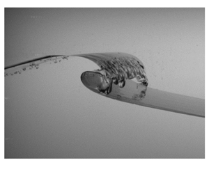
The value of  $\tau _b$ can be measured using either acoustical (Loewen & Melville Reference Loewen and Melville1991; Melville Reference Melville1994; Drazen et al. Reference Drazen, Melville and Lenain2008) or optical techniques (Tian et al. Reference Tian, Perlin and Choi2010, Reference Tian, Perlin and Choi2012). The former measures the acoustically active phase of wave breaking when bubbles are formed or fragmented in the turbulent two-phase flow (Deane & Stokes Reference Deane and Stokes2002). The optical technique relies on using visual features of breaking waves often derived from digital images. In this study, $\tau _b$ is measured using digital images of the breaking wave captured through the side glass panel of the wave flume. The value of $\tau _b$ is the time between incipient breaking identified as when the wave front becomes vertical and when the breaking front ceases to move forward in the direction of breaking. An example of the progression is shown in figure 10.
Frames of a breaking wave group of  $\gamma =2$ and $A(x_5)=96$ mm taken at different times during breaking. Incipient breaking and the end of breaking are indicated in the first and last images, the times of which are used to calculate the breaking duration.

Figures 11(a) and 11(b) show the variation of  $\tau _b$ and $\epsilon _b$ with $S_p$, respectively. For a given value of $S_p$, lower $\gamma$ wave groups break for longer than the higher $\gamma$ wave groups, indicating a bandwidth dependence. This result stems directly from the fact that breaking waves generated with the more broadband, lower $\gamma$, wave spectra break at a lower value of $S_p$. The net result is that the relationship between $\epsilon _b$ and $S_p$ shows a diminished bandwidth influence, stemming from a comparable bandwidth dependence in both $\tau _b$ and $\Delta E_{br}$. The same values of $\tau _b$ and $\epsilon _b/B$ are also plotted against $S_s$ in figures 11(c) and 11(d), in which the data of Tian et al. (Reference Tian, Perlin and Choi2010) (referred to as TPC10) are included for direct comparison. In contrast to figure 11(a), no clear bandwidth dependence between $\tau _b$ and $S_s$ is found. Coupled with the results in figure 9(e), $\epsilon _b/B$ shows little bandwidth dependence when plotted against $S_s$.
Plots of breaking duration,  $\tau _b$, against (a) $S_p(x_1)$ and (c) $S_s(x_1)$, and plots of breaking wave energy dissipation rate per unit flume width, $\epsilon _b/B$, against (b) $S_p(x_1)$ and (d) $S_s(x_1)$. In (c,d), experimental values from Tian et al. (Reference Tian, Perlin and Choi2010) are shown as TPC10. The dashed black lines in (b,d) represent the best-fit linear model given in (4.3) and (4.4), respectively.

The best-fit linear relationship of  $\epsilon _b/B$ with $S_p$ and $S_s$ shown in figures 11(b) and 11(d), respectively, are given as
 \begin{equation} \epsilon_b/B = (49.7\pm2.86)[S_p(x_1)-(0.23\pm0.02)], \end{equation}
and
 \begin{equation} \epsilon_b/B = (48.2\pm3.05)[S_s(x_1)-(0.27\pm0.02)], \end{equation}
with corresponding  $R^2$ values of 0.87 and 0.86. These two best fit lines have a similar slope, but different breaking onsets corresponding to $S_p \approx 0.23$ and $S_s \approx 0.27$ which are marginally lower than the value of $S_p$ at breaking onset estimated directly from the data (see table 2 and corresponding discussion). In figures 11(c) and 11(d), the range of the reported values of $\tau _b$ and $\epsilon _b/B$ are generally comparable to the results of TPC10, and any differences in values may be due to different underlying wave spectra employed across the two studies.
The coefficients in the power-law scaling of (4.7) for different  $\gamma$ using $S_p$ measured at $x_1$. Also included here are the 95 % confidence intervals of the fit coefficients with the corresponding $R^2$ values of the fitting curves; $S_p$ onset, $S_s$ onset and $S_n$ onset in the last three columns represent the estimated wave group steepness at breaking onset by taking the average steepness value of the largest non-breaking wave and incipient breaking wave at $x_1$.

4.5. Bandwidth effect on  $b$ and its parameterisation

For unidirectional breaking waves the breaking strength parameter,  $b$, is defined to be proportional to the energy dissipation rate per unit wave front length divided by the phase speed of the breaking wave ( $C$) raised to the fifth power. This is given by Duncan (Reference Duncan1981) as
 \begin{equation} b =\frac{\epsilon_b g}{\rho B C^5} , \end{equation}
where  $b$ can be determined in a relatively straightforward manner in laboratory studies for individual breaking waves. Following (4.2), if $b$ and $C$ are known the rate of energy dissipation can be calculated for individual breaking waves. Previous studies have used different definitions of $C$ to calculate $b$ and these can be broadly categorised into spectrally determined phase speeds and locally measured phase speeds, with each having multiple interpretations (Qiao & Duncan Reference Qiao and Duncan2001; Banner & Peirson Reference Banner and Peirson2007; Drazen et al. Reference Drazen, Melville and Lenain2008; Tian et al. Reference Tian, Perlin and Choi2010; Allis Reference Allis2013; Derakhti & Kirby Reference Derakhti and Kirby2016; Derakhti et al. Reference Derakhti, Banner and Kirby2018). Given the fundamental role of $C$ in (4.5), it is important to clearly state how it is determined here.
In this study we use  $C = 0.85 C_s$ where $C_s$ is calculated using the measurements at $x_1$ following Tian et al. (Reference Tian, Perlin and Choi2010):
 \begin{equation} C_s = \frac{2 {\rm \pi}f_s}{k_s}. \end{equation}
The coefficient 0.85 is used to approximate the initial incipient breaking wave phase speed following the experimental work of Allis (Reference Allis2013) and Tian et al. (Reference Tian, Perlin and Choi2010) and the numerical work of Derakhti & Kirby (Reference Derakhti and Kirby2016). Other studies that have employed a constant steepness spectrum have used the linearly predicted phase speed of the central frequency of the spectrum (Drazen et al. Reference Drazen, Melville and Lenain2008; Sinnis et al. Reference Sinnis, Grare, Lenain and Pizzo2021).
The calculated values of  $b$ are plotted against $S_p(x_1)$ in figure 12(a) and demonstrate a clear bandwidth influence. For a given value of $S_p$, $b$ is greater for breaking waves generated with broadband wave spectra for which breaking onset occurs at smaller values of $S_p$ as discussed in § 4.3. This same bandwidth dependence is not evident in figure 11(b), implying that the bandwidth dependence in $b(S_p)$ found here originates directly from the values of $C$ used in (4.5).
Plots of breaking strength parameter across all  $\gamma$ against different measures of wave group steepness. In (a), the dashed lines represent the polynomial best-fit lines to the data of each $\gamma$ following (4.7). In (b), values of $b$ are plotted against $S_s$ measured at $x_1$. The solid line and the dashed line depict equations (4.8) and (4.9), respectively. The breaking onset of $S_s=0.31$ given by Derakhti & Kirby (Reference Derakhti and Kirby2016) is denoted by the vertical grey line. Black squares and thick magenta circles are the experimental data from Tian et al. (Reference Tian, Perlin and Choi2010) (TPC10) and numerical data from Derakhti & Kirby (Reference Derakhti and Kirby2016) (DK16-a, computational reproduction of some of the wave conditions in Tian et al. Reference Tian, Perlin and Choi2010), respectively. In (c), values of $b$ are recalculated according to the energy dissipation approach of Drazen et al. (Reference Drazen, Melville and Lenain2008) except that the breaking phase speed, which was equal to the phase speed of the central frequency in Drazen et al. (Reference Drazen, Melville and Lenain2008), is reformulated in this dataset. Also shown here are data from Drazen et al. (Reference Drazen, Melville and Lenain2008) (D08, experimental), Melville (Reference Melville1994) (M94, experimental) and Derakhti & Kirby (Reference Derakhti and Kirby2016) (DK16-b, numerical reproduction of some breaking wave conditions of Rapp & Melville Reference Rapp and Melville1990; Drazen et al. Reference Drazen, Melville and Lenain2008). The use of target $S_n$ in (c) is for consistency with other studies. The grey solid line represents the empirical formulation of $b$ from Romero, Melville & Kleiss (Reference Romero, Melville and Kleiss2012).

Following the inertial scaling arguments in Drazen et al. (Reference Drazen, Melville and Lenain2008) and the subsequent development in Romero et al. (Reference Romero, Melville and Kleiss2012) the variation of  $b$ as a function of wave group steepness is suggested to follow the form
 \begin{equation} b=c_1(S-c_2)^{c_3}. \end{equation}
Based on the physical argument presented in Drazen et al. (Reference Drazen, Melville and Lenain2008),  ${c_3} = 2.5$ when using the target linear maximum wave group steepness $S_n$. This was further used in Romero et al. (Reference Romero, Melville and Kleiss2012) using a compilation of laboratory data, while other studies have chosen to keep ${c_3}$ as a free parameter (e.g. Derakhti & Kirby Reference Derakhti and Kirby2016) when fitting (4.7).
Equation (4.7) has been fitted in a least-mean squares sense to the four bandwidth datasets where we have chosen to keep  $c_3$ as a free parameter and have used $S = S_p$ measured at $x_1$. These fits are depicted in figure 12(a), and the resulting parameterisations are presented in table 2. The value of the fit coefficient $c_2$ can be interpreted as the value of $S_p$ at breaking onset and increases from 0.19 to 0.24 as $\gamma$ increases and bandwidth decreases. For comparison, table 2 also shows the best estimate of $S_p$ at breaking onset by taking the average value of $S_p$ for the largest non-breaking wave and smallest breaking wave as measured at $x_1$. As can be seen, these estimated values lie slightly above but within the 95 % confidence intervals of the $c_2$ coefficients, and follow the same trend with bandwidth. In addition, the exponent coefficient $c_3$ decreases as $\gamma$ increases and bandwidth decreases. While this trend is obvious and consistent, it should be noted that the associated 95 % confidence intervals are relatively large indicating that a larger dataset may be needed to constrain these values further. It is of interest to note that the value of $c_3$ is closest to the theoretical prediction of 2.5 from Drazen et al. (Reference Drazen, Melville and Lenain2008) for the $\gamma =1$ wave group examined here. For this dataset, the corresponding leading scaling coefficient, $c_1$, lies close to unity as suggested in the theoretical development in Drazen et al. (Reference Drazen, Melville and Lenain2008) (see their (2.9) and accompanying text).
As described in § 4.3 and shown in figures 9(b) and 9(e) the bandwidth-dependant scatter in our measured data reduces when using  $S_s$ compared with $S_p$. Following Tian et al. (Reference Tian, Perlin and Choi2010) and Derakhti & Kirby (Reference Derakhti and Kirby2016), we plot the breaking strength parameter as a function of $S_s$ in figure 12(b). Also shown are the experimental results of TPC10 and the numerical results of DK16-a for comparison. Good agreement is found across the compilation of datasets. However, most importantly, the bandwidth signature evident in figure 12(a) is now no longer present. This result is in qualitative agreement with Sinnis et al. (Reference Sinnis, Grare, Lenain and Pizzo2021) who achieved a better collapse of data when explicitly including a measure of bandwidth in their wave group steepness formulation (see their figure 8). However, as noted previously, we see different trends in terms of the bandwidth dependence on breaking onset as Sinnis et al. (Reference Sinnis, Grare, Lenain and Pizzo2021) with potential reasons explored in Appendix A.
Also shown in figure 12(b) are two fits of (4.7) to the data, where  $S = S_s$ and $c_3$ are set equal to 2.5 and 1, respectively. These fits are
 \begin{equation} b=(0.19\pm0.06)\left[S_s(x_1)-\left(0.11\pm0.04\right)\right]^{5/2} \end{equation}
and
 \begin{equation} b=(0.07\pm0.002)\left[S_s(x_1)-(0.27\pm0.004)\right], \end{equation}
with  $R^2$ values of 0.84 and 0.99, respectively. The linear model was chosen following the work of Tian et al. (Reference Tian, Perlin and Choi2010) and Derakhti & Kirby (Reference Derakhti and Kirby2016). The former study found $S_s$ to scale linearly with the locally measured steepness of incipient breaking waves. The latter numerically regenerated the experimental campaigns of Rapp & Melville (Reference Rapp and Melville1990), Drazen et al. (Reference Drazen, Melville and Lenain2008) and Tian et al. (Reference Tian, Perlin and Choi2012), which all employed dispersively focused breaking waves, and found the breaking strength parameter was best parameterised with a linear dependence on $S_s$.
Visually, both (4.8) and (4.9) follow the trend and magnitude of the bulk of the data very well despite the linear model having a higher correlation coefficient. However, the models give markedly different estimates for breaking onset of  $S_s = 0.11$ and $S_s = 0.27$, respectively. The latter value agrees well with both the numerical value of $S_s\approx 0.31$ from Derakhti & Kirby (Reference Derakhti and Kirby2016) and the experimentally derived value of $S_s = 0.28$ which is an average value from the four $\gamma$ values used in the present study. A small bandwidth-dependent trend in estimated value of $S_s$ at breaking onset is still observed, as presented in table 2, but is smaller to that found for $S_p$ and $S_n$ which are also listed in the same table. The overarching conclusion is that the breaking strength parameter scales linearly with $S_s$, which also helps to reduce, but not eliminate, any bandwidth-dependent sources of scatter.
As explained in § 3.2, the method to estimate energy dissipation used here is different to that outlined in the experimental study of Drazen et al. (Reference Drazen, Melville and Lenain2008). To provide a direct comparison between our results and those of Drazen et al. (Reference Drazen, Melville and Lenain2008), we recalculated the breaking wave energy dissipation and breaking strength parameter following the method outlined in Drazen et al. (Reference Drazen, Melville and Lenain2008), with the caveat that different breaking wave phase speeds are used because of the fundamental differences in the underlying spectra used. Figure 12(c) shows that the values of  $b$ as a function of target $S_n$ in the present study agree very well with those from Drazen et al. (Reference Drazen, Melville and Lenain2008), Melville (Reference Melville1994) and Derakhti & Kirby (Reference Derakhti and Kirby2016). These values of $b$ are up to a factor of between three and five greater than those presented in figures 12(a) and 12(b). Furthermore, our data follow well the trend and magnitude of the semi-empirical 2.5 power law given by Romero et al. (Reference Romero, Melville and Kleiss2012) for all wave group steepness except those close to breaking onset.
5. Concluding remarks
An experimental investigation of two-dimensional breaking waves with JONSWAP-type underlying wave spectra has been described. The present study has highlighted the role of bandwidth on the evolution of spectral energy distribution and characteristic wave group velocity in non-breaking and breaking wave groups, and additionally on energy dissipation, energy dissipation rate and the breaking strength parameter in breaking wave groups. These quantities have been examined in the context of three different measures of wave group steepness with each incorporating the bandwidth differently. The key results are summarised as follows.
(i) Definitions of wave steepness and their implications. The definition of wave group steepness adopted plays a critical role when evaluating potential bandwidth effects in wave breaking. Three definitions of wave group steepness were adopted in this study:
$S_n$, $S_s$ and $S_p$. Of these, only $S_p$ remained constant for a given value of linear amplitude sum ($A$) when changes to bandwidth were made. We have used $S_p$ to identify the role of bandwidth in the breaking waves studied here. Furthermore, $S_p$ does not show consistent variation with proximity to the breaking location at the positions measured here. In contrast, $S_n$ is more sensitive to both bandwidth and measurement location because increases in the amplitudes of high-frequency components with increasing proximity to the breaking location is more readily captured by $S_n$. While $S_s$ is also dependent on bandwidth, its value also remains largely constant along the wave flume due to very little spectral energy present at high frequencies for JONSWAP-type spectra.(ii) Spectral energy distribution. Two regimes of spectral energy evolution in breaking wave groups are found which are partitioned at a threshold frequency which is roughly equal to
$0.95f_p$. At frequencies $f \ge 0.95f_p$ wave breaking results in an energy loss which is concentrated over an increasingly narrow range of frequencies as $\gamma$ increases from $\gamma = 1$ to $\gamma = 4$. The peak energy loss clearly lies close to $f_p$ for the $\gamma = 2, 3$ and $4$ wave groups, but occurs at a frequency higher than $f_p$ for the wave groups of $\gamma = 1$. We speculate that this notable result for $\gamma = 1$ is attributed to the markedly different corresponding wave steepness spectrum. Below $0.95f_p$ there is a consistent bandwidth-dependent increase of spectral energy in the breaking wave groups as the wave groups become steeper. However, this is not clearly observed in the non-breaking wave groups. This result implies that an additional mechanism of nonlinear transfer of energy to lower frequencies ($f \le 0.95f_p$) occurs in breaking wave groups that is not present in steep but non-breaking wave groups. The net result causes a downshift of the peak frequency to lower values in the breaking wave groups.(iii) Characteristic group velocity evolution. Measurements of
$C_{gs}$ at different locations show an increase in $C_{gs}$ for both non-breaking and breaking wave groups as the groups propagate along the wave flume. Upstream of the breaking location, the value of $C_{gs}$ increases consistently for all breaking and non-breaking wave groups. However, at the upstream wave gauge closest to the breaking location and the wave gauges downstream of the breaking location, there is a noticeable increase in $C_{gs}$ for the breaking wave groups only. The net increase in $C_{gs}$ across the control volume for breaking waves is proportional to wave group steepness with the greatest increase found in the lowest $\gamma$ value, or most broadband, breaking wave groups. This is because these breaking wave groups dissipate more fractional energy over a broader frequency range compared with wave groups of higher $\gamma$. The overall maximum increase in $C_{gs}$ is between 5 % and 7 % which is comparable to values of 5 % and 10 % reported in previous studies.(iv) Breaking wave onset, energy dissipation and its rate. Breaking wave onset, fractional energy loss and absolute energy loss are bandwidth dependent. This dependence is more easily seen when using
$S_p$, in contrast to both $S_s$ and $S_n$. Breaking onset was characterised using the wave group steepness measured at the start of the control volume and occurs between $S_p \approx 0.22$ rand $S_p \approx 0.29$ for the $\gamma = 1$ and $\gamma = 4$ wave groups, respectively. Further studies that examine any bandwidth dependence in local wave steepness at breaking are needed.We find that breaking wave groups of broadband spectra dissipate more fractional energy than those generated from narrowband spectra at a given value of
$S_p$, primarily due to the earlier breaking onset. In terms of absolute energy loss, while a bandwidth dependence with $S_p$ can still be observed, it is reduced compared with the trends observed in the fractional energy loss. These bandwidth-dependent trends in fractional energy loss are comparatively reduced when considering $S_s$ or $S_n$ in place of $S_p$, but not absent. In contrast to the fractional energy loss results, the rate of energy dissipation, which depends on both the absolute energy loss and a characteristic timescale of breaking ($\tau _b$), is not found to exhibit any clear bandwidth dependence with $S_p$. This is because at a given value of $S_p$ both absolute energy loss and $\tau _b$ are higher for lower $\gamma$ wave groups thereby effectively removing a clear bandwidth dependence in their ratio. An important conclusion is that the average rate of energy dissipation of breaking waves is linearly related to both $S_p$ and $S_s$, and does not exhibit any appreciable bandwidth dependence for the wave groups considered here, over and above the bandwidth-dependent breaking onset mentioned previously.(v) Breaking strength parameter and its parameterisation. The laboratory data show a strong dependence between bandwidth and the breaking strength parameter,
$b$, which emerges because the breaking speed $C_s$ decreases with increasing bandwidth. The relationship between $b$ and $S_p$ becomes increasingly nonlinear as bandwidth increases. When parameterised in terms of $S_s$, bandwidth-dependent scatter in values of $b$ is markedly reduced. A linear relationship between $b$ and $S_s$ is found which corroborates the numerical result of Derakhti & Kirby (Reference Derakhti and Kirby2016) and indirectly agrees with data from Tian et al. (Reference Tian, Perlin and Choi2010). Furthermore, when following the approach of Drazen et al. (Reference Drazen, Melville and Lenain2008) of using target $S_n$ to characterise variation in $b$, our data lie within the scatter of previous datasets and agree well the semi-empirical power-law scaling of 2.5 proposed in Romero et al. (Reference Romero, Melville and Kleiss2012).


Finally, the present study used a single value of  $k_p$, and future work should include a larger range of $k_p$ to further evaluate bandwidth dependencies. Furthermore, as suggested by one of the reviewers, additional work where target $S_n$ is kept constant and bandwidth varied would provide additional information on the interdependence of these two parameters and further insight into the role of bandwidth changes on energy dissipation in breaking waves.
Acknowledgements
The authors thank the three reviewers for their suggestions, corrections and useful comments which improved the manuscript. A.H.C. would like to thank Professor C. Swan for hosting him at Imperial College London as a visiting scientist in 2015 when the experiments were carried out.
Funding
The experiments reported here were funded by the National Science Foundation (grant number OCE-1434866) while A.H.C. was a visiting researcher in the Department of Civil and Environmental Engineering at Imperial College London from 2015 to 2016. A.H.C. received further funding from a Royal Society Shooter International Fellowship and a NERC Standard Grant (grant number NE/T000309/1). While E.M.P. was at Imperial College London, he was supported by NERC (grant number NE/T000309/1). R.C. was supported with a Skempton PhD fellowship from the Department of Civil and Environmental Engineering, Imperial College London.
Declaration of interests
The authors report no conflict of interest.
Author contributions
RC: Conceptualisation, Methodology, Data analysis, Writing — Original Draft, Writing — Review & Editing; EMP: Methodology, Writing — Review & Editing; AHC: Conceptualisation, Data Collection, Methodology, Data analysis, Writing — Review & Editing, Supervision, Funding acquisition.
Appendix A. Different bandwidth definitions and their implications
As mentioned in § 1, while the peak enhancement factor,  $\gamma$, is not a direct measure of bandwidth, different values of $\gamma$ do change the bandwidth of a wave spectrum leading to changes to the corresponding steepness spectrum. In what follows, we describe various definitions of bandwidth used in the literature and examine how their values change with $S_p, S_n, S_s$ and $\gamma$.
Following usage in the literature (e.g. Wu & Yao Reference Wu and Yao2004), we classify the bandwidth as either spectral bandwidth or frequency bandwidth. The former is calculated using various moments of the wave spectrum and so explicitly incorporates a measure of the energy of the wave spectrum. In the case of frequency bandwidth, it has been defined both with a measure of the spectral energy and without as described in the following.
Two common spectral bandwidth definitions, as outlined in Saulnier et al. (Reference Saulnier, Clément, Falcão, Pontes, Prevosto and Ricci2011), are
 \begin{equation} \varepsilon_{1}=\sqrt{\frac{m_{1} m_{-1}}{m_{0}^{2}}-1}, \end{equation}
proposed by Smith, Venugopal & Wolfram (Reference Smith, Venugopal and Wolfram2006), and
 \begin{equation} \nu=\sqrt{\frac{m_{0} m_{2}}{m_{1}^{2}}-1}, \end{equation}
initially used in Longuet-Higgins (Reference Longuet-Higgins1957). In these two definitions, we use  $m_n = \int _{f_p/2}^{3f_p} f^n S_{\eta \eta }(\,f) \, {\rm d}f$ to represent the $n$th spectral moment. Equation (A1) is more sensitive to the lower-frequency components, whereas (A2) is more influenced by the higher-frequency components due to the presence of $m_{2}$. As seen in figures 13(a)–13(f) both $\varepsilon _{1}$ and $\nu$ are dependent on wave group steepness and, strikingly, inversely proportional to $\gamma$ value. Moreover, there is no unique relationship between these measures of bandwidth and $\gamma$ value.
Plots of  $\varepsilon _{1}$, $\nu$, $1/Q_p$, $\Delta f / f_{s}, \Delta f/f_p$ and $(\,f_N - f_1)/ f_{s}$ against different measures of wave group steepness. These quantities are all calculated based on the measurements taken at $x_1$. Datapoints with black lines specifically indicate breaking wave groups.

Rao (Reference Rao1988) used the inverse of the so-called peakedness parameter ( $Q_p$) proposed by Goda (Reference Goda1970) as a measure of spectral bandwidth,
 \begin{equation} Q_p=\frac{2}{m_{0}^2} \int^{f_N}_{f_1} f \left[S_{\eta\eta}(\,f)\right]^2 {\rm d}f, \end{equation}
where  $f_1$ and $f_N$ are the lowest and highest spectral frequencies of the wave spectrum. Therefore, a higher value of $Q_p$ represents a smaller spectral bandwidth. As seen in figures 13(g)–13(i) a similar dependence of $1/Q_p$ (and hence spectral bandwidth) with both wave group steepness and $\gamma$ value as $\varepsilon _{1}$ and $\nu$ is found, albeit with only a weak variation as a function of wave group steepness. Unlike $\varepsilon _{1}$ and $\nu$, however, any particular value of $1/Q_p$ is not associated with multiple $\gamma$ values and is just inversely proportional to $\gamma$.
On the other hand, the general form of frequency bandwidth is  $\Delta f / f_{x}$, where $\Delta f$ is typically the difference between two specific frequencies and $f_{x}$ is a characteristic frequency. As stated previously, frequency bandwidth may or may not incorporate the spectral energy distribution in its definition. In the former case, $\Delta f$ can be calculated as the bandwidth between two frequency components were the spectral energy level is one-half the peak value (e.g. Tian et al. Reference Tian, Perlin and Choi2010). In this regard, the one-half maximum frequency bandwidth explicitly relies on a measure of spectral energy distribution. Figures 13(j)–13(l) show the variation this bandwidth definition with wave group steepness and $\gamma$ value with $f_{x} = f_{s}$, where $f_{s}$ is defined in (3.3). While there is a small variation in $f_{s}$ as a function of wave group steepness, it is not discernible so $\Delta f / f_{s}$ may be considered independent of wave group steepness. Similarly, $\Delta f / f_{p}$ is also independent of wave group steepness as seen in figures 13(m)–13(o). Unlike the previous spectral bandwidth definitions, both $\Delta f/f_s$ and $\Delta f/f_p$ are exclusively inversely related to $\gamma$. In other words, for the spectra examined here, they play a similar role as $\gamma$ so either can be regarded as an equivalent measure of $\gamma$ which can be used to determine the bandwidth of JONSWAP-type spectra.
The final definition of frequency bandwidth has been almost exclusively used for constant steepness and/or constant amplitude spectra. It defines  $\Delta f = f_N - f_1$ and is routinely normalised by the central frequency, $f_c$ of the wave spectrum. This definition has been used widely in many studies such as Wu & Yao (Reference Wu and Yao2004), Drazen et al. (Reference Drazen, Melville and Lenain2008), Liang et al. (Reference Liang, Zhang, Sun and Chang2017), Sinnis et al. (Reference Sinnis, Grare, Lenain and Pizzo2021) and Pizzo et al. (Reference Pizzo, Murray, Smith and Lenain2021). It it important to note that this definition does not incorporate the energy of, nor its distribution within, the underlying wave spectrum. In other words, $(\,f_N - f_1)/f_c$ may be fixed even though the underlying steepness spectrum changes which can be achieved by modifying the $\gamma$ value in JONSWAP-type spectra (see figure 1b), or by changing the slope of the steepness spectrum (Wu & Yao Reference Wu and Yao2004). Consequently, it is suggested that it is important to incorporate the spectral energy distribution in the bandwidth definition when examining the bandwidth effect on a variety of wave spectra. Given that the concept of a central frequency does not apply for the JONSWAP-type spectra used in this study, $f_{x} = f_{s}$ is used. Figures 13(p)–13(r) show that there are striking differences in the relationship between $(\,f_N - f_1) / f_s$ and all other measures of bandwidth that do incorporate a measure of spectral energy. First, $(\,f_N - f_1) / f_s$ is directly proportional to $\gamma$ indicating that its value is larger for more narrowband wave spectra, in contrast to all other measures of bandwidth. Second, there is a general decrease in its value with increasing wave slope for all breaking waves, although this dependence is secondary and weak.
Appendix B. The relationship between $S_p$, $S_s$ and $S_n$


The relationship between all three measures of wave group steepness measured at gauge 1 are shown in figure 14. The relationships are quantified in table 3.
Plots of the relationships between different measures of wave group steepness at  $x_1$.

The least-mean-squares relationships between all three measures of wave group steepness measured at  $x_1$. Values in parentheses represent 95 % confidence intervals on fit coefficients.


 Open access

