





1. Introduction, main results, and discussion
Let $\{Y_n\}$
be a branching process with the offspring distribution
$\{Y_n\}$
be a branching process with the offspring distribution $\{p_k\}$
and with immigration governed by the distribution
$\{p_k\}$
and with immigration governed by the distribution $\{q_k\}$
. A mathematically rigorous description can be as follows. Let
$\{q_k\}$
. A mathematically rigorous description can be as follows. Let $\{\xi_{n,j}\}$
be independent random variables with distribution
$\{\xi_{n,j}\}$
be independent random variables with distribution $\{p_k\}$
and let
$\{p_k\}$
and let $\{\eta_n\}$
be independent random variables with distribution
$\{\eta_n\}$
be independent random variables with distribution $\{q_k\}$
. We assume also that the sequences
$\{q_k\}$
. We assume also that the sequences $\{\xi_{n,j}\}$
and
$\{\xi_{n,j}\}$
and $\{\eta_n\}$
are independent from each other. Then the process
$\{\eta_n\}$
are independent from each other. Then the process $\{Y_n\}$
can be defined by the following recursive equation:
$\{Y_n\}$
can be defined by the following recursive equation:
 \begin{equation}Y_{n+1}=\sum_{j=1}^{Y_n}\xi_{n+1,j}+\eta_{n+1},\quad n\geq 0.\end{equation}
The starting point $Y_{0}$
can be deterministic or random; one only assumes that
$Y_{0}$
can be deterministic or random; one only assumes that $Y_{0}$
is independent of the sequences
$Y_{0}$
is independent of the sequences $\{\xi_{n,j}\}$
and
$\{\xi_{n,j}\}$
and $\{\eta_n\}$
.
$\{\eta_n\}$
.
In this paper we shall consider only critical processes, that is,
 \begin{equation}\sum_{k=1}^{\infty} kp_{k}=1.\end{equation}
Furthermore, we shall always assume that
 \begin{equation}B\,:\!=\, \sum_{k=1}^\infty k(k-1)p_{k}\in(0,\infty)\quad\text{and}\quad\lambda\,:\!=\, \sum_{k=1}^{\infty} kq_{k}\in(0,\infty).\end{equation}
It is worth mentioning that the strict positivity of $\sum_{k=1}^{\infty} kq_{k}$
means that the random variables
$\sum_{k=1}^{\infty} kq_{k}$
means that the random variables $\{\eta_n\}$
are non-degenerate and, consequently, standard Galton–Watson processes are excluded.
$\{\eta_n\}$
are non-degenerate and, consequently, standard Galton–Watson processes are excluded.
Seneta [Reference Seneta8] has shown that if (2) and (3) are valid then ${{2Y_{n}}/{(Bn)}}$
converges weakly towards a gamma distribution. More precisely, for every
${{2Y_{n}}/{(Bn)}}$
converges weakly towards a gamma distribution. More precisely, for every $x\gt 0$
we have
$x\gt 0$
we have
 \begin{equation}\lim_{n\to\infty}\mathbb P\biggl(\dfrac{2Y_{n}}{Bn}\leq x\biggr)=\dfrac{1}{\Gamma(\gamma)}\int_0^x u^{\gamma-1}{\mathrm{e}}^{-u}\,{\mathrm{d}} u,\end{equation}
where
 \begin{align*}\gamma\,:\!=\, \dfrac{2\lambda}{B}.\end{align*}
Seneta considers the case $Y_0=1$
only, but it is very easy to check that his arguments work for all starting distributions.
$Y_0=1$
only, but it is very easy to check that his arguments work for all starting distributions.
Mellein [Reference Mellein5] has proved the corresponding local limit theorem. Assuming that
 \begin{equation}\sum_{k=1}^\infty (k^2\log k) p_{k}\lt\infty\quad\text{and}\quad\sum_{k=1}^\infty (k\log k) q_{k}\lt\infty,\end{equation}
he has shown that, for every fixed i,
 \begin{equation}\mathbb P(Y_{n}=k\mid Y_{0}=i) \sim\dfrac{1}{\Gamma(\gamma)}\biggl(\dfrac{2}{B}\biggr)^{\gamma}\dfrac{k^{\gamma-1}}{n^\gamma}{\mathrm{e}}^{-2k/(Bn)}\end{equation}
as $n,k\to\infty$
and
$n,k\to\infty$
and $k/n$
remains bounded.
$k/n$
remains bounded.
Since the moments in (5) do not show up in the asymptotics (6), it is natural to ask whether these conditions are needed for the local limit theorem. This question is our main motivation to consider lower deviation probabilities for $Y_{n}$
. More precisely, we are going to determine the asymptotic behaviour of the probabilities
$Y_{n}$
. More precisely, we are going to determine the asymptotic behaviour of the probabilities $\mathbb P(Y_{n}\leq k)$
and
$\mathbb P(Y_{n}\leq k)$
and $\mathbb P(Y_{n}=k)$
in the case when
$\mathbb P(Y_{n}=k)$
in the case when $k\to\infty$
but
$k\to\infty$
but $k={\mathrm{o}} (n)$
for processes satisfying (2) and (3) only. Comparing asymptotics for local probabilities with the corresponding values of the limiting density, we can then conclude whether the extra condition (5) is really needed for the validity of (6).
$k={\mathrm{o}} (n)$
for processes satisfying (2) and (3) only. Comparing asymptotics for local probabilities with the corresponding values of the limiting density, we can then conclude whether the extra condition (5) is really needed for the validity of (6).
Theorem 1. Assume that (2) and (3) hold. Then there exists a slowly varying function $L(x)$
such that, for every fixed
$L(x)$
such that, for every fixed $i\ge0$
,
$i\ge0$
,
 \begin{equation}\mathbb P(Y_{n}\leq k\mid Y_0=i)\sim\dfrac{1}{\Gamma(\gamma+1)}\biggl(\dfrac{2}{B}\biggr)^{\gamma}\dfrac{k^\gamma L(k)}{n^\gamma L(n)}\end{equation}
for $k\to\infty$
and
$k\to\infty$
and $k={\mathrm{o}} (n)$
. If, additionally,
$k={\mathrm{o}} (n)$
. If, additionally, $\{p_{k}\}$
and
$\{p_{k}\}$
and $\{q_{k}\}$
are aperiodic, then, for every fixed
$\{q_{k}\}$
are aperiodic, then, for every fixed $i\ge0$
,
$i\ge0$
,
 \begin{equation}\mathbb P(Y_{n}=k\mid Y_0=i)\sim\dfrac{1}{\Gamma(\gamma)}\biggl(\dfrac{2}{B}\biggr)^{\gamma}\dfrac{k^{\gamma-1} L(k)}{n^{\gamma} L(n)}\end{equation}
for $k\to\infty$
such that
$k\to\infty$
such that $k={\mathrm{o}} (n)$
. Finally, for every fixed
$k={\mathrm{o}} (n)$
. Finally, for every fixed $k\ge 1$
there exists
$k\ge 1$
there exists $\mu_{k}\in[0,\infty)$
such that, as
$\mu_{k}\in[0,\infty)$
such that, as $n\to\infty$
,
$n\to\infty$
,
 \begin{equation}n^{\gamma} L(n)\,\mathbb P (Y_{n}=k\mid Y_0=i )\to\mu_{k}.\end{equation}
The function $L(x)$
converges to a positive constant provided that (5) holds. If
$L(x)$
converges to a positive constant provided that (5) holds. If
 \begin{align*}\sum_{k=1}^\infty (k^{2}\log k ) p_{k}\lt\infty\quad{and}\quad\sum_{k=1}^\infty (k\log k ) q_{k}=\infty,\end{align*}
then $L(n)$
tends to zero. Furthermore, if
$L(n)$
tends to zero. Furthermore, if
 \begin{align*}\sum_{k=1}^\infty (k^{2}\log k ) p_{k}=\infty\quad{and}\quad\sum_{k=1}^\infty (k\log k ) q_{k}\lt\infty,\end{align*}
then $L(n)$
tends to infinity.
$L(n)$
tends to infinity.
This result shows that (6) can fail if the moment conditions in (5) are not valid. This is quite different from the case of critical Galton–Watson processes. Nagaev and Wachtel [Reference Nagaev and Vakhtel6] have shown that the existence of the second moment is sufficient for the local limit theorem.
We conjecture that the domain of lower deviations is the only zone where one needs (5) for the local asymptotics (6). In other words, we believe that the following statement holds: if (2) and (3) are valid, then for every fixed $\varepsilon\gt 0$
we have
$\varepsilon\gt 0$
we have
 \begin{equation}\sup_{k\geq\varepsilon n}\biggl|n\mathbb P (Y_{n}=k )-\dfrac{1}{\Gamma(\gamma)}\biggl(\dfrac{2k}{Bn}\biggr)^{\gamma-1}{\mathrm{e}}^{-2k/(Bn)}\biggr|\to 0\quad \text{as $n\to\infty$.}\end{equation}
Noting that $u^{\gamma-1}{\mathrm{e}}^{-u}\to 0$
as
$u^{\gamma-1}{\mathrm{e}}^{-u}\to 0$
as $u\to 0$
for
$u\to 0$
for $\gamma\gt 1$
and combining (10) with the fact that
$\gamma\gt 1$
and combining (10) with the fact that $\mathbb{P}(Y_n=k)={\mathrm{o}} (n^{-1})$
for
$\mathbb{P}(Y_n=k)={\mathrm{o}} (n^{-1})$
for $k={\mathrm{o}} (n)$
(see Remark 1 at the end of the paper for the corresponding uniform bound), we get for
$k={\mathrm{o}} (n)$
(see Remark 1 at the end of the paper for the corresponding uniform bound), we get for $\gamma\gt 1$
the most standard version of the local limit theorem:
$\gamma\gt 1$
the most standard version of the local limit theorem:
 \begin{equation}\sup_{k\ge0}\biggl|n\mathbb P (Y_{n}=k )-\dfrac{1}{\Gamma(\gamma)}\biggl(\dfrac{2k}{Bn}\biggr)^{\gamma-1}{\mathrm{e}}^{-2k/(Bn)}\biggr|\to 0\quad \text{as $n\to\infty$.}\end{equation}
(Note that this relation is not stronger than (6), because for $k={\mathrm{o}} (n)$
we get only
$k={\mathrm{o}} (n)$
we get only $\mathbb P (Y_{n}=k )={\mathrm{o}} (n^{-1} )$
.)
$\mathbb P (Y_{n}=k )={\mathrm{o}} (n^{-1} )$
.)
Pakes [Reference Pakes7] has shown (9) under the condition (5). Therefore Theorem 1 generalizes the results of Mellein [Reference Mellein5] and Pakes [Reference Pakes7] to the whole class of processes satisfying (3).
Our Theorem 1 can be used to derive asymptotics for the so-called harmonic moments $\mathbb E[Y_n^{-r};\,Y_n\gt 0]$
in a rather simple way. This has been done by other means in Li and Zhang [Reference Li and Zhang4].
$\mathbb E[Y_n^{-r};\,Y_n\gt 0]$
in a rather simple way. This has been done by other means in Li and Zhang [Reference Li and Zhang4].
Our approach to lower deviation probabilities differs from that in the above-mentioned papers by Mellein and by Pakes. We first determine an optimal strategy which leads to atypically small values of $Y_{n}$
. This allows us to reduce our problem on small deviations to a problem on normal deviations, where one can use results known in the literature. To describe this optimal strategy, we introduce some additional notation. Let
$Y_{n}$
. This allows us to reduce our problem on small deviations to a problem on normal deviations, where one can use results known in the literature. To describe this optimal strategy, we introduce some additional notation. Let $\{Z_{n}^{(i)}\}$
,
$\{Z_{n}^{(i)}\}$
, $i\ge1$
be a sequence of independent Galton–Watson processes with offspring distribution
$i\ge1$
be a sequence of independent Galton–Watson processes with offspring distribution $\{p_{k}\}$
and with
$\{p_{k}\}$
and with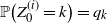 $\mathbb P \bigl(Z_{0}^{ (i )}=k \bigr)=q_{k}$
,
$\mathbb P \bigl(Z_{0}^{ (i )}=k \bigr)=q_{k}$
, $k\ge 0$
. It is immediate from (1) that if
$k\ge 0$
. It is immediate from (1) that if $Y_{0}=0$
then one can define
$Y_{0}=0$
then one can define $Y_n$
and
$Y_n$
and $\{Z_n^{(i)}\}$
on the same probability space so that
$\{Z_n^{(i)}\}$
on the same probability space so that
 \begin{equation}Y_{n}=\sum_{i=1}^{n} Z^{ (i )}_{n-i}\quad\text{almost surely}.\end{equation}
Now define
 \begin{equation}\theta_{n}\,:\!=\, \inf\bigl\{i\leq n\,\colon Z^{ (i )}_{n-i}\gt 0\bigr\}.\end{equation}
In words, $\theta_{n}$
is the first generation where immigrants have descendants at time n. We know from (4) that
$\theta_{n}$
is the first generation where immigrants have descendants at time n. We know from (4) that $Y_{n}$
is typically of size n and that a Galton–Watson process
$Y_{n}$
is typically of size n and that a Galton–Watson process $Z_{n}$
conditioned on non-extinction is also of order n. Thus it is quite plausible to assume that if we want to have only k particles in the nth generation, then
$Z_{n}$
conditioned on non-extinction is also of order n. Thus it is quite plausible to assume that if we want to have only k particles in the nth generation, then $\theta_{n}$
should be such that
$\theta_{n}$
should be such that $n-\theta_{n}$
is of order k. In the course of the proof of Theorem 1, we show that this strategy is indeed optimal.
$n-\theta_{n}$
is of order k. In the course of the proof of Theorem 1, we show that this strategy is indeed optimal.
A strategy that keeps the size of the process as small as possible, up to an appropriate time moment, is quite standard for branching processes. This type of behaviour is also optimal for lower deviations of supercritical Galton–Watson processes; see e.g. [Reference Fleischmann and Wachtel2].
Our paper is organized as follows. In Section 2 we provide some results about upper bounds for lower deviation probabilities. Section 3 contains estimates for the concentration function, and Section 4 gathers the proof of the main theorem.
In what follows, we shall use the symbols $c,c_k$
and
$c,c_k$
and $C,C_k$
to denote numbers which may depend on distributions
$C,C_k$
to denote numbers which may depend on distributions $\{p_k\}$
and
$\{p_k\}$
and $\{q_k\}$
only and may change their values from place to place.
$\{q_k\}$
only and may change their values from place to place.
2. Analysis of generating functions and some preliminary probabilistic estimates
Define $f (s )\,:\!=\, \sum_{k=0}^\infty p_{k}s^{k}$
and
$f (s )\,:\!=\, \sum_{k=0}^\infty p_{k}s^{k}$
and $h (s )\,:\!=\, \sum_{k=0}^\infty q_ks^k$
; here and in what follows,
$h (s )\,:\!=\, \sum_{k=0}^\infty q_ks^k$
; here and in what follows, $s\in\mathbb{C}$
. In other words, f(s) is the offspring generating function of the processes
$s\in\mathbb{C}$
. In other words, f(s) is the offspring generating function of the processes $\{Y_{n}\}$
and
$\{Y_{n}\}$
and $\{Z_{n}^{ (i )}\}$
, and h(s) is the generating function of the number of immigrants in
$\{Z_{n}^{ (i )}\}$
, and h(s) is the generating function of the number of immigrants in $\{Y_{n}\}$
and of
$\{Y_{n}\}$
and of $Z_{0}^{ (i )}$
. Let
$Z_{0}^{ (i )}$
. Let $f_{n} (s )$
denote the nth iteration of f.
$f_{n} (s )$
denote the nth iteration of f.
In this section we shall always assume that $Y_0=0$
.
$Y_0=0$
.
It is immediate from (12) that
 \begin{align*}H_n(s)\,:\!=\, \mathbb E \big[s^{Y_n} \big]=\prod_{k=0}^{n-1}h(f_k(s)),\quad n\ge1.\end{align*}
For the random variable $\theta_{n}$
defined in (13), we then have, for every
$\theta_{n}$
defined in (13), we then have, for every $l\leq n$
,
$l\leq n$
,
 \begin{equation*} \mathbb P (\theta_{n}\gt l )=\prod_{i=1}^l\mathbb P\bigl(Z_{n-i}^{(i)}=0\bigr) =\prod_{i=1}^{l} h (f_{n-i}(0) ) =\prod_{k=n-l}^{n-1}h (f_{k}(0) ) \end{equation*}
and
 \begin{align} \mathbb P (\theta_n=l ) &=\mathbb P (\theta_n\gt l-1 )-\mathbb P (\theta_n\gt l ) = (1-h (f_{n-l}(0) ) )\prod_{k=n-l+1}^{n-1}h (f_{k}(0) ). \end{align}
Define
 \begin{align*} F(0)\,:\!=\, 1\quad\text{and}\quad F(n)\,:\!=\, \prod_{k=0}^{n-1}h(f_k(0)),\quad n\geq 1. \end{align*}
Then
 \begin{equation*} \mathbb P(\theta_n\gt l)=\dfrac{F(n)}{F (n-l )}, \quad l\in\{0,1,\ldots, n\} \end{equation*}
and
 \begin{equation*} \mathbb P (\theta_n=l )= (1-h (f_{n-l}(0) ) )\dfrac{F(n)}{F(n-l+1)}, \quad l\in\{1,2,\ldots, n\}. \end{equation*}
The first purpose of this section is to determine the asymptotic behaviour of F(n). We show that this function is regularly varying at infinity and derive some properties of the corresponding slowly varying function.
We begin with a simple lemma, which is an easy consequence of the Taylor formula.
Lemma 1. For $ |s |\le 1$
, it holds that
$ |s |\le 1$
, it holds that
 \begin{equation} \log h (s )=-h'(1) (1-s )+{\mathrm{o}} (s-1 ), \quad s\to 1,\end{equation}
where $\log$
denotes the principal value of the logarithm.
$\log$
denotes the principal value of the logarithm.
Proof. We start by noting that for $|s|\lt1$
,
$|s|\lt1$
,
 \begin{align*} \dfrac{h(1)-h(s)}{1-s} =\sum_{k=1}^\infty q_k\dfrac{1-s^k}{1-s} =\sum_{k=1}^\infty q_k\sum_{j=0}^{k-1}s^j. \end{align*}
By the triangle inequality,
 \begin{align*} \biggl|\dfrac{h(1)-h(s)}{1-s}-h'(1)\biggr| \le\sum_{k=1}^\infty q_k\Biggl|\sum_{j=0}^{k-1}s^j-k\Biggr|. \end{align*}
For every fixed k, we have
 \begin{align*}\Biggl|\sum_{j=0}^{k-1}s^j-k\Biggr|\to0\quad\text{as $s\to1$.}\end{align*}
Furthermore, for every k we have the bound
 \begin{align*}\Biggl|\sum_{j=0}^{k-1}s^j-k\Biggr|\le 2k,\quad |s|\le1.\end{align*}
The assumption $\sum_{k=1}^\infty kq_k\lt\infty$
allows us to apply the dominated convergence theorem, which gives
$\sum_{k=1}^\infty kq_k\lt\infty$
allows us to apply the dominated convergence theorem, which gives
 \begin{align*}\Biggl|\dfrac{h(1)-h(s)}{1-s}-h'(1)\Biggr|\to0\quad\text{as $s\to1$.}\end{align*}
In other words,
 \begin{align*}h(s)=h(1)-h'(1)(1-s)+{\mathrm{o}} ((1-s)).\end{align*}
Taking the logarithm, we get the desired representation.
The following lemma describes the asymptotic behaviour of F(n).
Lemma 2. There exists a slowly varying function $L(x)$
such that
$L(x)$
such that
 \begin{align*}\dfrac{1}{n^\gamma F(n)}\sim L(n)\quad{as}\ n\to\infty.\end{align*}
Proof. According to the representation theorem for slowly varying functions, it suffices to show that ${{1}/{(n^\gamma F(n))}}$
is asymptotically equivalent to a function L(n) of the following form:
${{1}/{(n^\gamma F(n))}}$
is asymptotically equivalent to a function L(n) of the following form:
 \begin{equation} L(n)=c\exp\biggl\{\int_{1}^{n}\dfrac{\tau (y )}{y}\,{\mathrm{d}} y \biggr\},\end{equation}
where $\tau$
is a bounded function such that
$\tau$
is a bounded function such that $\tau (y ) \to 0$
as
$\tau (y ) \to 0$
as $y \to \infty$
, and
$y \to \infty$
, and $c\gt 0$
.
$c\gt 0$
.
We infer from (15) that
 \begin{equation} \log h (s )=-h'(1) (1-s )+ (s-1 )\alpha (s ),\quad |s|\le 1,\end{equation}
where $\alpha (s )\to 0$
as
$\alpha (s )\to 0$
as $s \to 1$
and
$s \to 1$
and $|s|\le 1$
.
$|s|\le 1$
.
Due to the condition $B\lt\infty$
,
$B\lt\infty$
,
 \begin{equation}1-f_{j}(0)=\dfrac{2}{Bj}+\dfrac{\epsilon_{j}}{j},\end{equation}
where $\epsilon_{j} \to 0$
as
$\epsilon_{j} \to 0$
as $j \to \infty$
. Combining this with (17), we have, as
$j \to \infty$
. Combining this with (17), we have, as $n\to\infty$
,
$n\to\infty$
,
 \begin{align*}\begin{aligned}n^{\gamma} F(n) & = n^{\gamma}\exp\Biggl\{\sum_{j=0}^{n-1}\log h (f_{j}(0) ) \Biggr\}\\& = n^{\gamma}\exp\Biggl\{-h'(1)\sum_{j=0}^{n-1} (1-f_{j}(0) )-\sum_{j=1}^{n} (1-f_{j}(0) )\alpha (f_{j}(0) ) \Biggr\} \\& = n^{\gamma}\exp\Biggl\{-\dfrac{2h'(1)}{B}\sum_{j=1}^{n}\dfrac{1}{j} \Biggr\} \exp\Biggl\{\sum_{j=1}^{n}\biggl(\dfrac{-h'(1)\epsilon_{j}}{j}-\dfrac{({{2}/{B}}+\epsilon_{j})\alpha(f_{j}(0))}{j}\biggr) \Biggr\}\\& \sim n^{\gamma}C\exp \{-\gamma \log n \} \exp\Biggl\{-\sum_{j=1}^{n}\dfrac{ (h'(1)\epsilon_{j}+({{2}/{B}}+\epsilon_{j})\alpha (f_{j}(0) ) )}{j} \Biggr\} \\& = C\exp\Biggl\{-\sum_{j=1}^{n}\dfrac{(h'(1)\epsilon_{j}+({{2}/{B}}+\epsilon_{j})\alpha (f_{j}(0) ))}{j} \Biggr\},\end{aligned}\end{align*}
where C is a positive constant.
Define
 \begin{align*}\tau(y)=y\dfrac{h'(1)\epsilon_{j}+({{2}/{B}}+\epsilon_{j})\alpha (f_{j}(0) )}{j}\end{align*}
for all $y\in[j-1,j)$
and every
$y\in[j-1,j)$
and every $j\ge 2$
. Then the representation (16) holds with this function
$j\ge 2$
. Then the representation (16) holds with this function $\tau$
and with
$\tau$
and with $c=C\exp\{-h'(1)\epsilon_1+(2/B+\epsilon_1)\alpha(f(0))\}$
. This completes the proof of Lemma 2.
$c=C\exp\{-h'(1)\epsilon_1+(2/B+\epsilon_1)\alpha(f(0))\}$
. This completes the proof of Lemma 2.
Lemma 3. If $k,n \to \infty$
and
$k,n \to \infty$
and $k \lt n$
, then
$k \lt n$
, then
 \begin{align*} \prod_{j=k}^{n-1} h (f_{j}(0) ) \sim \biggl(\dfrac{k}{n} \biggr)^{\gamma} \dfrac{L ( k )}{L(n)}.\end{align*}
Furthermore, there exists a constant C such that
 \begin{align*}\dfrac{1}{C}\biggl(\dfrac{k}{n} \biggr)^{\gamma} \dfrac{L ( k )}{L(n)}\le\prod_{j=k}^{n-1} h (f_{j}(0) )\le C\biggl(\dfrac{k}{n} \biggr)^{\gamma} \dfrac{L ( k )}{L(n)}\quad {for\ all }\ 1\le k \lt n.\end{align*}
Proof. This is an immediate consequence of Lemma 2.
Let $\{a_k\}$
be a sequence of positive numbers and let A(s) denote its generating function. If
$\{a_k\}$
be a sequence of positive numbers and let A(s) denote its generating function. If $A(1)\lt\infty$
, then
$A(1)\lt\infty$
, then
 \begin{equation}B(s)\,:\!=\, \dfrac{A(1)-A(s)}{1-s}=\sum_{j=0}^{\infty} s^{j}\sum_{k=j+1}^\infty a_{k},\quad |s|\lt1,\end{equation}
and
 \begin{align*}B(1)\,:\!=\, \sum_{j=0}^{\infty}\sum_{k=j+1}^\infty a_{k}.\end{align*}
It is also clear that $B(1)=A^{\prime}(1)\,:\!=\, \lim_{s\uparrow1}A'(s)$
. If
$B(1)=A^{\prime}(1)\,:\!=\, \lim_{s\uparrow1}A'(s)$
. If $A^{\prime}(1)$
is finite then we can apply (19) to the generating function B(s). As a result, we have
$A^{\prime}(1)$
is finite then we can apply (19) to the generating function B(s). As a result, we have
 \begin{equation}\dfrac{A'(1)-\frac{A(1)-A(s)}{1-s}}{1-s}=\sum_{j=0}^\infty s^j\sum_{k=j+1}^\infty\sum_{i=k+1}^\infty a_i,\quad |s|\lt1.\end{equation}
These equalities will be used in the following two statements, which describe the asymptotics of L(n) in the case when exactly one moment condition in (5) is valid. (The situation when both moment conditions are valid has been studied by Mellein, who showed in [Reference Mellein5] that L(n) is asymptotically constant in that case.)
Lemma 4. Assume that (3) holds. If
 \begin{align*}\sum_{k=1}^\infty (k^{2}\log k ) p_{k}\lt\infty\quad and\quad\sum_{k=1}^\infty (k\log k ) q_{k}=\infty,\end{align*}
then
 \begin{equation} L(n) \to 0\quad as\ n\to \infty.\end{equation}
Proof. First, applying (20) to the function h(s), we get
 \begin{equation} 1-h (s )= (1-s ) h'(1)- (1-s )^{2} \sum_{j=0}^{\infty}s^{j} \sum_{i=j+1}^{\infty}R_{i},\end{equation}
where $ R_{j}=\sum_{k=j+1}^{\infty}q_{k}. $
By the series representation for the function $\log(1-x)$
, we have
$\log(1-x)$
, we have
 \begin{align*}\log(1-x)=-x-\beta(x),\quad x\in(0,1),\end{align*}
where
 \begin{align*}0\le\beta(x)\,:\!=\, \sum_{k=2}^\infty\dfrac{x^k}{k}\le\dfrac{x^2}{2(1-x)},\quad x\in(0,1).\end{align*}
This implies that
 \begin{align*}\log h(f_{j}(0))=-(1-h(f_{j}(0)))-\beta_j,\end{align*}
where
 \begin{align*}0\le \beta_j\,:\!=\, \beta(1-h(f_j(0)))\leq\dfrac{(1-h(f_{j}(0)))^{2}}{2h(f_j(0))}\leq\dfrac{(1-h(f_{j}(0)))^{2}}{2h(p_0)}.\end{align*}
Noting that (18) implies that
 \begin{align*}(1-h (f_{j}(0)) )^{2}\le (h'(1) )^2(1-f_{j}(0))^2\le Cj^{-2},\end{align*}
we conclude that the sequence $\beta_j$
is summable. Consequently
$\beta_j$
is summable. Consequently
 \begin{align}\nonumber F(n)&=\exp\Biggl\{\sum_{j=0}^{n-1}\log h (f_{j}(0) ) \Biggr\}\\&= \exp\Biggl\{-\sum_{j=0}^{n-1}[1-h (f_{j}(0) )+\beta_j] \Biggr\} \notag \\& \sim C_{0} \exp\Biggl\{-\sum_{j=1}^{n-1} (1-h (f_{j}(0) ) ) \Biggr\}\quad\text{as $ n\to\infty$.}\end{align}
Now applying the representation (22), we have
 \begin{align}& \sum_{j=1}^{n-1} (1-h (f_{j}(0) ) ) =h'(1)\sum_{j=1}^{n-1}(1-f_{j}(0))- \sum_{j=1}^{n-1} (1-f_{j}(0) )^{2} \sum_{l=0}^{\infty}f_{j}^{l}(0) \sum_{i=l+1}^{\infty}R_{i}.\end{align}
If $\sum_{k\ge1} (k^{2}\log k )p_{k}$
is finite and if
$\sum_{k\ge1} (k^{2}\log k )p_{k}$
is finite and if $\{p_k\}$
is aperiodic, then, due to Lemma 8 in [Reference Kesten, Ney and Spitzer3],
$\{p_k\}$
is aperiodic, then, due to Lemma 8 in [Reference Kesten, Ney and Spitzer3],
 \begin{equation}\sum_{j=1}^{n-1}(1-f_{j}(0))=\sum_{j=1}^{n-1}\dfrac{2}{Bj}+C+{\mathrm{o}} (1)\quad\text{as $n\to\infty$.}\end{equation}
We now show that this relation holds also for periodic distributions. Assume that $d\,:\!=\, {\rm gcd}\{k\,\colon p_k\gt 0\}\gt 1$
. Then, following [Reference Kesten, Ney and Spitzer3], we introduce an auxiliary generating function
$d\,:\!=\, {\rm gcd}\{k\,\colon p_k\gt 0\}\gt 1$
. Then, following [Reference Kesten, Ney and Spitzer3], we introduce an auxiliary generating function
 \begin{align*}g(s)\,:\!=\, [f(s^{1/d})]^d.\end{align*}
The distribution corresponding to g(s) is aperiodic. It is easy to see that $g'(1)=1$
and
$g'(1)=1$
and $g''(1)=B/d$
. Furthermore, the iterations of g satisfy
$g''(1)=B/d$
. Furthermore, the iterations of g satisfy
 \begin{align*}g_n(s)=[f_n(s^{1/d})]^d.\end{align*}
In particular, $f_n(0)=(g_n(0))^{1/d}$
. This implies that
$f_n(0)=(g_n(0))^{1/d}$
. This implies that
 \begin{align*}1-f_n(0)=1-(g_n(0))^{1/d}=\dfrac{1}{d}(1-g_n(0))+\psi_n,\end{align*}
where $\psi_n={\mathrm{O}} ((1-g_n(0))^2)$
as
$\psi_n={\mathrm{O}} ((1-g_n(0))^2)$
as $n\to\infty$
. Since
$n\to\infty$
. Since $g'(1)=1$
and
$g'(1)=1$
and $g''(1)\lt\infty$
, we may apply (18) to the iterations of this new generating function. This gives
$g''(1)\lt\infty$
, we may apply (18) to the iterations of this new generating function. This gives
 \begin{align*}1-g_n(0)\sim\dfrac{2}{g''(1)n}\quad\text{as $n\to\infty$.}\end{align*}
Therefore the sequence $\psi_n$
is summable and
$\psi_n$
is summable and
 \begin{align*}\sum_{j=1}^{n-1}(1-f_j(0))=\dfrac{1}{d}\sum_{j=1}^{n-1}(1-g_j(0))+C'+{\mathrm{o}} (1)\quad\text{as $n\to\infty$.}\end{align*}
Recalling that g(s) corresponds to an aperiodic distribution, we may apply (25) to the sum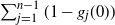 $\sum_{j=1}^{n-1}(1-g_j(0))$
. This completes the proof of (25) in the general case.
$\sum_{j=1}^{n-1}(1-g_j(0))$
. This completes the proof of (25) in the general case.
Equality (25) implies that
 \begin{align*}F(n)\sim \dfrac{1}{n^{\gamma}L(n)},\end{align*}
where
 \begin{align*}L(n) = C^{-1}_{1}\exp\Biggl\{-\sum_{j=1}^{n-1} (1-f_{j}(0) )^{2} \sum_{l=0}^{\infty}f_{j}^{l}(0) \sum_{i=l+1}^{\infty}R_{i}\Biggr\}\quad\text{and}\quad C_1\gt 0.\end{align*}
It is now obvious that (21) is equivalent to
 \begin{equation}\lim_{n\to\infty}\sum_{j=1}^{n-1} (1-f_{j}(0) )^{2} \sum_{l=0}^{\infty}f_{j}^{l}(0) \sum_{i=l+1}^{\infty}R_{i} = \infty.\end{equation}
Set $\overline{R}_{l}\,:\!=\, \sum_{i=l+1}^{\infty}R_{i}$
. It follows from (18) that
$\overline{R}_{l}\,:\!=\, \sum_{i=l+1}^{\infty}R_{i}$
. It follows from (18) that $f_j^l(0)\ge c_0$
for all
$f_j^l(0)\ge c_0$
for all $1\le l\le j$
and
$1\le l\le j$
and $(1-f_j(0))^2\ge c_1 j^{-2}$
for all
$(1-f_j(0))^2\ge c_1 j^{-2}$
for all $j\ge1$
. Using these estimates and interchanging the order of summation, we get
$j\ge1$
. Using these estimates and interchanging the order of summation, we get
 \begin{align*} \sum_{j=1}^{n-1} (1-f_{j}(0) )^{2} \sum_{l=0}^{\infty}f_{j}^{l}(0) \sum_{i=l+1}^{\infty}R_{i}&=\sum_{i=1}^{n-1} (1-f_{j}(0) )^{2} \sum_{l=0}^{\infty}f_{j}^{l}(0)\overline{R}_{l}\\&\geq c_1^{2} \sum_{j=1}^{n-1}\dfrac{1}{j^{2}}\sum_{l=1}^{j}c_0\overline{R}_{l}\\&\ge c_{2} \sum_{l=1}^{n/2} \overline{R}_{l} \sum_{j=l}^{n-1}\dfrac{1}{j^{2}} \\&\geq \dfrac{c_{2}}{4} \sum_{l=1}^{n/2} \overline{R_{l}} \dfrac{1}{l}\\&\ge\dfrac{c_{2}}{4} \sum_{l=1}^{n/2}\dfrac{1}{l}\sum_{i=l+1}^{n/2} R_{i} \\&= \dfrac{c_{2}}{4} \sum_{i=2}^{n/2 } R_{i} \sum_{l=1}^{i-1}\dfrac{1}{l}\\& \geq c_{3} \sum_{i=2}^{n/2} R_{i}\log i\to \infty \quad\text{as $n\to\infty$,}\end{align*}
where in the last step we used the assumption $\sum_{k=1}^{\infty} (k \log k )q_{k}= \infty$
. This proves (26) and thus (21).
$\sum_{k=1}^{\infty} (k \log k )q_{k}= \infty$
. This proves (26) and thus (21).
Lemma 5. Assume that (3) holds. If
 \begin{align*}\sum_{k=1}^\infty (k^{2}\log k ) p_{k}=\infty\quad and \quad\sum_{k=1}^\infty (k\log k ) q_{k}\lt\infty,\end{align*}
then
 \begin{equation} L(n) \to +\infty \quad as\ n\to \infty.\end{equation}
Proof. Changing the order of summation, we have
 \begin{align*}\sum_{j=1}^{\infty} (1-f_{j}(0) )^{2} \sum_{l=0}^{\infty}f_{j}^{l}(0) \sum_{i=l+1}^{\infty}R_{i}&=\sum_{j=1}^{\infty} (1-f_{j}(0) )^{2}\sum_{i=1}^\infty R_i\sum_{l=0}^{i-1}f_{j}^{l}(0)\\&=\sum_{j=1}^{\infty} (1-f_{j}(0) )\sum_{i=1}^\infty R_i\big[1-f_j^i(0)\big]\\&=\sum_{i=1}^\infty R_i\sum_{j=1}^\infty (1-f_{j}(0) )\big[1-f_j^i(0)\big].\end{align*}
Using bounds $1-f_{j}(0)\le {{C}/{j}}$
and
$1-f_{j}(0)\le {{C}/{j}}$
and $1-f_j^i(0)\le i(1-f_j(0))$
, we obtain
$1-f_j^i(0)\le i(1-f_j(0))$
, we obtain
 \begin{align*} \sum_{j=1}^\infty (1-f_{j}(0) )\big[1-f_j^i(0)\big]&\le \sum_{j=1}^i (1-f_{j}(0) )+\sum_{j=i+1}^\infty i (1-f_{j}(0) )^2\\&\le \sum_{j=1}^i\dfrac{C}{j}+\sum_{j=i+1}^\infty\dfrac{C^2i}{j^2}\\&\le C_1\log i,\quad i\ge2.\end{align*}
Then, according to the assumption $\sum_{k\ge 1} (k\log k )q_{k}\lt\infty$
,
$\sum_{k\ge 1} (k\log k )q_{k}\lt\infty$
,
 \begin{align*} \sum_{j=1}^{\infty} (1-f_{j}(0) )^{2} \sum_{l=0}^{\infty}f_{j}^{l}(0) \sum_{i=l+1}^{\infty}R_{i}\lt\infty.\end{align*}
Combining this with (23) and with (24), we establish
 \begin{align}F(n)\sim C_{2} \exp\Biggl\{-h'(1)\sum_{j=1}^{n-1} (1-f_{j}(0) )\Biggr\}\quad\text{as $ n\to\infty$.}\end{align}
Following [Reference Nagaev and Vakhtel6], we define
 \begin{align*}u(s)=\dfrac{1}{1-f(s)}-\dfrac{1}{1-s}.\end{align*}
We also define
 \begin{align*}\delta(s)=\dfrac{B}{2}-u(s).\end{align*}
Then we have
 \begin{align}\nonumber\dfrac{1}{1-f_n(0)}-1&=\sum_{k=0}^{n-1}\biggl(\dfrac{1}{1-f_{k+1}(0)}-\dfrac{1}{1-f_{k}(0)}\biggr)\\&=\sum_{k=0}^{n-1}u(f_k(0)) \notag \\&=\dfrac{Bn}{2}-\sum_{k=0}^{n-1}\delta(f_k(0)).\end{align}
Thus
 \begin{align*} 1-f_{n}(0)=\Biggl(1+\dfrac{Bn}{2}-\sum_{k=0}^{n-1}\delta (f_{k}(0) ) \Biggr)^{-1}. \end{align*}
Let $\varepsilon(s)$
be such that
$\varepsilon(s)$
be such that
 \begin{align*}f(s)=s+\biggl(\dfrac{B}{2}-\varepsilon(s)\biggr)(1-s)^2.\end{align*}
To derive an explicit expression for $\varepsilon(s)$
, we first expand
$\varepsilon(s)$
, we first expand $f(s)-s$
by using the definition of f(s):
$f(s)-s$
by using the definition of f(s):
 \begin{align*} f(s)-s=p_0(1-s)+\sum_{w=2}^{\infty}p_{w}(s^{w}-s)=p_0(1-s)-(1-s)\sum_{w=2}^{\infty}p_{w}\sum_{j=1}^{w-1}s^{j}. \end{align*}
Next, using the identity
 \begin{align*} s^{j}=1-j(1-s)+(1-s)\sum_{v=1}^{j-1}(1-s^{v})\end{align*}
and the criticality assumption $f'(1)=\sum_{w=1}^\infty wp_w=1$
, we get
$f'(1)=\sum_{w=1}^\infty wp_w=1$
, we get
 \begin{align*}f(s)-s&=p_0(1-s)-(1-s)\sum_{w=2}^{\infty}p_{w}\sum_{j=1}^{w-1}\Biggl(1-j(1-s)+(1-s)\sum_{v=1}^{j-1}(1-s^{v}) \Biggr) \\& =(1-s)\Biggl(p_0-\sum_{w=2}^\infty(w-1)p_w\Biggr)+(1-s)^{2}\sum_{w=2}^{\infty}p_{w}\sum_{j=1}^{w-1}\Biggl(j-\sum_{v=1}^{j-1} (1-s^{v} )\Biggr)\\&=(1-s)^2\sum_{w=2}^\infty p_w\dfrac{w(w-1)}{2}-(1-s)^2\sum_{w=3}^{\infty}p_{w}\sum_{j=2}^{w-1}\sum_{v=1}^{j-1} (1-s^{v} ).\end{align*}
Noting that
 \begin{align*}\sum_{w=2}^\infty\frac{w(w-1)}{2}p_w=\frac{B}{2},\end{align*}
we finally conclude that
 \begin{equation}\varepsilon (s )=\sum_{w=3}^{\infty}p_{w}\sum_{j=2}^{w-1}\sum_{v=1}^{j-1} (1-s^{v} ), \quad |s| \le 1.\end{equation}
It is also clear that $\varepsilon(s)\in[0,{{B}/{2}}]$
for
$\varepsilon(s)\in[0,{{B}/{2}}]$
for $s\in[0, 1]$
.
$s\in[0, 1]$
.
We next notice that
 \begin{align*}\delta(s)&=\dfrac{B}{2}-u(s)\\&=\dfrac{B}{2}-\biggl(\dfrac{1}{1-f(s)}-\dfrac{1}{1-s}\biggr)\\&=\dfrac{B}{2}-\dfrac{f(s)-s}{(1-s)(1-f(s))}\\&=\dfrac{B}{2}-\dfrac{{{B}/{2}}-\varepsilon(s)}{1-(1-s)({{B}/{2}}-\varepsilon(s))}\\&=\dfrac{\varepsilon(s)-\frac{B}{2}(1-s)({{B}/{2}}-\varepsilon(s))}{1-(1-s)({{B}/{2}}-\varepsilon(s))}\\&=\!:\, \varepsilon(s)+\gamma(s)\end{align*}
and $\gamma(s)={\mathrm{O}} ((1-s))$
as
$\gamma(s)={\mathrm{O}} ((1-s))$
as $s\to 1$
. Plugging this representation of
$s\to 1$
. Plugging this representation of $\delta(s)$
into (29), we obtain
$\delta(s)$
into (29), we obtain
 \begin{align*}\dfrac{1}{1-f_n(0)}=1+\dfrac{Bn}{2}-\sum_{k=0}^{n-1}\varepsilon(f_k(0))-\sum_{k=0}^{n-1}\gamma(f_k(0)).\end{align*}
Combining $\gamma(s)={\mathrm{O}} ((1-s))$
and (18), we obtain
$\gamma(s)={\mathrm{O}} ((1-s))$
and (18), we obtain
 \begin{align*}\sum_{k=0}^{n-1}\gamma(f_k(0))={\mathrm{O}} ({\log}\ n), \quad n\to \infty.\end{align*}
Noting that $\varepsilon(f_k(0))\to0$
as
$\varepsilon(f_k(0))\to0$
as $k\to\infty$
, we infer that
$k\to\infty$
, we infer that $\sum_{k=0}^{n-1}\varepsilon(f_k(0))={\mathrm{o}} (n)$
. Combining this with the equality
$\sum_{k=0}^{n-1}\varepsilon(f_k(0))={\mathrm{o}} (n)$
. Combining this with the equality
 \begin{align*}\dfrac{1}{a_n+b_n}=\dfrac{1}{a_n}+{\mathrm{O}} \biggl(\dfrac{b_n}{a_n^2}\biggr),\quad n\to \infty,\end{align*}
which is valid for all sequences $\{a_n\}$
,
$\{a_n\}$
, $\{b_n\}$
satisfying
$\{b_n\}$
satisfying $a_n\to\infty$
and
$a_n\to\infty$
and $b_n={\mathrm{o}} (a_n)$
, we conclude that
$b_n={\mathrm{o}} (a_n)$
, we conclude that
 \begin{align*}1-f_n(0)=\Biggl(1+\dfrac{Bn}{2}-\sum_{k=0}^{n-1}\varepsilon(f_k(0))\Biggr)^{-1}+{\mathrm{O}} \biggl(\dfrac{\log n}{n^2}\biggr), \quad n\to \infty.\end{align*}
Plugging this into (28), we obtain
 \begin{align}F(n)\sim C_{3} \exp\Biggl\{-h'(1)\sum_{j=1}^{n-1}\Biggl(1+\dfrac{Bj}{2}-\sum_{k=0}^{j-1}\varepsilon(f_k(0))\Biggr)^{-1}\Biggr\},\quad n\to\infty.\end{align}
Thus it suffices to analyse the asymptotic behaviour of the sum
 \begin{align*}h^{\prime}(1)\sum_{j=1}^{n-1}\Biggl(1+\dfrac{Bj}{2}-\sum_{k=0}^{j-1}\varepsilon(f_k(0))\Biggr)^{-1}.\end{align*}
Since $\varepsilon(s)$
is non-negative on the interval [0, 1], applying the inequality
$\varepsilon(s)$
is non-negative on the interval [0, 1], applying the inequality
 \begin{align*}\dfrac{1}{a-b}\ge \dfrac{1}{a}+\dfrac{b}{a^2},\quad 0\le b\le a,\end{align*}
we obtain
 \begin{align*}\Biggl(1+\dfrac{Bj}{2}-\sum_{k=0}^{j-1}\varepsilon(f_k(0))\Biggr)^{-1}\ge \biggl(1+\frac{Bj}{2}\biggr)^{-1}+\biggl(1+\frac{Bj}{2}\biggr)^{-2}\sum_{k=0}^{j-1}\varepsilon(f_k(0)).\end{align*}
Consequently
 \begin{align*}&h'(1)\sum_{j=1}^{n-1}\Biggl(1+\dfrac{Bj}{2}-\sum_{k=0}^{j-1}\varepsilon(f_k(0))\Biggr)^{-1}\\&\quad \ge h'(1)\sum_{j=1}^{n-1}\biggl(1+\dfrac{Bj}{2} \biggr)^{-1}+\sum_{j=1}^{n-1}\dfrac{1}{(1+{{Bj}/{2}} )^{2}}\sum_{k=0}^{j-1}\varepsilon (f_{k}(0) )\\&\quad \ge \gamma\log n-c_1+c_2\sum_{j=1}^{n-1}\dfrac{1}{j^{2}}\sum_{k=0}^{j-1}\varepsilon (f_{k}(0) ).\end{align*}
Combining this with (31), we see that the convergence $L(n)\to \infty$
will be proved if we show that the latter sum grows unboundedly. To this end, we first notice that
$L(n)\to \infty$
will be proved if we show that the latter sum grows unboundedly. To this end, we first notice that
 \begin{align*}\sum_{j=1}^{n-1}\dfrac{1}{j^{2}}\sum_{k=0}^{j-1}\varepsilon (f_{k}(0) )= \sum_{k=0}^{n-2}\varepsilon (f_{k}(0) )\sum_{j=k+1}^{n-1}\dfrac{1}{j^{2}}\geq \dfrac{n/2-1}{2n}\sum_{k=1}^{n/2}\dfrac{1}{k}\varepsilon (f_{k}(0) ),\end{align*}
where in the last step we used the inequalities
 \begin{align*}\sum_{j=k+1}^{n-1}\dfrac{1}{j^2}\ge \int_{k+1}^{n}\dfrac{{\mathrm{d}} x}{x^2}=\dfrac{1}{k+1}-\dfrac{1}{n}\ge\dfrac{n/2-1}{2nk},\quad 1\le k\le n/2.\end{align*}
Thus we need to show that
 \begin{equation}\sum_{k=1}^{\infty}\dfrac{\varepsilon (f_{k}(0) )}{k} = \infty.\end{equation}
Changing the order of summation in (30), we have
 \begin{align*}\varepsilon (f_{k}(0) )& = \sum_{u=3}^{\infty}p_{u}\sum_{j=2}^{u-1}\sum_{v=1}^{j-1} \big(1-f_{k}^{v}(0) \big) \\& =\sum_{j=2}^{\infty}\sum_{u=j+1}^{\infty}p_{u}\sum_{v=1}^{j-1} \big(1-f_{k}^{v}(0) \big)\\& =\sum_{j=2}^{\infty}K_{j}\sum_{v=1}^{j-1} \big(1-f_{k}^{v}(0) \big),\end{align*}
where $K_{j}=\sum_{u=j+1}^{\infty}p_{u}$
. Interchanging the order of the remaining two sums, we finally get
$K_{j}=\sum_{u=j+1}^{\infty}p_{u}$
. Interchanging the order of the remaining two sums, we finally get
 \begin{align*}\varepsilon (f_{k}(0) )=\sum_{v=1}^{\infty} \big(1-f_{k}^{v}(0) \big)\sum_{j=v+1}^{\infty}K_{j}= \sum_{v=1}^{\infty} \big(1-f_{k}^{v}(0) \big)\overline{K_{v}},\end{align*}
where $\overline{K_{v}}=\sum_{j=v+1}^{\infty}K_{j}$
. This representation implies that
$\overline{K_{v}}=\sum_{j=v+1}^{\infty}K_{j}$
. This representation implies that
 \begin{align*} \sum_{k=1}^\infty\dfrac{1}{k}\varepsilon (f_{k}(0) )& = \sum_{k=1}^\infty\dfrac{1}{k}\sum_{v=1}^{\infty}\overline{K_{v}} \big(1-f_{k}^{v}(0) \big) \\&= \sum_{v=1}^{\infty}\overline{K_{v}}\sum_{k=1}^{\infty}\dfrac{1}{k} \big(1-f_{k}^{v}(0) \big)\\&\ge\sum_{v=1}^{\infty} \overline{K_{v}}\sum_{k=1}^{v}\dfrac{1-f_{k}^{v}(0)}{k}.\end{align*}
Noting that $f_{k}(0)$
is increasing in k and using (18), we obtain
$f_{k}(0)$
is increasing in k and using (18), we obtain
 \begin{align*}\sum_{k=1}^{v}\dfrac{1-f_{k}^{v}(0)}{k}\ge \big(1-f_{v}^{v}(0) \big)\sum_{k=1}^{v}\dfrac{1}{k}\ge c\log v.\end{align*}
Therefore
 \begin{align*}\sum_{k=1}^\infty\dfrac{1}{k}\varepsilon (f_{k}(0) )\ge c \sum_{v=1}^{\infty} \overline{K_{v}}\log v.\end{align*}
Now it remains to notice that the assumption $\sum_{k=1}^{\infty} (k^{2}\log k )p_{k}=\infty$
is equivalent to
$\sum_{k=1}^{\infty} (k^{2}\log k )p_{k}=\infty$
is equivalent to
 \begin{align*}\sum_{v=1}^{\infty} \overline{K_{v}}\log v=\infty.\end{align*}
This concludes the proof of (32), which, in turn, implies (27).
To investigate the asymptotic behaviour of lower deviations for $Y_{n}$
, we need the following lemma, which deals with lower and upper bounds for
$Y_{n}$
, we need the following lemma, which deals with lower and upper bounds for $\mathbb P (Y_{n}\leq k )$
. Recall that in this section we always assume that
$\mathbb P (Y_{n}\leq k )$
. Recall that in this section we always assume that $Y_0=0$
.
$Y_0=0$
.
Lemma 6. There exist positive constants $c_{1}$
and
$c_{1}$
and $c_{2}$
such that
$c_{2}$
such that
 \begin{equation}\mathbb P (Y_{n} \leq k )\geq c_{1}\prod_{j=k}^{n-1}h (f_{j}(0) ),\quad k_0\leq k\leq n\end{equation}
and
 \begin{equation}\mathbb P (Y_{n} \leq k )\leq c_{2}\prod_{j=k}^{n-1}h (f_{j}(0) ),\quad 1\le k\le n,\end{equation}
where $k_0=\min\{k\ge0\,\colon q_k\gt 0\}\vee1$
.
$k_0=\min\{k\ge0\,\colon q_k\gt 0\}\vee1$
.
Proof. We first prove (34). By the Markov inequality,
 \begin{align*}\mathbb P (Y_{n} \leq k )=\mathbb P \big(s^{Y_{n}} \geq s^{k} \big)\leq \dfrac{H_{n} (s )}{s^{k}},\quad s\in(0,1).\end{align*}
Letting $s=f_{k}(0)$
, we get
$s=f_{k}(0)$
, we get
 \begin{align*}\mathbb P (Y_{n} \leq k ) \leq \dfrac{H_{n} (f_{k}(0) )}{ (f_{k}(0) )^{k}}.\end{align*}
Notice that (18) implies that $ (f_{k}(0) )^{k}\ge c_{3}\gt 0$
for all
$ (f_{k}(0) )^{k}\ge c_{3}\gt 0$
for all $k\geq 0 $
. Therefore
$k\geq 0 $
. Therefore
 \begin{align*}\mathbb P (Y_{n} \leq k ) \leq \dfrac{H_{n} (f_{k}(0) )}{c_3}.\end{align*}
Observe that
 \begin{equation*} H_{n} (f_{k}(0) )= \prod_{j=0}^{n-1} h (f_{j} (f_{k}(0) ) )=\prod_{j=k}^{n+k-1} h (f_{j}(0) ).\end{equation*}
To complete the proof of (34), it remains to notice that
 \begin{equation*}\prod_{j=k}^{n+k-1} h (f_{j}(0) )\le \prod_{j=k}^{n-1} h (f_{j}(0) ).\end{equation*}
To prove (33), we notice that if all immigrants from the first $n-k$
generations have no descendants at time n, then
$n-k$
generations have no descendants at time n, then $Y_{n}$
has the same distribution as
$Y_{n}$
has the same distribution as $Y_{k}$
. Therefore
$Y_{k}$
. Therefore
 \begin{align*}\mathbb P (Y_{n} \leq k ) \geq\mathbb P (Y_{k} \leq k )\prod_{i=1}^{n-k}\mathbb P \bigl(Z_{n-i}^{ (i )}=0 \bigr).\end{align*}
Due to the limit theorem (4), there exists a positive number c such that
 \begin{align*} \mathbb P (Y_{k} \leq k )\geq c\gt 0 \end{align*}
uniformly in $k\ge k_0\,:\!=\, \min\{j\ge0\,\colon q_j\gt 0\}\vee1$
. Furthermore, it is immediate from the definition of processes
$k\ge k_0\,:\!=\, \min\{j\ge0\,\colon q_j\gt 0\}\vee1$
. Furthermore, it is immediate from the definition of processes $Z_{n-i}^{ (i )}$
that
$Z_{n-i}^{ (i )}$
that
 \begin{align*}\prod_{i=1}^{n-k}\mathbb P \bigl(Z_{n-i}^{ (i )}=0 \bigr)= \prod_{j=k}^{n-1} h (f_{j}(0) ).\end{align*}
Thus the lower bound is also proved.
3. Estimates for concentration functions
The aim of this section is to provide some estimates for local probabilities of random variables $Y_{n}$
and
$Y_{n}$
and $Z^{(i)}_{n-i}$
, which will be used in the proof of local asymptotics (8) and (9). Since these two statements use the aperiodicity condition on the distributions
$Z^{(i)}_{n-i}$
, which will be used in the proof of local asymptotics (8) and (9). Since these two statements use the aperiodicity condition on the distributions $\{p_k\}$
and
$\{p_k\}$
and $\{q_k\}$
, we shall always assume in the present section that this condition holds.
$\{q_k\}$
, we shall always assume in the present section that this condition holds.
We begin with bounds for the concentration function of $Y_n$
.
$Y_n$
.
Lemma 7. For every $\varepsilon\gt 0$
, there exists
$\varepsilon\gt 0$
, there exists $N=N (\varepsilon )$
such that for all
$N=N (\varepsilon )$
such that for all $n\gt N$
and
$n\gt N$
and $ |s |\leq 1$
,
$ |s |\leq 1$
,
 \begin{align*}\biggl|\dfrac{H_{n} (s )}{h(s)}\biggr| \leq \exp \Biggl\{- (h'(1)-B\varepsilon ) \sum_{j=N}^{n-1} \,\mathrm{Re} (1-f_{j} (s ) )+\varepsilon \sum_{j=N}^{n-1} |\mathrm{Im} (1-f_{j}(s) ) | \Biggr\} .\end{align*}
Proof. The proof is the same as the proof of Lemma 6 in [Reference Nagaev and Vakhtel6]. For readers’ convenience and completeness, we provide the proof below.
Since $|h (f_{j} (s ) )| \leq 1$
, we obtain for all
$|h (f_{j} (s ) )| \leq 1$
, we obtain for all $n\gt N\ge1$
the inequality
$n\gt N\ge1$
the inequality
 \begin{equation}\biggl|\dfrac{H_{n} (s )}{h(s)}\biggr|=\Biggl|\prod_{j=1}^{n-1}h (f_{j} (s ) ) \Biggr|\leq \Biggl|\prod_{j=N}^{n-1}h (f_{j} (s ) ) \Biggr|= \exp\Biggl\{\sum_{j=N}^{n-1} \,\mathrm{Re} \log h (f_{j} (s ) )\Biggr\}.\end{equation}
In view of (17), for $ |s |\leq 1$
, we have
$ |s |\leq 1$
, we have
 \begin{align}\mathrm{Re}\log h (f_{j} (s ) )& \leq - (h'(1)- |\mathrm{Re}\,\alpha (f_{j} (s ) ) | )\,\mathrm{Re} (1-f_{j} (s ) ) + |\mathrm{Im}\,\alpha (f_{j} (s ) ) |\, |\mathrm{Im} (1-f_{j} (s ) ) |.\end{align}
It is immediate from the triangle inequality that
 \begin{align*}|1-f_j(s)|\le \sum_{k=1}^\infty\mathbb P(Z_j=k)|1-s^k|\le 2\mathbb P(Z_j\gt 0).\end{align*}
This implies that $f_{j} (s )\to 1$
as
$f_{j} (s )\to 1$
as $j\to\infty$
uniformly in s from the unity disk. Thus one can choose
$j\to\infty$
uniformly in s from the unity disk. Thus one can choose $N=N (\varepsilon )$
such that for all
$N=N (\varepsilon )$
such that for all $j \geq N$
,
$j \geq N$
,
 \begin{align*} |\mathrm{Re}\ \alpha (f_{j} (s ) ) | \leq \varepsilon B, \quad |\mathrm{Im}\ \alpha (f_{j} (s ) ) |\leq \varepsilon.\end{align*}
Substituting the above bounds into (36) and recalling (35), we arrive at the conclusion of the lemma.
Lemma 8. For each $\varepsilon \in (0,2\gamma)$
there exists a number
$\varepsilon \in (0,2\gamma)$
there exists a number $A(\varepsilon)\gt 0$
such that, for any
$A(\varepsilon)\gt 0$
such that, for any $n \geq 1$
and
$n \geq 1$
and $ |t | \leq \pi / 2$
,
$ |t | \leq \pi / 2$
,
 \begin{align*} |H_n ({\mathrm{e}}^{\mathrm{i}t} ) | \leq\biggl|\dfrac{H_n ({\mathrm{e}}^{\mathrm{i}t} )}{h({\mathrm{e}}^{\mathrm{i}t})}\biggr| \leq A(\varepsilon) (n|t| )^{-2 ( (\gamma-2\varepsilon ) (1-\varepsilon )-{{2\varepsilon^{2}}/{B}} )}.\end{align*}
In particular, there exists a constant $c^{*}$
such that, for every
$c^{*}$
such that, for every $n\ge1$
and all
$n\ge1$
and all $\frac{1}{n}\le |t | \leq \pi / 2$
,
$\frac{1}{n}\le |t | \leq \pi / 2$
,
 \begin{align*} |H_n ({\mathrm{e}}^{\mathrm{i}t} ) |\leq\biggl|\dfrac{H_n ({\mathrm{e}}^{\mathrm{i}t} )}{h({\mathrm{e}}^{\mathrm{i}t})}\biggr|\leq c^* (n|t| )^{-\theta},\end{align*}
where $\theta=\min\{\gamma,1/2\}$
.
$\theta=\min\{\gamma,1/2\}$
.
Proof. Consider the function
 \begin{align*} \psi(x)=\dfrac{2 (Bx/2+1 )}{ (Bx/2+1 )^{2}+c^{2}}, \quad x \geq 0. \end{align*}
It is immediate from Lemma 7 in [Reference Nagaev and Vakhtel6] that
 \begin{equation}\Biggl|\sum_{k=0}^{n-1}\psi(k)-\dfrac{2}{B}\log\biggl(1+\dfrac{ (Bn/2+1 )^{2}}{c^{2}} \biggr) \Biggr| \leq 1.\end{equation}
Further, by Lemma 8 in [Reference Nagaev and Vakhtel6], there exist N and constants $a=a (\varepsilon,N )$
and
$a=a (\varepsilon,N )$
and $b=b (\varepsilon,N )$
such that for all
$b=b (\varepsilon,N )$
such that for all $ |t |\leq \pi/2$
,
$ |t |\leq \pi/2$
,
 \begin{align}\sum_{j=N}^{n-1}\,\mathrm{Re} \big(1-f_{j} ({\mathrm{e}}^{\mathrm{i}t} ) \big)&\geq \dfrac{2 (1-\varepsilon )}{B}\log \biggl(1+ (Bn/2+1 )^{2}\tan^{2}\dfrac{t}{2} \biggr)-a,\end{align}
 \begin{align}\sum_{j=N}^{n-1} |\mathrm{Im} \big(1-f_{j} ({\mathrm{e}}^{\mathrm{i}t} ) \big) | &\leq \dfrac{2\varepsilon}{B}\log \biggl(1+ (Bn/2+1 )^{2}\tan^{2}\dfrac{t}{2} \biggr)+b.\end{align}
Using Lemma 8 and applying then (37)–(39) and $ |x |\leq |\tan x |$
, we conclude that
$ |x |\leq |\tan x |$
, we conclude that
 \begin{align*}\biggl|\dfrac{H_{n} ({\mathrm{e}}^{\mathrm{i}t} )}{h({\mathrm{e}}^{\mathrm{i}t})}\biggr|&\leq A_1 (\varepsilon )\exp \biggl\{ \biggl(-(\gamma-2\varepsilon)(1-\varepsilon)+\dfrac{2\varepsilon^2}{B} \biggr)\log \biggl(1+ (Bn/2+1 )^{2}\tan^{2}\dfrac{t}{2} \biggr) \biggr\}\\&\le A_2(\varepsilon) (n^2\tan^2(t/2) )^{- ( (\gamma-2\varepsilon ) (1-\varepsilon )-{{2\varepsilon^{2}}/{B}} )}\\&\leq A_3 (\varepsilon ) (n |t | )^{-2 ( (\gamma-2\varepsilon ) (1-\varepsilon )-{{2\varepsilon^{2}}/{B}} )},\end{align*}
where $A_1(\varepsilon)$
,
$A_1(\varepsilon)$
, $A_2(\varepsilon)$
, and
$A_2(\varepsilon)$
, and $A_3(\varepsilon)$
are finite positive numbers. This gives the first estimate. Choosing
$A_3(\varepsilon)$
are finite positive numbers. This gives the first estimate. Choosing $\varepsilon$
so small that
$\varepsilon$
so small that
 \begin{align*}2 \biggl( (\gamma-2\varepsilon ) (1-\varepsilon )-\frac{2\varepsilon^{2}}{B} \biggr)\ge \theta\end{align*}
and using the restriction $n|t|\ge 1$
, we obtain the second estimate.
$n|t|\ge 1$
, we obtain the second estimate.
Lemma 9. There exists a constant c such that for all $n,m \geq 1$
,
$n,m \geq 1$
,
 \begin{align*}\mathbb P (Y_{n}=m ) \leq \dfrac{c}{m}.\end{align*}
Proof. We make use of the following bound for the concentration function (see e.g. the proof of Lemma 4 in [Reference Nagaev and Vakhtel6]):
 \begin{equation}\sup_{x}\mathbb P (\xi = x ) \leq \biggl(\dfrac{96}{95}\biggr)^{2}\dfrac{1}{a}\int_{-a}^{a} |\varphi (t ) |\,{\mathrm{d}} t,\end{equation}
where $\varphi (t )$
is the characteristic function of the random variable
$\varphi (t )$
is the characteristic function of the random variable $\xi$
, and
$\xi$
, and $a\gt 0$
.
$a\gt 0$
.
Now let $\xi$
be a random variable with the generating function
$\xi$
be a random variable with the generating function $H_{n}^{\prime} (s ) / H_{n}^{\prime}(1)$
. Then, for any
$H_{n}^{\prime} (s ) / H_{n}^{\prime}(1)$
. Then, for any $n \geq 1$
,
$n \geq 1$
,
 \begin{equation}\sup_{k} k \mathbb P (Y_{n}=k )\leq\biggl(\dfrac{96}{95}\biggr)^{2}\dfrac{1}{a}\int_{-a}^{a} |H_{n}^{\prime} (\mathrm{e}^{\mathrm{i} t} ) |\,{\mathrm{d}} t.\end{equation}
Observe that for $|s|\le 1$
, we have
$|s|\le 1$
, we have
 \begin{align*}H_{n}^{\prime} (s )=\sum_{j=0}^{n-1} h^{\prime} (f_{j} (s ) ) f_{j}^{\prime} (s ) \prod_{0\le l\le n-1,\ l\neq j} h (f_{l} (s ) ) = H_{n} (s )\sum_{l=0}^{n-1}\dfrac{h^{\prime} (f_{l} (s ) )}{h (f_{l} (s ) )} f_{l}^{\prime} (s ).\end{align*}
We shall estimate integrals of
 \begin{align*} \biggl|H_{n}({\mathrm{e}}^{\mathrm{i}t})\dfrac{h^{\prime} \big(f_{l} ({\mathrm{e}}^{\mathrm{i}t} ) \big)}{h \big(f_{l} ({\mathrm{e}}^{\mathrm{i}t} ) \big)} f_{l}^{\prime} ({\mathrm{e}}^{\mathrm{i}t} ) \biggr|\end{align*}
separately. If $l=0$
, then
$l=0$
, then $f_{l}'(s)\equiv 1$
and the function
$f_{l}'(s)\equiv 1$
and the function $h'(f_{l}({\mathrm{e}}^{\mathrm{i}t}))$
is bounded. Noting that
$h'(f_{l}({\mathrm{e}}^{\mathrm{i}t}))$
is bounded. Noting that
 \begin{align*} \biggl|\frac{H_{n} ({\mathrm{e}}^{\mathrm{i}t} )}{h({\mathrm{e}}^{\mathrm{i}t})} \biggr|\end{align*}
is bounded as well, we get
 \begin{align}\int_{1/n\lt|t|\lt a} \biggl|H_{n} ({\mathrm{e}}^{\mathrm{i}t} )\dfrac{h^{\prime} ({\mathrm{e}}^{\mathrm{i}t} )}{h ({\mathrm{e}}^{\mathrm{i}t} )} \biggr|\,{\mathrm{d}} t\le C.\end{align}
Assume now that $l\ge1$
. As we have noticed before,
$l\ge1$
. As we have noticed before, $\ f_l(s)\to1$
as
$\ f_l(s)\to1$
as $l\to\infty$
uniformly in
$l\to\infty$
uniformly in $|s|\le1$
. This property allows us to conclude that if a is sufficiently small then
$|s|\le1$
. This property allows us to conclude that if a is sufficiently small then
 \begin{align*} |h \big(f_l ({\mathrm{e}}^{\mathrm{i}t} ) \big) |\ge\dfrac{1}{2}\quad\text{for all }l\ge1\text{ and all }t\in[-a,a].\end{align*}
Combining this with the bounds $ |f'_{l} ({\mathrm{e}}^{\mathrm{i}t} ) | \leq 1$
,
$ |f'_{l} ({\mathrm{e}}^{\mathrm{i}t} ) | \leq 1$
, $ |h^{\prime} \big(f_{l} ({\mathrm{e}}^{\mathrm{i}t} ) \big) |\le h'(1)$
and applying Lemma 8, we obtain
$ |h^{\prime} \big(f_{l} ({\mathrm{e}}^{\mathrm{i}t} ) \big) |\le h'(1)$
and applying Lemma 8, we obtain
 \begin{align}\int_{1 / n\lt|t|\lt \min\{1 / l,a\}} \biggl|H_{n} ({\mathrm{e}}^{\mathrm{i}t} )\dfrac{h^{\prime} \big(f_{l} ({\mathrm{e}}^{\mathrm{i}t} ) \big)}{h \big(f_{l} ({\mathrm{e}}^{\mathrm{i}t} ) \big)} f_{l}^{\prime} ({\mathrm{e}}^{\mathrm{i}t} ) \biggr|\,{\mathrm{d}} t\leq c^*\int_{1/n\lt|t|\lt 1/l} (n|t| )^{-\theta}\,{\mathrm{d}} t\leq \dfrac{c^*}{1-\theta}\dfrac{l^{\theta-1}}{n^{\theta}}.\end{align}
For $|t|\ge1/l$
, we additionally use the inequality
$|t|\ge1/l$
, we additionally use the inequality
 \begin{align*} |f'_{l} ({\mathrm{e}}^{\mathrm{i}t} ) | \leq \dfrac{c}{ (l |t | )^{3/2}},\end{align*}
which was derived in the proof of Lemma 9 from [Reference Nagaev and Vakhtel6]. As a result, we have
 \begin{align}\nonumber&\int_{\min\{1 / l,a\}\lt|t|\lt a} \biggl|H_{n} ({\mathrm{e}}^{\mathrm{i}t} )\dfrac{h^{\prime} \big(f_{l} ({\mathrm{e}}^{\mathrm{i}t} ) \big)}{h \big(f_{l} ({\mathrm{e}}^{\mathrm{i}t} ) \big)} f_{l}^{\prime} ({\mathrm{e}}^{\mathrm{i}t} ) \biggr|\,{\mathrm{d}} t \\&\quad\leq c_1\int_{\min\{1 / l,a\}\lt|t|\lt a}(n|t|)^{-\theta}(l|t|)^{-3/2}\,{\mathrm{d}} t \notag \\&\quad\leq c_2\dfrac{l^{\theta-1}}{n^{\theta}}.\end{align}
Summing over l the estimates in (43) and (44) and taking into account (42), we obtain
 \begin{align*}\int_{1/n\lt|t|\lt a} |H'_n({\mathrm{e}}^{\mathrm{i}t}) |\,{\mathrm{d}} t\le c.\end{align*}
Using the elementary bound
 \begin{align*} |H'_{n} ({\mathrm{e}}^{\mathrm{i}t} ) |\le h'(1)n,\end{align*}
we get
 \begin{align*}\int_{|t|\lt1/n} |H'_{n} ({\mathrm{e}}^{\mathrm{i}t} ) |\,{\mathrm{d}} t\le 2h'(1).\end{align*}
Consequently
 \begin{align*}\int_{-a}^{a} |H_{n}^{\prime} (\mathrm{e}^{\mathrm{i} t} ) |\,{\mathrm{d}} t\le c.\end{align*}
Plugging this into (41), we complete the proof of the lemma.
For the proof of our main result, we also need a concentration function bound for the Galton–Watson process $\{Z^{(l)}_n\}$
, which starts with a random number of particles.
$\{Z^{(l)}_n\}$
, which starts with a random number of particles.
Lemma 10. There exists a constant c such that for all $1\le l \lt n$
we have
$1\le l \lt n$
we have
 \begin{align*}\mathbb P \bigl(Z^{(l)}_{n-l}\gt 0 \bigr)\le \dfrac{c}{n-l}\end{align*}
and
 \begin{align*}\max_{k\ge1}\mathbb P \bigl(Z^{(l)}_{n-l}=k \bigr)\leq \dfrac{c}{(n-l)^{2}}.\end{align*}
The first inequality holds without the aperiodicity assumption.
Proof. By the definition of $Z^{(l)}_{n-l}$
,
$Z^{(l)}_{n-l}$
,
 \begin{align*}\mathbb P \bigl(Z^{(l)}_{n-l}\gt 0 \bigr)=1-h(f_{n-l}(0))\le h'(1)(1-f_{n-l}(0))\le \dfrac{c}{n-l},\end{align*}
where in the last step we used (18).
Let $Z_{n}$
denote a critical Galton–Watson process. It has been shown in the proposition in [Reference Nagaev and Vakhtel6] that
$Z_{n}$
denote a critical Galton–Watson process. It has been shown in the proposition in [Reference Nagaev and Vakhtel6] that
 \begin{align*}\max_{k\ge1}\mathbb P (Z_{n}=k\mid Z_{0}=1 )\le\dfrac{c_0}{(n+1)^2}.\end{align*}
By the branching property, for all $k\ge 1$
and
$k\ge 1$
and $j\ge 2$
,
$j\ge 2$
,
 \begin{align*}\mathbb P(Z_n=k\mid Z_0=j)&=\sum_{l=0}^k\mathbb P(Z_n=l\mid Z_0=1)\,\mathbb P(Z_n=k-l\mid Z_0=j-1)\\&\le \mathbb P(Z_n=k\mid Z_0=j-1)+\max_{l\ge1}\mathbb P(Z_n=l\mid Z_0=1).\end{align*}
Taking the maximum over k, we then have
 \begin{align*}\max_{k\ge1}\mathbb P(Z_n=k\mid Z_0=j)&\le \max_{k\ge1}\mathbb P(Z_n=k\mid Z_0=j-1)+\max_{k\ge1}\mathbb P(Z_n=k\mid Z_0=1)\\&\le j\max_{k\ge1}\mathbb P(Z_n=k\mid Z_0=1),\quad j\ge1.\end{align*}
Therefore
 \begin{equation}\max_{k\ge1}\mathbb P (Z_{n}=k\mid Z_{0}=j )\le\dfrac{c_0j}{(n+1)^{2}}\end{equation}
for all $j\ge1$
. Combining this estimate with the total probability law, we have
$j\ge1$
. Combining this estimate with the total probability law, we have
 \begin{align*}\mathbb P \bigl(Z^{(l)}_{n-l}=k \bigr)&=\sum_{j=1}^\infty q_{j}\mathbb P(Z_{n-l}=k\mid Z_0=j)\\&\le\dfrac{c_0}{(n-l)^2}\sum_{j=1}^\infty jq_{j}.\end{align*}
Since the right-hand side does not depend on k and since the expectation of $\{q_{j}\}$
is finite, we obtain the desired bound.
$\{q_{j}\}$
is finite, we obtain the desired bound.
Lemma 11. There exists a constant c such that for all $1\le l \lt n$
we have
$1\le l \lt n$
we have
 \begin{align*}\mathbb P \bigl(Z^{(l)}_{n-l}=k \bigr) \le \dfrac{c}{k(n-l)},\quad k\ge1.\end{align*}
Proof. The generating function of $Z^{(l)}_{n-l}$
equals
$Z^{(l)}_{n-l}$
equals $h (f_{n-l}(s) )$
. Therefore the generating function of the sequence
$h (f_{n-l}(s) )$
. Therefore the generating function of the sequence
 \begin{align*} \bigl\{k\mathbb P \bigl(Z^{(l)}_{n-l}=k \bigr) \bigr\}_{k\ge1}\end{align*}
equals $h' (f_{n-l}(s) )f^{\prime}_{n-l}(s)$
. Applying (40) with
$h' (f_{n-l}(s) )f^{\prime}_{n-l}(s)$
. Applying (40) with $a=\pi/2$
, we have
$a=\pi/2$
, we have
 \begin{align*}k\mathbb P \bigl(Z^{(l)}_{n-l}=k \bigr)&\le c\int_{-\pi/2}^{\pi/2}|h' \big(f_{n-l}({\mathrm{e}}^{\mathrm{i}t}) \big)f'_{n-l}({\mathrm{e}}^{\mathrm{i}t})|\,{\mathrm{d}} t \le ch'(1)\int_{-\pi/2}^{\pi/2}|f'_{n-l}({\mathrm{e}}^{\mathrm{i}t})|\,{\mathrm{d}} t.\end{align*}
It has been shown in the proof of Lemma 9 in [Reference Nagaev and Vakhtel6] that the integral on the right-hand side is bounded by $c/ (n-l )$
. Thus the proof is finished.
$c/ (n-l )$
. Thus the proof is finished.
The next result is a simple generalization of the local limit theorem for critical Galton–Watson processes proved in [Reference Nagaev and Vakhtel6].
Lemma 12. Let $Z_{n}$
be a critical Galton–Watson process with an offspring law having finite variance. Let
$Z_{n}$
be a critical Galton–Watson process with an offspring law having finite variance. Let $g(s)$
be a generating function of
$g(s)$
be a generating function of $Z_{0}$
. If
$Z_{0}$
. If $g'(1)$
is finite then
$g'(1)$
is finite then
 \begin{align*}\mathbb P (Z_{n}=j )=\dfrac{4g'(1)}{B^{2}n^{2}}\exp\biggl\{-\dfrac{2j}{Bn}\biggr\} (1+{\mathrm{o}} (1) )\end{align*}
for $j, n\to\infty$
in such a way that the ratio
$j, n\to\infty$
in such a way that the ratio $j/n$
remains bounded.
$j/n$
remains bounded.
Proof. Let $\{g_{k}\}$
denote the coefficients of
$\{g_{k}\}$
denote the coefficients of $g(s)$
. Then we have
$g(s)$
. Then we have
 \begin{align*}\mathbb P (Z_n=j )&=\sum_{k=1}^\infty g_{k}\mathbb P (Z_{n}=j\mid Z_{0}=k )\\&=\sum_{k=1}^\infty g_{k}\sum_{t=1}^{k}\binom{k}{t}(1-f_n(0))^{t}f_{n}^{k-t}(0)\,\mathbb P\Biggl(\sum_{i=1}^t\xi_i^{(n)}=j\Biggr),\end{align*}
where $\{\xi_{m}^{(n)}\}$
is a sequence of independent and identically distributed random variables with joint distribution
$\{\xi_{m}^{(n)}\}$
is a sequence of independent and identically distributed random variables with joint distribution
 \begin{align*}\mathbb P \big(\xi_{m}^{(n)}=j \big)=\mathbb P (Z_{n}=j\mid Z_{0}=1,Z_{n}\gt 0 ).\end{align*}
Separating the summands corresponding to $t=1$
, we have
$t=1$
, we have
 \begin{align}\nonumber\mathbb P (Z_{n}=j )&=\sum_{k=1}^\infty kg_kf^{k-1}_n(0)\,\mathbb P(Z_n=j\mid Z_0=1)\\&\quad+\sum_{k=1}^\infty g_{k}\sum_{t=2}^k\binom{k}{t} (1-f_n(0) )^{t}f_{n}^{k-t}(0)\,\mathbb P\Biggl(\sum_{i=1}^t\xi_{i}^{(n)}=j\Biggr).\end{align}
According to Lemma 11 in [Reference Nagaev and Vakhtel6],
 \begin{align*}\max_{j\ge1}\mathbb P\Biggl(\sum_{i=1}^t\xi_{i}^{(n)}=j\Biggr)\le\dfrac{c}{n\sqrt{t}}.\end{align*}
Therefore
 \begin{align*}&\sum_{k=1}^\infty g_k\sum_{t=2}^k\binom{k}{t} (1-f_{n}(0) )^{t}f_{n}^{k-t}(0)\,\mathbb P\Biggl(\sum_{i=1}^{t}\xi_i^{(n)}=j\Biggr)\\&\quad\le\dfrac{c}{n}\sum_{k=1}^\infty g_{k}\sum_{t=2}^k\binom{k}{t}(1-f_{n}(0))^{t}f_{n}^{k-t}(0)\\&\quad=\dfrac{c}{n}\sum_{t=2}^\infty \dfrac{1}{t!}(1-f_{n}(0))^{t}\sum_{k=t}^\infty g_k\dfrac{k!}{(k-t)!}f_{n}^{k-t}(0)\\&\quad=\dfrac{c}{n}\sum_{t=2}^\infty \dfrac{1}{t!}(1-f_{n}(0))^{t}g^{(t)}(f_{n}(0))\\&\quad =\dfrac{c}{n} (1-g(f_{n}(0))-g'(f_n(0))(1-f_{n}(0)) ).\end{align*}
In the last step we used the Taylor series representation for g at point $f_{n}(0)$
. The assumption
$f_{n}(0)$
. The assumption $g'(1)\lt\infty$
implies that
$g'(1)\lt\infty$
implies that $g'(r_n)\to g'(1)$
for any sequence
$g'(r_n)\to g'(1)$
for any sequence $\{r_n\}$
with values in [0,1] such that
$\{r_n\}$
with values in [0,1] such that $r_n\to1$
. Combining this property with the mean value theorem, we obtain
$r_n\to1$
. Combining this property with the mean value theorem, we obtain
 \begin{align*}1-g(f_{n}(0))-g'(f_n(0))(1-f_{n}(0))={\mathrm{o}} (1-f_{n}(0) )={\mathrm{o}} (n^{-1} )\quad\text{as $n\to\infty$.}\end{align*}
Consequently
 \begin{equation}\sum_{k=1}^\infty g_k\sum_{t=2}^k\binom{k}{t}(1-f_{n}(0))^{t}f_{n}^{k-t}(0)\,\mathbb P\Biggl(\sum_{i=1}^{t}\xi_i^{(n)}=j\Biggr)={\mathrm{o}} (n^{-2} ) \quad \text{as $ n\to\infty$}\end{equation}
uniformly in j. It remains to notice that the theorem in [Reference Nagaev and Vakhtel6] implies that
 \begin{align*}\sum_{k=1}^\infty kg_{k}f_{n}^{k-1}(0)\,\mathbb P (Z_{n}=j\mid Z_{0}=1 )&=g'(f_{n}(0))\,\mathbb P (Z_{n}=j\mid Z_{0}=1 )\\&=\dfrac{4g'(1)}{B^{2}n^{2}}\exp\biggl\{-\dfrac{2j}{Bn}\biggr\} (1+{\mathrm{o}} (1) )\end{align*}
provided that $j, n\to\infty $
in such a way that the ratio
$j, n\to\infty $
in such a way that the ratio $j/n$
remains bounded. Plugging this relation and (47) into (46), we get the desired asymptotic equivalence.
$j/n$
remains bounded. Plugging this relation and (47) into (46), we get the desired asymptotic equivalence.
4. Asymptotics for lower deviation probabilities: Proof of Theorem 1
Notice that the properties of the slowly varying function L(n) mentioned in Theorem 1 are proved in Lemmas 4 and 5. Thus we have to show the asymptotic relations (7)–(9). Recall also that the local asymptotics (8) and (9) use the aperiodicity condition and that (7) should be proved without this condition.
We start by proving (8) and (9). Let us first show that the case $Y_0=i$
with arbitrary
$Y_0=i$
with arbitrary $i\ge0$
can be reduced to the case
$i\ge0$
can be reduced to the case $Y_0=0$
. By the branching property,
$Y_0=0$
. By the branching property,
 \begin{align}\mathbb P(Y_n & =k\mid Y_0=i) \nonumber\\& =\sum_{j=0}^k\mathbb P(Y_n=j\mid Y_0=0)\,\mathbb P(Z_n=k-j\mid Z_0=i) \nonumber\\& =\mathbb P(Y_n=k\mid Y_0=0) (f_n(0) )^i +\sum_{j=0}^{k-1}\mathbb P(Y_n=j\mid Y_0=0)\,\mathbb P(Z_n=k-j\mid Z_0=i).\end{align}
Using (45), we obtain
 \begin{align*}\sum_{j=0}^{k-1}\mathbb P(Y_n=j\mid Y_0=0)\,\mathbb P(Z_n=k-j\mid Z_0=i)\le C\dfrac{i}{n^2}\mathbb P(Y_n\le k\mid Y_0=0).\end{align*}
Furthermore, combining Lemma 3 with the upper bound from Lemma 6, we have
 \begin{align*}\mathbb P(Y_n\le k\mid Y_0=0)\le C\dfrac{k^\gamma L(k)}{n^\gamma L(n)},\quad 1\le k\le n.\end{align*}
Combining these estimates with the representation (48), we obtain
 \begin{align*} |\mathbb P(Y_n=k\mid Y_0=i)-\mathbb P(Y_n=k\mid Y_0=0) (f_n(0) )^i |\le Ci\dfrac{k^\gamma L(k)}{n^{\gamma+2} L(n)},\quad 1\le k\le n.\end{align*}
Since, for every fixed i, the right-hand side in this inequality is negligibly small in comparison with right-hand sides in (8) and (9), we get the desired reduction to the case of starting state 0.
From now on, we shall assume that $Y_0=0$
. By the law of total probability, for every
$Y_0=0$
. By the law of total probability, for every $k\ge1$
,
$k\ge1$
,
 \begin{equation} \mathbb P (Y_{n}=k )= \sum_{l=1}^{n}\mathbb P (Y_{n}=k, \theta_{n}=l ).\end{equation}
Furthermore, for every l we have
 \begin{align}\nonumber\mathbb P (Y_{n}=k, \theta_{n}=l )&= \mathbb P \bigl(Z_{n-l}^{ (l )}+Y_{n-l}=k, Z_{n-l}^{ (l )}\gt 0 \bigr)\prod_{j=1}^{l-1} \mathbb P \bigl(Z_{n-j}^{ (j )}=0 \bigr)\\&=\mathbb P \bigl(Z_{n-l}^{ (l )}+Y_{n-l}=k, Z_{n-l}^{ (l )}\gt 0 \bigr)\prod_{j=n-l+1}^{n-1}h(f_{j}(0)).\end{align}
We split the sum in (49) into three parts. More precisely, we fix some $\varepsilon\in(0,1]$
and consider separately the sums over
$\varepsilon\in(0,1]$
and consider separately the sums over $ [1, n-\varepsilon^{-1}k )$
,
$ [1, n-\varepsilon^{-1}k )$
, $ [n-\varepsilon^{-1}k, n-\varepsilon k )$
, and
$ [n-\varepsilon^{-1}k, n-\varepsilon k )$
, and $ [n-\varepsilon k, n ]$
.
$ [n-\varepsilon k, n ]$
.
To estimate the sum over $ [1, n-\varepsilon^{-1}k )$
, we first apply Lemma 10 to get
$ [1, n-\varepsilon^{-1}k )$
, we first apply Lemma 10 to get
 \begin{align*}\mathbb P \bigl(Z_{n-l}^{ (l )}+Y_{n-l}=k,Z_{n-l}^{ (l )}\gt 0 \bigr)& = \sum_{m=1}^{k} \mathbb P \bigl(Z_{n-l}^{ (l )}=m \bigr) \,\mathbb P (Y_{n-l}=k-m ) \\& \leq \dfrac{c}{(n-l)^2} \sum_{m=1}^{k} \mathbb P (Y_{n-l}=k-m ) \\& \leq \dfrac{c}{(n-l)^2}\mathbb P (Y_{n-l}\leq k ).\end{align*}
Now applying Lemmas 3 and 6, we conclude that
 \begin{align*}\mathbb P \bigl(Z_{n-l}^{ (l )}+Y_{n-l}=k,Z_{n-l}^{ (l )}\gt 0 \bigr)&\le c_1\dfrac{1}{(n-l)^2}\dfrac{k^\gamma L(k)}{(n-l)^\gamma L(n-l)}.\end{align*}
Combining this with (50) and once again using Lemma 3, we obtain
 \begin{align*}\mathbb P (Y_{n}=k, \theta_{n}=l )&\le c_1 \dfrac{1}{(n-l)^2}\dfrac{k^\gamma L(k)}{(n-l)^\gamma L(n-l)}\prod_{j=n-l+1}^{n-1}h(f_j(0))\\&\le c_2 \dfrac{1}{(n-l)^2}\dfrac{k^\gamma L(k)}{(n-l)^\gamma L(n-l)}\dfrac{(n-l)^\gamma L(n-l)}{n^\gamma L(n)}\\&=c_2 \dfrac{1}{(n-l)^2}\dfrac{k^\gamma L(k)}{n^\gamma L(n)}.\end{align*}
This bound implies that
 \begin{align}\nonumber\sum_{l\leq n-\varepsilon^{-1}k}\mathbb P (Y_{n}=k, \theta_{n}=l )&\le c_2\dfrac{k^{\gamma}L(k)}{n^{\gamma}L(n)}\sum_{l\leq n-\varepsilon^{-1}k}\dfrac{1}{(n-l)^2}\\&\le c_3\varepsilon \dfrac{k^{\gamma-1}L(k)}{n^{\gamma}L(n)}.\end{align}
Combining Lemmas 9, 10, and 11, we have, for all $l \lt n$
,
$l \lt n$
,
 \begin{align*}& \mathbb P \bigl(Z_{n-l}^{ (l )}+Y_{n-l}=k,Z_{n-l}^{ (l )}\gt 0 \bigr)\\&\quad =\sum_{m=1}^{k} \mathbb P \bigl(Z_{n-l}^{ (l )}=m \bigr) \,\mathbb P (Y_{n-l}=k-m )\\&\quad =\sum_{m=1}^{k/2} \mathbb P \bigl(Z_{n-l}^{ (l )}=m \bigr) \,\mathbb P (Y_{n-l}=k-m ) +\sum_{m\in(k/2,k]} \mathbb P \bigl(Z_{n-l}^{ (l )}=m \bigr) \,\mathbb P (Y_{n-l}=k-m ) \\&\quad\le \dfrac{c_1}{k}\mathbb P\bigl(Z_{n-l}^{ (l )}\gt 0\bigr)+\dfrac{c_2}{k(n-l)}\mathbb P(Y_{n-l}\le k/2)\\&\quad \leq \dfrac{c_3}{k(n-l)}.\end{align*}
Recall that, as usual, numbers $c_{j}$
do not depend on k, n, l, and
$c_{j}$
do not depend on k, n, l, and $\varepsilon$
, and may change their values from place to place.
$\varepsilon$
, and may change their values from place to place.
Combining (18) with the bound $1-h(f_{n-l}(0))\ge h'(f_{n-l}(0))(1-f_{n-l}(0))$
, we conclude that
$1-h(f_{n-l}(0))\ge h'(f_{n-l}(0))(1-f_{n-l}(0))$
, we conclude that $1-h(f_{n-l}(0))\ge {{c_4}/{(n-l)}}$
. Therefore
$1-h(f_{n-l}(0))\ge {{c_4}/{(n-l)}}$
. Therefore
 \begin{align*}\mathbb P \bigl(Z_{n-l}^{ (l )}+Y_{n-l}=k,Z_{n-l}^{ (l )}\gt 0 \bigr)\le c\dfrac{1-h(f_{n-l}(0))}{k},\quad l \lt n.\end{align*}
In the case $l=n$
we have, by the Markov inequality,
$l=n$
we have, by the Markov inequality,
 \begin{align*}\mathbb P \bigl(Z_{0}^{(n)}+Y_{0}=k,Z_{0}^{(n)}\gt 0 \bigr)=q_k\le\dfrac{\lambda}{k}\le c\dfrac{1-h(0)}{k}.\end{align*}
Applying these bounds to the right-hand side of (50) and taking into account (14), we obtain
 \begin{align*}\sum_{l \geq n-\varepsilon k}\mathbb P (Y_{n}=k, \theta_{n}=l )&\le \dfrac{c}{k}\sum_{l \geq n-\varepsilon k}(1-h(f_{n-l}(0)))\prod_{j=n-l+1}^{n-1}h(f_j(0))\\&=\dfrac{c}{k}\sum_{l \geq n-\varepsilon k}\mathbb P(\theta_n=l)\\& \le \dfrac{c}{k}\prod_{j=\varepsilon k}^{n-1}h(f_j(0)).\end{align*}
Now applying Lemma 3, we conclude that
 \begin{equation}\sum_{l \geq n-\varepsilon k}\mathbb P (Y_{n}=k, \theta_{n}=l ) \leq c_1\dfrac{1}{k} \dfrac{(\varepsilon k)^{\gamma}L (\varepsilon k )}{n^{\gamma}L(n)} \le c_2\varepsilon^\gamma \dfrac{k^{\gamma-1}L(k)}{n^{\gamma}L(n)}.\end{equation}
Thus it remains to consider the sum over the interval $I_{k}\,:\!=\, [n-k/\varepsilon,n-\varepsilon k]$
. Fix a sequence
$I_{k}\,:\!=\, [n-k/\varepsilon,n-\varepsilon k]$
. Fix a sequence $\{M_k\}$
such that
$\{M_k\}$
such that $M_k\to\infty$
and
$M_k\to\infty$
and $M_k={\mathrm{o}} (k)$
. Applying Lemma 12, we have, uniformly in
$M_k={\mathrm{o}} (k)$
. Applying Lemma 12, we have, uniformly in $l\in I_{k}$
and
$l\in I_{k}$
and $m\in(M_k, k]$
,
$m\in(M_k, k]$
,
 \begin{align*} \mathbb P \bigl(Z_{n-l}^{ (l )}=m \bigr)= h'(1)\dfrac{4}{B^{2}(n-l)^{2}}\exp \biggl\{-\dfrac{2m}{B(n-l)}\biggr\}+{\mathrm{o}}\biggl(\dfrac{1}{(n-l)^{2}}\biggr)\quad\text{as $ n\to\infty$.} \end{align*}
Therefore, as $n\to\infty$
,
$n\to\infty$
,
 \begin{align} \nonumber&\mathbb P\bigl(Z_{n-l}^{ (l )}+Y_{n-l}=k,Z_{n-l}^{ (l )}\gt M_k\bigr)\\\nonumber&\quad =\sum_{m=M_k+1}^{k} \mathbb P\bigl(Z_{n-l}^{ (l )}=m\bigr) \,\mathbb P (Y_{n-l}=k-m )\\&\quad =\dfrac{4h'(1)}{B^2(n-l)^{2}}\mathbb{E}\biggl[\exp\biggl(-\frac{2(k-Y_{n-l})}{B(n-l)}\biggr);\, Y_{n-l} \lt k-M_k \biggr]+{\mathrm{o}} \biggl(\dfrac{1}{(n-l)^2}\biggr).\end{align}
Furthermore, using Lemma 10, we have
 \begin{align*} \mathbb P\bigl(Z_{n-l}^{ (l )}+Y_{n-l}=k,0\lt Z_{n-l}^{ (l )}\le M_k\bigr)\le \dfrac{c}{(n-l)^2}\mathbb P(Y_{n-l}\in[k-M_k,k)).\end{align*}
Combining this with (53) and noting that the limit theorem (4) implies that
 \begin{align*}\mathbb P(Y_{n-l}\in[k-M_k,k)) ={\mathrm{o}} (1)\quad\text{as $ k,n\to\infty$,}\end{align*}
we obtain the representation
 \begin{align*}&\mathbb P\bigl(Z_{n-l}^{ (l )}+Y_{n-l}=k,Z_{n-l}^{ (l )}\gt 0\bigr)\\&\quad =\dfrac{4h'(1)}{B^2(n-l)^{2}}\mathbb{E}\biggl[\exp\biggl(-\frac{2(k-Y_{n-l})}{B(n-l)}\biggr);\, Y_{n-l} \lt k \biggr]+{\mathrm{o}} \biggl(\dfrac{1}{(n-l)^2}\biggr)\quad\text{as $ n\to\infty$.}\end{align*}
According to (4), ${{2Y_{n-l}}/{(B(n-l))}}$
converges weakly to the gamma distribution with density
${{2Y_{n-l}}/{(B(n-l))}}$
converges weakly to the gamma distribution with density ${{\Gamma(\gamma)}^{-1}} u^{\gamma-1}{\mathrm{e}}^{-u}.$
For every
${{\Gamma(\gamma)}^{-1}} u^{\gamma-1}{\mathrm{e}}^{-u}.$
For every $R\ge0$
, the functional
$R\ge0$
, the functional $F_R(u)\,:\!=\, {\mathrm{e}}^u{\rm 1}\{u\lt R\}$
is bounded and its discontinuity has probability zero according to the limiting gamma distribution. This implies that
$F_R(u)\,:\!=\, {\mathrm{e}}^u{\rm 1}\{u\lt R\}$
is bounded and its discontinuity has probability zero according to the limiting gamma distribution. This implies that
 \begin{align*}\mathbb E\biggl[F_R\biggl(\dfrac{2Y_{n-l}}{B(n-l)}\biggr)\biggr]\to\int_0^R{\mathrm{e}}^{u}\dfrac{1}{\Gamma(\gamma)} u^{\gamma-1}{\mathrm{e}}^{-u}\,{\mathrm{d}} u =\dfrac{R^\gamma}{\Gamma(\gamma+1)}\end{align*}
for every $R\ge0$
. Noting that both sides in this relation are increasing in R and that the right-hand side is continuous in R, we conclude that the convergence is uniform on compact subsets of
$R\ge0$
. Noting that both sides in this relation are increasing in R and that the right-hand side is continuous in R, we conclude that the convergence is uniform on compact subsets of $[0,\infty)$
. For every
$[0,\infty)$
. For every $l\in I_{k}$
, we have
$l\in I_{k}$
, we have
 \begin{align*}\frac{2k}{B(n-l)}\leq \frac{2}{B\varepsilon}.\end{align*}
Then, by the uniform convergence on compact sets, as $n\to\infty$
,
$n\to\infty$
,
 \begin{align*} \mathbb{E} \biggl[\exp\biggl(\frac{2Y_{n-l}}{B(n-l)}\biggr);\, Y_{n-l} \lt k \biggr] &=\dfrac{1}{\Gamma(\gamma+1)} \biggl(\dfrac{2k}{B(n-l)}\biggr)^\gamma+{\mathrm{o}} (1).\end{align*}
Consequently, uniformly in $l\in I_{k}$
,
$l\in I_{k}$
,
 \begin{equation}\mathbb P\bigl(Z_{n-l}^{ (l )}+Y_{n-l}=k,Z_{n-l}^{ (l )}\gt 0\bigr)=\dfrac{h'(1)+{\mathrm{o}} (1)}{\Gamma(\gamma+1)}\dfrac{1}{k^2}\biggl(\dfrac{2k}{B(n-l)}\biggr)^{\gamma+2}\exp\biggl(-\frac{2k}{B(n-l)}\biggr).\end{equation}
We know from Lemma 3 that
 \begin{equation}\prod_{j=n-l+1}^{n-1}h (f_{j}(0) )\sim\dfrac{(n-l)^{\gamma} L (n-l )}{n^{\gamma} L(n)} \quad \text{as $ k,n\to \infty$,}\end{equation}
uniformly in $l\in I_{k}$
.
$l\in I_{k}$
.
Plugging (54) and (55) into (50) and summing over l, we deduce
 \begin{align}\nonumber\sum_{l\in I_k}\mathbb P (Y_{n}=k, \theta_{n}=l )&=\dfrac{h'(1)+{\mathrm{o}} (1)}{\Gamma(\gamma+1)n^{\gamma} L(n)}\dfrac{1}{k^2}\biggl(\dfrac{2k}{B}\biggr)^{\gamma+2}\sum_{l\in I_{k}}\dfrac{L (n-l )}{(n-l)^2}\exp\biggl(-\frac{2k}{B(n-l)}\biggr)\\&=\dfrac{h'(1)+{\mathrm{o}} (1)}{\Gamma(\gamma+1)}\biggl(\dfrac{2}{B}\biggr)^{\gamma+2}\dfrac{k^{\gamma} L(k)}{n^{\gamma} L(n)}\sum_{l\in I_{k}}\dfrac{\exp\bigl(-\frac{2k}{B(n-l)}\bigr)}{(n-l)^2}.\end{align}
Approximating the sum by the integral, we obtain
 \begin{align*}\sum_{l\in I_{k}}\dfrac{\exp\bigl(-\frac{2k}{B(n-l)}\bigr)}{(n-l)^2}&=\dfrac{1}{k}\sum_{\varepsilon k\le j\le k/\varepsilon}\biggl(\dfrac{k}{j}\biggr)^{2}\exp\biggl(-\frac{2k}{Bj}\biggr)\dfrac{1}{k}\\&=\dfrac{1+{\mathrm{o}} (1)}{k}\int_{\varepsilon}^{1/\varepsilon}u^{-2}{\mathrm{e}}^{-2/Bu}\,{\mathrm{d}} u\\&=\dfrac{B+{\mathrm{o}} (1)}{2k} \bigl({\mathrm{e}}^{-2\varepsilon/B}-{\mathrm{e}}^{-2/(B\varepsilon)} \bigr).\end{align*}
Plugging this into (56) and recalling that $\gamma=2h'(1)/B$
, we have
$\gamma=2h'(1)/B$
, we have
 \begin{align}\sum_{l\in I_{k}}\mathbb P (Y_{n}=k, \theta_{n}=l )=\dfrac{1+{\mathrm{o}} (1)}{\Gamma(\gamma)}\biggl(\dfrac{2}{B}\biggr)^{\gamma}\dfrac{k^{\gamma-1} L(k)}{n^{\gamma} L(n)} \bigl({\mathrm{e}}^{-2\varepsilon/B}-{\mathrm{e}}^{-2/(B\varepsilon)} \bigr).\end{align}
Now combining (51), (52), (57) and letting $\varepsilon \to 0$
, we get (8).
$\varepsilon \to 0$
, we get (8).
To establish (9), we shall again use (49). Since (51) is valid for all k it remains to consider the case when $l\ge n-k/\varepsilon$
. In view of (50), we have to determine the asymptotic behaviour of
$l\ge n-k/\varepsilon$
. In view of (50), we have to determine the asymptotic behaviour of
 \begin{align*}\sum_{m\le k/\varepsilon}\mathbb P\bigl(Z_{m}^{(1)}+Y_{m}=k, Z_{m}^{(1)}\gt 0 \bigr)\prod_{j=m+1}^{n-1}h (f_{j}(0) ).\end{align*}
Since this sum can be rewritten as
 \begin{align*}&\sum_{m\le k/\varepsilon}\mathbb P\bigl(Z_{m}^{(1)}+Y_{m}=k, Z_{m}^{(1)}\gt 0 \bigr)\prod_{j=m+1}^{n-1}h (f_{j}(0) )\\&\quad =\prod_{l=0}^{n-1}h (f_{l}(0) )\sum_{m\le k/\varepsilon}\dfrac{\mathbb P\bigl(Z_{m}^{(1)}+Y_{m}=k, Z_{m}^{(1)}\gt 0 \bigr)}{\prod_{j=0}^{m}h (f_{j}(0) )},\end{align*}
we infer from Lemma 2 that, as $n\to\infty$
,
$n\to\infty$
,
 \begin{align*} \sum_{l\gt n-\varepsilon^{-1}k}\mathbb P (Y_{n}=k, \theta_{n}=l )\sim \dfrac{1}{n^{\gamma}L(n)}\sum_{m\le k/\varepsilon}\dfrac{\mathbb P \bigl(Z_{m}^{(1)}+Y_{m}=k, Z_{m}^{(1)}\gt 0 \bigr)}{\prod_{j=0}^{m}h (f_{j}(0) )}.\end{align*}
Combining this with (51) and letting $\varepsilon\to 0$
, we get, for every fixed k,
$\varepsilon\to 0$
, we get, for every fixed k,
 \begin{equation}\lim_{n\to\infty}n^\gamma L(n)\,\mathbb P(Y_n=k)=\sum_{m\ge 0}\dfrac{\mathbb P\bigl(Z_{m}^{(1)}+Y_{m}=k, Z_{m}^{(1)}\gt 0 \bigr)}{\prod_{j=0}^{m}h (f_{j}(0) )}\,=\!:\, \mu_k.\end{equation}
It follows from Lemma 10 that
 \begin{align*}\mathbb P\bigl(Z_{m}^{(1)}+Y_{m}=k, Z_{m}^{(1)}\gt 0 \bigr)&=\sum_{j=1}^k\mathbb P \bigl(Z_{m}^{(1)}=j \bigr)\,\mathbb P (Y_{m}=k-j )\\&\le \dfrac{c}{m^2}\sum_{j=1}^k \mathbb P (Y_{m}=k-j )\\&=\dfrac{c}{m^2}\mathbb P(Y_m\le k)\end{align*}
for all $m,k\ge1$
. Furthermore, by Lemma 6,
$m,k\ge1$
. Furthermore, by Lemma 6,
 \begin{align*}\mathbb P(Y_m\le k)\le c\prod_{j=k}^{m-1}h(f_j(0)),\quad m\gt k.\end{align*}
Therefore
 \begin{align*}\dfrac{\mathbb P\bigl(Z_{m}^{(1)}+Y_{m}=k, Z_{m}^{(1)}\gt 0 \bigr)}{\prod_{j=0}^{m}h (f_{j}(0) )}\le\dfrac{c}{m^2}\dfrac{1}{h(f_m(0))\prod_{j=0}^{k-1}h(f_j(0))},\quad m\gt k\ge1.\end{align*}
This implies that the series on the right-hand side of (58) is finite: $\mu_k\lt\infty$
for every k. This completes the proof of (9).
$\mu_k\lt\infty$
for every k. This completes the proof of (9).
To complete the proof of Theorem 1, it remains to show (7). Its proof is quite similar to that of (8) and we will only sketch it, omitting some details. We start by noting that, as $n\to\infty$
,
$n\to\infty$
,
 \begin{align*}\mathbb{P}(Y_n=0)=\prod_{l=0}^{n-1}h(f_k(0))\sim\dfrac{1}{n^\gamma L(n)}.\end{align*}
Thus it remains to find asymptotics for $\mathbb{P}(1\le Y_n\le k)$
. For this probability, we have
$\mathbb{P}(1\le Y_n\le k)$
. For this probability, we have
 \begin{align}\nonumber\mathbb{P}(1\le Y_n\le k)&=\sum_{l=1}^n \mathbb{P}(1\le Y_n\le k,\theta_n=l)\\&=\sum_{l=1}^n\mathbb{P}\bigl(Z_{n-l}^{(l)}+Y_{n-l}\le k, Z_{n-l}^{(l)}\gt 0\bigr)\prod_{j=n-l+1}^{n-1}h(f_j(0)).\end{align}
Again we fix some $\varepsilon\in(0,1]$
and split the sum into three parts, as was done in the proof of (8). In the case
$\varepsilon\in(0,1]$
and split the sum into three parts, as was done in the proof of (8). In the case $l \lt n-\varepsilon^{-1}k$
, we apply the bound
$l \lt n-\varepsilon^{-1}k$
, we apply the bound
 \begin{align*}\mathbb{P}\bigl(Z_{n-l}^{(l)}+Y_{n-l}\le k, Z_{n-l}^{(l)}\gt 0\bigr)\le \mathbb{P} \bigl(1\le Z_{n-l}^{(l)}\le k \bigr)\mathbb{P} (Y_{n-l}\le k ).\end{align*}
There exists a constant c such that
 \begin{equation}\mathbb{P} \bigl(1\le Z_{n-l}^{(l)}\le k \bigr)\le c\dfrac{k}{(n-l)^2}.\end{equation}
It is worth mentioning that Lemma 10 cannot be used here, since we want to prove (7) without the aperiodicity assumption on the distributions $\{p_k\}$
and
$\{p_k\}$
and $\{q_k\}$
.
$\{q_k\}$
.
To prove (60), we recall that if $Z_{0}^{(l)}=m\ge2$
, then
$Z_{0}^{(l)}=m\ge2$
, then $Z_{n-l}^{(l)}$
is the sum of m independent copies of the process starting from one ancestor. Decomposing according to the value of one fixed summand, we have
$Z_{n-l}^{(l)}$
is the sum of m independent copies of the process starting from one ancestor. Decomposing according to the value of one fixed summand, we have
 \begin{align*}&\mathbb{P}\bigl(1\le Z_{n-l}^{(l)}\le k\mid Z_{0}^{(l)}=m\bigr)\\&\quad =\sum_{j=0}^k\mathbb{P}\bigl(Z_{n-l}^{(l)}=j\mid Z_{0}^{(l)}=1\bigr)\mathbb{P}\bigl(1-j\le Z_{n-l}^{(l)}\le k-j\mid Z_{0}^{(l)}=m-1\bigr)\\&\quad\le \mathbb{P}\bigl(1\le Z_{n-l}^{(l)}\le k\mid Z_{0}^{(l)}=m-1\bigr)+\sum_{j=1}^k \mathbb{P}\bigl(Z_{n-l}^{(l)}=j\mid Z_{0}^{(l)}=1\bigr)\\&\quad=\mathbb{P}\bigl(1\le Z_{n-l}^{(l)}\le k\mid Z_{0}^{(l)}=m-1\bigr)+\mathbb{P}\bigl(1\le Z_{n-l}^{(l)}\le k\mid Z_{0}^{(l)}=1\bigr)\\&\quad=m \mathbb{P}\bigl(1\le Z_{n-l}^{(l)}\le k\mid Z_{0}^{(l)}=1\bigr).\end{align*}
Now taking the expectation, we get
 \begin{align*}\mathbb{P}\bigl(1\le Z_{n-l}^{(l)}\le k\bigr)\le h'(1)\mathbb{P}\bigl(1\le Z_{n-l}^{(l)}\le k\mid Z_{0}^{(l)}=1\bigr).\end{align*}
Applying Lemma 1 from [Reference Nagaev and Vakhtel6], we arrive at (60).
Combining (60) with Lemma 6, we get
 \begin{align*}\mathbb{P}\bigl(Z_{n-l}^{(l)}+Y_{n-l}\le k, Z_{n-l}^{(l)}\gt 0\bigr)\le c k\dfrac{k^\gamma L(k)}{(n-l)^{\gamma+2}L(n-l)}.\end{align*}
Now recalling that
 \begin{align*}\prod_{j=n-l+1}^{n-1}h(f_j(0))\le c\dfrac{(n-l)^\gamma L(n-l)}{n^\gamma L(n)},\end{align*}
we conclude that
 \begin{align}\nonumber\sum_{l=1}^{n-\varepsilon^{-1}k}\mathbb{P}(1\le Y_n\le k,\theta_n=l)&\le c_1k\dfrac{k^\gamma L(k)}{n^\gamma L(n)}\sum_{l=1}^{n-\varepsilon^{-1}k}(n-l)^{-2}\\&\le c_2\varepsilon \dfrac{k^\gamma L(k)}{n^\gamma L(n)}.\end{align}
In the case $l\gt n-\varepsilon k$
, we shall apply the following rather simple bound:
$l\gt n-\varepsilon k$
, we shall apply the following rather simple bound:
 \begin{align*}\mathbb{P}\bigl(Z_{n-l}^{(l)}+Y_{n-l}\le k, Z_{n-l}^{(l)}\gt 0\bigr)\le\mathbb{P}\bigl(Z_{n-l}^{(l)}\gt 0\bigr)\le \dfrac{c}{n-l+1},\end{align*}
where in the last step we used Lemma 10. This implies that
 \begin{align*}\sum_{l\in(n-\varepsilon k,n]}\mathbb{P}(1\le Y_n\le k,\theta_n=l)&\le c_1\sum_{l\in(n-\varepsilon k,n]}\dfrac{(n-l+1)^{\gamma-1}L(n-l+1)}{n^\gamma L(n)}\\&\le c_2 \varepsilon^\gamma \dfrac{k^\gamma L(k)}{n^\gamma L(n)}.\end{align*}
We know that ${{2Y_{n-l}}/{(B(n-l))}}$
converges weakly, as
${{2Y_{n-l}}/{(B(n-l))}}$
converges weakly, as $n-l\to\infty$
, to the gamma distribution with density
$n-l\to\infty$
, to the gamma distribution with density ${\Gamma(\gamma)}^{-1}u^{\gamma-1}{\mathrm{e}}^{-u}$
,
${\Gamma(\gamma)}^{-1}u^{\gamma-1}{\mathrm{e}}^{-u}$
, $u\gt 0$
. Furthermore, the conditional distribution of
$u\gt 0$
. Furthermore, the conditional distribution of ${{2Z_{n-l}^{(l)}}/{(B(n-l))}}$
conditioned on
${{2Z_{n-l}^{(l)}}/{(B(n-l))}}$
conditioned on $Z_{n-l}^{(l)}\gt 0$
converges weakly to the exponential distribution with density
$Z_{n-l}^{(l)}\gt 0$
converges weakly to the exponential distribution with density ${\mathrm{e}}^{-v}$
,
${\mathrm{e}}^{-v}$
, $v\gt 0$
. (This convergence is a simple consequence of the classical Yaglom theorem. One can just repeat the arguments used in the proof of Lemma 12.) Combining these two convergences and recalling that
$v\gt 0$
. (This convergence is a simple consequence of the classical Yaglom theorem. One can just repeat the arguments used in the proof of Lemma 12.) Combining these two convergences and recalling that $Y_{n-l}$
and
$Y_{n-l}$
and $Z_{n-l}^{(l)}$
are independent, we conclude that the sum
$Z_{n-l}^{(l)}$
are independent, we conclude that the sum
 \begin{align*}\frac{2Y_{n-l}}{B(n-l)}+\frac{2Z_{n-l}^{(l)}}{B(n-l)}\end{align*}
conditioned on $Z_{n-l}^{(l)}\gt 0$
converges to the convolution of the above gamma distribution and exponential distribution. This limiting distribution then has the density
$Z_{n-l}^{(l)}\gt 0$
converges to the convolution of the above gamma distribution and exponential distribution. This limiting distribution then has the density
 \begin{align*}\int_{0}^{x}\dfrac{u^{\gamma-1}{\mathrm{e}}^{-u}}{\Gamma(\gamma)}{\mathrm{e}}^{-(x-u)}\,{\mathrm{d}} u=\dfrac{x^{\gamma}{\mathrm{e}}^{-x}}{\Gamma(\gamma+1)}, \quad x\gt 0.\end{align*}
Therefore, for every l in $I_k$
,
$I_k$
,
 \begin{align*}\mathbb{P}\bigl(Z_{n-l}^{(l)}+Y_{n-l}\le k\mid Z_{n-l}^{(l)}\gt 0\bigr)-\phi\biggl(\dfrac{2k}{B(n-l)}\biggr)={\mathrm{o}} (1)\quad\text{as $n\to\infty$,}\end{align*}
where
 \begin{align*}\phi(v)=\dfrac{1}{\Gamma(\gamma+1)}\int_0^v u^{\gamma}{\mathrm{e}}^{-u}\,{\mathrm{d}} u.\end{align*}
Furthermore,
 \begin{align*}\mathbb{P}\bigl(Z_{n-l}^{(l)}\gt 0\bigr)\sim\dfrac{\gamma}{n-l}.\end{align*}
Combining these relations with Lemma 3, we infer that
 \begin{align}\nonumber\sum_{l\in I_k}\mathbb{P}(1\le Y_n\le k,\theta_n=l)&\sim \dfrac{\gamma}{n^\gamma L(n)}\sum_{l\in I_k}(n-l)^{\gamma-1}L(n-l)\phi\biggl(\dfrac{2k}{B(n-l)}\biggr)\\\nonumber&\sim \gamma\dfrac{k^\gamma L(k)}{n^\gamma L(n)}\sum_{l\in I_k}\biggl(\dfrac{n-l}{k}\biggr)^{\gamma-1}\phi\biggl(\dfrac{2k}{B(n-l)}\biggr)\dfrac{1}{k}\\&\sim \gamma\biggl(\dfrac{2}{B}\biggr)^\gamma\dfrac{k^\gamma L(k)}{n^\gamma L(n)}\int_{{{B\varepsilon}/{2}}}^{{{B}/{(2\varepsilon)}}}u^{\gamma-1}\phi(1/u)\,{\mathrm{d}} u.\end{align}
Plugging (61)–(62) into (59) and letting $\varepsilon\to0$
, we conclude that
$\varepsilon\to0$
, we conclude that
 \begin{align*}\mathbb{P}(1\le Y_n\le k)\sim \gamma\biggl(\dfrac{2}{B}\biggr)^\gamma\biggl(\int_{0}^{\infty}u^{\gamma-1}\phi(1/u)\,{\mathrm{d}} u\biggr)\dfrac{k^\gamma L(k)}{n^\gamma L(n)}.\end{align*}
Changing the variables and then applying Fubini’s theorem, we obtain
 \begin{align*}\int_{0}^{\infty}u^{\gamma-1}\phi(1/u)\,{\mathrm{d}} u&=\int_0^\infty v^{-1-\gamma}\phi(v)\,{\mathrm{d}} v\\&=\int_0^\infty v^{-1-\gamma}\biggl(\dfrac{1}{\Gamma(\gamma+1)}\int_0^v u^{\gamma}{\mathrm{e}}^{-u}\,{\mathrm{d}} u\biggr)\,{\mathrm{d}} v\\&=\dfrac{1}{\Gamma(\gamma+1)}\int_0^\infty u^\gamma {\mathrm{e}}^{-u}\biggl(\int_u^\infty v^{-1-\gamma}\,{\mathrm{d}} v\biggr)\,{\mathrm{d}} u\\&=\dfrac{1}{\gamma\Gamma(\gamma+1)}\int_0^\infty {\mathrm{e}}^{-u}\,{\mathrm{d}} u\\&=\dfrac{1}{\gamma\Gamma(\gamma+1)}.\end{align*}
Remark 1. We finish the paper by showing that (10) yields (11). Assume that $k\le\delta n$
with some
$k\le\delta n$
with some $\delta\in(0,1)$
. Letting
$\delta\in(0,1)$
. Letting $\varepsilon=1$
in (51) and in (52), we get
$\varepsilon=1$
in (51) and in (52), we get
 \begin{align*}\mathbb{P}(Y_n=k)\le c\dfrac{k^{\gamma-1}L(k)}{n^\gamma L(n)},\quad k\le\delta n.\end{align*}
Since L(x) is slowly varying, for every $\gamma\gt 1$
we have (see Proposition 1.5.8 in [Reference Bingham, Goldie and Teugels1])
$\gamma\gt 1$
we have (see Proposition 1.5.8 in [Reference Bingham, Goldie and Teugels1])
 \begin{align*}x^{\gamma-1}L(x)\sim\dfrac{1}{\gamma-1}\int_0^x y^{\gamma-2}L(y) \,{\mathrm{d}} y\quad\text{as $x\to\infty$.}\end{align*}
The function on the right-hand side is monotone increasing. Therefore
 \begin{align*}\max_{k\le\delta n}k^{\gamma-1}L(k)&\le c_1 \max_{k\le\delta n}\dfrac{1}{\gamma-1}\int_0^k y^{\gamma-2}L(y) \,{\mathrm{d}} y\\&=\dfrac{1}{\gamma-1}\int_0^{\delta n} y^{\gamma-2}L(y) \,{\mathrm{d}} y\\&\le c_2 (\delta n)^{\gamma-1}L(\delta n).\end{align*}
This implies that
 \begin{align*}\limsup_{n\to\infty}\max_{k\leq \delta n}n\mathbb P(Y_n=k)&\leq c_3\limsup_{n\to\infty}\dfrac{\max_{k\le\delta n}k^{\gamma-1}L(k)}{n^{\gamma-1} L(n)}\\&\le c_2c_3\limsup_{n\to\infty}\dfrac{(\delta n)^{\gamma-1}L(\delta n)}{n^{\gamma-1} L(n)}\\ &=c_2c_3\delta^{\gamma-1}.\end{align*}
Since the right-hand side goes to zero as $\delta\to0$
, we see that (10) yields (11).
$\delta\to0$
, we see that (10) yields (11).
Acknowledgements
We are very grateful to the referees for the careful reading and for spotting a number of inaccuracies in our original manuscript. We sincerely appreciate all their suggestions, which helped us to improve the quality of the manuscript.
Funding information
Funded by the Deutsche Forschungsgemeinschaft (DFG, German Research Foundation) – Project-ID 317210226 – SFB 1283.
Competing interests
There were no competing interests to declare which arose during the preparation or publication process of this article.

 Open access

