





1. Introduction
The recent proliferation of language models that mimic human conversation based on the statistical analysis of largely syntax-free unlabelled data (Brown et al. Reference Brown2020) naturally raises the question of whether something similar can be done in physics. In both cases, the underlying dynamics is known: grammar in the former and the equations of motion in the latter, and the goal is not so much to reproduce the system in detail as to construct statistical analogues that either simplify simulations or isolate aspects of the problem to be further studied by other means. Rather than attacking the abstract question, we proceed to construct such a model in the restricted domain of wall-bounded turbulence: a physical system for which the equations are understood, and where the problem is how to interpret the observations from numerical simulations and experiments. A basic statistical analysis of such a system was performed in Jiménez (Reference Jiménez2023), and will not be repeated here. Our goal is to construct simple models in a controlled environment in which the right answers are essentially known, and learn what can be reproduced from the observation of the data. This will also allow us to deal with interpretable statistics, rather than with more obscure complex algorithms, and learn something both about the flow and about what data-driven models can do in general.
Turbulence is a dynamical system whose temporal evolution follows the deterministic Navier–Stokes equations. However, when the state of the flow,  $\boldsymbol {X}$, is parametrised, for example, by the velocity components at all points of the flow field, its dimensionality is formally infinite and, even when numerically discretised, the number of degrees of freedom is typically in the millions (see table 1). Its direct numerical simulation (DNS) is a well-developed technique, but high-dimensional systems are generically chaotic, and the trajectories thus obtained are only relevant in the sense of being statistically representative of many possible such trajectories. Interpreting DNS data usually implies projecting them onto a lower-dimensional manifold of observables, whose evolution is no longer deterministic because each projected point represents many different states along the neglected dimensions. It was argued in Jiménez (Reference Jiménez2023) that these reduced-order systems are best studied by replacing the equations of motion with transition probabilities between ensembles of projected states at different times.
Parameters of the DNS data bases. The number of flow snapshots is  $n_T$, spaced in time by $\tau$. Since the two walls are treated as independent, the effective number of data points is $2 n_T$. The grid is expressed in terms of real Fourier or Chebychev $(x,y,z)$ modes, and the number of degrees of freedom is twice the number of grid points.

The statistical view of turbulence physics has a long history, although computers have only recently been able to deal with the required data sets. Early work treated the flow either as a large but finite collection of coherent structures (Onsager Reference Onsager1949), or as the evolution of ensembles in functional space (Hopf Reference Hopf1952). More recent analyses have centred on the probability distributions over finite-dimensional partitions of the state space, for which the evolution reduces to a map between temporally equispaced snapshots. However, while the classical statistical analysis applies to dynamical systems in which the probabilistic description is a choice, we will be interested in the intrinsically non-deterministic projected dynamics. Related operator methods in turbulence are discussed by Froyland & Padberg (Reference Froyland and Padberg2009), Kaiser et al. (Reference Kaiser, Noack, Cordier, Spohn, Segond, Abel, Daviller, Osth, Krajnović and Niven2014), Schmid, García-Gutiérrez & Jiménez (Reference Schmid, García-Gutiérrez and Jiménez2018), Brunton, Noack & Koumoutsakos (Reference Brunton, Noack and Koumoutsakos2020), Fernex, Noack & Semaan (Reference Fernex, Noack and Semaan2021), Taira & Nair (Reference Taira and Nair2022) and Souza (Reference Souza2023), among others. This paper explores how much of the behaviour of a turbulent system can be approximated by a time series generated by the transition operator that links consecutive time steps in a ‘training’ experiment. In essence, which part of the long-term behaviour of the system is contained in its otherwise ‘physics-free’ short-term statistics. This will lead to Markovian reduced-order models (ROMs), and we will be interested in three questions. The first is whether the Markov process converges in the projected subspace to a probability distribution similar to that of the original system. The second is whether the projection conserves enough information of the neglected dimensions to say something about them. The third is whether further approximations destroy its usefulness.
The paper is organised as follows. The methods and data used in the analysis are described in § 2. Results are discussed in § 3, including how well physics is approximated by the model time series, the reasons why it does or does not, and what measures can be taken to alleviate hallucinations and overfitting. Conclusions are summarised in § 4.
2. Methods and data
We analyse an extended version of the computational data set used in Jiménez (Reference Jiménez2023). The number of snapshots in that simulation (C950, see table 1) has been extended to improve statistics, and two simulations (C350 and C550) have been added to explore the effect of the Reynolds number. A pressure-driven spatially periodic turbulent channel flow is established between parallel plates separated by  $2h$. The streamwise, wall-normal and spanwise coordinates are $x, y$ and $z$, respectively, and the corresponding velocity components are $u, v$ and $w$. Capital letters denote $y$-dependent ensemble averages, $\langle \rangle$, as in $U(y)$, and lower-case ones are fluctuations with respect to them. Primes are root-mean-squared intensities, and the ‘ $+$’ superscript denotes normalisation with the kinematic viscosity, $\nu$, and with the friction velocity $u_{\tau } = \sqrt {\nu \partial _y U|_{y=0}}$. The code is standard dealiased Fourier–Chebychev spectral (Kim, Moin & Moser Reference Kim, Moin and Moser1987), with constant mass flux. Time expressed in eddy turnovers is denoted as $t^*=u_{\tau } t/h$, and the friction Reynolds number is $Re_\tau = h u_{\tau }/\nu$. Further details can be found in Jiménez (Reference Jiménez2013). We mostly describe results for the highest-Reynolds-number case C950, but they vary little within the limited range of $Re_\tau$ available, and some comparisons are included.
The wall-parallel periods of the computational box,  $L_x = {\rm \pi}h/2$ and $L_z = {\rm \pi}h/4$, are chosen small enough for the flow to be minimal in a band of wall distances $y/h\approx 0.2\unicode{x2013}0.6$ (Flores & Jiménez Reference Flores and Jiménez2010), in the sense that a non-negligible fraction of the kinetic energy is contained in a single large structure that bursts irregularly at typical intervals $t^* \approx 2\unicode{x2013}3$. The present simulations contain several hundreds of bursts per wall, and approximately 100 samples per burst. Moreover, since the small box allows little interaction between the two walls, they are treated as independent, doubling the number of effective snapshots. The numerical time step, 80 to 500 times shorter than the time between snapshots, depending on $Re_\tau$, varies by approximately ${\pm }15\,\%$ within the run, and data are interpolated to a uniform interval $\tau$ before their use.
We compile statistics over partitions in which each coordinate of the  $D$-dimensional state space is discretised in $O(m)$ bins, so that the dimension of the probability distribution, $\boldsymbol {q}=\{q_j\},\ j=1\cdots N_D$, is $N_D=O(m^D)$. Snapshots separated in time by $\Delta t$ are related by a Perron–Frobenius transition operator, $\boldsymbol{\mathsf{Q}}_{\Delta t}$ (PFO, Beck & Schlögl Reference Beck and Schlögl1993), $\boldsymbol{\mathsf{Q}}{t}$, shortened from now on to PFO (Beck & Schlögl Reference Beck and Schlögl1993), defined by
 \begin{equation} \boldsymbol{q}(t+\Delta t) = \boldsymbol{\mathsf{Q}}_{\Delta t} \boldsymbol{q}(t), \end{equation}
which is an  $N_D\times N_D$ stochastic matrix with $O(m^{2D})$ elements. Each of its columns is the probability distribution of the descendants at $t+\Delta t$ of the points in one cell at time $t$ (Lancaster Reference Lancaster1969). We will assume $\boldsymbol{\mathsf{Q}}$ to depend on the data interval $\Delta t$, typically chosen as a multiple of the sampling interval, but not explicitly on time. It is constructed as the joint histogram of the indices of the cells occupied by snapshots separated by $\Delta t$ during a training run (Ulam Reference Ulam1964). Since the number of data needed to populate $\boldsymbol{\mathsf{Q}}$ is at least a multiple of the number of its elements, even a modest choice, $m\sim 10$, limits the dimension of a model trained on $10^5$ data to $D\leq 3$. We use $D=2$ in the paper.
The first task is to reduce the dimensionality of the space from the DNS resolution to the much smaller ROM without losing too much dynamics. This was done in Jiménez (Reference Jiménez2023) by a combination of physical reasoning and computational testing. Briefly, we retain nine Fourier modes along the  $x$ and $z$ directions, integrated over the band of $y$ in which the flow is minimal. The result is a list of modal amplitudes, $I_{* ij}$, and inclinations, $\psi _{* ij}$, where the subindices refer to the velocity component $(*)$, and to the Fourier modes $(i,j)$ involved. The reader is referred to Jiménez (Reference Jiménez2023) for a more detailed discussion. We simply treat them here as 44 physically interpretable summary variables that describe the evolution of bursting in our data base (Orr Reference Orr1907; Jiménez Reference Jiménez2013; Encinar & Jiménez Reference Encinar and Jiménez2020).
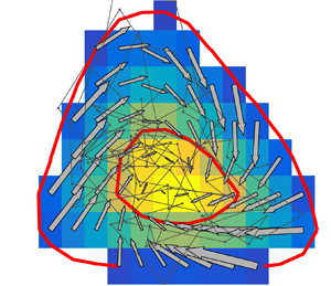
Choosing a variable pair that retains as much deterministic dynamics as possible involves testing 946 possible combinations of two variables. Two examples of the raw material for these tests are shown in figure 1. In each case, the coloured background is the long-time joint probability distribution of the two variables, compiled over a regular partition of either  $m_1\times m_2=15\times 13$ or $21\times 20$ cells along the first and second variable. Results are relatively insensitive to this choice. The finer partition increases the resolution of the results, but decreases their statistical convergence and, to avoid noisy low-probability cells, we always restrict ourselves to the interior of the probability contour containing 95 % of the data. Each cell along the edge of this region approximately contains 300 data points for the coarser partition and 150 for the finer one. The temporal probability flux is represented by vectors joining the centre of each cell with the average location of the points in the cell after one time step, and how much dynamics is left in the projected plane can be estimated from how organised these vectors are (Jiménez Reference Jiménez2023). Most cases are as in figure 1(a), where the state migrates towards the high-probability core of the distribution, essentially driven by entropy. We will denote this variable combination as Case I. A few variable pairs are more organised, as Case II in figure 1(b), whose upper edge is the burst described above. The inclination angle in the abscissae evolves from a backward to a forward tilt, while the intensity in the ordinates first grows and then decays.
Probability distribution and flux vectors for two pairs of projection variables. The arrows link the centre of each partition cell with the mean location of the flow after a time iteration. The red contours enclose 0.3 and 0.95 of the probability mass. (a) A typical disorganised variable pair (Case I). (b) The well-organised Orr burst described in the text (Case II). Here  $\Delta t^*=0.075$; $21\times 20$ cells; C950 (adapted from Jiménez Reference Jiménez2023).

The probability maps in figure 1 include a deterministic component, and a disorganised one that represents the effect of the discarded variables. The latter typically increases with the time increment and dominates for  $\Delta t^*\ge 0.2$, but we will see below that short time increments have problems linked with resolution, and that the limit $\Delta t\to 0$ implies infinitesimally small partition cells. The latter are limited by the amount of training data, and our models are necessarily discrete both in state space and in time.
3. Results
We now describe Markovian models that approximate the order in which the flow visits the partition cells by iterating (2.1). None of them can fully represent the coarse-grained dynamical system, which is generally not Markovian (Beck & Schlögl Reference Beck and Schlögl1993), but we will be interested in how far the approximation can be expected to hold, as explained at the end of the introduction.
The simplest model based on the transition operator is to substitute time stepping by the transition from each partition cell at time  $t$ to the cell containing the average position of its descendants at $t+\Delta t$. Figure 2(a) shows that this is not effective. Although the model follows at first the trend of the probability flow, it drifts towards the dense core of the probability distribution. Some of the core cells are absorbers, i.e. they can be entered but not exited, and the model eventually settles into one of them. Substituting the average position by another deterministic rule, such as the most probable location, leads to similar results.
(a) A deterministic reduced-order model for the Case II variables. Several initial conditions are marked by solid symbols, and the model transitions from a cell at  $t$ to the mean expected position of the system at $t+\Delta t$. After some iterations, all trajectories settle to the cells marked by open symbols. Here $\Delta t^*=0.075$; C950; $15\times 13$ cells. (b) Cell classification for the model in (a). White cells are not visited during training. Yellow cells are absorbers. Blue are regular cells. (c) Fraction of absorbing cells for different deterministic models: $\circ$, $21\times 20$ cells; $\triangle$, $15\times 13$. Black, C950; red, C550.

General theory requires that, if a model is to approximate the statistics of its training run, it should not contain absorbing cells (Feller Reference Feller1971). This depends on the ratio between the time step and the coarseness of the partition. Intuitively, if the ‘state-space velocity’ of a model is  $V_X$ and the ‘cell dimension’ is $\Delta X$, any process with $\Delta t< \Delta X/V_X$ never leaves its cell.
If we assume that the model explores the  $m_p$ cells along the diameter of a partition with a characteristic time $T_{s}$, the relevant normalisation of the ratio between temporal and spatial resolution is $m_p\Delta t /T_{s}$. Figure 2(b) shows the cell classification for the model in figure 2(a). The four yellow cells contain the mean position of their next iteration, and are absorbers. Figure 2(c) shows the fraction of cells that are absorbers, $N_{fix}$, with respect to the $N_{tot}$ active cells (i.e. those visited during training) for different Reynolds numbers and partition resolutions. A dimensionless time based on the resolution along the two coordinate axes, $\Delta t^{{\dagger}} = \Delta t^* \sqrt {m_1 m_2}$, collapses the data reasonably well and the figure shows that the model in figure 2(a) contains at least one absorbing cell even when $\Delta t\gg \tau$, in which limit there is essentially no dynamics left in the operator. The distance between markers along the trajectories in figure 2(a) $(\Delta t^{{\dagger}} \approx 1.5)$ gives an idea of how far the system moves in one modelling step.
Ergodicity can be restored by including the full probability distribution of the iterates in the transition operator (2.1) instead of deterministic values. The path in figure 3(a) is a random walk over the cell indices, created by choosing at  $t+\Delta t$ a random cell from the probability distribution in the column of $\boldsymbol{\mathsf{Q}}_{\Delta t}$ that contains the descendants of the cell at $t$. In addition, and mostly for cosmetic purposes, the cell selected as $\boldsymbol {q}(t+\Delta t)$ is mapped to a random state within it, $\boldsymbol {X}(t+\Delta t)$. As the path explores state space, it creates a one-step probability map that mimics $\boldsymbol{\mathsf{Q}}_{\Delta t}$, and counteracts the entropic drive towards the core of the distribution by adding temperature. The Perron–Frobenius theorem (Lancaster Reference Lancaster1969; Feller Reference Feller1971) guarantees that the one-step transition operator determines the invariant probability density (IPD) of the Markov chain. Under mild conditions that essentially require that the attractor cannot be separated into unconnected subsets, stochastic matrices have a unique dominant right eigenvector that can be scaled to a probability distribution, with unit eigenvalue. Any initial set of cells from a non-zero column converges to this distribution at long times. Each iteration scheme creates its own PFO and IPD. The invariant density of the deterministic model in figure 2(a) is the set of absorbing cells, which attract all the initial conditions. The long-term distribution of the ‘pretrained’ (PPF) chain in figure 3(a) is indistinguishable from the data used to train it.
(a) As in figure 2(a), for  $n_T=100$ time steps evolved using for each iteration a randomly selected cell from the PFO probability cloud. (b) Typical probability distribution of the one-step iterations of the cell marked by a solid circle: ——, full PFO model; - - - -, using a Gaussian approximation to the true PFO; $\cdot \cdot \cdot \cdot \cdot\, \cdot$, Gaussian approximation with fitted parameters. Here $n_T=10^5$. Contours contain 0.3, 0.95 of the probability mass. (c) Invariant probability densities for the three models in (b). Contours contain 0.3, 0.95 and 0.995 of the probability mass. In the three panels, $\Delta t^*=0.075$; $15\times 13$ cells; C950.

Even if the PPF model is a good representation of the flow statistics, the full transition operator is a large matrix that has to be compiled anew for each set of flow parameters. Moreover, figure 3(b) shows that, although the full operator is a complex structure, at least some of the conditional transition probabilities can be approximated by simpler distributions. The black contour in this figure is the true distribution of the one-step iterations from the cell marked by a solid symbol. The dashed contours are a Gaussian approximation to that probability, with the same first- and second-order moments. The parameters of the Gaussian are smooth functions of the projection variables, at least within the 95 % core of the IPD, and the dotted contours are also Gaussian, but using parameters that have been fitted over the whole IPD with a second-order least-square fit. The three approximations are very similar, and figure 3(c) shows that their IPDs also agree to fairly low probability levels. We will mostly present results for the PPF from now on, although keeping in mind that the simpler approximations may be useful in some cases.
3.1. Fake physics
Figure 3(c) should not be interpreted to mean that the Markovian trajectories are the same as in turbulence. All models quickly diverge from their training trajectory, and, even if this is also true for turbulence trajectories starting from the same cell, the model and turbulence trajectories do not shadow each other. However, the agreement of the probability densities in figure 3(c) suggest that some statistical properties of turbulence may be well predicted by the models. This is true for most of the mean velocity and fluctuation profiles, in which it is hard to distinguish the models from the data. In some cases, such as the mean velocity and the intensity of the fluctuations of the wall-parallel velocity components, this is because the flow statistics are relatively insensitive to the position in the projected subspace. An example is the distribution of the wall shear in figure 4(a). In others, such as the wall-normal velocity fluctuation intensities in figure 4(b), the agreement depends on the convergence of the probability density. Note the different range of the colour bars in figures 4(a) and 4(b). Figure 4(c) shows that even in the case of  $v'$, the fluctuation profile is well represented by the stochastic models. The light grey lines in this figure are intensity profiles for states that project onto individual cells of the IPD. The darker lines, which are compiled for the training data and for the three stochastic Markov models, are long-time averages. They are indistinguishable from each other, even if the profiles belonging to individual cells are quite scattered, and the mean values only agree because the Markov chain converges to the correct probability distribution.
(a) Distribution of the velocity gradient at the wall,  $\partial _y U$, conditioned to individual cells. (b) As in (a), for the maximum of $v'$ of the retained Fourier modes. (c) The thicker lines are fluctuation profiles of the wall-normal velocity for the Markovian models in figure 3, and for the training data. Light grey lines are mean profiles compiled over individual cells of the two-dimensional invariant distribution. Here $n_T=10^5$; $\Delta t^*=0.075$; $21\times 20$ cells; Case II of C950.

More interesting are the temporal aspects of the flow. Most complex dynamical systems have a range of temporal scales, from slow ones that describe long-term dynamics, to fast local-in-time events. In the case of wall-bounded turbulence, a representative slow scale is the bursting period,  $O(h/u_\tau )$ (Flores & Jiménez Reference Flores and Jiménez2010). The PFO, which encodes the transition between closely spaced snapshots, describes the fast time.
Figure 5(a) displays the temporal autocorrelation function,  $\langle \boldsymbol {X}(t) \boldsymbol {X}(t+T)\rangle _t/X'^2$, of one of the model variables, computed independently for the turbulence data and for the Markov chain of the PPF model. They approximately agree up to $T^*\approx 0.3$. The correlation of a particular variable depends on how it is distributed over the IPD, but is bounded by the decorrelation of the probability distribution itself, which approaches the IPD with the number, n, of iterations as $|\lambda _{\Delta t}|^n$, where $\lambda _{\Delta t}$ is the eigenvalue of $\boldsymbol{\mathsf{Q}}_{\Delta t}$ with the second highest modulus (Brémaud Reference Brémaud1999). It is intuitively clear that, if the distribution of $\boldsymbol {q}$ approaches the IPD after a given time interval, independently of the initial conditions, its correlation with those initial conditions also vanishes. Figure 5(a) shows that the Markovian models approximately describe turbulence over times of the order of the probability decorrelation time, which is given by the dashed lines. This decay of the correlation corresponds to the exponential divergence of nearby initial conditions. Figure 5(b) shows how the variable in figure 5(a) diverges among trajectories initially within the same partition cell, averaged over the IPD, and shows that the divergence is complete by the time the correlation has decayed. The PPF model and its Gaussian approximations reproduce this behaviour reasonably well.
Temporal behaviour of turbulence and of the Markovian model. In (a–d), Case II. (a) Temporal autocorrelation function of  $I_{v01}$. The grey solid line is obtained from turbulence. Other solid lines are from the PPF model, and the dashed ones are from the subdominant eigenvalue of the PFO. From blue to red: $\Delta t^*=0.025$, 0.075, 0.125. (b) Root-mean-squared divergence among trajectories starting from the same partition cell, normalised with the standard deviation of the variable in question. The solid black line is from the training data; those with symbols are the PPF model, with colours as in (a). (c) Probability distribution of the time of first return to individual cells, averaged within the 95 % probability contour. The continuous blue line is computed from the PPF; the red one is from the training data, and the dashed one is from a series of cells randomly chosen from the data IPD. For the PPF and random models, $\Delta t^*=0.025$ and $n_T=5\times 10^5$. (d) Mean return time of the training data for individual cells in (c). (e) As in (a), for the disorganised Case I. (f) As in (c) for Case I. In all figures, the partition is $15\times 13$ cells, and C950.

More surprising is that this agreement extends to times of the order of the bursting period,  $T^*=O(1)$. The property of time series that more closely corresponds to periodicity is the first-recurrence time, $T_1$, after which the system returns to a particular cell. Its probability distribution is also a property of the PFO (Feller Reference Feller1971), but can be measured from the time series. Figure 5(c) shows the averaged distribution computed by accumulating for each partition cell the probability of recurring after $T_1$. The red line is turbulence data and the blue one is from the PPF model. They agree for very short times, as expected from figure 5(a,b), and for times longer than a few eddy turnovers. The dashed black line is a time series in which the order of the cells is randomly selected from the IPD. The exponential tails of the three distributions suggest that the long-time behaviour of turbulence and of the PPF is essentially random and memoryless. The discrepancy between the red and blue lines at $T_1^*\approx 0.5$ is the same as in the correlations in figure 5(a), and is characteristic of deterministic projections. More significant is the probability deficit between both solid lines and the randomised dashed line for $T_1^*\lesssim 2$, which is a feature of most variable combinations. That both turbulence and the PPF preserve this difference shows that the PPF encodes enough information to approximately reproduce the bursting period, and that bursting, which is responsible for the longer return periods, is a feature of both turbulence and its PPF approximation. Figure 5(d) shows the mean return time for individual cells and reveals that long-term bursting is a property of the periphery of the IPD.
Figure 5(e,f) repeats the analysis in figures 5(a) and 5(c) for the disorganised Case I. The conclusions from the organised variables also apply to the disorganised ones, but there are some differences. The dashed lines in figure 5(a) are the exponential decay due to the subdominant eigenvalue of the PFO. That they depend on the time interval used in the PFO shows that  $\lambda _{\Delta t}^n \ne \lambda _{n\Delta t}$, and the difference between the two quantities measures the ‘memory’ of the system, which is missing for the Markovian model. On the other hand, the dashed lines for the three $\Delta t$ in figure 5(e) essentially collapse, and they also collapse with the decay of the correlation of the model variable, or with the turbulence data. This suggests that none of these processes keeps memory of previous time steps. In fact, while the return plot in figure 5(f) shows the same probability deficit compared to a random process for short return times as the well-organised case in figure 5(c), the effect is weaker, and so is the excess probability in the long tail. This suggests that the time series in Case I are effectively random, in agreement with figure 1(a).
Hallucinations in large foundation models refer to the generation of plausible but factually incorrect answers (Rawte, Sheth & Das Reference Rawte, Sheth and Das2023). In the context of our experiments, in which data are described rather than predicted, they happen when the model drifts into a cell not visited during training. These unseen but accessible cells are part of the absorbing set of the Markovian model and, to avoid being permanently absorbed by one of them after a first ‘admission of ignorance’, the model is directed to continue from a cell randomly selected from the data IPD. The two middle lines in figure 6(a) show the fraction of restarts required for the two Gaussian approximations of the PPF. It grows as the stochastic component of the PFO increases with the time increment, and is always higher for the globally fitted approximation than for the locally fitted one.
(a) Fraction of required restarts for the three models in figure 3, averaged over 500 experiments:  $\square$, PPF; $\circ$, Gaussian approximation to the true PFO, $\gamma =1$; $\triangledown$, $\gamma =2$; $\triangle$, Gaussian approximation with fitted parameters. Bars are one standard deviation. Here $n_T=10^5$ per experiment; $15\times 13$ cells; Case II of C950. (b) Comparison of the IPDs of Case II for the three Reynolds numbers in table 1. The vertical coordinate is scaled by a factor $\alpha$. ——, C950 and $\alpha =1$; — $\cdot$ —, C550 and $\alpha =0.86$; - - - -, C350 and $\alpha =0.81$. The first and last stretching factors are manually adjusted for optimum fit. The middle one is linearly interpolated from the other two.

The lower black line requires some explanation. The results discussed above are fairly resilient to changes in the training process. All of them were tested with a training set containing half as many data as the present one, and with different combinations of  $y$-filtering and Reynolds number. In no case did the straightforward PPF produce hallucinations in the sense above. This is because the conditional probability distributions are compiled from a continuous data path in which every cell entered is also exited. This is an artificial feature amounting to overfitting. To prevent it, the PFOs used in this paper are compiled by first breaking the training set into segments of $N_{chop}=20$ snapshots. The last snapshot of each segment is entered but not exited during training, and the resulting probabilities are a fairer estimation of the likelihood of hallucinations. It is approximately constant for $N_{chop}\in 5\unicode{x2013}20$, and the lowest line in figure 6(a) is the average miss ratio in this range. None of the lower three lines in the figure is large enough to influence the overall statistics, but it is easy to create models in which hallucinations matter. The simplest one is to modify the local Gaussian approximation by multiplying its second-order moments by a factor $\gamma^2$. The optimum approximation is at $\gamma \approx 1$, as expected, but the restarts become more frequent as larger values of $\gamma$ allow the model to wander into unseen regions. The uppermost line in figure 6(a) is a modified Gaussian model with $\gamma =2$, and the restart fraction reaches almost 10 %.
4. Conclusions
We have shown that, at least for quasideterministic variable pairs, the one-step PFO acts as a surrogate for the differential equations of motion and that, in the same way as the latter generate all the temporal scales of turbulence, the Markov chain induced by the PFO retains substantial physics over all those scales. We have traced the agreement at very short and very long times to general properties of Markov chains, but the agreement for periods of the order of an eddy turnover shows that some non-trivial physics is also retained.
Neither the PFO nor its Markov chains can provide information that was not in the original dynamical system, but they do it more simply. The full PFO is an  $N_D^2$ matrix, where $N_D\sim O(200)$ is the number of cells in the partition. This is already a large reduction from the original number of degrees of freedom, $O(10^6)$, but the Gaussian approximation is a much shorter list of $5N_D$ numbers, and the quadratic fit to the Gaussian parameters only requires 25 numbers, 5 for each Gaussian moment. This economy, besides simplifying calculations, becomes important when interpolating models among cases, such as different Reynolds numbers. Although we have mostly described results for the highest Reynolds number, C950, most also apply to the two lower Reynolds numbers in table 1. An example is figure 6(b), which compares the invariant densities of the three Reynolds numbers, and shows that they mostly differ by a rescaling of the intensity axis. This figure also serves as a test for model interpolation. The highest and lowest Reynolds numbers in the figure are fitted by hand, but the intermediate one is linearly interpolated from them as a function of $Re_\tau$. We have finally shown that the PFO can be substantially modified without much degradation, probably because it is already an approximation.
In essence, the PFO can be understood as a statistical counterpart to the equations of motion, in the sense that both encode the response of the system at every point in a low-dimensional projection of state space. In the case of the PFO, this is obtained from observation and given in terms of probabilities, while in the case of the equations it would be a functional relation if all the variables were known. There are two important differences. The first is that the PFO works on a submanifold, and cannot make exact predictions. The second, and perhaps most significant, is that a PFO derived from passive observations only has information about the system attractor, while the equations of motion, which have presumably been supplemented by experiments outside the attractor, work throughout state space. As a consequence, the former permits a much narrower set of control strategies than what can be analysed by the latter.
Perhaps the most intriguing aspect of the discussion above is how little, beyond the initial choice of a restricted set of variables, is specific to turbulence. Much of the agreement or disagreement between the models and the original system can be traced to generic properties of the transition operator, and should therefore apply to other high-dimensional dynamical systems, or to Markovian ROMs in general, but it is important to emphasise the extreme reduction of dimensionality in the ROMs described here.
Acknowledgements
The author would like to acknowledge informal discussions with many colleagues over months of perplexity, as well as with three patient referees.
Funding
This work was supported by the European Research Council under the Caust grant ERC-AdG-101018287.
Declaration of interests
The author reports no conflict of interest.
Data availability statement
The summary variables used for the paper (a few Gbytes in binary format) are freely available at the group web site, https://torroja.dmt.upm.es/turbdata, together with a basic reading and postprocessing code.


 Open access

