

1 Introduction
The Arthur Trace Formula (ATF) is a vast generalization of the Selberg Trace Formula to arbitrary rank reductive groups. The first incarnation of ATF, the noninvariant trace formula, relies on two crucial ingredients: the integral of a truncated kernel (of a compactly supported test function) is absolutely convergent, and the integral depends polynomially on the truncation parameter (which he has to assume is sufficiently regular). The purpose of this work is to prove two general, purely combinatorial, statements about polytopes, one on convergence and the other on polynomiality of certain integrals. These statements essentially capture, and generalize, the combinatorial aspects of Arthur’s corresponding results (cf. [Reference ArthurAr78, Reference ArthurAr81]), isolating them from the analytic aspects that use reduction theory and other techniques. The long-term hope for our project, of which this work is a first step, is to aim at applications of the ATF to more general test functions [Reference Finis and LapidFL11, Reference Finis and LapidFL16, Reference Finis, Lapid and MüllerFLM11, Reference HoffmannHoff08].
We also give interpretations of our combinatorial results in terms of the geometry of toric varieties. We hope the present paper would shed light on the combinatorics behind ATF and its similarity with certain concepts appearing in toric geometry. The connection between polyhedral combinatorics appearing in Arthur’s trace formula and in toric varieties is not quite transparent yet. In this regard, we mention the articles of Kottwitz [Reference KottwitzKot05] and Finis and Lapid [Reference Finis and LapidFL11], which may be relevant.
We now briefly recall the trace formula before explaining a summary of our results and proofs.
1.1 Arthur’s noninvariant trace formula
For a finite group G, the character of a representation of G (or any conjugation invariant function on G for that matter) can be written uniquely as a linear combination of characteristic functions of different conjugacy classes, as well as, a linear combination of traces of irreducible representations. The equality of these two decompositions is a special case of the Frobenius Reciprocity, which plays an important role in representation theory of finite groups. This is the prototype of many trace formulas in representation theory.
Arthur gave a far reaching trace formula for arbitrary reductive groups defined over number fields. A main problem is that in this generality, the integral representing the trace diverges. Arthur introduces an operation of truncation to modify this integral so that it becomes convergent.
The (noninvariant) ATF is an equality of two distributions:
 $$ \begin{align} J_{\textrm{geom}}(f) = J_{\textrm{spec}}(f), \quad f \in C_c^{\infty}(G({\mathbb A})^1). \end{align} $$
Here, G is a connected reductive linear algebraic group defined over ${\mathbb Q}$
(or any number field) whose ring of adeles we denote by
${\mathbb Q}$
(or any number field) whose ring of adeles we denote by ${\mathbb A}$
and
${\mathbb A}$
and $G({\mathbb A})^1$
consists of those
$G({\mathbb A})^1$
consists of those $x \in G({\mathbb A})$
satisfying
$x \in G({\mathbb A})$
satisfying $|\chi (x)|_{\mathbb A} = 1$
for all rational characters
$|\chi (x)|_{\mathbb A} = 1$
for all rational characters $\chi $
of G. Both the geometric and the spectral distributions on the two sides of (1.1) are equal to the integral over
$\chi $
of G. Both the geometric and the spectral distributions on the two sides of (1.1) are equal to the integral over $G({\mathbb Q}) \backslash G({\mathbb A})^1$
of a modified kernel
$G({\mathbb Q}) \backslash G({\mathbb A})^1$
of a modified kernel $k^T(x) = k^T(x,f)$
at a certain value
$k^T(x) = k^T(x,f)$
at a certain value $T=T_0$
of a suitably regular truncation parameter T belonging to the positive Weyl chamber of G with respect to a fixed minimal parabolic subgroup. The space
$T=T_0$
of a suitably regular truncation parameter T belonging to the positive Weyl chamber of G with respect to a fixed minimal parabolic subgroup. The space $G({\mathbb Q}) \backslash G({\mathbb A})^1$
is in general finite volume (with respect to the Haar measure on G), but only compact when G has no proper parabolic subgroups. While the trace formula in the case of compact quotient was well understood, already the development of the trace formula in the case of
$G({\mathbb Q}) \backslash G({\mathbb A})^1$
is in general finite volume (with respect to the Haar measure on G), but only compact when G has no proper parabolic subgroups. While the trace formula in the case of compact quotient was well understood, already the development of the trace formula in the case of $\textrm {SL}(2,{\mathbb Z}) \backslash \textrm {SL}(2,{\mathbb R})$
led Selberg to his celebrated Selberg Trace Formula. However, Arthur realized that the presence of proper parabolic subgroups in a more general group G makes the integral of the kernel function divergent. As a result, he introduced the modified kernel
$\textrm {SL}(2,{\mathbb Z}) \backslash \textrm {SL}(2,{\mathbb R})$
led Selberg to his celebrated Selberg Trace Formula. However, Arthur realized that the presence of proper parabolic subgroups in a more general group G makes the integral of the kernel function divergent. As a result, he introduced the modified kernel $k^T(x)$
. Two major properties of the modified kernel (see [Reference ArthurAr78, Reference ArthurAr81]) are the following:
$k^T(x)$
. Two major properties of the modified kernel (see [Reference ArthurAr78, Reference ArthurAr81]) are the following:
-
(1) $\int \limits _{G({\mathbb Q}) \backslash G({\mathbb A})^1} |k^T(x)| \, dx < \infty $
for suitably regular truncation parameter T.
$\int \limits _{G({\mathbb Q}) \backslash G({\mathbb A})^1} |k^T(x)| \, dx < \infty $
for suitably regular truncation parameter T. -
(2) The function
$ T \mapsto J^T(f) = \int \limits _{G({\mathbb Q}) \backslash G({\mathbb A})^1} k^T(x) \, dx $
is a polynomial function of T.


As the truncation parameter T goes further away from the origin, the integral of $k^T(x)$
gets closer to the (divergent) integral representing the trace. Among other things, the proofs involve quite intricate combinatorics of convex polytopes and convex cones. Expanding the modified kernel geometrically (via conjugacy classes) and spectrally (via automorphic representations) then provides the two sides of (the truncated analogue of) the identity (1.1).
$k^T(x)$
gets closer to the (divergent) integral representing the trace. Among other things, the proofs involve quite intricate combinatorics of convex polytopes and convex cones. Expanding the modified kernel geometrically (via conjugacy classes) and spectrally (via automorphic representations) then provides the two sides of (the truncated analogue of) the identity (1.1).
In the function field case, one also has an analogue of the ATF and the truncation parameter T. In particular, we mention the work of Laumon [Reference LaumonLau96, Reference LaumonLau97] where he develops the trace formula for certain class of test functions for which the modified kernel $k^T(\cdot )$
turns out to be equal to the usual kernel
$k^T(\cdot )$
turns out to be equal to the usual kernel $k(\cdot )$
. This makes the question of polynomiality obvious since the resulting polynomials would simply be constant. However, the convergence question still remains and indeed a similar argument as Arthur’s in the number field case applies.
$k(\cdot )$
. This makes the question of polynomiality obvious since the resulting polynomials would simply be constant. However, the convergence question still remains and indeed a similar argument as Arthur’s in the number field case applies.
1.2 Main results
We introduce a notion of combinatorial truncation and prove two main results on its convergence and polynomiality. The idea for our results is to start with a complex-valued function on a finite dimensional real vector space whose integral over the vector space is possibly divergent. We then “truncate” this function by subtracting some other functions around some neighborhoods of infinity to arrive at a “truncated function” whose integral over the vector space is absolutely convergent. The “neighborhoods of infinity” are with respect to a toric compactification of V (in the sense of Sections 5.1 and 5.3) whose data are encoded in a polytope and its normal fan. We then prove that the integral of the truncated function, as a function of the polytope, is indeed a polynomial function.
To explain our results, we introduce some notation and refer to Sections 2.1 and 2.2 for further details on convex cones and polytopes. We first explain our convergence results.
Let $V \cong {\mathbb R}^n$
be an n-dimensional real vector space. We fix an inner product
$V \cong {\mathbb R}^n$
be an n-dimensional real vector space. We fix an inner product $\langle \cdot , \cdot \rangle $
on V and use it to identify V with its dual
$\langle \cdot , \cdot \rangle $
on V and use it to identify V with its dual $V^*$
. Fix a full dimensional, complete, simplicial fan
$V^*$
. Fix a full dimensional, complete, simplicial fan $\Sigma $
in V and fix a polytope
$\Sigma $
in V and fix a polytope $\Delta \in {\mathcal P}(\Sigma )$
, the set of polytopes with normal fan
$\Delta \in {\mathcal P}(\Sigma )$
, the set of polytopes with normal fan $\Sigma $
(see Figure 1). There is a one-to-one correspondence between the cones in
$\Sigma $
(see Figure 1). There is a one-to-one correspondence between the cones in $\Sigma $
and the faces of
$\Sigma $
and the faces of $\Delta $
. For
$\Delta $
. For $\sigma \in \Sigma $
, we let
$\sigma \in \Sigma $
, we let $T^-_{\Delta , \sigma }$
denote the outward-looking tangent cone of
$T^-_{\Delta , \sigma }$
denote the outward-looking tangent cone of $\Delta $
at the face corresponding to
$\Delta $
at the face corresponding to $\sigma $
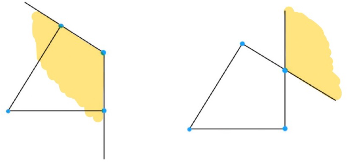
(see Section 2.2 and Figures 3 and 4).
$\sigma $
(see Section 2.2 and Figures 3 and 4).
(Left) A complete simplicial fan in $V={\mathbb R}^2$
; we have labeled three cones in the fan. (Right) A polygon normal to the fan and regions obtained by drawing the outward face cones; the function
$V={\mathbb R}^2$
; we have labeled three cones in the fan. (Right) A polygon normal to the fan and regions obtained by drawing the outward face cones; the function $k_\Delta $
in the shaded region is given by
$k_\Delta $
in the shaded region is given by $K_{0} -K_{1}-K_{2}+K_{12}$
.
$K_{0} -K_{1}-K_{2}+K_{12}$
.
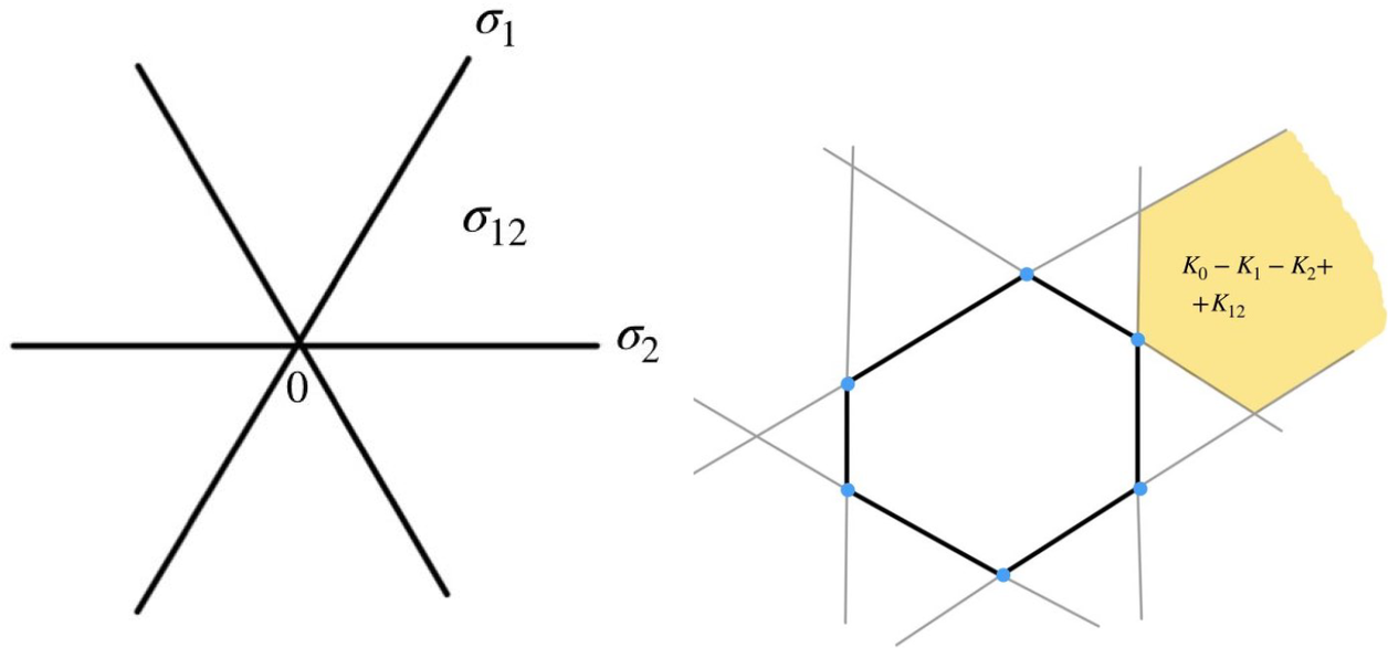
Illustration of the truncated function $k_\Delta $
for when
$k_\Delta $
for when $\Delta $
is a line segment.
$\Delta $
is a line segment.
Inward and outward tangent cones at a vertex (left inward, right outward).
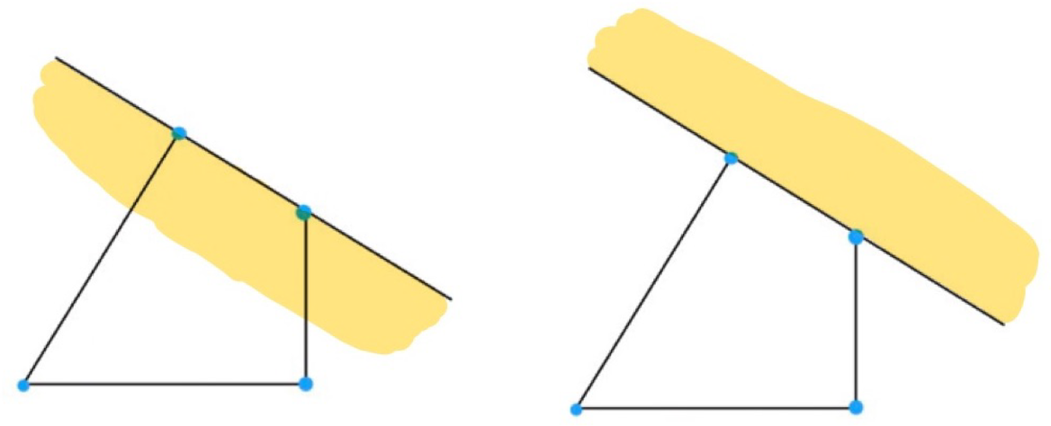
Inward and outward tangent cones at an edge (left inward, right outward).
Suppose a function $K_0: V \to {{\mathbb C}}$
is given with
$K_0: V \to {{\mathbb C}}$
is given with $\int_V K_0(x) \, dx$
possibly divergent. In fact, let
$\int_V K_0(x) \, dx$
possibly divergent. In fact, let $K_0$
be a member of a collection of functions
$K_0$
be a member of a collection of functions $K_\sigma : V \to {\mathbb C}$
, one for each
$K_\sigma : V \to {\mathbb C}$
, one for each $\sigma \in \Sigma $
. We will assume that
$\sigma \in \Sigma $
. We will assume that $K_\sigma $
is invariant in the direction of
$K_\sigma $
is invariant in the direction of $\operatorname {Span}(\sigma )$
, i.e.,
$\operatorname {Span}(\sigma )$
, i.e., $K_\sigma (x+y) = K_\sigma (x)$
for
$K_\sigma (x+y) = K_\sigma (x)$
for $x \in V$
and
$x \in V$
and $y \in \operatorname {Span}(\sigma )$
.
$y \in \operatorname {Span}(\sigma )$
.
Associated with the collection $(K_\sigma )_{\sigma \in \Sigma }$
and the polytope
$(K_\sigma )_{\sigma \in \Sigma }$
and the polytope $\Delta $
, we define the truncated function
$\Delta $
, we define the truncated function
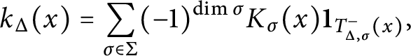 $$ \begin{align} k_\Delta(x) = \sum\limits_{\sigma \in \Sigma} (-1)^{\dim \sigma} K_{\sigma}(x) {\textbf 1}_{T^-_{\Delta, \sigma}(x)}, \end{align} $$
where ${\textbf 1}$
denotes the characteristic function. We think of
${\textbf 1}$
denotes the characteristic function. We think of $k_\Delta (x)$
as a “truncation” of
$k_\Delta (x)$
as a “truncation” of $K_0$
by means of the polytope
$K_0$
by means of the polytope $\Delta $
and the functions
$\Delta $
and the functions $K_\sigma $
for nonzero cones
$K_\sigma $
for nonzero cones $\sigma \in \Sigma $
.
$\sigma \in \Sigma $
.
Note that the function $k_{\Delta }(x)$
and
$k_{\Delta }(x)$
and $K_0(x)$
coincide for
$K_0(x)$
coincide for $x \in \Delta $
. In fact, if all the
$x \in \Delta $
. In fact, if all the $K_\sigma $
are identically equal to
$K_\sigma $
are identically equal to $1$
, by the classical Brianchon–Gram theorem (cf. Theorem 2.6), the function
$1$
, by the classical Brianchon–Gram theorem (cf. Theorem 2.6), the function $k_\Delta (x)$
coincides with the characteristic function of
$k_\Delta (x)$
coincides with the characteristic function of $\Delta $
(see Section 1.4).
$\Delta $
(see Section 1.4).
One of our main results gives a sufficient condition for $k_\Delta (x)$
to be absolutely integrable on V (see Theorem 3.4 and also Theorem 3.5).
$k_\Delta (x)$
to be absolutely integrable on V (see Theorem 3.4 and also Theorem 3.5).
For $\sigma _2 \preceq \sigma _1$
in
$\sigma _2 \preceq \sigma _1$
in $\Sigma $
, let
$\Sigma $
, let
 $$\begin{align*}K_{\sigma_1, \sigma_2}(x) = \sum_{\sigma_2 \preceq \tau \preceq \sigma_1} (-1)^{\dim \tau} K_{\tau}(x). \end{align*}$$
Also, let polyhedral regions $R_{\sigma _1}^{\sigma _2}$
and
$R_{\sigma _1}^{\sigma _2}$
and $S_{\sigma _1}^{\sigma _2}$
be as in Definition 3.2, i.e.,
$S_{\sigma _1}^{\sigma _2}$
be as in Definition 3.2, i.e., $S_{\sigma _1}^{\sigma _2}$
is the cone in
$S_{\sigma _1}^{\sigma _2}$
is the cone in $\operatorname {Span}(\sigma _1)$
defined via the edge vectors and facet normals of
$\operatorname {Span}(\sigma _1)$
defined via the edge vectors and facet normals of $\sigma _1$
and
$\sigma _1$
and $\sigma _2$
as in Definition 3.2(a) (or equivalently (3.10)) and
$\sigma _2$
as in Definition 3.2(a) (or equivalently (3.10)) and $R_{\sigma _1}^{\sigma _2} = Q_{\sigma _1} + S_{\sigma _1}^{\sigma _2}$
, where
$R_{\sigma _1}^{\sigma _2} = Q_{\sigma _1} + S_{\sigma _1}^{\sigma _2}$
, where $Q_{\sigma _1}$
is the face of
$Q_{\sigma _1}$
is the face of $\Delta $
associated with the cone
$\Delta $
associated with the cone $\sigma \in \Sigma $
.
$\sigma \in \Sigma $
.
Convergence Assume that the fan $\Sigma $
above is acute (cf. Definition 3.1
). With the notation as above, suppose for any
$\Sigma $
above is acute (cf. Definition 3.1
). With the notation as above, suppose for any $\sigma _2 \preceq \sigma _1$
, the function
$\sigma _2 \preceq \sigma _1$
, the function $K_{\sigma _1, \sigma _2}$
is rapidly decreasing on the shifted neighborhoods of
$K_{\sigma _1, \sigma _2}$
is rapidly decreasing on the shifted neighborhoods of $S^{\sigma _1}_{\sigma _2}$
. (See Theorem 3.5 for the precise definition.) Then for any polytope
$S^{\sigma _1}_{\sigma _2}$
. (See Theorem 3.5 for the precise definition.) Then for any polytope $\Delta \in {\mathcal P}(\Sigma )$
, the integral
$\Delta \in {\mathcal P}(\Sigma )$
, the integral
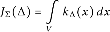 $$\begin{align*}J_{\Sigma}(\Delta) = \int\limits_V k_\Delta(x) \, dx \end{align*}$$
is absolutely convergent.
We note that the conditions on $K_{\sigma _1, \sigma _2}$
in the theorem are “local” with respect to the fan
$K_{\sigma _1, \sigma _2}$
in the theorem are “local” with respect to the fan $\Sigma $
in the sense that for each
$\Sigma $
in the sense that for each $\sigma \in \Sigma $
, we only need to check a condition about
$\sigma \in \Sigma $
, we only need to check a condition about $\sigma $
and the functions
$\sigma $
and the functions $K_\tau $
,
$K_\tau $
, $\tau \preceq \sigma $
(and independent of other cones in the fan and their associated functions).
$\tau \preceq \sigma $
(and independent of other cones in the fan and their associated functions).
We also remark that the assumption that the fan $\Sigma $
is acute is crucial; without it, the convergence result may fail as we show in Example 3.6 where we consider obtuse cones.
$\Sigma $
is acute is crucial; without it, the convergence result may fail as we show in Example 3.6 where we consider obtuse cones.
Next, we discuss our result on polynomiality. The set ${\mathcal P}(\Sigma )$
of polytopes with normal fan
${\mathcal P}(\Sigma )$
of polytopes with normal fan $\Sigma $
is closed under multiplication by positive scalars and the Minkowski sum. Hence, it makes sense to talk about a polynomial function on
$\Sigma $
is closed under multiplication by positive scalars and the Minkowski sum. Hence, it makes sense to talk about a polynomial function on ${\mathcal P}(\Sigma )$
. In fact, if
${\mathcal P}(\Sigma )$
. In fact, if $\Sigma (1)$
denotes the set of one-dimensional cones in
$\Sigma (1)$
denotes the set of one-dimensional cones in $\Sigma $
, then a polytope
$\Sigma $
, then a polytope $\Delta \in {\mathcal P}(\Sigma )$
has a unique representation as
$\Delta \in {\mathcal P}(\Sigma )$
has a unique representation as
 $$\begin{align*}\Delta = \{ x \in V : \langle x, v_\rho \rangle \geqslant a_\rho, \forall \rho \in \Sigma(1)\}, \end{align*}$$
where $v_\rho $
denotes the unit vector along
$v_\rho $
denotes the unit vector along $\rho $
. The numbers
$\rho $
. The numbers $(a_\rho )_{\rho \in \Sigma (1)}$
are called the support numbers of
$(a_\rho )_{\rho \in \Sigma (1)}$
are called the support numbers of $\Delta $
and can be considered as coordinates on
$\Delta $
and can be considered as coordinates on ${\mathcal P}(\Sigma )$
(see Section 2.3). Our main polynomiality result (cf. Theorem 4.1) states that the integral of
${\mathcal P}(\Sigma )$
(see Section 2.3). Our main polynomiality result (cf. Theorem 4.1) states that the integral of $k_\Delta (x)$
depends polynomially on
$k_\Delta (x)$
depends polynomially on $\Delta \in {\mathcal P}(\Sigma )$
.
$\Delta \in {\mathcal P}(\Sigma )$
.
Polynomiality The function
 $$ \begin{align*}\Delta \mapsto J_{\Sigma}(\Delta)\end{align*} $$
is a polynomial on ${\mathcal P}(\Sigma )$
, i.e., a polynomial in the support numbers of
${\mathcal P}(\Sigma )$
, i.e., a polynomial in the support numbers of $\Delta $
.
$\Delta $
.
We remark that if all the $K_\sigma $
are identically equal to
$K_\sigma $
are identically equal to $1$
, then
$1$
, then $J_{\Sigma }(\Delta )$
coincides with the volume of
$J_{\Sigma }(\Delta )$
coincides with the volume of $\Delta $
. Thus, our Polynomiality Theorem is a vast generalization of the classical fact that
$\Delta $
. Thus, our Polynomiality Theorem is a vast generalization of the classical fact that $\Delta \mapsto \operatorname {vol}(\Delta )$
is a polynomial function. The assumption that each
$\Delta \mapsto \operatorname {vol}(\Delta )$
is a polynomial function. The assumption that each $K_\sigma $
is invariant in the direction of
$K_\sigma $
is invariant in the direction of $\operatorname {Span}(\sigma )$
is obviously crucial in the proof of the Polynomiality Theorem. For example, one can consider examples where
$\operatorname {Span}(\sigma )$
is obviously crucial in the proof of the Polynomiality Theorem. For example, one can consider examples where $K_\sigma $
are not necessarily constant, but rather they are asymptotic to a constant in the direction of
$K_\sigma $
are not necessarily constant, but rather they are asymptotic to a constant in the direction of $\operatorname {Span}(\sigma )$
. Then one can still have convergence of
$\operatorname {Span}(\sigma )$
. Then one can still have convergence of $J_{\Sigma }(\Delta )$
by our more general Theorem 3.4 on convergence, while
$J_{\Sigma }(\Delta )$
by our more general Theorem 3.4 on convergence, while $J_{\Sigma }(\Delta )$
would clearly not be a polynomial function.
$J_{\Sigma }(\Delta )$
would clearly not be a polynomial function.
The strategy to prove our Convergence Theorem is as follows. Recall that the truncated function $k_\Delta (x)$
in (1.2) is defined as an alternating sum over various outward tangent cones
$k_\Delta (x)$
in (1.2) is defined as an alternating sum over various outward tangent cones $T^-_{\Delta , \sigma }$
. In Lemma 3.3, we prove a certain double partition of the tangent cones
$T^-_{\Delta , \sigma }$
. In Lemma 3.3, we prove a certain double partition of the tangent cones $T^-_{\Delta , \sigma }$
in terms of certain natural subsets that appear, associated with pairs of cones in
$T^-_{\Delta , \sigma }$
in terms of certain natural subsets that appear, associated with pairs of cones in $\Sigma $
, with the smaller cone being a face of
$\Sigma $
, with the smaller cone being a face of $\sigma $
and the large one having
$\sigma $
and the large one having $\sigma $
as a face. In the double partition, the inner partition essentially amounts to the special case where
$\sigma $
as a face. In the double partition, the inner partition essentially amounts to the special case where $\sigma $
is a full dimensional cone in
$\sigma $
is a full dimensional cone in $\Sigma $
, whereas the outer partition amounts to a “nearest face partition” (cf. Section 2.4). This allows us to repackage the various terms appearing in
$\Sigma $
, whereas the outer partition amounts to a “nearest face partition” (cf. Section 2.4). This allows us to repackage the various terms appearing in $k_\Delta $
into a sum of certain alternating sums
$k_\Delta $
into a sum of certain alternating sums $K_{\sigma _1,\sigma _2}$
associated with pairs of cones
$K_{\sigma _1,\sigma _2}$
associated with pairs of cones $\sigma _2 \preceq \sigma _1$
in
$\sigma _2 \preceq \sigma _1$
in $\Sigma $
. As a result, we reduce the question of the absolute convergence of the integral of
$\Sigma $
. As a result, we reduce the question of the absolute convergence of the integral of $k_\Delta (x)$
over V to that of absolute convergence of
$k_\Delta (x)$
over V to that of absolute convergence of $K_{\sigma _1,\sigma _2}$
on the sets we obtain out of the partition. This already gives our first, and more general, convergence result (cf. Theorem 3.4). We then go on to show that the two conditions in the above convergence theorem guarantee the convergence of the integral of
$K_{\sigma _1,\sigma _2}$
on the sets we obtain out of the partition. This already gives our first, and more general, convergence result (cf. Theorem 3.4). We then go on to show that the two conditions in the above convergence theorem guarantee the convergence of the integral of $K_{\sigma _1,\sigma _2}$
on the required sets.
$K_{\sigma _1,\sigma _2}$
on the required sets.
The regions we mentioned above seem to show up naturally in any treatment of convergence results, including Arthur’s original proof of convergence of his (noninvariant) trace formula. When $\sigma _1$
is full dimensional (corresponding to a maximal parabolic subgroup in Arthur’s setting) and
$\sigma _1$
is full dimensional (corresponding to a maximal parabolic subgroup in Arthur’s setting) and $\sigma _2$
is the origin, the region simply becomes the cone
$\sigma _2$
is the origin, the region simply becomes the cone $\sigma _1$
shifted to the vertex of
$\sigma _1$
shifted to the vertex of $\Delta $
corresponding to
$\Delta $
corresponding to $\sigma _1$
. When
$\sigma _1$
. When $\sigma _2$
is a nonzero face of
$\sigma _2$
is a nonzero face of $\sigma _1$
, then the region is again another cone shifted to the vertex. This type of cone is precisely what Arthur has, for example, in [Reference ArthurAr05, Figure 8.5]. For more general
$\sigma _1$
, then the region is again another cone shifted to the vertex. This type of cone is precisely what Arthur has, for example, in [Reference ArthurAr05, Figure 8.5]. For more general $\sigma _1$
, the regions are a sum (as a set) of a compact face of
$\sigma _1$
, the regions are a sum (as a set) of a compact face of $\Delta $
and a somewhat simpler cone. For example, when
$\Delta $
and a somewhat simpler cone. For example, when $\dim V = 2$
, these regions look like stripes.
$\dim V = 2$
, these regions look like stripes.
A key step in the proof of the Polynomiality Theorem is Lemma 4.6, which is a statement concerning the polytope $\Delta $
and a cone
$\Delta $
and a cone $\sigma \in \Sigma $
. As far as we know, this lemma is new and does not appear in Arthur’s work. It simplifies and streamlines some of the combinatorial arguments in [Reference ArthurAr78, Reference ArthurAr81]. As a special case when
$\sigma \in \Sigma $
. As far as we know, this lemma is new and does not appear in Arthur’s work. It simplifies and streamlines some of the combinatorial arguments in [Reference ArthurAr78, Reference ArthurAr81]. As a special case when $\Delta = \{0\}$
, Lemma 4.6 also implies the Langlands combinatorial lemma (see [Reference ArthurAr05, equations (8.10) and (8.11)], [Reference Goresky, Kottwitz and MacPhersonGKM97, Appendix]).
$\Delta = \{0\}$
, Lemma 4.6 also implies the Langlands combinatorial lemma (see [Reference ArthurAr05, equations (8.10) and (8.11)], [Reference Goresky, Kottwitz and MacPhersonGKM97, Appendix]).
When $\sigma $
is full dimensional and the vertex of
$\sigma $
is full dimensional and the vertex of $\Delta $
corresponding to
$\Delta $
corresponding to $\sigma $
lies in
$\sigma $
lies in $\sigma $
, Lemma 4.6 gives a decomposition of the characteristic function of the polytope
$\sigma $
, Lemma 4.6 gives a decomposition of the characteristic function of the polytope $\Delta \cap \sigma $
in terms of certain cones with apexes at the vertices of this polytope. We obtain Lemma 4.6 as a corollary of the Lawrence–Varchenko conical decomposition of a polytope (Theorem 2.8). In fact, we need a more general version of this decomposition that applies to virtual polytopes (Theorem 2.10). The arguments in this section rely on some key concepts and results from [Reference Khovanskii and PukhlikovKP93a, Reference Khovanskii and PukhlikovKP93b] (which we review in Section 2.6). We would like to point out that the proof of polynomiality shows that
$\Delta \cap \sigma $
in terms of certain cones with apexes at the vertices of this polytope. We obtain Lemma 4.6 as a corollary of the Lawrence–Varchenko conical decomposition of a polytope (Theorem 2.8). In fact, we need a more general version of this decomposition that applies to virtual polytopes (Theorem 2.10). The arguments in this section rely on some key concepts and results from [Reference Khovanskii and PukhlikovKP93a, Reference Khovanskii and PukhlikovKP93b] (which we review in Section 2.6). We would like to point out that the proof of polynomiality shows that $J_{\Sigma }(\Delta )$
is a linear combination of volumes of certain virtual polytopes
$J_{\Sigma }(\Delta )$
is a linear combination of volumes of certain virtual polytopes $\Gamma _{\Delta , \sigma }$
,
$\Gamma _{\Delta , \sigma }$
, $\sigma \in \Sigma $
.
$\sigma \in \Sigma $
.
In the interest of making the connections with poset theory and Möbius inversion more transparent, we show that the Langlands combinatorial lemma can be interpreted as a formula for the inverse of a certain element in the incidence algebra of the poset of faces of a polyhedral cone (see Corollary 4.7).
Finally, we point out that Arthur’s truncation parameter T determines a polytope which is the convex hull of the Weyl group orbit of T. Thus, Arthur’s combinatorics is concerned with Weyl group invariant polytopes with a vertex in each Weyl chamber. In this paper, we generalize the combinatorics to arbitrary simple polytopes.
It follows from the proof of polynomiality that
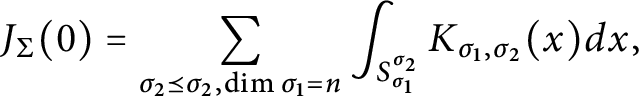 $$\begin{align*}J_{\Sigma}(0) = \sum_{\sigma_2 \preceq \sigma_2, \dim \sigma_1 = n} \int_{S_{\sigma_1}^{\sigma_2}} K_{\sigma_1, \sigma_2}(x) dx, \end{align*}$$
and that, in the case of a Weyl fan $\Sigma $
and a Weyl group invariant
$\Sigma $
and a Weyl group invariant $\Delta $
, the top degree homogeneous part of the polynomial
$\Delta $
, the top degree homogeneous part of the polynomial $J_{\Sigma }(\Delta )$
is a constant multiple of the volume of
$J_{\Sigma }(\Delta )$
is a constant multiple of the volume of $\Delta $
.
$\Delta $
.
1.3 The simplest example
Let $\Sigma $
be the complete fan in
$\Sigma $
be the complete fan in $V = {\mathbb R}$
consisting of the origin
$V = {\mathbb R}$
consisting of the origin $\sigma _0 = \{0\}$
, the negative half-line
$\sigma _0 = \{0\}$
, the negative half-line $\sigma _-$
, and the positive half-line
$\sigma _-$
, and the positive half-line $\sigma _+$
. Let
$\sigma _+$
. Let $\Delta \subset V^* \cong V = {\mathbb R}$
be the line segment
$\Delta \subset V^* \cong V = {\mathbb R}$
be the line segment $[a, b]$
. Let
$[a, b]$
. Let $K_0$
,
$K_0$
, $K_-$
, and
$K_-$
, and $K_+$
be functions on V corresponding to
$K_+$
be functions on V corresponding to $\sigma _0$
,
$\sigma _0$
, $\sigma _-$
, and
$\sigma _-$
, and $\sigma _+$
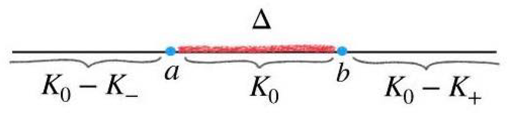
, respectively. From definition, one computes that the truncated function
$\sigma _+$
, respectively. From definition, one computes that the truncated function $k_\Delta (x)$
is given by (see Figure 2).
$k_\Delta (x)$
is given by (see Figure 2).
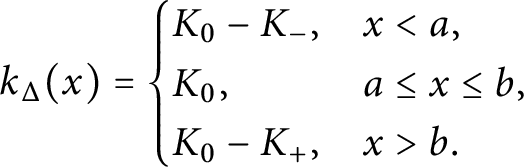 $$\begin{align*}k_\Delta(x) = \begin{cases} K_0 - K_-, & x < a, \\ K_0, & a \leq x \leq b, \\ K_0 - K_+, & x> b. \\ \end{cases} \end{align*}$$
The assumption in Theorem 4.1 that $K_\sigma $
is constant along
$K_\sigma $
is constant along $\operatorname {Span}(\sigma )$
implies that
$\operatorname {Span}(\sigma )$
implies that $K_-$
and
$K_-$
and $K_+$
are constant functions. Moreover, the condition that
$K_+$
are constant functions. Moreover, the condition that $\int \limits _{V} k_\Delta (x) dx$
is absolutely convergent means that
$\int \limits _{V} k_\Delta (x) dx$
is absolutely convergent means that $|K_0(x) - K_-|$
and
$|K_0(x) - K_-|$
and $|K_0(x) - K_+|$
are integrable. We have
$|K_0(x) - K_+|$
are integrable. We have
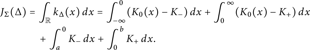 $$\begin{align*}J_{\Sigma}(\Delta) &= \int_{\mathbb R} k_\Delta(x) \, dx = \int_{-\infty}^0 (K_0(x) - K_-) \, dx + \int_0^{\infty} (K_0(x) - K_+) \, dx\\[-1pt] &\quad + \int_a^0 K_- \, dx + \int_0^b K_+ \, dx. \end{align*}$$
Note that $\int _{-\infty }^0 (K_0(x) - K_-) \, dx$
and
$\int _{-\infty }^0 (K_0(x) - K_-) \, dx$
and $\int _0^{\infty } (K_0(x) - K_+) \, dx$
are constants independent of a and b (whose sum we denote by the constant c) and
$\int _0^{\infty } (K_0(x) - K_+) \, dx$
are constants independent of a and b (whose sum we denote by the constant c) and $K_-$
and
$K_-$
and $K_+$
are constants. Hence,
$K_+$
are constants. Hence, $J_{\Sigma }(\Delta ) = c + (-a) \, K_- + b \, K_+$
, a polynomial of degree
$J_{\Sigma }(\Delta ) = c + (-a) \, K_- + b \, K_+$
, a polynomial of degree $1$
in a and b.
$1$
in a and b.
It is easy to see that if $K_+$
or
$K_+$
or $K_-$
is not a constant function, then the resulting
$K_-$
is not a constant function, then the resulting $J_{\Sigma }(a, b)$
may not be a polynomial in a and b. For example let
$J_{\Sigma }(a, b)$
may not be a polynomial in a and b. For example let $K_0 = K_+ = K_- = e^{x}$
. Then
$K_0 = K_+ = K_- = e^{x}$
. Then $K_0 - K_+ = K_0 - K_+- = 0$
, so the conditions of convergence are satisfied, and, in fact, we have
$K_0 - K_+ = K_0 - K_+- = 0$
, so the conditions of convergence are satisfied, and, in fact, we have $J_{\Sigma }(a, b) = \int _a^b e^{x}dx = e^b - e^a,$
which is clearly not a polynomial in a and b.
$J_{\Sigma }(a, b) = \int _a^b e^{x}dx = e^b - e^a,$
which is clearly not a polynomial in a and b.
1.4 Another simple example: Brianchon–Gram
If $K_\sigma \equiv 1$
for all the cones
$K_\sigma \equiv 1$
for all the cones $\sigma $
, then
$\sigma $
, then $k_\Delta $
becomes the characteristic function of the polytope
$k_\Delta $
becomes the characteristic function of the polytope $\Delta $
by the Brianchon–Gram theorem (cf. Theorem 2.6), and, as we mentioned earlier, our polynomiality result recovers the fact that the volume function
$\Delta $
by the Brianchon–Gram theorem (cf. Theorem 2.6), and, as we mentioned earlier, our polynomiality result recovers the fact that the volume function $\Delta \mapsto \operatorname {vol}(\Delta )$
is a polynomial function. See Example 4.3 for details.
$\Delta \mapsto \operatorname {vol}(\Delta )$
is a polynomial function. See Example 4.3 for details.
1.5 Discrete versions of the results
Replacing integration with summation, we obtain discrete versions of the above theorems. Given free abelian groups M and N of rank n with a perfect ${\mathbb Z}$
-pairing to identify them, we let
${\mathbb Z}$
-pairing to identify them, we let $V = N_{\mathbb R} = N \otimes _{\mathbb Z} {\mathbb R}$
and
$V = N_{\mathbb R} = N \otimes _{\mathbb Z} {\mathbb R}$
and $V^* = M_{\mathbb R} = M \otimes _{\mathbb Z} {\mathbb R}$
. Then V and
$V^* = M_{\mathbb R} = M \otimes _{\mathbb Z} {\mathbb R}$
. Then V and $V^*$
are a pair of dual n-dimensional real vector spaces as above.
$V^*$
are a pair of dual n-dimensional real vector spaces as above.
We take a fan $\Sigma $
in
$\Sigma $
in $V=N_{\mathbb R}$
which is rational, i.e., all its cones are generated by rational vectors with respect to
$V=N_{\mathbb R}$
which is rational, i.e., all its cones are generated by rational vectors with respect to $N \subset N_{\mathbb R}$
. We denote by
$N \subset N_{\mathbb R}$
. We denote by ${\mathcal P}(\Sigma , M)$
the set of polytopes with normal fan
${\mathcal P}(\Sigma , M)$
the set of polytopes with normal fan $\Sigma $
whose vertices lie in M. It is closed under the Minkowski sum. The discrete version of our convergence and polynomiality results (cf. Theorems 3.8 and 4.2) are as follows.
$\Sigma $
whose vertices lie in M. It is closed under the Minkowski sum. The discrete version of our convergence and polynomiality results (cf. Theorems 3.8 and 4.2) are as follows.
Convergence, discrete version
With notation as above, suppose that for any $\sigma _2 \preceq \sigma _1$
in
$\sigma _2 \preceq \sigma _1$
in $\Sigma $
, the function
$\Sigma $
, the function $K_{\sigma _1, \sigma _2}$
is rapidly decreasing on any shifted neighborhood of the cone
$K_{\sigma _1, \sigma _2}$
is rapidly decreasing on any shifted neighborhood of the cone $S^{\sigma _1}_{\sigma _2}$
. Then for any polytope
$S^{\sigma _1}_{\sigma _2}$
. Then for any polytope $\Delta \in {\mathcal P}(\Sigma , M)$
, the series
$\Delta \in {\mathcal P}(\Sigma , M)$
, the series
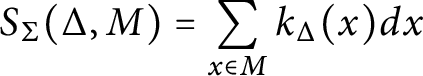 $$\begin{align*}S_{\Sigma}(\Delta, M) = \sum_{x \in M} k_\Delta(x)dx \end{align*}$$
is absolutely convergent.
Polynomiality, discrete version
The function
 $$\begin{align*}\Delta \mapsto S_{\Sigma}(\Delta, M) \end{align*}$$
is a polynomial on ${\mathcal P}(\Sigma , M)$
.
${\mathcal P}(\Sigma , M)$
.
We remark that if $K_\sigma \equiv 1$
for all nonzero cones
$K_\sigma \equiv 1$
for all nonzero cones $\sigma $
in
$\sigma $
in $\Sigma $
, then
$\Sigma $
, then $S_{\Sigma }(\Delta , M)$
coincides with the number of lattice points in
$S_{\Sigma }(\Delta , M)$
coincides with the number of lattice points in $\Delta $
. Thus, the above theorem is a far reaching generalization of the classical fact that
$\Delta $
. Thus, the above theorem is a far reaching generalization of the classical fact that $\Delta \mapsto |\Delta \cap M|$
is a polynomial function (Ehrhart polynomial; see Theorem 2.2). It is interesting to explore whether some well-known polynomials appearing in combinatorics and representation theory, e.g., in the theory of symmetric polynomials, are instances of the polynomial
$\Delta \mapsto |\Delta \cap M|$
is a polynomial function (Ehrhart polynomial; see Theorem 2.2). It is interesting to explore whether some well-known polynomials appearing in combinatorics and representation theory, e.g., in the theory of symmetric polynomials, are instances of the polynomial $J_{\Sigma }(\Delta )$
or
$J_{\Sigma }(\Delta )$
or $S_{\Sigma }(\Delta , M)$
.
$S_{\Sigma }(\Delta , M)$
.
1.6 Relation with toric varieties
Convex lattice polytopes are well studied in combinatorial algebraic geometry in relation to the geometry of toric varieties. In particular, there is a dictionary between algebraic geometric notions on toric varieties and convex geometric notions about lattice polytopes (see [Reference Cox, Little and SchenckCLS11, Reference FultonFu93]). For example, the Riemann–Roch theorem for toric varieties gives beautiful formulas relating the number of lattice points in a polytope and its volume as well as volumes of its faces (see [[Reference Brion and VergneBV97], Reference Khovanskii and PukhlikovKP93a, Reference Khovanskii and PukhlikovKP93b]).
A complete (rational) fan $\Sigma $
in
$\Sigma $
in $N_{\mathbb R}$
determines a complete toric variety
$N_{\mathbb R}$
determines a complete toric variety $X_{\Sigma }$
over
$X_{\Sigma }$
over ${\mathbb C}$
. It is an equivariant compactification of the algebraic torus
${\mathbb C}$
. It is an equivariant compactification of the algebraic torus $T_N \cong ({\mathbb C}^*)^n$
. The polytope
$T_N \cong ({\mathbb C}^*)^n$
. The polytope $\Delta \in {\mathcal P}(\Sigma )$
determines a
$\Delta \in {\mathcal P}(\Sigma )$
determines a $T_N$
-linearized ample line bundle
$T_N$
-linearized ample line bundle $\mathcal {L}_\Delta $
on
$\mathcal {L}_\Delta $
on $X_{\Sigma }$
(see Section 5).
$X_{\Sigma }$
(see Section 5).
In Section 5.2, we recall the well-known fact that the Brianchon–Gram theorem can be regarded as the computation of the equivariant Euler characteristic of an ample toric line bundle.
In Section 6, we give two interpretations of the function $k_\Delta (x)$
in terms of the toric variety
$k_\Delta (x)$
in terms of the toric variety $X_{\Sigma }$
. In Section 6.1, we interpret it as a “truncated” measure on the toric variety
$X_{\Sigma }$
. In Section 6.1, we interpret it as a “truncated” measure on the toric variety $X_{\Sigma }$
obtained by truncating a measure
$X_{\Sigma }$
obtained by truncating a measure $\omega _0$
on the open torus orbit
$\omega _0$
on the open torus orbit $X_0 \subset X_{\Sigma }$
using the measures
$X_0 \subset X_{\Sigma }$
using the measures $\omega _\sigma $
on the torus orbits
$\omega _\sigma $
on the torus orbits $O_\sigma \subset X_{\Sigma }$
(at infinity). Each tangent cone
$O_\sigma \subset X_{\Sigma }$
(at infinity). Each tangent cone $T^-_{\Delta , \sigma }$
determines an open neighborhood
$T^-_{\Delta , \sigma }$
determines an open neighborhood $\tilde {U}_{\Delta , \sigma }$
of the torus orbit closure
$\tilde {U}_{\Delta , \sigma }$
of the torus orbit closure $\overline {O}_\sigma $
. The interpretation of the tangent cones
$\overline {O}_\sigma $
. The interpretation of the tangent cones $T^-_{\Delta , \sigma }$
as neighborhoods
$T^-_{\Delta , \sigma }$
as neighborhoods $\tilde {U}_{\Delta , \sigma }$
justifies the assumption that the fan is acute: under the acute assumption, the neighborhood
$\tilde {U}_{\Delta , \sigma }$
justifies the assumption that the fan is acute: under the acute assumption, the neighborhood $\tilde {U}_{\Delta , \sigma }$
contains the orbit closure
$\tilde {U}_{\Delta , \sigma }$
contains the orbit closure $\overline {O}_\sigma $
.
$\overline {O}_\sigma $
.
In Section 6.2, we observe that computation of equivariant Euler characteristic of an ample toric line bundle has uncanny resemblances to the definition of truncated function $k_\Delta (x)$
and hence to Arthur’s construction of the modified kernel
$k_\Delta (x)$
and hence to Arthur’s construction of the modified kernel $k^T(x)$
. This leads to an interpretation of our combinatorial truncation as a Lefschetz number for computing the trace of the induced linear map of a morphism on the sheaf cohomologies of a toric variety.
$k^T(x)$
. This leads to an interpretation of our combinatorial truncation as a Lefschetz number for computing the trace of the induced linear map of a morphism on the sheaf cohomologies of a toric variety.
We point out that the similarity between the definition of $k^T(x)$
and the Brianchon–Gram theorem about polytopes has been observed by Casselman in [Reference CasselmanCass04].
$k^T(x)$
and the Brianchon–Gram theorem about polytopes has been observed by Casselman in [Reference CasselmanCass04].
The polynomiality of the number of lattice points in a polytope is related to the polynomiality of the Euler characteristic which is an immediate consequence of the Riemann–Roch theorem. From this point of view, it is probable that our Polynomiality Theorem (Theorem 4.2) is a special case of a more general Riemann–Roch-type theorem.
1.7 Relation with Arthur’s work
As we mentioned above, Arthur’s development of his noninvariant trace formula is based on the two crucial results that the integral of $k^T(x) = k^T(x,f)$
on
$k^T(x) = k^T(x,f)$
on $G({\mathbb Q}) \backslash G({\mathbb A})^1$
is absolutely convergent for
$G({\mathbb Q}) \backslash G({\mathbb A})^1$
is absolutely convergent for $T \in \mathfrak a_P^+$
sufficiently regular and
$T \in \mathfrak a_P^+$
sufficiently regular and $f \in C_c^{\infty }\left (G({\mathbb A})^1\right )$
and it is a polynomial of T. We recall that
$f \in C_c^{\infty }\left (G({\mathbb A})^1\right )$
and it is a polynomial of T. We recall that
 $$ \begin{align} k^T(x,f) = \sum\limits_P (-1)^{\dim (A_P/A_G)} \sum\limits_{\delta \in P({\mathbb Q}) \backslash G({\mathbb Q})} K_P\left(\delta x, \delta x \right) \, \widehat{\tau}_P\left(H_P(\delta x) - T \right). \end{align} $$
Here, the outer sum is over the standard parabolic subgroups P of G (containing a fixed minimal parabolic subgroup $P_0$
),
$P_0$
), $H_P : G({\mathbb A}) \longrightarrow \mathfrak a_P$
is the Harish–Chandra map, and
$H_P : G({\mathbb A}) \longrightarrow \mathfrak a_P$
is the Harish–Chandra map, and $\widehat {\tau }_P(\cdot )$
is the characteristic function of
$\widehat {\tau }_P(\cdot )$
is the characteristic function of $\left \{t \in \mathfrak a_P : \varpi (t)> 0, \varpi \in \widehat {\Delta }_P \right \}$
, where
$\left \{t \in \mathfrak a_P : \varpi (t)> 0, \varpi \in \widehat {\Delta }_P \right \}$
, where $\widehat {\Delta }_P$
consists of weights
$\widehat {\Delta }_P$
consists of weights $\varpi _\alpha $
for simple roots
$\varpi _\alpha $
for simple roots $\alpha $
corresponding to P. (We refer to [Reference ArthurAr05] for any unexplained notation.)
$\alpha $
corresponding to P. (We refer to [Reference ArthurAr05] for any unexplained notation.)
If we take $\Sigma $
to be the Weyl fan of the group G, then the parabolic subgroups of G correspond to the cones in
$\Sigma $
to be the Weyl fan of the group G, then the parabolic subgroups of G correspond to the cones in $\Sigma $
and the choice of a minimal parabolic subgroup corresponds to a choice of a full dimensional cone in
$\Sigma $
and the choice of a minimal parabolic subgroup corresponds to a choice of a full dimensional cone in $\Sigma $
with the standard parabolic subgroups corresponding to the faces of this full dimensional cone. The other cones in
$\Sigma $
with the standard parabolic subgroups corresponding to the faces of this full dimensional cone. The other cones in $\Sigma $
then correspond to the Weyl conjugates of the standard parabolic subgroups, and this correspondence between cones and parabolic subgroups is order reversing with respect to inclusion.
$\Sigma $
then correspond to the Weyl conjugates of the standard parabolic subgroups, and this correspondence between cones and parabolic subgroups is order reversing with respect to inclusion.
The Weyl fan $\Sigma $
is a full dimensional, complete, simplicial fan that satisfies the acute assumption. The toric variety
$\Sigma $
is a full dimensional, complete, simplicial fan that satisfies the acute assumption. The toric variety $X_{\Sigma }$
of the fan
$X_{\Sigma }$
of the fan $\Sigma $
is a compactification of an algebraic torus by adding strata (orbits) at infinity for each cone
$\Sigma $
is a compactification of an algebraic torus by adding strata (orbits) at infinity for each cone $\sigma \in \Sigma $
. The combinatorial truncation is an alternating sum of the
$\sigma \in \Sigma $
. The combinatorial truncation is an alternating sum of the $K_\sigma $
times the characteristic functions of certain neighborhoods of the strata at infinity.
$K_\sigma $
times the characteristic functions of certain neighborhoods of the strata at infinity.
Similarly, one has a compactification (Mumford’s toroidal compactification) of a reductive group G by adding strata $X_P$
at infinity corresponding to rational parabolic subgroups P (see [Reference Kempf, Knudsen, Mumford and Saint-DonatKKMS73, Chapter IV, Section 1]). Arthur’s truncation can be interpreted as an alternating sum of the
$X_P$
at infinity corresponding to rational parabolic subgroups P (see [Reference Kempf, Knudsen, Mumford and Saint-DonatKKMS73, Chapter IV, Section 1]). Arthur’s truncation can be interpreted as an alternating sum of the $K_P$
times characteristic functions of certain neighborhoods of the strata
$K_P$
times characteristic functions of certain neighborhoods of the strata $X_P$
at infinity.
$X_P$
at infinity.
The similarity between (1.2) and (1.3) is clear. This suggests that there is a corresponding family of functions $(K_\sigma )_{\sigma \in \Sigma }$
defined using the
$(K_\sigma )_{\sigma \in \Sigma }$
defined using the $K_P$
functions. We believe that our combinatorial arguments, or a variant thereof, can be used to give convergence and polynomiality results of Arthur as follows. One would use the analytic arguments already in Arthur’s work to verify the assumptions of (the variant of) our convergence and polynomiality theorems. As a consequence, one would recover Arthur’s results making the combinatorial/geometric ingredients of his proofs more streamlined, at least in our view.
$K_P$
functions. We believe that our combinatorial arguments, or a variant thereof, can be used to give convergence and polynomiality results of Arthur as follows. One would use the analytic arguments already in Arthur’s work to verify the assumptions of (the variant of) our convergence and polynomiality theorems. As a consequence, one would recover Arthur’s results making the combinatorial/geometric ingredients of his proofs more streamlined, at least in our view.
We expect that one can extend the geometric interpretations of truncation (e.g., as a Lefschetz number) in Section 6 to Arthur’s setup by replacing the toric variety $X_{\Sigma }$
by Mumford’s toroidal compactification of a reductive algebraic group G. We hope to write the details, using Reduction Theory, in our next paper on this subject.
$X_{\Sigma }$
by Mumford’s toroidal compactification of a reductive algebraic group G. We hope to write the details, using Reduction Theory, in our next paper on this subject.
2 Preliminaries
We review some basic notions from the theory of polyhedral cones and fix some notations along the way. We refer to [Reference Cox, Little and SchenckCLS11, Section 1.2] for further details.
2.1 Cones and fans
Let V be a finite dimensional real vector space of dimension n, and let $V^*$
denote its dual. Recall that a (closed convex) polyhedral cone in V is a set of the form
$V^*$
denote its dual. Recall that a (closed convex) polyhedral cone in V is a set of the form
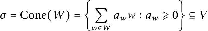 $$\begin{align*}\sigma = \operatorname{Cone}(W) = \left\{ \sum\limits_{w \in W} a_w w : a_w \geqslant 0 \right\} \subseteq V \end{align*}$$
with W a finite subset of V. Equivalently, there is a finite subset B of $V^*$
such that
$V^*$
such that
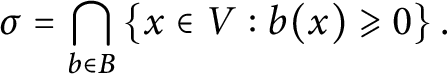 $$\begin{align*}\sigma = \bigcap\limits_{b \in B} \left\{x \in V : b(x) \geqslant 0 \right\}. \end{align*}$$
We say that $\sigma $
is generated by W. Also, we write
$\sigma $
is generated by W. Also, we write $\operatorname {Cone}(\emptyset ) = \{0\}$
. The dimension of
$\operatorname {Cone}(\emptyset ) = \{0\}$
. The dimension of $\sigma $
is the dimension of its linear span. The dual cone
$\sigma $
is the dimension of its linear span. The dual cone $\sigma ^\vee $
is defined as
$\sigma ^\vee $
is defined as
 $$\begin{align*}\sigma^\vee := \left\{ y \in V^* : y(x) \geqslant 0 \mbox{ for all } x \in \sigma\right\}. \end{align*}$$
Dual cones enjoy the property that if $\sigma $
is a polyhedral cone in V, then
$\sigma $
is a polyhedral cone in V, then $\sigma ^\vee $
is a polyhedral cone in
$\sigma ^\vee $
is a polyhedral cone in $V^*$
and
$V^*$
and $\sigma ^{\vee \vee } = \sigma $
.
$\sigma ^{\vee \vee } = \sigma $
.
For a face $\tau $
of
$\tau $
of $\sigma $
(denoted
$\sigma $
(denoted $\tau \preceq \sigma $
), define its dual face
$\tau \preceq \sigma $
), define its dual face
 $$ \begin{align*} \tau^* &= \left\{y \in \sigma^\vee : y(x) = 0 \mbox{ for all } x\in\tau \right\} \\ &= \sigma^\vee \cap \tau^\perp. \end{align*} $$
Then $\tau ^*$
is a face of
$\tau ^*$
is a face of $\sigma ^\vee $
,
$\sigma ^\vee $
, $\tau ^{**} = \tau $
,
$\tau ^{**} = \tau $
, $\tau \leftrightarrow \tau ^*$
is an inclusion-reversing bijection between faces of
$\tau \leftrightarrow \tau ^*$
is an inclusion-reversing bijection between faces of $\sigma $
and those of
$\sigma $
and those of $\sigma ^\vee $
, and
$\sigma ^\vee $
, and $\dim \tau + \dim \tau ^* = n$
. One-dimensional cones, i.e., half-lines, are called rays. A face
$\dim \tau + \dim \tau ^* = n$
. One-dimensional cones, i.e., half-lines, are called rays. A face $\tau $
of
$\tau $
of $\sigma $
is called a facet if
$\sigma $
is called a facet if $\dim \tau = \dim \sigma - 1$
, and its linear span is referred to as a wall of
$\dim \tau = \dim \sigma - 1$
, and its linear span is referred to as a wall of $\sigma $
. An edge is a face of dimension 1.
$\sigma $
. An edge is a face of dimension 1.
Define the relative interior $\sigma ^\circ $
of
$\sigma ^\circ $
of $\sigma $
to be the interior of
$\sigma $
to be the interior of $\sigma $
in its span. One then checks that
$\sigma $
in its span. One then checks that $x \in \sigma ^\circ $
if and only if
$x \in \sigma ^\circ $
if and only if $y(x)> 0$
for all
$y(x)> 0$
for all $y \in \sigma ^\vee \setminus \sigma ^\perp $
. A polyhedral cone
$y \in \sigma ^\vee \setminus \sigma ^\perp $
. A polyhedral cone $\sigma $
in V is strongly convex if the origin is a face. This is the case if and only if
$\sigma $
in V is strongly convex if the origin is a face. This is the case if and only if $\sigma $
contains no positive dimensional subspace of V if and only if
$\sigma $
contains no positive dimensional subspace of V if and only if $\sigma \cap (-\sigma ) = \{0\}$
if and only if
$\sigma \cap (-\sigma ) = \{0\}$
if and only if $\dim \sigma ^\vee = n$
. A strongly convex polyhedral cone
$\dim \sigma ^\vee = n$
. A strongly convex polyhedral cone $\sigma \subseteq V$
is called simplicial if it is generated by linearly independent vectors. We note that the dual of a simplicial cone of maximal dimension is again simplicial.
$\sigma \subseteq V$
is called simplicial if it is generated by linearly independent vectors. We note that the dual of a simplicial cone of maximal dimension is again simplicial.
For $y \in V^*$
, we set
$y \in V^*$
, we set
 $$\begin{align*}H_y := \left\{x \in V : y(x) = 0 \right\} \subseteq V \end{align*}$$
and define the closed (resp. open) spaces
 $$\begin{align*}H^+_y := \left\{x \in V : y(x) \geqslant 0 \right\} \subseteq V \quad \mbox{ and } \quad H^-_y := \left\{x \in V : y(x) < 0 \right\} \subseteq V. \end{align*}$$
When $y \not = 0, \ H_y$
is a hyperplane and
$y \not = 0, \ H_y$
is a hyperplane and $H^+_y$
and
$H^+_y$
and $H^-_y$
are half-spaces in V. When
$H^-_y$
are half-spaces in V. When $y=0$
, we have
$y=0$
, we have $H_y = H^+_y = V$
while
$H_y = H^+_y = V$
while $H_y^-$
is empty. If
$H_y^-$
is empty. If $\sigma \subseteq H^+_y$
for
$\sigma \subseteq H^+_y$
for $y \not = 0$
, we say
$y \not = 0$
, we say $H_y$
is a supporting hyperplane and
$H_y$
is a supporting hyperplane and $H^+_y$
(resp.
$H^+_y$
(resp. $H^-_y$
) is an inward (resp. outward) supporting half-space of
$H^-_y$
) is an inward (resp. outward) supporting half-space of $\sigma $
. (When
$\sigma $
. (When $y=0$
, we automatically have
$y=0$
, we automatically have $\sigma \subseteq H^+_0 = H_0 = V$
.) Note that
$\sigma \subseteq H^+_0 = H_0 = V$
.) Note that $H_y$
is a supporting hyperplane of
$H_y$
is a supporting hyperplane of $\sigma $
if and only if
$\sigma $
if and only if $y \in \sigma ^\vee \setminus \{0\}$
. If
$y \in \sigma ^\vee \setminus \{0\}$
. If $y_1, y_2, \dots , y_r$
generate
$y_1, y_2, \dots , y_r$
generate $\sigma ^\vee ,$
then
$\sigma ^\vee ,$
then $\sigma = H^+_{y_1} \cap \cdots \cap H^+_{y_r}$
. Thus, every polyhedral cone is an intersection of finitely many closed half-spaces.
$\sigma = H^+_{y_1} \cap \cdots \cap H^+_{y_r}$
. Thus, every polyhedral cone is an intersection of finitely many closed half-spaces.
A fan $\Sigma $
in V is a finite collection of cones
$\Sigma $
in V is a finite collection of cones $\sigma \subseteq V$
satisfying the following three properties: (a) every
$\sigma \subseteq V$
satisfying the following three properties: (a) every $\sigma \in \Sigma $
is a strongly convex polyhedral cone, (b) for all
$\sigma \in \Sigma $
is a strongly convex polyhedral cone, (b) for all $\sigma \in \Sigma ,$
each face of
$\sigma \in \Sigma ,$
each face of $\sigma $
also belongs to
$\sigma $
also belongs to $\Sigma $
, and (c) for all
$\Sigma $
, and (c) for all $\sigma _1, \sigma _2 \in \Sigma $
, the intersection
$\sigma _1, \sigma _2 \in \Sigma $
, the intersection $\sigma _1 \cap \sigma _2$
is a face of each. The set of r-dimensional cones of
$\sigma _1 \cap \sigma _2$
is a face of each. The set of r-dimensional cones of $\Sigma $
is denoted by
$\Sigma $
is denoted by $\Sigma (r)$
. The support of
$\Sigma (r)$
. The support of $\Sigma $
is defined by
$\Sigma $
is defined by
 $$\begin{align*}|\Sigma| := \bigcup_{\sigma \in \Sigma} \, \sigma \subseteq V. \end{align*}$$
If $|\Sigma | = V$
, then
$|\Sigma | = V$
, then $\Sigma $
is called a complete fan. A simplicial fan is a fan all whose cones are simplicial. Every fan can be refined into a simplicial fan.
$\Sigma $
is called a complete fan. A simplicial fan is a fan all whose cones are simplicial. Every fan can be refined into a simplicial fan.
Finally, for $\sigma \in \Sigma $
, we let
$\sigma \in \Sigma $
, we let $\Sigma / \sigma $
denote the fan in
$\Sigma / \sigma $
denote the fan in $V / \operatorname {Span}(\sigma )$
consisting of all the images of the cones
$V / \operatorname {Span}(\sigma )$
consisting of all the images of the cones $\sigma ' \succeq \sigma $
. If we fix an inner product on V, then
$\sigma ' \succeq \sigma $
. If we fix an inner product on V, then $V / \operatorname {Span}(\sigma )$
can be identified with
$V / \operatorname {Span}(\sigma )$
can be identified with $\sigma ^\perp $
and
$\sigma ^\perp $
and $\Sigma / \sigma $
consists of projections of
$\Sigma / \sigma $
consists of projections of $\sigma ' \succeq \sigma $
onto
$\sigma ' \succeq \sigma $
onto $\sigma ^\perp $
.
$\sigma ^\perp $
.
2.2 Polytopes
A polytope is a set in $V^*$
of the form
$V^*$
of the form
 $$\begin{align*}P = \operatorname{Conv}(S) = \left\{ \sum\limits_{u \in S} \lambda_u u : \lambda_u \geqslant 0, \sum_{u \in S} \lambda_u = 1 \right\}, \end{align*}$$
where S is a finite subset of $V^*$
. We say P is the convex hull of S. The dimension,
$V^*$
. We say P is the convex hull of S. The dimension, $\dim P$
, of a polytope P is the dimension of the smallest affine subspace of
$\dim P$
, of a polytope P is the dimension of the smallest affine subspace of $V^*$
containing P. Given
$V^*$
containing P. Given $x \in V \setminus \{0\}$
and
$x \in V \setminus \{0\}$
and $r \in {\mathbb R}$
, we have the affine hyperplane
$r \in {\mathbb R}$
, we have the affine hyperplane
 $$\begin{align*}H_{x,r} := \left\{ y \in V^* : y(x) = r \right\} \end{align*}$$
and the closed (resp. open) half-spaces
 $$\begin{align*}H_{x,r}^{+} := \left\{ y \in V^* : y(x) \geqslant r \right\} \quad \mbox{ and } \quad H_{x,r}^{-} := \left\{ y \in V^* : y(x) < r \right\}. \end{align*}$$
A subset $Q \subseteq P$
is a face of P, denoted by
$Q \subseteq P$
is a face of P, denoted by $Q \preceq P$
, if there is
$Q \preceq P$
, if there is $x \in V \setminus \{0\}$
and there is
$x \in V \setminus \{0\}$
and there is $r \in {\mathbb R}$
with
$r \in {\mathbb R}$
with
 $$\begin{align*}Q = H_{x,r} \cap P \quad\mbox{ and }\quad P \subseteq H_{x,r}^+. \end{align*}$$
We then say that $H_{x,r}$
is a supporting affine hyperplane. The polytope P is regarded as a face of itself and faces of P of dimensions
$H_{x,r}$
is a supporting affine hyperplane. The polytope P is regarded as a face of itself and faces of P of dimensions $0$
,
$0$
, $1$
, and
$1$
, and $(\dim P - 1)$
are called vertices, edges, and facets, respectively.
$(\dim P - 1)$
are called vertices, edges, and facets, respectively.
A polytope $P \subseteq V^*$
can be written as a finite intersection of closed half-spaces, and an intersection
$P \subseteq V^*$
can be written as a finite intersection of closed half-spaces, and an intersection
 $$\begin{align*}P = \bigcap\limits_{i=1}^s H_{x_i,r_i}^+ \end{align*}$$
is a polytope provided that it is bounded. In general, an intersection of finitely many closed half-spaces is called a polyhedron and could be unbounded. When $\dim P = \dim V^*$
(i.e., full dimensional polytope) for each facet F, we have a unique supporting affine hyperplane and the corresponding closed half-space given by
$\dim P = \dim V^*$
(i.e., full dimensional polytope) for each facet F, we have a unique supporting affine hyperplane and the corresponding closed half-space given by
 $$\begin{align*}H_F = H_{u_F^+,a_F} = \left\{ y \in V^* : y(u^+_F) = a_F \right\} \end{align*}$$
and
 $$\begin{align*}H_F^{+} = H^+_{u_F^+,a_F} = \left\{ y \in V^* : y(u^+_F) \geqslant a_F \right\}, \end{align*}$$
where $(u^+_F, a_F) \in V \times {\mathbb R}$
is unique up to multiplication by a positive real number. We call
$(u^+_F, a_F) \in V \times {\mathbb R}$
is unique up to multiplication by a positive real number. We call $u^+_F$
an inward-pointing facet normal of the facet F. Hence,
$u^+_F$
an inward-pointing facet normal of the facet F. Hence,
 $$ \begin{align} P = \bigcap\limits_{F \text{ facet }} H_F^+ = \left\{ y \in V^* : y(u^+_F) \geqslant a_F \mbox{ for all proper facets } F \prec P \right\}. \end{align} $$
This is the so-called facet representation of P. We also have a similar representation with outward-pointing facet normals $u^-_F = - u^+_F$
. When the facet normals
$u^-_F = - u^+_F$
. When the facet normals $u^{\pm }_F$
are assumed to be unit vectors, we may call the
$u^{\pm }_F$
are assumed to be unit vectors, we may call the $a_F$
the support numbers of P.
$a_F$
the support numbers of P.
Let Q be a face of P and define the inward (resp. outward) tangent cone $T^+_{P, Q}$
(resp.
$T^+_{P, Q}$
(resp. $T^-_{P, Q}$
) via
$T^-_{P, Q}$
) via
 $$ \begin{align} \phantom{\text{resp.~\, }}T^+_{P, Q} &:= \left\{ y \in V^* : y(u^+_F) \geqslant a_F \mbox{ for all facets } F \supset Q \right\}, \end{align} $$
 $$ \begin{align} \text{resp. } T^-_{P, Q}&:=\left\{ y \in V^* : y(u^+_F) < a_F \mbox{ for all facets } F \supset Q \right\} \end{align} $$
 $$\begin{align*}&\phantom{\text{resp.~\, QP~~~}}= \left\{ y \in V^* : y(u^-_F)> a_F \mbox{ for all facets } F \supset Q \right\}. \notag \end{align*}$$
See Figures 3 and 4 for illustrations of inward and outward tangent cones of a quadrilateral at a vertex and at an edge, respectively.
A polytope $P \subseteq V^*$
of dimension d is called a d-simplex (or just a simplex) if it has
$P \subseteq V^*$
of dimension d is called a d-simplex (or just a simplex) if it has $d+1$
vertices, simplicial if every facet is a simplex, and simple if every vertex is the intersection of precisely d facets.
$d+1$
vertices, simplicial if every facet is a simplex, and simple if every vertex is the intersection of precisely d facets.
Given a polytope $P = \operatorname {Conv}(S)$
, its multiple
$P = \operatorname {Conv}(S)$
, its multiple $rP = \operatorname {Conv}(rS)$
is also a polytope for any
$rP = \operatorname {Conv}(rS)$
is also a polytope for any $r \geqslant 0$
. The Minkowski sum
$r \geqslant 0$
. The Minkowski sum $P_1 + P_2 = \{y_1+y_2 : y_i \in P_i\}$
of two polytopes
$P_1 + P_2 = \{y_1+y_2 : y_i \in P_i\}$
of two polytopes $P_1 = \operatorname {Conv}(S_1)$
and
$P_1 = \operatorname {Conv}(S_1)$
and $P_2 = \operatorname {Conv}(S_2)$
is again a polytope, and we have the distributive law
$P_2 = \operatorname {Conv}(S_2)$
is again a polytope, and we have the distributive law $rP + sP = (r+s) P$
. The set
$rP + sP = (r+s) P$
. The set $\mathcal {P}(V^*)$
of polytopes in
$\mathcal {P}(V^*)$
of polytopes in $V^*$
together with the Minkowski sum is a cancellative semigroup. The following theorem is originally due to Minkowski.
$V^*$
together with the Minkowski sum is a cancellative semigroup. The following theorem is originally due to Minkowski.
Theorem 2.1 (Volume polynomial)
The map $P \mapsto \operatorname {vol}_n(P)$
is a polynomial function on
$P \mapsto \operatorname {vol}_n(P)$
is a polynomial function on ${\mathcal P}(V^*)$
in the following sense: let
${\mathcal P}(V^*)$
in the following sense: let $P_1, \ldots , P_r$
be polytopes in
$P_1, \ldots , P_r$
be polytopes in $V^*$
. For any
$V^*$
. For any $\lambda _1, \ldots , \lambda _r \geqslant 0$
, we can form the polytope
$\lambda _1, \ldots , \lambda _r \geqslant 0$
, we can form the polytope $\sum _i \lambda _i P_i$
. Then the function
$\sum _i \lambda _i P_i$
. Then the function $(\lambda _1, \ldots , \lambda _r) \mapsto \operatorname {vol}_n(\sum _i \lambda _i P_i)$
is the restriction of a homogeneous polynomial on
$(\lambda _1, \ldots , \lambda _r) \mapsto \operatorname {vol}_n(\sum _i \lambda _i P_i)$
is the restriction of a homogeneous polynomial on ${\mathbb R}^r$
to the positive orthant
${\mathbb R}^r$
to the positive orthant ${\mathbb R}_{\geqslant 0}^r$
.
${\mathbb R}_{\geqslant 0}^r$
.
There is also a discrete analogue of Theorem 2.1 which is harder and more subtle to prove. It is a generalization of the notion of the Ehrhart polynomial. Let $M \cong {\mathbb Z}^n$
be a full rank lattice in
$M \cong {\mathbb Z}^n$
be a full rank lattice in $V^* \cong {\mathbb R}^n$
. Let
$V^* \cong {\mathbb R}^n$
. Let ${\mathcal P}(M)$
denote the collection of lattice polytopes with respect to M, that is, all polytopes in
${\mathcal P}(M)$
denote the collection of lattice polytopes with respect to M, that is, all polytopes in $V^*$
whose vertices belong to M. The set
$V^*$
whose vertices belong to M. The set ${\mathcal P}(M)$
is closed under the Minkowski sum and multiplication by positive integers.
${\mathcal P}(M)$
is closed under the Minkowski sum and multiplication by positive integers.
Theorem 2.2 (Ehrhart polynomial)
The map $P \mapsto |P \cap M|$
is a polynomial map on
$P \mapsto |P \cap M|$
is a polynomial map on ${\mathcal P}(M)$
.
${\mathcal P}(M)$
.
More generally, the polynomiality property holds for any valuation (also called finitely additive measure). A function $\Phi : {\mathcal P}(M) \to {\mathbb R}_{\geqslant 0}$
is called a valuation if for all
$\Phi : {\mathcal P}(M) \to {\mathbb R}_{\geqslant 0}$
is called a valuation if for all $P_1, P_2 \in {\mathcal P}(M)$
, the following hold:
$P_1, P_2 \in {\mathcal P}(M)$
, the following hold:
-
(1)
$\Phi $
is monotone with respect to inclusion, i.e.,
$\Phi (P_1) \leq \Phi (P_2)$
provided that
$P_1 \subset P_2$
. -
(2)
$\Phi (P_1 \cup P_2) = \Phi (P_1) + \Phi (P_2) - \Phi (P_1 \cap P_2)$
.


We say $\Phi $
is
$\Phi $
is ${{\mathbb Z}}^n$
-invariant if
${{\mathbb Z}}^n$
-invariant if $\Phi (m+P) = \Phi (P)$
for all
$\Phi (m+P) = \Phi (P)$
for all $P \in {\mathcal P}(M)$
and
$P \in {\mathcal P}(M)$
and $m \in M$
. The following is a beautiful result of McMullen [Reference McMullenMc77]. It generalizes Theorem 2.2.
$m \in M$
. The following is a beautiful result of McMullen [Reference McMullenMc77]. It generalizes Theorem 2.2.
Theorem 2.3 Let $\Phi $
be a
$\Phi $
be a ${\mathbb Z}^n$
-invariant valuation on
${\mathbb Z}^n$
-invariant valuation on ${\mathcal P}(M)$
. Then
${\mathcal P}(M)$
. Then $\Phi $
is a polynomial function.
$\Phi $
is a polynomial function.


2.3 Normal fan
For $Q \preceq P$
, let
$Q \preceq P$
, let
 $$\begin{align*}\sigma_Q := \operatorname{Cone}\left( u^-_F : \text{ facets } F \supset Q \right). \end{align*}$$
Given a full dimensional polytope $P \subseteq V^*$
, the cones
$P \subseteq V^*$
, the cones $\sigma _Q$
fit together to form the normal fan of P in V given by
$\sigma _Q$
fit together to form the normal fan of P in V given by
 $$\begin{align*}\Sigma_P = \left\{ \sigma_Q : Q \preceq P \right\}. \end{align*}$$
Note that we have used outward facet normals $u^-_F$
to define the normal fan (see Figure 5). (Some authors use inward facet normals
$u^-_F$
to define the normal fan (see Figure 5). (Some authors use inward facet normals $u^+_F$
instead.)
$u^+_F$
instead.)
A polygon and its normal fan. Note that in our convention, we use outward facet normals to define the cones in the normal fan.

Let $\mathcal {P}(\Sigma )$
be the collection of all convex polytopes whose normal fan is
$\mathcal {P}(\Sigma )$
be the collection of all convex polytopes whose normal fan is $\Sigma $
. This set is closed under the Minkowski sum of polytopes and multiplication by positive scalars. For
$\Sigma $
. This set is closed under the Minkowski sum of polytopes and multiplication by positive scalars. For $P \in \mathcal {P}(\Sigma )$
, we have an inclusion-reversing bijection
$P \in \mathcal {P}(\Sigma )$
, we have an inclusion-reversing bijection
 $$ \begin{align} Q = Q_\sigma \longleftrightarrow \sigma = \sigma_Q \end{align} $$
between the set of faces of P and the set of cones in the normal fan $\Sigma $
. In particular, the facets F of P correspond to rays
$\Sigma $
. In particular, the facets F of P correspond to rays $\rho \in \Sigma (1)$
. For a ray
$\rho \in \Sigma (1)$
. For a ray $\rho \in \Sigma (1)$
, we set
$\rho \in \Sigma (1)$
, we set $a_\rho = a_F$
, where F is the facet corresponding to
$a_\rho = a_F$
, where F is the facet corresponding to $\rho $
and
$\rho $
and $a_F$
are the support numbers of P (see (2.1)). The map
$a_F$
are the support numbers of P (see (2.1)). The map $P \mapsto (a_\rho )_{\rho \in \Sigma (1)}$
gives an embedding of
$P \mapsto (a_\rho )_{\rho \in \Sigma (1)}$
gives an embedding of $\mathcal {P}(\Sigma )$
into
$\mathcal {P}(\Sigma )$
into ${\mathbb R}^s$
, where
${\mathbb R}^s$
, where $s=|\Sigma (1)|$
. The image is a full dimensional (open) convex polyhedral cone.
$s=|\Sigma (1)|$
. The image is a full dimensional (open) convex polyhedral cone.
Let P be a full dimensional polytope with normal fan $\Sigma _P$
. Let
$\Sigma _P$
. Let $Q \preceq P$
be a face with corresponding cone
$Q \preceq P$
be a face with corresponding cone $\sigma _Q \in \Sigma _P$
. Then the normal fan
$\sigma _Q \in \Sigma _P$
. Then the normal fan $\Sigma _Q$
(of the polytope Q) is the fan
$\Sigma _Q$
(of the polytope Q) is the fan $\Sigma _P / \sigma _Q$
(defined at the end of Section 2.1). It consists of the images of the cones
$\Sigma _P / \sigma _Q$
(defined at the end of Section 2.1). It consists of the images of the cones $\sigma ' \succeq \sigma _Q$
in the quotient vector space
$\sigma ' \succeq \sigma _Q$
in the quotient vector space $V / \operatorname {Span}(\sigma _Q)$
.
$V / \operatorname {Span}(\sigma _Q)$
.
2.4 Nearest face partition
Fix an inner product $\langle \cdot , \cdot \rangle $
on V. Let
$\langle \cdot , \cdot \rangle $
on V. Let $P \subset V$
be a convex polyhedron. To P, we can associate a partition of V into polyhedral regions
$P \subset V$
be a convex polyhedron. To P, we can associate a partition of V into polyhedral regions $V_P^Q$
as follows. For each face
$V_P^Q$
as follows. For each face $Q \preceq P$
, let
$Q \preceq P$
, let
 $$ \begin{align*}V_P^Q &= \left\{ x \in V : \text{the minimum distance from } x \text{ to } P \text{ is attained}\right. \\&\qquad \left.\text{at a point in the relative interior of } Q \right\}.\end{align*} $$
The following is straightforward to verify.
Proposition 2.5
-
(1) For each face
$Q \preceq P$
, the set
$V_P^Q$
is a polyhedron. -
(2) We have a disjoint union
$$\begin{align*}V = \bigsqcup\limits_{Q \preceq P} V_P^Q. \end{align*}$$


We can modify the $V_P^Q$
to obtain a slightly different partition
$V_P^Q$
to obtain a slightly different partition $\left \{W_P^Q : Q \preceq P \right \}$
. For each face
$\left \{W_P^Q : Q \preceq P \right \}$
. For each face $Q \preceq P$
, let
$Q \preceq P$
, let
 $$ \begin{align*}W_P^Q = \overline{V_P^Q} \setminus \bigg(\bigcup_{Q' \gneqq Q} \overline{V_P^{Q'}}\bigg),\end{align*} $$
where $\overline {V_P^Q}$
denotes the closure of
$\overline {V_P^Q}$
denotes the closure of $V_P^Q$
. The polyhedra
$V_P^Q$
. The polyhedra $W_P^Q$
and
$W_P^Q$
and $V_P^Q$
have the same relative interior, but they are different on the boundary.
$V_P^Q$
have the same relative interior, but they are different on the boundary.
We refer to both $\left \{V_P^Q : Q \preceq P \right \}$
and
$\left \{V_P^Q : Q \preceq P \right \}$
and $\left \{W_P^Q : Q \preceq P \right \}$
as the nearest face partition of V with respect to the polyhedron P (see Figure 6). We note that if, in particular,
$\left \{W_P^Q : Q \preceq P \right \}$
as the nearest face partition of V with respect to the polyhedron P (see Figure 6). We note that if, in particular, $P = \sigma $
is a cone (with apex at the origin), then the closure of the parts in the partition with respect to
$P = \sigma $
is a cone (with apex at the origin), then the closure of the parts in the partition with respect to $\sigma $
in fact form a complete fan in V. In practice, we will also use the nearest face partition to partition a polyhedron inside V.
$\sigma $
in fact form a complete fan in V. In practice, we will also use the nearest face partition to partition a polyhedron inside V.
Nearest face partition for a polygon illustrating polyhedral regions $V_P^Q$
and
$V_P^Q$
and $W_P^Q$
corresponding to an edge Q.
$W_P^Q$
corresponding to an edge Q.
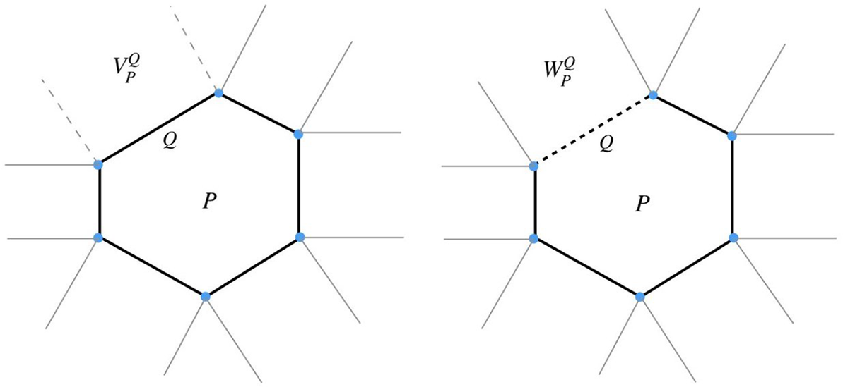
2.5 Conical decomposition theorems
We end this section by recalling two beautiful formulas which represent the characteristic function of a polytope as an alternating sum of characteristic functions of cones. For a nice overview of these decompositions and related topics, we refer the reader to [Reference Beck, Haase and SottileBHS09].
2.5.1 Brianchon–Gram theorem
The first conical decomposition theorem we discuss is the Brianchon–Gram theorem. It is named after Brianchon and Gram who independently proved the $n = 3$
case in 1837 and 1874, respectively ([Reference BrianchonB37, Reference GramG1874]). It is the mother of all cone decompositions! See [Reference HaaseHass05, Section 1.1] and the references therein. Also, see [Reference AgapitoAg06].
$n = 3$
case in 1837 and 1874, respectively ([Reference BrianchonB37, Reference GramG1874]). It is the mother of all cone decompositions! See [Reference HaaseHass05, Section 1.1] and the references therein. Also, see [Reference AgapitoAg06].
Theorem 2.6 (Brianchon–Gram)
Let P be a polytope in $V^*$
. We have the following equality, where
$V^*$
. We have the following equality, where ${\textbf 1}$
denotes characteristic function:
${\textbf 1}$
denotes characteristic function:
 $$ \begin{align} {{\textbf 1}}_P = \sum_{Q \preceq P} (-1)^{\dim Q} {{\textbf 1}}_{T^+_{P, Q}}. \end{align} $$
Proof For a point $y \in P$
, the right-hand side computes the Euler characteristic of P and hence is equal to
$y \in P$
, the right-hand side computes the Euler characteristic of P and hence is equal to $1$
since P is contractible. For
$1$
since P is contractible. For $y \notin P$
, we have to subtract the Euler characteristic of the subcomplex that is visible from y which is again contractible.▪
$y \notin P$
, we have to subtract the Euler characteristic of the subcomplex that is visible from y which is again contractible.▪
Alternatively, one can formulate Brianchon–Gram in terms of outward-looking tangent cones.
Theorem 2.7 (Brianchon–Gram, alternative version)
Let P be a polytope in $V^*$
. We have the following equality:
$V^*$
. We have the following equality:
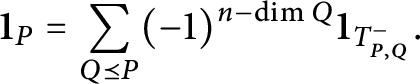 $$ \begin{align} {{\textbf 1}}_{P} = \sum_{Q \preceq P} (-1)^{n - \dim Q} {{\textbf 1}}_{T^-_{P, Q}}. \end{align} $$
The above version of the Brianchon–Gram formula looks similar to Arthur’s definition of the modified kernel $k^T(x)$
, as was observed in [Reference CasselmanCass04]. See Figures 7 and 8 for illustrations of (2.5) and (2.6).
$k^T(x)$
, as was observed in [Reference CasselmanCass04]. See Figures 7 and 8 for illustrations of (2.5) and (2.6).
Illustration of the Brianchon–Gram theorem (inward-looking tangent cones) for a triangle.
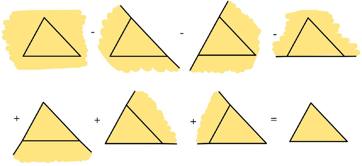
Illustration of the Brianchon–Gram theorem (alternative version, outward-looking tangent cones) for a triangle.
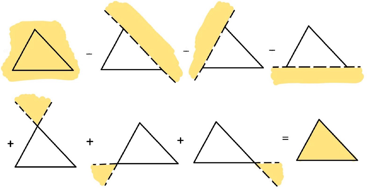
2.5.2 Lawrence–Varchenko theorem
The second conical decomposition due to Lawrence [Reference LawrenceLaw91] and Varchenko [Reference VarchenkoVr87] represents the characteristic function of a polytope as an alternating sum of characteristic functions of certain cones associated with vertices of the polytope. It is a predecessor to the work of Khovanskii and Pukhlikov [Reference Khovanskii and PukhlikovKP93a, Reference Khovanskii and PukhlikovKP93b] and Brion and Vergne [Reference BrionBr88, Reference Brion and VergneBV97]. It is related to Morse theory on polytopes as well as equivariant cohomology of toric varieties. The Lawrence–Varchenko theorem follows immediately from Khovanskii–Pukhlikov results as well (see [Reference Khovanskii and PukhlikovKP93b, Section 3.2]).
Let $P \subset V$
be a simple polytope, and let v be a vertex of P. Let
$P \subset V$
be a simple polytope, and let v be a vertex of P. Let $w_1, \ldots w_r$
be edge vectors of P at the vertex v. Fix a dual vector
$w_1, \ldots w_r$
be edge vectors of P at the vertex v. Fix a dual vector $\xi \in V^*$
such that
$\xi \in V^*$
such that $\langle w_i, \xi \rangle \neq 0$
, for all i. We define vectors
$\langle w_i, \xi \rangle \neq 0$
, for all i. We define vectors $w^{\prime }_1, \ldots , w^{\prime }_r$
as follows:
$w^{\prime }_1, \ldots , w^{\prime }_r$
as follows:
 $$ \begin{align*} w^{\prime}_i = \begin{cases} w_i, & \mbox{ if } \langle w_i, \xi \rangle> 0, \\ - w_i, & \mbox{ otherwise. } \end{cases} \end{align*} $$
Finally, define the polarized tangent cone $T^\xi _{P, v}$
with apex at v by
$T^\xi _{P, v}$
with apex at v by
 $$\begin{align*}T^\xi_{P, v} = \left\{ \sum_{i=1}^r \lambda_i w^{\prime}_i : \begin{array}{ll} \lambda_i \geqslant 0 \text{ if } w^{\prime}_i = w_i \\ \lambda_i> 0 \text{ if } w^{\prime}_i = -w_i \end{array} \right\}. \end{align*}$$
Theorem 2.8 (Lawrence–Varchenko)
With notation as above, we have the following:
 $$ \begin{align} {\textbf 1}_P = \sum_{v} (-1)^{n_v} {\textbf 1}_{T^\xi_{P, v}}, \end{align} $$
where the sum is over all the vertices v of P, and $n_v = |\{i : w^{\prime }_i = -w_i \}|$
.
$n_v = |\{i : w^{\prime }_i = -w_i \}|$
.
See Figure 9 for an illustration of (2.7).
Illustration of the Lawrence–Varchenko theorem for a quadrangle.

2.6 Khovanskii–Pukhlikov virtual polytopes and convex chains
This is a summary of some ideas and results from [Reference Khovanskii and PukhlikovKP93a, Reference Khovanskii and PukhlikovKP93b] that we will need later. As before, $V \cong {\mathbb R}^n$
denotes an n-dimensional real vector space.
$V \cong {\mathbb R}^n$
denotes an n-dimensional real vector space.
Recall that ${\mathcal P}(V^*)$
denotes the set of polytopes in the dual space
${\mathcal P}(V^*)$
denotes the set of polytopes in the dual space $V^*$
. The set
$V^*$
. The set $\mathcal {P}(V^*)$
is equipped with the operations of Minkowski sum and multiplication by positive scalars. One knows that
$\mathcal {P}(V^*)$
is equipped with the operations of Minkowski sum and multiplication by positive scalars. One knows that ${\mathcal P}(V^*)$
together with the Minkowski sum is a cancellative semigroup and hence it can be extended to a real vector space
${\mathcal P}(V^*)$
together with the Minkowski sum is a cancellative semigroup and hence it can be extended to a real vector space $\mathcal {V}(V^*)$
consisting of formal differences
$\mathcal {V}(V^*)$
consisting of formal differences $P_1 - P_2$
,
$P_1 - P_2$
, $P_i \in \mathcal {P}(V^*)$
, where for polytopes
$P_i \in \mathcal {P}(V^*)$
, where for polytopes $P_1, P_2, P^{\prime }_1, P^{\prime }_2$
, we have
$P_1, P_2, P^{\prime }_1, P^{\prime }_2$
, we have $P_1 - P_2 = P^{\prime }_1 - P^{\prime }_2$
if and only if
$P_1 - P_2 = P^{\prime }_1 - P^{\prime }_2$
if and only if $P_1 + P^{\prime }_2 = P^{\prime }_1 + P_2$
.
$P_1 + P^{\prime }_2 = P^{\prime }_1 + P_2$
.
Definition 2.1 (Virtual polytope)
The elements of $\mathcal {V}(V^*)$
are called virtual polytopes (see [Reference Khovanskii and PukhlikovKP93a]).
$\mathcal {V}(V^*)$
are called virtual polytopes (see [Reference Khovanskii and PukhlikovKP93a]).
We note that ${\mathcal V}(V^*)$
is an infinite dimensional vector space.
${\mathcal V}(V^*)$
is an infinite dimensional vector space.
Let $\Sigma $
be a complete fan in V. Recall that
$\Sigma $
be a complete fan in V. Recall that ${\mathcal P}(\Sigma )$
denotes the set of all polytopes in
${\mathcal P}(\Sigma )$
denotes the set of all polytopes in $V^*$
whose normal fan is
$V^*$
whose normal fan is $\Sigma $
. The set
$\Sigma $
. The set ${\mathcal P}(\Sigma )$
is closed under the Minkowski sum and multiplication by positive scalars. We denote by
${\mathcal P}(\Sigma )$
is closed under the Minkowski sum and multiplication by positive scalars. We denote by $\mathcal {V}(\Sigma )$
the subspace of
$\mathcal {V}(\Sigma )$
the subspace of $\mathcal {V}(V^*)$
spanned by
$\mathcal {V}(V^*)$
spanned by $\mathcal {P}(\Sigma )$
. The elements of
$\mathcal {P}(\Sigma )$
. The elements of $\mathcal {V}(\Sigma )$
are called virtual polytopes with normal fan
$\mathcal {V}(\Sigma )$
are called virtual polytopes with normal fan $\Sigma $
. Generalizing the facet representation of a polytope
$\Sigma $
. Generalizing the facet representation of a polytope $P \in {\mathcal P}(\Sigma )$
, i.e., representation as an intersection of half-spaces
$P \in {\mathcal P}(\Sigma )$
, i.e., representation as an intersection of half-spaces $H^+_{u^+_\rho , a_\rho }$
,
$H^+_{u^+_\rho , a_\rho }$
, $\rho \in \Sigma (1)$
, each virtual polytope in
$\rho \in \Sigma (1)$
, each virtual polytope in ${\mathcal V}(\Sigma )$
is represented by a collection of oriented hyperplanes
${\mathcal V}(\Sigma )$
is represented by a collection of oriented hyperplanes $H_{u_\rho , a_\rho }$
,
$H_{u_\rho , a_\rho }$
, $\rho \in \Sigma (1)$
. Note that any choice of the support numbers
$\rho \in \Sigma (1)$
. Note that any choice of the support numbers $a_\rho $
yields a virtual polytope (even if the intersection of the corresponding half-spaces is empty). See Figures 10 and 11 for illustrations of a usual and virtual quadrangle with the same normal fan.
$a_\rho $
yields a virtual polytope (even if the intersection of the corresponding half-spaces is empty). See Figures 10 and 11 for illustrations of a usual and virtual quadrangle with the same normal fan.
A usual quadrangle with its normal fan.
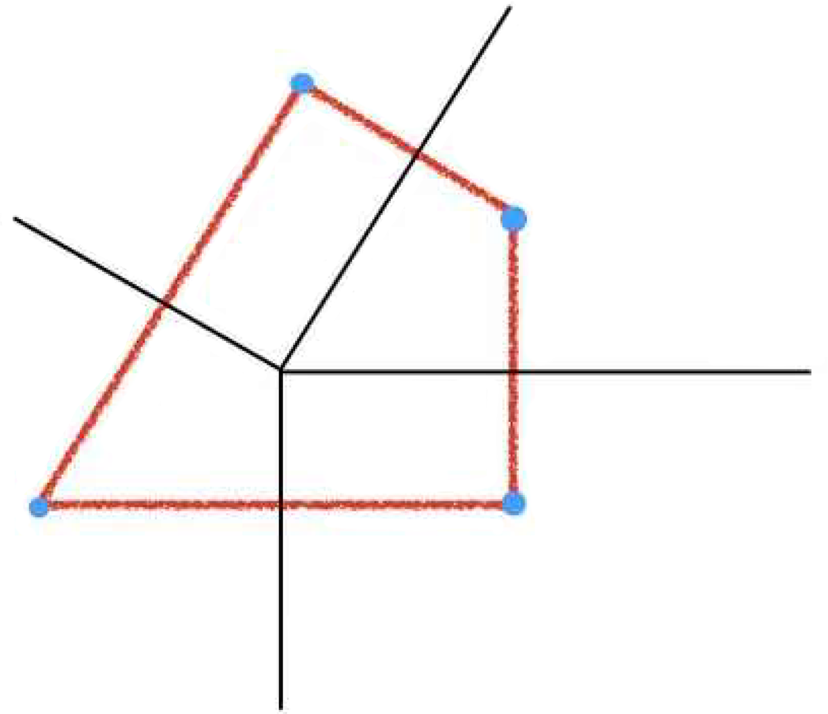
A virtual quadrangle with the same normal fan.
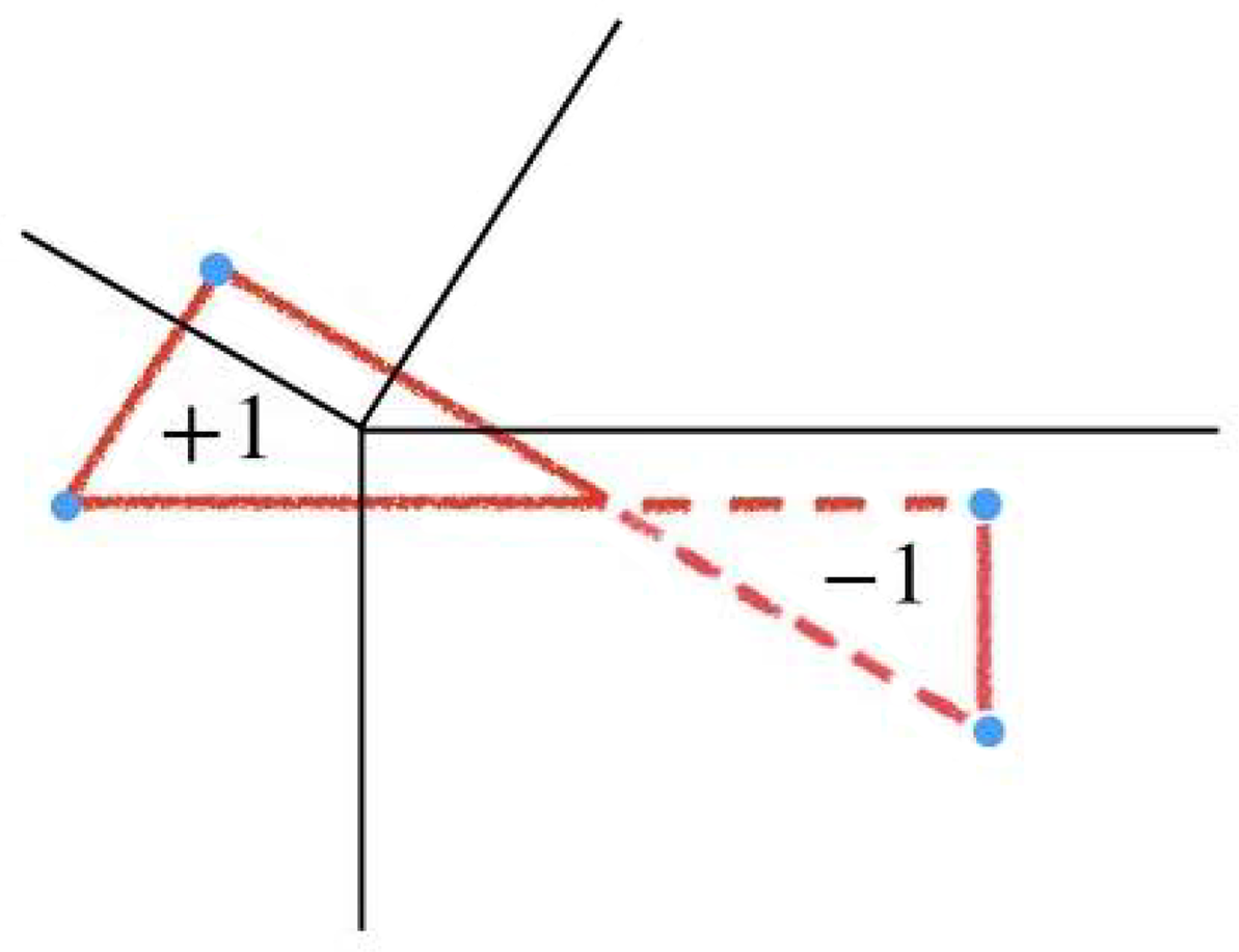
Remark 2.9 The notion of volume of a polytope extends to virtual polytopes via Theorem 2.1. For a virtual polytope $P \in {\mathcal V}(V^*)$
, we defined
$P \in {\mathcal V}(V^*)$
, we defined $\operatorname {vol}_n(P)$
to be the value of the volume polynomial at P. Similarly, the notion of the number of lattice points in a polytope extends to virtual polytopes as well. Let
$\operatorname {vol}_n(P)$
to be the value of the volume polynomial at P. Similarly, the notion of the number of lattice points in a polytope extends to virtual polytopes as well. Let $M \subset V^*$
be a full rank lattice. Let
$M \subset V^*$
be a full rank lattice. Let ${\mathcal V}(M)$
denote the collection of lattice virtual polytopes with respect to M, i.e., all virtual polytopes whose vertices are in M. In other words,
${\mathcal V}(M)$
denote the collection of lattice virtual polytopes with respect to M, i.e., all virtual polytopes whose vertices are in M. In other words, ${\mathcal V}(M)$
is the subgroup of
${\mathcal V}(M)$
is the subgroup of ${\mathcal V}(V^*)$
generated by lattice polytopes in
${\mathcal V}(V^*)$
generated by lattice polytopes in ${\mathcal P}(M)$
. By Theorem 2.2, there exists a (unique) polynomial F on
${\mathcal P}(M)$
. By Theorem 2.2, there exists a (unique) polynomial F on ${\mathcal V}(V^*)$
such that for any lattice polytope
${\mathcal V}(V^*)$
such that for any lattice polytope $P \in {\mathcal P}(V^*)$
, we have
$P \in {\mathcal P}(V^*)$
, we have $F(P) = |P \cap M|$
. For a virtual lattice polytope
$F(P) = |P \cap M|$
. For a virtual lattice polytope $P \in {\mathcal V}(M)$
, we define the number of lattice points in P to be
$P \in {\mathcal V}(M)$
, we define the number of lattice points in P to be $F(P)$
. The same applies to any valuation on the space of polytopes (see [Reference Khovanskii and PukhlikovKP93a]; see also Theorem 2.3 and the paragraph before it for the definition of a valuation).
$F(P)$
. The same applies to any valuation on the space of polytopes (see [Reference Khovanskii and PukhlikovKP93a]; see also Theorem 2.3 and the paragraph before it for the definition of a valuation).
Each polytope $P \in {\mathcal P}(V^*)$
is determined by its characteristic function
$P \in {\mathcal P}(V^*)$
is determined by its characteristic function ${\textbf 1}_P: V^* \to \{0, 1\}$
. We would like to extend the assignment
${\textbf 1}_P: V^* \to \{0, 1\}$
. We would like to extend the assignment $P \mapsto {\textbf 1}_P$
to virtual polytopes. The natural extension of the set of characteristic functions of convex polytopes (to a vector space) is the set of convex chains (defined by Khovanskii and Pukhlikov).
$P \mapsto {\textbf 1}_P$
to virtual polytopes. The natural extension of the set of characteristic functions of convex polytopes (to a vector space) is the set of convex chains (defined by Khovanskii and Pukhlikov).
Definition 2.2 (Convex chain)
A convex chain Z is a finite linear combination (with real coefficients) of characteristic functions of convex polytopes in $V^*$
, that is,
$V^*$
, that is, $Z = \sum _i \lambda _i {\textbf 1}_{\Delta _i}$
, where the
$Z = \sum _i \lambda _i {\textbf 1}_{\Delta _i}$
, where the $\Delta _i$
are convex polytopes in
$\Delta _i$
are convex polytopes in $V^*$
and
$V^*$
and $\lambda _i \in {\mathbb R}$
. We denote the set of convex chains by
$\lambda _i \in {\mathbb R}$
. We denote the set of convex chains by $\mathcal {Z}(V^*)$
. It is an infinite dimensional vector space with addition and scalar multiplication of functions.
$\mathcal {Z}(V^*)$
. It is an infinite dimensional vector space with addition and scalar multiplication of functions.
Moreover, in general, one can consider the characteristic functions of convex polyhedral cones.
Definition 2.3 (Conical convex chain)
A conical convex chain C is a finite linear combination (with real coefficients) of characteristic functions of shifted convex cones in $V^*$
, that is,
$V^*$
, that is, $C = \sum _i \lambda _i {\textbf 1}_{a_i + C_i}$
, where the
$C = \sum _i \lambda _i {\textbf 1}_{a_i + C_i}$
, where the $C_i$
are convex polyhedral cones in
$C_i$
are convex polyhedral cones in $V^*$
(with apex at the origin),
$V^*$
(with apex at the origin), $a_i \in V^*$
, and
$a_i \in V^*$
, and $\lambda _i \in {\mathbb R}$
. We denote the set of convex conical chains by
$\lambda _i \in {\mathbb R}$
. We denote the set of convex conical chains by $\mathcal {C}\mathcal {Z}(V^*)$
.
$\mathcal {C}\mathcal {Z}(V^*)$
.
A remarkable construction in [Reference Khovanskii and PukhlikovKP93a] is a “convolution” operation $*$
on
$*$
on $\mathcal {Z}(V^*)$
which makes it a commutative algebra (together with addition and scalar multiplication of functions). It has the property that for any two polytopes
$\mathcal {Z}(V^*)$
which makes it a commutative algebra (together with addition and scalar multiplication of functions). It has the property that for any two polytopes $P_1$
and
$P_1$
and $P_2$
, we have
$P_2$
, we have
 $$\begin{align*}{\textbf 1}_{P_1} * {\textbf 1}_{P_2} = {\textbf 1}_{P_1 + P_2}.\\[-15pt] \end{align*}$$
In particular, the identity element for the $*$
operation is
$*$
operation is ${\textbf 1}_{\{0\}}$
, the characteristic function of the origin.
${\textbf 1}_{\{0\}}$
, the characteristic function of the origin.
For a polytope P, it is shown in [Reference Khovanskii and PukhlikovKP93a] that the inverse (with respect to $*$
) of
$*$
) of ${\textbf 1}_P$
is the convex chain
${\textbf 1}_P$
is the convex chain $(-1)^{\dim P} {\textbf 1}_{P^\circ }$
, where
$(-1)^{\dim P} {\textbf 1}_{P^\circ }$
, where $P^\circ $
denotes the relative interior of P. In other words,
$P^\circ $
denotes the relative interior of P. In other words,
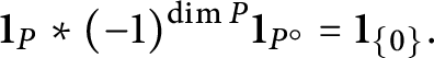 $$\begin{align*}{\textbf 1}_P * (-1)^{\dim P} {\textbf 1}_{P^\circ} = {\textbf 1}_{\{0\}}. \end{align*}$$
One verifies that
 $$\begin{align*}(-1)^{\dim P} {\textbf 1}_{P^\circ} = \sum_{Q \preceq P} (-1)^{\dim Q} {\textbf 1}_Q, \end{align*}$$
and hence $(-1)^{\dim P} {\textbf 1}_{P^\circ }$
is indeed a convex chain. It follows that
$(-1)^{\dim P} {\textbf 1}_{P^\circ }$
is indeed a convex chain. It follows that
 $$ \begin{align} \iota: P_1 - P_2 \mapsto {\textbf 1}_{P_1} * (-1)^{\dim P_2} {\textbf 1}_{P_2^\circ} = \sum_{Q \preceq P_2} (-1)^{\dim Q} {\textbf 1}_{P_1 + Q} \end{align} $$
defines a natural embedding of the group of virtual polytopes (with the Minkowski sum) into the semigroup of convex chains (with convolution $*$
). We refer to the right-hand side of (2.8) as the convex chain associated with the characteristic function of the virtual polytope
$*$
). We refer to the right-hand side of (2.8) as the convex chain associated with the characteristic function of the virtual polytope $P_1 - P_2$
. In fact, it is shown in [Reference Khovanskii and PukhlikovKP93a] that the image of
$P_1 - P_2$
. In fact, it is shown in [Reference Khovanskii and PukhlikovKP93a] that the image of $\iota $
coincides with the set of
$\iota $
coincides with the set of $*$
-invertible convex chains.
$*$
-invertible convex chains.
We can talk about vertices of a virtual polytope. For a virtual polytope $P \in {\mathcal V}(\Sigma )$
, the vertices are in one-to-one correspondence with the full dimensional cones in
$P \in {\mathcal V}(\Sigma )$
, the vertices are in one-to-one correspondence with the full dimensional cones in $\Sigma $
. Similarly, the notion of a tangent cone of a polytope extends to virtual polytopes. The tangent cones of
$\Sigma $
. Similarly, the notion of a tangent cone of a polytope extends to virtual polytopes. The tangent cones of $P \in {\mathcal V}(\Sigma )$
are in one-to-one correspondence with
$P \in {\mathcal V}(\Sigma )$
are in one-to-one correspondence with $\sigma \in \Sigma $
.
$\sigma \in \Sigma $
.
There is a generalization of the Brianchon–Gram theorem to convex chains (see [Reference Khovanskii and PukhlikovKP93a, Section 4, Proposition 2]). The Lawrence–Varchenko theorem also extends to simple virtual polytopes.
Theorem 2.10 (Lawrence–Varchenko for virtual polytopes)
Let P be a virtual polytope in $V^*$
, and let
$V^*$
, and let $\pi : V^* \to {\mathbb R}$
be the corresponding convex chain. Then
$\pi : V^* \to {\mathbb R}$
be the corresponding convex chain. Then
 $$ \begin{align} \pi = \sum_{v} (-1)^{n_v} {\textbf 1}_{T^\xi_{P, v}}, \end{align} $$
where the sum is over all the vertices v of P and $T^\xi _{P, v}$
and
$T^\xi _{P, v}$
and $n_v$
are as in Theorem 2.8.
$n_v$
are as in Theorem 2.8.
See Figure 12 for an illustration of (2.9).
Illustration of the Lawrence–Varchenko theorem for a virtual quadrangle.

2.7 Incidence algebra of a poset and Möbius inversion
For a nice reference about incidence algebra and Möbius inversion, see [Reference StanleySt12, Sections 3.6 and 3.7]. Let $\mathcal {P}$
be a finite poset with partial order
$\mathcal {P}$
be a finite poset with partial order $\prec $
. Let R be a commutative ring with
$\prec $
. Let R be a commutative ring with $1$
which we take as the ring of scalars. Let
$1$
which we take as the ring of scalars. Let $\tilde {\mathcal {P}} = \{(\tau , \sigma ) : \tau \preceq \sigma \} \subset \mathcal {P} \times \mathcal {P}$
be the collection of all intervals in
$\tilde {\mathcal {P}} = \{(\tau , \sigma ) : \tau \preceq \sigma \} \subset \mathcal {P} \times \mathcal {P}$
be the collection of all intervals in $\mathcal {P}$
. Let
$\mathcal {P}$
. Let $I(\mathcal {P}) = \{F: \tilde {\mathcal {P}} \to R \}$
be the set of functions from
$I(\mathcal {P}) = \{F: \tilde {\mathcal {P}} \to R \}$
be the set of functions from $\tilde {\mathcal {P}}$
to R. Clearly,
$\tilde {\mathcal {P}}$
to R. Clearly, $I = I(\mathcal {P})$
is an abelian group with addition of functions. One defines a convolution operation
$I = I(\mathcal {P})$
is an abelian group with addition of functions. One defines a convolution operation $*$
on I as follows. For
$*$
on I as follows. For $F, G \in I$
define
$F, G \in I$
define $F * G \in I$
by
$F * G \in I$
by
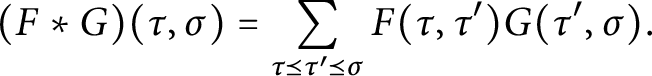 $$\begin{align*}(F * G)(\tau, \sigma) = \sum_{\tau \preceq \tau' \preceq \sigma} F(\tau, \tau') G(\tau', \sigma). \end{align*}$$
It can be verified that $(I, +, *)$
is an algebra over R, called incidence algebra of the poset
$(I, +, *)$
is an algebra over R, called incidence algebra of the poset $\mathcal {P}$
. In general,
$\mathcal {P}$
. In general, $I(\mathcal {P})$
is not commutative.
$I(\mathcal {P})$
is not commutative.
The identity (for the convolution operation $*$
) is the function
$*$
) is the function $\delta $
defined by
$\delta $
defined by
 $$\begin{align*}\delta(\tau, \sigma) = \begin{cases} 1, \quad \tau = \sigma, \\ 0, \quad \tau \neq \sigma. \end{cases} \end{align*}$$
A distinguished element of the incidence algebra is the constant function $\zeta (\tau , \sigma ) = 1$
, for any interval
$\zeta (\tau , \sigma ) = 1$
, for any interval $\tau \preceq \sigma $
. The Möbius inversion formula states that the function
$\tau \preceq \sigma $
. The Möbius inversion formula states that the function $\zeta $
is invertible and its inverse is the Möbius function
$\zeta $
is invertible and its inverse is the Möbius function $\mu $
. For the general poset
$\mu $
. For the general poset $\mathcal {P}$
, the Möbius function is constructed/defined inductively, but in specific examples, it can be defined/computed explicitly.
$\mathcal {P}$
, the Möbius function is constructed/defined inductively, but in specific examples, it can be defined/computed explicitly.
Example 2.11 (Poset of subsets of a finite set)
Let $\mathcal {P}$
be the poset of all subset of
$\mathcal {P}$
be the poset of all subset of $\{1, \ldots , d\}$
ordered by inclusion. It can be shown that the Möbius function in this case is given by
$\{1, \ldots , d\}$
ordered by inclusion. It can be shown that the Möbius function in this case is given by
 $$\begin{align*}\mu(I, J) = (-1)^{|I| - |J|}, \quad J \subset I, \end{align*}$$
and the Möbius inversion formula recovers the inclusion–exclusion principle.
The following is the main example of a poset that we will be concerned with in the paper.
Example 2.12 (Poset of faces of a convex polyhedral cone)
Let $\mathcal {P}$
be the poset of all faces of a given convex polyhedral cone
$\mathcal {P}$
be the poset of all faces of a given convex polyhedral cone $C \subset {\mathbb R}^n$
. If
$C \subset {\mathbb R}^n$
. If $\sigma $
is simplicial of dimension d, then this poset is the same as the poset of all subsets of
$\sigma $
is simplicial of dimension d, then this poset is the same as the poset of all subsets of $\{1, \ldots , d\}$
above. It can be shown that the Möbius function in this case is given by
$\{1, \ldots , d\}$
above. It can be shown that the Möbius function in this case is given by
 $$ \begin{align*}\mu(\tau, \sigma) = (-1)^{\dim \sigma - \dim \tau}, \quad \tau \preceq \sigma.\end{align*} $$
3 Convergence
In this section, we give some combinatorial/geometric results that contain the combinatorial ingredients of Arthur’s result on the convergence and polynomiality (in a truncation parameter T) of the truncated trace $J^T(f)$
in his noninvariant trace formula. See [Reference ArthurAr78, Section 7] and [Reference ArthurAr81, Section 2] as well as the survey [Reference ArthurAr05, Sections 8 and 9].
$J^T(f)$
in his noninvariant trace formula. See [Reference ArthurAr78, Section 7] and [Reference ArthurAr81, Section 2] as well as the survey [Reference ArthurAr05, Sections 8 and 9].
We continue to denote the n-dimensional real vector space we fixed in Section 2 by V. We choose an inner product $\langle \cdot , \cdot \rangle $
on V and use it to identify V with its dual. Our results in this section depend on the choice of this inner product. In particular, we view the dual cone
$\langle \cdot , \cdot \rangle $
on V and use it to identify V with its dual. Our results in this section depend on the choice of this inner product. In particular, we view the dual cone $\sigma ^\vee $
as a subset of V itself,
$\sigma ^\vee $
as a subset of V itself,
 $$\begin{align*}\sigma^\vee := \left\{ x \in V : \langle x , y \rangle \geqslant 0, \text{for all } y \in \sigma\right\}. \end{align*}$$
Our starting point is a full dimensional, complete, simplicial fan $\Sigma $
in V. Let
$\Sigma $
in V. Let $\Delta \in \mathcal {P}(\Sigma )$
be a convex polytope whose normal fan is
$\Delta \in \mathcal {P}(\Sigma )$
be a convex polytope whose normal fan is $\Sigma $
. Suppose that we are given a collection of continuous functions
$\Sigma $
. Suppose that we are given a collection of continuous functions
 $$ \begin{align} K_\sigma: V \longrightarrow {\mathbb C}, \quad \sigma \in \Sigma. \end{align} $$
To these data, we associate the truncated function $k_\Delta : V \longrightarrow {\mathbb C}$
defined by
$k_\Delta : V \longrightarrow {\mathbb C}$
defined by
 $$ \begin{align} k_\Delta(x) = \sum_{\sigma \in \Sigma} (-1)^{\dim\sigma}~K_\sigma(x) ~{\textbf 1}_{T^-_{\Delta, \sigma}}(x), \end{align} $$
where $T^-_{\Delta , \sigma } = T^-_{\Delta , Q_\sigma }$
is the outward tangent cone, as in (2.3), of the face
$T^-_{\Delta , \sigma } = T^-_{\Delta , Q_\sigma }$
is the outward tangent cone, as in (2.3), of the face $Q_\sigma $
of
$Q_\sigma $
of $\Delta $
that stands in bijection with
$\Delta $
that stands in bijection with $\sigma $
as in (2.4). The main result of this section is to prove that if the functions
$\sigma $
as in (2.4). The main result of this section is to prove that if the functions $K_\sigma $
satisfy certain assumptions, then the integral of
$K_\sigma $
satisfy certain assumptions, then the integral of $k_\Delta $
over V is absolutely convergent. In particular, these assumptions hold when the functions
$k_\Delta $
over V is absolutely convergent. In particular, these assumptions hold when the functions $K_\sigma $
satisfy certain growth conditions as we explain below. The latter is the setting in which ATF appears.
$K_\sigma $
satisfy certain growth conditions as we explain below. The latter is the setting in which ATF appears.
For a cone $\sigma \in \Sigma $
, let
$\sigma \in \Sigma $
, let $W(\sigma ) = \left \{w_i \in V : i \in I\right \}$
be a set of unit edge vectors of
$W(\sigma ) = \left \{w_i \in V : i \in I\right \}$
be a set of unit edge vectors of $\sigma $
. We also let
$\sigma $
. We also let $B(\sigma ) = \left \{b_i \in V : i \in I\right \}$
denote the set of unit, inward, facet normals in
$B(\sigma ) = \left \{b_i \in V : i \in I\right \}$
denote the set of unit, inward, facet normals in $\operatorname {Span}(\sigma )$
to the facets of
$\operatorname {Span}(\sigma )$
to the facets of $\sigma $
. Note that the
$\sigma $
. Note that the $b_i$
form a basis of
$b_i$
form a basis of $\operatorname {Span}(\sigma )$
dual to the
$\operatorname {Span}(\sigma )$
dual to the $w_i$
, i.e.,
$w_i$
, i.e.,
 $$\begin{align*}\langle w_i, b_j \rangle = \delta_{i,j}, \quad i,j \in I. \end{align*}$$
When $\sigma $
is full dimensional,
$\sigma $
is full dimensional, $B(\sigma )$
is the set of edge vectors of the dual cone
$B(\sigma )$
is the set of edge vectors of the dual cone $\sigma ^\vee $
.
$\sigma ^\vee $
.
Definition 3.1 (Acute cone and acute fan)
We say that a convex cone $\sigma $
in V is acute if
$\sigma $
in V is acute if $ \sigma \subseteq \sigma ^\vee $
. We call the fan
$ \sigma \subseteq \sigma ^\vee $
. We call the fan $\Sigma $
acute if all its cones are acute.
$\Sigma $
acute if all its cones are acute.
Notice that our definition of acute allows for right angles. We also remark that the notion of acute depends on the inner product we have chosen in V. Indeed, the acute assumption will be crucial for the convergence results below to hold as Example 3.6 shows.
Observe that
 $$ \begin{align} \sigma \mbox{ is acute} \quad \Longleftrightarrow \quad \langle w_i, w_j \rangle \geqslant 0, \quad i,j \in I. \end{align} $$
It follows from Definition 3.1 that if $\sigma $
is acute, then for
$\sigma $
is acute, then for $x \in \operatorname {Span}(\sigma )$
,
$x \in \operatorname {Span}(\sigma )$
,
 $$ \begin{align} \langle x , b_i \rangle> 0 \mbox{ for all } i \in I \quad \Longrightarrow \quad \langle x , w_i \rangle > 0 \mbox{ for all } i \in I. \end{align} $$
Next, fix a pair of cones $\sigma _2 \preceq \sigma _1$
in
$\sigma _2 \preceq \sigma _1$
in $\Sigma $
. Write
$\Sigma $
. Write $W(\sigma _1) = \left \{w_i \in V : i \in I_1\right \}$
and
$W(\sigma _1) = \left \{w_i \in V : i \in I_1\right \}$
and $B(\sigma _1) = \left \{b_i \in V : i \in I_1\right \}$
as above. Then
$B(\sigma _1) = \left \{b_i \in V : i \in I_1\right \}$
as above. Then $W(\sigma _2) = \left \{w_i : i \in I_2 \right \}$
for some
$W(\sigma _2) = \left \{w_i : i \in I_2 \right \}$
for some $I_2 \subseteq I_1$
and the set
$I_2 \subseteq I_1$
and the set $\left \{b_j : j \in I_1 \setminus I_2 \right \}$
consists of vectors normal to
$\left \{b_j : j \in I_1 \setminus I_2 \right \}$
consists of vectors normal to $\sigma _2$
. (However,
$\sigma _2$
. (However, $B(\sigma _2)$
is not
$B(\sigma _2)$
is not $\left \{b_j : j \in I_2 \right \}$
as the latter depends on
$\left \{b_j : j \in I_2 \right \}$
as the latter depends on $\sigma _1$
.)
$\sigma _1$
.)
Define
 $$ \begin{align} C_{\sigma_1} = C_{\sigma_1}^0 := \left\{x \in \operatorname{Span}(\sigma_1) : \langle x, b_j \rangle> 0, \mbox{ for all } j \in I_1 \right\}, \end{align} $$
and similarly, define
 $$ \begin{align} {\widehat{C}}_{\sigma_1} = \widehat{C}_{\sigma_1}^0 := \left\{x \in \operatorname{Span}(\sigma_1) : \langle x, w_i\rangle> 0, \mbox{ for all } i \in I_1 \right\}. \end{align} $$
More generally, we define
 $$ \begin{align} C_{\sigma_1}^{\sigma_2} := \left\{x \in \operatorname{Span}(\sigma_1) : \langle x, b_j \rangle> 0, \mbox{ for all } j \in I_1 \setminus I_2 \right\}, \end{align} $$
and
 $$ \begin{align} \widehat{C}_{\sigma_1}^{\sigma_2} := \left\{x \in \operatorname{Span}(\sigma_1) : \langle x, w_i\rangle> 0, \mbox{ for all } i \in I_1 \setminus I_2 \right\}. \end{align} $$
Next, we define the following subsets of V which play a crucial role in our results.
Definition 3.2 Let $\Sigma $
be a full dimensional, complete, simplicial, acute fan in V. Assume that
$\Sigma $
be a full dimensional, complete, simplicial, acute fan in V. Assume that $\sigma _2 \preceq \sigma _1$
are two cones in
$\sigma _2 \preceq \sigma _1$
are two cones in $\Sigma $
with unit edge vectors indexed by
$\Sigma $
with unit edge vectors indexed by $I_2 \subset I_1$
as above.
$I_2 \subset I_1$
as above.
-
(a) Define
$S_{\sigma _1}^{\sigma _2}$
to be the set of
$x \in \operatorname {Span}(\sigma _1) \cap \sigma _1^\vee $
such that the face of
$\sigma _1$
that is nearest to x is the cone generated by
$\left \{w_i : i \in I_1 \setminus I_2 \right \}$
. Also, let
${\textbf 1}_{S_{\sigma _1}^{\sigma _2}}$
denote its characteristic function. (See Section 2.4.) -
(b) Define the “shifted” subset
(3.9)
$$ \begin{align} R_{\sigma_1}^{\sigma_2} := Q_{\sigma_1} + S_{\sigma_1}^{\sigma_2} = \left\{x_0 + x \in V : x_0 \in Q_{\sigma_1} \mbox { and } x \in S_{\sigma_1}^{\sigma_2} \right\}. \end{align} $$


We also note that while the subsets $S_{\sigma _1}^{\sigma _2}$
may have smaller dimensions, the subsets
$S_{\sigma _1}^{\sigma _2}$
may have smaller dimensions, the subsets $R_{\sigma _1}^{\sigma _2}$
, when nonempty, are always full dimensional because the dimension of
$R_{\sigma _1}^{\sigma _2}$
, when nonempty, are always full dimensional because the dimension of $Q_{\sigma _1}$
(as an affine space) and that of
$Q_{\sigma _1}$
(as an affine space) and that of $S_{\sigma _1}^{\sigma _2}$
add up to
$S_{\sigma _1}^{\sigma _2}$
add up to $n = \dim V$
.
$n = \dim V$
.
As Lemma 3.1 below shows, the $S_{\sigma _1}^{\sigma _2}$
are the analogues of the subsets appearing in [Reference ArthurAr78, Lemma 6.1], which also appear to play a similar crucial role in Arthur’s results on convergence and polynomiality.
$S_{\sigma _1}^{\sigma _2}$
are the analogues of the subsets appearing in [Reference ArthurAr78, Lemma 6.1], which also appear to play a similar crucial role in Arthur’s results on convergence and polynomiality.
Lemma 3.1 With $\sigma _2 \preceq \sigma _1$
in
$\sigma _2 \preceq \sigma _1$
in $\Sigma $
, the vectors
$\Sigma $
, the vectors $w_i$
and
$w_i$
and $b_i$
, and
$b_i$
, and $I_2 \subset I_1$
as above, we have
$I_2 \subset I_1$
as above, we have
 $$ \begin{align} S_{\sigma_1}^{\sigma_2} = \left\{x \in \operatorname{Span}(\sigma_1) : \begin{array}{ll} \langle x, b_j \rangle> 0, & j \in I_1 \setminus I_2 \\ \langle x, b_j \rangle \leqslant 0, & j \in I_2 \\ \langle x, w_i \rangle > 0, & i \in I_1 \\ \end{array} \right\}. \end{align} $$
Proof Write $\tau = \operatorname {Cone}\left (w_i : i \in I_1 \setminus I_2 \right )$
. Fix
$\tau = \operatorname {Cone}\left (w_i : i \in I_1 \setminus I_2 \right )$
. Fix $x \in \operatorname {Span}(\sigma _1) \cap \sigma ^\vee _1$
. Now, x belongs to
$x \in \operatorname {Span}(\sigma _1) \cap \sigma ^\vee _1$
. Now, x belongs to $S_{\sigma _1}^{\sigma _2}$
if and only if among all the faces of
$S_{\sigma _1}^{\sigma _2}$
if and only if among all the faces of $\sigma _1$
the face
$\sigma _1$
the face $\tau $
is the unique face that is nearest to x. Note that the distances to the faces of
$\tau $
is the unique face that is nearest to x. Note that the distances to the faces of $\sigma _1$
are controlled by the normal vectors
$\sigma _1$
are controlled by the normal vectors $b_j$
and for
$b_j$
and for $\tau $
to be the unique nearest face, we must have
$\tau $
to be the unique nearest face, we must have $\langle x, b_j \rangle> 0$
for
$\langle x, b_j \rangle> 0$
for $j \in I_1 \setminus I_2$
while
$j \in I_1 \setminus I_2$
while $\langle x, b_j \rangle \leqslant 0$
for
$\langle x, b_j \rangle \leqslant 0$
for $j \in I_2$
. This implies that
$j \in I_2$
. This implies that $x \in S_{\sigma _1}^{\sigma _2}$
satisfies the first two sets of inequalities on the right-hand side of (3.10). Also, x satisfies the third set of inequalities on the right-hand side of (3.10) by (3.4) because
$x \in S_{\sigma _1}^{\sigma _2}$
satisfies the first two sets of inequalities on the right-hand side of (3.10). Also, x satisfies the third set of inequalities on the right-hand side of (3.10) by (3.4) because $x \in \sigma ^\vee _1$
, a cone whose edge vectors are the
$x \in \sigma ^\vee _1$
, a cone whose edge vectors are the $b_i$
’s.
$b_i$
’s.
Next, assume that x belongs to the right-hand side of (3.10). The first two sets of inequalities imply that $\sigma _2$
is the unique nearest face of
$\sigma _2$
is the unique nearest face of $\sigma _1$
to x and the third set of inequalities means that
$\sigma _1$
to x and the third set of inequalities means that $x \in \sigma _1^\vee $
.▪
$x \in \sigma _1^\vee $
.▪
Remark 3.2 Even though we start with simplicial cones $\sigma _2 \preceq \sigma _1$
, the cone
$\sigma _2 \preceq \sigma _1$
, the cone $S_{\sigma _1}^{\sigma _2}$
may not be simplicial. As an example, consider
$S_{\sigma _1}^{\sigma _2}$
may not be simplicial. As an example, consider $V = {\mathbb R}^3$
, and let
$V = {\mathbb R}^3$
, and let $w_1 = e_1, w_2 = e_2$
, and
$w_1 = e_1, w_2 = e_2$
, and $w_3=e_1+e_2+e_3$
. Take
$w_3=e_1+e_2+e_3$
. Take $\sigma _2 = \operatorname {Cone}(w_3) \preceq \sigma _1 = \operatorname {Cone}(w_1, w_2, w_3)$
. We then have
$\sigma _2 = \operatorname {Cone}(w_3) \preceq \sigma _1 = \operatorname {Cone}(w_1, w_2, w_3)$
. We then have $b_1 = e_1 - e_3, b_2 = e_2 - e_3$
, and
$b_1 = e_1 - e_3, b_2 = e_2 - e_3$
, and $b_3=e_3$
. A simple calculation then shows that
$b_3=e_3$
. A simple calculation then shows that $S_{\sigma _1}^{\sigma _2} = \operatorname {Cone}(w_1,w_2,b_1,b_2)$
, which is not simplicial.
$S_{\sigma _1}^{\sigma _2} = \operatorname {Cone}(w_1,w_2,b_1,b_2)$
, which is not simplicial.
The following is a type of double nearest face partition that will help us prove our convergence results.
Lemma 3.3 Let $\Sigma $
be a full dimensional, complete, simplicial fan in V which is assumed to be acute. Let
$\Sigma $
be a full dimensional, complete, simplicial fan in V which is assumed to be acute. Let $\Delta \in \mathcal {P}(\Sigma )$
be a convex polytope whose normal fan is
$\Delta \in \mathcal {P}(\Sigma )$
be a convex polytope whose normal fan is $\Sigma $
. Then, for any
$\Sigma $
. Then, for any $\sigma \in \Sigma $
, the outward tangent cone
$\sigma \in \Sigma $
, the outward tangent cone $T^-_{\Delta , \sigma }$
has the partition
$T^-_{\Delta , \sigma }$
has the partition
 $$ \begin{align} T^-_{\Delta, \sigma} = \bigsqcup\limits_{\left\{\sigma_1\in\Sigma \, : \, \sigma\preceq\sigma_1\right\}}~ \bigsqcup\limits_{\left\{\sigma_2 \in \Sigma : \sigma_2\preceq\sigma\right\}} R_{\sigma_1}^{\sigma_2}. \end{align} $$
Proof Consider the inner disjoint union in (3.11) first. Fix $\sigma _1$
in
$\sigma _1$
in $\Sigma $
with
$\Sigma $
with $\sigma \preceq \sigma _1$
. Write
$\sigma \preceq \sigma _1$
. Write $W(\sigma _1) = \left \{w_i \in V : i \in I_1 \right \}$
, and assume that
$W(\sigma _1) = \left \{w_i \in V : i \in I_1 \right \}$
, and assume that $I_2 \subseteq I \subseteq I_1$
are such that
$I_2 \subseteq I \subseteq I_1$
are such that $W(\sigma ) = \left \{w_i \in V : i \in I \right \}$
and similarly for
$W(\sigma ) = \left \{w_i \in V : i \in I \right \}$
and similarly for $W(\sigma _2)$
. Also, write
$W(\sigma _2)$
. Also, write $B(\sigma _1) = \left \{b_j \in V : j \in I_1 \right \}$
. Notice that
$B(\sigma _1) = \left \{b_j \in V : j \in I_1 \right \}$
. Notice that $b_j$
is normal to
$b_j$
is normal to $\sigma $
for
$\sigma $
for $j \in I_1 \setminus I$
and
$j \in I_1 \setminus I$
and $b_j$
is normal to
$b_j$
is normal to $\sigma _2$
for
$\sigma _2$
for $j \in I_1 \setminus I_2$
.
$j \in I_1 \setminus I_2$
.
Simply considering all the subsets of I, we see that
 $$\begin{align*}A_{\sigma_1}^\sigma := \bigsqcup\limits_{\sigma_2 : \sigma_2\preceq\sigma \preceq \sigma_1} R_{\sigma_1}^{\sigma_2} = \left\{ x \in V : \begin{array}{ll} \langle x-q , b_i \rangle> 0, & i \in I_1 \setminus I, \\ \langle x-q , w_i \rangle > 0, & i \in I_1, \\ \end{array} \mbox{ for some } q \in Q_{\sigma_1} \right\}. \end{align*}$$
This is because, for $q \in Q_{\sigma _1}$
, the set
$q \in Q_{\sigma _1}$
, the set $q+ S_{\sigma _1}^{\sigma _2}$
is, by (3.10), given by
$q+ S_{\sigma _1}^{\sigma _2}$
is, by (3.10), given by
 $$\begin{align*}\begin{array}{ll} \langle x-q , b_i \rangle> 0, & i \in I_1 \setminus I_2 = (I_1 \setminus I) \sqcup (I \setminus I_2), \\ \langle x-q , b_i \rangle \leqslant0, & i \in I_2, \\ \langle x-q , w_i \rangle > 0, & i \in I_1. \\ \end{array} \end{align*}$$
In the disjoint union over all subsets $I_2$
of I corresponding to the faces
$I_2$
of I corresponding to the faces $\sigma _2$
of
$\sigma _2$
of $\sigma $
, the first set of inequalities for
$\sigma $
, the first set of inequalities for $i \in I_1 \setminus I$
are common for all the subsets
$i \in I_1 \setminus I$
are common for all the subsets $I_2$
and the remaining inequalities along with the second set of inequalities cover all possible signs for
$I_2$
and the remaining inequalities along with the second set of inequalities cover all possible signs for $\langle x-q , b_i \rangle $
for all
$\langle x-q , b_i \rangle $
for all $i \in I$
. Moreover, we have
$i \in I$
. Moreover, we have $\langle x-q , w_i \rangle> 0$
for
$\langle x-q , w_i \rangle> 0$
for $i \in I_1$
. This proves our claim about the inner union and, in fact, already proves the lemma for the case when
$i \in I_1$
. This proves our claim about the inner union and, in fact, already proves the lemma for the case when $\sigma $
is full dimensional since we only have the inner union in that case.
$\sigma $
is full dimensional since we only have the inner union in that case.
Next, we consider the outer union. The assertion of the lemma now amounts to a nearest face partition. The set $T^-_{\Delta , \sigma }$
consists of
$T^-_{\Delta , \sigma }$
consists of $x \in V$
satisfying
$x \in V$
satisfying $\langle x-q , w_i \rangle> 0, i \in I$
for every
$\langle x-q , w_i \rangle> 0, i \in I$
for every $q \in Q_\sigma $
. Fix one such x. There is a unique face
$q \in Q_\sigma $
. Fix one such x. There is a unique face $Q_{\sigma _1}$
of
$Q_{\sigma _1}$
of $\Delta $
with
$\Delta $
with $\sigma \preceq \sigma _1$
such that the distance from x to
$\sigma \preceq \sigma _1$
such that the distance from x to $Q_{\sigma _1}$
is smallest among all the faces contained in
$Q_{\sigma _1}$
is smallest among all the faces contained in $Q_\sigma $
. Note that the distances are controlled by the normal vectors
$Q_\sigma $
. Note that the distances are controlled by the normal vectors $b_j$
and for the smallest distance to occur for the face
$b_j$
and for the smallest distance to occur for the face $Q_{\sigma _1}$
of
$Q_{\sigma _1}$
of $Q_\sigma $
, we must have
$Q_\sigma $
, we must have $\langle x-q , b_j \rangle> 0$
for
$\langle x-q , b_j \rangle> 0$
for $j \in I_1 \setminus I$
and
$j \in I_1 \setminus I$
and $\langle x-q , b_j \rangle \leqslant 0$
for
$\langle x-q , b_j \rangle \leqslant 0$
for $j \in I_0 \setminus I_1$
for any
$j \in I_0 \setminus I_1$
for any $I_0 \supset I$
with
$I_0 \supset I$
with $\sigma _0 \in \Sigma $
for some
$\sigma _0 \in \Sigma $
for some $q \in Q_{\sigma _1}$
. Therefore, among the
$q \in Q_{\sigma _1}$
. Therefore, among the $A_{\sigma _1'}^\sigma $
with
$A_{\sigma _1'}^\sigma $
with $\sigma \preceq \sigma _1'$
, only
$\sigma \preceq \sigma _1'$
, only $A_{\sigma _1}^\sigma $
contains x. Hence, (3.11) holds.▪
$A_{\sigma _1}^\sigma $
contains x. Hence, (3.11) holds.▪
Let us also fix the following notation. For $\sigma _2 \preceq \sigma _1$
in
$\sigma _2 \preceq \sigma _1$
in $\Sigma $
, define the functions
$\Sigma $
, define the functions
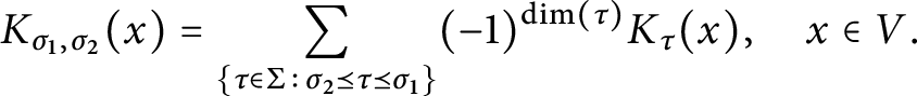 $$ \begin{align} K_{\sigma_1, \sigma_2}(x) = \sum_{\left\{\tau\in\Sigma \, : \, \sigma_2 \preceq \tau \preceq \sigma_1 \right\}} (-1)^{\dim(\tau)} K_\tau(x), \quad x \in V. \end{align} $$
We are now prepared to state our first convergence result.
Theorem 3.4 (Absolute convergence)
Let $\Sigma $
be a full dimensional, complete, simplicial fan in V which is assumed to be acute. Let
$\Sigma $
be a full dimensional, complete, simplicial fan in V which is assumed to be acute. Let $\Delta \in \mathcal {P}(\Sigma )$
be a simple full dimensional polytope in V whose normal fan is
$\Delta \in \mathcal {P}(\Sigma )$
be a simple full dimensional polytope in V whose normal fan is $\Sigma $
. Suppose that a collection of functions
$\Sigma $
. Suppose that a collection of functions $(K_\sigma )_{\sigma \in \Sigma }$
is given as in (
3.1
) and
$(K_\sigma )_{\sigma \in \Sigma }$
is given as in (
3.1
) and $k_\Delta $
is defined as in (
3.2
).
$k_\Delta $
is defined as in (
3.2
).
For each pair $\sigma _2 \preceq \sigma _1$
in
$\sigma _2 \preceq \sigma _1$
in $\Sigma $
, assume that the function
$\Sigma $
, assume that the function $K_{\sigma _1,\sigma _2}$
is absolutely integrable on the set
$K_{\sigma _1,\sigma _2}$
is absolutely integrable on the set $R_{\sigma _1}^{\sigma _2}$
. Then
$R_{\sigma _1}^{\sigma _2}$
. Then
 $$ \begin{align} J_{\Sigma}(\Delta) := \int\limits_V k_\Delta(x) \, dx\\[-15pt]\nonumber \end{align} $$
is absolutely convergent. Recall that $R_{\sigma _1}^{\sigma _2}$
is defined by (
3.9
) and
$R_{\sigma _1}^{\sigma _2}$
is defined by (
3.9
) and $K_{\sigma _1,\sigma _2}$
by (
3.12
).
$K_{\sigma _1,\sigma _2}$
by (
3.12
).
Proof Recall that $k_\Delta (x)$
is defined in terms of outward tangent cones
$k_\Delta (x)$
is defined in terms of outward tangent cones $T^-_{\Delta , \sigma }$
. It follows from Lemma 3.3 that
$T^-_{\Delta , \sigma }$
. It follows from Lemma 3.3 that
 $$ \begin{align*} k_\Delta(x) & = \sum_{\sigma \in \Sigma} (-1)^{\dim(\sigma)} K_\sigma(x) ~{\textbf 1}_{T^-_{\Delta, \sigma}}(x) \\ & = \sum\limits_{\sigma \in \Sigma} (-1)^{\dim(\sigma)} K_\sigma(x) \left( \sum\limits_{\sigma_1 : \sigma \preceq \sigma_1} \sum\limits_{\sigma_2 : \sigma_2 \preceq \sigma} {\textbf 1}_{R_{\sigma_1}^{\sigma_2}}(x) \right) \\ & = \sum\limits_{\sigma_2 \preceq \sigma_1} K_{\sigma_1,\sigma_2}(x) {\textbf 1}_{R_{\sigma_1}^{\sigma_2}}(x).\\[-15pt] \end{align*} $$
Hence,
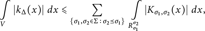 $$\begin{align*}\int\limits_V \left| k_\Delta(x) \right| \, dx \leqslant \sum\limits_{\left\{\sigma_1,\sigma_2\in\Sigma \, : \, \sigma_2 \preceq \sigma_1\right\}}~ \int\limits_{R_{\sigma_1}^{\sigma_2}} \left| K_{\sigma_1,\sigma_2}(x) \right| \, dx,\\[-15pt] \end{align*}$$
and each of the integrals on the right-hand side is finite by assumption. Therefore, the integral on the left-hand side is finite.▪
A special case of Theorem 3.4 is particularly suitable for applications to Arthur’s non-invariant trace formula. To state it, we review the following standard notions of growth.
Let $\sigma $
be a cone in V. A function
$\sigma $
be a cone in V. A function $K: V \to {\mathbb C}$
is said to be of order N in
$K: V \to {\mathbb C}$
is said to be of order N in $\sigma $
if there is a constant
$\sigma $
if there is a constant $C = C_{K,N}$
such that
$C = C_{K,N}$
such that
 $$\begin{align*}|K(x)| \leq C \, |x|^N\\[-15pt] \end{align*}$$
for x in $\sigma $
with
$\sigma $
with $|x|$
sufficiently large. In other words,
$|x|$
sufficiently large. In other words, $K(x) = O(|x|^{N})$
as x tends to
$K(x) = O(|x|^{N})$
as x tends to $\infty $
in
$\infty $
in $\sigma $
. We say K is rapidly decreasing on
$\sigma $
. We say K is rapidly decreasing on $\sigma $
if, for every
$\sigma $
if, for every $N>0$
, we have
$N>0$
, we have $K(x) = O(|x|^{-N})$
as x tends to
$K(x) = O(|x|^{-N})$
as x tends to $\infty $
in
$\infty $
in $\sigma $
.
$\sigma $
.
Theorem 3.5 Let $\Sigma $
be a full dimensional, complete, simplicial fan in V which is assumed to be acute, and let
$\Sigma $
be a full dimensional, complete, simplicial fan in V which is assumed to be acute, and let $(K_\sigma )_{\sigma \in \Sigma }$
be a collection of continuous functions as in (
3.1
). Assume that the following two assumptions are satisfied:
$(K_\sigma )_{\sigma \in \Sigma }$
be a collection of continuous functions as in (
3.1
). Assume that the following two assumptions are satisfied:
-
(i) For all
$\sigma \in \Sigma $
, the function
$K_\sigma $
is constant in the direction of
$\operatorname {Span}(\sigma )$
(i.e., a function on
$\sigma ^\perp $
). -
(ii) For all pairs of cones
$\sigma _2 \preceq \sigma _1$
in
$\Sigma $
with the subset
$S_{\sigma _1}^{\sigma _2}$
nonempty, the function
$K_{\sigma _1,\sigma _2}$
is of order
$N = -(n_1+\epsilon )$
for some
$\epsilon> 0$
in every shifted neighborhood
$B(y,\delta ) + S_{\sigma _1}^{\sigma _2}$
for all
$y \in V$
where
$B(y,\delta )$
is a (small) ball in V of positive radius
$\delta $
around y, and
$n_1 = \dim \sigma _1$
. In particular, this condition is satisfied if
$K_{\sigma _1,\sigma _2}$
is rapidly decreasing on the shifted neighborhoods.


Then, for $\Delta \in \mathcal P(\Sigma )$
, the integral (
3.13
) defining
$\Delta \in \mathcal P(\Sigma )$
, the integral (
3.13
) defining $J_{\Sigma }(\Delta )$
converges absolutely.
$J_{\Sigma }(\Delta )$
converges absolutely.
Proof By Theorem 3.4, it is enough to prove that the two assumptions in the statement imply that
 $$\begin{align*}\int\limits_{R_{\sigma_1}^{\sigma_2}} \left| K_{\sigma_1,\sigma_2}(x) \right| dx < \infty \end{align*}$$
for all pairs $\sigma _2 \preceq \sigma _1$
in
$\sigma _2 \preceq \sigma _1$
in $\Sigma $
.
$\Sigma $
.
We may replace the domain of integration by its closure. Also, recall that the closure of $R_{\sigma _1}^{\sigma _2}$
is equal to closure of
$R_{\sigma _1}^{\sigma _2}$
is equal to closure of $Q_{\sigma _1}$
, which is compact, plus the closure of
$Q_{\sigma _1}$
, which is compact, plus the closure of $S_{\sigma _1}^{\sigma _2}$
, which can be given by making all the inequalities in (3.10) nonstrict. Note that
$S_{\sigma _1}^{\sigma _2}$
, which can be given by making all the inequalities in (3.10) nonstrict. Note that $S_{\sigma _1}^{\sigma _2}$
is a cone, even though it may be nonsimplicial.
$S_{\sigma _1}^{\sigma _2}$
is a cone, even though it may be nonsimplicial.
To estimate the integral above, we apply Fubini’s theorem to break the integral as three iterated integrals: an integral over $Q_{\sigma _1}$
, an integral over
$Q_{\sigma _1}$
, an integral over $A = \sigma _2^\perp \cap \operatorname {Span}(\sigma _1)$
, and a third integral in the direction of
$A = \sigma _2^\perp \cap \operatorname {Span}(\sigma _1)$
, and a third integral in the direction of $\sigma _2$
.
$\sigma _2$
.
Note that $\operatorname {Span}(\sigma _2)$
does not intersect
$\operatorname {Span}(\sigma _2)$
does not intersect $S_{\sigma _1}^{\sigma _2}$
because, for any
$S_{\sigma _1}^{\sigma _2}$
because, for any $x \in \operatorname {Span}(\sigma _2)$
, the third set of inequalities in (3.1) for
$x \in \operatorname {Span}(\sigma _2)$
, the third set of inequalities in (3.1) for $i \in I_2$
and (3.4) imply that x cannot satisfy the second set of inequalities in (3.1). This observation and our first assumption imply that the contribution of the integral over
$i \in I_2$
and (3.4) imply that x cannot satisfy the second set of inequalities in (3.1). This observation and our first assumption imply that the contribution of the integral over $\sigma _2$
is bounded, up to a constant, by the product of the integrand with
$\sigma _2$
is bounded, up to a constant, by the product of the integrand with $|x|^{n_2},$
where
$|x|^{n_2},$
where $n_2 = \dim \sigma _2$
. Hence, the integral above is bounded, up to a constant, by
$n_2 = \dim \sigma _2$
. Hence, the integral above is bounded, up to a constant, by
 $$\begin{align*}\int\limits_{Q_{\sigma_1}} \int\limits_{A} \left| K_{\sigma_1,\sigma_2}(x) \right| |x|^{n_2} dx. \end{align*}$$
Next, using the second assumption and the fact that $Q_{\sigma _1}$
is compact, we may cover the domain of integration by a finite number of shifted neighborhoods. Therefore, up to a constant, the integral over A, which is a cone of dimension
$Q_{\sigma _1}$
is compact, we may cover the domain of integration by a finite number of shifted neighborhoods. Therefore, up to a constant, the integral over A, which is a cone of dimension $n_1 - n_2$
, is bounded by
$n_1 - n_2$
, is bounded by
 $$\begin{align*}\int\limits_{A} |x|^{N+n_2} \, dx. \end{align*}$$
The volume element on A involves $|x|^{\dim A - 1}$
and
$|x|^{\dim A - 1}$
and $\dim A = n_1 - n_2$
which implies that the original integral is convergent if
$\dim A = n_1 - n_2$
which implies that the original integral is convergent if $ N+n_2+(n_1-n_2-1)+1 = - \epsilon< 0$
which is clear. This proves the theorem.▪
$ N+n_2+(n_1-n_2-1)+1 = - \epsilon< 0$
which is clear. This proves the theorem.▪
We will give several examples of the convergence theorems later in Section 4. At the moment, we mention the following example, which shows that the acute assumption in our convergence results is crucial.
Example 3.6 Consider the complete fan $\Sigma $
in
$\Sigma $
in $V={\mathbb R}^2$
pictured in Figure 13. In addition to zero,
$V={\mathbb R}^2$
pictured in Figure 13. In addition to zero, $\Sigma $
contains three one-dimensional cones
$\Sigma $
contains three one-dimensional cones $\sigma _x$
,
$\sigma _x$
, $\sigma _y$
, and
$\sigma _y$
, and $\sigma _z$
, as well as three two-dimensional cones
$\sigma _z$
, as well as three two-dimensional cones $\sigma _{xy}$
,
$\sigma _{xy}$
, $\sigma _{xz}$
, and
$\sigma _{xz}$
, and $\sigma _{yz}$
. Also, let
$\sigma _{yz}$
. Also, let $\Delta $
be a polytope whose normal fan is
$\Delta $
be a polytope whose normal fan is $\Sigma $
as indicated.
$\Sigma $
as indicated.
An example of an obtuse fan, it is the normal fan of a right triangle.
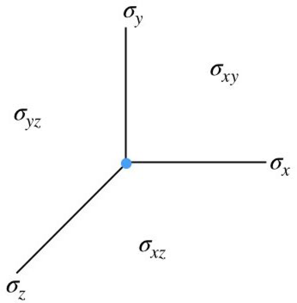
The regions $R_{\sigma _1}^{\sigma _2}$
and their corresponding
$R_{\sigma _1}^{\sigma _2}$
and their corresponding $K_{\sigma _1, \sigma _2}$
functions.
$K_{\sigma _1, \sigma _2}$
functions.
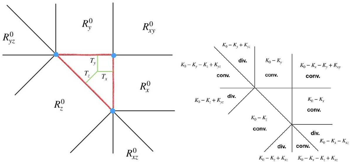
For convenience, let us write $z = x+y$
. Define the collection of functions
$z = x+y$
. Define the collection of functions $(K_\sigma )_{\sigma \in \Sigma }$
as follows.
$(K_\sigma )_{\sigma \in \Sigma }$
as follows.
-
•
$K_{xy} = K_{xz} = K_{yz} = 1$
. -
•
$K_x = K_x(y) = 1 + e^{-|y|}$
;
$K_y = K_y(x) = 1 + e^{-|x|}$
;
$K_z = K_z(x,y) = 1 + e^{-|z|}$
. -
•
$K_0 = K_0(x,y) = e^{-|z|} + e^{-|x|} + e^{-|y|}$
.


In Figure 14, we have indicated all the nonempty $R_{\sigma _1}^{\sigma _2}$
. The truncated function
$R_{\sigma _1}^{\sigma _2}$
. The truncated function $k_\Delta $
is the sum of the functions in the various regions indicated. A simple calculation shows that there are four regions where the integral of
$k_\Delta $
is the sum of the functions in the various regions indicated. A simple calculation shows that there are four regions where the integral of $|k_\Delta |$
is divergent. These regions are precisely those that are not of the form
$|k_\Delta |$
is divergent. These regions are precisely those that are not of the form $R_{\sigma _1}^{\sigma _2}$
in this example, whereas on the other regions, the hypotheses of Theorem 3.5 clearly hold. As it is evident from this example, the crucial Lemma 3.3 fails, which leads to the failure of Theorem 3.5 without the acute assumption.
$R_{\sigma _1}^{\sigma _2}$
in this example, whereas on the other regions, the hypotheses of Theorem 3.5 clearly hold. As it is evident from this example, the crucial Lemma 3.3 fails, which leads to the failure of Theorem 3.5 without the acute assumption.
We also prove the following lemma for later use in Section 4. Let $\tau $
be a cone in
$\tau $
be a cone in $\Sigma $
. Recall from Section 2.3 that
$\Sigma $
. Recall from Section 2.3 that $\Sigma / \tau $
denotes the fan consisting of all the images of the cones
$\Sigma / \tau $
denotes the fan consisting of all the images of the cones $\sigma \succeq \tau $
in the quotient vector space
$\sigma \succeq \tau $
in the quotient vector space $V / \operatorname {Span}(\tau ) \cong \tau ^\perp $
. For
$V / \operatorname {Span}(\tau ) \cong \tau ^\perp $
. For $\sigma \succeq \tau $
, let us denote the image of
$\sigma \succeq \tau $
, let us denote the image of $\sigma $
in
$\sigma $
in $V / \operatorname {Span}(\tau )$
by
$V / \operatorname {Span}(\tau )$
by $\bar {\sigma }$
. Note that by assumption, for any
$\bar {\sigma }$
. Note that by assumption, for any $\sigma \succeq \tau $
, the function
$\sigma \succeq \tau $
, the function $K_\sigma $
is constant along
$K_\sigma $
is constant along $\operatorname {Span}(\tau )$
and hence induces a well-defined function
$\operatorname {Span}(\tau )$
and hence induces a well-defined function $\bar {K}_{\bar {\sigma }}$
on
$\bar {K}_{\bar {\sigma }}$
on $V / \operatorname {Span}(\tau )$
.
$V / \operatorname {Span}(\tau )$
.
Lemma 3.7 Suppose the conditions in Theorem 3.5 for convergence are satisfied for the $K_\sigma $
,
$K_\sigma $
, $\sigma \in \Sigma $
. Then, for any
$\sigma \in \Sigma $
. Then, for any $\tau \in \Sigma $
, these conditions are also satisfied for the
$\tau \in \Sigma $
, these conditions are also satisfied for the $\bar {K}_{\bar {\sigma }}$
,
$\bar {K}_{\bar {\sigma }}$
, $\bar {\sigma } \in \Sigma / \tau $
, and hence
$\bar {\sigma } \in \Sigma / \tau $
, and hence $J_{\Sigma /\tau }(0)$
is convergent as well.
$J_{\Sigma /\tau }(0)$
is convergent as well.
Proof This is an immediate corollary of the following two observations. Let $\tau \preceq \sigma _2 \preceq \sigma _1$
. Then we have that (1) the cone
$\tau \preceq \sigma _2 \preceq \sigma _1$
. Then we have that (1) the cone $\mathcal {S}^{\bar {\sigma }_1}_{\bar {\sigma }_2}$
(as in the proof of Theorem 3.4) coincides with the image of
$\mathcal {S}^{\bar {\sigma }_1}_{\bar {\sigma }_2}$
(as in the proof of Theorem 3.4) coincides with the image of $\mathcal {S}^{\sigma _1}_{\sigma _2}$
in
$\mathcal {S}^{\sigma _1}_{\sigma _2}$
in $V / \operatorname {Span}(\tau )$
and (2) the function
$V / \operatorname {Span}(\tau )$
and (2) the function $K_{\bar {\sigma }_1, \bar {\sigma }_2}$
(as in the statement of Theorem 3.4) is rapidly decreasing on a shifted neighborhood
$K_{\bar {\sigma }_1, \bar {\sigma }_2}$
(as in the statement of Theorem 3.4) is rapidly decreasing on a shifted neighborhood $\mathcal {S}^{\bar {\sigma }_1}_{\bar {\sigma }_2}$
because
$\mathcal {S}^{\bar {\sigma }_1}_{\bar {\sigma }_2}$
because $K_{\sigma _1, \sigma _2}$
is rapidly decreasing on a shifted neighborhood of
$K_{\sigma _1, \sigma _2}$
is rapidly decreasing on a shifted neighborhood of $\mathcal {S}^{\sigma _1}_{\sigma _2}$
.▪
$\mathcal {S}^{\sigma _1}_{\sigma _2}$
.▪
Finally, we give a discrete version of Theorem 3.5. As usual, let N and M be dual lattices, and let $V=N_{\mathbb R}=N \otimes {\mathbb R}$
and
$V=N_{\mathbb R}=N \otimes {\mathbb R}$
and $V^*=M_{\mathbb R} =M \otimes {\mathbb R}$
be the corresponding vector spaces, respectively. We fix a perfect pairing
$V^*=M_{\mathbb R} =M \otimes {\mathbb R}$
be the corresponding vector spaces, respectively. We fix a perfect pairing $N \times N \to {\mathbb Z}$
and use it to identify N and M as well as
$N \times N \to {\mathbb Z}$
and use it to identify N and M as well as $N_{\mathbb R}$
and
$N_{\mathbb R}$
and $M_{\mathbb R}$
.
$M_{\mathbb R}$
.
Theorem 3.8 With the notations and assumptions as in Theorem 3.5, the sum
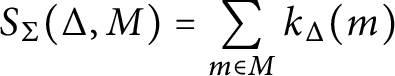 $$ \begin{align*} S_{\Sigma}(\Delta, M) = \sum_{m \in M} k_\Delta(m)\end{align*} $$
is absolutely convergent.
Proof In the proof of Theorem 3.5, replace all integrals $\int \limits _A f(x)dx$
with sums
$\int \limits _A f(x)dx$
with sums $\sum \limits _{m \in A \cap M} f(m)$
.▪
$\sum \limits _{m \in A \cap M} f(m)$
.▪
We should note that the discrete analogue of Lemma 3.7 also holds with the same proof.
4 Polynomiality
In this section, we prove the following theorems.
Theorem 4.1 (Polynomiality)
Let $\Sigma $
be a full dimensional, complete, simplicial fan in V which is assumed to be acute. Let
$\Sigma $
be a full dimensional, complete, simplicial fan in V which is assumed to be acute. Let $(K_\sigma )_{\sigma \in \Sigma }$
be a collection of continuous functions satisfying the assumptions (i) and (ii) in Theorem 3.5. Then
$(K_\sigma )_{\sigma \in \Sigma }$
be a collection of continuous functions satisfying the assumptions (i) and (ii) in Theorem 3.5. Then
 $$ \begin{align*} J_{\Sigma}(\Delta) = \int\limits_V k_\Delta(x) dx \end{align*} $$
is a polynomial function on ${\mathcal P}(\Sigma )$
, i.e., a polynomial in the support numbers of
${\mathcal P}(\Sigma )$
, i.e., a polynomial in the support numbers of $\Delta $
.
$\Delta $
.
We also prove a discrete version of the above polynomiality result. Let N and M be dual lattices with $V=N_{\mathbb R}$
and
$V=N_{\mathbb R}$
and $V^*=M_{\mathbb R}$
the corresponding vector spaces. We fix a perfect
$V^*=M_{\mathbb R}$
the corresponding vector spaces. We fix a perfect ${\mathbb Z}$
-pairing
${\mathbb Z}$
-pairing $N \times N \to {\mathbb Z}$
and use it to identify N and M. Recall that
$N \times N \to {\mathbb Z}$
and use it to identify N and M. Recall that ${\mathcal P}(\Sigma , M)$
denotes the collection of polytopes with normal fan
${\mathcal P}(\Sigma , M)$
denotes the collection of polytopes with normal fan $\Sigma $
whose vertices lie in M.
$\Sigma $
whose vertices lie in M.
Theorem 4.2 Let the notations and assumptions be as in Theorem 4.1. Then
 $$\begin{align*}S_{\Sigma}(\Delta) = \sum_{m \in M} k_\Delta(m) \end{align*}$$
is a polynomial function on ${\mathcal P}(\Sigma , M)$
.
${\mathcal P}(\Sigma , M)$
.
A key step in the proof of Theorem 4.1 is a combinatorial lemma (Lemma 4.6) which we deduce as a corollary of the Lawrence–Varchenko conical decomposition (Theorem 2.10). The notion of a virtual polytope naturally appears here (see Section 2.6). The proof of Theorem 4.2 is a slight modification of the proof of Theorem 4.1. We give the proofs in Section 4.2 below after some preparation. Let us give some examples first.
Example 4.3 (Brianchon–Gram)
Let $\Sigma $
be a simplicial fan in V with
$\Sigma $
be a simplicial fan in V with $\Delta \in \mathcal {P}(\Sigma )$
a polytope normal to
$\Delta \in \mathcal {P}(\Sigma )$
a polytope normal to $\Sigma $
. Let
$\Sigma $
. Let $K_\sigma \equiv 1$
and
$K_\sigma \equiv 1$
and $\forall \sigma \in \Sigma $
. The combinatorial truncation
$\forall \sigma \in \Sigma $
. The combinatorial truncation $k_\Delta $
in this case is given by
$k_\Delta $
in this case is given by
 $$ \begin{align*}k_\Delta = \sum_{\sigma \in \Sigma} (-1)^{\dim(\sigma)} {\textbf 1}_{T^-_{\Delta, \sigma}}.\end{align*} $$
By the Brianchon–Gram theorem (Theorem 2.7), we have
 $$ \begin{align*} k_\Delta = {\textbf 1}_{\Delta}. \end{align*} $$
For any pair of cones $\sigma _1 \preceq \sigma _2$
in
$\sigma _1 \preceq \sigma _2$
in $\Sigma $
, we have
$\Sigma $
, we have
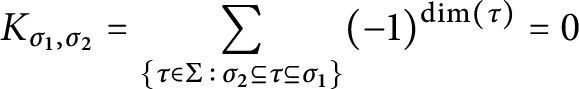 $$ \begin{align*} K_{\sigma_1, \sigma_2} = \sum_{\left\{\tau\in\Sigma \, : \, \sigma_2 \subseteq \tau \subseteq \sigma_1 \right\}} (-1)^{\dim(\tau)} = 0 \end{align*} $$
by the binomial identity $\sum _{k=0}^n (-1)^k {n \choose k} = 0$
. Thus, the conditions in Theorem 3.5 are satisfied. Moreover, the
$\sum _{k=0}^n (-1)^k {n \choose k} = 0$
. Thus, the conditions in Theorem 3.5 are satisfied. Moreover, the $K_\sigma $
are constant, and hence the assumptions in the polynomiality theorem are also satisfied. Thus, we recover the polynomiality of the volume function
$K_\sigma $
are constant, and hence the assumptions in the polynomiality theorem are also satisfied. Thus, we recover the polynomiality of the volume function $\Delta \mapsto \operatorname {vol}(\Delta )$
(see Theorem 2.1).
$\Delta \mapsto \operatorname {vol}(\Delta )$
(see Theorem 2.1).
Example 4.4 (Rectangle)
We consider the fan $\Sigma $
in
$\Sigma $
in $V ={\mathbb R}^2$
as in Figure 15, consisting of one-dimensional cones
$V ={\mathbb R}^2$
as in Figure 15, consisting of one-dimensional cones $\sigma _x$
and
$\sigma _x$
and $\sigma _y$
and their opposites, as well as the two-dimensional cone
$\sigma _y$
and their opposites, as well as the two-dimensional cone $\sigma _{xy}$
and its counterparts for the other three quadrants. We also have the cone
$\sigma _{xy}$
and its counterparts for the other three quadrants. We also have the cone $\{0\}$
. The fan
$\{0\}$
. The fan $\Sigma $
is normal to the rectangle
$\Sigma $
is normal to the rectangle $\Delta $
with support numbers
$\Delta $
with support numbers $T_1, T_2, T^{\prime }_1, T^{\prime }_2$
as indicated.
$T_1, T_2, T^{\prime }_1, T^{\prime }_2$
as indicated.
Illustration of the truncated function $k_\Delta $
for when
$k_\Delta $
for when $\Delta $
is a rectangle.
$\Delta $
is a rectangle.
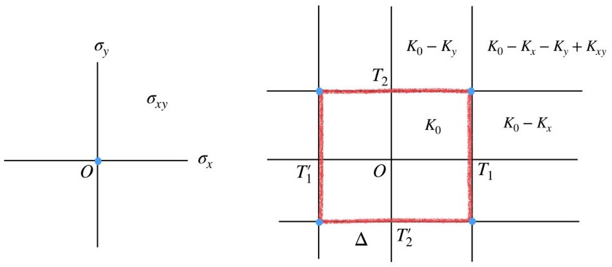
Let $f(x,y)$
be an absolutely integrable function on
$f(x,y)$
be an absolutely integrable function on ${\mathbb R}^2$
with
${\mathbb R}^2$
with $f_{++}$
denoting the value of its integral over the first quadrant. Similarly, let the values of its integral over the other quadrants be denoted by
$f_{++}$
denoting the value of its integral over the first quadrant. Similarly, let the values of its integral over the other quadrants be denoted by $f_{+-}$
,
$f_{+-}$
, $f_{-+}$
,
$f_{-+}$
, $f_{--}$
. Also, let
$f_{--}$
. Also, let $g(x)$
and
$g(x)$
and $h(y)$
be absolutely integrable functions on
$h(y)$
be absolutely integrable functions on ${\mathbb R}$
with their integrals over
${\mathbb R}$
with their integrals over $[0,\infty )$
denoted by
$[0,\infty )$
denoted by $g_+$
and
$g_+$
and $h_+$
and their integrals over
$h_+$
and their integrals over $(-\infty ,0]$
denoted by
$(-\infty ,0]$
denoted by $g_-$
and
$g_-$
and $h_-$
, respectively. Finally, let k denote a constant.
$h_-$
, respectively. Finally, let k denote a constant.
We assign the following functions to the cones in $\Sigma $
:
$\Sigma $
:
-
•
$K_0(x, y) = f(x,y) + g(x) + h(y) + k$
, -
•
$K_{\sigma _{\pm x}}(x,y) = h(y) + k$
, -
•
$K_{\sigma _{\pm y}}(x,y) = g(x) + k$
, and -
•
$K_\sigma (x,y) = k$
for all two-dimensional cones
$\sigma $
in
$\Sigma $
.


Notice that the conditions (i) and (ii) of Theorem 3.5 are clearly satisfied.
Let us calculate $J_{\Sigma }(\Delta )$
. Because of the symmetry in this example, it is enough to consider a quarter of the picture. We have
$J_{\Sigma }(\Delta )$
. Because of the symmetry in this example, it is enough to consider a quarter of the picture. We have
 $$ \begin{align*} & \int_0^{T_1} \int_0^{T_2} \left(f(x,y) + g(x) + h(y) + k\right) \, dy \, dx + \int_0^{T_1} \int_{T_2}^{\infty} \left(f(x,y)+h(y)\right) \, dy \, dx \\ &\quad + \int_{T_1}^{\infty} \int_{0}^{T_2} \left(f(x,y) + g(x)\right) \, dy \, dx + \int_{T_1}^{\infty} \int_{T_2}^{\infty} f(x,y) \, dy \, dx \\ &= f_{++} + g_+ T_2 + h_+ T_1 + k T_1 T_2, \end{align*} $$
which is a polynomial of degree $2$
in
$2$
in $T_1$
and
$T_1$
and $T_2$
. Adding similar contributions from the other three quadrants, we arrive at
$T_2$
. Adding similar contributions from the other three quadrants, we arrive at
 $$\begin{align*}J_{\Sigma}(\Delta) &= k \, (T_1 + T^{\prime}_1) (T_2 + T^{\prime}_2) + h_+ \, T_1 + g_- \, T^{\prime}_1 + g_+ \, T_2 + g_- \, T^{\prime}_2\\ &\quad + (f_{++} + f_{+-} + f_{-+} + f_{--}). \end{align*}$$
4.1 An extension of the Langlands combinatorial lemma
As before, V is an n-dimensional real vector space. We fix an inner product $\langle \cdot , \cdot \rangle $
on V and identify V with its dual space
$\langle \cdot , \cdot \rangle $
on V and identify V with its dual space $V^*$
. Let
$V^*$
. Let $\Sigma $
be a full dimensional, complete, simplicial fan in V, and let
$\Sigma $
be a full dimensional, complete, simplicial fan in V, and let $\Delta \in \mathcal {P}(\Sigma )$
be a full dimensional simple polytope with normal fan
$\Delta \in \mathcal {P}(\Sigma )$
be a full dimensional simple polytope with normal fan $\Sigma $
. Since we identified V and
$\Sigma $
. Since we identified V and $V^*$
, we take both
$V^*$
, we take both $\Sigma $
and
$\Sigma $
and $\Delta $
to lie in V.
$\Delta $
to lie in V.
Let $\sigma \in \Sigma $
be a cone. First, we consider the case where
$\sigma \in \Sigma $
be a cone. First, we consider the case where $\sigma $
is full dimensional. Let
$\sigma $
is full dimensional. Let $v_\sigma $
be the corresponding vertex of
$v_\sigma $
be the corresponding vertex of $\Delta $
. Let
$\Delta $
. Let $W = \{w_1, \ldots , w_n\}$
(resp.
$W = \{w_1, \ldots , w_n\}$
(resp. $B = \{b_1, \ldots , b_n\}$
) be the set of edge vectors of
$B = \{b_1, \ldots , b_n\}$
) be the set of edge vectors of $\sigma $
(resp. of
$\sigma $
(resp. of $\sigma ^\vee $
). Then the
$\sigma ^\vee $
). Then the $b_i$
(resp. the
$b_i$
(resp. the $w_j$
) are the inward facet normals to
$w_j$
) are the inward facet normals to $\sigma $
(resp.
$\sigma $
(resp. $\sigma ^\vee $
), and the cone
$\sigma ^\vee $
), and the cone $\sigma $
is given by inequalities as
$\sigma $
is given by inequalities as
 $$\begin{align*}\sigma = \left\{ x : \langle x, b_i \rangle \geqslant0,~i=1, \ldots, n \right\}. \end{align*}$$
Also, the inward-looking tangent cone $T^+_{\Delta , \sigma }$
at the vertex
$T^+_{\Delta , \sigma }$
at the vertex $v_\sigma $
is given by
$v_\sigma $
is given by
 $$\begin{align*}T^+_{\Delta, \sigma} = \left\{ x : \langle x, w_i \rangle \leqslant \langle v_\sigma, w_i \rangle,~ i=1, \ldots, n \right\}. \end{align*}$$
We consider the oriented hyperplanes corresponding to the union of these two sets of inequalities:
 $$ \begin{align} H_{b_i, 0} &= \left\{x : \langle x, b_i \rangle = 0 \right\}, & i=1, \ldots, n, \nonumber \\ H_{w_i, \langle v_\sigma, w \rangle} &= \left\{x : \langle x, w_i \rangle = \langle v_\sigma, w \rangle \right\}, & i=1, \ldots, n. \end{align} $$
If $v_\sigma $
lies in
$v_\sigma $
lies in $\sigma $
, then the hyperplanes in (4.1) are the facets of the polytope
$\sigma $
, then the hyperplanes in (4.1) are the facets of the polytope $\Delta \cap \sigma $
oriented outward. In general,
$\Delta \cap \sigma $
oriented outward. In general, $v_\sigma $
may not lie in
$v_\sigma $
may not lie in $\sigma $
.
$\sigma $
.
Definition 4.1 We denote the virtual polytope in V determined by the oriented hyperplanes in (4.1) by $\Gamma _{\Delta , \sigma }$
. We denote the convex chain corresponding to
$\Gamma _{\Delta , \sigma }$
. We denote the convex chain corresponding to $\Gamma _{\Delta , \sigma }$
by
$\Gamma _{\Delta , \sigma }$
by $\gamma _{\Delta , \sigma }$
.
$\gamma _{\Delta , \sigma }$
.
See Section 2.6 for a review of the notions of virtual polytope and convex chain. Also, see Figure 16 for a three-dimensional example of $\Gamma _{\Delta ,\sigma }$
and Figure 17 for a pair of two-dimensional examples of the virtual polytope
$\Gamma _{\Delta ,\sigma }$
and Figure 17 for a pair of two-dimensional examples of the virtual polytope $\Gamma _{\Delta , \sigma }$
and its convex chain
$\Gamma _{\Delta , \sigma }$
and its convex chain $\gamma _{\Delta , \sigma }$
.
$\gamma _{\Delta , \sigma }$
.
A three-dimensional example where $\Gamma _{\Delta , \sigma }$
is a cube. A face
$\Gamma _{\Delta , \sigma }$
is a cube. A face $\tau $
(of
$\tau $
(of $\sigma $
) and its corresponding dual face
$\sigma $
) and its corresponding dual face $\tau ^*$
(of
$\tau ^*$
(of $\sigma ^\vee $
) and the vertex
$\sigma ^\vee $
) and the vertex $v_\tau $
(of
$v_\tau $
(of $\Gamma _{\Delta , \sigma }$
) are illustrated.
$\Gamma _{\Delta , \sigma }$
) are illustrated.
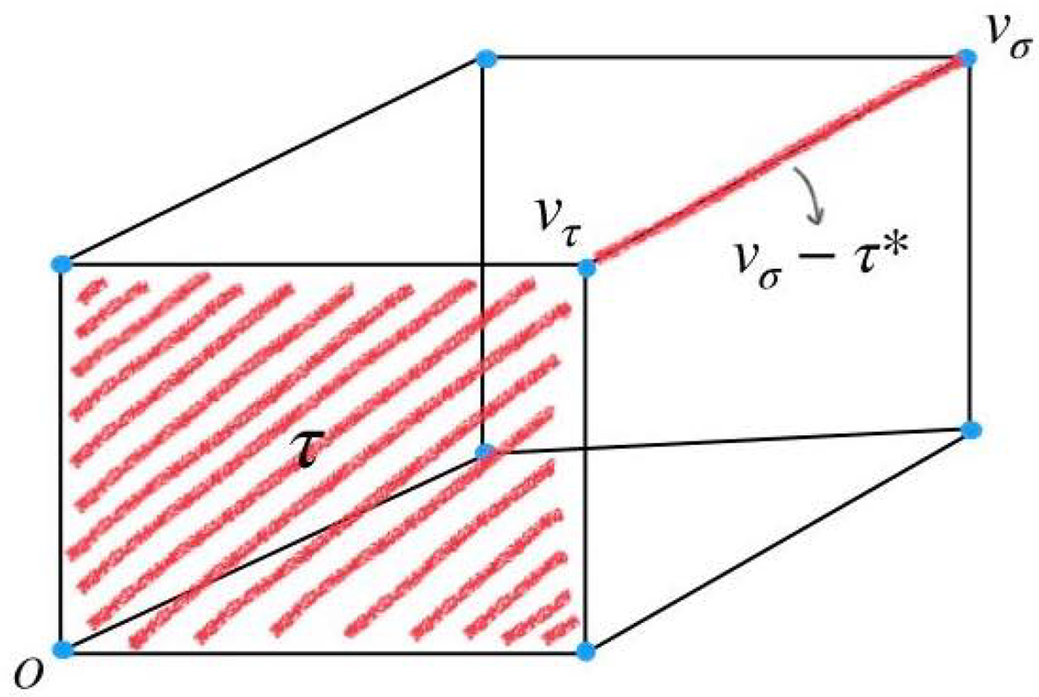
Two examples of the virtual polytopes $\Gamma _{\Delta , \sigma }$
. In the first example, the vertex
$\Gamma _{\Delta , \sigma }$
. In the first example, the vertex $v_\sigma $
lies in the cone
$v_\sigma $
lies in the cone $\sigma $
and
$\sigma $
and $\Gamma _{\Delta , \sigma }$
is an actual polytope (a quadrangle). The convex chain
$\Gamma _{\Delta , \sigma }$
is an actual polytope (a quadrangle). The convex chain $\gamma _{\Delta , \sigma }$
is the characteristic function of the quadrangle. In the second example,
$\gamma _{\Delta , \sigma }$
is the characteristic function of the quadrangle. In the second example, $v_\sigma $
lies outside
$v_\sigma $
lies outside $\sigma $
and
$\sigma $
and $\Gamma _{\Delta , \sigma }$
is a virtual quadrangle. The convex chain
$\Gamma _{\Delta , \sigma }$
is a virtual quadrangle. The convex chain $\gamma _{\Delta , \sigma }$
is the function which has values
$\gamma _{\Delta , \sigma }$
is the function which has values $1$
and
$1$
and $-1$
in the two shaded regions, respectively.
$-1$
in the two shaded regions, respectively.
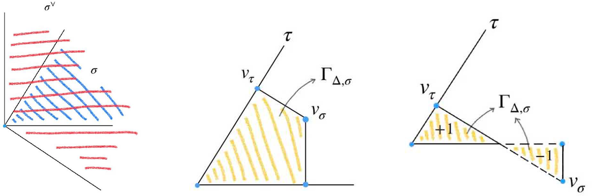
In this section, we consider the Lawrence–Varchenko conical decomposition for the virtual polytope $\Gamma _{\Delta , \sigma }$
(Theorem 2.10). We will see that this recovers and extends some of the key combinatorial lemmas appearing in Arthur’s work (e.g., [Reference ArthurAr81]). As a special case, we immediately recover the Langlands combinatorial lemma (see [Reference ArthurAr05, Section I.8, p. 46], [Reference Goresky, Kottwitz and MacPhersonGKM97, Appendix B]). In addition, we interpret the Langlands combinatorial lemma as a formula for the inverse of a distinguished element in the incidence algebra of poset of faces of
$\Gamma _{\Delta , \sigma }$
(Theorem 2.10). We will see that this recovers and extends some of the key combinatorial lemmas appearing in Arthur’s work (e.g., [Reference ArthurAr81]). As a special case, we immediately recover the Langlands combinatorial lemma (see [Reference ArthurAr05, Section I.8, p. 46], [Reference Goresky, Kottwitz and MacPhersonGKM97, Appendix B]). In addition, we interpret the Langlands combinatorial lemma as a formula for the inverse of a distinguished element in the incidence algebra of poset of faces of $\sigma $
(see Section 2.7).
$\sigma $
(see Section 2.7).
Recall that for $\tau \preceq \sigma $
, the largest face of
$\tau \preceq \sigma $
, the largest face of $\sigma ^\vee $
orthogonal to
$\sigma ^\vee $
orthogonal to $\tau $
is denoted by
$\tau $
is denoted by $\tau ^*$
and we have
$\tau ^*$
and we have $\dim \tau + \dim \tau ^* = n$
(Section 2.1). It follows that the intersection
$\dim \tau + \dim \tau ^* = n$
(Section 2.1). It follows that the intersection $\operatorname {Span}(\tau ) \cap (v_\sigma + \operatorname {Span}(\tau ^*))$
is a single point which can be shown to be a vertex
$\operatorname {Span}(\tau ) \cap (v_\sigma + \operatorname {Span}(\tau ^*))$
is a single point which can be shown to be a vertex $v_\tau $
of
$v_\tau $
of $\Gamma _{\Delta , \sigma }$
. In fact, we will see below that
$\Gamma _{\Delta , \sigma }$
. In fact, we will see below that $\tau \mapsto v_\tau $
gives a one-to-one correspondence between the faces of
$\tau \mapsto v_\tau $
gives a one-to-one correspondence between the faces of $\sigma $
and the vertices of
$\sigma $
and the vertices of $\Gamma _{\Delta , \sigma }$
. The vertex corresponding to the zero-dimensional face
$\Gamma _{\Delta , \sigma }$
. The vertex corresponding to the zero-dimensional face $0$
is
$0$
is $0$
itself. On the other hand, the vertex corresponding to the whole
$0$
itself. On the other hand, the vertex corresponding to the whole $\sigma $
is the vertex
$\sigma $
is the vertex $v_\sigma $
of
$v_\sigma $
of $\Delta $
.
$\Delta $
.
For a face $\tau \preceq \sigma $
, let
$\tau \preceq \sigma $
, let $W(\tau ) \subset W$
(resp.
$W(\tau ) \subset W$
(resp. $B(\tau ) \subset B$
) be the subset of edge vectors of
$B(\tau ) \subset B$
) be the subset of edge vectors of $\tau $
(resp.
$\tau $
(resp. $\tau ^*$
). Thus,
$\tau ^*$
). Thus,
 $$ \begin{align*} \tau = \{ x \in \sigma : \langle x, b \rangle = 0,~ b \in B(\tau) \}. \end{align*} $$
The vertex $v_\tau $
is then the unique solution of the system of equations
$v_\tau $
is then the unique solution of the system of equations
 $$\begin{align*}\begin{cases} \langle x, w \rangle = \langle v_\sigma, w \rangle, & \forall w \in W(\tau), \\ \langle x, b \rangle = 0, & \forall b \in B(\tau). \\ \end{cases} \end{align*}$$
Moreover, the inward tangent cone $T^+_{\Gamma _{\Delta , \sigma }, v_\tau }$
at the vertex
$T^+_{\Gamma _{\Delta , \sigma }, v_\tau }$
at the vertex $v_\tau $
is given by the inequalities
$v_\tau $
is given by the inequalities
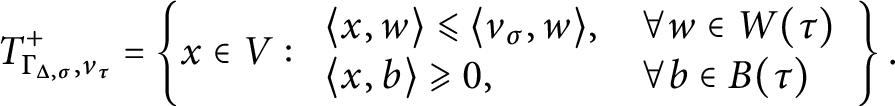 $$\begin{align*}T^+_{\Gamma_{\Delta, \sigma}, v_\tau} = \left\{x \in V : \begin{array}{ll} \langle x, w \rangle \leqslant \langle v_\sigma, w \rangle, & \forall w \in W(\tau) \\ \langle x, b \rangle \geqslant0, & \forall b \in B(\tau) \end{array} \right\}. \end{align*}$$
Thus, the set of outward facet normals of $\Gamma _{\Delta , \sigma }$
at
$\Gamma _{\Delta , \sigma }$
at $v_\tau $
is
$v_\tau $
is $W(\tau ) \cup -B(\tau )$
. In other words, the cone in the normal fan of
$W(\tau ) \cup -B(\tau )$
. In other words, the cone in the normal fan of $\Gamma _{\Delta , \sigma }$
corresponding to the vertex
$\Gamma _{\Delta , \sigma }$
corresponding to the vertex $v_\tau $
is generated by the set of vectors
$v_\tau $
is generated by the set of vectors $W(\tau ) \cup -B(\tau )$
(Section 2.3).
$W(\tau ) \cup -B(\tau )$
(Section 2.3).
Consider the nearest face partition corresponding to $\sigma $
(Section 2.4). That is, for each face
$\sigma $
(Section 2.4). That is, for each face $\tau $
, let
$\tau $
, let $V_\sigma ^\tau $
be the set of points
$V_\sigma ^\tau $
be the set of points $x \in V$
whose shortest distance to
$x \in V$
whose shortest distance to $\sigma $
is attained at a point in the relative interior of
$\sigma $
is attained at a point in the relative interior of $\tau $
. Since
$\tau $
. Since $\sigma $
is a cone, each
$\sigma $
is a cone, each $V_\sigma ^\tau $
is a full dimensional cone. Moreover, the closures of the cones
$V_\sigma ^\tau $
is a full dimensional cone. Moreover, the closures of the cones $V_\sigma ^\tau $
,
$V_\sigma ^\tau $
, $\tau \preceq \sigma $
, are the maximal cones of a complete simplicial fan in V which we call the nearest face fan of
$\tau \preceq \sigma $
, are the maximal cones of a complete simplicial fan in V which we call the nearest face fan of $\sigma $
. The following is straightforward to verify.
$\sigma $
. The following is straightforward to verify.
Proposition 4.5 In the nearest face fan of $\sigma $
, the cone corresponding to a face
$\sigma $
, the cone corresponding to a face $\tau \preceq \sigma $
is the convex cone generated by the set of vectors
$\tau \preceq \sigma $
is the convex cone generated by the set of vectors $W(\tau ) \cup -B(\tau )$
.
$W(\tau ) \cup -B(\tau )$
.
Since the $V_\sigma ^\tau $
partition of the whole space V, the above proposition shows that the union of the cones generated by
$V_\sigma ^\tau $
partition of the whole space V, the above proposition shows that the union of the cones generated by $W(\tau ) \cup -B(\tau )$
,
$W(\tau ) \cup -B(\tau )$
, $\tau \preceq \sigma $
, is V. This then implies that the normal fan of
$\tau \preceq \sigma $
, is V. This then implies that the normal fan of $\Gamma _{\Delta , \sigma }$
coincides with the nearest fan of
$\Gamma _{\Delta , \sigma }$
coincides with the nearest fan of $\sigma $
. In particular, the
$\sigma $
. In particular, the $v_\tau $
are all of the vertices of
$v_\tau $
are all of the vertices of $\Gamma _{\Delta , \sigma }$
. In other words,
$\Gamma _{\Delta , \sigma }$
. In other words, $\tau \mapsto v_\tau $
gives a one-to-one correspondence between the faces of
$\tau \mapsto v_\tau $
gives a one-to-one correspondence between the faces of $\sigma $
and the vertices of
$\sigma $
and the vertices of $\Gamma _{\Delta , \sigma }$
.
$\Gamma _{\Delta , \sigma }$
.
Now, take a vector $\xi $
in
$\xi $
in $\sigma ^\circ \cap (\sigma ^\vee )^\circ $
, that is,
$\sigma ^\circ \cap (\sigma ^\vee )^\circ $
, that is,
 $$ \begin{align*} \langle \xi, b \rangle> 0,~ \forall b \in B, \end{align*} $$
 $$ \begin{align*} \langle \xi, w \rangle> 0,~ \forall w \in W. \end{align*} $$
Note that since $\sigma \neq V$
, we know
$\sigma \neq V$
, we know $(\sigma ^\circ )^\vee + \sigma ^\circ \neq V$
and hence
$(\sigma ^\circ )^\vee + \sigma ^\circ \neq V$
and hence $\sigma ^\circ \cap (\sigma ^\vee )^\circ = ((\sigma ^\circ )^\vee + \sigma ^\circ )^\vee \neq \emptyset $
.
$\sigma ^\circ \cap (\sigma ^\vee )^\circ = ((\sigma ^\circ )^\vee + \sigma ^\circ )^\vee \neq \emptyset $
.
Let $T^\xi _{\Gamma _{\Delta , \sigma }, v_\tau }$
be the polarized tangent cone at the vertex
$T^\xi _{\Gamma _{\Delta , \sigma }, v_\tau }$
be the polarized tangent cone at the vertex $v_\tau $
appearing in the Lawrence–Varchenko decomposition of
$v_\tau $
appearing in the Lawrence–Varchenko decomposition of $\Gamma _{\Delta , \sigma }$
relative to the vector
$\Gamma _{\Delta , \sigma }$
relative to the vector $\xi $
(see Section 2.5). By construction, the edge vectors of
$\xi $
(see Section 2.5). By construction, the edge vectors of $T^\xi _{\Gamma _{\Delta , \sigma }, v_\tau }$
are
$T^\xi _{\Gamma _{\Delta , \sigma }, v_\tau }$
are $\pm $
the edge vectors of the tangent cone of
$\pm $
the edge vectors of the tangent cone of $\Gamma _{\Delta , \sigma }$
at
$\Gamma _{\Delta , \sigma }$
at $v_\tau $
so that the minimum of
$v_\tau $
so that the minimum of $\langle \xi , \cdot \rangle $
on
$\langle \xi , \cdot \rangle $
on $T^\xi _{\Gamma _{\Delta , \sigma }, v_\tau }$
is attained at the vertex
$T^\xi _{\Gamma _{\Delta , \sigma }, v_\tau }$
is attained at the vertex $v_\tau $
. Since the inner product of
$v_\tau $
. Since the inner product of $\xi $
with any vector in
$\xi $
with any vector in $W \cup B$
is positive, it follows that the set of inward facet normals of
$W \cup B$
is positive, it follows that the set of inward facet normals of $T^\xi _{\Gamma _{\Delta , \sigma }, v_\tau }$
is exactly
$T^\xi _{\Gamma _{\Delta , \sigma }, v_\tau }$
is exactly $W(\tau ) \cup B(\tau )$
. More precisely,
$W(\tau ) \cup B(\tau )$
. More precisely, $T^\xi _{\Gamma _{\Delta , \sigma }, v_\tau }$
is defined by the inequalities
$T^\xi _{\Gamma _{\Delta , \sigma }, v_\tau }$
is defined by the inequalities
 $$ \begin{align} T^\xi_{\Gamma_{\Delta, \sigma}, v_\tau} = \left\{ x \in V : \begin{array}{ll} \langle x, w \rangle> \langle v_\sigma, w \rangle, & \forall w \in W(\tau) \\ \langle x, b \rangle \geqslant 0, & \forall b \in B(\tau) \end{array} \right\}. \end{align} $$
On the other hand, let $C_\sigma ^\tau $
be the inward-looking tangent cone of
$C_\sigma ^\tau $
be the inward-looking tangent cone of $\sigma $
at
$\sigma $
at $\tau $
. It is the cone defined as
$\tau $
. It is the cone defined as
 $$ \begin{align*} C_\sigma^\tau = \{ x \in V : \langle x, b \rangle \geqslant 0,~\forall b \in B(\tau)\}. \end{align*} $$
It follows from (4.2) that $T^\xi _{\Gamma _{\Delta , \sigma }, v_\tau }$
can be written as
$T^\xi _{\Gamma _{\Delta , \sigma }, v_\tau }$
can be written as
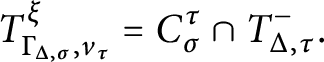 $$ \begin{align*} T^\xi_{\Gamma_{\Delta, \sigma}, v_\tau} = C_\sigma^\tau \cap T^-_{\Delta, \tau}. \end{align*} $$
If $\sigma $
is not full dimensional, we can repeat the above, replacing
$\sigma $
is not full dimensional, we can repeat the above, replacing $\Delta $
with
$\Delta $
with $\Delta \cap \operatorname {Span}(\sigma )$
. Then
$\Delta \cap \operatorname {Span}(\sigma )$
. Then $\gamma _{\Delta , \sigma }$
is a convex chain supported on
$\gamma _{\Delta , \sigma }$
is a convex chain supported on $\operatorname {Span}(\sigma )$
. We extend
$\operatorname {Span}(\sigma )$
. We extend $\gamma _{\Delta , \sigma }$
to the whole V by requiring it to be constant along
$\gamma _{\Delta , \sigma }$
to the whole V by requiring it to be constant along $\sigma ^\perp $
. Now, applying the Lawrence–Varchenko theorem to the virtual polytope
$\sigma ^\perp $
. Now, applying the Lawrence–Varchenko theorem to the virtual polytope $\Gamma _{\Delta , \sigma }$
and the vector
$\Gamma _{\Delta , \sigma }$
and the vector $\xi $
as above, we obtain the following conical decomposition for
$\xi $
as above, we obtain the following conical decomposition for $\Gamma _{\Delta , \sigma }$
.
$\Gamma _{\Delta , \sigma }$
.
Lemma 4.6 With notation as above, let $\gamma _{\Delta , \sigma }$
be the convex chain associated with
$\gamma _{\Delta , \sigma }$
be the convex chain associated with
the virtual polytope $\Gamma _{\Delta , \sigma }$
. We have
$\Gamma _{\Delta , \sigma }$
. We have
 $$ \begin{align} \gamma_{\Delta, \sigma} = \sum_{\tau \preceq \sigma} (-1)^{\dim \tau} {\textbf 1}_{C_\sigma^\tau} {\textbf 1}_{T^-_{\Delta, \tau}}. \end{align} $$
Proof First, we note that the number $n_{v_\tau }$
of the edges flipped in the polarized tangent cone
$n_{v_\tau }$
of the edges flipped in the polarized tangent cone $T^\xi _{\Gamma _{\Delta , \sigma }, v_\tau }$
is equal to
$T^\xi _{\Gamma _{\Delta , \sigma }, v_\tau }$
is equal to $|W(\tau )| = \dim \tau $
. The above discussion then proves the case where
$|W(\tau )| = \dim \tau $
. The above discussion then proves the case where $\sigma $
is full dimensional. If
$\sigma $
is full dimensional. If $\sigma $
is not full dimensional, all the cones considered in the right-hand side of (4.3) above should be extended in the orthogonal direction
$\sigma $
is not full dimensional, all the cones considered in the right-hand side of (4.3) above should be extended in the orthogonal direction $\sigma ^\perp $
. This finishes the proof.▪
$\sigma ^\perp $
. This finishes the proof.▪
Letting $\Delta = \{0\}$
, we recover a combinatorial lemma of Langlands.
$\Delta = \{0\}$
, we recover a combinatorial lemma of Langlands.
Corollary 4.7 (Langlands combinatorial lemma)
Let $\sigma \subset V$
be a convex polyhedral cone. The following identities hold.
$\sigma \subset V$
be a convex polyhedral cone. The following identities hold.
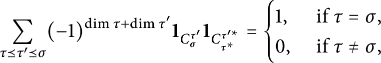 $$ \begin{align} \sum_{\tau \preceq \tau' \preceq \sigma} (-1)^{\dim \tau + \dim \tau'} {\textbf 1}_{C_\sigma^{\tau'}} {\textbf 1}_{C_{\tau^*}^{\tau^{\prime *}}} = \begin{cases} 1, & \mbox{ if } \tau = \sigma, \\ 0, & \mbox{ if } \tau \neq \sigma, \end{cases} \end{align} $$
 $$ \begin{align} \sum_{\tau \preceq \tau' \preceq \sigma} (-1)^{\dim \tau' + \dim \tau} {\textbf 1}_{C_\tau^{\tau'}} {\textbf 1}_{C_{\sigma^*}^{\tau^{\prime *}}} = \begin{cases} 1, & \mbox{ if } \tau = \sigma, \\ 0, & \mbox{ if } \tau \neq \sigma. \end{cases} \end{align} $$
Alternatively, consider the incidence algebra of the poset of faces of $\sigma $
with ring of scalars R being the ring of all real-valued functions on V (see Section 2.7 and Example 2.12
). Define the elements F and G of the incidence algebra by
$\sigma $
with ring of scalars R being the ring of all real-valued functions on V (see Section 2.7 and Example 2.12
). Define the elements F and G of the incidence algebra by
 $$ \begin{align*} F(\tau, \tau') &= (-1)^{\dim \tau} {\textbf 1}_{C_\tau^{\tau'}},\\ G(\tau, \tau') &= (-1)^{\dim \tau} {\textbf 1}_{C_{\tau^*}^{\tau^{\prime *}}}. \end{align*} $$
Equations ( 4.4 ) and ( 4.5 ) state that F and G are inverses of each other in the incidence algebra, that is,
 $$ \begin{align} (F * G)(\tau, \sigma) = (G * F)(\tau, \sigma) = \delta(\tau, \sigma). \end{align} $$
Proof First, to prove (4.4), we can assume without loss of generality that $\tau =0$
. Equation (4.4) is then an immediate consequence of (4.3) when we let
$\tau =0$
. Equation (4.4) is then an immediate consequence of (4.3) when we let $\Delta = \{0\}$
. To obtain (4.5), we apply (4.4) to
$\Delta = \{0\}$
. To obtain (4.5), we apply (4.4) to $\sigma ^\vee $
in place of
$\sigma ^\vee $
in place of $\sigma $
. Finally, (4.6) is a rewriting of (4.4) and (4.5) using the language of incidence algebra.▪
$\sigma $
. Finally, (4.6) is a rewriting of (4.4) and (4.5) using the language of incidence algebra.▪
Corollary 4.8 With notation as before, we have
 $$ \begin{align} {\textbf 1}_{T^-_{\Delta, \sigma}} = \sum_{\tau \preceq \sigma} (-1)^{\dim \tau} {\textbf 1}_{C_{\sigma}^{\tau}} \, \gamma_{\Delta, \tau}. \end{align} $$
Proof Let H and L be elements of the incidence algebra such that $H(0, \tau ) = {\textbf 1}_{T^-_{\Delta , \sigma }}$
and
$H(0, \tau ) = {\textbf 1}_{T^-_{\Delta , \sigma }}$
and $L(0, \tau ) = \gamma _{\Delta , \tau }$
,
$L(0, \tau ) = \gamma _{\Delta , \tau }$
, $\forall \tau \preceq \sigma $
. Then (4.3) states that
$\forall \tau \preceq \sigma $
. Then (4.3) states that $L(0, \tau ) = (H * F)(0, \tau )$
. Convolution of both sides from right with G gives
$L(0, \tau ) = (H * F)(0, \tau )$
. Convolution of both sides from right with G gives $(L * G)(0, \tau ) = H(0, \tau )$
, which is exactly (4.7).▪
$(L * G)(0, \tau ) = H(0, \tau )$
, which is exactly (4.7).▪
4.2 Proof of polynomiality
Proof of Theorem 4.1
In the definition of $J_{\Sigma }(\Delta )$
, we use Corollary 4.8 to write
$J_{\Sigma }(\Delta )$
, we use Corollary 4.8 to write $T^-_{\Delta , \sigma }$
as
$T^-_{\Delta , \sigma }$
as $\sum \limits _{\tau \preceq \sigma } (-1)^{\dim \tau } {\textbf 1}_{C_{\sigma }^{\tau }} \, \gamma _{\Delta , \tau }$
. We have
$\sum \limits _{\tau \preceq \sigma } (-1)^{\dim \tau } {\textbf 1}_{C_{\sigma }^{\tau }} \, \gamma _{\Delta , \tau }$
. We have
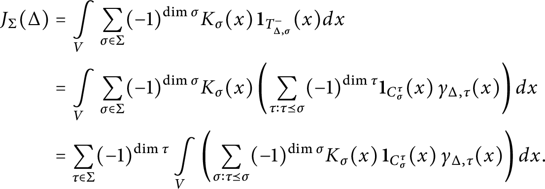 $$ \begin{align*} J_{\Sigma}(\Delta) &= \int\limits_{V} \sum_{\sigma \in \Sigma} (-1)^{\dim \sigma} K_\sigma(x) \, {\textbf 1}_{T^-_{\Delta, \sigma}}(x) dx \\ &= \int\limits_{V} \sum_{\sigma \in \Sigma} (-1)^{\dim \sigma} K_\sigma(x) \left( \sum_{\tau: \tau \preceq \sigma} (-1)^{\dim \tau} {\textbf 1}_{C_{\sigma}^{\tau}}(x) \, \gamma_{\Delta, \tau}(x) \right) dx \\ &= \sum_{\tau \in \Sigma} (-1)^{\dim \tau} \int\limits_{V} \left( \sum_{\sigma: \tau \preceq \sigma} (-1)^{\dim \sigma} K_\sigma(x) \, {\textbf 1}_{C_{\sigma}^{\tau}}(x)\, \gamma_{\Delta, \tau}(x) \right) dx. \end{align*} $$
Now, we use the assumption that $K_\sigma (x)$
is invariant along
$K_\sigma (x)$
is invariant along $\sigma $
and
$\sigma $
and $\gamma _{\Delta , \tau }$
is invariant along
$\gamma _{\Delta , \tau }$
is invariant along $\tau ^\perp $
(by definition of
$\tau ^\perp $
(by definition of $\gamma _{\Delta , \tau }$
) to write the above as
$\gamma _{\Delta , \tau }$
) to write the above as
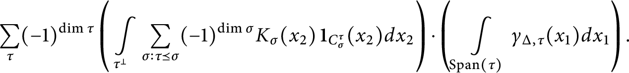 $$ \begin{align*}\sum_{\tau} (-1)^{\dim \tau} \left( \, \int\limits_{\tau^\perp} \sum_{\sigma: \tau \preceq \sigma} (-1)^{\dim \sigma} K_\sigma(x_2)\, {\textbf 1}_{C_{\sigma}^{\tau}}(x_2) dx_2 \right) \cdot \left( \, \int\limits_{\operatorname{Span}(\tau)} \gamma_{\Delta, \tau}(x_1) dx_1 \right). \end{align*} $$
Here, $x=x_1 + x_2$
where
$x=x_1 + x_2$
where $x_1 \in \operatorname {Span}(\tau )$
and
$x_1 \in \operatorname {Span}(\tau )$
and $x_2 \in \tau ^\perp $
, and
$x_2 \in \tau ^\perp $
, and $dx_1$
and
$dx_1$
and $dx_2$
are the Lebesgue measures on
$dx_2$
are the Lebesgue measures on $\operatorname {Span}(\tau )$
and
$\operatorname {Span}(\tau )$
and $\tau ^\perp $
, respectively, so that
$\tau ^\perp $
, respectively, so that $dx=dx_1 dx_2$
. By Theorem 2.1 and Remark 2.9, we know that
$dx=dx_1 dx_2$
. By Theorem 2.1 and Remark 2.9, we know that
 $$ \begin{align*} \operatorname{vol}(\Gamma_{\Delta, \tau}) = \int\limits_{\operatorname{Span}(\tau)} \gamma_{\Delta, \tau}(x_1) \, dx_1 \end{align*} $$
is a polynomial in the support numbers of $\Gamma _{\Delta , \tau }$
of degree
$\Gamma _{\Delta , \tau }$
of degree $\dim \tau $
. By definition (see (4.1)), these support numbers either correspond to the
$\dim \tau $
. By definition (see (4.1)), these support numbers either correspond to the $b_i$
in which case they are
$b_i$
in which case they are $0$
, or they correspond to the
$0$
, or they correspond to the $w_i$
in which case they are equal to the
$w_i$
in which case they are equal to the $a_i$
, the corresponding support numbers of
$a_i$
, the corresponding support numbers of $\Delta $
. It follows that
$\Delta $
. It follows that $\operatorname {vol}(\Gamma _{\Delta , \tau })$
is a polynomial in the support numbers of
$\operatorname {vol}(\Gamma _{\Delta , \tau })$
is a polynomial in the support numbers of $\Delta $
of degree
$\Delta $
of degree $\dim \tau $
. Recall that the normal fan of the face of
$\dim \tau $
. Recall that the normal fan of the face of $\Delta $
corresponding to
$\Delta $
corresponding to $\tau $
is the fan
$\tau $
is the fan $\Sigma / \tau $
consisting of all the images of the cones
$\Sigma / \tau $
consisting of all the images of the cones $\sigma \succeq \tau $
in the quotient vector space
$\sigma \succeq \tau $
in the quotient vector space $V / \operatorname {Span}(\tau ) \cong \tau ^\perp $
. One then observes that
$V / \operatorname {Span}(\tau ) \cong \tau ^\perp $
. One then observes that $\int \limits _{\tau ^\perp } \sum \limits _{\sigma : \tau \preceq \sigma } (-1)^{\dim \sigma } K_\sigma (x)\, {\textbf 1}_{C_{\sigma }^{\tau }}(x) \, dx_2$
is exactly
$\int \limits _{\tau ^\perp } \sum \limits _{\sigma : \tau \preceq \sigma } (-1)^{\dim \sigma } K_\sigma (x)\, {\textbf 1}_{C_{\sigma }^{\tau }}(x) \, dx_2$
is exactly $J_{\Sigma /\tau }(0)$
. In summary,
$J_{\Sigma /\tau }(0)$
. In summary,
 $$ \begin{align*} J_{\Sigma}(\Delta) = \sum_{\tau \in \Sigma} (-1)^{\dim \tau} J_{\Sigma/\tau}(0) \operatorname{vol}(\Gamma_{\Delta, \tau}). \end{align*} $$
This shows that $J_{\Sigma }(\Delta )$
is a linear combination of the polynomials
$J_{\Sigma }(\Delta )$
is a linear combination of the polynomials $\operatorname {vol}(\Gamma _{\Delta , \tau })$
and hence is a polynomial itself. It remains to show that
$\operatorname {vol}(\Gamma _{\Delta , \tau })$
and hence is a polynomial itself. It remains to show that $J_{\Sigma /\tau }(0)$
is convergent. But this is the content of Lemma 3.7, and the proof is finished.▪
$J_{\Sigma /\tau }(0)$
is convergent. But this is the content of Lemma 3.7, and the proof is finished.▪
Proof of Theorem 4.2
In the proof of Theorem 4.1, replace any integral $\int \limits _A f(x)dx$
with a sum
$\int \limits _A f(x)dx$
with a sum $\sum \limits _{m \in A \cap M} f(m)$
. In particular, replace
$\sum \limits _{m \in A \cap M} f(m)$
. In particular, replace $\operatorname {vol}$
with the number of lattice points. For
$\operatorname {vol}$
with the number of lattice points. For $\tau \in \Sigma $
, let
$\tau \in \Sigma $
, let $M_1 = \operatorname {Span}(\tau ) \cap M$
and
$M_1 = \operatorname {Span}(\tau ) \cap M$
and $M_2 = \tau ^\perp \cap M$
. Note that it is possible that
$M_2 = \tau ^\perp \cap M$
. Note that it is possible that $M_1 + M_2 \neq M$
. Nevertheless,
$M_1 + M_2 \neq M$
. Nevertheless, $M_1+M_2$
is a subgroup of finite index in M. Let
$M_1+M_2$
is a subgroup of finite index in M. Let $M' \subset M$
be a system of coset representatives for
$M' \subset M$
be a system of coset representatives for $M/ (M_1+M_2)$
. Then every
$M/ (M_1+M_2)$
. Then every $m \in M$
can be uniquely written as
$m \in M$
can be uniquely written as $m'+m_1+m_2$
where
$m'+m_1+m_2$
where $m' \in M'$
and
$m' \in M'$
and $m_i \in M_i$
. Then, similar to the proof of Theorem 4.1, we write
$m_i \in M_i$
. Then, similar to the proof of Theorem 4.1, we write
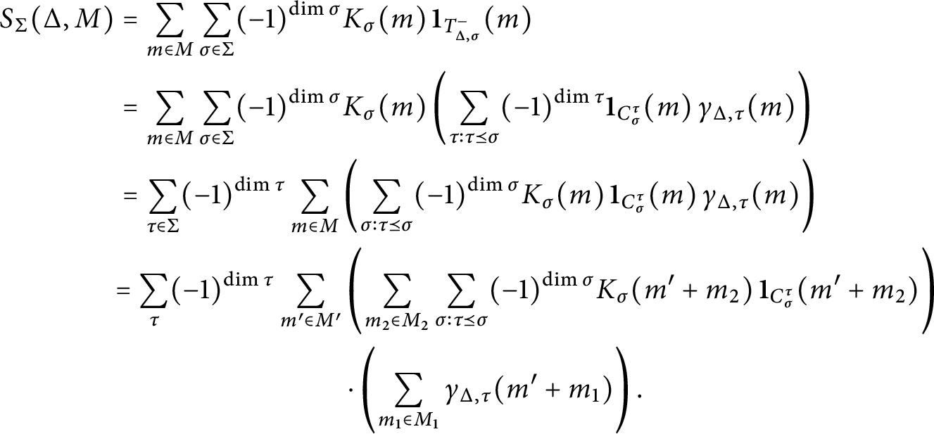 $$ \begin{align*} S_{\Sigma}(\Delta, M) &= \sum_{m \in M} \sum_{\sigma \in \Sigma} (-1)^{\dim \sigma} K_\sigma(m) \, {\textbf 1}_{T^-_{\Delta, \sigma}}(m)\\ &= \sum_{m \in M} \sum_{\sigma \in \Sigma} (-1)^{\dim \sigma} K_\sigma(m) \left(\sum_{\tau: \tau \preceq \sigma} (-1)^{\dim \tau} {\textbf 1}_{C_{\sigma}^{\tau}}(m) \, \gamma_{\Delta, \tau}(m)\right)\\ &= \sum_{\tau \in \Sigma} (-1)^{\dim \tau} \sum_{m \in M} \left(\sum_{\sigma: \tau \preceq \sigma} (-1)^{\dim \sigma} K_\sigma(m)\, {\textbf 1}_{C_{\sigma}^{\tau}}(m)\, \gamma_{\Delta, \tau}(m)\right) \nonumber \\ &\begin{aligned} =\sum_{\tau} (-1)^{\dim \tau} \sum_{m' \in M'} &\left( \sum_{m_2 \in M_2} \sum_{\sigma: \tau \preceq \sigma} (-1)^{\dim \sigma} K_\sigma(m'+m_2)\, {\textbf 1}_{C_{\sigma}^{\tau}}(m'+m_2) \right) \\ &\cdot \left( \sum_{m_1 \in M_1} \gamma_{\Delta, \tau}(m'+m_1) \right). \end{aligned} \end{align*} $$
One shows that, for fixed $m' \in M'$
, the quantity
$m' \in M'$
, the quantity $\sum \limits _{m_2 \in M_2} \sum \limits _{\sigma : \tau \preceq \sigma } (-1)^{\dim \sigma } K_\sigma (m'+m_2)$
is equal to
$\sum \limits _{m_2 \in M_2} \sum \limits _{\sigma : \tau \preceq \sigma } (-1)^{\dim \sigma } K_\sigma (m'+m_2)$
is equal to $S_{\Sigma /\tau }(0)$
with respect to the functions
$S_{\Sigma /\tau }(0)$
with respect to the functions $K_\sigma (m'+x)$
(instead of
$K_\sigma (m'+x)$
(instead of $K_\sigma (x)$
). By the discrete version of Lemma 3.7, we know that
$K_\sigma (x)$
). By the discrete version of Lemma 3.7, we know that $S_{\Sigma /\tau }(0)$
is convergent. Let us see that the other term
$S_{\Sigma /\tau }(0)$
is convergent. Let us see that the other term $\sum \limits _{m_1 \in M_1} \gamma _{\Delta , \tau }(m'+m_1)$
depends polynomially on
$\sum \limits _{m_1 \in M_1} \gamma _{\Delta , \tau }(m'+m_1)$
depends polynomially on $\Delta $
. Let
$\Delta $
. Let $\pi : V \to \operatorname {Span}(\tau )$
be the orthogonal projection. Since
$\pi : V \to \operatorname {Span}(\tau )$
be the orthogonal projection. Since $\gamma _{\Delta , \tau }$
is invariant in the
$\gamma _{\Delta , \tau }$
is invariant in the $\tau ^\perp $
direction, we have
$\tau ^\perp $
direction, we have $\gamma _{\Delta , \tau }(m'+m_1) = \gamma _{\Delta , \tau }(\pi (m')+m_1)$
. Now, the polynomiality of
$\gamma _{\Delta , \tau }(m'+m_1) = \gamma _{\Delta , \tau }(\pi (m')+m_1)$
. Now, the polynomiality of $\sum \limits _{m_1 \in M} \gamma _{\Delta , \tau }(\pi (m')+m_1)$
follows from Remark 2.9 (see also Theorem 2.3 and Remark 2.4). Thus,
$\sum \limits _{m_1 \in M} \gamma _{\Delta , \tau }(\pi (m')+m_1)$
follows from Remark 2.9 (see also Theorem 2.3 and Remark 2.4). Thus, $S_{\Sigma }(\Delta , M)$
is a finite sum (over
$S_{\Sigma }(\Delta , M)$
is a finite sum (over $m' \in M'$
) of polynomials and hence a polynomial itself. This finishes the proof.▪
$m' \in M'$
) of polynomials and hence a polynomial itself. This finishes the proof.▪
5 Toric varieties
5.1 Background on toric varieties
In this section, we review some basic facts about toric varieties. Common references on toric varieties are [Reference Cox, Little and SchenckCLS11, Reference FultonFu93]. Let $T = T_N \cong ({\mathbb C}^*)^n$
be an algebraic torus of dimension n over
$T = T_N \cong ({\mathbb C}^*)^n$
be an algebraic torus of dimension n over ${\mathbb C}$
, with character lattice
${\mathbb C}$
, with character lattice $M \cong {\mathbb Z}^n$
and cocharacter lattice
$M \cong {\mathbb Z}^n$
and cocharacter lattice $N \cong {\mathbb Z}^n$
. We denote the corresponding vector spaces
$N \cong {\mathbb Z}^n$
. We denote the corresponding vector spaces $N \otimes _{\mathbb Z} {\mathbb R}$
and
$N \otimes _{\mathbb Z} {\mathbb R}$
and $M \otimes _{\mathbb Z} {\mathbb R}$
by
$M \otimes _{\mathbb Z} {\mathbb R}$
by $N_{\mathbb R}$
and
$N_{\mathbb R}$
and $M_{\mathbb R}$
, respectively. For
$M_{\mathbb R}$
, respectively. For $m \in M$
, we denote the corresponding character/irreducible representation by
$m \in M$
, we denote the corresponding character/irreducible representation by $\chi _m: T \to {\mathbb C}^*$
.
$\chi _m: T \to {\mathbb C}^*$
.
Let $\sigma \subset N_{\mathbb R}$
be a rational strongly convex polyhedral cone. Recall that
$\sigma \subset N_{\mathbb R}$
be a rational strongly convex polyhedral cone. Recall that $\sigma $
is rational if it is generated as a cone by vectors from N. To
$\sigma $
is rational if it is generated as a cone by vectors from N. To $\sigma $
, one associates an affine toric variety
$\sigma $
, one associates an affine toric variety $U_\sigma $
defined by
$U_\sigma $
defined by
 $$ \begin{align*} U_\sigma = \operatorname{Spec}({\mathbb C}[\sigma^\vee \cap M]. \end{align*} $$
Here, ${\mathbb C}[\sigma ^\vee \cap M]$
is the semigroup algebra of the semigroup of all lattice points in the dual cone
${\mathbb C}[\sigma ^\vee \cap M]$
is the semigroup algebra of the semigroup of all lattice points in the dual cone $\sigma ^\vee $
. If
$\sigma ^\vee $
. If $\tau \preceq \sigma $
, then we have natural inclusion
$\tau \preceq \sigma $
, then we have natural inclusion $U_\tau \hookrightarrow U_\sigma $
. The variety
$U_\tau \hookrightarrow U_\sigma $
. The variety $U_0$
associated with the origin is just the algebraic torus T itself. The M-grading on the algebra
$U_0$
associated with the origin is just the algebraic torus T itself. The M-grading on the algebra ${\mathbb C}[\sigma ^\vee \cap M]$
induces a T-action on the variety
${\mathbb C}[\sigma ^\vee \cap M]$
induces a T-action on the variety $U_\sigma $
with open orbit
$U_\sigma $
with open orbit $U_0$
.
$U_0$
.
Recall that a fan $\Sigma $
in
$\Sigma $
in $N_{\mathbb R}$
is rational if all the cones in
$N_{\mathbb R}$
is rational if all the cones in $\Sigma $
are generated by vectors in N. Let
$\Sigma $
are generated by vectors in N. Let $X_{\Sigma }$
be the toric variety corresponding to a complete rational fan
$X_{\Sigma }$
be the toric variety corresponding to a complete rational fan $\Sigma $
(see [Reference Cox, Little and SchenckCLS11, Chapter 3] for more details). The (abstract) variety
$\Sigma $
(see [Reference Cox, Little and SchenckCLS11, Chapter 3] for more details). The (abstract) variety $X_{\Sigma }$
is obtained by gluing all the affine toric varieties
$X_{\Sigma }$
is obtained by gluing all the affine toric varieties $U_\sigma $
,
$U_\sigma $
, $\sigma \in \Sigma $
, with respect to inclusion maps
$\sigma \in \Sigma $
, with respect to inclusion maps $U_\tau \hookrightarrow U_\sigma $
and
$U_\tau \hookrightarrow U_\sigma $
and $\tau \preceq \sigma $
.
$\tau \preceq \sigma $
.
There is an inclusion-reversing correspondence between the cones in $\Sigma $
and the T-orbits in
$\Sigma $
and the T-orbits in $X_{\Sigma }$
. For
$X_{\Sigma }$
. For $\sigma \in \Sigma $
, let the corresponding T-orbit be
$\sigma \in \Sigma $
, let the corresponding T-orbit be $O_\sigma $
.
$O_\sigma $
.
For a ray $\rho \in \Sigma (1)$
, we denote the corresponding T-orbit closure
$\rho \in \Sigma (1)$
, we denote the corresponding T-orbit closure $\overline {O}_\rho $
by
$\overline {O}_\rho $
by $D_\rho $
. The
$D_\rho $
. The $D_\rho $
for
$D_\rho $
for $\rho \in \Sigma (1)$
are T-invariant prime divisors on
$\rho \in \Sigma (1)$
are T-invariant prime divisors on $X_{\Sigma }$
. For each ray
$X_{\Sigma }$
. For each ray $\rho \in \Sigma (1)$
, let
$\rho \in \Sigma (1)$
, let $v_\rho \in N$
be the primitive vector along
$v_\rho \in N$
be the primitive vector along $\rho $
, i.e., shortest lattice vector on
$\rho $
, i.e., shortest lattice vector on $\rho $
. Let
$\rho $
. Let $\xi \in \sigma \cap N$
be a cocharacter. One knows that for
$\xi \in \sigma \cap N$
be a cocharacter. One knows that for $x \in U_0$
,
$x \in U_0$
, $\lim _{t \to 0} \xi (t) \cdot x$
exists and is a point in the orbit
$\lim _{t \to 0} \xi (t) \cdot x$
exists and is a point in the orbit $O_\sigma $
.
$O_\sigma $
.
Let us assume that $X_{\Sigma }$
is a projective variety. This is equivalent to the set
$X_{\Sigma }$
is a projective variety. This is equivalent to the set $\mathcal {P}(\Sigma )$
, of polytopes with normal fan
$\mathcal {P}(\Sigma )$
, of polytopes with normal fan $\Sigma $
, being nonempty. Let
$\Sigma $
, being nonempty. Let $\Delta \subset M_{\mathbb R}$
be a lattice polytope with normal fan
$\Delta \subset M_{\mathbb R}$
be a lattice polytope with normal fan $\Sigma $
. The faces of
$\Sigma $
. The faces of $\Delta $
are in one-to-one correspondence with cones in
$\Delta $
are in one-to-one correspondence with cones in $\Sigma $
. For
$\Sigma $
. For $\sigma \in \Sigma $
, let
$\sigma \in \Sigma $
, let $Q_\sigma $
be the corresponding face of
$Q_\sigma $
be the corresponding face of $\Delta $
. We note that
$\Delta $
. We note that $\dim Q_\sigma = \operatorname {codim} \sigma $
. The polytope
$\dim Q_\sigma = \operatorname {codim} \sigma $
. The polytope $\Delta $
can be represented as
$\Delta $
can be represented as
 $$ \begin{align} \Delta = \{ x \in M_{\mathbb R} : \langle x, v_\rho \rangle \leqslant -a_\rho, \forall \rho \in \Sigma(1) \}, \end{align} $$
where the $a_\rho $
are the support numbers of
$a_\rho $
are the support numbers of $\Delta $
(see Section 2). Recall that for
$\Delta $
(see Section 2). Recall that for $\sigma \in \Sigma $
, we let
$\sigma \in \Sigma $
, we let $T^+_{\Delta , \sigma }$
(resp.
$T^+_{\Delta , \sigma }$
(resp. $T^-_{\Delta , \sigma }$
) be the inward-looking (resp. outward-looking) tangent cone of the corresponding face
$T^-_{\Delta , \sigma }$
) be the inward-looking (resp. outward-looking) tangent cone of the corresponding face $Q_\sigma $
in
$Q_\sigma $
in $\Delta $
(see equations (2.2) and (2.3)).
$\Delta $
(see equations (2.2) and (2.3)).
To $\Delta $
, one associates a T-invariant (Cartier) divisor
$\Delta $
, one associates a T-invariant (Cartier) divisor
 $$ \begin{align*} D_\Delta = \sum_{\rho \in \Sigma(1)} -a_\rho D_\rho. \end{align*} $$
It can be shown that $D_\Delta $
is an ample divisor. We denote the corresponding line bundle on
$D_\Delta $
is an ample divisor. We denote the corresponding line bundle on $X_{\Sigma }$
by
$X_{\Sigma }$
by $\mathcal {L}_\Delta $
. Since
$\mathcal {L}_\Delta $
. Since $D_\Delta $
is T-invariant, the line bundle
$D_\Delta $
is T-invariant, the line bundle $\mathcal {L}_\Delta $
comes with a natural T-linearization. The divisor
$\mathcal {L}_\Delta $
comes with a natural T-linearization. The divisor $D_\Delta $
defines a sheaf of rational functions
$D_\Delta $
defines a sheaf of rational functions ${\mathcal O}(D_\Delta )$
by
${\mathcal O}(D_\Delta )$
by
 $$ \begin{align} H^0(U, {\mathcal O}(D_\Delta)) &= \{ f \in {\mathbb C}(X_{\Sigma}) : (f) + D_\Delta> 0 \text{ on } U \} \subset {\mathbb C}[U_0], \end{align} $$
 $$ \begin{align} &= \{ f \in {\mathbb C}(X_{\Sigma}) : \operatorname{ord}_{D_\rho}(f) \geqslant a_\rho,~ \forall \rho \in \Sigma(1) \text{ such that } D_\rho \cap U \neq \emptyset\}. \end{align} $$
In particular, for an open affine chart $U_\sigma $
, the subspace
$U_\sigma $
, the subspace $H^0(U_\sigma , {\mathcal O}(D_\Delta ))$
is T-invariant and hence decomposes into one-dimensional T-modules. Let
$H^0(U_\sigma , {\mathcal O}(D_\Delta ))$
is T-invariant and hence decomposes into one-dimensional T-modules. Let $m \in M$
. One verifies that for any ray
$m \in M$
. One verifies that for any ray $\rho \in \Sigma (1)$
, the order of zero/pole of the character
$\rho \in \Sigma (1)$
, the order of zero/pole of the character $\chi _m$
, regarded as a rational function on
$\chi _m$
, regarded as a rational function on $U_0 \cong T$
, along the divisor
$U_0 \cong T$
, along the divisor $D_\rho $
is given by
$D_\rho $
is given by
 $$ \begin{align*} \operatorname{ord}_{D_\rho}(\chi_m) = - \langle m, v_\rho \rangle. \end{align*} $$
It follows that, for any $\sigma \in \Sigma $
, the irreducible representation
$\sigma \in \Sigma $
, the irreducible representation $\chi _m$
appears in
$\chi _m$
appears in $H^0(U_\sigma , {\mathcal O}(D_\Delta ))$
if and only if
$H^0(U_\sigma , {\mathcal O}(D_\Delta ))$
if and only if $\langle m, v_\rho \rangle \leqslant -a_\rho $
, for all
$\langle m, v_\rho \rangle \leqslant -a_\rho $
, for all $\rho \in \sigma (1)$
. Since
$\rho \in \sigma (1)$
. Since ${\mathbb C}[U_0]$
, the coordinate ring of the algebraic torus, is multiplicity-free as a T-module, it follows that
${\mathbb C}[U_0]$
, the coordinate ring of the algebraic torus, is multiplicity-free as a T-module, it follows that $H^0(U_\sigma , {\mathcal O}(D_\Delta ))$
is also multiplicity-free. Thus, the T-module
$H^0(U_\sigma , {\mathcal O}(D_\Delta ))$
is also multiplicity-free. Thus, the T-module $H^0(U_\sigma , {\mathcal O}(D_\Delta ))$
decomposes into one-dimensional irreducible representation as
$H^0(U_\sigma , {\mathcal O}(D_\Delta ))$
decomposes into one-dimensional irreducible representation as
 $$ \begin{align} H^0(U_\sigma, {\mathcal O}(D_\Delta)) = \bigoplus_{m \in T^+_{\Delta, \sigma} \cap M} \chi_m, \end{align} $$
where as before $T^+_{\Delta , \sigma }$
denotes the inward-looking tangent cone of
$T^+_{\Delta , \sigma }$
denotes the inward-looking tangent cone of $\Delta $
at the face corresponding to
$\Delta $
at the face corresponding to $\sigma $
. Similarly,
$\sigma $
. Similarly, $\chi _m$
appears in the space of global sections
$\chi _m$
appears in the space of global sections $H^0(X_{\Sigma }, {\mathcal O}(D_\Delta ))$
if and only if
$H^0(X_{\Sigma }, {\mathcal O}(D_\Delta ))$
if and only if $\langle m, v_\rho \rangle \leqslant -a_\rho $
, for all
$\langle m, v_\rho \rangle \leqslant -a_\rho $
, for all $\rho \in \Sigma (1)$
, and we have
$\rho \in \Sigma (1)$
, and we have
 $$ \begin{align} H^0(X_{\Sigma}, {\mathcal O}(D_\Delta)) = \bigoplus_{m \in \Delta \cap M} \chi_m. \end{align} $$
This implies that $\dim (H^0(X_{\Sigma }, {\mathcal O}(D_\Delta )) = |\Delta \cap M|$
, the number of lattice points in M.
$\dim (H^0(X_{\Sigma }, {\mathcal O}(D_\Delta )) = |\Delta \cap M|$
, the number of lattice points in M.
5.2 Brianchon–Gram theorem and equivariant Euler characteristic
Let ${\mathcal F}$
be a T-linearized sheaf (of rational functions) on
${\mathcal F}$
be a T-linearized sheaf (of rational functions) on $X_{\Sigma }$
, that is, for any T-invariant open set U, the space of sections
$X_{\Sigma }$
, that is, for any T-invariant open set U, the space of sections $H^0(U, {\mathcal F})$
is a T-module and the restriction maps are T-equivariant. For
$H^0(U, {\mathcal F})$
is a T-module and the restriction maps are T-equivariant. For $m \in M$
and V a T-module, let
$m \in M$
and V a T-module, let $V_m$
denote the m-isotypic component of V. By the equivariant Euler characteristic of
$V_m$
denote the m-isotypic component of V. By the equivariant Euler characteristic of ${\mathcal F}$
, we mean the function
${\mathcal F}$
, we mean the function $\chi _T(X_{\Sigma }, {\mathcal F}): M \to {\mathbb Z}_{\geq 0}$
given by
$\chi _T(X_{\Sigma }, {\mathcal F}): M \to {\mathbb Z}_{\geq 0}$
given by
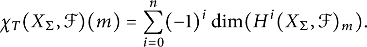 $$ \begin{align*} \chi_T(X_{\Sigma}, {\mathcal F})(m) = \sum_{i=0}^n (-1)^i \dim(H^i(X_{\Sigma}, {\mathcal F})_m). \end{align*} $$
Let us compute the equivariant Euler characteristic of the T-linearized sheaf ${\mathcal O}(D_\Delta )$
. As explained above, for each cone
${\mathcal O}(D_\Delta )$
. As explained above, for each cone $\sigma \in \Sigma $
, the T-module
$\sigma \in \Sigma $
, the T-module $H^0(U_\sigma , {\mathcal O}(D_\Delta ))$
decomposes as
$H^0(U_\sigma , {\mathcal O}(D_\Delta ))$
decomposes as
 $$ \begin{align*} H^0(U_\sigma, {\mathcal O}(D_\Delta)) = \bigoplus_{m \in T^+_{\Delta, \sigma} \cap M} \chi_m. \end{align*} $$
Recall that $T^+_{\Delta , \sigma }$
denotes the inward tangent cone of
$T^+_{\Delta , \sigma }$
denotes the inward tangent cone of $\Delta $
at the face corresponding to
$\Delta $
at the face corresponding to $\sigma $
(see Section 2.2).
$\sigma $
(see Section 2.2).
From above, it follows that the equivariant Euler characteristic $\chi _T(X_{\Sigma }, {\mathcal O}(D_\Delta ))$
, computed using Čech cohomology, can be written as:
$\chi _T(X_{\Sigma }, {\mathcal O}(D_\Delta ))$
, computed using Čech cohomology, can be written as:
 $$ \begin{align} \chi_T(X_{\Sigma}, {\mathcal O}(D_\Delta)) = \sum_{\sigma \in \Sigma} (-1)^{\dim(Q_\sigma)} {\textbf 1}_{T^+_{\Delta, \sigma} \cap M}, \end{align} $$
where as usual ${\textbf 1}_A$
denotes the characteristic function of a set A.
${\textbf 1}_A$
denotes the characteristic function of a set A.
One knows that ${\mathcal O}(D_\Delta )$
is ample and hence
${\mathcal O}(D_\Delta )$
is ample and hence $H^i(X_{\Sigma }, {\mathcal O}(D_\Delta )) = 0$
for
$H^i(X_{\Sigma }, {\mathcal O}(D_\Delta )) = 0$
for $i> 0$
. Thus, we also obtain
$i> 0$
. Thus, we also obtain
 $$ \begin{align} \chi_T(X_{\Sigma}, {\mathcal O}(D_\Delta))(m) = \dim(H^0(X_{\Sigma}, {\mathcal O}(D_\Delta))_m), \quad \forall m \in M. \end{align} $$
And hence, from (5.5), we have
 $$ \begin{align} \chi_T(X_{\Sigma}, {\mathcal O}(D_\Delta)) = {\textbf 1}_{\Delta \cap M}. \end{align} $$
Comparing with (5.6), one recovers the Brianchon–Gram theorem (Theorem 2.6).
The alternative version of the Brianchon–Gram theorem using outward face cones (Theorem 2.7) can also be obtained in a similar fashion. Let $\Delta '$
be the polytope with support numbers
$\Delta '$
be the polytope with support numbers $a_\rho + 1$
and
$a_\rho + 1$
and $D' = D_{\Delta '} = \sum \limits _{\rho \in \Sigma (1)} -(a_\rho + 1) D_\rho $
the corresponding Cartier divisor. Note that
$D' = D_{\Delta '} = \sum \limits _{\rho \in \Sigma (1)} -(a_\rho + 1) D_\rho $
the corresponding Cartier divisor. Note that $\langle x, v_\rho \rangle \leqslant -(a_\rho + 1)$
if and only
$\langle x, v_\rho \rangle \leqslant -(a_\rho + 1)$
if and only $\langle -x, v_\rho \rangle>a_\rho $
. Thus, for all
$\langle -x, v_\rho \rangle>a_\rho $
. Thus, for all $m \in M$
, we have
$m \in M$
, we have
 $$ \begin{align} \chi_T(X_{\Sigma}, {\mathcal O}(-D'))(m) = \sum_{\sigma \in \Sigma} (-1)^{n - \dim \sigma} {\textbf 1}_{T^-_{\Delta, \sigma} \cap M}(-m) \end{align} $$
(recall (2.3) for defining inequalities of outward tangent cone $T^-_{\Delta , \sigma }$
). On the other hand, the Khovanskii–Pukhlikov formula for inverse of the polytope
$T^-_{\Delta , \sigma }$
). On the other hand, the Khovanskii–Pukhlikov formula for inverse of the polytope $\Delta $
with respect to the convolution
$\Delta $
with respect to the convolution $*$
(see Section 2.6) tells us that:
$*$
(see Section 2.6) tells us that:
 $$ \begin{align} \chi_T(X_{\Sigma}, {\mathcal O}(-D'))(m) = (-1)^n \chi_T(X_{\Sigma}, {\mathcal O}(D_\Delta))(-m) = (-1)^n {\textbf 1}_{\Delta \cap M}(-m). \end{align} $$
Putting together (5.9) and (5.10), we obtain
 $$ \begin{align*} (-1)^n {\textbf 1}_{\Delta \cap M} = \sum_{\sigma \in \Sigma} (-1)^{n - \dim \sigma} {\textbf 1}_{T^-_{\Delta, \sigma} \cap M}, \end{align*} $$
which immediately implies Theorem 2.7.
Remark 5.1 (A symplectic interpretation of the Brianchon–Gram theorem)
We can also give a symplectic geometric interpretation of the Brianchon–Gram theorem, namely as an identity between Liouville measures. Let X be a symplectic manifold with a Hamiltonian $S^1$
-action with moment map
$S^1$
-action with moment map $\mu : X \to {\mathbb R}$
. This means that the Hamiltonian vector field of
$\mu : X \to {\mathbb R}$
. This means that the Hamiltonian vector field of $\mu $
generates the
$\mu $
generates the $S^1$
-action. Let
$S^1$
-action. Let $\epsilon $
be a regular value of the moment map
$\epsilon $
be a regular value of the moment map $\mu $
. Then
$\mu $
. Then $\mu ^{-1}([\epsilon , \infty ))$
is a manifold with boundary. The symplectic cut
$\mu ^{-1}([\epsilon , \infty ))$
is a manifold with boundary. The symplectic cut $\overline {X}_{\mu \geq \epsilon }$
is the manifold obtained by collapsing each
$\overline {X}_{\mu \geq \epsilon }$
is the manifold obtained by collapsing each $S^1$
-orbit in the boundary
$S^1$
-orbit in the boundary $\mu ^{-1}(\epsilon )$
to a point.
$\mu ^{-1}(\epsilon )$
to a point.
We can decompose $T = ({\mathbb C}^*)^n$
as
$T = ({\mathbb C}^*)^n$
as $T = (S^1)^n \times {\mathbb R}_{>0}^n$
. Equip T with the standard symplectic form from
$T = (S^1)^n \times {\mathbb R}_{>0}^n$
. Equip T with the standard symplectic form from ${\mathbb C}^n$
. Each ray
${\mathbb C}^n$
. Each ray $\rho \in \Sigma (1)$
defines a Hamiltonian function
$\rho \in \Sigma (1)$
defines a Hamiltonian function $\mu _\rho : U_0 \to {\mathbb R}$
on
$\mu _\rho : U_0 \to {\mathbb R}$
on $U_0 \cong T$
by
$U_0 \cong T$
by
 $$ \begin{align*}\mu_\rho(x) = |x|^{v_\rho} := |x_1|^{r_1} \cdots |x_n|^{r_n},\end{align*} $$
where $x=(x_1, \ldots , x_n)$
and
$x=(x_1, \ldots , x_n)$
and $v_\rho = (r_1, \ldots , r_n)$
. One verifies that the Hamiltonian vector field of
$v_\rho = (r_1, \ldots , r_n)$
. One verifies that the Hamiltonian vector field of $\mu _\rho $
generates the
$\mu _\rho $
generates the ${\mathbb C}^*$
-action on T corresponding to the cocharacter
${\mathbb C}^*$
-action on T corresponding to the cocharacter $v_\rho \in N$
. Let
$v_\rho \in N$
. Let $\Sigma $
be a smooth fan, let
$\Sigma $
be a smooth fan, let $\Delta $
be a rational polytope with normal fan
$\Delta $
be a rational polytope with normal fan $\Sigma $
, and let
$\Sigma $
, and let $a_\rho $
,
$a_\rho $
, $\rho \in \Sigma (1)$
, be its support numbers. Starting with
$\rho \in \Sigma (1)$
, be its support numbers. Starting with $({\mathbb C}^*)^n$
, doing repeated symplectic cuts with respect to the
$({\mathbb C}^*)^n$
, doing repeated symplectic cuts with respect to the $\mu =\mu _\rho $
and
$\mu =\mu _\rho $
and $\epsilon =a_\rho $
,
$\epsilon =a_\rho $
, $\rho \in \Sigma (1)$
, one arrives at the toric variety
$\rho \in \Sigma (1)$
, one arrives at the toric variety $X_{\Sigma }$
. One can show that the open affine chart
$X_{\Sigma }$
. One can show that the open affine chart $U_\sigma $
is the symplectic manifold obtained by symplectic cuts using rays of
$U_\sigma $
is the symplectic manifold obtained by symplectic cuts using rays of $\sigma $
. Moreover, the image of the moment map of
$\sigma $
. Moreover, the image of the moment map of $U_\sigma $
is the inward tangent cone
$U_\sigma $
is the inward tangent cone $T^+_{\Delta , \sigma }$
.
$T^+_{\Delta , \sigma }$
.
The Brianchon–Gram equality (2.5) can be thought of as an equality involving pushforwards (to $N_{\mathbb R} = {\mathbb R}^n$
) of Liouville measures on all the symplectic manifolds
$N_{\mathbb R} = {\mathbb R}^n$
) of Liouville measures on all the symplectic manifolds $U_{\sigma }$
and
$U_{\sigma }$
and $X_{\Sigma }$
.
$X_{\Sigma }$
.
5.3 Positive part of a toric variety and logarithm map
As before, let $X_{\Sigma }$
be the toric variety associated with a rational fan
$X_{\Sigma }$
be the toric variety associated with a rational fan $\Sigma $
in
$\Sigma $
in $N_{\mathbb R}$
. Take
$N_{\mathbb R}$
. Take $\sigma \in \Sigma $
. By definition, the set
$\sigma \in \Sigma $
. By definition, the set $U_\sigma ({\mathbb C})$
of points of
$U_\sigma ({\mathbb C})$
of points of $U_\sigma $
defined over
$U_\sigma $
defined over ${\mathbb C}$
is the set of maximal ideals of the semigroup algebra
${\mathbb C}$
is the set of maximal ideals of the semigroup algebra ${\mathbb C}[\sigma ^\vee \cap M]$
. This set then can be identified with
${\mathbb C}[\sigma ^\vee \cap M]$
. This set then can be identified with $\operatorname {Hom}(\sigma ^\vee \cap M, {\mathbb C})$
, where
$\operatorname {Hom}(\sigma ^\vee \cap M, {\mathbb C})$
, where $\operatorname {Hom}$
denotes the semigroup homomorphisms. This observation enables us to construct
$\operatorname {Hom}$
denotes the semigroup homomorphisms. This observation enables us to construct $X_{\Sigma }^+$
, the points of
$X_{\Sigma }^+$
, the points of $X_{\Sigma }$
over the semigroup
$X_{\Sigma }$
over the semigroup ${\mathbb R}_{\geq 0}$
(see [Reference FultonFu93, Section 4.1]). We think of
${\mathbb R}_{\geq 0}$
(see [Reference FultonFu93, Section 4.1]). We think of $X_{\Sigma }^+$
as the “positive” part of
$X_{\Sigma }^+$
as the “positive” part of $X_{\Sigma }({\mathbb C})$
. It is constructed as follows. For each
$X_{\Sigma }({\mathbb C})$
. It is constructed as follows. For each $\sigma \in \Sigma $
, let
$\sigma \in \Sigma $
, let $U_\sigma ^+ = \operatorname {Hom}(\sigma ^\vee \cap M, {\mathbb R}_{\geq 0})$
. Then, as before, the
$U_\sigma ^+ = \operatorname {Hom}(\sigma ^\vee \cap M, {\mathbb R}_{\geq 0})$
. Then, as before, the $U_\sigma ^+$
glue together to give
$U_\sigma ^+$
glue together to give $X_{\Sigma }^+$
. One has natural inclusion
$X_{\Sigma }^+$
. One has natural inclusion $X_{\Sigma }^+ \hookrightarrow X_{\Sigma }({\mathbb C})$
. Moreover, the absolute value
$X_{\Sigma }^+ \hookrightarrow X_{\Sigma }({\mathbb C})$
. Moreover, the absolute value $| \cdot |: {\mathbb C} \to {\mathbb R}_{\geq 0}$
induces a retraction map
$| \cdot |: {\mathbb C} \to {\mathbb R}_{\geq 0}$
induces a retraction map $X_{\Sigma }({\mathbb C}) \to X_{\Sigma }^+$
. Let
$X_{\Sigma }({\mathbb C}) \to X_{\Sigma }^+$
. Let $T_K = (S^1)^n$
denote the usual compact torus which is the maximal compact subgroup of T. One verifies that the retraction map induces a homeomorphism between the quotient
$T_K = (S^1)^n$
denote the usual compact torus which is the maximal compact subgroup of T. One verifies that the retraction map induces a homeomorphism between the quotient $X_{\Sigma }({\mathbb C}) / T_K$
and
$X_{\Sigma }({\mathbb C}) / T_K$
and $X_{\Sigma }^+$
.
$X_{\Sigma }^+$
.
Another way to look at $X_{\Sigma }^+$
is as follows. Consider the logarithm map
$X_{\Sigma }^+$
is as follows. Consider the logarithm map
 $$\begin{align*}\operatorname{Log}: T_N = ({\mathbb C}^*)^n \longrightarrow N_{\mathbb R} = \operatorname{Hom}(M, {\mathbb R}) \end{align*}$$
defined as follows. For $z \in T$
and
$z \in T$
and $m \in M$
, let
$m \in M$
, let
 $$ \begin{align} \operatorname{Log}(z)(m) = \log( |\chi_m(z)|). \end{align} $$
In the standard coordinates for $({\mathbb C}^*)^n$
, the logarithm map is given by
$({\mathbb C}^*)^n$
, the logarithm map is given by
 $$ \begin{align} \operatorname{Log}(z_1, \ldots, z_n) = (\log|z_1|, \ldots, \log|z_n|). \end{align} $$
For each $\sigma \in \Sigma $
, the orbit
$\sigma \in \Sigma $
, the orbit $O_\sigma $
can be identified with
$O_\sigma $
can be identified with $T / T_\sigma $
where
$T / T_\sigma $
where $T_\sigma $
is the T-stabilizer of
$T_\sigma $
is the T-stabilizer of $O_\sigma $
. Let
$O_\sigma $
. Let $N_\sigma $
denote the cocharacter lattice of
$N_\sigma $
denote the cocharacter lattice of $T_\sigma $
. It follows from the definitions that
$T_\sigma $
. It follows from the definitions that $N_\sigma \otimes {\mathbb R} = \operatorname {Span}(\sigma )$
. The logarithm map then induces a map
$N_\sigma \otimes {\mathbb R} = \operatorname {Span}(\sigma )$
. The logarithm map then induces a map $\operatorname {Log}_\sigma : T/T_\sigma \to N_{\mathbb R} / \operatorname {Span}(\sigma )$
. In the same way, that
$\operatorname {Log}_\sigma : T/T_\sigma \to N_{\mathbb R} / \operatorname {Span}(\sigma )$
. In the same way, that $X_{\Sigma }({\mathbb C})$
is a disjoint union of the tori
$X_{\Sigma }({\mathbb C})$
is a disjoint union of the tori $O_\sigma $
,
$O_\sigma $
, $\sigma \in \Sigma $
, the positive part
$\sigma \in \Sigma $
, the positive part $X_{\Sigma }^+$
, is a disjoint union of the real vector spaces
$X_{\Sigma }^+$
, is a disjoint union of the real vector spaces $N_{\mathbb R} / \operatorname {Span}(\sigma )$
,
$N_{\mathbb R} / \operatorname {Span}(\sigma )$
, $\sigma \in \Sigma $
.
$\sigma \in \Sigma $
.
Finally, $X_{\Sigma }^+$
is actually homeomorphic to a polytope (in a nonunique way). Given a polytope
$X_{\Sigma }^+$
is actually homeomorphic to a polytope (in a nonunique way). Given a polytope $\Delta $
with normal fan
$\Delta $
with normal fan $\Sigma $
, one can construct explicitly a
$\Sigma $
, one can construct explicitly a $T_K$
-invariant continuous map
$T_K$
-invariant continuous map $\mu : X_{\Sigma } \to \Delta $
such that the induced map
$\mu : X_{\Sigma } \to \Delta $
such that the induced map $\bar {\mu }: X_{\Sigma } / T_K \to \Delta $
is a homeomorphism and the following diagram is commutative (see [Reference FultonFu93, Section 4.2]).
$\bar {\mu }: X_{\Sigma } / T_K \to \Delta $
is a homeomorphism and the following diagram is commutative (see [Reference FultonFu93, Section 4.2]).
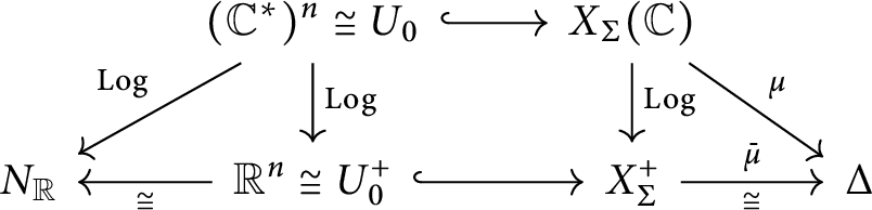
Moreover, the bottom row gives a homeomorphism between $N_{\mathbb R}$
and the interior
$N_{\mathbb R}$
and the interior $\Delta ^\circ $
of
$\Delta ^\circ $
of $\Delta $
. The map
$\Delta $
. The map $\mu $
is a special case of the notion of momentum map from the theory of Hamiltonian group actions in symplectic geometry.
$\mu $
is a special case of the notion of momentum map from the theory of Hamiltonian group actions in symplectic geometry.
6 Geometric interpretations of combinatorial truncation
We propose two geometric interpretations of our combinatorial truncation in terms of geometric notions on toric varieties. The same ideas should extend to give geometric interpretations of Arthur’s truncation and modified kernel. We expect that in this case one should replace a toric variety $X_{\Sigma }$
by Mumford’s compactification of a reductive algebraic group as in [Reference Kempf, Knudsen, Mumford and Saint-DonatKKMS73, Section IV.2].
$X_{\Sigma }$
by Mumford’s compactification of a reductive algebraic group as in [Reference Kempf, Knudsen, Mumford and Saint-DonatKKMS73, Section IV.2].
6.1 Combinatorial truncation as a complex measure on a toric variety
In this section, we propose that combinatorial truncation can be interpreted as a “truncated” complex measure on a projective toric variety, obtained from the data of prescribed measures on each torus orbit as well as choice of a polytope normal to the fan which determines certain neighborhoods of the torus orbits.
As usual, let $X_{\Sigma }$
be the toric variety associated with a (rational) fan
$X_{\Sigma }$
be the toric variety associated with a (rational) fan $\Sigma $
in
$\Sigma $
in $N_{\mathbb R}$
. Recall that the starting data of combinatorial truncation are a collection of functions
$N_{\mathbb R}$
. Recall that the starting data of combinatorial truncation are a collection of functions $\{K_\sigma : N_{\mathbb R} \to {\mathbb C}: \sigma \in \Sigma \}$
, where each
$\{K_\sigma : N_{\mathbb R} \to {\mathbb C}: \sigma \in \Sigma \}$
, where each $K_\sigma $
is invariant in the direction of
$K_\sigma $
is invariant in the direction of $\operatorname {Span}(\sigma )$
.
$\operatorname {Span}(\sigma )$
.
As before, let $T_K = (S^1)^n$
denote the compact torus in
$T_K = (S^1)^n$
denote the compact torus in $T = ({\mathbb C}^*)^n$
, which is the maximal compact subgroup of T. Suppose we are given a
$T = ({\mathbb C}^*)^n$
, which is the maximal compact subgroup of T. Suppose we are given a $T_K$
-invariant complex measure
$T_K$
-invariant complex measure $\omega _0 = f_0 d\mu _0$
on
$\omega _0 = f_0 d\mu _0$
on $U_0 = T$
where
$U_0 = T$
where $f_0$
is a continuous function on
$f_0$
is a continuous function on $U_0$
and
$U_0$
and $d\mu _0$
denotes a Haar measure on
$d\mu _0$
denotes a Haar measure on $U_0$
. Moreover, suppose, for each
$U_0$
. Moreover, suppose, for each $\{0\} \neq \sigma \in \Sigma $
, we have a
$\{0\} \neq \sigma \in \Sigma $
, we have a $T_K$
-invariant complex measure
$T_K$
-invariant complex measure $\omega _\sigma = f_\sigma d\mu _\sigma $
on the torus orbit
$\omega _\sigma = f_\sigma d\mu _\sigma $
on the torus orbit $O_\sigma $
, the T-orbit in
$O_\sigma $
, the T-orbit in $X_{\Sigma }$
associated with
$X_{\Sigma }$
associated with $\sigma $
. Here,
$\sigma $
. Here, $f_\sigma $
is a continuous function on
$f_\sigma $
is a continuous function on $O_\sigma $
, and
$O_\sigma $
, and $d\mu _\sigma $
is the Haar measure on
$d\mu _\sigma $
is the Haar measure on $O_\sigma $
induced from
$O_\sigma $
induced from $d\mu _0$
. Recall that
$d\mu _0$
. Recall that $O_\sigma \cong T / T_\sigma $
is itself isomorphic to a torus, where
$O_\sigma \cong T / T_\sigma $
is itself isomorphic to a torus, where $T_\sigma \subset T$
is the stabilizer of any point in
$T_\sigma \subset T$
is the stabilizer of any point in $O_\sigma $
. Since
$O_\sigma $
. Since $\omega _\sigma $
, and hence
$\omega _\sigma $
, and hence $f_\sigma $
, are
$f_\sigma $
, are $T_K$
-invariant, the function
$T_K$
-invariant, the function $f_\sigma $
induces a continuous function
$f_\sigma $
induces a continuous function $k_\sigma : N_{\mathbb R} / \operatorname {Span}(\sigma ) \longrightarrow {\mathbb C}$
.
$k_\sigma : N_{\mathbb R} / \operatorname {Span}(\sigma ) \longrightarrow {\mathbb C}$
.
The projection $N_{\mathbb R} \to N_{\mathbb R}/\operatorname {Span}{\sigma }$
maps the cone
$N_{\mathbb R} \to N_{\mathbb R}/\operatorname {Span}{\sigma }$
maps the cone $\sigma $
to
$\sigma $
to $\{0\}$
. This gives us an equivariant morphism
$\{0\}$
. This gives us an equivariant morphism $\pi _\sigma $
from the T-toric variety
$\pi _\sigma $
from the T-toric variety $U_\sigma $
to the
$U_\sigma $
to the $(T/T_\sigma )$
-toric variety
$(T/T_\sigma )$
-toric variety $O_\sigma $
(see [Reference Cox, Little and SchenckCLS11, Section 3.3]). We can use
$O_\sigma $
(see [Reference Cox, Little and SchenckCLS11, Section 3.3]). We can use $\pi _\sigma : U_\sigma \to O_\sigma $
to extend the measure
$\pi _\sigma : U_\sigma \to O_\sigma $
to extend the measure $\omega _\sigma $
to a measure
$\omega _\sigma $
to a measure $\Omega _\sigma $
on the affine toric chart
$\Omega _\sigma $
on the affine toric chart $U_\sigma \subset X_{\Sigma }$
(and, in particular, on the open orbit
$U_\sigma \subset X_{\Sigma }$
(and, in particular, on the open orbit $U_0 \cong T$
) by defining
$U_0 \cong T$
) by defining
 $$ \begin{align*} \Omega_\sigma = \pi_\sigma^*(\omega_\sigma). \end{align*} $$
The measure $\Omega _\sigma $
then gives a continuous function
$\Omega _\sigma $
then gives a continuous function $K_\sigma : N_{\mathbb R} \to {\mathbb C}$
which is invariant in the direction of
$K_\sigma : N_{\mathbb R} \to {\mathbb C}$
which is invariant in the direction of $\operatorname {Span}(\sigma )$
.
$\operatorname {Span}(\sigma )$
.
Now, fix an inner product $\langle \cdot , \cdot \rangle $
on
$\langle \cdot , \cdot \rangle $
on $N_{\mathbb R}$
and identify
$N_{\mathbb R}$
and identify $M_{\mathbb R}$
with
$M_{\mathbb R}$
with $N_{\mathbb R}$
via
$N_{\mathbb R}$
via $\langle \cdot , \cdot \rangle $
. As usual, take a polytope
$\langle \cdot , \cdot \rangle $
. As usual, take a polytope $\Delta \subset M_{\mathbb R} \cong N_{\mathbb R}$
with normal fan
$\Delta \subset M_{\mathbb R} \cong N_{\mathbb R}$
with normal fan $\Sigma $
. Recall that
$\Sigma $
. Recall that $\operatorname {Log}: T \to N_{\mathbb R}$
denotes the logarithm map on the torus, which extends to
$\operatorname {Log}: T \to N_{\mathbb R}$
denotes the logarithm map on the torus, which extends to $\operatorname {Log}: X_{\Sigma } \to X_{\Sigma }^+$
(see (5.11) and the diagram (5.13)). Consider the tangent cone
$\operatorname {Log}: X_{\Sigma } \to X_{\Sigma }^+$
(see (5.11) and the diagram (5.13)). Consider the tangent cone $T^-_{\Delta , \sigma }$
. We regard it as an open subset of
$T^-_{\Delta , \sigma }$
. We regard it as an open subset of $U_0^+ \cong N_{\mathbb R} \cong {\mathbb R}^n$
and hence as an open subset of
$U_0^+ \cong N_{\mathbb R} \cong {\mathbb R}^n$
and hence as an open subset of $X_{\Sigma }^+$
. We have
$X_{\Sigma }^+$
. We have
 $$ \begin{align*} U_{\Delta, \sigma} = \operatorname{Log}^{-1}(T^-_{\Delta, \sigma}). \end{align*} $$
We can also define the subset $U_{\Delta } \subset U_0$
by
$U_{\Delta } \subset U_0$
by
 $$ \begin{align*} U_{\Delta} = \operatorname{Log}^{-1}(\Delta). \end{align*} $$
We think of $\Omega _\sigma \, {\textbf 1}_{U_{\sigma , \Delta }}$
as an extension of the measure
$\Omega _\sigma \, {\textbf 1}_{U_{\sigma , \Delta }}$
as an extension of the measure $\omega _\sigma $
to the neighborhood
$\omega _\sigma $
to the neighborhood $U_{\Delta , \sigma }$
. Finally, we can define a complex measure
$U_{\Delta , \sigma }$
. Finally, we can define a complex measure $\Omega _\Delta $
on
$\Omega _\Delta $
on $X_{\Sigma }$
by
$X_{\Sigma }$
by
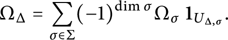 $$ \begin{align*} \Omega_\Delta = \sum_{\sigma \in \Sigma} (-1)^{\dim \sigma} \Omega_\sigma ~{\textbf 1}_{U_{\Delta, \sigma}}. \end{align*} $$
It is a $T_K$
-invariant complex measure on
$T_K$
-invariant complex measure on $X_{\Sigma }$
and corresponds to the function
$X_{\Sigma }$
and corresponds to the function $k_\Delta $
on
$k_\Delta $
on $N_{\mathbb R}$
. We think of it as a truncation of
$N_{\mathbb R}$
. We think of it as a truncation of $\omega _0$
with respect to the measures
$\omega _0$
with respect to the measures $\omega _\sigma $
at infinity. From Theorems 3.5 and 4.1, we have the following.
$\omega _\sigma $
at infinity. From Theorems 3.5 and 4.1, we have the following.
Proposition 6.1 Under the assumptions in Theorem 3.5 on the functions $K_\sigma $
, the total measure of
$K_\sigma $
, the total measure of $\Omega _\Delta $
is finite and is a polynomial in the support numbers of
$\Omega _\Delta $
is finite and is a polynomial in the support numbers of $\Delta $
.
$\Delta $
.
Remark 6.2 In fact, each tangent cone $T^-_{\Delta , \sigma }$
gives us an open neighborhood of the orbit closure
$T^-_{\Delta , \sigma }$
gives us an open neighborhood of the orbit closure $\overline {O}_\sigma $
in
$\overline {O}_\sigma $
in $X_{\Sigma }$
. To construct this open neighborhood, we complete
$X_{\Sigma }$
. To construct this open neighborhood, we complete $T^-_{\Delta , \sigma } \subset N_{\mathbb R}$
to an open subset
$T^-_{\Delta , \sigma } \subset N_{\mathbb R}$
to an open subset $\tilde {T}_{\Delta , \sigma } \subset X_{\Sigma }^+$
containing the closure
$\tilde {T}_{\Delta , \sigma } \subset X_{\Sigma }^+$
containing the closure $\overline {O^+_\sigma }$
by
$\overline {O^+_\sigma }$
by
 $$ \begin{align*}\tilde{T}_{\Delta, \sigma} = \bigcup_{\sigma': \sigma \preceq \sigma'} \bigcup_{\tau: \tau \preceq \sigma'} T^-_{Q_{\tau}, \sigma'} ~\subset X_{\Sigma}^+ := \bigsqcup_{\sigma \in \Sigma} N_{\mathbb R} / \operatorname{Span}(\sigma).\end{align*} $$
One verifies that $\tilde {T}_{\Delta , \sigma }$
is indeed an open subset of
$\tilde {T}_{\Delta , \sigma }$
is indeed an open subset of $X_{\Sigma }^+$
containing
$X_{\Sigma }^+$
containing $\overline {O^+_\sigma }$
. It follows that
$\overline {O^+_\sigma }$
. It follows that $\tilde {U}_{\Delta , \sigma } = \operatorname {Log}^{-1}(\tilde {T}_{\Delta , \sigma })$
is an open neighborhood of the orbit closure
$\tilde {U}_{\Delta , \sigma } = \operatorname {Log}^{-1}(\tilde {T}_{\Delta , \sigma })$
is an open neighborhood of the orbit closure $\overline {O}_\sigma $
in the toric variety
$\overline {O}_\sigma $
in the toric variety $X_{\Sigma }$
. We note that
$X_{\Sigma }$
. We note that $T^-_{\Delta , \sigma }$
is open dense in
$T^-_{\Delta , \sigma }$
is open dense in $\tilde {T}_{\Delta , \sigma }$
, and hence, for the purposes of truncation, it does not matter whether we work with
$\tilde {T}_{\Delta , \sigma }$
, and hence, for the purposes of truncation, it does not matter whether we work with $T^-_{\Delta , \sigma }$
or
$T^-_{\Delta , \sigma }$
or $\tilde {T}_{\Delta , \sigma }$
.
$\tilde {T}_{\Delta , \sigma }$
.
6.2 Combinatorial truncation as a Lefschetz number
In this section, we give an interpretation of the combinatorial truncation as a Lefschetz number.
6.2.1 Lefschetz number
Let X be a topological space such that all its cohomology groups $H^i(X, {\mathbb R})$
are finite dimensional and for some
$H^i(X, {\mathbb R})$
are finite dimensional and for some $n \geqslant 0$
,
$n \geqslant 0$
, $H^i(X, {\mathbb R}) = 0$
,
$H^i(X, {\mathbb R}) = 0$
, $\forall i> n$
. Let
$\forall i> n$
. Let $\Phi : X \to X$
be a continuous map. Recall that the Lefschetz number of
$\Phi : X \to X$
be a continuous map. Recall that the Lefschetz number of $\Phi $
is defined to be
$\Phi $
is defined to be
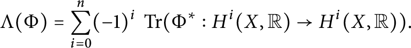 $$ \begin{align*} \Lambda(\Phi) = \sum_{i=0}^n (-1)^i ~\operatorname{Tr}(\Phi^*: H^i(X, {\mathbb R}) \to H^i(X, {\mathbb R})). \end{align*} $$
The Lefschetz number of the identity map is, by definition, equal to the Euler characteristic of X. The Lefschetz number appears in the Lefschetz fixed point theorem which states that if X is a compact triangulable space and $\Lambda (\Phi ) \neq 0$
, then
$\Lambda (\Phi ) \neq 0$
, then $\Phi $
has at least one fixed point.
$\Phi $
has at least one fixed point.
Let us define an analogue of the notion of Lefschetz number for morphisms of sheaves. Let ${\mathcal F}$
be a sheaf of vector spaces on X such that all the cohomology groups of
${\mathcal F}$
be a sheaf of vector spaces on X such that all the cohomology groups of $(X, {\mathcal F})$
are finite dimensional and for some n,
$(X, {\mathcal F})$
are finite dimensional and for some n, $H^i(X, {\mathcal F}) = 0$
,
$H^i(X, {\mathcal F}) = 0$
, $\forall i> n$
. By a morphism of sheaves
$\forall i> n$
. By a morphism of sheaves $\Psi : {\mathcal F} \to {\mathcal F}$
, we mean a collection of linear maps
$\Psi : {\mathcal F} \to {\mathcal F}$
, we mean a collection of linear maps $\{\Psi _U: {\mathcal F}(U) \to {\mathcal F}(U) : U \subset X \text { open }\}$
which are compatible with the restriction maps. That is, for
$\{\Psi _U: {\mathcal F}(U) \to {\mathcal F}(U) : U \subset X \text { open }\}$
which are compatible with the restriction maps. That is, for $U \subset V$
, we have
$U \subset V$
, we have
 $$ \begin{align*} \Psi_U \circ \operatorname{rest}_{V, U} = \operatorname{rest}_{V, U} \circ \Psi_V. \end{align*} $$
Clearly, $\Psi $
induces linear maps
$\Psi $
induces linear maps $\Psi ^*: H^i(X, {\mathcal F}) \to H^i(X, {\mathcal F})$
between the cohomology groups of
$\Psi ^*: H^i(X, {\mathcal F}) \to H^i(X, {\mathcal F})$
between the cohomology groups of $(X, {\mathcal F})$
. Extending the above notion of Lefschetz number, we make the following definition.
$(X, {\mathcal F})$
. Extending the above notion of Lefschetz number, we make the following definition.
Definition 6.1 (Lefschetz number for morphisms of sheaves)
The Lefschetz number $\Lambda (\Psi , {\mathcal F})$
is defined to be
$\Lambda (\Psi , {\mathcal F})$
is defined to be
 $$ \begin{align*} \Lambda(\Psi, {\mathcal F}) = \sum_{i=0}^n (-1)^i ~\operatorname{Tr}(\Psi^*: H^i(X, {\mathcal F}) \to H^i(X, {\mathcal F})). \end{align*} $$
Remark 6.3 When $\Psi $
is the identity morphism, i.e., all the maps
$\Psi $
is the identity morphism, i.e., all the maps $\Psi _U$
are identities, then
$\Psi _U$
are identities, then $\Lambda (\Psi , {\mathcal F})$
is just the Euler characteristic of the sheaf
$\Lambda (\Psi , {\mathcal F})$
is just the Euler characteristic of the sheaf ${\mathcal F}$
.
${\mathcal F}$
.
Let $\mathcal {U}$
be a finite open cover of X. Suppose
$\mathcal {U}$
be a finite open cover of X. Suppose $\mathcal {U}$
is a good open cover with respect to
$\mathcal {U}$
is a good open cover with respect to ${\mathcal F}$
, that is,
${\mathcal F}$
, that is, ${\mathcal F}$
is acyclic on any intersection of the open sets in
${\mathcal F}$
is acyclic on any intersection of the open sets in $\mathcal {U}$
. It is a standard result in topology that the Čech cohomology groups of
$\mathcal {U}$
. It is a standard result in topology that the Čech cohomology groups of $(\mathcal {U}, {\mathcal F})$
are independent of the choice of the good open cover and coincide with the sheaf cohomology groups of
$(\mathcal {U}, {\mathcal F})$
are independent of the choice of the good open cover and coincide with the sheaf cohomology groups of $(X, {\mathcal F})$
.
$(X, {\mathcal F})$
.
Suppose the vector spaces in the Čech cochain complex $C^\bullet (\mathcal {U}, {\mathcal F})$
are finite dimensional. In other words, for any collection of open sets
$C^\bullet (\mathcal {U}, {\mathcal F})$
are finite dimensional. In other words, for any collection of open sets $U_1, \ldots , U_k \in \mathcal {U}$
, we have
$U_1, \ldots , U_k \in \mathcal {U}$
, we have $\dim H^0(U_1 \cap \cdots \cap U_k, {\mathcal F}) < \infty $
. In this case, the Lefschetz number can be computed in terms of the traces of the vector spaces in the cochain complex
$\dim H^0(U_1 \cap \cdots \cap U_k, {\mathcal F}) < \infty $
. In this case, the Lefschetz number can be computed in terms of the traces of the vector spaces in the cochain complex $C^\bullet (\textrm {U}, {\mathcal F})$
as well. This straightforward result is sometimes referred to as the Hopf trace formula.
$C^\bullet (\textrm {U}, {\mathcal F})$
as well. This straightforward result is sometimes referred to as the Hopf trace formula.
Proposition 6.4 With assumptions as above, the Lefschetz number can be computed as
 $$ \begin{align*}\Lambda(\Psi) = \sum_{i=0}^n (-1)^i ~\operatorname{Tr}(\Psi^*: C^i(\mathcal{U}, {\mathcal F}) \to C^i(\mathcal{U}, {\mathcal F})),\end{align*} $$
where $C^i(\mathcal {U}, {\mathcal F})$
denotes the vector space of ith Čech cochains of
$C^i(\mathcal {U}, {\mathcal F})$
denotes the vector space of ith Čech cochains of $\mathcal {U}$
with coefficients in
$\mathcal {U}$
with coefficients in ${\mathcal F}$
.
${\mathcal F}$
.
Similarly, suppose X is equipped with a measure and ${\mathcal F}$
a sheaf of
${\mathcal F}$
a sheaf of $L^2$
-functions on X, and let
$L^2$
-functions on X, and let $\Psi : {\mathcal F} \to {\mathcal F}$
be a morphism of sheaves. Moreover, suppose for every open set U, the linear operator
$\Psi : {\mathcal F} \to {\mathcal F}$
be a morphism of sheaves. Moreover, suppose for every open set U, the linear operator $\Psi : {\mathcal F}(U) \to {\mathcal F}(U)$
is a trace class operator with kernel function
$\Psi : {\mathcal F}(U) \to {\mathcal F}(U)$
is a trace class operator with kernel function $K_U$
. Then, for each i, the induced map
$K_U$
. Then, for each i, the induced map $\Psi ^*: H^i(X, {\mathcal F}) \to H^i(X, {\mathcal F})$
is also a trace class operator. We denote its kernel by
$\Psi ^*: H^i(X, {\mathcal F}) \to H^i(X, {\mathcal F})$
is also a trace class operator. We denote its kernel by $T_i$
.
$T_i$
.
Definition 6.2 (Lefschetz number for morphisms of sheaves of
$L^2$
-functions)

We define the Lefschetz number $\Lambda (\Psi , {\mathcal F})$
by
$\Lambda (\Psi , {\mathcal F})$
by
 $$ \begin{align} \Lambda(\Psi, {\mathcal F}) = \int\limits_X \sum_{i=0}^n (-1)^i T_i(x) \, dx. \end{align} $$
As above, let $\mathcal {U}$
be a finite open cover of X which is a good cover with respect to
$\mathcal {U}$
be a finite open cover of X which is a good cover with respect to ${\mathcal F}$
. Suppose, for each i, the operator
${\mathcal F}$
. Suppose, for each i, the operator $\Psi ^*: C^i(\mathcal {U}, {\mathcal F}) \to C^i(\mathcal {U}, {\mathcal F})$
is trace class with kernel
$\Psi ^*: C^i(\mathcal {U}, {\mathcal F}) \to C^i(\mathcal {U}, {\mathcal F})$
is trace class with kernel $K_i$
. Similarly to Proposition 6.4, the Lefschetz number
$K_i$
. Similarly to Proposition 6.4, the Lefschetz number $\Lambda (\Psi , {\mathcal F})$
can be computed as
$\Lambda (\Psi , {\mathcal F})$
can be computed as
 $$ \begin{align*}\Lambda(\Psi, {\mathcal F}) = \int\limits_X \sum_{i=0}^n (-1)^i K_i(x) \, dx.\end{align*} $$
The observation in this section is that when $X=X_{\Sigma }$
is a toric variety, the Lefschetz number is given by a combinatorial truncation
$X=X_{\Sigma }$
is a toric variety, the Lefschetz number is given by a combinatorial truncation $J_{\Sigma }(\Delta )$
. As usual, let
$J_{\Sigma }(\Delta )$
. As usual, let $\Sigma $
be a (rational) fan in
$\Sigma $
be a (rational) fan in $N_{\mathbb R}$
, and let
$N_{\mathbb R}$
, and let $\Delta \in \mathcal {P}(\Sigma )$
be a polytope with normal fan
$\Delta \in \mathcal {P}(\Sigma )$
be a polytope with normal fan $\Sigma $
. As in Section 5.1, let
$\Sigma $
. As in Section 5.1, let $X_{\Sigma }$
be the toric variety of the fan
$X_{\Sigma }$
be the toric variety of the fan $\Sigma $
and
$\Sigma $
and $\mathcal {O}(D_\Delta )$
be the sheaf of sections of the (Cartier) divisor
$\mathcal {O}(D_\Delta )$
be the sheaf of sections of the (Cartier) divisor $D_\Delta $
associated with
$D_\Delta $
associated with $\Delta $
. Let the
$\Delta $
. Let the $a_\rho $
,
$a_\rho $
, $\rho \in \Sigma (1)$
, be the support numbers of
$\rho \in \Sigma (1)$
, be the support numbers of $\Delta $
. Let
$\Delta $
. Let $\Delta '$
be the polytope whose support numbers are the
$\Delta '$
be the polytope whose support numbers are the $a_\rho -1$
. Let
$a_\rho -1$
. Let $\Psi : \mathcal {O}(-D_{\Delta '}) \to \mathcal {O}(-D_{\Delta '})$
be a morphism of sheaves.
$\Psi : \mathcal {O}(-D_{\Delta '}) \to \mathcal {O}(-D_{\Delta '})$
be a morphism of sheaves.
Recall that the characters $\chi _m$
,
$\chi _m$
, $m \in M$
, form a vector space basis for
$m \in M$
, form a vector space basis for ${\mathbb C}[U_0]$
. Moreover, a subset of this basis is a basis for
${\mathbb C}[U_0]$
. Moreover, a subset of this basis is a basis for $\mathcal {O}(-D_{\Delta '})$
. For
$\mathcal {O}(-D_{\Delta '})$
. For $m \in M$
, let
$m \in M$
, let $K_\sigma (m)$
be the
$K_\sigma (m)$
be the $(m, m)$
-entry of the matrix of the linear operator
$(m, m)$
-entry of the matrix of the linear operator $\Psi _\sigma : \mathcal {O}(-D_{\Delta '})(U_\sigma ) \to \mathcal {O}(-D_{\Delta '})(U_\sigma )$
. The following follows from Section 5.2 and in particular (5.9).
$\Psi _\sigma : \mathcal {O}(-D_{\Delta '})(U_\sigma ) \to \mathcal {O}(-D_{\Delta '})(U_\sigma )$
. The following follows from Section 5.2 and in particular (5.9).
Proposition 6.5 (Combinatorial truncation as a Lefschetz number on a toric variety)
With notation as above, the Lefschetz number $\Lambda (\Psi , \mathcal {O}(-D_{\Delta '}))$
is equal to the truncated sum
$\Lambda (\Psi , \mathcal {O}(-D_{\Delta '}))$
is equal to the truncated sum $S_{\Sigma }(\Delta , M)$
:
$S_{\Sigma }(\Delta , M)$
:
 $$ \begin{align*}\Lambda(\Psi, \mathcal{O}(-D_{\Delta'})) = S_{\Sigma}(\Delta, M) := \sum_{m \in M} \sum_{\sigma \in \Sigma} (-1)^{\dim \sigma} K_\sigma(m)~ {\textbf 1}_{T^-_{\Delta, \sigma} \cap M}(m).\end{align*} $$
Remark 6.6 The reason for the appearance of the polytope $\Delta '$
instead of
$\Delta '$
instead of $\Delta $
is that we defined the outward tangent cones
$\Delta $
is that we defined the outward tangent cones $T^-_{\Delta , \sigma }$
using strict inequalities. If we change the convention and use nonstrict inequalities in the definition of
$T^-_{\Delta , \sigma }$
using strict inequalities. If we change the convention and use nonstrict inequalities in the definition of $T^-_{\Delta , \sigma }$
, then Proposition 5.9 holds with D in place of
$T^-_{\Delta , \sigma }$
, then Proposition 5.9 holds with D in place of $D'$
.
$D'$
.
Finally, as a side remark, we also mention an example of a presheaf that is reminiscent of Arthur’s construction of the kernels $K_P$
(see [Reference ArthurAr05, Section 4]).
$K_P$
(see [Reference ArthurAr05, Section 4]).
Example 6.7 (A sheaf of W-invariant sections on the toric variety of Weyl fan)
Suppose $\Sigma $
is the Weyl fan and hence the Weyl group acts on
$\Sigma $
is the Weyl fan and hence the Weyl group acts on $\Sigma $
. Note that by definition W acts on the character lattice M. For
$\Sigma $
. Note that by definition W acts on the character lattice M. For $\sigma \in \Sigma $
, let
$\sigma \in \Sigma $
, let $W_\sigma $
be the W-stabilizer of
$W_\sigma $
be the W-stabilizer of $\sigma $
. Let
$\sigma $
. Let $\mathcal {O}(\Delta )$
be the invertible sheaf associated with a W-invariant polytope
$\mathcal {O}(\Delta )$
be the invertible sheaf associated with a W-invariant polytope $\Delta $
. We define the sheaf
$\Delta $
. We define the sheaf $\mathcal {O}(\Delta )^W$
by
$\mathcal {O}(\Delta )^W$
by
 $$ \begin{align*}H^0(U_\sigma, \mathcal{O}(\Delta)^W) := H^0(U_\sigma, \mathcal{O}(\Delta))^{W_\sigma}, \quad \forall \sigma \in \Sigma.\end{align*} $$
Let $\tau \subset \sigma $
be cones in
$\tau \subset \sigma $
be cones in $\Sigma $
. Note that
$\Sigma $
. Note that $W_\sigma \subset W_\tau $
and hence if
$W_\sigma \subset W_\tau $
and hence if $f \in H^0(U_\sigma , \mathcal {O}(\Delta ))^{W_\sigma }$
, then, in general,
$f \in H^0(U_\sigma , \mathcal {O}(\Delta ))^{W_\sigma }$
, then, in general, $f_{|U_\tau }$
may not be
$f_{|U_\tau }$
may not be $W_\tau $
-invariant and hence may not lie in
$W_\tau $
-invariant and hence may not lie in $H^0(U_\tau , \mathcal {O}(\Delta ))^{W_\tau }$
. We remedy this by defining the restriction map
$H^0(U_\tau , \mathcal {O}(\Delta ))^{W_\tau }$
. We remedy this by defining the restriction map $i_{\sigma \tau }: H^0(U_\sigma , \mathcal {O}(\Delta )^W) \to H^0(U_\tau , \mathcal {O}(\Delta )^W)$
by:
$i_{\sigma \tau }: H^0(U_\sigma , \mathcal {O}(\Delta )^W) \to H^0(U_\tau , \mathcal {O}(\Delta )^W)$
by:
 $$ \begin{align*}i_{\sigma\tau}(f) = \sum_{w \in W_\tau/W_\sigma} (w \cdot f)_{|U_\tau}.\end{align*} $$
Let us verify that the above restriction maps $i_{\sigma \tau }$
give a well-defined presheaf on
$i_{\sigma \tau }$
give a well-defined presheaf on $X_{\Sigma }$
. Suppose we have cones
$X_{\Sigma }$
. Suppose we have cones $\gamma \subset \tau \subset \sigma $
in
$\gamma \subset \tau \subset \sigma $
in $\Sigma $
with corresponding affine charts
$\Sigma $
with corresponding affine charts $U_\gamma \subset U_\tau \subset U_\sigma $
. We need to show
$U_\gamma \subset U_\tau \subset U_\sigma $
. We need to show $i_{\tau \gamma } \circ i_{\sigma \tau } = i_{\sigma \gamma }$
. Let
$i_{\tau \gamma } \circ i_{\sigma \tau } = i_{\sigma \gamma }$
. Let $f \in H^0(U_\sigma , \mathcal {O}(\Delta )^W)$
. We have
$f \in H^0(U_\sigma , \mathcal {O}(\Delta )^W)$
. We have
 $$ \begin{align*}i_{\tau \gamma}(i_{\sigma \tau}(f)) = \sum_{w \in W_\gamma / W_\tau} \sum_{w' \in W_\tau / W_\sigma} (ww') \cdot f. \end{align*} $$
As w (resp. $w'$
) runs over a set of representatives for
$w'$
) runs over a set of representatives for $W_\gamma / W_\tau $
(resp.
$W_\gamma / W_\tau $
(resp. $W_\tau / W_\sigma $
), the product
$W_\tau / W_\sigma $
), the product $ww'$
runs over a set of representatives for
$ww'$
runs over a set of representatives for $W_\gamma / W_\sigma $
. This proves the claim.
$W_\gamma / W_\sigma $
. This proves the claim.
It is interesting to compute the Euler characteristic and Čech cohomologies of the above presheaf.
Acknowledgment
We would like to thank James Arthur, William Casselman, Mark Goresky, Thomas Hales, Erez Lapid, Werner Müller, and Tian An Wong for useful correspondences and conversations. We would also like to thank the referee for a careful reading of the manuscript.


 Open access