

1. Introduction
Discussions around the nature of phonological elements have recently centred around at least two issues, namely whether phonological features are substance-full or substance-free, and whether they are innate or emergent. These two debated dimensions render four logically possible combinations for the nature of phonological elements: innate substance-full (e.g., Optimality Theory: Prince and Smolensky Reference Prince and Smolensky1993 et seq.), innate substance-free (Chomsky and Halle Reference Chomsky and Halle1968, Hale and Reiss Reference Hale, Reiss, Burton-Roberts, Carr and Docherty2000 et seq.), emergent substance-full (perhaps Exemplar Theory: Pierrehumbert 2001 et seq.), and emergent substance-free (Boersma Reference Boersma1998 et seq., Blaho Reference Blaho2007, Iosad Reference Iosad2013). The first goal of the present article is to provide a learning algorithm for the “emergent substance-free view”. This would provide provisional support for that view, given that no learning algorithms have been proposed for the other three views, perhaps because such learning algorithms cannot exist. From the phonologist's standpoint, however, merely having a learning algorithm cannot suffice: language observation has established that humans exhibit featural behaviour. That is, human learners infer phonological features from experiencing phonetic input, or from experiencing morphological alternations, or from both (Hamann Reference Hamann2007). The second goal of the present article, therefore, is to investigate whether and how our substance-free learning algorithm leads to the emergence of phonological features (rather than, say, separate phonemes), and whether these features correspond to what phonologists tend to think they should.Footnote 1
If we assume that phonological features are innate – that is, that at the start of language acquisition every child is endowed with a universal set of phonological feature categories – the debate about whether these features intrinsically refer to phonetic substance or not is highly relevant. After all, if phonological features are innate, then there are only two logical possibilities: they either do or don't refer to phonetic substance, and this makes a large difference for phonological theory. If features are innate and do refer to phonetic substance, every human being's phonological module could contain a substance-specific innate constraint like *FrontRoundedVowel, allowing an innatist version of Optimality Theory (Prince and Smolensky Reference Prince and Smolensky1993) to provide a correct account of the phonological processing of things that correlate with what phoneticians would transcribe as [y] or [ø]. On the other hand, if features are innate and do not refer to phonetic substance, then phonological production will have to be a purely computational system that uses logical operations and/or set calculus to turn an incoming underlying form consisting of arbitrary units into a phonological surface form also consisting of arbitrary units (in the same or a different alphabet). Under that view, the innate phonological features could either be arbitrary labels (such as α or β) or they could still be the usual ones, with a “front rounded vowel” potentially correlating to something phoneticians would describe as [ɔ], [n] or [g], with the innate constraint *FrontRoundedVowel in effect militating against such sounds.
The innateness assumption is problematic when it comes to the learnability of the language-specific relations between phonological representations and their auditory or articulatory correlates: for example, a child has to learn how to relate a feature like /voice/ or /β/ to the myriad ways in which languages can implement what linguists like to call voicing (some of which have nothing to do with vocal fold vibration), but no proposals are known to us about how such links can be acquired (for an overview, see Boersma Reference Boersma, Cohn, Fougeron and Huffman2012). Hale and Reiss (Reference Hale, Reiss, Burton-Roberts, Carr and Docherty2000), for instance, propose the existence of an innate “transducer” that handles the linking, but Reiss (Reference Reiss, Hannahs and Bosch2017: section 15.7.4) acknowledges that it is not easy to implement such an instrument in the context of language-specific phonetic variability.
The linking problem is solved if we instead assume that phonological elements are emergent, that is, that they emerge from the language learner's interaction with the world. At the start of acquisition, then, the child's phonology has no knowledge of the outside world: the child's phonological behaviour shows no evidence yet of the existence of any features, any hierarchies, and any sets; this situation is substance-free almost by definition. During acquisition, the child's phonological module will come to interact with the phonetics and the morphology through the phonology–phonetics interface (which must exist, because humans comprehend and produce speech) and the phonology–morphology interface (which must exist in all languages that have morphology). A neural-network model that could implement these interactions is shown in Figure 1.
A schematic representation of the three modules and their two interfaces. Information can flow from meaning to sound (production), from sound to meaning (comprehension), or from sound–meaning pairs inwards (acquisition). The number of nodes and levels within each module is chosen arbitrarily for the purpose of this illustration.

During acquisition, while the phonology continues to contain no phonetic (or morphological) substance, it becomes strongly connected to both phonetic substance and morphological substance. So, the phonological module does not intrinsically refer to substance, but it becomes externally linked to substance during acquisition (this is consistent with Reiss’ definition of substance-freedom, which allows linking).Footnote 2 The first goal of this article, then, is to devise an artificial neural network that can simulate the acquisition of a toy language, that is, that learns, from experienced phonetic and/or morphological input, to produce and comprehend speech in a way that is appropriate for this language. Our subsequent research question (our second goal) is to investigate what kinds of featural behaviour the resulting network exhibits, and whether and how this emerged behaviour resounds with the way phonologists have been describing language behaviour in terms of phonological features. The article is organized as follows.
Section 2 introduces the toy language used in our simulations. The language has five possible utterances. Each of these utterances has a different composite meaning, which is a combination of a lexical and a numeric meaning. Each utterance is also systematically associated with a vowel sound, which is a combination of a first and second formant value.
Section 3 introduces the artificial neural networks. The nodes in the networks represent the sound level (basilar membrane frequencies), the meaning level (lexical and numeric morphemes), and an intermediate level that can be interpreted as a phonological surface structure. The information flow in the networks follows the tenets of the neural-network edition of the framework of Bidirectional Phonology & Phonetics (BiPhon-NN; see Boersma Reference Boersma2019, Boersma et al. Reference Boersma, Benders and Seinhorst2020), namely bidirectionality and parallelism.
Section 4 introduces the learning algorithm. The task of our virtual learners is to ultimately learn, from a large number of sound–meaning pairs, their language's mapping from sound to meaning (comprehension), as well as the mapping from meaning to sound (production). They do so by adapting the strengths of the connections between levels in response to incoming data, using a learning algorithm adopted from the field of machine learning (because it happens to be robust enough for our purposes), namely one of the Deep Boltzmann Machine learning algorithms (Salakhutdinov and Hinton Reference Salakhutdinov and Hinton2009).
Sections 5 through 7 present the simulations and their results. In each section we assess the results by first establishing that the network becomes a proficient speaker and/or listener of the target language, and by subsequently measuring the degree to which featural representations happen to emerge at levels away from the sound level and the meaning level, that is, at levels that we loosely identify as the phonological surface form (SF). In order to be able to establish which features come from the phonetics and which from the semantics, we first investigate what features emerge if a learner has access to sound alone (section 5) or to meaning alone (section 6), before proceeding to learners that have access to both (section 7).
In section 5, the virtual learners learn from sound alone. An essential requirement for meaningful later measurements at SF is that discrete categorical behaviour emerges in a humanlike way at SF, that is, the network should at some developmental stage exhibit “perceptual magnetism” (Kuhl Reference Kuhl1991) and the network should end up in a stage where incoming sounds lead to only five possible different activity patterns in the nodes of SF. These conditions are met, and we witness the emergence of three “shared” phonological features (i.e., shared between at least two different utterances), all of which can be traced back to shared auditory cues in the sounds.
In section 6, the virtual learners learn from meaning alone. Again, categorical behaviour happens to emerge at SF; that is, the five different possible meanings lead to five different activity patterns in the nodes of SF. Here we witness the emergence of four shared phonological features, all of which can be traced back to shared morphemes.
In section 7, the virtual learners finally learn from pairs of sound and meaning. An essential requirement for deciding that the phonological system has matured is that the resulting network can produce an intended meaning as the appropriate sound, and that it can comprehend an incoming sound as the appropriate meaning. These conditions are met: the network indeed becomes a good speaker as well as a good listener. The number of shared phonological features that emerges here is five: it is the union of the three phonetically based features of section 5 and the four semantically based features of section 6, with the two features that have both phonetic and semantic correlates ending up as stronger than the one feature that is based only on sound and the two features that are based only on meaning.
When comparing (in section 8) the results of sections 5 through 7, we conclude that features tend to emerge both from regularities in the sound (e.g., in cases in which some utterances have an identical formant value) and from regularities in the meaning (e.g., in cases in which some utterances have an identical lexical meaning or an identical numeric meaning), and that features emerge most strongly if they correspond to correlated regularities in sound and meaning, that is, if morphological alternations correspond to phonetic contrasts. For the substance-freedom debate this means that phonological features tend to come to be linked to auditory and semantic substance, even though such links are not built into the brain from the start but instead emerge from incoming data. Phonological representations, therefore, are devoid of phonetic substance, in exactly the same way as they are (uncontroversially, perhaps) devoid of semantic substance, although they are externally linked to phonetic representations in exactly the same way as they are (again uncontroversially, perhaps) externally linked to semantic representations. These linkages ensure that phonetic and semantic considerations can exert their pull on the phonology, although the phonological representations themselves are substance-free.
2. Toy language: An ideally distributed five-vowel inventory with alternations
This section presents the toy language that forms the basis of our simulations. The goal of a learner of this language is to acquire both production and comprehension, namely to map an intended meaning onto a sound that is appropriate for the language, as well as to map an incoming sound onto a meaning that is appropriate for the language.
Our toy language is a language that a linguist would describe as having five morphemes (or atomic meanings, from the phonologist's standpoint),Footnote 3 five words, and five vowels, in which morphological alternations correspond to vowel height variations. The learner of this language has access to less than that: the only input she receives consists of the atomic meanings and the formant values, and she will create a phonological interpretation on the basis of this morphemic (i.e., semantic) and phonetic input. We discuss, therefore, how the morphological and phonetic properties of this language might promote the emergence of featural representations in the learner. The simulations of later sections test how these predictions are borne out.
2.1 Utterances and words of the ambient language
Our toy language is a language with only five possible utterances. Each of these utterances consists of a single word. The possible words (and therefore the possible utterances) are written as the arbitrary (but mnemonic) notations a, e, i, o and u. These five possible words have different meanings, namely roughly ‘grain’, ‘egg’, ‘eggs’, ‘goat’ and ‘goats’, respectively. The words are also pronounced differently, namely roughly as [a], [e], [i], [o] and [u], respectively (hence their mnemonic notations).
2.2 Semantic representations in the ambient language
We assume that the semantics of the ambient language encodes grammatical number, that is, the singular–plural distinction. Four of the five words, namely the count nouns, therefore have a composite meaning, divided into a lexical meaning and a numeric meaning, as summarized in Table 1.
The meanings (morphemes) of the five possible words

Access by the child. The present article, which focuses on phonological rather than semantic learning, holds the strongly simplifying assumption that the child has access to the five meanings throughout her acquisition period, that is, that the child, given an utterance (though not the label of that utterance, as given in the first column of Table 1), can perform a correct semantic (or morphological) analysis of what is being said, even before her learning starts. See section 7.4 for discussion.
2.3 Phonological representations in the ambient language
When looking at these data from a morphophonological perspective, one would probably say that this language encodes grammatical number as a phonological height alternation (i.e., singulars with mid vowels have plurals with high vowels). Adult speaker–listeners of this toy language could represent the five words either in terms of phonemes or in terms of phonological features. Table 2 lists an example of each of the two types of phonological representation, for each word.
Potential adult phonological representations of the five possible words (inaccessible to the child)

As one potential example of phonemic representation, the second column of Table 2 shows five arbitrary labels (“arbitrary” in the sense that we mean the five letters to be mnemonic devices for linguists like ourselves only; they are not meant to have an essentialist status across speakers). The third column shows (equally arbitrary and mnemonic) potential featural representations. Here we choose to use the traditional binary phonological features /high/, /low/ and /back/, with a modest amount of underspecification: the high vowels are not specified in the table for /low/, because /+high/ can be understood to entail /–low/; the low vowel is similarly not specified in the table for /high/, because we assume that /+low/ entails /–high/; the low vowel is underspecified for /back/, because it actually is neither /+back/ nor /–back/. Other featural specifications are possible (the phonological literature is full of proposals), and it is not our intention to commit to any of these; in fact, the featural specifications in ambient adult speakers are irrelevant to our simulations, because our virtual infants will not have direct access to these specifications; instead, they will figure out their own specifications while they are acquiring the language.
Relating the semantic information in Table 1 to the phonological representations in Table 2 already reveals an advantage of the featural representations over the phonemic representations: only the featural specifications make it possible to encode (presumably in the lexicon) the two numeric meanings of Table 1 phonologically, for instance as /+high/ ‘pl’ and /–high/ ‘sg’. The featural specification thus expresses a generalization that is missed by the phonemic representation, which renders the number alternation suppletive and phonologically arbitrary (with number represented in terms of /high/, the three lexical meanings become /–low, –back/ ‘egg’, /–low, +back/ ‘goat’, and /+low/ ‘grain’). Our simulations in section 7.4 will test the prediction that the nature of systematic morphological alternation in the input data influences what featural representations virtual learners will arrive at. In terms of the toy language presented here, the specific prediction is that learners of our toy language, in which the numeric alternation correlates with an F1 difference, will create different phonological features than learners of a toy language in which the numeric alternation anticorrelates with an F1 difference (e.g., when ‘egg’ is /e/ and ‘eggs’ is /i/, as in our toy language, but ‘goat’ is /u/ and ‘goats’ is /o/, which is opposite to what our toy language does).
Access by the child. The present article assumes that the child has no access at all to any of the ambient phonological elements proposed in Table 2.
2.4 Phonetic implementations in the ambient language
As the learners need to learn sound–meaning mappings and have no direct access to the vowels’ phonological representations, the phonetic realizations of these vowels form an essential component of the acquisition of the language. Table 3 lists the ambient sounds of the five words. For simplicity reasons, we consider only the first formant (F1) and the second formant (F2) of each of the five vowels. The formant frequencies are in “auditory” values along the ERB (Equivalent Rectangular Bandwidth) scale (rather than in “acoustic” values in Hz), in order to correlate linearly with locations along the basilar membrane in the human inner ear.
The sounds of the five possible words

In order that our simulations will not be distracted by irrelevant properties of our toy language, we included quite some idealized symmetry in the inventory of Table 3. Thus, while in real languages the [a]–[e] distance is sometimes smaller or greater than the [e]–[i] distance, the three vowel heights of our toy language are equidistant with respect to F1, with adjacent heights spaced 3.0 ERB apart; in this way, no distance differences will influence our results. Something similar goes for F2: the F2 values of the five vowels [u]–[o]–[a]–[e]–[i] rise in equal steps of 3.0 ERB. A detail to note is that the F2 of [i] (3271 Hz) is higher than any acoustic F2 usually measured, but this value does correspond to the auditory second peak of [i], which is a combination of F3 and F4 (Flanagan Reference Flanagan1972). A deliberate detail of our toy language is that the F1 of [a] happens to be equal to the F2 of [u] (in real languages, the F1 of [a] is often higher or lower than the F2 of [u]); this detail will enable our simulations to tease apart the influence of phonetic similarities that are or are not supported by morphological alternations (see section 7.3).
A comparison between the phonemic and featural representations in Table 2 now reveals another advantage of the latter, when we relate them to the phonetic specifications in Table 3. An advantage of featural representations is that they could explain why the two high vowels have the same F1: with the feature /high/, a speaker would use a single strategy like “pronounce /+high/ with an F1 of 7.0 ERB”. With phonemic representations, a speaker would have to use “pronounce /i/ with an F1 of 7.0 ERB” as well as “pronounce /u/ with an F1 of 7.0 ERB”, but the equality of the two F1 values would be a coincidence: /i/ could just as well have an F1 of 6.5 ERB and /u/ an F1 of 7.5 ERB. Our simulations in sections 5 and 7 will test the prediction that a learner is more likely to create featural representations where vowels share an F1 (or F2) value than where they do not.
Access by the child. The present article assumes that the child has full access to the two formants of ambient utterances. As section 2.4 argues, these formants are not always the ones listed in Table 3.
2.5 Distribution of utterances in the ambient language
The task of our virtual learner is to learn the mapping from sound to meaning, as well as the mapping from meaning to sound, from a large number of given sound–meaning pairs spoken by adult speakers in her environment, where “sound” consists of a combination of an F1 value and an F2 value, and “meaning” consists of a combination of a lexical meaning and a numeric meaning. Both meaning and sound vary in the ambient language.
Each of the five composite meanings of Table 1 is equally common in language use, so that the adult speaker chooses each of the possible utterances a, e, i, o and u equally often, that is, in 20 percent of cases. The speaker realizes the intended utterance as an F1–F2 pair on the basis of Table 3.Footnote 4 However, the formant values in Table 3 are averages only: speakers draw each vowel token that they want to produce from a normal distribution in F1–F2 space, with the values in the table as its mean, and with a standard deviation of 1.0 ERB for both F1 and F2 independently (i.e., without covariation between F1 and F2). One hundred random realizations of utterances by a speaker could thus be distributed in an F1–F2 space as in Figure 2. Ten random realizations by ten speakers each could also be distributed as in Figure 2, as we simplifyingly ignore between-speaker variation (and therefore do not have to model speaker normalization by listeners).
One hundred randomly generated intended ambient utterances and their auditory realizations

Access by the child. The present article assumes that the child has full access to the two formants of ambient utterances, without being given the labels of the utterances. That is, we assume that the child, throughout the phonological acquisition period under consideration here, has a fully developed auditory system, including an appropriate low-level cortical representation of the frequency spectrum of the incoming sound.
3. Structure of the network
The most extensive neural networks used in the simulations of this article have to become listeners as well as speakers of our toy language. These networks contain the three levels illustrated in Figure 1: an auditory-phonetic level, a morphological (meaning) level, and something in between that we like to interpret as an emergent phonological level (in sections 5 and 6 we investigate even smaller architectures, namely sound and phonology alone, and meaning and phonology alone, respectively). This section discusses the types of representation that can be found on each of these levels and how they relate to the properties of the toy language and, thus, the input that our virtual learners will receive.
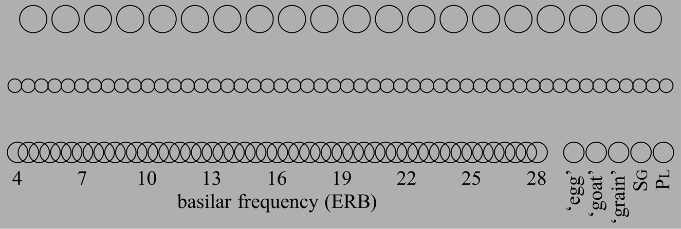
3.1 Auditory input level
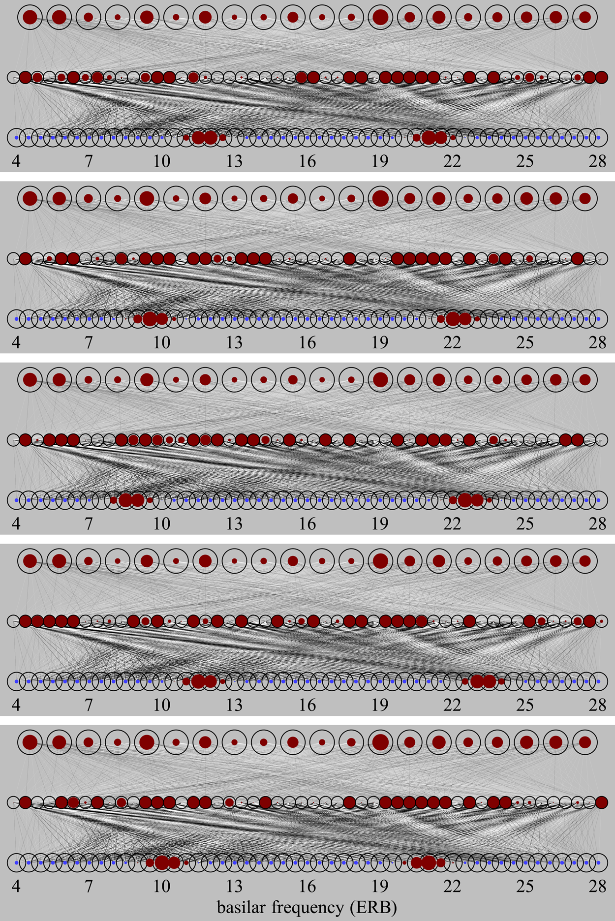
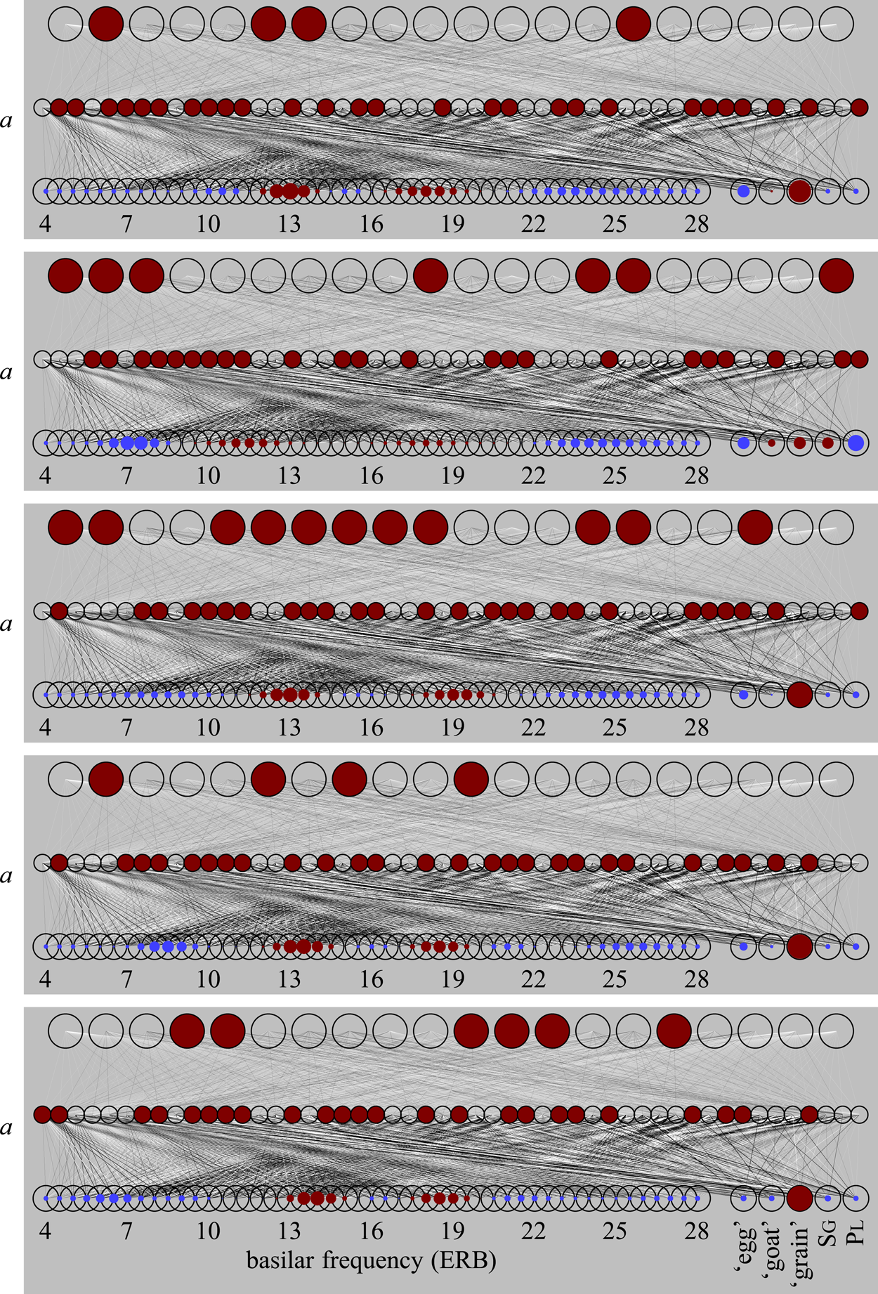
The Auditory Form is a representation of the part of the basilar membrane that is relevant for hearing F1 and F2: it is a spectral continuum running from 4.0 to 28.0 ERB. We discretize the continuum into 49 nodes, spaced 0.5 ERB apart,Footnote 5 so that node 1 is at 4.0 ERB and node 49 is at 28.0 ERB. Whenever an utterance comes in, it causes two Gaussian bumps on the basilar membrane with half-widths (standard deviations) of 0.68 ERB (as in Boersma et al. Reference Boersma, Benders and Seinhorst2020). Figure 3 shows the basilar activations of the five “standard utterances”, that is, the average utterance tokens whose F1 and F2 values are listed in Table 3. We can see that the standard tokens of the utterances i and u have an identical F1, as have the standard tokens of e and o. The constant auditory spreading on the basilar membrane (0.68 ERB) is reflected in the visual widths of the bumps, which are always the same.
Auditory input representations for a learner who listens to the five possible ambient utterances, produced with average F1 and F2 values. The (mostly big) dark red disks depict positive activity (the bigger the disk, the larger the activity, with a fully filled circle depicting an activity of +5), whereas the (usually smaller) light blue disks depict negative activity.

More realistically, the virtual learners will be confronted with phonetic variation. Figure 4 shows the auditory representations of three replications of each of the five utterances, which were randomly drawn from the auditory distribution described in section 2.4. We see the influence of the ambient standard deviation of 1.0 ERB, in that the three bumps for the same intended ambient utterance are at different locations.
Typical auditory input representations for a learner who listens to the five possible ambient utterances, each repeated three times with random variation in F1 and F2 (any visible correlations or anticorrelations between F1 and F2 values are purely coincidental).

3.2 Semantic input level
The input level for the five morphemes is simpler than the auditory level, because we implement no Gaussian bumps: each morpheme has its own node. Figure 5 shows the activities at this level for the five possible utterances a, e, i, o and u. The activity of a node that “belongs” to the meaning of the utterance is +4.5 (for the utterance with one node switched on, namely a) or +3.5 (for the utterances with two nodes switched on, namely the other four). There is a modest amount of normalization (or lateral inhibition): the nodes that are not switched on have a negative activity of −1, (if suppressed by one on node) or −2 (if suppressed by two on nodes).
Semantic input representations for a learner who listens to the five possible ambient utterances.

3.3 Deep levels
Figure 6 shows (against a background of grey matter) an example of the full network. The goal of this network is identical to the goal of the learner. That is, if the network is given a sound from the language while it is given no meaning, the network should construct the target-language-appropriate meaning (comprehension), and if the network is given a meaning from the language while it is given no sound, the network should construct the target-language-appropriate sound (production). Thus, the network should be able to construct the whole sound–meaning pair on the basis of sound or meaning alone.
Network structure. In this figure and many others, the numbers from 4 to 28 are basilar frequencies expressed in ERB; they apply only to the bottom left row of nodes.

In Figure 6, the input level at the bottom consists of the 49 auditory input nodes and the five semantic input nodes, drawn here in on separate “slabs” to illustrate their different roles in linguistics (the spreading and learning algorithms do not make this distinction; from their viewpoint there are simply 54 indiscriminate input nodes). The middle level consists of 50 nodes (this number is rather arbitrary, but should be high enough to allow for distributed representations); the input level is linked to it via a layer of connection weights that can be either positive (excitatory, here drawn in black) or negative (inhibitory, here drawn in white). These connection weights are determined slowly in the course of learning, and in this example are typical of a network that has been trained on 10,000 sound–meaning pairs (see section 7.1). The top level consists of (an again arbitrary number of) 20 nodes; it is connected to the middle level via a layer of connection weights that here are somewhat weaker (shown as thinner lines) than those of the lower layer (i.e., those between the input and middle levels). The weakness of the connections in the upper layer derives, in this example (but the effect is typical), from the fact that the learner has acquired suitable connection weights in the lower layer first, because that layer is closer to the input level.
The network in Figure 6 is called a deep artificial neural network (Hinton and Salakhutdinov Reference Hinton and Salakhutdinov2006) because it contains more than two levels of nodes (namely, three), or, equivalently, more than one layer of connections (namely, two).
The levels above the input level play a crucial rule in processing. The semantic input representations that can be seen to be activated in Figure 6 are ‘goat’ and pl, a combination that according to Table 1 can be expressed with the utterance u. This is confirmed by the two areas that are activated in the auditory input representation, which can be seen to lie around 7 and 13 ERB, which according to Table 3 is indeed typical of the utterance u. This is a typical situation for a fully trained network: the phonetic and semantic representations have come to reflect the statistics behind the sound–meaning pairings that the learner has received during training. The two directions of processing work with activity spreading, according to equations (1), (2), (3), usually (9), and sometimes (10) and (11) below, as explained in detail where it is relevant in sections 4, 5.3, 5.4, 6.3, 7.2 and 7.3. This basically works as follows. To produce the meaning ‘goats’, we activate the semantic nodes ‘goat’ and pl, spread this activity through the connections to the middle level, then from there to the top level, then from there back to the middle level, and from there to the auditory bottom level. After this up-and-down spreading is repeated several times (to allow for parallelism effects; see below), the activity at the auditory input level comes to settle around 7 and 13 ERB: the network has become a good speaker of the ambient language. Conversely, an incoming [u]-like sound will have bumps of activity for auditory nodes around 7 and 13 ERB, and to interpret this sound, the network spreads this activity to the middle level, then the top level, then the middle level again, and from there to the semantic bottom level. After this up-and-down spreading is repeated several times, the activity at the semantic bottom level comes to settle at ‘goat’ and pl: the network has become a good listener of the ambient language. In sum, the learner has become bidirectionally proficient: both production and comprehension have become successful.
Two properties of our network are crucial for establishing compatibility with earlier results in the Optimality-Theoretic (OT) modeling of parallel bidirectional phonology and phonetics (BiPhon; Boersma Reference Boersma2007, Reference Boersma, Boersma and Hamann2009): bidirectionality and parallelism. Bidirectionality means that production and comprehension employ the same grammatical elements, which in BiPhon-OT are globally ranked constraints and here in BiPhon-NN are the weighted connections that, as describe above, are used both for production and comprehension. Parallelism means that “later” considerations in processing can influence “earlier” considerations, for example that the “earlier” mapping from sound to phonological categories in comprehension can be influenced by the “later” access to the lexicon (Boersma Reference Boersma, Boersma and Hamann2009: section 7.1), and that the “earlier” mapping from morphemes to underlying forms in production can be influenced by “later” phonotactic biases (Boersma and Van Leussen Reference Boersma and Van Leussen2017); parallelism effects are expected to be enabled by our network through the process of “settling” described above: multiple up-and-down spreading until an equilibrium is reached can guarantee that in comprehension, for instance, the obtained phonological representation can potentially influence the incoming sound itself, as we will see happening in sections 5.4 and 7.3.
4. The learning procedure
In sections 5, 6, and 7, our network learns from sound, from meaning, or from both (respectively). In all three cases, learning consists of initializing the network to a random and weak initial (“infant”) state, and then executing a number of learning steps. This section describes all the equations that we used in our simulations of activity spreading and of learning, so that the reader will be able to replicate all our simulations, figures and tables, given also the means and standard deviations of the distributions (sections 2.3, 2.4, 3.1, 3.2). In other words, our simulations involve no “magic” outside of the formulas and numbers presented in this article.
In the initial state, then, the biases (resting excitations) of all nodes (i.e., a k, b l and c m,,,,,,,,, defined, below) are set to zero, and the weights (connection strengths) between all connected nodes (i.e., u kl and v lm defined below) are also set to zero. In other words, all parameters that constitute the long-term memory of the network are set to zero at the start of language acquisition.
A learning step starts by setting the activities of all nodes (i.e., the short-term memory of the network; x k, y l and z m, defined below) to zero. Next, we apply one piece of data to the network, by either:
• applying a sound input to the 49 auditory nodes on the bottom level (section 5), or
• applying a meaning input to the five semantic nodes on the bottom level (section 6), or
• applying a sound–meaning input pair to the 54 nodes on the bottom level (section 7).
Such an input directly determines the bottom-level activities x k, where k runs from 1 to K, where K is the number of input nodes (49, 5 or 54). Learning then takes place according to an algorithm that gradually changes the weights of the connections. We could have used any learning algorithm that can handle association, that is, any learning algorithm that is basically Hebbian in its strengthening of the connections between nodes that fire together (Hebb Reference Hebb1949, Kohonen Reference Kohonen1984). As the association has to be symmetric (we should be able to go from sound to meaning as easily as from meaning to sound), we prefer the learning algorithm to be symmetric as well: the influence of node A on node B has to equal the influence of node B on node A, both in activity spreading and in weight updating. The inoutstar algorithm used by Boersma et al. (Reference Boersma, Benders and Seinhorst2020) satisfies these requirements, but we found that it is not very robust for the present case. Following Boersma (Reference Boersma2019), the present article therefore applies a learning algorithm that has been proposed for Deep Boltzmann Machines (Salakhutdinov and Hinton Reference Salakhutdinov and Hinton2009, Goodfellow et al. Reference Goodfellow, Bengio and Courville2016: 661), which is a generalization from algorithms for Restricted Boltzmann Machines (Hinton and Sejnowski Reference Hinton and Sejnowski1983, Smolensky Reference Smolensky, Rumelhart and McClelland1986, Hinton Reference Hinton2002).Footnote 6 We go through the exact sequence of four phases employed by Boersma (Reference Boersma2019):
The initial settling phase. During this phase, the input nodes stay clamped at the activities that we just applied (as a sound, as a meaning, or as a sound and a meaning); that is, their activities stay constant throughout the learning step. We first spread activities from the bottom level x k to the middle-level activities y l, where l runs from 1 to L, which is the number of nodes on the middle level (i.e., L = 50):
 $$y_l\leftarrow \sigma \left({b_l + \mathop \sum \limits_{k = 1}^K x_ku_{kl} + \mathop \sum \limits_{m = 1}^M v_{lm}z_m} \right)$$
where σ( ) is the logistic function defined as
 $$\sigma ( x ) : = 1/( {1 + {\rm exp}( {-x} ) } ) $$
In (1), u kl is the weight of the connection from bottom node k to middle node l; z m are the activities of the top level (which are still zero in this first round), and v lm is the weight of the connection from middle node l to top node m, where m runs from 1 to M, which is the number of nodes on the top level (i.e., M = 20). Finally, b l is the bias of node l on the middle level. What (1) means is for each node on the middle level, its excitation (the expression between the parentheses) is computed by adding to the node's bias the sum of the contributions of all input nodes (and all top-level nodes), where input nodes (or top nodes) that are more strongly connected to this middle node have a larger influence. The action performed by the logistic function is that the activity of each node on the middle level is limited to assuming values between 0 (for large negative excitations) and 1 (for large positive excitations); if a node's excitation is 0, its activity becomes 0.5.
After (1), the next step is to spread activity from the middle level to the top-level nodes m:
 $$z_m\leftarrow \sigma \left({c_m + \mathop \sum \limits_{l = 1}^L y_lv_{lm}} \right)$$
where c m is the bias of node m on the top level.
The sequence of steps (1) and (3) is repeated 10 times, causing the network to end up in a near-equilibrium state. Note that the same connections v lm are used to spread activity from the middle to the top level, like in (3), as from the top to the middle level, like in (1) (except the first time, when z m is still zero). Thus, the connections are bidirectional.
The Hebbian learning phase. All connection weights and biases are changed according to a Hebbian learning rule, which implements the idea of fire together, wire together that the human brain and human neurons seem to follow (James Reference James1890, Hebb Reference Hebb1949):
 $$a_k\leftarrow a_k + \eta x_k$$
 $$b_l\leftarrow b_l + \eta y_l$$
 $$c_m\leftarrow c_m + \eta z_m$$
 $$u_{kl}\leftarrow u_{kl} + \eta x_ky_l$$
 $$v_{lm}\leftarrow v_{lm} + \eta y_lz_m$$
where η = 0.001 is the learning rate and a k is the bias of node k on the input level. What (4), (5) and (6) say is that the bias of a node is increased if the node is activated. For instance, if a node has a bias of 0.5430 and it receives an activity of +0.7, then the bias will rise to 0.5430 + 0.7 ⋅ 0.001 = 0.5437. What this entails for the future of this node is that the node will become a bit more active than it is now when, in the future, it again receives the same input, as per (1) and (3). Globally, the changes in the biases tend to enlarge the future differences between the nodes in the network. What (7) and (8) say is that the weight of a connection between two nodes is increased when both nodes are activated. For instance, if the connection weight between nodes A and B is 0.24600, and nodes A and B receive activities of 0.6 and 0.8, respectively, then the weight will rise to 0.24600 + 0.001⋅0.6⋅0.8 = 0.24648. This is the definition of Hebbian learning: it entails for the future of the two nodes that (for example) node A will become more active than it is now when node B is again activated in the future, as per (1) and (3). Globally, the connections between nodes that are active together now tend to become stronger, so that they are more likely to become active together in the future. Taking the biases and weights together, one can abbreviate the role of (4) to (8) as: “if two nodes fire together, they tend to wire together, which makes it more likely that in the future they will fire together even more.”
However, the desired stability of the learning algorithm requires that these two true learning phases are complemented by two unlearning phases.
The dreaming phase. We now unclamp the input level; that is, we allow it to go free. The bottom level of the network will receive a new state that is no longer directly based on what has just been heard. The first step, therefore, is to spread activities from the middle level to the bottom level:
 $$x_k\leftarrow a_k + \mathop \sum \limits_{l = 1}^L u_{kl}y_l$$
where a k is the bias of node k on the bottom level. Again, we see that the weights u kl of the bottom layer are used both bottom-up, as in (1), and top-down, as in (9). Next, we compute new activities on the middle and top levels:
 $$z_m\;\sim \;{\cal B}\left({\sigma \left({c_m + \mathop \sum \limits_{l = 1}^L y_lv_{lm}} \right)} \right)$$
 $$y_l\;\sim \;{\cal B}\left({\sigma \left({b_l + \mathop \sum \limits_{k = 1}^K x_ku_{kl} + \mathop \sum \limits_{m = 1}^M v_{lm}z_m} \right)} \right)$$
where  ${\cal B}( \;) $ is the Bernoulli distribution. For instance, the equation $z\;\sim \;{\cal B}( p ) $ will put into z the number 1 with probability p, and the number 0 with probability 1 − p. This is needed to bring some randomness, that is, free-roving associations, into this virtual brain.
The sequence from (9) through (11) is performed 10 times. to arrive at a near-equilibrium again.
The anti-Hebbian learning phase. In this final phase we unlearn from the dreamed-up network state:
 $$a_k\leftarrow a_k-\eta x_k$$
 $$b_l\leftarrow b_l-\eta y_l$$
 $$c_m\leftarrow c_m-\eta z_m$$
 $$u_{kl}\leftarrow u_{kl}-\eta x_ky_l$$
 $$v_{lm}\leftarrow v_{lm}-\eta y_lz_m$$
What (12) through (16) do in the long run is that the virtual brain unlearns a bit of the states that it already “knows”, namely the states that it can visit by roving randomly through the space of its possible states. Together with the Hebbian learning phases, the virtual brain slowly replaces a bit of its existing average knowledge with a bit of incoming knowledge. On average, the dwindling knowledge and the new knowledge are of comparable sizes. Once the virtual brain has fully learned from its environment, and the environment does not change, the Hebbian learning phase and the anti-Hebbian learning phase cancel each other out (on average), and learning stops.
The whole procedure of the four phases – 10 times (1) through (3), once (4) through (8), 10 times (9) through (11), and once (12) through (16) – is repeated up to 10,000 times, each time with a new sound (section 5), a new meaning (section 6), or a new sound–meaning pair (section 7). These 10,000 learning steps constitute the learning procedure of our virtual brain, from infancy to maturity; the brain starts in a randomly and weakly connected initial state and ends up in a moderately advanced state, though not in a final equilibrium state of learning, which might take a million steps. In our examples, the number of learning steps that the networks that we show have gone through is most often 3,000 (for a moderately trained network that shows some properties known from acquisition studies) or 10,000 (for a thoroughly trained network).
5. Creating categories from sound alone
In order to be able to identify which of the features that will emerge from sound–meaning learning in section 7 are phonetically based, we first establish what features emerge if a learner confronted with our toy language has access only to the sounds, and not to any meanings.
5.1 Language environment
For the learner with no knowledge of meaning, the utterances of Figure 2 come without any intended phonological or semantic representation. That is, this learner is confronted with only F1 and F2 values, as in Figure 7.
The utterances from Figure 2 as they come to a sound-only learner.
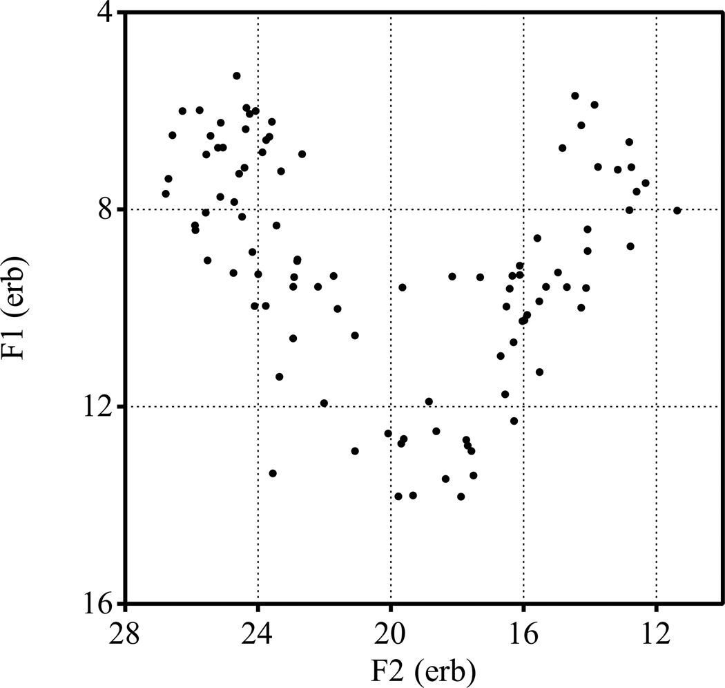
A learner faced with such a pooled auditory input distribution has to figure out that the sound tokens (the dots in Figure 7) were drawn from not more and not fewer than five categories. Superficial inspection of Figure 7, which shows little visual clustering, suggests that this may be difficult if the whole input set consists of only 100 tokens. With 1000 tokens, however, the pooled auditory representation may look like Figure 8, which exhibits clear visual clustering. A comparison of Figures 7 and 8 suggests that our simulations of auditory distributional learning may require thousands of tokens randomly drawn from the language environment.
The overt realizations of one thousand random utterances.

The sound-only virtual learner thus hears only the unlabeled sound data from the type shown in Figure 7 or Figure 8, never any labelled data as in Figure 2. It is the learner herself who may or may not figure out that the language has five phonemes (or three heights and two or three backness values).
5.2 The network before and after learning
For learning from sound alone, we use the network in Figure 9, where the input (bottom) level consists of 49 auditory nodes only, with basilar frequencies rising from 4 to 28 ERB, from left to right. The other two levels have no initial interpretation, and their visual ordering in the Figure represents no physical ordering.
The initial state of a network that can learn from a distribution of sounds.

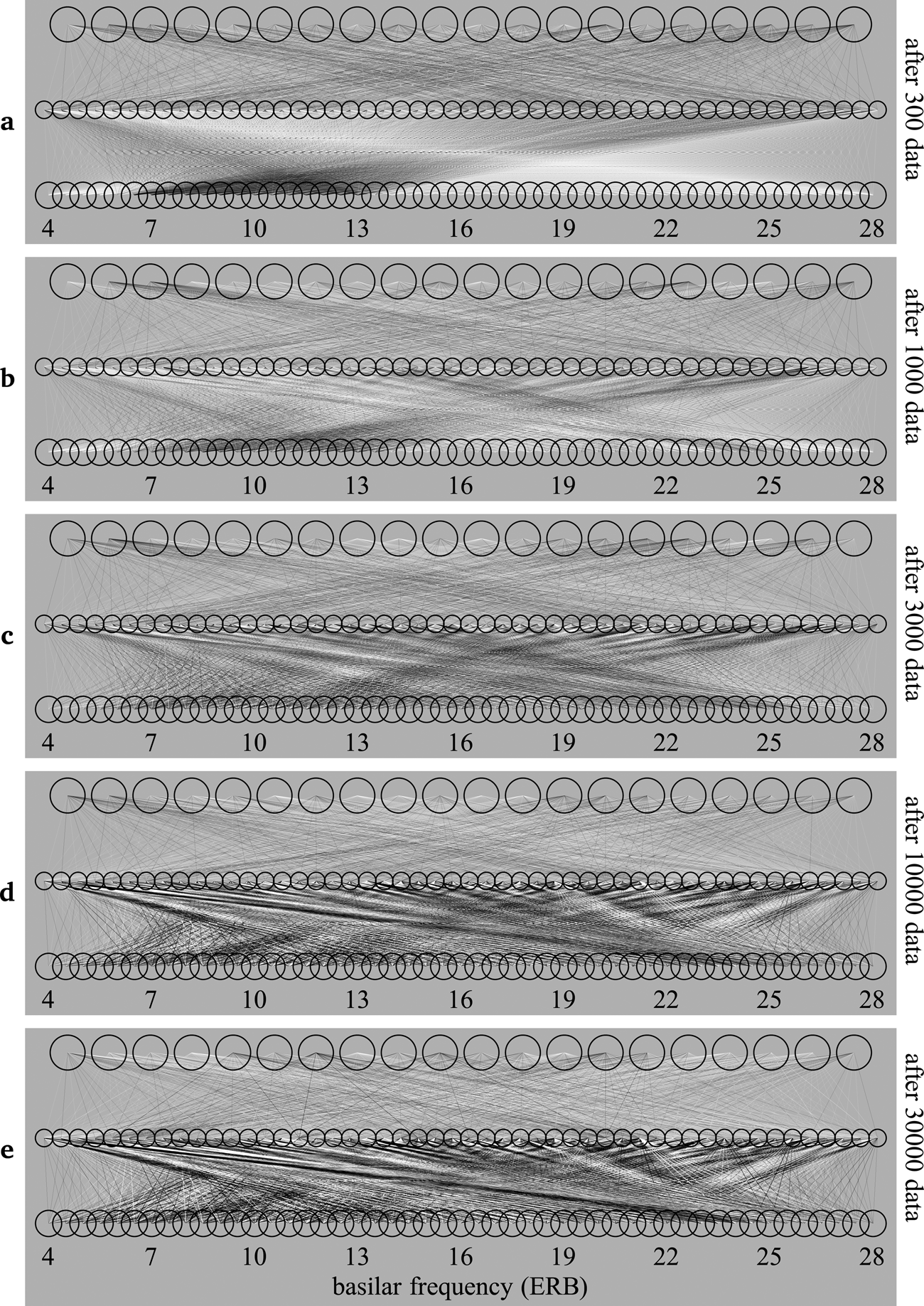
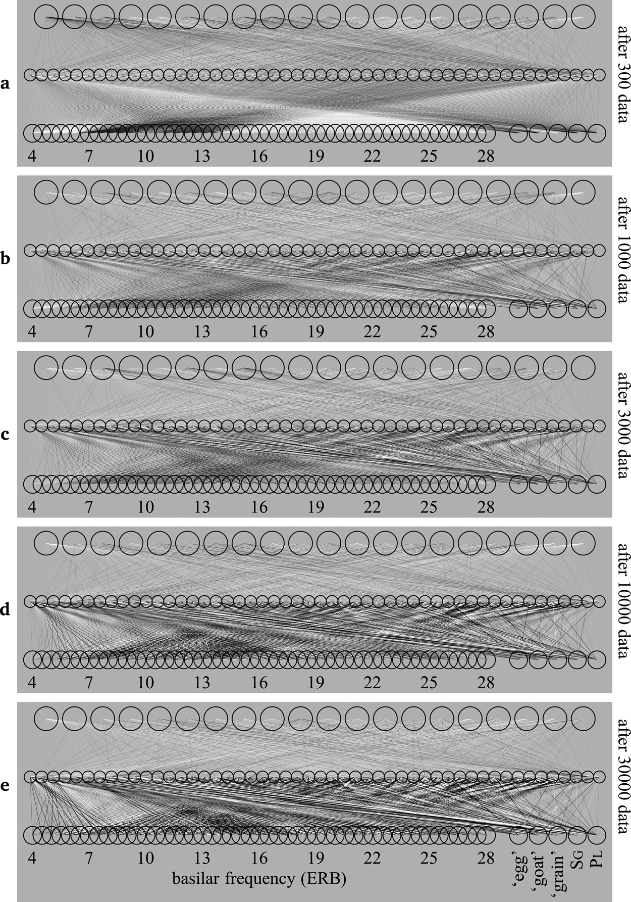
Utterances come in as vowel tokens, one at a time. When a vowel token comes in, the sound appears on the learner's sound level as in Figure 4, but without the utterance label a, e, i, o or u. We then go through the four phases of section 4: the middle and top levels start with zero activation, then activation spreads from the clamped sound level to the other levels, according to (1) and (3) repeated 10 times, then a learning step takes place according to (4) through (8), then the sound level is unclamped, allowing the activation to resonate stochastically according to (9), (10) and (11) ten times, and finally an unlearning step takes place according to (12) through (16). Figure 10 shows what the connection weights in the network look like after 300, 1000, 3000, 10000 and 30000 pieces of data. In comparison to the initial state of the network in Figure 9, each connection has become either excitatory or inhibitory.
The development of a network that is learning from a distribution of sounds.
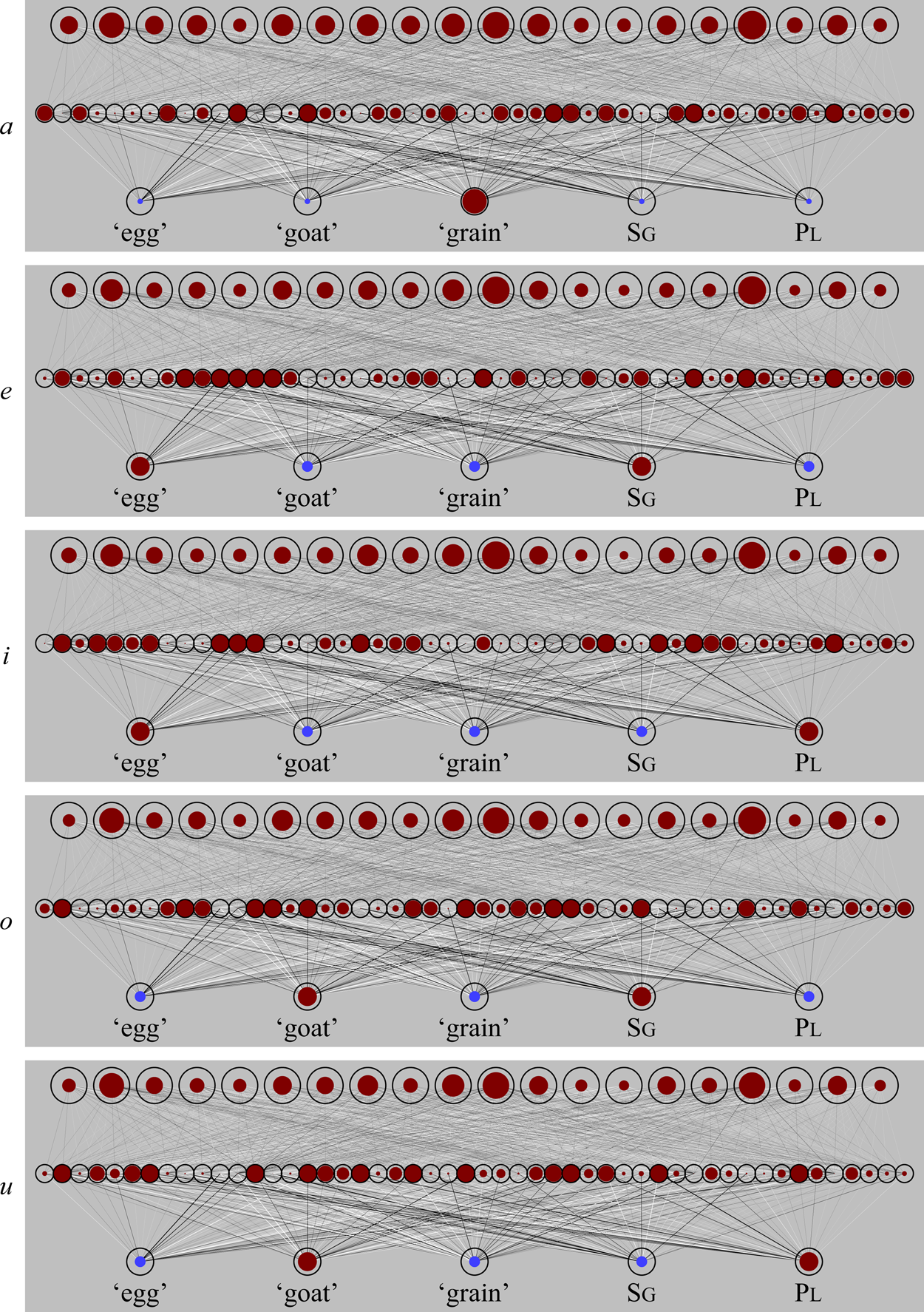
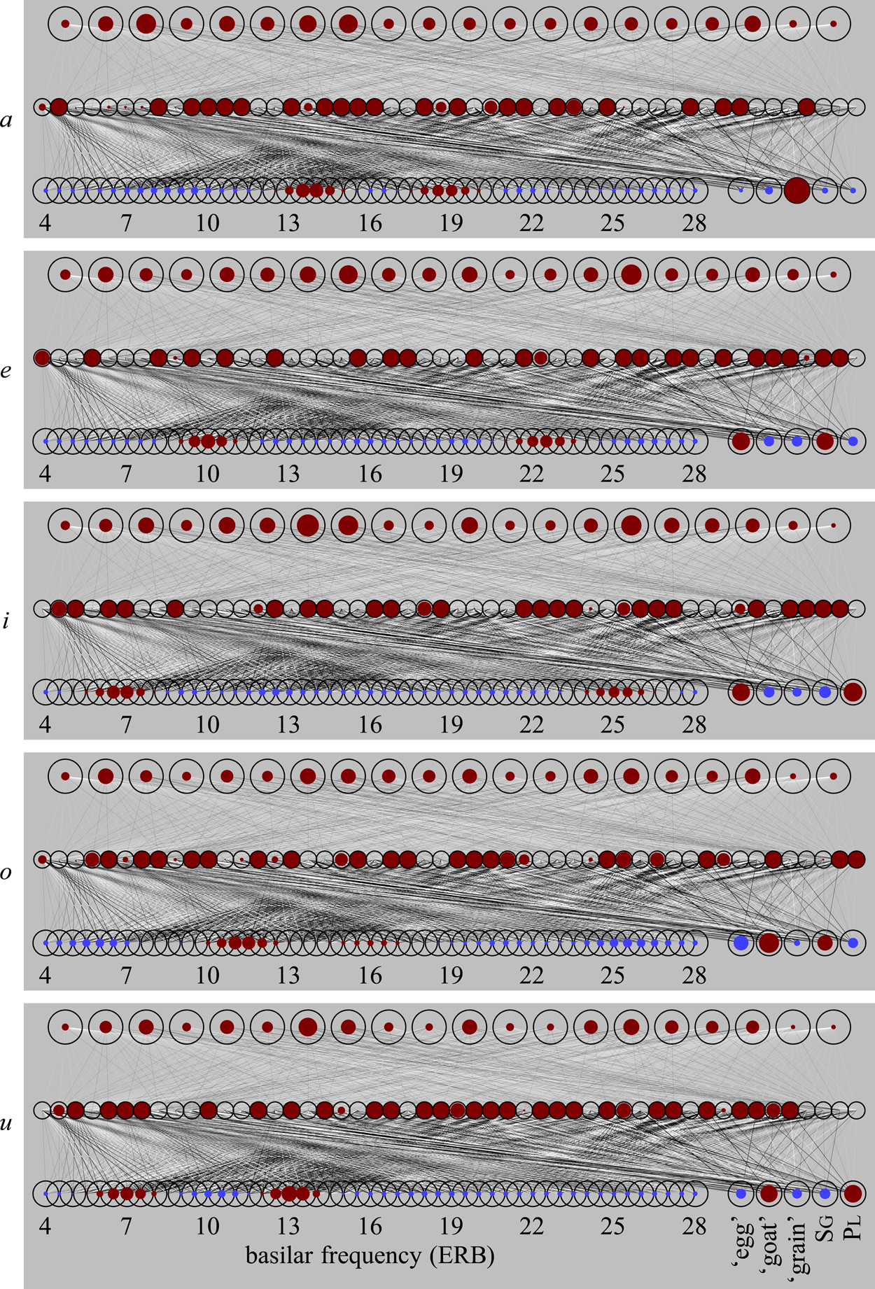
5.3 The resulting behaviour after sound-only learning: Categorization
The trained network is able to map incoming sounds to consistent patterns at the middle level. Figures 11a through 11u illustrate how the network, after having been trained with 10,000 sounds (i.e., Figure 10d), can classify typical instances of each of the five vowels. The tokens in Figure 11 were chosen completely randomly from the same normal distributions that the network had been trained on. The activities on the middle and top level are computed by repeating the spreading steps (1) and (3) ten times, while keeping the input constant (clamped).
The classification of five instances of an intended ambient a.
The classification of five instances of an intended ambient e.
The classification of five instances of an intended ambient i.
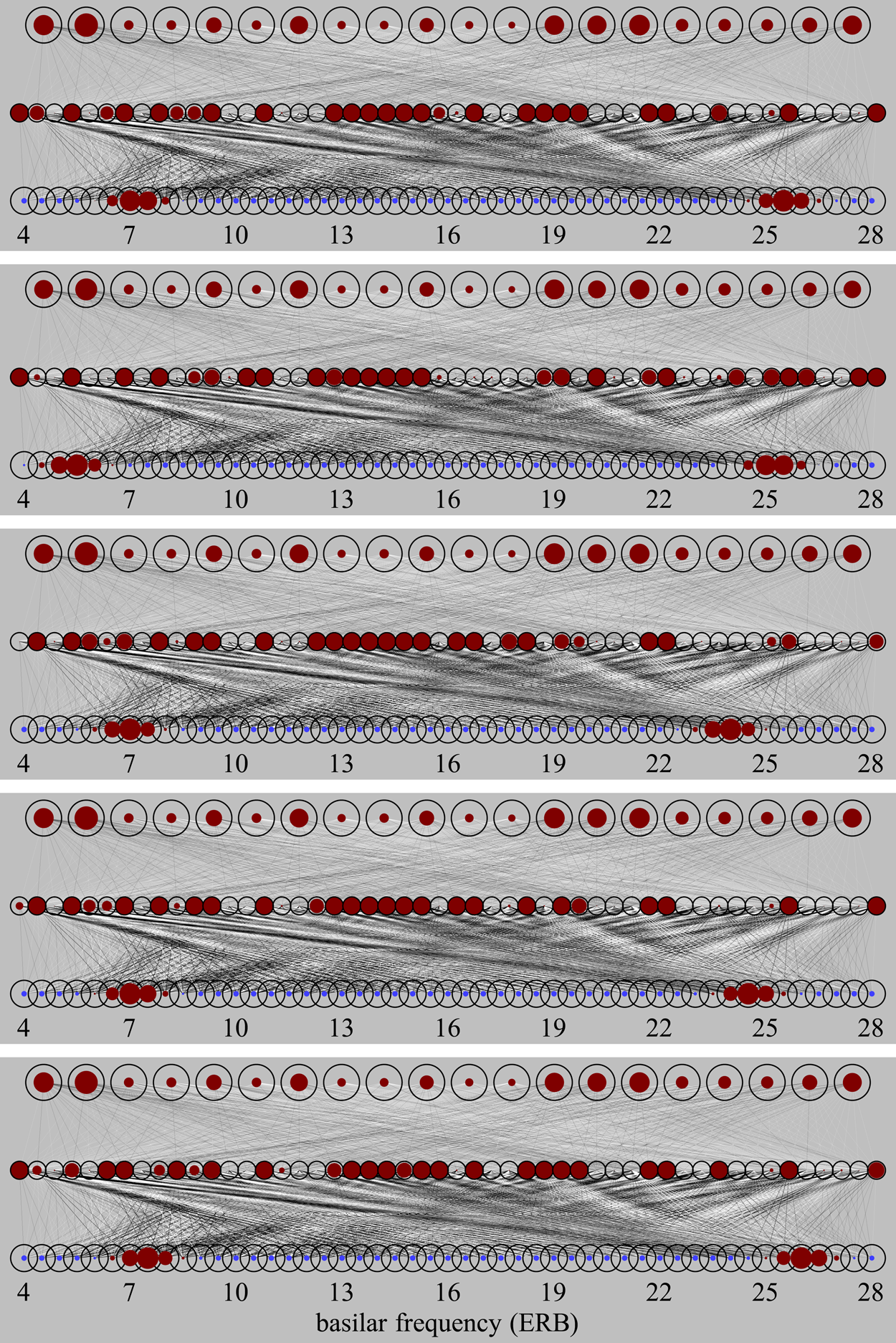
The classification of five instances of an intended ambient o.
The classification of five instances of an intended ambient u.
For each intended ambient utterance (a, e, i, o, and u), the relevant part of Figure 11 shows that the network classifies all five tokens in a slightly similar way, as measured by the activity patterns on the second level. We see some variation within each utterance (i.e., between the five tokens in a figure), which is caused by the randomness in F1 and F2, but the distinctions between the utterances seem to be greater.
The overarching question in the context of this study is what featural representations this network has formed at the phonological level. We answer this question in two stages: we first establish that the network exhibits categorical behaviour (a condicio sine qua non), and then study the presence and nature of featural representations.
5.4 A desirable emergent property of sound-only learning: Categorical behaviour
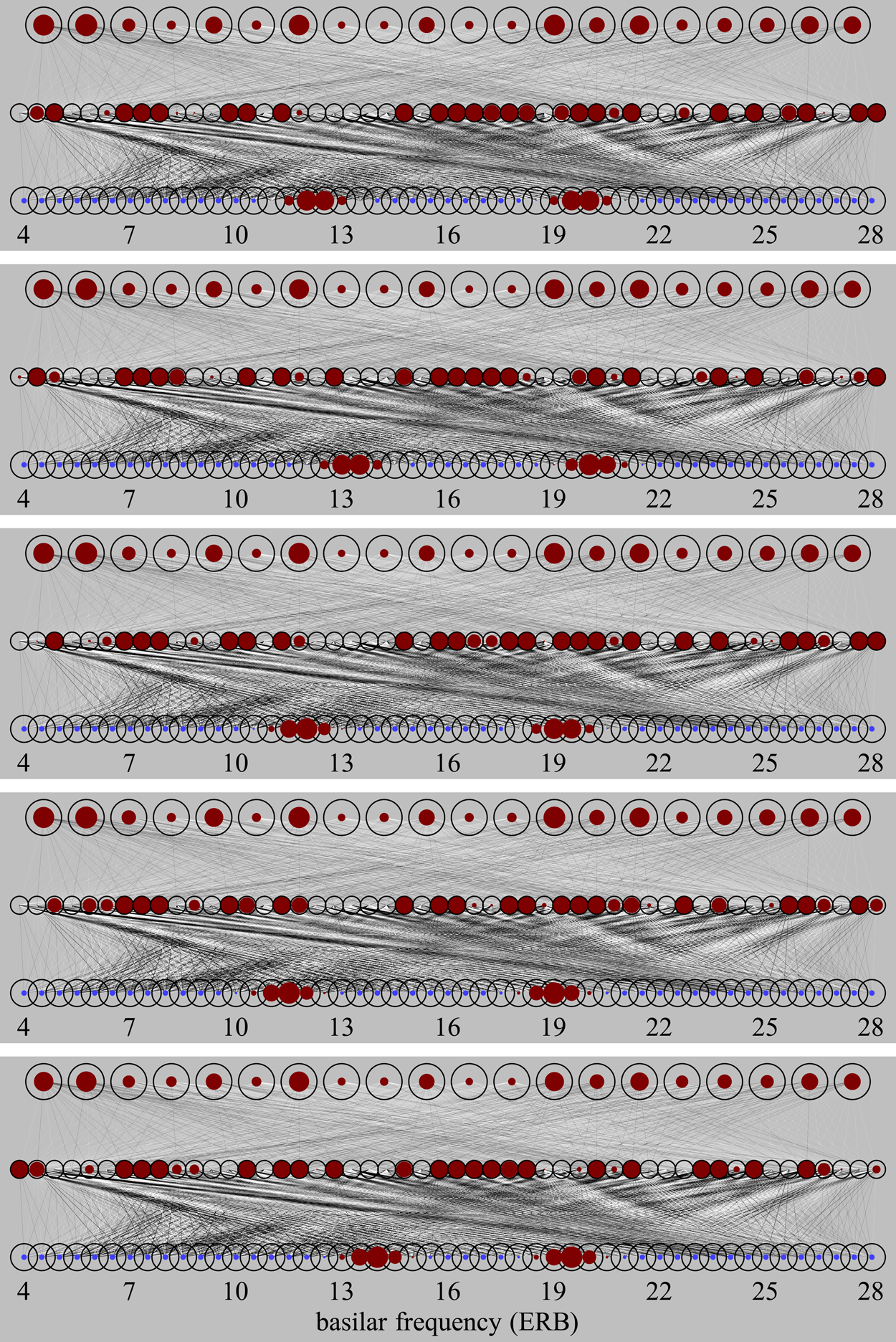
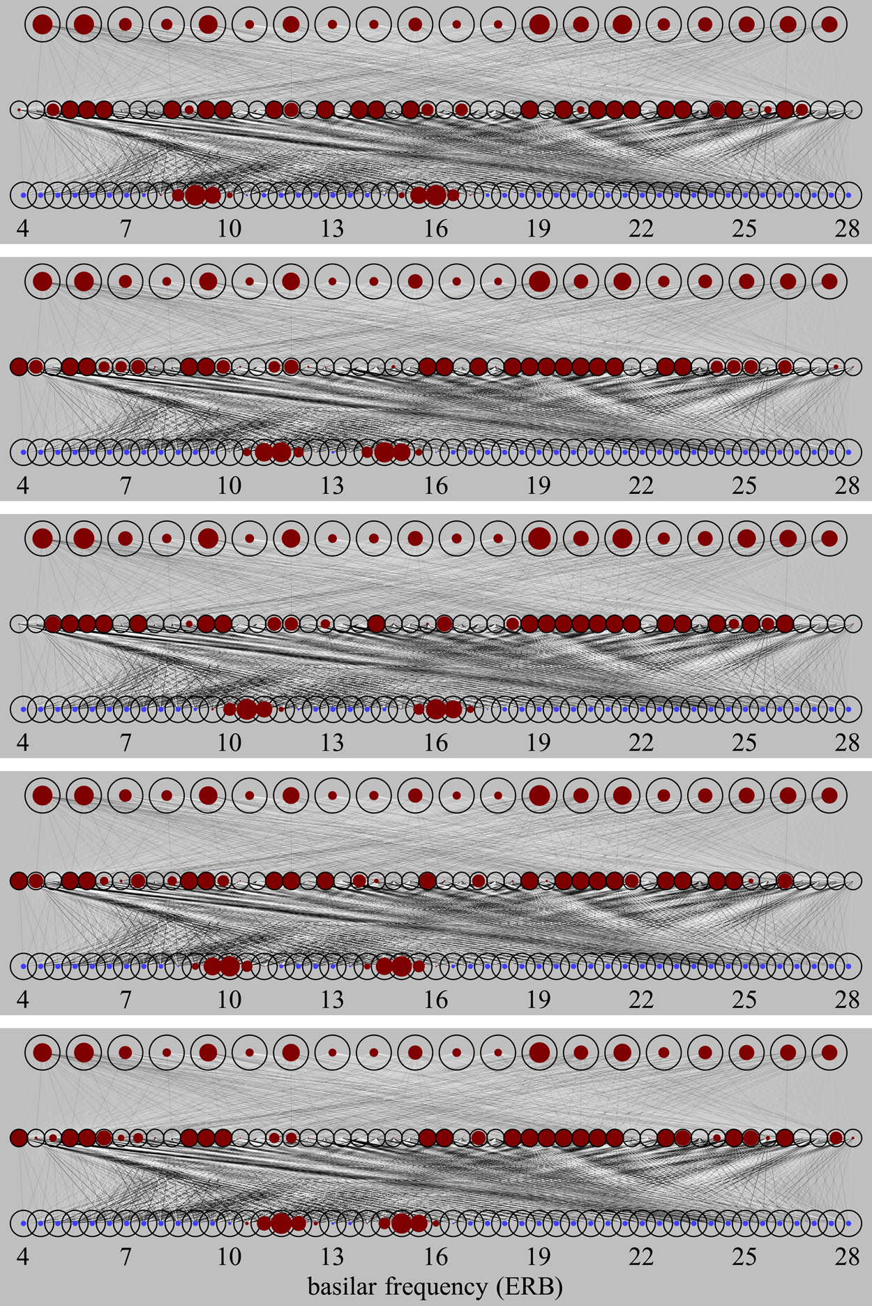
Categorical behaviour is measured by probing what the network “thinks” the applied sound was. Figure 12 again shows the network of Figure 10c, which has been trained with 3000 pieces of sound data. In Figure 12a, we apply a sound with an F1 of 14 ERB and an F2 of 18 ERB to the input, and we have this input spread to the middle level with (1), while the activity of the top level is still zero. In Figure 12b, we have subsequently applied an “echo”: activity spreads from the middle level not only to the top level according to (3), but also back to the bottom level according to (9), that is, the input is no longer clamped (held constant); the echo (or “resonance”) completes when activity has spread again from the bottom and top levels to the middle level according to (1). During this operation we see that the bottom level has changed: the centres of the bumps are no longer at 14 and 18 ERB, but just above 13 ERB and just below 19 ERB. We can repeat this echo procedure, that is, the sequence (3)–(9)–(1), several times, as in Figures 12cde, and ultimately the bumps on the bottom level end up being centred around 13 and 19 ERB, which are the two average formants for the utterance a. We can interpret this as follows: the network “thinks” that it has heard the utterance a.
The perceptual magnet effect at work, after 3000 sound data.
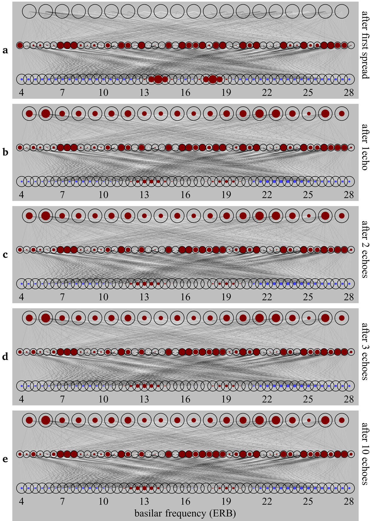
This auditory shift can be seen as an instance of the perceptual magnet effect: Kuhl (Reference Kuhl1991) found that human children in the lab would perceive instances of the vowel /i/ that lay some distance away from the most typical instance of /i/ as closer to the typical instance than they really were, and she visualized this as if those distant instances actually did lie closer to the prototypical /i/ than they were auditorily. In other words, the prototypical instance of /i/ seemed to serve as a “perceptual magnet” for the more distant instances. The perceptual magnet effect has enjoyed various earlier editions of computational modeling: Guenther and Gjaja (Reference Guenther and Gjaja1996) used neural maps, and Boersma et al. (Reference Boersma, Escudero and Hayes2003) used Optimality Theory, to create models where auditory space around the category centre would be shrunk at a level of representation above the incoming auditory level. By contrast, both BiPhon-NN with inoutstar learning (Boersma et al. Reference Boersma, Benders and Seinhorst2020) and the present simulations show the most literal version of Kuhl's hypothesis: the resonances in the network actually cause the incoming auditory representation itself to change in the direction of the category centre.
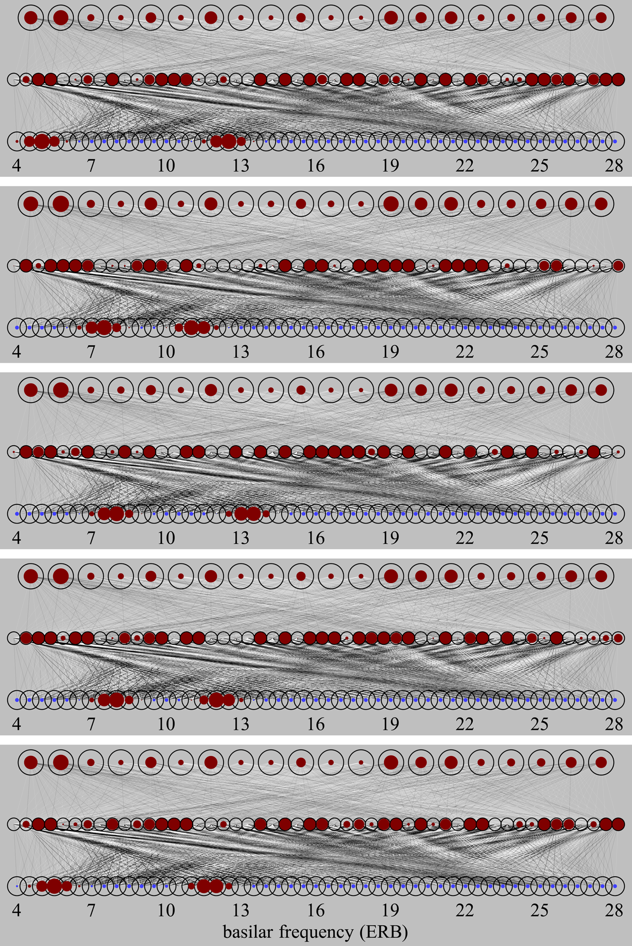
We can see in Figure 12 that the echo from the network to the input level is weak, but that it does exhibit the perceptual magnet effect. However, the perceptual magnet effect largely disappears with further learning: after having been trained with 10,000 sounds, as shown in Figure 13 (which is the same network as in Figure 10d), the network responds to an input of 14 and 18 ERB with a strong activity on the input level after multiple echoes, but the peaks ultimately appear around 14 and 18 ERB, replicating the input faithfully instead of moving toward the a prototype of 13 and 19 ERB. We will see in section 7.3, however, that the inclusion of meaning into the model will be able to maintain categorical behaviour.
Loss of the perceptual magnet effect, after 10,000 sound data.
Thus, while the goal of our network is just to be able to comprehend speech, a side effect of learning to comprehend speech is the emergence of perceptual magnets and discrete categories, from highly variable continuous phonetic input, just as in real human learners. To see how strongly the middle level has discretized the sound input, consider how the dimensionality of sound develops throughout the path from speaker to listener. The adult speaker produces two formant values, selected from anywhere in a two-dimensional space. We encode those two dimensions not on two input nodes (as Guenther and Gjaja Reference Guenther and Gjaja1996 did), but a bit more realistically on 49 nodes on our virtual basilar membrane, that is, as a 49-dimensional vector of activities. Because of the variation in formant values, formant centres can lie anywhere on the 49 nodes (and in fact in between nodes as well). The interaction with level 2 then reduces this dimensionality effectively to seven, as in the echo only seven locations along the virtual membrane can be formant centres (the perceptual magnet effect). In other words, level 2 acts as a big discretizer (already visible in section 5.3), roughly moving the dimensionality down from 49 to 7, although it consists of 50 nodes and could easily represent all 49-dimensional detail, but it has “decided” not to do so.
5.5 Featural behaviour after sound-only learning is sound-based
Now that the necessary requirement of discrete categorical behaviour has been established, we can start answering the central research question: how featural has our network become? That is, assuming that representations are discrete, how featural is the behaviour of these discrete representations? We measure this by measuring the similarity of the five “standard” (= average) utterances, which are defined in Table 1, to each other.
Phonological similarity should be measured at the level that is most likely to be “phonological”. As the top level (see Figure 12) makes little difference between the utterances, we decide to measure the phonological similarity between two utterances as the similarity of the two patterns generated at the middle level. To generate a pattern in the network, we apply the sound of the utterance to the bottom level, after which we can choose from two ways to spread this input activity up: with the input clamped, or with the input unclamped. Keeping the input clamped (i.e., fixed) entails that we spread the input activity up in the network according to the first phase of section 4, that is, a tenfold sequence of (1) and (3). This is identical to what we did for Figure 11. Letting the input unclamped (i.e., free to change), entails that the input activity resonates throughout the network, via repeating (1), (3) and (9) 10 times; this includes changes at the bottom level, as was also done in Figures 12 and 13. The unclamped version may be the more realistic situation of the two, although one can also argue for a combination (e.g., an incoming sound may stay in sensory memory for a while, but not throughout processing). We found that the results hardly depend on the choice between these three options; in the tables below, we therefore show the pattern similarities only for unclamped input.
The similarity between two middle-level patterns A and B is computed as their cosine similarity, which is the inner product of patterns A and B, divided by the Euclidean norm of pattern A and by the Euclidean norm of pattern B. The result is a value between 0 (minimal similarity) and 1 (maximal similarity); the tables show these values as percentages.
Table 4 shows the similarities between each pair of possible utterances, after applying the corresponding standard formant values of Table 3, for the learner depicted in Figures 10, 11, 12 and 13. High similarities are marked in green (or with dark shading).
Phonological similarities between the standard forms of the five utterances in comprehension after sound-only learning (in percent)

If we repeat this simulation for a different learner, the result will be slightly different, because the order of presentation of the data is random and because the Bernoulli step in unlearning is random. Table 5 therefore shows the average result of 100 different virtual learners.
Phonological similarities between the standard forms of the five utterances in comprehension after sound-only learnings, averaged over 100 learners (in percent)

Table 5 shows that after learning from sound alone, the deep representation of the utterance e is similar (74.7%) to that of o. The cause must be that these two utterances come with identical F1 values.Footnote 7 Likewise, the representation of i has become similar to that of u (72.5%), by the same cause. Curiously but perhaps unsurprisingly, the representation of a is similar to that of u (71.5%). The cause must be that the average F1 of a equaled the average F2 of u in the input.
In phonological theory, similarity between phonological representations can be expressed as the number of features that they share. Thus, /p/ and /a/ are very dissimilar, because they differ in many features (consonantal, labial, low, sonorant, voiced…), whereas /p/ and /b/ are very similar, because they differ only in one feature (voiced). In our network we have an analogous situation; the fact that the activity patterns of e and o at the middle level are similar (74.7%) means that there is a good chance that if a certain node is active for e, it will also be active for o. These shared nodes, then, correspond to what phonological theory calls shared features: if two cortical representations are similar, this means that these representations can lead to similar behaviour, which is precisely the criterion by which phonological features are defined. What Table 5 shows for e and o, then, is their feature sharing: the cosine similarity is the distributed counterpart of what phonological theory has hitherto been regarding as identical values for discrete features. For instance, /e/ and /o/ are thought in phonological theory as sharing the feature values /–low/ and /–high/ (discrete version), whereas in our simulations the two vowels [e] and [o] lead to shared activities on the middle level (distributed version). We therefore interpret the three high numbers in Table 5 as telling us that e and o share a feature, that i and u share a feature, and that a and u share a feature.
As in Boersma et al. (Reference Boersma, Benders and Seinhorst2020), the emergence of an appropriate number of categories for the target language is due to our choice to work within a distributed regime: while for establishing, for instance, seven features (i.e., our three shared ones, and perhaps three to five unshared ones) one would need only seven nodes at the middle level, it is important that such a number of features (i.e., attractors of discrete behaviour) have emerged in our case even if the middle level has an abundance of 50 nodes. A single brain structure with a large number of nodes allows for the number of emergent categories to vary with the properties of the language that the brain happens to be learning; this is a desirable property of a type of network that should ultimately be able to simulate the acquisition of any (and all) of the languages of the world.
5.6 Interpretation of the sound-based features
We conclude that the middle level of the network, after having been trained with 10,000 sounds, contains evidence for three features. What should we call these features? As a phonologist you would be eager to say that the feature that connects the utterance e with the utterance o is a height feature, with the value /mid/ if you believe in ternary features, or with the value combination /–high, –low/ if you believe in binary features. This is because similar behaviour of /e/ and /o/ has been observed in so many languages that phonologists have come up with a name for it, and it is a name that is mnemonic for an articulatory gesture (jaw height, which uses the same muscles for [e] and [o]) or a body phenomenon (tongue height, which uses different muscles for [e] and [o]). This name is vowel height. The second feature, shared by i and u, could be labelled /high/ or /+high/ or /+high, –low/, and is another instance of what phonologists would call vowel height. The third feature that our network created is based on an identical spectral peak (on the basilar membrane) for a and u. As a phonologist you would not easily come up with a name for this feature, perhaps because a similar feature has not been observed much in the languages of the world, so let's arbitrarily call this feature /gamma/. From the standpoint of the network, however, the three features have an equivalent status: they have all emerged from incoming sounds, and no innate or universal labels were necessary or indeed possible. We would like to say that all three features have been created in an equally arbitrary way on the basis of auditory similarities that the utterances of the language happen to possess. The features are linked to phonetic content, but do not contain phonetic content themselves.
Now that we have seen that sound-only learning led to the emergence of three auditory-based features, each corresponding to a spectral peak that is used in two of the five utterances, we are prepared for identifying which of the features that will emerge from sound–meaning learning in section 7 are phonetically based.
6. Learning from meaning alone
Our second set of simulations establishes what happens if a learner confronted with our toy language has access only to the meanings, and not to any sounds.
6.1 The network before and after learning
For learning from meaning alone, we use the network in Figure 14, where the input level consists of morphemic nodes only.
Initial state of learning from meaning alone.
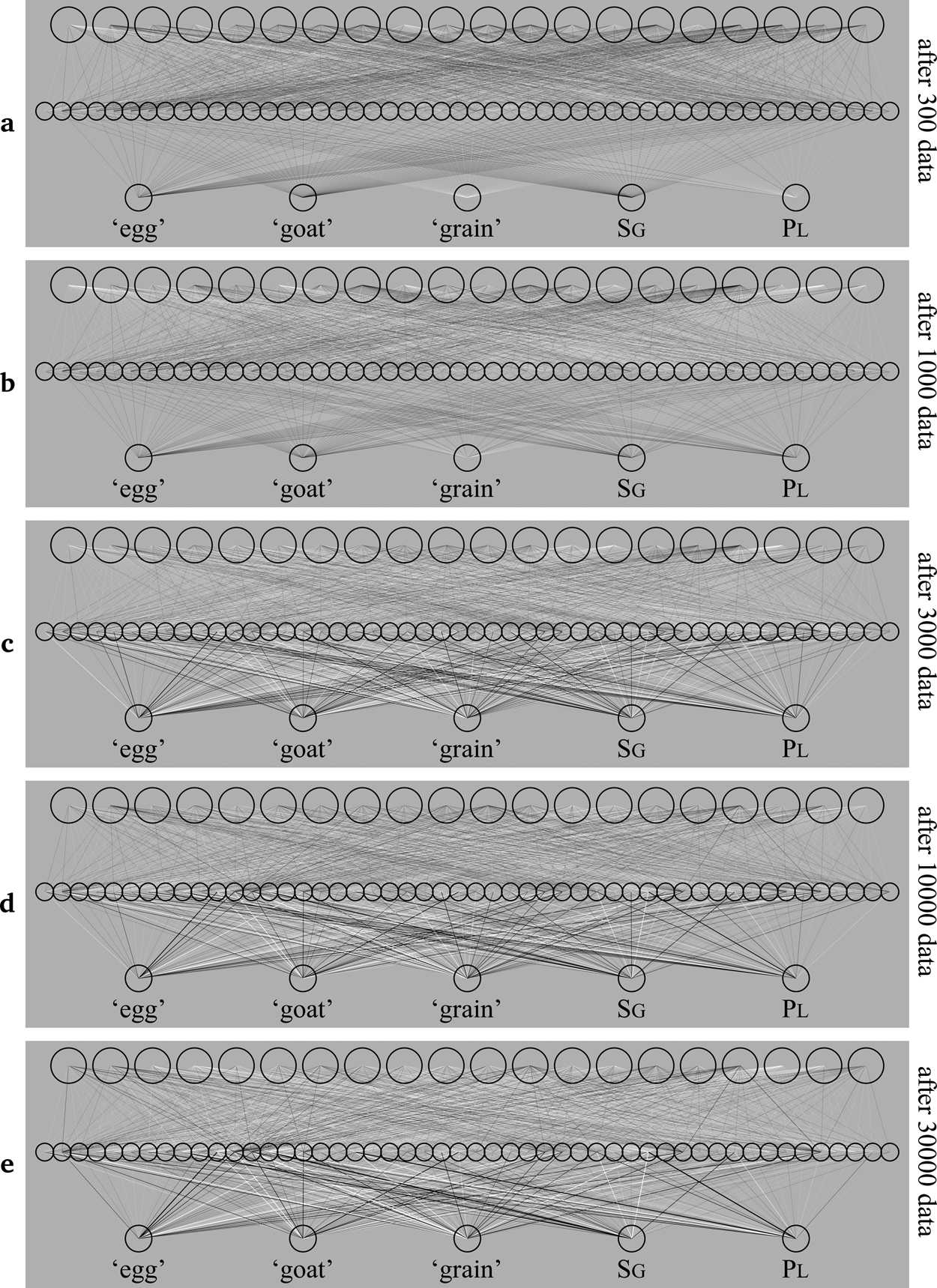
Following this initial state, we apply 10,000 meanings. For each meaning, we choose an utterance from the five possible ones, each with 20 percent probability, and perform a learning step by going through the four learning phases of section 4. After the 10,000 learning steps we arrive at the network in Figure 15d. Figure 15 also shows the network at several other stages of maturity.
The development of a network that is learning from meaning alone.
6.2 The resulting behaviour after meaning-only learning
In Figure 16 we can see that each of the five composite meanings causes a different pattern at the middle level.
Meaning-only production of the utterances a, e, i, o and u.
6.3 Featural behaviour after meaning-only learning is meaning-based
The learner of Figures 15 and 16 gives the phonological similarities in Table 6. Each of the cells in this table has been computed in the usual way (also seen in section 5.5): apply the utterance of the row to the input level and have the network cycle ten times through (1), (3) and (9), doing the same for the utterance of the column, and computing the cosine similarity between the two 50-dimensional vectors that result at the middle level.
Phonological similarities between the five utterances in production after meaning-only learning (in percent)

As every learner receives the meanings in a different order and undergoes different samples of the Bernoulli deviate, it is again useful to look at what 100 learners do. Their average phonological similarities are in Table 7.
Phonological similarities between the five utterances in production after meaning-only learning, averaged over 100 learners (in percent)

Our single learner or our 100 learners, with freely changing input levels, all end up the same. Thus, e is similar to i (72.6%), apparently because e and i share the stem that means ‘egg’. Likewise, o is similar to u (72.7%) because they share the partial atomic meaning ‘goat’. Also, e is similar to o (72.7%), apparently because e and o share the grammatical morpheme sg. Likewise, i is similar to u (72.6%) because they share the partial atomic meaning pl.Footnote 8
6.4 Interpretation of the meaning-based features
Just as with the sound-only learning of section 5, the high similarity between e and o (72.7%), and therefore the similarity of their phonological and extra-phonological behaviour, will be ascribed by phonologists to the influence of a height feature such as /mid/ or /–high, –low/. Likewise, the high similarity between i and u (72.6%) will be ascribed to the feature value /+high/ or so.
However, e is also very similar to i (72.6%). A phonologist would ascribe this to the feature /front/ or /–back/, suggesting an articulatory provenance. From the auditory point of view, however, our toy language shows no evidence for this feature: articulation is not included in the model, and e's F2 of 22 ERB is not more similar to i's F2 of 25 ERB than for instance e's F1 of 10 ERB is from i's F1 of 7 ERB; if a difference of 3 ERB is not enough to warrant the same feature value in the latter case, then it should also fail to yield the same feature value in the former case. What we witness here is that a morphological alternation causes the emergence of a feature, and that a phonologist can be biased enough (from experience with processes in other languages, or from knowledge of articulation) to describe this morphology-based contrast with the use of a phonetic label for which there is no direct evidence. At this point we expect many readers to object, saying that the backness feature does have phonetic support. Of course it does so in general, but it does not do so in the small world of our toy language, and still the feature has emerged substance-freely from the morphology. See section 8.4 for more discussion, with normal phonological examples to underline the point.
7. Learning from sound and meaning jointly
Now that we have seen what features arise if we train the network with sound only (section 5) and with meaning only (section 6), we can investigate what features arise if we train the network with sound and meaning together, and identify which of these features appear to come from the sound, and which from the meaning. The goal of the network is to produce and comprehend speech in a manner appropriate for our toy language, while the goal of our investigation is to identify and interpret the hidden representations that happen to emerge while the network is working toward its goal.
7.1 The network before and after learning
The network architecture, then, is as in Figure 17. Sound and meaning together form the input level at the bottom. This architecture is different from that of Chládková (Reference Chládková2014) and our Figure 1, where sound sits at the bottom and meaning at the top. This side-by-side input configuration is typical of Deep Boltzmann Machines and of the content-addressable memories by Kohonen (Reference Kohonen1984). The idea is that if sound and meaning are trained together as one input, then applying only a partial input (e.g., a sound only) should elicit the complete input that this partial input had been a part of during training (the whole input has been “content-addressed” by a part of the input). In our case, applying only a sound to the input (after training) should make the network retrieve the remainder of the input, which is the meaning that the sound had been paired with during training, and, conversely, applying a meaning to the input should make the network retrieve the sound that that meaning had been paired with during training (this “completion task” is also what Smolensky Reference Smolensky, Rumelhart and McClelland1986: 206 suggests using Restricted Boltzmann Machines for).
Initial state of learning from both sound and meaning.
Training, then, consists of applying, in sequence, 10,000 sound–meaning pairs to the whole input level of 54 nodes. For each sound–meaning pair, one of the five possible utterances is randomly chosen with 20 percent probability, the sound input representation is computed by Table 3 for that utterance with the appropriate variation of Figure 2 (as in section 5), and the meaning nodes are set as in Table 1 for that utterance (as in section 6). It is crucial that the sound and the meaning are derived from the same intended utterance. Thus, if the intended utterance is e, the 49 sound nodes will receive bumps in the vicinity of 10 and 22 ERB, and the ‘egg’ and sg nodes will switch on. After the input level has been filled in this way, the network goes through the learning phases of section 4. After having seen the 10,000 sound–meaning pairs and having gone through the four learning phases for each of these pairs, the network's wiring ends up as in Figure 18d. Figure 18 also shows earlier and later stages in the acquisition by our virtual learner.
The development of a network that is learning from both sound and meaning.
7.2 Behaviour of the trained network: production
A required property of the trained network is that when we apply a meaning to the input while setting the input sound to zero, the network is able to produce an appropriate sound.
There are several ways to map meaning to sound. One method could be to apply a meaning to the five meaning input nodes (setting the 49 sound input nodes to zero) and spread the activity up using (1) and (3) ten times, and after that applying (9), (10) and (11) ten times. In this case, we would be mimicking the learning procedure, but without changing the weights and biases; the second half of the procedure would be responsible for computing a sound, and would also potentially modify the meaning. Another method could be to maximize the clamping of meaning: apply a meaning to the five meaning input nodes (setting the 49 sound input nodes to zero) and spread the activity throughout the network using (1), (3) and (9) ten times, but keeping the five meaning input nodes fixed. In this case, the sound level would be influenced from the first application of (9) on, and the meaning level would never change. A third method is what we use: we apply meaning to the five meaning input nodes once (setting the 49 sound input nodes to zero) and immediately cycle through (1), (3) and (9). This means that the sound level is influenced from the start, and the meaning level is allowed to change from the start, as well. We have tried all three methods, and they give very similar results when it comes to measuring the similarity tables, and hence in the features that the network comes up with. Our reason for presenting only the third option here, namely unclamping the whole input from the start, is a) that it is simple and b) that it is the most challenging and informative. The method is the most challenging because it must have the largest chance of wandering off into a different meaning, since the meaning has been applied only at the very beginning of activity spreading; thus, if we get consistent results even when unclamping from the start, we will have shown that the model is robust. The method is the most informative because the figures will show not just the applied intended meaning, but the meaning that the network ends up thinking the speaker has intended.
Figure 19, then, shows the production of the five utterances. We see that the sound level typically comes to display two bumps, and that these correspond to the average two formants for each of the five utterances. Thus, for utterance e we applied activity to ‘egg’ and sg at the beginning, and the network came up with bumps near 10 and 22 ERB, as is appropriate for e according to Table 3.Footnote 9
Production of the utterances a, e, i, o and u.
The sound produced by the network for Figure 19 for a specific utterance is always the same, because sequences of (1), (3) and (9) are deterministic. It is interesting to see whether the stochastic version of production, that is, using a tenfold repetition of (10), (11) and (9) instead,Footnote 10 leads to realistic variation in the sound. Figure 20 shows this for the utterance a ‘grain’. We indeed see variation of the type that can be expected for formant values. We deliberately chose to include a rare instance (the second from above) in which the initially applied meaning was almost overruled by the network (because of the randomly low F1, the meaning ‘sg’ became as strong as ‘grain’). The kind of overruling is a peril of letting the input run free; in real linguistic processing this might correspond to the phenomenon of “ineffability” (for OT: Legendre et al. Reference Legendre, Smolensky, Wilson, Barbosa, Fox, Hagstrom, McGinnis and Pesetsky1998), where a morpheme is erased from the input because the network decides that it cannot be pronounced (or conversely, if a sound is erased from the input because the network decides that it cannot be interpreted). We do not pursue including the Bernoulli noise any further here; suffice it to say that it does not influence our results qualitatively.
Variable production of the utterance a, caused by Bernoulli noise.
After 10 resonances with unclamped input for one speaker, we obtain Table 8, in which we see two strong similarities (marked in green or with dark shading), namely that between i and u and that between e and o. These are pairs whose members are combined by both a shared F1 (low and mid, respectively) and a shared number (plural and singular, respectively).
Phonological similarities between the five utterances in production after sound–meaning learning (in percent).

This is confirmed when we average over 100 learners, as in Table 9: the average similarity between i and u is 65.9%, and that between e and o is 66.7%. A second layer of similarities (marked in yellow or with bright shading) has now become visible, namely between a and u (55.1%), which share a spectral peak only (at 13 ERB), and between e and i (53.5%) as well as between o and u (57.1%), which share a lexical meaning only (‘egg’ and ‘goat’, respectively). Combining the evidence from the cells marked in green and yellow (or with dark and bright shading), we can conclude that “phonological” similarity in production can be obtained on the basis of phonetic or semantic similarity alone, but that this phonological similarity is stronger if there is phonetic and semantic similarity.
Phonological similarities between the five utterances in production after sound:meaning learning, averaged over 100 learners (in percent)

7.3 Behaviour of the trained network: comprehension
Figure 21 shows how applying a random auditory form of each of the utterances a, e, i, o and u to the auditory part of the input level of the bidirectionally trained network works its way toward the meaning part of the input (the whole input level is unclamped). We see that in all five cases, the appropriate meaning is activated. Thus, this network can not only speak the language (as section 7.2 showed) but also understand the language.
Comprehension of random tokens of the utterances a, e, i, o and u.
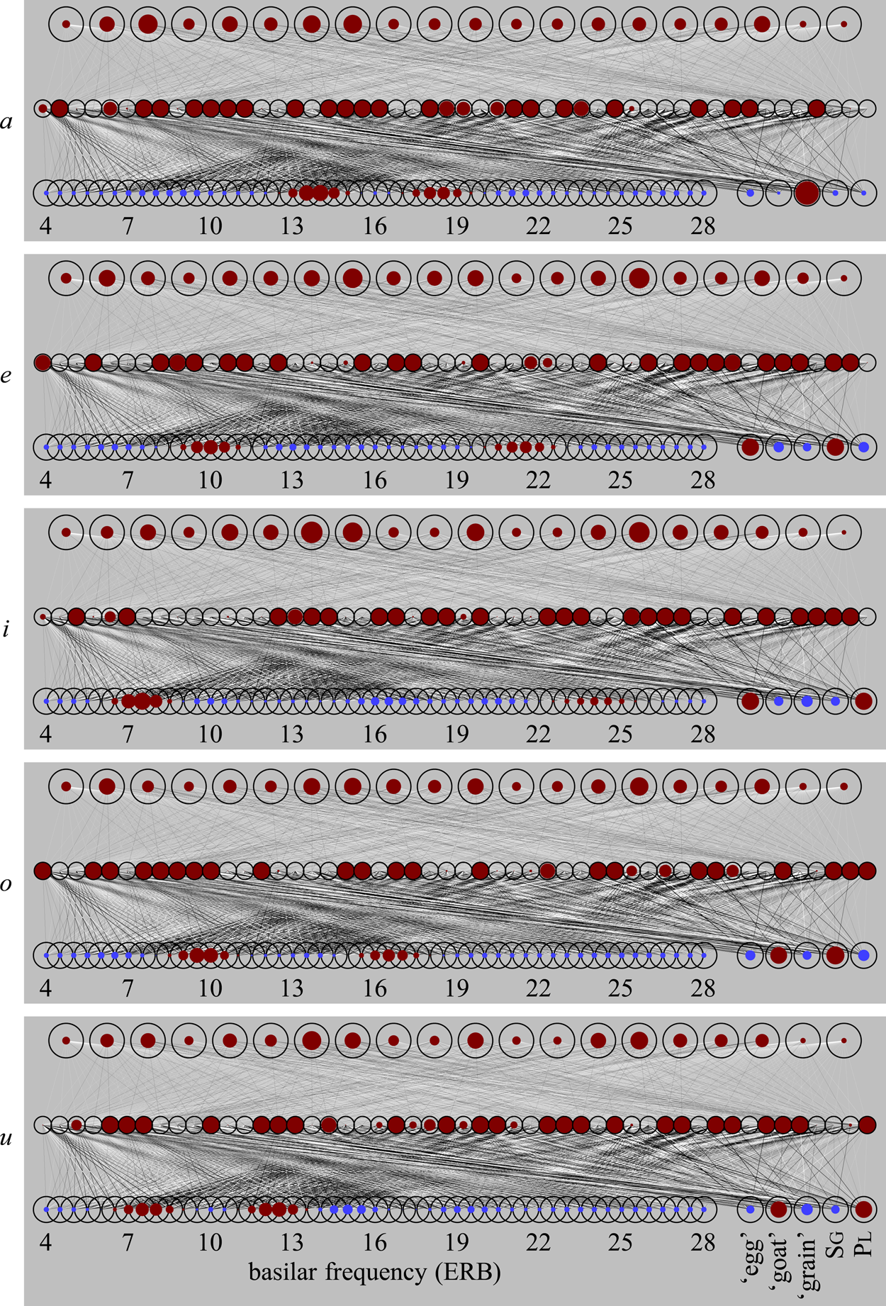
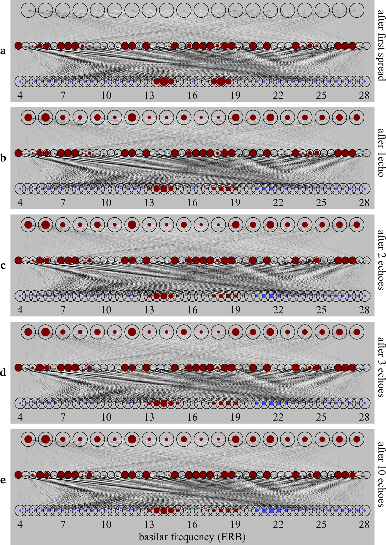
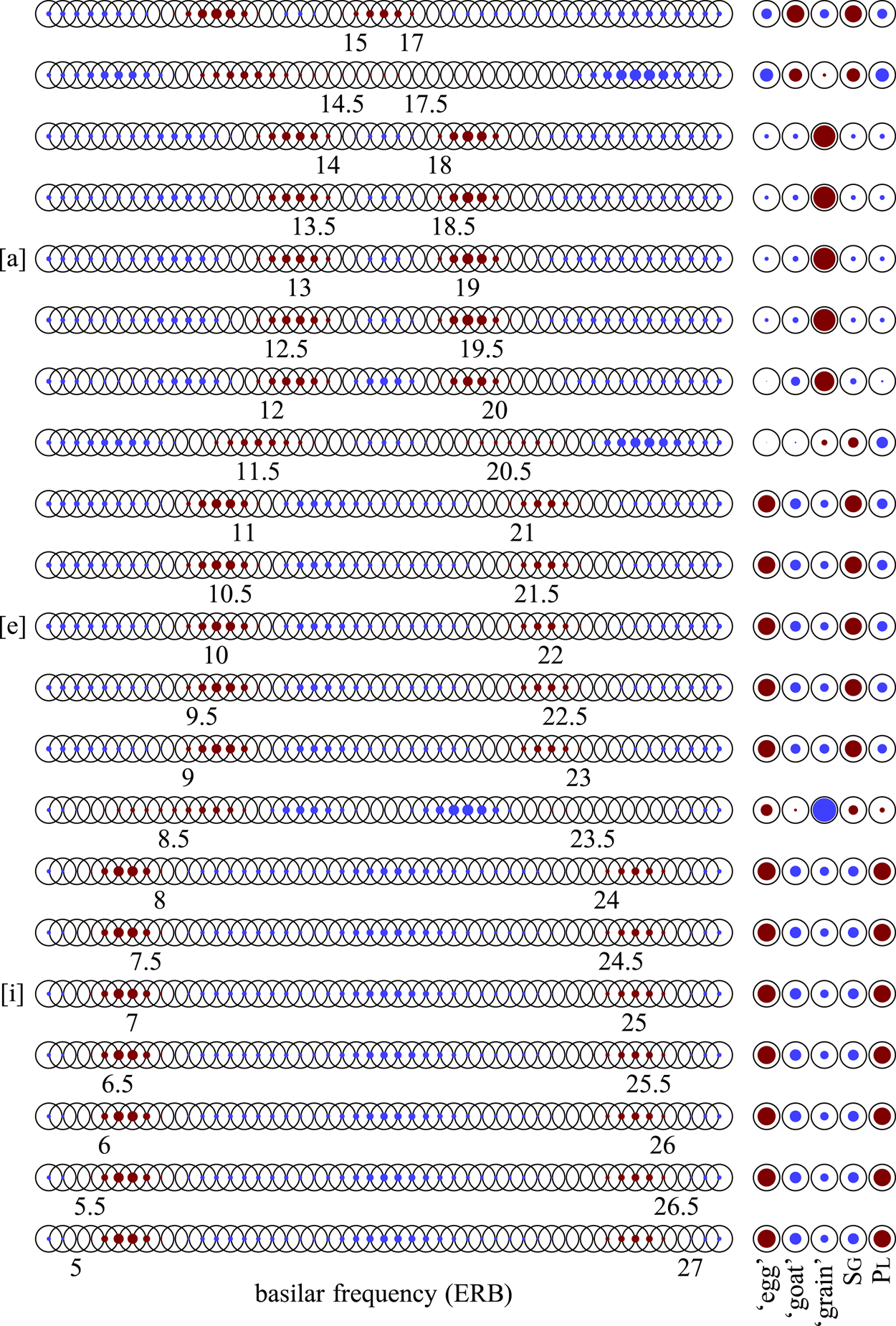
Figure 22 shows the perceptual magnet behaviour of the network. This figure is a level of abstraction higher than Figure 12, in which only one auditory input was applied and the change on the input level was measured after up to 10 echoes. In Figure 22 we show how the network (trained on 3000 data; i.e., this is the network of Figure 18c) changes 21 different auditory inputs, namely a continuum of front vowels from an F1 of 15 ERB and an F2 of 17 ERB to an F1 of 5 ERB and an F2 of 27 ERB, in 10 echoes. For instance, it can be seen that any of the five input vowels with an F1 between 9 and 11 ERB are interpreted by the network as actually having had an F1 of 10 ERB, which is the standard F1 of the e utterance. Perhaps more important, we see that the network comprehends all five of those vowels as ‘egg-sg’, and that it also classifies five other vowels as ‘grain’ and no fewer than seven vowels as ‘egg-pl’. All of these classifications are appropriate: comprehension is always done in the direction of the meaning whose average auditory correlate (i.e., auditory “prototype”) is closest to the given auditory input. This even goes for the extreme F1–F2 pair of 15 and 17 ERB, which just sounds like an F2 of 16 ERB with a missing F1, and therefore as the vowel [o], which should be comprehended as ‘goat-sg’, as it indeed is here (as a result, the corresponding F1 of 10 ERB is hallucinated in addition).
Scanning through the front vowels after learning from 3000 pieces of data: strong perceptual magnet effect and effective categorization.
As in section 5.4, the perceptual magnet effect gradually fades away with more training. For the network of Figure 18d, that is, after 10,000 learning data, the comprehension performance is as shown in Figure 23: the auditory input is now reflected somewhat more faithfully, with weaker perceptual magnetism than in Figure 22, but fortunately the classification behaviour is still fully appropriate for the language environment.
Scanning through the front vowels after learning from 10,000 pieces of data: the perceptual magnet effect has decreased, but semantic classification is still entirely appropriate.
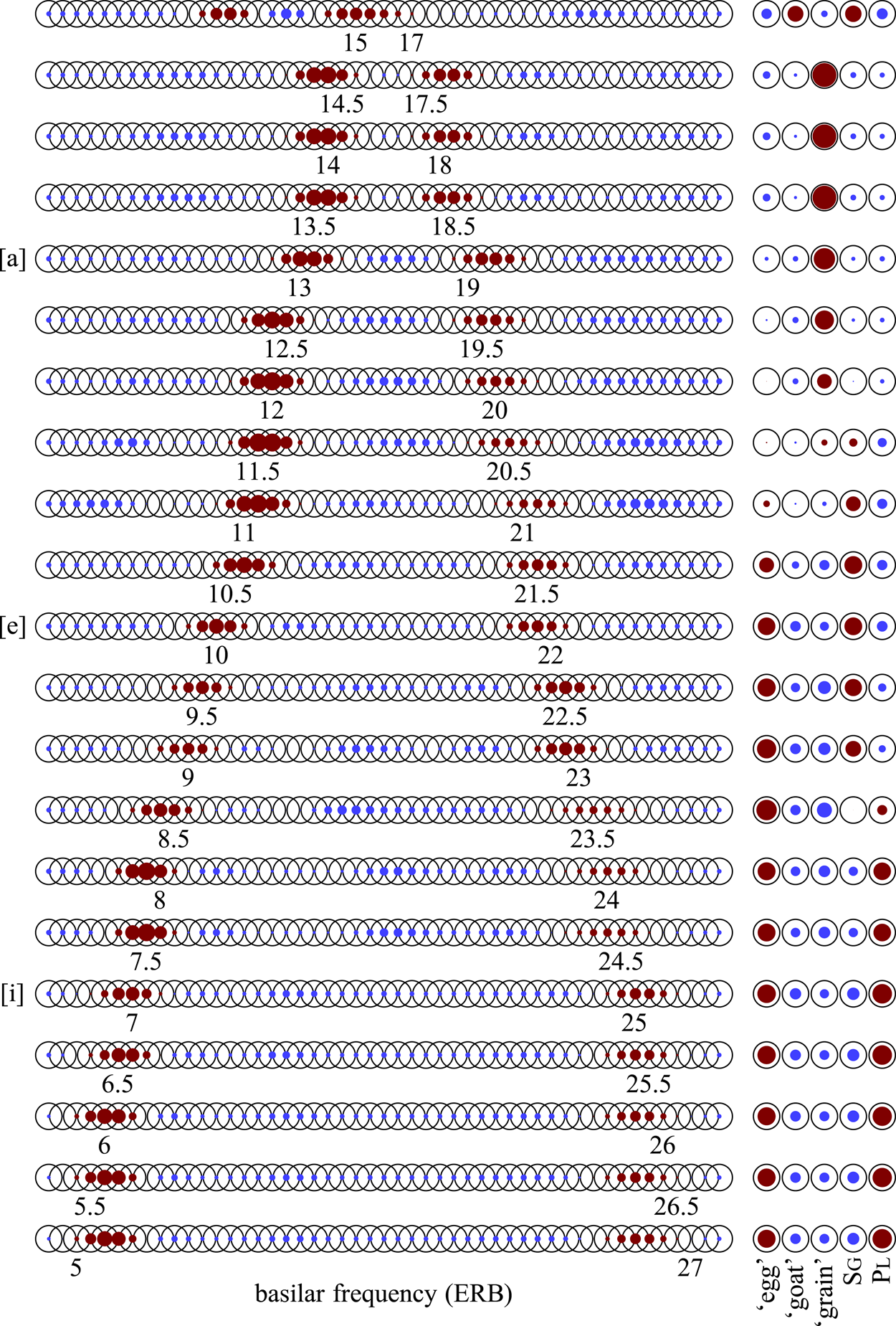
Having established that the network comprehends its target language well, and has done so via more or less discrete representations at the middle level, we can now have a look at the phonological representations that arise in comprehension. To determine the phonological similarity between the five utterances in comprehension, we compare what happens on the middle level when it is activated by the standard form of each utterance, that is, we apply the formant values of Table 3 to the auditory part of the input. Table 10, then, shows the similarities between the five standard utterances, for one learner (after 10,000 training data).
Phonological similarities between the standard forms of the five utterances in comprehension after sound–meaning learning (in percent)
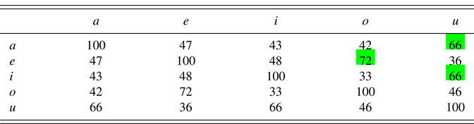
For the average learner in Table 11 we can tell a story similar to that for production in Table 9. The highest similarity is again found (in green or with dark shading) between the doubly matching i and u (67.2%) and between the doubly matching e and o (69.4%), followed (in yellow or with bright shading) by the auditorily-only matching a–u (61.8%) and then (in grey or with very dark shading) by the lexically matching e–i (47.9%) and o–u (47.7%). A fourth layer of similarities is found in the row of a, which as a mass noun has a “no-mismatch” with the numeric meanings of e, i and o. Finally, the lowest similarities are found when comparing e with u or o with i, pairs that clash on their lexical meaning as well as on their numeric meaning.
Phonological similarities between the standard forms of the five utterances in comprehension after sound–meaning learning, averaged over 100 learners (in percent)
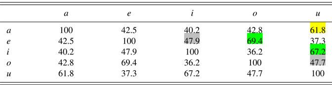
That we were able to tell the same story for Tables 9 and 11 indicates that it does not matter much whether our measured similarity is based on the production process or on the comprehension process. In both cases, the strongest featural behaviour appears between utterances that share both phonetic and semantic cues.
7.4 Changing the conditions: a related language
To test what happens if our network learns a language that is less “natural” than the one discussed throughout this article, Table 12 shows the featural results for the production of a language that anticorrelates sound and meaning: this language is like our usual toy language, except that singular and plural are reversed for one of the two count nouns: ‘goat’ is u (pronounced as [u]) and ‘goats’ is o (pronounced as [o]).
Phonological similarities between the five utterances in production after sound–meaning learning, averaged over 100 learners of an anti-correlating language (in percent)
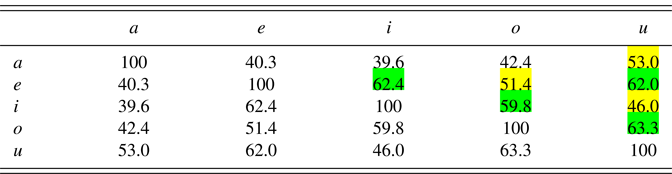
The strongest similarities (in green or with dark shading) are now wholly semantic: e and i share ‘egg’, e and u share sg, i and o share pl, and o and u share ‘goat’. The three phonetic similarities, no longer supported by morphophonological alternations, have been relegated to a second layer (in yellow or with bright shading).
Apparently, in our example, the semantics has stronger influence on the emergence of phonological features than the phonetics has. This could be caused by the fact that our auditory inputs are highly continuous and variable, whereas our semantic inputs are discrete and fixed; the effect might therefore go away once we model the semantics in a more variable way, as for instance in a more realistic setting where the real-world references of the utterances are ambiguous (Yu and Smith Reference Yu and Smith2007, McMurray et al. Reference McMurray, Horst, Toscano, Samuelson, Spencer, Thomas and McClelland2009). We therefore like to conclude only that in order to learn strong features from the phonetics, these features had better receive support from morphological alternations.
8. Discussion
We achieved our first goal, which was to devise an artificial neural network that can produce and comprehend our toy language. A side effect of learning to produce and comprehend speech was the emergence of discrete representations somewhere between the phonetics and the semantics, which we like to call “phonological features”. From this we can already conclude that modeling substance-free emergence with neural networks is feasible. This section aims to address our second goal, which was to identify the nature of the emerged features and to assess their suitability for the phonologist.
8.1 What features have emerged?
In our simulations, especially in the simulations with bidirectional input in section 7, phonological features emerged both bottom–up and top–down. In the bottom–up direction, we saw features emerge on the basis of phonetic similarities: one feature was shared by the utterances e and o on the basis of their shared average F1, another feature was shared by i and u on the basis of their shared average F1, and one feature was shared by a and u on the basis of the similarity between the F1 of a and the F2 of u. In the top–down direction, we saw features emerge on the basis of semantic similarities: one feature was shared between the utterances e and o on the basis of their shared singularity, one feature was shared between i and u on the basis of their shared plurality, one feature was shared between e and i on the basis of their sharing the ‘egg’ concept, and one feature was shared between o and u on the basis of their sharing the ‘goat’ concept.
The features that had both phonetic and semantic support, namely the one shared by e and o and the one shared by i and u, became the strongest. A possible interpretation of this fact in terms of phonological theory, which has no concept of feature strength, is a numerical one: e and o came to share two features, as did i and u, whereas the pairs a–u, e–i and o–u came to share a single feature each. Such an interpretation generalized to another toy language: we saw that depending on whether the semantic similarities between the utterances correlated or anti-correlated with the phonetic similarities, the phonetically-based features would be stronger or weaker, a fact that can again be explained by counting shared phonetic and/or semantic properties.
8.2 What phonological theories are compatible or incompatible with our results?
Our results seem to be compatible again with the grammar model of Bidirectional Phonology and Phonetics (BiPhon), whose larger structure is drawn in Figure 24 (Boersma Reference Boersma1998, Reference Boersma, Boersma and Hamann2009).
Grammar model of Bidirectional Phonology and Phonetics.
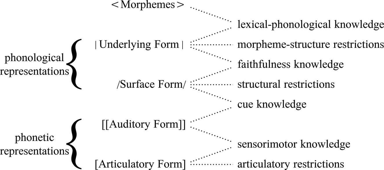
Figure 24 was originally designed for the Optimality-Theoretic version of the grammar model (BiPhon-OT), with the terms “knowledge” and “restrictions” both to be read as ‘constraints’. We can see the appropriateness of this model for the simulations of this article when comparing it with earlier versions of OT. Most phonologists study the mapping from Underlying Form to Surface Form (phonological production), which is why the creators of OT, Prince and Smolensky, as well as many followers, considered faithfulness constraints and structural constraints only. In such a restricted theory, phonetic influences on phonological choices would have to be implemented as structural constraints (e.g., *FrontRoundedVowel), and so it was done by many. However, with the phonetics represented outside phonology, as in BiPhon, no such intrusion of phonetics into phonology is necessary (Boersma Reference Boersma1998, Reference Boersma, Boersma and Hamann2009). Moreover, rigidly separating phonological from phonetics representations, as in Figure 24, allows us to also model the reverse process, namely comprehension (from Auditory Form to Morphemes; Boersma Reference Boersma1998, Reference Boersma, Boersma and Hamann2009 et seq.), as we also accomplished in the present article.
Figure 24 works not only within OT, but also for the neural-network version of BiPhon, (i.e., BiPhon-NN), with the terms “knowledge” and “restrictions” both now to be read as ‘connections’ (Boersma et al. Reference Boersma, Benders and Seinhorst2020). The present article is an especially simple instance of a computer simulation executed within BiPhon-NN.
Compatibility of our results with the BiPhon model cannot by itself corroborate the BiPhon model. To establish that, we also have to show that the simulations in this article are not theory-neutral, that is, that they are not compatible with many linguistic models. The results support the following three discriminative tenets of the BiPhon model:
-
1. Substance-freedom. Reiss (Reference Reiss, Hannahs and Bosch2017) gives as an example of substance-freedom that a grammar should just as easily represent a language with the common phenomenon of final devoicing as a language with the uncommon (or perhaps even unattested) phenomenon of final voicing. This was true of early generative phonology (Chomsky and Halle Reference Chomsky and Halle1968), where the rule [obs] → [–voi] / _$ had no formally preferred status over the rule [obs] → [+voi] / _$, but it was not true of early Optimality Theory, which proposed a universal markedness constraint *VoicedCoda to express the typological observation that codas tend to be voiceless rather than voiced. The BiPhon version of OT, on the other hand, has never worked with markedness constraints. It could have worked with structural constraints, but in that case it would have had both *VoicedCoda and *VoicelessCoda in its constraint set Con (probably next to *VoicedOnset and *VoicelessOnset and *NasalCoda and *VelarCoda and *AlveolarCoda and thousands of other never-heard-of ones), expressing no preference in Con for final devoicing over final voicing. The cross-linguistic preponderance of final devoicing would then come about as a preponderance of the ranking *VoicedCoda >> *VoicelessCoda, explained perhaps by phonetic influences during acquisition, but crucially not by a preference of the phonology itself. The phonetic influences could come from an articulatory constraint, but articulatory constraints perform their work on the Articulatory Form, not (or not directly, see below under 3) on the Phonological Surface Form.
-
2. Separation of levels. BiPhon-OT can actually explain phenomena like final devoicing with reference to cue constraints only, that is, constraints that link surface phonological structure to phonetic representations, keeping the phonological structure itself substance-free in the very strong sense of being devoid of structural constraints (Boersma and Hamann Reference Boersma, Hamann, Calabrese and Leo Wetzels2009: section 7.1).Footnote 11 More generally, the fact that BiPhon-OT can successfully make a separation between what is phonological and what is phonetic is caused by its multiplicity of levels of representation, that is, phonological levels are separate from phonetic levels; they are linked, but not intertwined or identical. In BiPhon-NN, the levels that presumably contain structure (e.g., phonological features) are physically separate from the ones at which phonetic representations are applied; the relevant example from the present article is that we look for phonological features at the middle level, which is separate from the phonetic and semantic layers at the bottom.
-
3. Counterdirectional influences. In BiPhon-OT, articulatory considerations can influence phonological decisions in production, just as phonological considerations can influence morphological decisions (Boersma and Van Leussen Reference Boersma and Van Leussen2017). That is, there is bottom-up influence between levels in production, just as BiPhon-OT allows top-down influence in comprehension (Boersma Reference Boersma, Boersma and Hamann2009: section 7.1). This is not because representations are somehow intertwined or mixed (as they are in variations of the usual two-level OT that mix phonetically-inspired with structural-inspired constraints), but because they interact at their interfaces, so that information flows both up and down through the levels. In BiPhon-OT this is implemented as parallel evaluation across multiple levels (as in Boersma and Van Leussen Reference Boersma and Van Leussen2017), while in BiPhon-NN (i.e., the present article) this is implemented by having multiple rounds of activity spreading (resonances) while the activities within the network are settling.
The combination of tenets 1 through 3 warrant the observation that the BiPhon-NN model espoused in the present article is indeed the neural-net counterpart of BiPhon-OT, and not of any other kinds of OT, which typically work with innate substance-full constraints, unseparated levels of representation, and (if the levels are separated) sequential levels (e.g., Bermúdez-Otero Reference Bermúdez-Otero1999). The findings of the present article (substance-freedom through emerged linking, separation of levels through the success of the intermediate level in production and comprehension, and realistic perceptual magnetism through bidirectional settling) therefore corroborate BiPhon-NN and thereby many of the tenets of BiPhon-OT as well. We are aware that in this reasoning, some circularity remains until neural-net editions of other theories are available or until it has been shown that such cannot exist.
8.3 Where is our theory on the substance-freedom scale?
We think that the grammar model in Figure 24 is fully compatible with a substance-free view of phonology (Hale and Reiss Reference Hale, Reiss, Burton-Roberts, Carr and Docherty2000, Reference Hale and Reiss2008; Blaho Reference Blaho2007, Iosad Reference Iosad2013), in which phonological features and processes make no reference to phonetic substance. We also think that the model is quite opposite to the substance-full theories of phonology proposed by Browman and Goldstein (Reference Browman and Goldstein1986) and Gafos (Reference Gafos2002), in which phonological representations are articulatory in nature, or by Flemming (Reference Flemming1995), in which phonological representations can be evaluated for their auditory correlates, or by Kirchner (Reference Kirchner1998), in which phonological representations can be evaluated for their articulatory correlates.
Not everybody agrees. In an overview of phonological theories, Zsiga (Reference Zsiga2020: 248) presents a continuum for how theories regard the role of phonetic markedness in phonology, ranging from (1) “phonology is not natural”, for which she cites Hjelmslev (Reference Hjelmslev1943), Anderson (Reference Anderson1981), and Hale and Reiss (Reference Hale and Reiss2008), (2) “pressures of markedness and naturalness play out in sound change, but should have no representation in synchronic phonology”, for which she cites Blevins (Reference Blevins2004), (3) “phonetically natural alternations are more easily learned” in acquisition, for which she cites Wilson (Reference Wilson2006), (4) “formal phonological constraints should encode phonetically-based markedness principles, but not refer to phonetics directly”, for which she cites Prince and Smolensky (Reference Prince and Smolensky1993), Hayes (Reference Hayes, Darnell, Moravcsik, Noonan, Newmeyer and Wheatly1999), De Lacy (Reference De Lacy2006) and De Lacy and Kingston (Reference De Lacy and Kingston2013), and (5) “phonology should have direct access to phonetic information (such as level of effort, quantitative cues, and precise timing) without the intervention of formalization”, for which she cites not only Flemming (Reference Flemming1995), Kirchner (Reference Kirchner1998), and Gafos (Reference Gafos2002), but also Boersma (Reference Boersma1998) and Boersma (Reference Boersma, Boersma and Hamann2009).
How is it possible that we position the BiPhon model at point (1) on Zsiga's continuum (or perhaps at point (2) under some interpretation of “pressure”), whereas Zsiga places it at point (5)? The phonological Surface Form in Figure 22 contains no auditory features, which reside in the Auditory Form, and no articulatory features, which reside in the Articulatory Form. There are interface constraints (namely, cue constraints) that connect the Surface Form to the Auditory Form (and those are needed in any case, to implement a phonological representation phonetically in a language-specific way), but no constraints connect the Surface Form to the Articulatory Form. Likewise, there are interface constraints (for instance, the usual faithfulness constraints from Optimality Theory) that connect Underlying Form to Surface Form, but no constraints connect Auditory Form to Underlying Form directly. Most crucially, what linguists since Prince and Smolensky (Reference Prince and Smolensky1993) have been calling “markedness constraints” are restricted to evaluating representations at Surface Form, so these “markedness constraints” have no connection to phonetic material, which resides in Auditory Form and Articulatory Form alone. As far as these structural constraints are concerned, the OT version of Bidirectional Phonology and Phonetics is fully substance-free.
Despite this apparent substance-freedom of BiPhon-OT, Zsiga classifies it with the substance-full theories by Flemming, Kirchner and Gafos. The likely cause is BiPhon's “interleaving” of phonological and phonetic constraints (Zsiga Reference Zsiga2020: 132, 223, 284). That is, in BiPhon, every constraint comes with its own ranking value, so an articulatory constraint at Articulatory Form could outrank, say, a structural constraint at Surface Form. This means that these constraints, although they are part of different modules, are somehow in the same grammar, at least enough so that OT's evaluation mechanism can pit them against one another. If this pitting were not possible, then the result would be equivalent to having a serial model: in production, the grammar would do phonology first and phonetic implementation second, while in comprehension, perception (on the phonetics–phonology interface) would have to come before lexical access. Let's say that the question of serialism versus parallelism is an open one, in both directions; at least, this is a question we have no room to address here. The point we wish to assert here, though, is that there is no contradiction between having constraints in separate modules, and at the same time having an evaluation mechanism that ranks multi-level candidates across modules (e.g., Boersma and Van Leussen Reference Boersma and Van Leussen2017, Van Leussen Reference Van Leussen2020).
BiPhon-OT's cross-level-parallel evaluation mechanism has a direct counterpart in BiPhon-NN: purely phonological computation exists within the phonological module, and the phonetics and the morphology tug at the two interfaces.
8.4 Seemingly phonetically-based names for features that have no phonetic support
Although the phonological literature is full of examples of phonological features that must be based on morphological rather than phonetic cues, we feel we have to give an example here, and connect it to our case. On the basis of the partially similar behaviour of e and i, then, a linguist would find evidence for the phonological feature, although in our example this evidence is purely based on morphological alternations. The label suggests an articulatory-phonetic correlate, but given that our only phonetic representation was auditory, no evidence of a phonetic correlate has been presented to our learners.
This situation, with learners having to infer phonological features from the morphology, is common in natural languages. An example is Dutch diminutive formation, where short high vowels pattern with long nonhigh vowels. Thus, the short high vowels /i, y, u/, when followed by /m/, take the /-pjə/ allomorph of the diminutive (/rim/ ‘belt’ ~ /rimpjə/, /kɔstˈym/ ‘costume’ ~ /kɔstˈympjə/, /blum/ ‘flower’ ~ /blumpjə/), just like all long vowels (/problˈeːm/ ‘problem’ ~ /problˈeːmpjə/, /boːm/ ‘tree’ ~ /boːmpjə/, /raːm/ ‘window’ ~ /raːmpjə/) but unlike all nonhigh short vowels, which take the /-ətjə/ allomorph (/kɑm/ ‘comb’ ~ /kɑmətjə/, /stɛm/ ‘voice’ ~ /stɛmətjə/, /klem/ ‘climb’ ~ /klemətjə/, /ɣøm/ ‘eraser’ ~ /ɣømətjə/, /bom/ ‘bomb’ ~ /bomətjə/).Footnote 12
These morphological alternations have led researchers to come up with a phonological feature that distinguishes long and high vowels on the one hand from nonhigh short vowels on the other hand, such as the feature /tense/ versus /lax/ (van der Hulst Reference van der Hulst1984), or phonological strength (Ewen Reference Ewen1978), or opaque prosodic structure (van der Hulst Reference van der Hulst2007), none of which have a phonetic correlate. One possible conclusion from these attempts is to say that the feature involved here is in fact phonetically arbitrary, that is, phonological-only in a language-specific way, because we do not find this specific type of grouping in many other languages. While this feature is arbitrary in a phonetic way, it is not arbitrary in a morphological way, and we have to conclude that phonological features can indeed be based on morphological alternations just as well as they can be based on auditory cues. Phonologists know that examples like these can be multiplied at will, because it is widely agreed that phonology can be abstract and look “unnatural”, and indeed this has been a main argument for the standpoint that phonological features are substance-free (Anderson Reference Anderson1981).
The feature that e and i share could be called /front/, suggesting a phonetic correlate (for which the learner had no evidence), or /egg/, suggesting a morphological correlate, or something arbitrary such as /alpha/. In a real language, morphological correlates would quickly fade away. For instance, in a language just a bit bigger than our toy language, with words that consist of a /CV/ template rather than just a /V/ template, there would be multiple words that share the vowel /e/, and we might have alternations such as be ‘sheep-sg’ ~ bi ‘sheep-pl’; in such a case, /e/ would no longer be associated with a single lexical item, and /alpha/ would become a truly phonological feature without phonetic correlate. Likewise, the set of Dutch “tense” vowels plays a role in more than one morphological or phonological phenomenon (which is only natural, because the high vowels were historically long, and morphological change tends to lag phonological change), so that a feature /pjə-diminutive/ is inappropriate. Hence, an arbitrary label like /beta/ is the best option for the Dutch vowels (if handled by a feature), because it does not suggest a direct phonetic or morphological correlate, and likewise, an arbitrary label like /alpha/ is the best option for what e and i share in our toy language. By extension, phonological features in general link to phonetic and/or morphological substance, but arbitrary labels for all of them are the best option; after all, what use is there in having a subset of your phonological features substance-full and the remainder substance-free? That is, if the choice for phonological theory is between having only substance-free elements or only substance-full elements, then all elements have to be substance-free because some of them have to be.
8.5 Is it really phonology that has been learned?
The “phonological similarities” that we investigated were measured from the middle level of the network. The question is whether this can really be called a phonological level, or whether it could be something else. After all, in a full-fledged structure of linguistic levels, there could be many levels between “sound” and “meaning”. What we have been calling “meaning”, however, were in reality lexical and grammatical morphemes that were already known to our virtual learners from the start of acquisition. A real human learner would have to acquire, for example, the concept of “number” in parallel with the learning procedures that we described. Therefore, the level in which representations emerged was a level between the phonetics and the morphology, and can therefore be equated more or less with what we like to think of as a single level of phonological representation. It will require simulations of much larger languages to make stronger connections to what phonologists regard as phonology.
8.6 Robustness
An important question in all neural network simulation work is how sensitive the results are to small changes in the metaparameters. The answer here is that qualitatively the same behaviour results if we reduce or increase the number of auditory nodes from 49 to 25 or 97, change the number of middle nodes from 50 to 25 or 100, and/or change the number of top nodes from 20 to 10 or 40. As far as the number of learning steps is concerned, we have seen that categorical behaviour has been well established after 3000 pieces of data, and that it still exists after 10,000 pieces of data. We have seen that for processing in the full network, it hardly matters whether the input (i.e., sound or meaning) stays clamped or not (section 7.2). It also turns out to matter little whether, for processing, the higher-level nodes are deterministic, as in (10) and (11), or (Bernoulli-)stochastic, as in (1) and (3), although realistic variation requires they be stochastic (section 7.2). Finally, the authors have seen, in simulations not shown here, that after a million pieces of data some loss of accuracy occurs, because of the development of strong negative excitations; we cannot tell at this moment whether this corresponds to anything realistic.
8.7 The need for the third level
In our simulations, the activities on the top level do not seem to depend much on the sound or meaning. It may seem unnecessary, at least for our very simple example, to include this third level in the network. Indeed, the behaviour of a network with only the input level and the second level turns out to be qualitatively equivalent in all the respects that we investigated in this article. We can imagine that the third level becomes crucial only when we try to model a language where the statistical structure of the sound and/or the meaning is less trivial than in the simple language we investigated here. The reason to include the third level in this article after all is to make explicit how complex (or not) our case is: by including one level that does little, we can be confident that adding even more levels would not have made a difference at all. In the end (moving from toy examples to real language data), we may end up with a brain that is 100 levels deep. Our results for the third level inspire confidence that such a big brain will handle the toy language of this article in the same way as our simulations have done here.
8.8 Potential improvement: a network with separate deep structures for sound and meaning
Because of the small need for the third level, it may seem unnecessary (for our very simple example) to try out a network with an additional level 4 on top, that is, a network with the levels 1a (sound), 1b (meaning), 2 (shared), 3 (shared) and 4 (shared). However, it might be profitable to consider a network that keeps level 2 separated in a part above sound and a part above meaning, so that the connection has to be made on level 3; in that case, there could still be a deeper level 4. The levels would then be 1a (sound), 1b (meaning), 2a (close to sound), 2b (close to meaning), 3 (shared), and perhaps 4 (shared). It might then be the case that the behaviour of level 2a will be closer to what we recognize as phonological behaviour than what we saw on level 2 for the present simulations. We leave this as a potential subject for future research.
9. Conclusion
We have shown that phonological features can emerge in the phonological part of an artificial neural network, both on the basis of phonetic similarities between utterances and on the basis of semantic similarities between utterances. This emergence solves the “linking problem” that nativist theories meet with if they want to account for how an infant can ever acquire the mapping between phonological features and their highly language-specific phonetic correlates.
The question of substance-freedom in these networks is answered by realizing that a representation on any level has no direct knowledge of representations on any other level. The phonetic input level contains phonetic representations written in a phonetic alphabet, the semantic input level contains semantic representations written in a semantic alphabet, and the deeper-lying levels contain representations that are written neither in a phonetic nor in a semantic alphabet, but in an entirely separate alphabet that we can truly call phonological.


 Open access