


1. Introduction
About half a century ago, deterministic chaos theory revolutionised our understanding of why fluid flows are so challenging to predict, with groundbreaking contributions such as Lorenz (Reference Lorenz1963). Since then, the application of dynamical systems theory to fluid phenomena has developed into a rich and fruitful field (Eckmann Reference Eckmann1981; Argyris, Faust & Haase Reference Argyris, Faust and Haase1993). However, a significant divide persists between chaos theory and statistics-based turbulence theory. To help bridge this gap, this paper examines a specific flow pattern in the Taylor–Couette system – a classic fluid set-up extensively studied in theory, experiments and numerical simulations.
One of the major challenges of turbulence resides in understanding the mechanisms that produce coherent vortical structures, which low-dimensional models struggle to fully represent. With advancements in computational power, dynamical systems theory analyses based on numerically solving the Navier–Stokes equations have gained momentum. In the context of shear flows, research along these lines has enabled significant progress in the understanding of the physical mechanisms that govern subcritical transition to turbulence (Kerswell Reference Kerswell2005; Eckhardt et al. Reference Eckhardt, Schneider, Hof and Westerweel2007). Invariant solutions, typically in the form of travelling waves or unstable periodic orbits (UPOs), enact a fundamental part (see, for example, Nagata Reference Nagata1990; Clever & Busse Reference Clever and Busse1997; Itano & Toh Reference Itano and Toh2001; Kawahara & Kida Reference Kawahara and Kida2001; Faisst & Eckhardt Reference Faisst and Eckhardt2003; Waleffe Reference Waleffe2003; Wedin & Kerswell Reference Wedin and Kerswell2004; Pringle, Duguet & Kerswell Reference Pringle, Duguet and Kerswell2009; Mellibovsky & Meseguer Reference Mellibovsky and Meseguer2009; Gibson, Halcrow & Cvitanovic Reference Gibson, Halcrow and Cvitanovic2009; Deguchi, Meseguer & Mellibovsky Reference Deguchi, Meseguer and Mellibovsky2014).
Subsequently, the motivation for finding UPOs shifted towards understanding fully developed turbulence (Kawahara, Uhlmann & van Veen Reference Kawahara, Uhlmann and van Veen2012; Suri et al. Reference Suri, Kageorge, Grigoriev and Schatz2020; Graham & Floryan Reference Graham and Floryan2021; Yalnız, Hof & Budanur Reference Yalnız, Hof and Budanur2021; Crowley et al. Reference Crowley, Pugue-Sanford, Toler, Krygier, Grigoriev and Schatz2022; Page et al. Reference Page, Norgaard, Brenner and Kerswell2024), reviving Hopf’s original idea of using recurrent patterns (Hopf Reference Hopf1948). The UPOs potentially offer a promising path towards comprehending turbulence, as they provide a deterministic representation of coherent structure dynamics. However, the challenge of relating the statistical properties of turbulence to UPOs remains an open problem. While recent studies have shown that turbulent trajectories can be approximated by combinations of UPOs (Yalnız et al. Reference Yalnız, Hof and Budanur2021; Page et al. Reference Page, Norgaard, Brenner and Kerswell2024), such approximations rely on a posteriori tuning of weighing parameters. Cycle expansion theory (Artuso, Aurell & Cvitanović Reference Artuso, Aurell and Cvitanović1990; Christiansen, Cvitanović & Putkaradze Reference Christiansen, Cvitanović and Putkaradze1997) is the only known systematic method for deducing statistical quantities of a deterministic system exhibiting stochastic dynamics from the deterministic properties of its UPOs, but it has yet to be applied successfully to fluid systems.
Hopf’s idea was not immediately accepted because relating deterministic recurrent patterns with the inherently probabilistic nature of turbulence statistics appears rather counterintuitive. However, in simple model dynamical systems, this connection is now well-established through chaos theory, which has advanced considerably since the seminal work of Li & Yorke (Reference Li and Yorke1975), who introduced the first mathematical definition of chaos. Among the various definitions of chaos currently in use, Devaney’s is the most widely spread (Devaney Reference Devaney2022) despite being harder to prove than Li–Yorke’s (Aulbach & Kieninger Reference Aulbach and Kieninger2001). A key insight from Devaney’s definition is that unstable periodic points are densely distributed within the chaotic set. Accordingly, embracing Hopf’s proposition is mathematically analogous to approximating real numbers (turbulence) with rational numbers (UPOs). This paper exposes the phenomenon in the most direct way possible for a fluid system.
The paper is structured as follows. Section 2 presents the formulation of the Taylor–Couette problem. Section 3 demonstrates that a discrete map, which excellently approximates the flow dynamics, exhibits chaos in the Li–Yorke sense. Section 4 establishes that the map is, in fact, chaotic in the sense of Devaney. In this section, we reconstruct the statistical properties of fluid chaos from those of UPOs, independently of direct numerical simulation (DNS) data. Finally, § 5 concludes the paper.
2. Minimal box computation for the Taylor–Couette system
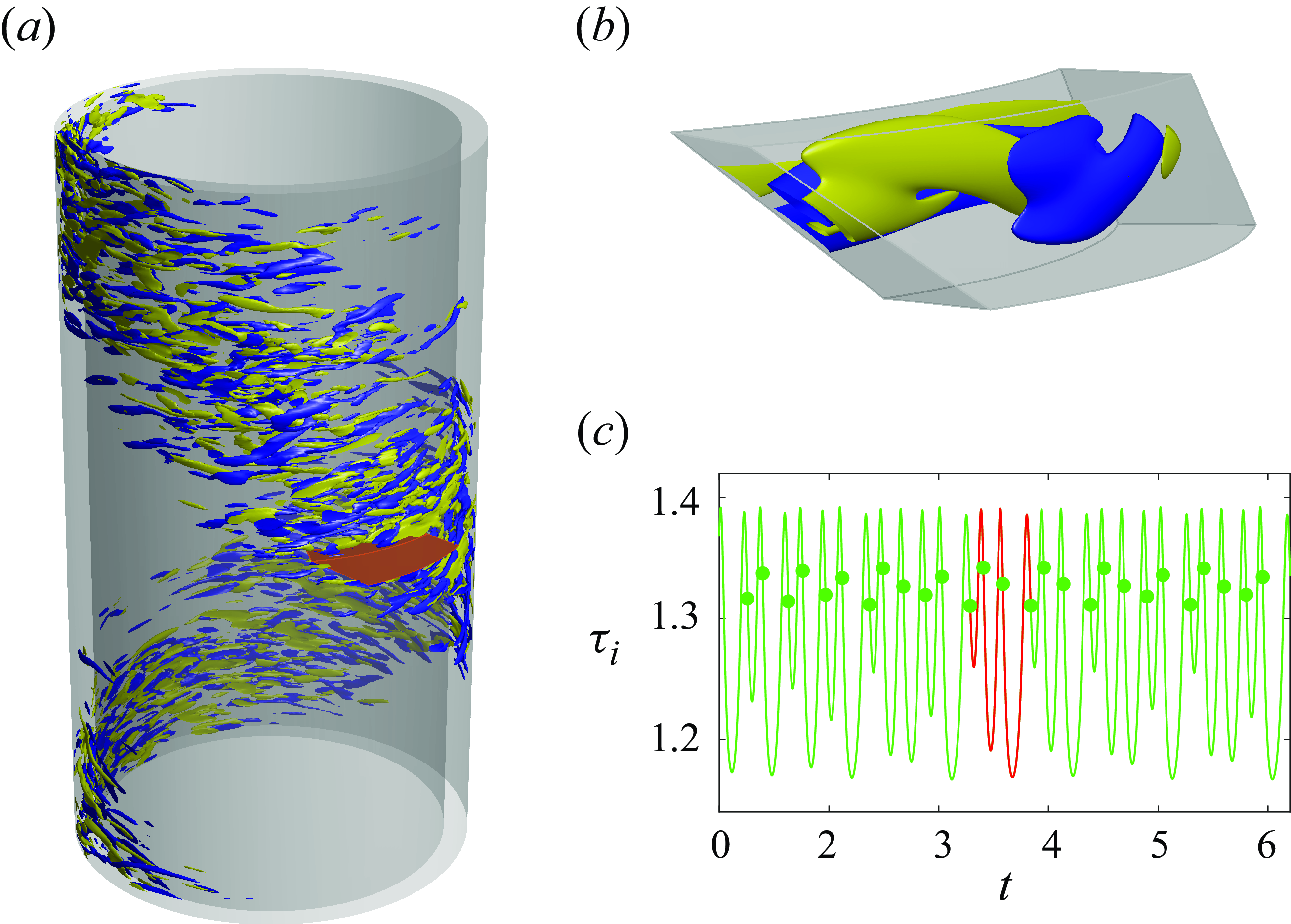
We target in our investigation the counter-rotating regime of Taylor–Couette flow, known for the subcritical onset of seemingly chaotic dynamics. The emergence of alternating turbulent and laminar helical bands (Coles Reference Coles1965) has puzzled physicists since its discovery (Feynman Reference Feynman1964). These peculiar flow structures (figure 1
a), which exhibit a clear-cut mean structure (Wang et al. Reference Wang, Mellibovsky, Ayats, Deguchi and Meseguer2023), act as harbingers of full-fledged turbulence (Andereck, Liu & Swinney Reference Andereck, Liu and Swinney1986). Constraining the turbulent motions within the stripes to small computational domains of parallelogram-annular shape (the small orange box in figure 1
a and the domain of figure 1
b), which can be regarded as a minimal flow unit (Jimenez & Moin Reference Jimenez and Moin1991; Hamilton, Kim & Waleffe Reference Hamilton, Kim and Waleffe1995) for the small-scale structures – about the smallest that can sustain turbulence at sufficiently large rotation rates – has been recently found to significantly tame the dynamics, thereby unveiling simple solutions (Wang et al. Reference Wang, Ayats, Deguchi, Mellibovsky and Meseguer2022). In this domain, and for the right set of dynamical parameters, the route to chaos begins with a Feigenbaum cascade (Wang et al. Reference Wang, Ayats, Deguchi, Mellibovsky and Meseguer2024) as shown in figure 2(a). We shall shortly see that, some distance past the accumulation point ( $R_\infty$
), an unstable period-3 orbit (P
$R_\infty$
), an unstable period-3 orbit (P $_3$
, red triangles) can be identified.
$_3$
, red triangles) can be identified.
Taylor–Couette problem. (a) The spiral turbulence regime visualised by isosurfaces of azimuthal vorticity. The small parallelogram-annular domain in orange is the minimal flow unit used throughout this paper, adopted from Wang et al. (Reference Wang, Ayats, Deguchi, Mellibovsky and Meseguer2022). (b) Snapshot of the P $_3$
solution in the minimal flow unit at a value of the inner cylinder Reynolds number
$_3$
solution in the minimal flow unit at a value of the inner cylinder Reynolds number $R_i=395.7816$
(see definition in the text). (c) The DNS time signal of inner torque
$R_i=395.7816$
(see definition in the text). (c) The DNS time signal of inner torque $\tau _i$
. Circles denote crossings of the Poincaré section
$\tau _i$
. Circles denote crossings of the Poincaré section $\Sigma$
. The red portion indicates a transient approach to
$\Sigma$
. The red portion indicates a transient approach to $\mathrm {P}_3$
.
$\mathrm {P}_3$
.
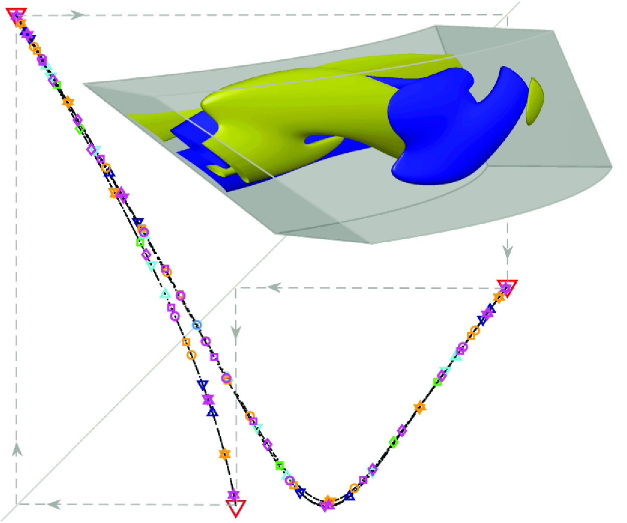
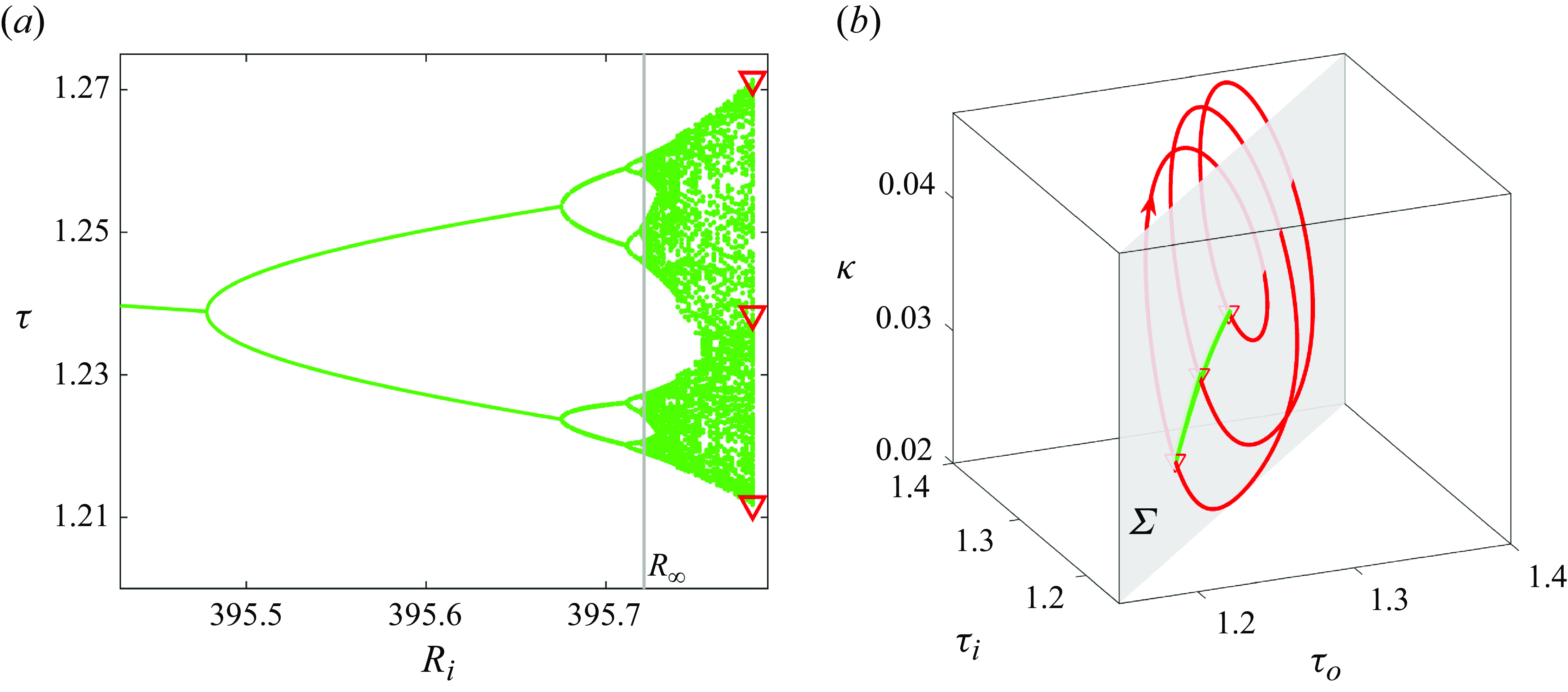
Attractor (from DNS data) and the period-3 orbit (converged with the Poincaré-Newton-Krylov method, PNK). (a) The bifurcation diagram generating the chaotic set. The green dots show torque $\tau$
(on the Poincaré section
$\tau$
(on the Poincaré section $\Sigma$
) as a function of the inner cylinder Reynolds number
$\Sigma$
) as a function of the inner cylinder Reynolds number $R_i$
for statistically steady states in DNS. The red triangles indicate the period-3 orbit (P
$R_i$
for statistically steady states in DNS. The red triangles indicate the period-3 orbit (P $_3$
) at
$_3$
) at $R_i=395.7816$
, at some distance beyond the cascade’s accumulation point
$R_i=395.7816$
, at some distance beyond the cascade’s accumulation point $R_\infty$
. (b) Phase map projection on
$R_\infty$
. (b) Phase map projection on $(\tau _i,\tau _o,\kappa )$
of the P
$(\tau _i,\tau _o,\kappa )$
of the P $_3$
orbit (red line) and a representation of the chaotic attractor on the Poincaré section
$_3$
orbit (red line) and a representation of the chaotic attractor on the Poincaré section $\Sigma$
(green dots) at
$\Sigma$
(green dots) at $R_i=395.7816$
.
$R_i=395.7816$
.
Our computational set-up deals with an incompressible fluid of kinematic viscosity $\nu$
confined between two coaxial cylinders of inner and outer radii
$\nu$
confined between two coaxial cylinders of inner and outer radii $r_i$
and
$r_i$
and $r_o$
, respectively. The inner and outer cylinders are independently rotating with respect to their common axis at angular speeds
$r_o$
, respectively. The inner and outer cylinders are independently rotating with respect to their common axis at angular speeds $\Omega _i$
and
$\Omega _i$
and $\Omega _o$
. The fluid motion is governed by the Navier–Stokes equations,
$\Omega _o$
. The fluid motion is governed by the Navier–Stokes equations,
 \begin{eqnarray} \partial _{t}\mathbf {v} + (\mathbf {v} \boldsymbol{\cdot} \nabla )\mathbf {v} = -\nabla (p-zf(t)) + \nabla ^{2}\mathbf {v}, \end{eqnarray}
expressed in non-dimensional form, using the radial gap $d=r_o-r_i$
and
$d=r_o-r_i$
and $d^2/\nu$
as units of length and time, respectively. This scaling leads to the inner,
$d^2/\nu$
as units of length and time, respectively. This scaling leads to the inner, $R_i= dr_i\Omega _i/\nu$
, and outer,
$R_i= dr_i\Omega _i/\nu$
, and outer, $R_o=dr_o\Omega _o/\nu$
, Reynolds numbers associated with the rotation of the inner and outer cylinders, respectively. The pressure gradient consists of two components: an axial forcing term (
$R_o=dr_o\Omega _o/\nu$
, Reynolds numbers associated with the rotation of the inner and outer cylinders, respectively. The pressure gradient consists of two components: an axial forcing term ( $f \hat{\textbf{z}}$
) that adjusts instantaneously to keep zero-axial net mass flux, and the rest (
$f \hat{\textbf{z}}$
) that adjusts instantaneously to keep zero-axial net mass flux, and the rest ( $\nabla p$
) that constrains the velocity (
$\nabla p$
) that constrains the velocity ( $\textbf {v}$
) to comply with the incompressibility condition
$\textbf {v}$
) to comply with the incompressibility condition $\nabla \boldsymbol{\cdot} \mathbf {v} = 0$
. For convenience, we employ cylindrical coordinates
$\nabla \boldsymbol{\cdot} \mathbf {v} = 0$
. For convenience, we employ cylindrical coordinates $(r,\theta ,z)$
. The boundary conditions at the inner and outer cylinder walls
$(r,\theta ,z)$
. The boundary conditions at the inner and outer cylinder walls $r=r_i$
and
$r=r_i$
and $r=r_o$
are
$r=r_o$
are $\mathbf {v}=R_i\,\hat {{\boldsymbol {\theta }}}$
and
$\mathbf {v}=R_i\,\hat {{\boldsymbol {\theta }}}$
and $\mathbf {v}=R_o\,\hat {{\boldsymbol {\theta }}}$
. Periodicity is enforced to the rest of the boundaries of the parallelogram domain (see figure 1
b, illustrated with a snapshot of P
$\mathbf {v}=R_o\,\hat {{\boldsymbol {\theta }}}$
. Periodicity is enforced to the rest of the boundaries of the parallelogram domain (see figure 1
b, illustrated with a snapshot of P $_3$
). In our particular set-up, the radius ratio is
$_3$
). In our particular set-up, the radius ratio is $\eta =r_i/r_o=0.883$
, and the outer cylinder Reynolds number is fixed at
$\eta =r_i/r_o=0.883$
, and the outer cylinder Reynolds number is fixed at $R_o=-1200$
. The transition scenario for these parameter values and increasing inner cylinder Reynolds number
$R_o=-1200$
. The transition scenario for these parameter values and increasing inner cylinder Reynolds number $R_i$
has been thoroughly studied (Meseguer et al. Reference Meseguer, Mellibovsky, Avila and Marques2009; Deguchi et al. Reference Deguchi, Meseguer and Mellibovsky2014; Wang et al. Reference Wang, Ayats, Deguchi, Mellibovsky and Meseguer2022). The DNS is performed using a fourth-order linearly implicit (IMEX) scheme, and UPOs are computed with the Poincaré–Newton–Krylov (PNK) method detailed in Wang et al. (Reference Wang, Ayats, Deguchi, Mellibovsky and Meseguer2022) and using the same numerical set-up in terms of domain shape, size and resolution.
$R_i$
has been thoroughly studied (Meseguer et al. Reference Meseguer, Mellibovsky, Avila and Marques2009; Deguchi et al. Reference Deguchi, Meseguer and Mellibovsky2014; Wang et al. Reference Wang, Ayats, Deguchi, Mellibovsky and Meseguer2022). The DNS is performed using a fourth-order linearly implicit (IMEX) scheme, and UPOs are computed with the Poincaré–Newton–Krylov (PNK) method detailed in Wang et al. (Reference Wang, Ayats, Deguchi, Mellibovsky and Meseguer2022) and using the same numerical set-up in terms of domain shape, size and resolution.
We characterise flow states by the inner $\tau _i$
and outer
$\tau _i$
and outer $\tau _o$
cylinder torques. We also use the spatially averaged kinetic energy
$\tau _o$
cylinder torques. We also use the spatially averaged kinetic energy $\kappa$
of velocity deviation from the laminar circular Couette flow whenever a third observable is necessary. All quantities are normalised by their laminar value, such that
$\kappa$
of velocity deviation from the laminar circular Couette flow whenever a third observable is necessary. All quantities are normalised by their laminar value, such that $\tau _i=\tau _o=1$
and
$\tau _i=\tau _o=1$
and $\kappa =0$
for circular Couette flow. We use the torques to define the Poincaré section as
$\kappa =0$
for circular Couette flow. We use the torques to define the Poincaré section as
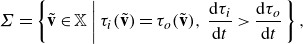 \begin{equation} \Sigma =\left \{\tilde {\textbf {v}}\in \mathbb {X}\left |\;\tau _i(\tilde {\textbf {v}})=\tau _o({\tilde {\textbf {v}}}),\;\dfrac {{\rm d}\tau _i}{{\rm d}t}\gt \dfrac {{\rm d}\tau _o}{{\rm d}t}\right. \right \}, \end{equation}
where $\tilde {\mathbf {v}}$
is the velocity field
$\tilde {\mathbf {v}}$
is the velocity field $\mathbf {v}$
, duly shifted with the method of slices (Willis, Cvitanovic & Avila Reference Willis, Cvitanovic and Avila2013; Wang et al. Reference Wang, Mellibovsky, Ayats, Deguchi and Meseguer2023) to remove the degeneracy induced by the spatial drift of the solutions, both in the axial and azimuthal directions, and
$\mathbf {v}$
, duly shifted with the method of slices (Willis, Cvitanovic & Avila Reference Willis, Cvitanovic and Avila2013; Wang et al. Reference Wang, Mellibovsky, Ayats, Deguchi and Meseguer2023) to remove the degeneracy induced by the spatial drift of the solutions, both in the axial and azimuthal directions, and $\mathbb {X}$
is the corresponding phase space. The bifurcation diagram shown in figure 2(a) records the torque, on
$\mathbb {X}$
is the corresponding phase space. The bifurcation diagram shown in figure 2(a) records the torque, on $\Sigma$
, of statistically steady states. Beyond the accumulation point of the cascade,
$\Sigma$
, of statistically steady states. Beyond the accumulation point of the cascade, $R_{\infty }$
, the seemingly chaotic attractor forms banded structures in the bifurcation diagram that progressively widen and successively merge in pairs.
$R_{\infty }$
, the seemingly chaotic attractor forms banded structures in the bifurcation diagram that progressively widen and successively merge in pairs.
Hereafter, we will focus on $R_i=395.7816$
. The energy and torque DNS signals occasionally produce nearly periodic timestamps at this value of the parameter (figure 1
c). States taken from selected pseudo-periodic lapses converge onto UPOs when fed to the PNK scheme. A phase map projection of one such UPO is shown in figure 2(b). The trajectory pierces three times the Poincaré section every period, hence our naming it P
$R_i=395.7816$
. The energy and torque DNS signals occasionally produce nearly periodic timestamps at this value of the parameter (figure 1
c). States taken from selected pseudo-periodic lapses converge onto UPOs when fed to the PNK scheme. A phase map projection of one such UPO is shown in figure 2(b). The trajectory pierces three times the Poincaré section every period, hence our naming it P $_3$
(see figure 1
b for a snapshot of P
$_3$
(see figure 1
b for a snapshot of P $_3$
on
$_3$
on $\Sigma$
).
$\Sigma$
).
3. P $_3$
implies chaos
$_3$
implies chaos

It is well-known in chaos theory that for 1-D (one-dimensional) maps generated by continuous functions $f\!: I\rightarrow I$
, where
$f\!: I\rightarrow I$
, where $I\subset \mathbb {R}$
is an interval, the advent of period-3 orbits holds a special significance. Specifically, as established by Li & Yorke (Reference Li and Yorke1975), it implies chaos in the sense that the map enhances a swift mixing of the points in the interval. Moreover, according to Sharkovskii’s theorem (Sharkovskii Reference Sharkovskii1964), the presence of a period-3 point entails also the existence of infinitely many periodic points.
$I\subset \mathbb {R}$
is an interval, the advent of period-3 orbits holds a special significance. Specifically, as established by Li & Yorke (Reference Li and Yorke1975), it implies chaos in the sense that the map enhances a swift mixing of the points in the interval. Moreover, according to Sharkovskii’s theorem (Sharkovskii Reference Sharkovskii1964), the presence of a period-3 point entails also the existence of infinitely many periodic points.
The presence of P $_3$
in our system therefore renders the application of the Li–Yorke and Sharkovskii theorems highly enticing. However, the theorems hinge upon an imperative condition: the map must be 1-D and continuous. These theorems might not hold true for higher dimensional systems, even if period-3 orbits were in existence. While instances of period-3 solutions abound in the fluid dynamics literature (Moore et al. Reference Moore, Toomre, Knobloch and Weiss1983; Knobloch et al. Reference Knobloch, Moore, Toomre and Weiss1986; Kreilos & Eckhardt Reference Kreilos and Eckhardt2012), no study has positively checked, to the best of our knowledge, the conditions for the validity of these theorems.
$_3$
in our system therefore renders the application of the Li–Yorke and Sharkovskii theorems highly enticing. However, the theorems hinge upon an imperative condition: the map must be 1-D and continuous. These theorems might not hold true for higher dimensional systems, even if period-3 orbits were in existence. While instances of period-3 solutions abound in the fluid dynamics literature (Moore et al. Reference Moore, Toomre, Knobloch and Weiss1983; Knobloch et al. Reference Knobloch, Moore, Toomre and Weiss1986; Kreilos & Eckhardt Reference Kreilos and Eckhardt2012), no study has positively checked, to the best of our knowledge, the conditions for the validity of these theorems.
A very long DNS (over 500 viscous time units) was conducted, with the solution $\tilde {\textbf {v}}(t_j)$
recorded at the chronologically ordered discrete times
$\tilde {\textbf {v}}(t_j)$
recorded at the chronologically ordered discrete times $t_j$
,
$t_j$
, $j=0,1,2,\dots$
, at which the phase map trajectory crosses the Poincaré section
$j=0,1,2,\dots$
, at which the phase map trajectory crosses the Poincaré section $\Sigma$
. The approximately 2500 data points we collected are shown as green dots in figure 2(b). All points are tightly clustered on a very narrow band, akin to a 1-D curve. This holds for any projection of
$\Sigma$
. The approximately 2500 data points we collected are shown as green dots in figure 2(b). All points are tightly clustered on a very narrow band, akin to a 1-D curve. This holds for any projection of $\mathbb {X}$
one might choose, which indicates a highly restricted dimensionality of the first return (Poincaré) map
$\mathbb {X}$
one might choose, which indicates a highly restricted dimensionality of the first return (Poincaré) map $\Phi: \Sigma \longrightarrow \Sigma$
. Strictly speaking, the dimension cannot be exactly one in the case of reversible maps but, as demonstrated by well-known examples such as the Hénon map or the Lorenz system, it can approach one. Indeed, since our system is at a relatively low Reynolds number, it is plausible that the dimension of the inertial manifold (Temam Reference Temam1989; Ding et al. Reference Ding, Chaté, Cvitanović, Siminos and Takeuchi2016; Haller et al. Reference Haller, Kaszás, Liu and Axås2023) might be particularly low. Figure 3(a) shows the return map in terms of the torque
$\Phi: \Sigma \longrightarrow \Sigma$
. Strictly speaking, the dimension cannot be exactly one in the case of reversible maps but, as demonstrated by well-known examples such as the Hénon map or the Lorenz system, it can approach one. Indeed, since our system is at a relatively low Reynolds number, it is plausible that the dimension of the inertial manifold (Temam Reference Temam1989; Ding et al. Reference Ding, Chaté, Cvitanović, Siminos and Takeuchi2016; Haller et al. Reference Haller, Kaszás, Liu and Axås2023) might be particularly low. Figure 3(a) shows the return map in terms of the torque $\tau (j)\equiv \tau _i(\tilde {\textbf {v}}(t_j))=\tau _o(\tilde {\textbf {v}}(t_j))$
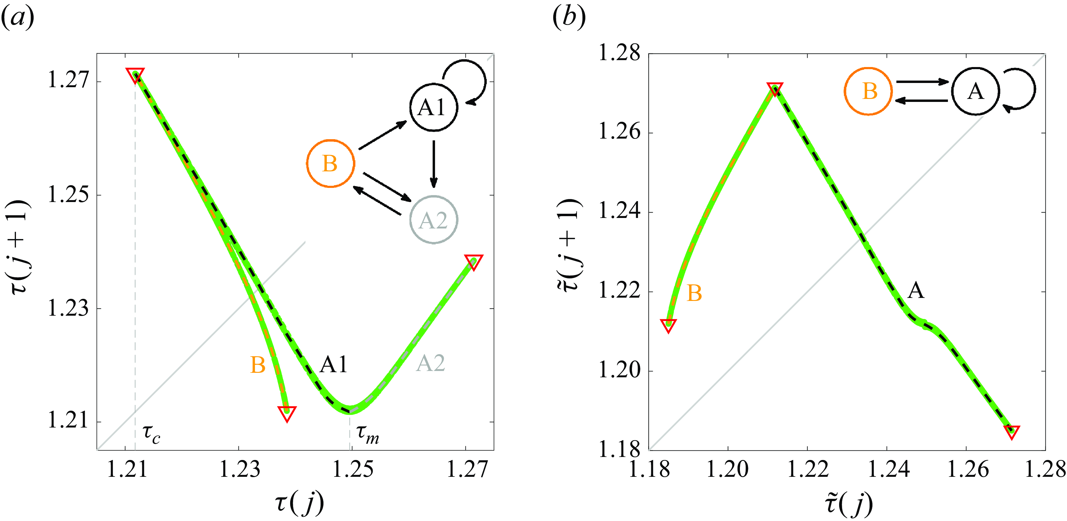
. The multivaluedness of the map hinders direct application of standard 1-D dynamical systems theory, but this can be readily addressed by simple identification of the selection rule among branches. The curve in figure 3(a) is naturally split at the cusp point
$\tau (j)\equiv \tau _i(\tilde {\textbf {v}}(t_j))=\tau _o(\tilde {\textbf {v}}(t_j))$
. The multivaluedness of the map hinders direct application of standard 1-D dynamical systems theory, but this can be readily addressed by simple identification of the selection rule among branches. The curve in figure 3(a) is naturally split at the cusp point $\tau =\tau _c$
into two main branches: A (grey scale) and B (orange). Branch A is then further split in two sub-branches, A1 (dark) and A2 (light), for convenience. The diagram in the inset summarises the selection rule among branches. A point on branch A1 might be mapped onto itself or sent to branch A2 and thence immediately to branch B. Then branch B instantly repels the trajectory, but whether A1 or A2 is to follow depends on the landing location along the branch.
$\tau =\tau _c$
into two main branches: A (grey scale) and B (orange). Branch A is then further split in two sub-branches, A1 (dark) and A2 (light), for convenience. The diagram in the inset summarises the selection rule among branches. A point on branch A1 might be mapped onto itself or sent to branch A2 and thence immediately to branch B. Then branch B instantly repels the trajectory, but whether A1 or A2 is to follow depends on the landing location along the branch.
A single-valued version of the map can then be constructed by applying the change of variable
 \begin{equation} \tilde {\tau }(j) = \left \{ \begin{array}{l@{\quad}l} 2\tau _c-\tau (j) & \text {if $\tau (j-1)\gt \tau _m$} \\ \tau (j) & \mathrm {otherwise} \end{array} \right.\!, \end{equation}
where $\tau _m \approx 1.250$
is the location of the local minimum of the multivalued function, whose immediate surroundings are mapped to the vicinity of
$\tau _m \approx 1.250$
is the location of the local minimum of the multivalued function, whose immediate surroundings are mapped to the vicinity of $\tau _c \approx 1.212$
. This change of variable corresponds effectively to the unfolding of the map, shown in figure 3(b), which now admits standard cob-webbing to monitor the dynamics. By interpolating the DNS data points and P
$\tau _c \approx 1.212$
. This change of variable corresponds effectively to the unfolding of the map, shown in figure 3(b), which now admits standard cob-webbing to monitor the dynamics. By interpolating the DNS data points and P $_3$
using splines, it is possible to construct a continuous function
$_3$
using splines, it is possible to construct a continuous function $S:I \rightarrow I$
, where
$S:I \rightarrow I$
, where $I\approx [1.185,1.271]$
. The spline dynamical system
$I\approx [1.185,1.271]$
. The spline dynamical system $\tilde {\tau }(j+1)=S(\tilde {\tau }(j))$
is chaotic in the Li–Yorke sense, because it contains the P
$\tilde {\tau }(j+1)=S(\tilde {\tau }(j))$
is chaotic in the Li–Yorke sense, because it contains the P $_3$
points, which in this case appear at the vertex and endpoints of the continuous function
$_3$
points, which in this case appear at the vertex and endpoints of the continuous function $S$
.
$S$
.
Return map analyses based on the Poincaré map on $\Sigma$
at
$\Sigma$
at $R_i=395.7816$
. (a) Return map of the chaotic attractor (green dots) and of P
$R_i=395.7816$
. (a) Return map of the chaotic attractor (green dots) and of P $_3$
(red triangles). The cusp (
$_3$
(red triangles). The cusp ( $\tau _c$
) and minimum (
$\tau _c$
) and minimum ( $\tau _m$
) points split the map in three distinct branches: B (orange), A1 (black) and A2 (grey). (b) The same return map, now unfolded following (3.1). The A1 and A2 branches are now labelled as A (black). The inset diagrams in (a) and (b) indicate branch selection rules.
$\tau _m$
) points split the map in three distinct branches: B (orange), A1 (black) and A2 (grey). (b) The same return map, now unfolded following (3.1). The A1 and A2 branches are now labelled as A (black). The inset diagrams in (a) and (b) indicate branch selection rules.
The PDF for the spline dynamical system (black), the normalised histogram for DNS data of the chaotic attractor (green), and the prediction from periodic points (grey).
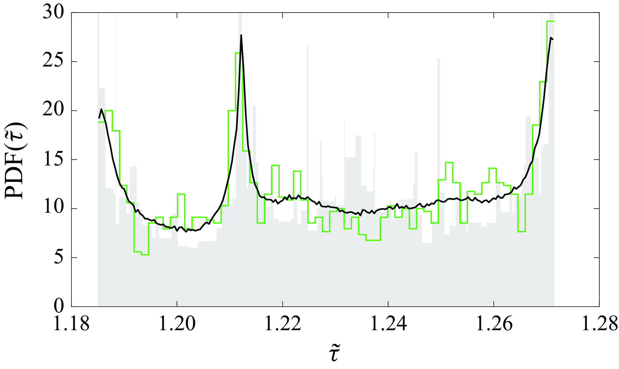
A natural question follows regarding the extent to which iteration of the spline map reproduces DNS results, an issue that needs assessing. To this end, we compare the probability density functions (PDFs) in figure 4. The PDF corresponding to the spline dynamical system (black curve), with its Lyapunov exponent of approximately $0.47$
, excellently matches the DNS results (green curve). The emergence of peaks in the PDF around the period-3 points is a common feature of the intermittency route to chaos (Pomeau & Manneville Reference Pomeau and Manneville1980; Eckmann Reference Eckmann1981).
$0.47$
, excellently matches the DNS results (green curve). The emergence of peaks in the PDF around the period-3 points is a common feature of the intermittency route to chaos (Pomeau & Manneville Reference Pomeau and Manneville1980; Eckmann Reference Eckmann1981).
4. Probability density function computed from unstable periodic solutions
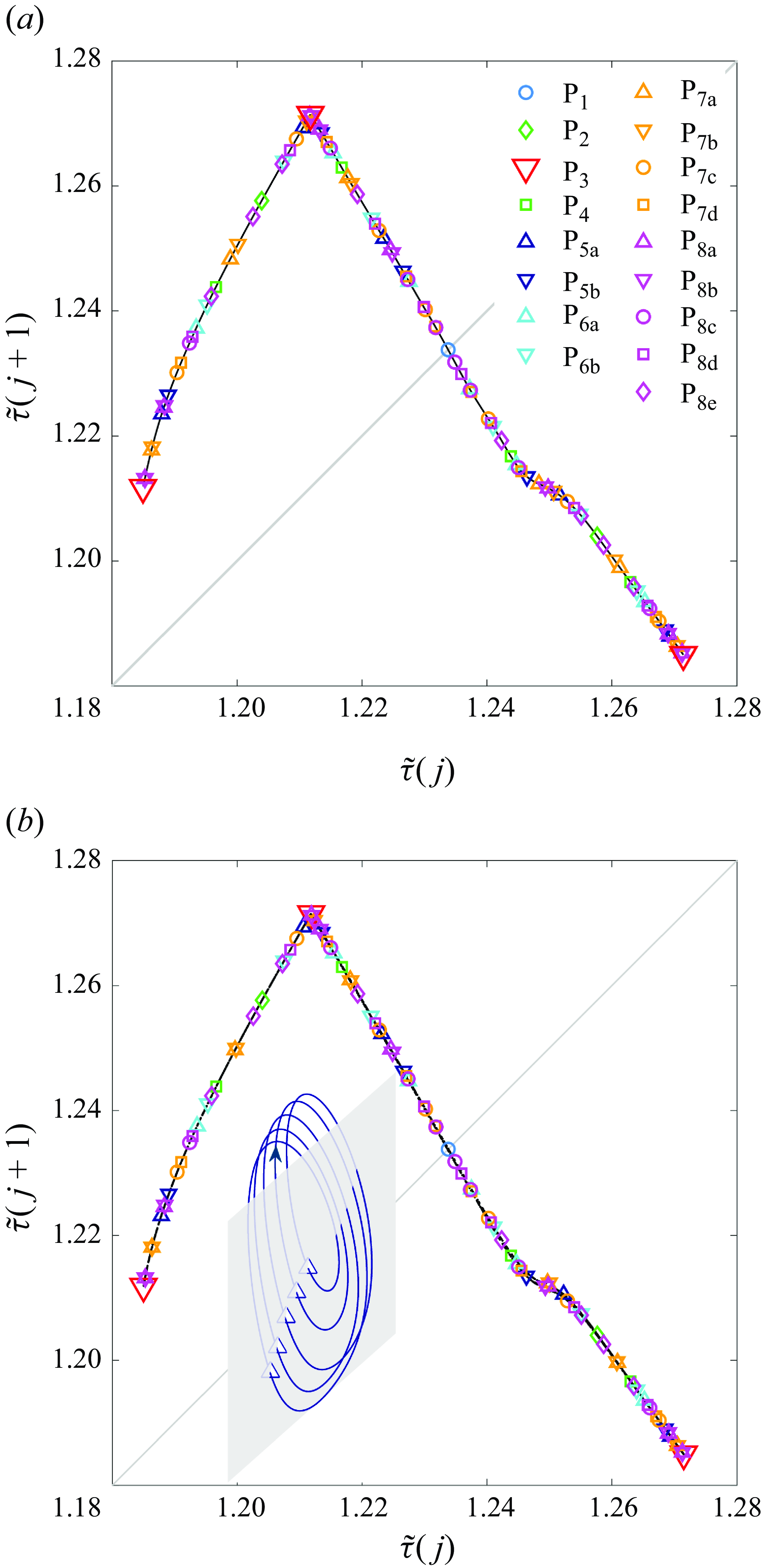
The inherent relation between the spline dynamical system and the Navier–Stokes dynamics becomes all the more evident through the comparison of periodic solutions. For the 1-D spline map, Sharkovskii’s theorem guarantees the existence of periodic points of period $n$
for every
$n$
for every $n \in \mathbb {N}$
. Figure 5(a) shows the complete set up to
$n \in \mathbb {N}$
. Figure 5(a) shows the complete set up to $n=8$
. We have been able to find the Navier–Stokes counterpart to each and every one of the spline periodic points employing PNK (see figure 5
b). The discrepancy in terms of torque between spline map and the Navier–Stokes solutions is consistently below
$n=8$
. We have been able to find the Navier–Stokes counterpart to each and every one of the spline periodic points employing PNK (see figure 5
b). The discrepancy in terms of torque between spline map and the Navier–Stokes solutions is consistently below $0.25\, \%$
.
$0.25\, \%$
.
Complete set of periodic points up to period $n=8$
for (a) the spline map approximation and (b) the Navier–Stokes system. The inset shows a phase map projection of P
$n=8$
for (a) the spline map approximation and (b) the Navier–Stokes system. The inset shows a phase map projection of P $_{5a}$
analogous to that of P
$_{5a}$
analogous to that of P $_3$
in figure 3(a).
$_3$
in figure 3(a).
The fluid flow scenario we have chosen is accurately described by a map of great mathematical simplicity, whose elegant attributes make it possible to infer the PDF of chaotic dynamics from the underlying periodic points in a clear and straightforward manner. First we note that the branch selection of the unfolded map, shown in the inset of figure 3(b), is extremely simple, with B and A representing the branches to the left and right of the maximum, respectively. The diagram is nothing but the topological Markov chain over the alphabet $\{A, B\}$
, whose topological entropy is known to be the natural logarithm of the golden ratio
$\{A, B\}$
, whose topological entropy is known to be the natural logarithm of the golden ratio $\phi =(1+\sqrt {5})/2$
(see Cvitanović et al. (Reference Cvitanović, Artuso, Mainieri, Tanner and Vattay2016) for the derivation). The spline map being an interval map of strictly positive entropy, one can conclude that it must be chaotic in the sense of Devaney (Li Reference Li1993; Devaney Reference Devaney2022). The periodic points are, therefore, densely distributed within the chaotic set, which supports the recurring assertion among fluid dynamicists that UPOs form the skeleton of turbulence (Kawahara et al. Reference Kawahara, Uhlmann and van Veen2012; Graham & Floryan Reference Graham and Floryan2021; Crowley et al. Reference Crowley, Pugue-Sanford, Toler, Krygier, Grigoriev and Schatz2022; Avila, Barkley & Hof Reference Avila, Barkley and Hof2023). The 100 periodic points we have computed cover the map effectively, thus suggesting that UPOs indeed encode the dynamics and, consequently, hold the key to predicting the statistical properties inherent to chaos.
$\phi =(1+\sqrt {5})/2$
(see Cvitanović et al. (Reference Cvitanović, Artuso, Mainieri, Tanner and Vattay2016) for the derivation). The spline map being an interval map of strictly positive entropy, one can conclude that it must be chaotic in the sense of Devaney (Li Reference Li1993; Devaney Reference Devaney2022). The periodic points are, therefore, densely distributed within the chaotic set, which supports the recurring assertion among fluid dynamicists that UPOs form the skeleton of turbulence (Kawahara et al. Reference Kawahara, Uhlmann and van Veen2012; Graham & Floryan Reference Graham and Floryan2021; Crowley et al. Reference Crowley, Pugue-Sanford, Toler, Krygier, Grigoriev and Schatz2022; Avila, Barkley & Hof Reference Avila, Barkley and Hof2023). The 100 periodic points we have computed cover the map effectively, thus suggesting that UPOs indeed encode the dynamics and, consequently, hold the key to predicting the statistical properties inherent to chaos.
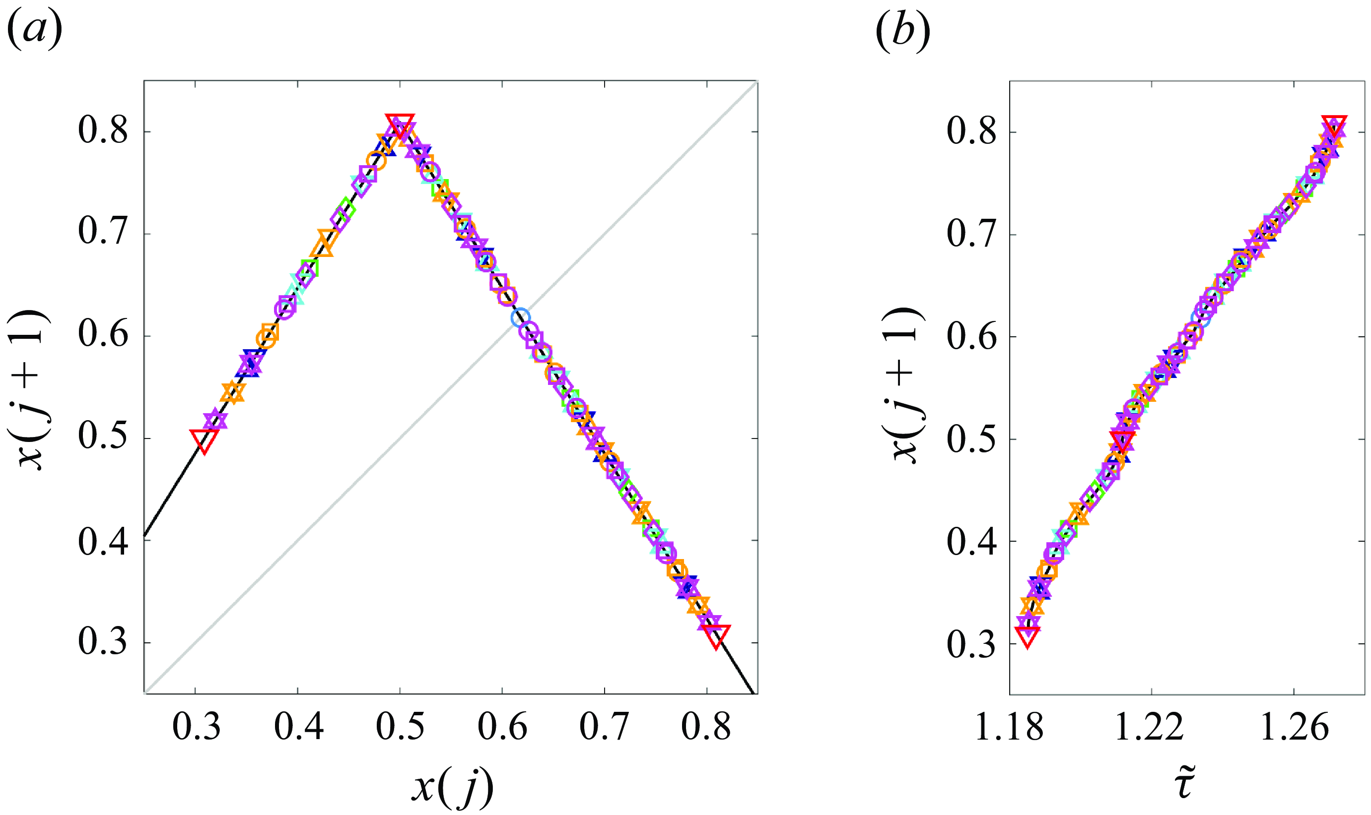
Topological conjugacy of the tent and spline maps. (a) The tent map $T(x)$
with all periodic points up to period
$T(x)$
with all periodic points up to period $n\leq 8$
. (b) Correspondence between tent map (ordinate) and spline map (abscissa) periodic points. The piecewise linear curve connecting the points provides an approximation of the conjugacy homeomorphism
$n\leq 8$
. (b) Correspondence between tent map (ordinate) and spline map (abscissa) periodic points. The piecewise linear curve connecting the points provides an approximation of the conjugacy homeomorphism $h(\tilde {\tau })$
. Symbols and colours, representing periodic orbits, follow the legend used in previous figures.
$h(\tilde {\tau })$
. Symbols and colours, representing periodic orbits, follow the legend used in previous figures.
The PDF of the spline map can be obtained from that of the tent map, $T(x) = \phi (1-|2x-1|)/2$
, with the scale parameter tuned to induce the appropriate topological Markov chain, i.e. having the same topological entropy
$T(x) = \phi (1-|2x-1|)/2$
, with the scale parameter tuned to induce the appropriate topological Markov chain, i.e. having the same topological entropy $\phi$
. Its PDF has a piecewise-constant closed analytical expression (Cvitanović et al. Reference Cvitanović, Artuso, Mainieri, Tanner and Vattay2016):
$\phi$
. Its PDF has a piecewise-constant closed analytical expression (Cvitanović et al. Reference Cvitanović, Artuso, Mainieri, Tanner and Vattay2016):
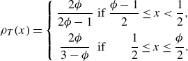 \begin{eqnarray} \rho _{T}(x)= \left \{ \begin{array}{ccr} \dfrac {2\phi }{2\phi -1} & \text {if} & \dfrac {\phi -1}{2}\leq x\lt \dfrac {1}{2},\\[1em] \dfrac {2\phi }{3-\phi } & \text {if} & \dfrac {1}{2} \leq x \leq \dfrac {\phi }{2}. \end{array} \right. \end{eqnarray}
Remarkably, the tent $T$
and spline
$T$
and spline $S$
maps share a common list of periodic solutions, appearing in the exact same order along the curve (figure 6
a). This implies the existence of a homeomorphism
$S$
maps share a common list of periodic solutions, appearing in the exact same order along the curve (figure 6
a). This implies the existence of a homeomorphism $h$
such that
$h$
such that $h(S(\tilde {\tau }))=T(h(\tilde {\tau }))$
, i.e. the two maps are topologically conjugate in the sense that they are dynamically equivalent (Yuan et al. Reference Yuan, Yorke, Carroll, Ott and Pecora2000). A discrete sampling of
$h(S(\tilde {\tau }))=T(h(\tilde {\tau }))$
, i.e. the two maps are topologically conjugate in the sense that they are dynamically equivalent (Yuan et al. Reference Yuan, Yorke, Carroll, Ott and Pecora2000). A discrete sampling of $h$
emerges naturally when plotting corresponding periodic points of the two maps on the
$h$
emerges naturally when plotting corresponding periodic points of the two maps on the $\tilde {\tau }$
–
$\tilde {\tau }$
– $x$
plane (figure 6
b). A straightforward calculation shows that the PDF of the spline and tent maps are related by
$x$
plane (figure 6
b). A straightforward calculation shows that the PDF of the spline and tent maps are related by $\rho _{S}(\tilde {\tau })=\rho _{T}(h(\tilde {\tau }))|h'(\tilde {\tau })|$
, where the prime denotes ordinary differentiation. The prediction, the grey shaded region shown in figure 4, is obtained from a piecewise linear approximation of
$\rho _{S}(\tilde {\tau })=\rho _{T}(h(\tilde {\tau }))|h'(\tilde {\tau })|$
, where the prime denotes ordinary differentiation. The prediction, the grey shaded region shown in figure 4, is obtained from a piecewise linear approximation of $h$
based on the available periodic points. The agreement with the spline and DNS data are fair despite the roughness of the estimation, as attested by the accurate reproduction of the three salient peaks.
$h$
based on the available periodic points. The agreement with the spline and DNS data are fair despite the roughness of the estimation, as attested by the accurate reproduction of the three salient peaks.
The prediction error in the PDF occurs primarily at high frequencies, thus having a small impact on the lower-order statistical moments. The expectation $E$
and variance
$E$
and variance $V$
of the torque computed from the PDFs are
$V$
of the torque computed from the PDFs are $(E,V)=(1.2294,6.9341 \times 10^{-4}), (1.2288,7.1341 \times 10^{-4})$
and
$(E,V)=(1.2294,6.9341 \times 10^{-4}), (1.2288,7.1341 \times 10^{-4})$
and $(1.2289, 6.9144 \times 10^{-4})$
, for the spline dynamical system, DNS and the UPOs prediction, respectively. Replacing the spline periodic points by the Navier–Stokes UPOs yields nearly the same results, as expected from the excellent agreement exhibited by figure 5. Furthermore, the 1-D assumption of the return map implies that the PDF for the full velocity field
$(1.2289, 6.9144 \times 10^{-4})$
, for the spline dynamical system, DNS and the UPOs prediction, respectively. Replacing the spline periodic points by the Navier–Stokes UPOs yields nearly the same results, as expected from the excellent agreement exhibited by figure 5. Furthermore, the 1-D assumption of the return map implies that the PDF for the full velocity field $\tilde {\mathbf {v}}$
can be determined in a similar manner. Therefore, all widely used turbulence statistics can, in principle, be computed using UPOs.
$\tilde {\mathbf {v}}$
can be determined in a similar manner. Therefore, all widely used turbulence statistics can, in principle, be computed using UPOs.
5. Conclusion
We have analysed, in the Taylor–Couette system, a subcritical parameter regime exhibiting dynamics that can be approximated by a simple discrete map. The map has exceptionally neat mathematical properties, which allow to rigorously establish its chaotic nature as well as the existence of infinitely many UPOs. Remarkably, the fluid system and the discrete map share a common catalogue of unstable periodic solutions with the tent map, a clear indication of topological conjugacy. A sufficient number of these solutions enables the construction of a conjugacy homeomorphism, which can be used to predict the PDF to be expected from DNS.
Our informed choice of scenario purposely aims at greatly simplifying the theoretical analysis. For more general cases, the topological properties of chaotic fluid systems could be approximated by simple Markov maps (Yalnız et al. Reference Yalnız, Hof and Budanur2021). As demonstrated in this paper, UPOs serve precisely as the link between such Markov maps and the Navier–Stokes system. Our theory differs from cycle expansion theory (Artuso et al. Reference Artuso, Aurell and Cvitanović1990; Cvitanović & Eckhardt Reference Cvitanović and Eckhardt1991; Christiansen et al. Reference Christiansen, Cvitanović and Putkaradze1997; Cvitanović et al. Reference Cvitanović, Artuso, Mainieri, Tanner and Vattay2016) and offers a more intuitive understanding of how the PDF can be constructed from UPOs. On the other hand, cycle expansion theory has the advantage of permitting the computation of statistically averaged quantities in a simpler manner by applying prescribed formulas.
A complete understanding of turbulence is still a long way off from both the applied and the mathematical stand points. Whether Hopf’s idea can be extended to high-Reynolds-number turbulence remains an open question. Furthermore, our results, depending on numerical approximations, do not guarantee that the Navier–Stokes solutions exhibit chaotic behaviour in the sense of Devaney. Nonetheless, we expect that our demonstration of how chaos theory applies to fluid flows under certain conditions will encourage future research on this important yet difficult problem.
Funding.
This research is supported by the Australian Research Council Discovery Project DP230102188 and the Ministerio de Ciencia, Innovación y Universidades (Agencia Estatal de Investigación, project nos PID 2020-114043 GB-I00 (MCIN/AEI/10.13039/501100011033) and PID 2023-150029NB-I00 (MCIN/AEI/10.13039/ 501100011033/FEDER, UE). B.W. and R.A.’s research has been funded by the European Union’s Horizon 2020 research and innovation programme (Marie Skłodowska-Curie grant agreement no. 101034413). R.A. has also been funded by the Austrian Science Fund (FWF) 10.55776/ESP1481224.
Declaration of interests.
The authors report no conflict of interest.


 Open access