


1. Introduction
Thermal convection plays a central role in many geophysical and astrophysical systems, such as mantle convection in terrestrial planets (e.g. Davies & Richards Reference Davies and Richards1992), core convection in planetary interiors (e.g. Wicht & Sanchez Reference Wicht and Sanchez2019), deep convection in the molecular layer of the gas giants (e.g. Aurnou et al. Reference Aurnou, Heimpel, Allen, King and Wicht2008) and stellar convection zones (e.g. Hanasoge, Gizon & Sreenivasan Reference Hanasoge, Gizon and Sreenivasan2016). The convective regions in most of these geophysical and astrophysical systems can be approximated as a spherical shell. For example, the Earth’s mantle convection takes place in a spherical shell geometry with a radius ratio of approximately $\eta = r_i / r_o \approx 0.55$
(Schubert, Turcotte & Olson Reference Schubert, Turcotte and Olson2001; Shahnas et al. Reference Shahnas, Lowman, Jarvis and Bunge2008), where
$\eta = r_i / r_o \approx 0.55$
(Schubert, Turcotte & Olson Reference Schubert, Turcotte and Olson2001; Shahnas et al. Reference Shahnas, Lowman, Jarvis and Bunge2008), where $r_i$
and
$r_i$
and $r_o$
are the radii of the inner and outer shell boundaries, respectively.
$r_o$
are the radii of the inner and outer shell boundaries, respectively.
Radially directed convection has also been proposed as a turbulence-driving mechanism in accretion disks (Teed & Latter Reference Teed and Latter2021). The cylindrical geometry of such disks motivates the study of convection between concentric cylinders under radially directed gravity as a simplified model. In laboratory experiments, a centrifugal force generated by strong mechanical rotation is often used to mimic radial gravity, commonly referred to as centrifugal convection (Jiang et al. Reference Jiang, Zhu, Wang, Huisman and Sun2020, Reference Jiang, Wang, Liu and Sun2022; Wang et al. Reference Wang, Jiang, Liu, Zhu and Sun2022; Zhong, Wang & Sun Reference Zhong, Wang and Sun2023; Wang et al. Reference Wang, Liu, Lai and Sun2024; Yao et al. Reference Yao, Emran, Teimurazov and Shishkina2025). These examples highlight the importance of understanding thermal convection in spherical and annular shell geometries.
Typically, spherical shell convection is studied in a spherical Rayleigh–Bénard convection (RBC) set-up, where a fluid is heated from inside and cooled from outside. A central question in the study of turbulent RBC is to understand how the dimensionless heat transport, characterised by the Nusselt number ( $ \textit{Nu}$
), scales with the dimensionless control parameters, which are the Rayleigh number (
$ \textit{Nu}$
), scales with the dimensionless control parameters, which are the Rayleigh number ( $ \textit{Ra}$
), the Prandtl number (
$ \textit{Ra}$
), the Prandtl number ( $ \textit{Pr}$
) and the parameters characterising the geometrical configuration. In turbulent RBC,
$ \textit{Pr}$
) and the parameters characterising the geometrical configuration. In turbulent RBC, $ \textit{Nu}$
is directly related to the temperature gradient across the thermal boundary layers (BLs) (e.g. Ahlers, Grossmann & Lohse Reference Ahlers, Grossmann and Lohse2009; Lohse & Xia Reference Lohse and Xia2010; Chillà & Schumacher Reference Chillà and Schumacher2012; Xia et al. Reference Xia, Huang, Xie and Zhang2023; Lohse & Shishkina Reference Lohse and Shishkina2024). The turbulent bulk flow induces a strong thermal mixing, so that most of the temperature drop occurs within the thermal BLs. As a result, determining the temperature drops and BL thicknesses is essential for predicting
$ \textit{Nu}$
is directly related to the temperature gradient across the thermal boundary layers (BLs) (e.g. Ahlers, Grossmann & Lohse Reference Ahlers, Grossmann and Lohse2009; Lohse & Xia Reference Lohse and Xia2010; Chillà & Schumacher Reference Chillà and Schumacher2012; Xia et al. Reference Xia, Huang, Xie and Zhang2023; Lohse & Shishkina Reference Lohse and Shishkina2024). The turbulent bulk flow induces a strong thermal mixing, so that most of the temperature drop occurs within the thermal BLs. As a result, determining the temperature drops and BL thicknesses is essential for predicting $ \textit{Nu}$
. In the framework of the Boussinesq approximation and with a planar geometry, the thermal BLs are symmetric near the top and bottom plates (Ahlers et al. Reference Ahlers, Grossmann and Lohse2009). Then, assuming that the entire temperature drop occurs within the BLs because of the strong thermal mixing in the bulk, each BL accounts for half of the total temperature difference between the hot and cold plates.
$ \textit{Nu}$
. In the framework of the Boussinesq approximation and with a planar geometry, the thermal BLs are symmetric near the top and bottom plates (Ahlers et al. Reference Ahlers, Grossmann and Lohse2009). Then, assuming that the entire temperature drop occurs within the BLs because of the strong thermal mixing in the bulk, each BL accounts for half of the total temperature difference between the hot and cold plates.
However, in curved geometries such as spherical and annular shells, curvature and non-uniform radial gravity lead to asymmetric thermal BLs. For instance, Gastine, Wicht & Aurnou (Reference Gastine, Wicht and Aurnou2015) and Fu et al. (Reference Fu, Bader, Song and Zhu2024) demonstrated through three-dimensional (3-D) simulations that, in spherical shells, the temperature drop across the inner BL is consistently greater than that across the outer one. This asymmetry is strongly dependent on the radius ratio $\eta$
and the radial gravity profile
$\eta$
and the radial gravity profile $g(r)$
, but remains largely unaffected by variations in
$g(r)$
, but remains largely unaffected by variations in $ \textit{Ra}$
. Similarly, Bhadra, Shishkina & Zhu (Reference Bhadra, Shishkina and Zhu2024) and Zhong, Li & Sun (Reference Zhong, Li and Sun2024) also observed such asymmetry in two-dimensional (2-D) annular RBC and sheared centrifugal convection, respectively. The thermal BL asymmetry is also observed in rotating spherical RBC, depending on
$ \textit{Ra}$
. Similarly, Bhadra, Shishkina & Zhu (Reference Bhadra, Shishkina and Zhu2024) and Zhong, Li & Sun (Reference Zhong, Li and Sun2024) also observed such asymmetry in two-dimensional (2-D) annular RBC and sheared centrifugal convection, respectively. The thermal BL asymmetry is also observed in rotating spherical RBC, depending on $\eta , Ra$
and the gravity profile (e.g. Gastine, Wicht & Aubert Reference Gastine, Wicht and Aubert2016; Long et al. Reference Long, Mound, Davies and Tobias2020; Wang et al. Reference Wang, Santelli, Lohse, Verzicco and Stevens2021; Hartmann et al. Reference Hartmann, Stevens, Lohse and Verzicco2024). Therefore, it is crucial to develop a physically grounded approach to quantify the thermal BL asymmetry in geometrically asymmetric RBC systems.
$\eta , Ra$
and the gravity profile (e.g. Gastine, Wicht & Aubert Reference Gastine, Wicht and Aubert2016; Long et al. Reference Long, Mound, Davies and Tobias2020; Wang et al. Reference Wang, Santelli, Lohse, Verzicco and Stevens2021; Hartmann et al. Reference Hartmann, Stevens, Lohse and Verzicco2024). Therefore, it is crucial to develop a physically grounded approach to quantify the thermal BL asymmetry in geometrically asymmetric RBC systems.
Previous efforts to quantify BL asymmetry have largely relied on intuitive or empirical assumptions. For example, in their study on non-Oberbeck–Boussinesq (NOB) convection, Wu & Libchaber (Reference Wu and Libchaber1991) assumed equal thermal fluctuation scales at the edges of the inner and outer thermal BLs, a finding later confirmed by Zhang, Childress & Libchaber (Reference Zhang, Childress and Libchaber1997). Wu & Libchaber (Reference Wu and Libchaber1991) derived an expression for BL asymmetry, which is represented by the bulk temperature and the BL thickness ratio, based on this assumption. In their experiments, the NOB effect comes from the temperature dependence of the thermal expansion coefficient, kinematic viscosity and thermal diffusivity. Similarly, Jarvis (Reference Jarvis1993) and Vangelov & Jarvis (Reference Vangelov and Jarvis1994) estimated the BL asymmetry in spherical and annular shells by assuming that the thermal BL Rayleigh numbers at the two boundaries are equal, i.e. $ \textit{Ra}_{i} = Ra_{o}$
with
$ \textit{Ra}_{i} = Ra_{o}$
with $ \textit{Ra}_{i,o} = \alpha \, g_{i,o}\, \Delta \theta _{i,o}\, (\lambda _{\vartheta }^{\,i,o})^{3}/(\nu \kappa )$
, where
$ \textit{Ra}_{i,o} = \alpha \, g_{i,o}\, \Delta \theta _{i,o}\, (\lambda _{\vartheta }^{\,i,o})^{3}/(\nu \kappa )$
, where $\alpha$
is the thermal expansion coefficient,
$\alpha$
is the thermal expansion coefficient, $\nu$
the kinematic viscosity and
$\nu$
the kinematic viscosity and $\kappa$
the thermal diffusivity. Here, the subscripts
$\kappa$
the thermal diffusivity. Here, the subscripts $i$
and
$i$
and $o$
denote quantities evaluated at the inner and outer boundaries (e.g.
$o$
denote quantities evaluated at the inner and outer boundaries (e.g. $g_{i,o}$
and
$g_{i,o}$
and $\Delta \theta _{i,o}$
), while the superscripts
$\Delta \theta _{i,o}$
), while the superscripts $i$
and
$i$
and $o$
refer to the corresponding inner and outer thermal BL thicknesses
$o$
refer to the corresponding inner and outer thermal BL thicknesses $\lambda _{\vartheta }^{i}$
and
$\lambda _{\vartheta }^{i}$
and $\lambda _{\vartheta }^{o}$
. This assumption is motivated by the argument that neither BL is more unstable than the other.
$\lambda _{\vartheta }^{o}$
. This assumption is motivated by the argument that neither BL is more unstable than the other.
Gastine et al. (Reference Gastine, Wicht and Aurnou2015) tested these assumptions in spherical RBC at $ \textit{Pr}=1$
with various
$ \textit{Pr}=1$
with various $\eta$
and
$\eta$
and $g(r)$
and found them invalid under several gravity profiles. As an alternative, they proposed that the plume density is identical at both boundaries and derived a BL asymmetry expression from this assumption. However, its physical justification remains uncertain, and its generalisation to annular geometries is unclear. More recently, Bhadra et al. (Reference Bhadra, Shishkina and Zhu2024) assumed equal velocity scales for convective rolls at the inner and outer boundaries for 2-D annular RBC, leading to a BL asymmetry expression identical to that of Jarvis (Reference Jarvis1993). This result agrees with their simulations for
$g(r)$
and found them invalid under several gravity profiles. As an alternative, they proposed that the plume density is identical at both boundaries and derived a BL asymmetry expression from this assumption. However, its physical justification remains uncertain, and its generalisation to annular geometries is unclear. More recently, Bhadra et al. (Reference Bhadra, Shishkina and Zhu2024) assumed equal velocity scales for convective rolls at the inner and outer boundaries for 2-D annular RBC, leading to a BL asymmetry expression identical to that of Jarvis (Reference Jarvis1993). This result agrees with their simulations for $ \textit{Ra} \lesssim 10^{8}$
under a gravity profile of
$ \textit{Ra} \lesssim 10^{8}$
under a gravity profile of $g(r) \sim 1/r$
, where the Rayleigh number is defined as
$g(r) \sim 1/r$
, where the Rayleigh number is defined as $ \textit{Ra}=\alpha g \Delta T d^{3}/(\nu \kappa )$
, with
$ \textit{Ra}=\alpha g \Delta T d^{3}/(\nu \kappa )$
, with $d$
being the annular gap width. In addition, Fu, Bader & Zhu (Reference Fu, Bader and Zhu2025) assessed the validity of the heuristic assumptions discussed above in spherical shell convection with a centrally condensed gravity profile
$d$
being the annular gap width. In addition, Fu, Bader & Zhu (Reference Fu, Bader and Zhu2025) assessed the validity of the heuristic assumptions discussed above in spherical shell convection with a centrally condensed gravity profile $g\sim 1/r^2$
across a range of
$g\sim 1/r^2$
across a range of $0.1 \leq Pr \leq 50$
, and found that different assumptions become applicable in different
$0.1 \leq Pr \leq 50$
, and found that different assumptions become applicable in different $ \textit{Pr}$
regimes. In summary, all previous models for quantifying BL asymmetry rely on heuristic or empirical assumptions lacking rigorous physical justification. A comprehensive theory with a solid physical foundation that applies across various geometrical settings remains to be established.
$ \textit{Pr}$
regimes. In summary, all previous models for quantifying BL asymmetry rely on heuristic or empirical assumptions lacking rigorous physical justification. A comprehensive theory with a solid physical foundation that applies across various geometrical settings remains to be established.
Given that the asymmetry arises within the thermal BLs, an alternative approach is to analyse the asymmetry directly through BL theories. This method has been successfully applied in planar NOB RBC (e.g. Ahlers et al. Reference Ahlers, Brown, Araujo, Funfschilling, Grossmann and Lohse2006, Reference Ahlers, Araujo, Funfschilling, Grossmann and Lohse2007, Reference Ahlers, Calzavarini, Araujo, Funfschilling, Grossmann, Lohse and Sugiyama2008). In these works, the authors incorporated temperature-dependent fluid properties into the extended Prandtl–Blasius theory and solved the BL equations to determine the temperature drops at both boundaries. Motivated by their success, we extend this approach to geometries where BL asymmetry originates from curvature and gravity variations rather than fluid property gradients. We solve the BL equations rather than the full governing equations to quantify the BL asymmetry. This method avoids heuristic assumptions and allows a direct, physically motivated calculation of BL asymmetry, which is represented by the bulk temperature and the BL thickness ratio.
In this study, we employ three BL models, each of them being applicable in different regimes and under different conditions: the Prandtl–Blasius BL model (Prandtl Reference Prandtl1905; Blasius Reference Blasius1907; Pohlhausen Reference Pohlhausen1921), the steady free-convective BL model (Stewartson Reference Stewartson1958) and a BL theory which takes turbulent fluctuations into consideration (Ching et al. Reference Ching, Leung, Zwirner and Shishkina2019). These models are extended and adapted to the spherical and annular RBC configurations. The Oberbeck–Boussinesq approximation is employed in this study. It is widely used in modelling liquid-metal convection in planetary cores, where the flow is treated as incompressible and material properties are approximated as constants. We solve the BL equations for each case to predict the temperature drop across the BLs and compare the resulting asymmetries across different models and with data from direct numerical simulations (DNSs). Furthermore, we derive analytical expressions for the bulk temperature and the thermal BL thickness ratio from the BL models for both geometries. We obtain an approximate similarity streamfunction from its near-wall asymptotic behaviour within the BL. This enables analytical integration of the similarity thermal equations for both the inner and outer BLs. The bulk temperature and the BL thickness ratio are then obtained by closing the two BL solutions through a heat-flux matching condition. The resulting predictions show very good agreement with DNS data across all Prandtl-number regimes considered in this work.
The objectives of this study are threefold: (i) to use extended BL models to compute thermal BL asymmetry in spherical and annular RBC, and compare the predictions across models and with DNS data; (ii) to use DNS diagnostics to test the key assumptions of the BL models and to elucidate the origin of their differences; and (iii) to derive analytical solutions for BL asymmetry based on BL models. For the spherical shell configuration, we utilise simulation datasets from Gastine et al. (Reference Gastine, Wicht and Aurnou2015), Fu et al. (Reference Fu, Bader, Song and Zhu2024) and Fu et al. (Reference Fu, Bader and Zhu2025), and perform some additional high-Prandtl-number simulations (see table 4), which span a broad range of radius ratios, Rayleigh numbers, gravity profiles and Prandtl numbers. For the annular geometry, we perform our own 3-D simulations. For more details of the simulations, we refer the reader to § 2.2 and Appendix B.
The rest of the paper is organised as follows. Section 2 introduces the governing equations, numerical methods and observed BL asymmetries. Section 3 presents the extended BL models, including the governing similarity equations, boundary conditions and the matching conditions. Section 4 compares the predictions from BL models with DNS data. Section 5 provides analytical solutions derived for the BL asymmetry. Finally, § 6 summarises our main findings and outlines potential directions for future research.
Schematics of (a) spherical shell geometry and (b) annular shell geometry.

2. The asymmetry within the thermal BL of the spherical and annular RBC
2.1. Model description
We investigate RBC under the Oberbeck–Boussinesq approximation. The governing dimensional equations are given by
 \begin{align} \boldsymbol{\boldsymbol{\nabla }} \boldsymbol{\cdot } \boldsymbol{u} = 0, \\[-28pt] \nonumber \end{align}
 \begin{align} \frac {\partial \boldsymbol{u}}{\partial t} + \boldsymbol{u} \boldsymbol{\cdot } \boldsymbol{\boldsymbol{\nabla }} \boldsymbol{u} = -\frac {1}{\rho _{0}}\boldsymbol{\boldsymbol{\nabla }} p + \alpha g (T - T_{\textit{ref}})\boldsymbol{e_r} + \nu {{\nabla} }^2 \boldsymbol{u}, \\[-28pt] \nonumber \end{align}
 \begin{align} \frac {\partial T}{\partial t} + \boldsymbol{u} \boldsymbol{\cdot } \boldsymbol{\boldsymbol{\nabla }} T = \kappa {{\nabla} }^2 T. \\[-12pt] \nonumber \end{align}
Here, $\boldsymbol{u}$
represents the velocity field,
$\boldsymbol{u}$
represents the velocity field, $p$
denotes the pressure perturbation relative to the hydrostatic equilibrium state,
$p$
denotes the pressure perturbation relative to the hydrostatic equilibrium state, $T$
is the temperature and
$T$
is the temperature and $T_{\textit{ref}}$
is the reference temperature. Fluid properties, including the reference density
$T_{\textit{ref}}$
is the reference temperature. Fluid properties, including the reference density $\rho _{0}$
, thermal expansion coefficient
$\rho _{0}$
, thermal expansion coefficient $\alpha$
, kinematic viscosity
$\alpha$
, kinematic viscosity $\nu$
and thermal diffusivity
$\nu$
and thermal diffusivity $\kappa$
, are assumed constant. Gravity points radially inward and is a function of the radial location.
$\kappa$
, are assumed constant. Gravity points radially inward and is a function of the radial location.
We focus on two geometrical configurations: spherical shells and annular shells, as illustrated in figure 1. In the spherical shell geometry, convection occurs between an inner boundary at radius $r_i$
and an outer boundary at radius
$r_i$
and an outer boundary at radius $r_o$
, with gravity directed radially inward toward the centre of the sphere. At both boundaries, we enforce no-slip mechanical boundary conditions, and we assume them to be isothermal with fixed temperatures
$r_o$
, with gravity directed radially inward toward the centre of the sphere. At both boundaries, we enforce no-slip mechanical boundary conditions, and we assume them to be isothermal with fixed temperatures $T_{i}$
(hot) at the inner boundary and
$T_{i}$
(hot) at the inner boundary and $T_{o}$
(cold) at the outer boundary. Here, the no-slip mechanical boundary condition is adopted to mimic the planetary core convection, and the isothermal boundary condition is chosen for simplicity.
$T_{o}$
(cold) at the outer boundary. Here, the no-slip mechanical boundary condition is adopted to mimic the planetary core convection, and the isothermal boundary condition is chosen for simplicity.
In the annular shell geometry, convection takes place between two concentric cylindrical boundaries located at radii $r_i$
and
$r_i$
and $r_o$
, respectively. Gravity points inward toward the central
$r_o$
, respectively. Gravity points inward toward the central $z$
-axis. Similar to the spherical geometry, the radial boundaries are no-slip and isothermal, with fixed temperatures
$z$
-axis. Similar to the spherical geometry, the radial boundaries are no-slip and isothermal, with fixed temperatures $T_i$
at the inner boundary and
$T_i$
at the inner boundary and $T_o$
at the outer boundary. Periodic boundary conditions are applied in the axial (
$T_o$
at the outer boundary. Periodic boundary conditions are applied in the axial ( $z$
) direction.
$z$
) direction.
In our simulations, and throughout the analysis in this paper, we employ dimensionless variables. The variables are non-dimensionalised using the temperature scale $\Delta T = T_{i}-T_{o}$
, the length scale
$\Delta T = T_{i}-T_{o}$
, the length scale $d=r_{o}-r_{i}$
, the viscous time scale
$d=r_{o}-r_{i}$
, the viscous time scale $d^{2}/\nu$
, the velocity scale
$d^{2}/\nu$
, the velocity scale $\nu /d$
and the pressure scale
$\nu /d$
and the pressure scale $\rho \nu ^{2}/d^{2}$
. The dimensionless governing equations are shown in Appendix A. Dimensionless control parameters governing the dynamics can be defined from (A1)–(A3) as
$\rho \nu ^{2}/d^{2}$
. The dimensionless governing equations are shown in Appendix A. Dimensionless control parameters governing the dynamics can be defined from (A1)–(A3) as
 \begin{align} Ra = \frac {\alpha g_o \Delta T d^3}{\nu \kappa }, \quad Pr = \frac {\nu }{\kappa }, \end{align}
where $\Delta T = T_i - T_o$
is the imposed temperature difference between the boundaries. The geometrical parameters are
$\Delta T = T_i - T_o$
is the imposed temperature difference between the boundaries. The geometrical parameters are
 \begin{align} \eta = \frac {r_i}{r_o}, \quad \varGamma = \frac {L}{d}, \end{align}
where $L$
is the domain height and
$L$
is the domain height and $d = r_o - r_i$
is the radial gap width. The radius ratio
$d = r_o - r_i$
is the radial gap width. The radius ratio $\eta$
is employed for both spherical and annular geometries, while the aspect ratio
$\eta$
is employed for both spherical and annular geometries, while the aspect ratio $\varGamma$
is specifically used for annular geometry.
$\varGamma$
is specifically used for annular geometry.
We adopt the following notations throughout the paper for various averaging procedures. The overbar ( $\overline { {\cdots} }$
) denotes the time average of a variable
$\overline { {\cdots} }$
) denotes the time average of a variable $f$
, while
$f$
, while $\langle \boldsymbol{\cdot }\rangle s$
and
$\langle \boldsymbol{\cdot }\rangle s$
and $\langle \boldsymbol{\cdot }\rangle$
represent horizontal and volume averages, respectively. These averages are defined explicitly as
$\langle \boldsymbol{\cdot }\rangle$
represent horizontal and volume averages, respectively. These averages are defined explicitly as
 \begin{align} \overline {f} &= \frac {1}{\tau } \int _{t_0}^{t_0+\tau } f \mathrm{d} t, \\[-12pt] \nonumber \end{align}
 \begin{align} \left \langle f \right \rangle _{s}^{\textit{sp}} &= \frac {1}{4 \pi } \int _{0}^{\pi } \int _{0}^{2 \pi } f \sin {\theta } \mathrm{d}\theta \mathrm{d}\phi , \\[-12pt] \nonumber \end{align}
 \begin{align} \left \langle f \right \rangle _{s}^{\textit{an}} &= \frac {1}{2 \pi L} \int _{0}^{L} \int _{0}^{2 \pi } f \mathrm{d}\phi \mathrm{d}z, \\[-12pt] \nonumber \end{align}
 \begin{align} \left \langle f \right \rangle ^{\textit{sp}} &= \frac {1}{V_{\textit{sp}}} \int _{r_{i}}^{r_{o}} \int _{0}^{\pi } \int _{0}^{2 \pi } f\sin {\theta }\, r^{2} \mathrm{d}r \mathrm{d}\theta \mathrm{d}\phi , \\[-12pt] \nonumber \end{align}
 \begin{align} \left \langle f \right \rangle ^{\textit{an}} &= \frac {1}{V_{\textit{an}}} \int _{r_{i}}^{r_{o}} \int _{0}^{L} \int _{0}^{2 \pi } f\,r\, \mathrm{d}\phi \mathrm{d}z \mathrm{d}r. \\[10pt] \nonumber \end{align}
Here, superscripts ‘sp’ and ‘an’ indicate spherical and annular geometries, respectively. In these definitions, $\theta$
and
$\theta$
and $\phi$
represent colatitude and longitude for spherical shells, whereas
$\phi$
represent colatitude and longitude for spherical shells, whereas $\phi$
and
$\phi$
and $z$
denote azimuthal and axial directions for annular shells. The volumes of spherical and annular shells are
$z$
denote azimuthal and axial directions for annular shells. The volumes of spherical and annular shells are $V_{\textit{sp}}=4\pi (r_{o}^3-r_{i}^3)/3$
and
$V_{\textit{sp}}=4\pi (r_{o}^3-r_{i}^3)/3$
and $V_{\textit{an}}=\pi (r_{o}^2-r_{i}^2)L$
, respectively.
$V_{\textit{an}}=\pi (r_{o}^2-r_{i}^2)L$
, respectively.
There are two key response parameters in RBC: the Nusselt number ( $ \textit{Nu}$
), which represents the dimensionless heat flux, and the Reynolds number (
$ \textit{Nu}$
), which represents the dimensionless heat flux, and the Reynolds number ( $Re$
), which is a dimensionless measure of flow velocity. Under the Oberbeck–Boussinesq approximation, the Nusselt number with isothermal boundaries and the Reynolds number are defined as
$Re$
), which is a dimensionless measure of flow velocity. Under the Oberbeck–Boussinesq approximation, the Nusselt number with isothermal boundaries and the Reynolds number are defined as
 \begin{align} Nu = \frac {\overline {\left \langle u_{r}T \right \rangle _s} - \kappa \frac {{\rm d}\overline {\left \langle T \right \rangle _{s}}}{{\rm d}r}}{-\kappa \frac {{\rm d}T_c}{{\rm d}r}}, \quad Re = \overline {\sqrt {\left \langle \left | \boldsymbol{u} \right |^{2} \right \rangle }} \frac {d}{\nu }, \end{align}
respectively. Here, the conductive temperature profiles for spherical and annular shell geometries are given by
 \begin{align} \frac {\mathrm{d} T_{c}^{\textit{sp}}(r)}{\mathrm{d} r} = - \mathrm{\Delta } T \frac {\eta }{(1-\eta )^2} \frac {1}{r^{2}}, \quad \frac {\mathrm{d} T_{c}^{\textit{an}}(r)}{\mathrm{d} r} = \frac {\Delta T}{\ln {\eta }}\frac {1}{r}. \end{align}
By adopting the notations (2.6)–(2.8), the time- and horizontally averaged radial profiles of the temperature and the horizontal velocity are given, respectively, by
 \begin{align} \vartheta (r) = \overline {\left \langle T \right \rangle _{s}}, \quad Re_{h}^{\textit{sp}}(r)=\overline {\sqrt {\big \langle u_{\theta }^2+u_{\phi }^2 \big \rangle }_s} \frac {d}{\nu }, \quad Re_{h}^{\textit{an}}(r)=\overline {\sqrt {\left \langle u_{\phi }^2+u_{z}^2 \right \rangle }_s}\frac {d}{\nu }. \end{align}
In the remainder of the paper, the term ‘mean profile’ refers to the time- and horizontally averaged radial profiles.
2.2. Numerical settings and response parameters
Direct numerical simulations were performed by solving (A1)–(A3) with corresponding boundary conditions. For spherical shell geometry, we utilise datasets presented in Gastine et al. (Reference Gastine, Wicht and Aurnou2015), Fu et al. (Reference Fu, Bader, Song and Zhu2024) and Fu et al. (Reference Fu, Bader and Zhu2025). All simulations were performed at a broad range of Prandtl numbers ( $0.1 \leq Pr \leq 10^{3}$
), radius ratios (
$0.1 \leq Pr \leq 10^{3}$
), radius ratios ( $0.2 \leq \eta \leq 0.95$
), Rayleigh numbers (
$0.2 \leq \eta \leq 0.95$
), Rayleigh numbers ( $10^5 \leq Ra \leq 10^9$
) and various radial gravity profiles (
$10^5 \leq Ra \leq 10^9$
) and various radial gravity profiles ( $g(r) \in \{r/r_{o},1,(r_{o}/r)^{2}, (r_{o}/r)^{5} \}$
). Here, in the spherical shell geometry, the profile
$g(r) \in \{r/r_{o},1,(r_{o}/r)^{2}, (r_{o}/r)^{5} \}$
). Here, in the spherical shell geometry, the profile $g(r) = r/r_{o}$
corresponds to a constant-density sphere, in which the fluid in the shell has the same density as the inner core. This `constant-density’ gravity profile is commonly used in models of the Earth’s core convection (Christensen & Aubert Reference Christensen and Aubert2006). In contrast,
$g(r) = r/r_{o}$
corresponds to a constant-density sphere, in which the fluid in the shell has the same density as the inner core. This `constant-density’ gravity profile is commonly used in models of the Earth’s core convection (Christensen & Aubert Reference Christensen and Aubert2006). In contrast, $g(r) = (r_{o}/r)^{2}$
represents a centrally condensed gravity profile, in which most of the mass is concentrated in the inner core. This type of profile is often adopted as an idealisation for gas giants (e.g. Jones & Kuzanyan Reference Jones and Kuzanyan2009). The simulations were conducted using the MagIC code (https://magic-sph.github.io/), a pseudo-spectral solver that expands all variables in Chebyshev polynomials along the radial direction and spherical harmonics in the horizontal directions. The equations are time stepped by advancing the nonlinear terms using an explicit second-order Adams–Bashforth scheme, while the linear terms are time advanced using an implicit Crank–Nicolson algorithm. For more information on MagIC, we refer the reader to Wicht (Reference Wicht2002), Christensen & Wicht (Reference Christensen and Wicht2007) and Lago et al. (Reference Lago, Gastine, Dannert, Rampp and Wicht2021).
$g(r) = (r_{o}/r)^{2}$
represents a centrally condensed gravity profile, in which most of the mass is concentrated in the inner core. This type of profile is often adopted as an idealisation for gas giants (e.g. Jones & Kuzanyan Reference Jones and Kuzanyan2009). The simulations were conducted using the MagIC code (https://magic-sph.github.io/), a pseudo-spectral solver that expands all variables in Chebyshev polynomials along the radial direction and spherical harmonics in the horizontal directions. The equations are time stepped by advancing the nonlinear terms using an explicit second-order Adams–Bashforth scheme, while the linear terms are time advanced using an implicit Crank–Nicolson algorithm. For more information on MagIC, we refer the reader to Wicht (Reference Wicht2002), Christensen & Wicht (Reference Christensen and Wicht2007) and Lago et al. (Reference Lago, Gastine, Dannert, Rampp and Wicht2021).
For the annular shell geometry, simulations were carried out using the energy-conserving, second-order finite-difference code AFiD (Verzicco & Orlandi Reference Verzicco and Orlandi1996; Van Der Poel et al. Reference Van Der Poel, Ostilla-Mónico, Donners and Verzicco2015; Zhu et al. Reference Zhu, Phillips, Spandan, Donners, Ruetsch, Romero, Ostilla-Monico, Yang, Lohse and Verzicco2018). Time integration is performed with a fractional-step third-order Runge–Kutta scheme, with implicit treatment of viscous terms via the Crank–Nicolson method. AFiD has been extensively validated in studies of RBC, Taylor–Couette flow, plane Couette flow, centrifugal convection (Jiang et al. Reference Jiang, Zhu, Wang, Huisman and Sun2020) and spherical convection (Wang et al. Reference Wang, Santelli, Lohse, Verzicco and Stevens2021). In the annular shell simulations conducted in this study, the Prandtl number is fixed at $ \textit{Pr} = 1$
. We explore a range of radius ratios
$ \textit{Pr} = 1$
. We explore a range of radius ratios $\eta \in \{0.2,0.4,0.6,0.8 \}$
, Rayleigh numbers
$\eta \in \{0.2,0.4,0.6,0.8 \}$
, Rayleigh numbers $10^6 \leq Ra \leq 10^8$
and gravity profiles
$10^6 \leq Ra \leq 10^8$
and gravity profiles $g(r) \in \left \{r/r_{o},1,r_{o}/r \right \}$
. Here, in the annular geometry, gravity profile
$g(r) \in \left \{r/r_{o},1,r_{o}/r \right \}$
. Here, in the annular geometry, gravity profile $g(r)=r/r_{o}$
represents the `constant-density’ gravity profile, whereas
$g(r)=r/r_{o}$
represents the `constant-density’ gravity profile, whereas $g(r)=r_{o}/r$
corresponds to a centrally condensed gravity profile. Additional simulation details are provided in table 3 in Appendix B.
$g(r)=r_{o}/r$
corresponds to a centrally condensed gravity profile. Additional simulation details are provided in table 3 in Appendix B.
To ensure convergence of the DNS, we employ several consistency checks. The Nusselt numbers can be obtained based on the time- and horizontally averaged temperature gradient at both inner and outer boundaries. From (2.11), we have
 \begin{align} Nu_{\textit{sp}}^{i} &= \left . -\frac {\eta }{\Delta T} \frac {{\rm d} \overline {\langle T \rangle _{s}}}{{\rm d}r} \right |_{r=r_i}, \quad Nu_{\textit{sp}}^{o} = \left . -\frac {1}{\Delta T} \frac {1}{\eta } \frac {{\rm d} \overline {\langle T \rangle _{s}}}{{\rm d}r} \right |_{r=r_o}, \\[-12pt] \nonumber \end{align}
 \begin{align} Nu_{\textit{an}}^{i} &= \left . \frac {\ln \eta }{\Delta T} \frac {\eta }{1-\eta } \frac {{\rm d} \overline {\langle T \rangle _{s}}}{{\rm d}r} \right |_{r=r_i}, \quad Nu_{\textit{an}}^{o} = \left . \frac {\ln \eta }{\Delta T} \frac {1}{1-\eta } \frac {{\rm d} \overline {\langle T \rangle _{s}}}{{\rm d}r} \right |_{r=r_o}. \\[10pt] \nonumber \end{align}
Equations (2.14) and (2.15) apply to spherical and annular geometries, respectively. The relation $ \textit{Nu}^{i}=Nu^{o}$
must hold because of the conservation of heat flux. A simulation is considered converged if the relative difference between these two values is within
$ \textit{Nu}^{i}=Nu^{o}$
must hold because of the conservation of heat flux. A simulation is considered converged if the relative difference between these two values is within $\lesssim 1\,\%$
. Additionally, convergence is confirmed by checking the kinetic energy budget, ensuring balance between the volume-averaged buoyancy input and the volume-averaged viscous dissipation (e.g. King, Stellmach & Aurnou Reference King, Stellmach and Aurnou2012; Gastine et al. Reference Gastine, Wicht and Aurnou2015; Fu et al. Reference Fu, Bader, Song and Zhu2024).
$\lesssim 1\,\%$
. Additionally, convergence is confirmed by checking the kinetic energy budget, ensuring balance between the volume-averaged buoyancy input and the volume-averaged viscous dissipation (e.g. King, Stellmach & Aurnou Reference King, Stellmach and Aurnou2012; Gastine et al. Reference Gastine, Wicht and Aurnou2015; Fu et al. Reference Fu, Bader, Song and Zhu2024).
Figure 2 shows two example instantaneous temperature fluctuation fields, defined as $T' = T - \overline {\langle T \rangle _s}$
, for spherical and annular shell convection. Additional details on the convergence checks can be found in figure 21 in the Appendix.
$T' = T - \overline {\langle T \rangle _s}$
, for spherical and annular shell convection. Additional details on the convergence checks can be found in figure 21 in the Appendix.
Temperature fluctuation fields $T' = T - \overline {\langle T \rangle _s}$
for (a) spherical shell convection with
$T' = T - \overline {\langle T \rangle _s}$
for (a) spherical shell convection with $\eta = 0.2$
,
$\eta = 0.2$
, $ \textit{Ra} = 3 \times 10^7$
, and (b) annular shell convection with
$ \textit{Ra} = 3 \times 10^7$
, and (b) annular shell convection with $\varGamma = 1$
,
$\varGamma = 1$
, $\eta = 0.2$
,
$\eta = 0.2$
, $ \textit{Ra} = 1 \times 10^7$
. The radial slices are taken at
$ \textit{Ra} = 1 \times 10^7$
. The radial slices are taken at $r = r_i + 0.1d$
and
$r = r_i + 0.1d$
and $r = r_i + 0.9d$
.
$r = r_i + 0.9d$
.

2.3. Thermal BL asymmetry results
Figure 3 presents representative examples of the time- and horizontally averaged temperature profiles $(\vartheta (r)-T_{o})/\Delta T$
for various radius ratios
$(\vartheta (r)-T_{o})/\Delta T$
for various radius ratios $\eta$
and gravity profiles
$\eta$
and gravity profiles $g(r)$
in both spherical shell and annular geometries. All lengths shown in the figures are normalised by the shell gap
$g(r)$
in both spherical shell and annular geometries. All lengths shown in the figures are normalised by the shell gap $d$
. As seen in figure 3, the majority of the temperature drop occurs within thin thermal BLs adjacent to the boundaries. The temperature remains nearly uniform in the bulk region between the two BLs. Notably, the temperature drop across the inner thermal BL is consistently larger than that across the outer BL. This observation aligns with physical intuition: within thermal BLs, heat transport is dominated by conduction. Since the inner boundary has a smaller surface area, maintaining the same heat flux requires a larger temperature drop and a thinner BL. In all cases, the inner and outer thermal BLs exhibit clear asymmetry in both geometries, with the asymmetry becoming more pronounced as
$d$
. As seen in figure 3, the majority of the temperature drop occurs within thin thermal BLs adjacent to the boundaries. The temperature remains nearly uniform in the bulk region between the two BLs. Notably, the temperature drop across the inner thermal BL is consistently larger than that across the outer BL. This observation aligns with physical intuition: within thermal BLs, heat transport is dominated by conduction. Since the inner boundary has a smaller surface area, maintaining the same heat flux requires a larger temperature drop and a thinner BL. In all cases, the inner and outer thermal BLs exhibit clear asymmetry in both geometries, with the asymmetry becoming more pronounced as $\eta$
decreases. Moreover, this asymmetry is also highly sensitive to the form of the gravity profile
$\eta$
decreases. Moreover, this asymmetry is also highly sensitive to the form of the gravity profile $g(r)$
. These observations are consistent with previous findings by Gastine et al. (Reference Gastine, Wicht and Aurnou2015) and Fu et al. (Reference Fu, Bader, Song and Zhu2024), and also align with results reported for rotating spherical RBC (Gastine et al. Reference Gastine, Wicht and Aubert2016; Long et al. Reference Long, Mound, Davies and Tobias2020; Wang et al. Reference Wang, Santelli, Lohse, Verzicco and Stevens2021; Hartmann et al. Reference Hartmann, Stevens, Lohse and Verzicco2024).
$g(r)$
. These observations are consistent with previous findings by Gastine et al. (Reference Gastine, Wicht and Aurnou2015) and Fu et al. (Reference Fu, Bader, Song and Zhu2024), and also align with results reported for rotating spherical RBC (Gastine et al. Reference Gastine, Wicht and Aubert2016; Long et al. Reference Long, Mound, Davies and Tobias2020; Wang et al. Reference Wang, Santelli, Lohse, Verzicco and Stevens2021; Hartmann et al. Reference Hartmann, Stevens, Lohse and Verzicco2024).
Normalised time- and horizontally averaged temperature profiles, $(\vartheta (r)-T_{o})/\Delta T$
, for various radius ratios
$(\vartheta (r)-T_{o})/\Delta T$
, for various radius ratios $\eta$
and gravity profiles. (a) Spherical shell geometry at
$\eta$
and gravity profiles. (a) Spherical shell geometry at $ \textit{Ra} = 3 \times 10^{8}$
; (b) annular geometry at
$ \textit{Ra} = 3 \times 10^{8}$
; (b) annular geometry at $ \textit{Ra} = 10^{7}$
.
$ \textit{Ra} = 10^{7}$
.

To quantitatively describe the mean temperature profile, we define a dimensionless bulk temperature $\varTheta _{m}$
as follows:
$\varTheta _{m}$
as follows:
 \begin{align} r_{\textit{mid}} = \frac {r_{i}+r_{o}}{2}, \quad \vartheta _{\textit{mid}} = \vartheta (r=r_{\textit{mid}}), \quad \varTheta _{m} = \frac {\vartheta _{\textit{mid}}-T_{o}}{\Delta T}, \end{align}
where $r_{\textit{mid}}$
is the mid-radius of the shell and
$r_{\textit{mid}}$
is the mid-radius of the shell and $\vartheta _{\textit{mid}}$
is the mean temperature at that radius. Assuming that the entire temperature drop occurs within the thermal BLs, the dimensionless temperature drops across the inner and outer BLs are
$\vartheta _{\textit{mid}}$
is the mean temperature at that radius. Assuming that the entire temperature drop occurs within the thermal BLs, the dimensionless temperature drops across the inner and outer BLs are
 \begin{align} \Delta \varTheta _{i} = \frac {T_{i} - \vartheta _{\textit{mid}}}{\Delta T} = 1 - \varTheta _{m}, \quad \Delta \varTheta _{o} = \frac {\vartheta _{\textit{mid}}-T_{o}}{\Delta T} = \varTheta _{m}. \end{align}
The ratio of the inner to outer thermal BL thicknesses can then be expressed in terms of $\varTheta _m$
using the equality of the inner and outer Nusselt numbers from (2.14)–(2.15),
$\varTheta _m$
using the equality of the inner and outer Nusselt numbers from (2.14)–(2.15), $ \textit{Nu}^{i} = Nu^{o}$
, implying
$ \textit{Nu}^{i} = Nu^{o}$
, implying
 \begin{align} \frac {\lambda _{\vartheta }^{i}}{\lambda _{\vartheta }^{o}} = \eta ^{\gamma } \frac {\Delta \varTheta _{i}}{\Delta \varTheta _{o}} = \eta ^{\gamma } \frac {1-\varTheta _{m}}{\varTheta _{m}}, \end{align}
where $\lambda _{\vartheta }^{i}$
and
$\lambda _{\vartheta }^{i}$
and $\lambda _{\vartheta }^{o}$
denote the dimensionless thermal BL thicknesses at the inner and outer surfaces, respectively, and
$\lambda _{\vartheta }^{o}$
denote the dimensionless thermal BL thicknesses at the inner and outer surfaces, respectively, and $\gamma = 1$
for annular geometry and
$\gamma = 1$
for annular geometry and $\gamma = 2$
for spherical geometry.
$\gamma = 2$
for spherical geometry.
The BL thickness is determined using the slope method (Shishkina et al. Reference Shishkina, Stevens, Grossmann and Lohse2010), where it is defined as the distance from the boundary to the point where the linear extrapolation of $\vartheta (r)$
at the wall intersects the horizontal line at
$\vartheta (r)$
at the wall intersects the horizontal line at $r = r_{\textit{mid}}$
. The thermal BL asymmetry can thus be quantified by the temperature drops
$r = r_{\textit{mid}}$
. The thermal BL asymmetry can thus be quantified by the temperature drops $\Delta \varTheta _{i}$
and
$\Delta \varTheta _{i}$
and $\Delta \varTheta _{o}$
, along with the thickness ratio
$\Delta \varTheta _{o}$
, along with the thickness ratio $\lambda _{\vartheta }^{i}/\lambda _{\vartheta }^{o}$
. These three quantities can be directly obtained once the bulk temperature
$\lambda _{\vartheta }^{i}/\lambda _{\vartheta }^{o}$
. These three quantities can be directly obtained once the bulk temperature $\varTheta _m$
is known. As demonstrated in Fu et al. (Reference Fu, Bader, Song and Zhu2024), the bulk temperature
$\varTheta _m$
is known. As demonstrated in Fu et al. (Reference Fu, Bader, Song and Zhu2024), the bulk temperature $\varTheta _m$
is only weakly dependent on the Rayleigh number
$\varTheta _m$
is only weakly dependent on the Rayleigh number $ \textit{Ra}$
, remaining nearly constant even as
$ \textit{Ra}$
, remaining nearly constant even as $ \textit{Ra}$
varies by more than three orders of magnitude. Consequently, the central goal of this study is to determine
$ \textit{Ra}$
varies by more than three orders of magnitude. Consequently, the central goal of this study is to determine $\varTheta _m$
as a function of
$\varTheta _m$
as a function of $\eta$
,
$\eta$
, $Pr$
and
$Pr$
and $g(r)$
, for both spherical shell and annular geometries.
$g(r)$
, for both spherical shell and annular geometries.
3. Extension of BL theories to the spherical and annular RBC
3.1. Motivation
As demonstrated in the previous section, thermal BL asymmetry in the thickness and temperature drop depends on both the radius ratio and the gravity profile. Quantifying how the asymmetry varies with these parameters is a crucial question. Previous studies quantified the BL asymmetry primarily through heuristic or empirical assumptions. For instance, Wu & Libchaber (Reference Wu and Libchaber1991) adopted equal thermal fluctuation scales at both boundaries based on Castaing et al. (Reference Castaing, Gunaratne, Heslot, Kadanoff, Libchaber, Thomae, Wu, Zaleski and Zanetti1989), while Jarvis (Reference Jarvis1993) and Vangelov & Jarvis (Reference Vangelov and Jarvis1994) assumed equal local thermal BL Rayleigh numbers to estimate asymmetry in annular and spherical geometries at infinite $ \textit{Pr}$
. However, Gastine et al. (Reference Gastine, Wicht and Aurnou2015) demonstrated that these assumptions do not hold universally and proposed an alternative based on equal mean plume densities within inner and outer BLs. Although they validated this assumption numerically at
$ \textit{Pr}$
. However, Gastine et al. (Reference Gastine, Wicht and Aurnou2015) demonstrated that these assumptions do not hold universally and proposed an alternative based on equal mean plume densities within inner and outer BLs. Although they validated this assumption numerically at $ \textit{Pr}=1$
, their model still lacks rigorous physical justification and may not generalise well to other
$ \textit{Pr}=1$
, their model still lacks rigorous physical justification and may not generalise well to other $ \textit{Pr}$
and other geometries such as an annular geometry. In summary, all previous models for quantifying BL asymmetry have depended on assumptions without rigorous physical justification. A unified theory applicable across different geometrical configurations remains elusive.
$ \textit{Pr}$
and other geometries such as an annular geometry. In summary, all previous models for quantifying BL asymmetry have depended on assumptions without rigorous physical justification. A unified theory applicable across different geometrical configurations remains elusive.
On the other hand, since the asymmetry arises within the thermal BLs, an alternative approach is to determine it directly using BL theories. However, only a few studies have adopted this method. For instance, Ahlers et al. (Reference Ahlers, Brown, Araujo, Funfschilling, Grossmann and Lohse2006, Reference Ahlers, Araujo, Funfschilling, Grossmann and Lohse2007, Reference Ahlers, Calzavarini, Araujo, Funfschilling, Grossmann, Lohse and Sugiyama2008) extended Prandtl–Blasius BL theory to NOB flows by incorporating a temperature-dependent viscosity and thermal diffusivity. In planar NOB RBC, the thermal BLs are inherently asymmetric because of the variation of the background fluid properties, causing the bulk temperature to deviate from the arithmetic mean of the top and bottom temperatures. By directly solving the BL equations at both boundaries, the authors were able to compute the bulk temperature, which showed good agreement with experimental measurements.
Inspired by this approach, we apply BL theories to determine the BL asymmetry in spherical and annular RBC systems, where the asymmetry is caused by the curved geometry and is even more significant than in NOB flows. This method does not rely on empirical assumptions and allows us to directly evaluate both the bulk temperature and the BL asymmetry by solving the BL equations.
In the following sections, our analysis is based on three distinct BL theories: the Prandtl–Blasius BL theory (Prandtl Reference Prandtl1905; Blasius Reference Blasius1907; Pohlhausen Reference Pohlhausen1921), the steady free-convective BL theory (Stewartson Reference Stewartson1958) and the fluctuating BL theory (Ching et al. Reference Ching, Leung, Zwirner and Shishkina2019), which takes fluctuations into consideration. Two of them describe laminar BLs, and one incorporates turbulent fluctuations. In all of our simulations, the BL thickness is approximately two orders of magnitude smaller than the local radius of curvature, causing the curvature effect within the BLs to be negligible. Therefore, we approximate the BLs as developing along locally planar surfaces. The effect of the curvature is incorporated in the matching conditions.
3.2. Extension of Prandtl–Blasius boundary layer theory
The Prandtl–Blasius BL theory is widely employed in RBC studies at moderate Rayleigh numbers (e.g. Grossmann & Lohse Reference Grossmann and Lohse2000, Reference Grossmann and Lohse2001; Ahlers et al. Reference Ahlers, Grossmann and Lohse2009). In this theory, the BL is entirely driven by an imposed velocity at its outer edge, and the buoyancy effects are neglected. This leads to the zero pressure gradient in the wall-normal direction. Additionally, the imposed horizontal velocity at the edge of the BL is further assumed to be uniform, resulting in a vanishing pressure gradient throughout the BL. This imposed velocity originates from the large-scale circulation (LSC) (Ahlers et al. Reference Ahlers, Grossmann and Lohse2009) in the RBC system. The justification for using the laminar Prandtl–Blasius BL theory in our simulations is that the wall Reynolds number, defined as $Re_{w}=Re (\lambda / L)$
, remains below
$Re_{w}=Re (\lambda / L)$
, remains below $80$
across all of our simulations, significantly lower than the transition range around
$80$
across all of our simulations, significantly lower than the transition range around $Re_{w} \approx 420$
, where one would expect a transition to a turbulent BL (Landau & Lifshitz Reference Landau and Lifshitz1987; Lohse & Shishkina Reference Lohse and Shishkina2024). Therefore, scaling-wise, a laminar-type BL is expected within the considered parameter regime.
$Re_{w} \approx 420$
, where one would expect a transition to a turbulent BL (Landau & Lifshitz Reference Landau and Lifshitz1987; Lohse & Shishkina Reference Lohse and Shishkina2024). Therefore, scaling-wise, a laminar-type BL is expected within the considered parameter regime.
In order to obtain the bulk temperature, we solve the Prandtl–Blasius BL equations for the inner and outer BLs separately, an approach similar to that of Ahlers et al. (Reference Ahlers, Brown, Araujo, Funfschilling, Grossmann and Lohse2006).
The governing stationary Prandtl–Blasius BL equations are
 \begin{align} \frac {\partial u_{x}}{\partial x} + \frac {\partial u_{z}}{\partial z} = 0, \\[-28pt] \nonumber \end{align}
 \begin{align} u_{x} \frac {\partial u_{x}}{\partial x} + u_{z} \frac {\partial u_{x}}{\partial z} = \nu \frac {\partial ^2 u_{x}}{\partial z^2}, \\[-28pt] \nonumber \end{align}
 \begin{align} u_{x} \frac {\partial T}{\partial x} + u_{z} \frac {\partial T}{\partial z} = \kappa \frac {\partial ^2 T}{\partial z^2}, \\[-12pt] \nonumber \end{align}
where $x$
is the streamwise direction and
$x$
is the streamwise direction and $z$
is the wall-normal direction. Boundary conditions for the inner BL are
$z$
is the wall-normal direction. Boundary conditions for the inner BL are
 \begin{align} u_{x}(z=0)=0, \quad u_{z}(z=0)=0, \quad u_{x}(z = \infty ) = U_{i}^{\infty }, \\[-28pt] \nonumber \end{align}
 \begin{align} T(z=0)=T_{i}, \quad T(z = \infty ) = T_{\textit{bulk}}. \\[0pt] \nonumber \end{align}
For the outer BL, they become
 \begin{align} u_{x}(z=0)=0, \quad u_{z}(z=0)=0, \quad u_{x}(z = \infty ) = U_{o}^{\infty }, \\[-28pt] \nonumber \end{align}
 \begin{align} T(z=0)=T_{o}, \quad T(z = \infty ) = T_{\textit{bulk}}. \\[0pt] \nonumber \end{align}
Here, $U_{i}^{\infty }$
and
$U_{i}^{\infty }$
and $U_{o}^{\infty }$
denote horizontal velocities at the edge of the inner and outer BLs, respectively, and
$U_{o}^{\infty }$
denote horizontal velocities at the edge of the inner and outer BLs, respectively, and $T_{\textit{bulk}}$
is the bulk temperature.
$T_{\textit{bulk}}$
is the bulk temperature.
To simplify the equations, a streamfunction $\hat {\varPsi }(x,z)$
can be defined
$\hat {\varPsi }(x,z)$
can be defined
 \begin{align} u_{x} = \frac {\partial \hat {\varPsi }}{\partial z}, \quad u_{z} = -\frac {\partial \hat {\varPsi }}{\partial x}. \end{align}
The dimensionless similarity variables are defined as
 \begin{align} \xi = z\sqrt {\frac {U^{\infty }}{x\nu }}, \quad \varPsi =\frac {\hat {\varPsi }}{\sqrt {x\nu U^{\infty }}}, \quad \varTheta =\frac {T-T_{o}}{\Delta T}. \end{align}
By substituting these similarity variables into the BL equations (3.1)–(3.3), we obtain
 \begin{align} \frac {{d}^3 \varPsi }{\mathrm{d} \xi ^{3}} + \frac {1}{2} \varPsi \frac {{d}^2 \varPsi }{\mathrm{d} \xi ^{2}} = 0, \\[-28pt] \nonumber \end{align}
 \begin{align} \frac {{d}^2 \varTheta }{\mathrm{d} \xi ^{2}} + \frac {1}{2} \Pr \varPsi \frac {\mathrm{d} \varTheta }{\mathrm{d} \xi } = 0. \\[0pt] \nonumber \end{align}
The velocity boundary conditions of these similarity solutions are
 \begin{align} \varPsi (0) = 0, \quad \frac {\mathrm{d} \varPsi }{\mathrm{d} \xi }(0) = 0, \quad \frac {\mathrm{d} \varPsi }{\mathrm{d} \xi }(\infty ) = 1. \end{align}
The thermal boundary conditions for the inner BL are
 \begin{align} \varTheta (0) = 1, \quad \varTheta (\infty ) = \frac {T_{\textit{bulk}}-T_{o}}{\Delta T} = \varTheta _{m}, \end{align}
and for the outer BL are
 \begin{align} \varTheta (0) = 0, \quad \varTheta (\infty ) = \varTheta _{m}. \end{align}
Equations (3.10)–(3.14) are the similarity equations and their corresponding boundary conditions of the Prandtl–Blasius BL model.
However, in order to determine the dimensionless bulk temperature $\varTheta _{m}$
, we need to introduce the matching condition, which gives another constraint on the system. Given that the total heat flux across the inner and outer boundary is conserved, we have the following relation:
$\varTheta _{m}$
, we need to introduce the matching condition, which gives another constraint on the system. Given that the total heat flux across the inner and outer boundary is conserved, we have the following relation:
 \begin{align} A_{i} \left \langle \kappa \left | \frac {\mathrm{d} T (x,z)}{\mathrm{d} z} \right |_{z=0}^{i} \right \rangle _{x} = A_{o} \left \langle \kappa \left | \frac {\mathrm{d} T(x,z)}{\mathrm{d} z} \right |_{z=0}^{o} \right \rangle _{x}, \end{align}
where $A_{i}$
and
$A_{i}$
and $A_{o}$
denote the surface area for the inner and outer boundaries, respectively. The bracket
$A_{o}$
denote the surface area for the inner and outer boundaries, respectively. The bracket $\langle \boldsymbol{\cdot }\rangle _{x}$
represents the average over horizontal surface, which reads
$\langle \boldsymbol{\cdot }\rangle _{x}$
represents the average over horizontal surface, which reads
 \begin{align} \langle \varPhi (x,z) \rangle _{x} = \frac {1}{L} \int _{0}^{L} \varPhi (x,z) \mathrm{d}x, \end{align}
where $\varPhi (x,z)$
is an arbitrary scalar field and
$\varPhi (x,z)$
is an arbitrary scalar field and $L$
is the length of the horizontal plate in this configuration.
$L$
is the length of the horizontal plate in this configuration.
Substituting the similarity variables (3.9) into the above equation, we obtain
 \begin{align} \sqrt {\frac {U_{i}^{\infty }}{U_{o}^{\infty }}} \eta ^{\gamma } \left | \frac {\mathrm{d} \varTheta }{\mathrm{d} \xi } \right |_{\xi =0}^{i} = \left | \frac {\mathrm{d} \varTheta }{\mathrm{d} \xi } \right |_{\xi =0}^{o}, \end{align}
where the exponent $\gamma$
depends on the geometry of the system, i.e.
$\gamma$
depends on the geometry of the system, i.e. $\gamma =1$
for the annular geometry and
$\gamma =1$
for the annular geometry and $\gamma =2$
for the spherical geometry. However, the ratio of the horizontal velocities outside the BLs
$\gamma =2$
for the spherical geometry. However, the ratio of the horizontal velocities outside the BLs $U_{i}^{\infty }/U_{o}^{\infty }$
is still unknown in the equation. In § 4.1 we will introduce several methods to determine it. Finally, after determining
$U_{i}^{\infty }/U_{o}^{\infty }$
is still unknown in the equation. In § 4.1 we will introduce several methods to determine it. Finally, after determining $U_{i}^{\infty }/U_{o}^{\infty }$
, we could solve the similarity equations (3.10)–(3.11) with their corresponding boundary conditions (3.12)–(3.14) iteratively until the matching condition (3.17) is satisfied. The results of the extended Prandtl–Blasius BL model will be displayed and compared with the DNS data in § 4.
$U_{i}^{\infty }/U_{o}^{\infty }$
, we could solve the similarity equations (3.10)–(3.11) with their corresponding boundary conditions (3.12)–(3.14) iteratively until the matching condition (3.17) is satisfied. The results of the extended Prandtl–Blasius BL model will be displayed and compared with the DNS data in § 4.
3.3. Extension of steady free-convective boundary layer theory
Another commonly used BL theory in RBC studies is the steady free-convective BL theory (Stewartson Reference Stewartson1958; Rotem & Claassen Reference Rotem and Claassen1969). This theory describes convection driven purely by buoyancy forces above (or below) a heated (or cooled) semi-infinite plate with only a single leading edge. Unlike in forced convection, the pressure gradient in this model is non-zero; it balances the buoyancy force in the wall-normal direction and also drives the horizontal flow within the BL. Therefore, there is no imposed flow at the edge of the BL, in contrast to the Prandtl–Blasius BL theory, and the horizontal imposed velocity is zero.
In a turbulent RBC, the time-averaged velocity associated with LSC diminishes far from the boundaries, and the flow is predominantly buoyancy driven. This condition aligns closely with the assumptions of the free-convective BL theory. This aspect motivates us to also adopt Stewartson’s theory for analysing BL asymmetry.
The governing equations for the steady free-convective BL theory are
 \begin{align} \frac {\partial u_{x}}{\partial x} + \frac {\partial u_{z}}{\partial z} = 0, \\[-28pt] \nonumber \end{align}
 \begin{align} u_{x} \frac {\partial u_{x}}{\partial x} + u_{z} \frac {\partial u_{x}}{\partial z} = -\frac {1}{\rho } \frac {\partial p}{\partial x} + \nu \frac {\partial ^{2} u_{x}}{\partial z^{2}}, \\[-28pt] \nonumber \end{align}
 \begin{align} \frac {1}{\rho } \frac {\partial p}{\partial z} = \pm g \frac {\Delta \rho }{\rho }, \\[-28pt] \nonumber \end{align}
 \begin{align} u_{x} \frac {\partial T}{\partial x} + u_{z} \frac {\partial T}{\partial z} = \kappa \frac {\partial ^2 T}{\partial z^2}. \\[0pt] \nonumber \end{align}
The positive sign in the vertical pressure-gradient balance equation applies to the inner BL, while the negative sign applies to the outer BL, reflecting the opposite gravitational directions at the two boundaries in the local coordinate system. Here, $x$
denotes the tangential direction along the wall, and
$x$
denotes the tangential direction along the wall, and $z$
is the wall-normal coordinate measured from the wall into the fluid interior. The velocity boundary conditions corresponding to these governing equations are
$z$
is the wall-normal coordinate measured from the wall into the fluid interior. The velocity boundary conditions corresponding to these governing equations are
 \begin{align} u_{x}(z=0) = 0, \quad u_{z}(z=0) = 0, \quad u_{x}(z = \infty ) = 0, \quad \frac {\partial u_{x}}{\partial z}(z = \infty ) = 0. \end{align}
The horizontal velocity is zero at the edge of the BL. The thermal boundary conditions are identical to those previously defined for the inner and outer boundaries, given by (3.5) and (3.7), respectively.
Equations (3.18)–(3.21) can be reformulated in similarity form, as originally demonstrated by Stewartson (Reference Stewartson1958) and Rotem & Claassen (Reference Rotem and Claassen1969). This is achieved by introducing similarity variables that reduce the governing partial differential equations to ordinary differential equations. The streamfunction as defined in (3.8) is also used here. The pressure gradient in the wall-normal direction (3.20) simplifies to
 \begin{align} \frac {1}{\rho } \frac {\partial p}{\partial z} = \alpha g_{i} (T-T_{i}), \end{align}
for the inner BL, and
 \begin{align} \frac {1}{\rho } \frac {\partial p}{\partial z} = -\alpha g_{o} (T-T_{o}), \end{align}
for the outer BL.
The dimensionless similarity variables and the similarity functions are defined as
 \begin{align} \xi = \left (\frac {Ra}{\Pr } \right )^{1/5} \frac {z}{L_{p}} \left (\frac {x}{L_{p}} \right )^{-2/5}, \\[-28pt] \nonumber \end{align}
 \begin{align} \varPsi (\xi ) = \left (\frac {Ra}{\Pr }\right )^{-1/5} \frac {1}{\nu } \left (\frac {x}{L_{p}}\right )^{-3/5} \hat {\varPsi }(x,z), \\[-28pt] \nonumber \end{align}
 \begin{align} F(\xi ) = \left (\frac {Ra}{\Pr }\right )^{-4/5} \frac {2L_{p}^{2}}{\rho \nu ^{2}} \left (\frac {x}{L_{p}}\right )^{-2/5} p(x,z), \\[-28pt] \nonumber \end{align}
 \begin{align} \varTheta (\xi ) = \frac {T-T_{o}}{\Delta T}. \\[-24pt] \nonumber \end{align}
Here, in (3.25)–(3.28), $L_{p}$
denotes the distance between two adjacent plumes, and its value differs between the inner and outer BLs. Substituting the streamfunction and the above similarity variables into the momentum (3.19) and temperature (3.21) equations yields the following similarity equations:
$L_{p}$
denotes the distance between two adjacent plumes, and its value differs between the inner and outer BLs. Substituting the streamfunction and the above similarity variables into the momentum (3.19) and temperature (3.21) equations yields the following similarity equations:
 \begin{align} 5 \frac {{d}^{3} \varPsi }{\mathrm{d} \xi ^{3}} + 3 \varPsi \frac {{d}^{2} \varPsi }{\mathrm{d} \xi ^{2}} - \left (\frac {\mathrm{d} \varPsi }{\mathrm{d} \xi } \right )^{2} = F - \xi \frac {\mathrm{d} F}{\mathrm{d} \xi }, \\[-28pt] \nonumber \end{align}
 \begin{align} \frac {{d}^{2} \varTheta }{\mathrm{d} \xi ^{2}} +\frac {3}{5} Pr \varPsi \frac {\mathrm{d} \varTheta }{\mathrm{d} \xi } = 0. \\[0pt] \nonumber \end{align}
From the pressure–buoyancy balance ((3.23) and (3.24)), an additional similarity equation linking $F$
and
$F$
and $\varTheta$
is obtained. This relation for the inner BL reads
$\varTheta$
is obtained. This relation for the inner BL reads
 \begin{align} \frac {\mathrm{d} F}{\mathrm{d} \xi } + 2(1-\varTheta ) = 0, \end{align}
and for the outer BL it reads
 \begin{align} \frac {\mathrm{d} F}{\mathrm{d} \xi } + 2 \varTheta = 0. \end{align}
Equations (3.29)–(3.30) together with either (3.31) or (3.32), constitute the complete set of similarity equations for the convective BL theory.
The boundary conditions for $\varPsi (\xi )$
are
$\varPsi (\xi )$
are
 \begin{align} \varPsi (0)=0, \quad \frac {\mathrm{d} \varPsi }{\mathrm{d} \xi }(0) = 0, \quad \frac {\mathrm{d} \varPsi }{\mathrm{d} \xi }(\infty ) = 0, \quad \frac {{d}^{2} \varPsi }{\mathrm{d} \xi ^{2}}(\infty ) = 0. \end{align}
The thermal boundary conditions are the same as those used in the extended Prandtl–Blasius BL model, given by (3.13) and (3.14) for the inner and outer boundaries, respectively.
As in the previous models, the matching condition is needed to determine the dimensionless bulk temperature $\varTheta _{m}$
. This condition follows from the conservation of heat flux, expressed in (3.15). In the free-convective BL picture, the near-wall flow is organised into an array of thermal plumes with a characteristic spacing
$\varTheta _{m}$
. This condition follows from the conservation of heat flux, expressed in (3.15). In the free-convective BL picture, the near-wall flow is organised into an array of thermal plumes with a characteristic spacing $L_{p}$
. Therefore, the horizontal averaging in this relation can be replaced by an average taken over one plume-spacing length. Accordingly,
$L_{p}$
. Therefore, the horizontal averaging in this relation can be replaced by an average taken over one plume-spacing length. Accordingly,
 \begin{align} \langle \varPhi (x,z) \rangle _{x} = \frac {1}{L_{p}} \int _{0}^{L_{p}} \varPhi (x,z) \mathrm{d}x, \end{align}
where $\varPhi (x,z)$
represents an arbitrary scalar field. Substituting the similarity variable
$\varPhi (x,z)$
represents an arbitrary scalar field. Substituting the similarity variable $\xi$
(3.25) into the general matching relation (3.15) and using (3.34) yields
$\xi$
(3.25) into the general matching relation (3.15) and using (3.34) yields
 \begin{align} \eta ^{\gamma } \left ( \frac {g_{i}}{g_{o}} \right )^{\tfrac {1}{5}} \left ( \frac {L_{p}^{i}}{L_{p}^{o}} \right )^{-\tfrac {2}{5}} \left | \frac {\mathrm{d} \varTheta }{\mathrm{d} \xi } \right |_{\xi =0}^{i} = \left | \frac {\mathrm{d} \varTheta }{\mathrm{d} \xi } \right |_{\xi =0}^{o}, \end{align}
where $\gamma =1$
for the annular geometry and
$\gamma =1$
for the annular geometry and $\gamma =2$
for the spherical geometry. Here,
$\gamma =2$
for the spherical geometry. Here, $g_i$
and
$g_i$
and $g_o$
are the gravitational accelerations at the inner and outer boundaries, respectively. In this matching condition, the ratio
$g_o$
are the gravitational accelerations at the inner and outer boundaries, respectively. In this matching condition, the ratio $L_{p}^{i}/L_{p}^{o}$
appears as an unknown parameter. Its determination will be discussed in § 4.2.
$L_{p}^{i}/L_{p}^{o}$
appears as an unknown parameter. Its determination will be discussed in § 4.2.
The extended steady free-convective BL model is thus fully defined by (3.29)–(3.32), along with the boundary conditions (3.33) and (3.13)–(3.14). The bulk temperature $\varTheta _m$
is determined via the matching condition (3.35). The predictive results of the convective BL theory will be compared with DNS data in § 4.
$\varTheta _m$
is determined via the matching condition (3.35). The predictive results of the convective BL theory will be compared with DNS data in § 4.
3.4. Extension of a boundary layer theory including fluctuations
In the preceding sections, we employed two types of BL theories to determine the bulk temperature; both are laminar in nature. However, in turbulent RBC, fluctuations within the BLs can also play a significant role (Li et al. Reference Li, Shi, du Puits, Resagk, Schumacher and Thess2012; Shi, Emran & Schumacher Reference Shi, Emran and Schumacher2012). A BL theory that incorporates these fluctuations may offer a more complete physical description. Therefore, we adopt a model that accounts for such effects, following the model proposed by Ching et al. (Reference Ching, Leung, Zwirner and Shishkina2019). We note that the main difference between this theory and the Prandtl–Blasius BL theory is in the temperature profile, while the scaling of $ \textit{Nu}$
and
$ \textit{Nu}$
and $Re$
with respect to
$Re$
with respect to $ \textit{Ra}$
and
$ \textit{Ra}$
and $ \textit{Pr}$
remains the same, as has been already discussed in Ching et al. (Reference Ching, Leung, Zwirner and Shishkina2019).
$ \textit{Pr}$
remains the same, as has been already discussed in Ching et al. (Reference Ching, Leung, Zwirner and Shishkina2019).
The BL model we consider here is an extension of the steady free-convective BL model. In this formulation, the flow is solely driven by buoyancy, and the velocity in the direction of the LSC vanishes far from the boundary. Furthermore, this model incorporates the effects of Reynolds stress and turbulent heat flux into the BL equations.
To derive the governing equations of the fluctuating BL model, we begin by decomposing the velocity, pressure and temperature fields into time-averaged and fluctuating components
 \begin{align} u_{x} = U_{x}+u'_{x}, \quad u_{z} = U_{z} + u'_{z}, \quad p = P + p', \quad T = \overline {T} + T'. \end{align}
Substituting (3.36) into the governing equations of the steady free-convective BL theory ((3.18)–(3.21)), adopting a time average and taking the lubrication approximation (Landau & Lifshitz Reference Landau and Lifshitz1987) that wall-normal gradients dominate over streamwise gradients, i.e. $\partial _{x} \, \overline {{u'_{x}}^{2}} \ll \partial _{z} \, \overline {u'_{x} u'_{z}}$
and
$\partial _{x} \, \overline {{u'_{x}}^{2}} \ll \partial _{z} \, \overline {u'_{x} u'_{z}}$
and $\partial _{x} \, \overline {u'_{x}T'} \ll \partial _{z} \, \overline {u'_{z} T'}$
, we obtain the governing equations for the fluctuating BL model
$\partial _{x} \, \overline {u'_{x}T'} \ll \partial _{z} \, \overline {u'_{z} T'}$
, we obtain the governing equations for the fluctuating BL model
 \begin{align} \frac {\partial U_{x}}{\partial x} + \frac {\partial U_{z}}{\partial z} = 0, \\[-28pt] \nonumber \end{align}
 \begin{align} U_{x} \frac {\partial U_{x}}{\partial x} + U_{z} \frac {\partial U_{x}}{\partial z} + \frac {\partial \overline {u'_{x} u'_{z}}}{\partial z} = -\frac {1}{\rho } \frac {\partial P}{\partial x} + \nu \frac {\partial ^{2} U_{x}}{\partial z^{2}}, \\[-28pt] \nonumber \end{align}
 \begin{align} U_{x} \frac {\partial \overline {T}}{\partial x} + U_{z} \frac {\partial \overline {T}}{\partial z} + \frac {\partial \overline {u'_{z} T'}}{\partial z} = \kappa \frac {\partial ^2 \overline {T}}{\partial z^2}. \\[-12pt] \nonumber \end{align}
The pressure–buoyancy balance relation (3.20) becomes
 \begin{align} \frac {1}{\rho } \frac {\partial P}{\partial z} = \alpha g_{i} (\overline {T}-T_{i}), \end{align}
for the inner BL, and
 \begin{align} \frac {1}{\rho } \frac {\partial P}{\partial z} = -\alpha g_{o} (\overline {T}-T_{o}), \end{align}
for the outer BL.
The velocity boundary conditions for the fluctuating BL model are
 \begin{align} U_{x}(z=0) = 0, \quad U_{z}(z=0) = 0, \quad U_{x}(z = \infty ) = 0, \quad \frac {\partial U_{x}}{\partial z}(z = \infty ) = 0. \end{align}
The thermal boundary conditions are specified as
 \begin{align} \overline {T}(z=0)=T_{i}, \quad \overline {T}(z = \infty ) = T_{\textit{bulk}}, \end{align}
for the inner BL, and
 \begin{align} \overline {T}(z=0)=T_{o}, \quad \overline {T}(z = \infty ) = T_{\textit{bulk}}, \end{align}
for the outer BL.
Following Ching et al. (Reference Ching, Leung, Zwirner and Shishkina2019), the Reynolds stress and turbulent heat-flux terms are modelled using space-dependent eddy viscosity and thermal diffusivity
 \begin{align} \overline {u'_{x} u'_{z}} = - \nu _{t}(x,z) \frac {\partial U_{x}}{\partial z}, \quad \overline {u'_{z} T'} = - \kappa _{t}(x,z) \frac {\partial \overline {T}}{\partial z}. \end{align}
As in previous models, we introduce a streamfunction
 \begin{align} U_{x} = \frac {\partial \hat {\varPsi }}{\partial z}, \quad U_{z} = -\frac {\partial \hat {\varPsi }}{\partial x}, \end{align}
to satisfy mass conservation.
To reduce the governing equations to similarity form, we use the similarity variables defined in (3.25) and (3.26), and further introduce
 \begin{align} F(\xi ) = \left(\frac {Ra}{\Pr }\right)^{-4/5} \frac {2L^{2}}{\rho \nu ^{2}} \left (\frac {x}{L_{p}}\right )^{-2/5} P(x,z), \\[-28pt] \nonumber \end{align}
 \begin{align} \varTheta (\xi ) = \frac {\overline {T}-T_{o}}{\Delta T}, \\[-28pt] \nonumber \end{align}
 \begin{align} G(\xi ) = \int _{0}^{\xi } \varPsi (\zeta ) \mathrm{d}\zeta . \\[-10pt] \nonumber \end{align}
In Ching et al. (Reference Ching, Leung, Zwirner and Shishkina2019), Prandtl’s mixing-length model (e.g. Schlichting & Gersten Reference Schlichting and Gersten2016) is applied, yielding the following relations:
 \begin{align} \nu _{t}/\nu \approx k_{1}G, \quad \kappa _{t}/\kappa \approx k_{2}G, \end{align}
where $k_{1}$
and
$k_{1}$
and $k_{2}$
are order-one empirical constants to be determined.
$k_{2}$
are order-one empirical constants to be determined.
By substituting (3.25)–(3.26) and (3.46)–(3.50) into the time-averaged governing (3.37)–(3.41), the following similarity equations can be obtained:
 \begin{align} \left ( \frac {{d}^2 G}{d \xi ^{2}} \right )^{2} - 3 \frac {\mathrm{d} G}{d \xi } \frac {{d}^{3} G}{d \xi ^{3}} = 5 \left [ \left ( 1+k_{1}G \right ) \frac {{d}^{4} G}{d \xi ^{4}} +k_{1}\frac {\mathrm{d} G}{d \xi } \frac {{d}^{3} G}{d \xi ^{3}} \right ] + \xi \frac {\mathrm{d} F}{d \xi } - F, \\[-28pt] \nonumber \end{align}
 \begin{align} 5 \left ( 1+k_{2}G \right ) \frac {{d}^{2} \varTheta }{d \xi ^{2}} + \left ( 3\Pr + 5 k_{2} \right ) \frac {\mathrm{d} G}{d \xi } \frac {\mathrm{d} \varTheta }{d \xi } = 0. \\[0pt] \nonumber \end{align}
The relation between $F$
and
$F$
and $\varTheta$
is given by (3.31) (for the inner BL) and (3.32) (for the outer BL).
$\varTheta$
is given by (3.31) (for the inner BL) and (3.32) (for the outer BL).
The boundary conditions and the matching condition remain the same as those for the steady free-convective BL. The model contains two free parameters, $k_{1}$
and
$k_{1}$
and $k_{2}$
, which are determined by fitting to DNS data such that the mean temperature profile within the thermal BL matches that of the DNS. Once these parameters are determined, we solve the full system of similarity ((3.51)–(3.52) and (3.31)–(3.32)), subject to the boundary conditions ((3.33), (3.13)–(3.14)), and the matching condition (3.35). The resulting solutions yield the thermal BL profiles and the bulk temperature
$k_{2}$
, which are determined by fitting to DNS data such that the mean temperature profile within the thermal BL matches that of the DNS. Once these parameters are determined, we solve the full system of similarity ((3.51)–(3.52) and (3.31)–(3.32)), subject to the boundary conditions ((3.33), (3.13)–(3.14)), and the matching condition (3.35). The resulting solutions yield the thermal BL profiles and the bulk temperature $\varTheta _{m}$
.
$\varTheta _{m}$
.
Radial profiles of the r.m.s. horizontal velocity $Re_h$
for different
$Re_h$
for different $\eta$
in (a) spherical RBC at
$\eta$
in (a) spherical RBC at $ \textit{Ra} = 5 \times 10^{7}$
with
$ \textit{Ra} = 5 \times 10^{7}$
with $g(r) \propto r^{-2}$
, and (b) annular RBC at
$g(r) \propto r^{-2}$
, and (b) annular RBC at $ \textit{Ra} = 10^{7}$
with
$ \textit{Ra} = 10^{7}$
with $g(r) \propto r^{-1}$
. All cases correspond to
$g(r) \propto r^{-1}$
. All cases correspond to $ \textit{Pr} = 1$
.
$ \textit{Pr} = 1$
.

4. Comparison between DNS and boundary layer model results
4.1. Determine $U_{i}/U_{o}$
for the Prandtl–Blasius boundary layer model
$U_{i}/U_{o}$
for the Prandtl–Blasius boundary layer model

As shown in § 3.2, there is an unknown parameter $U_{i}^{\infty }/U_{o}^{\infty }$
in the matching condition (3.17) of the above extended Prandtl–Blasius BL model. We determine this unknown parameter in this subsection.
$U_{i}^{\infty }/U_{o}^{\infty }$
in the matching condition (3.17) of the above extended Prandtl–Blasius BL model. We determine this unknown parameter in this subsection.
From the conception of the Prandtl–Blasius BL theory, $U^{\infty }$
is the imposed horizontal velocity at the edge of the BL. In the RBC system, the imposed velocity results from the LSC, which is a self-organised large-scale roll originating from the clustering of the hot and cold plumes (Xi, Lam & Xia Reference Xi, Lam and Xia2004). Therefore, an appropriate estimation of this parameter is to use the amplitude of the LSC at the edge of the BLs (e.g. Grossmann & Lohse Reference Grossmann and Lohse2000; Ahlers et al. Reference Ahlers, Grossmann and Lohse2009). For spherical geometry, the LSC velocity scale is larger near the inner boundary than the outer boundary, as demonstrated in Fu et al. (Reference Fu, Bader, Song and Zhu2024). There is no prior model available to compute this velocity ratio. Therefore, we extract the velocity-scale ratio from our DNS data and use this value as the input for our BL model. Comparing the bulk-temperature results from the BL model with DNS data allows for an a posteriori validation of our results.
$U^{\infty }$
is the imposed horizontal velocity at the edge of the BL. In the RBC system, the imposed velocity results from the LSC, which is a self-organised large-scale roll originating from the clustering of the hot and cold plumes (Xi, Lam & Xia Reference Xi, Lam and Xia2004). Therefore, an appropriate estimation of this parameter is to use the amplitude of the LSC at the edge of the BLs (e.g. Grossmann & Lohse Reference Grossmann and Lohse2000; Ahlers et al. Reference Ahlers, Grossmann and Lohse2009). For spherical geometry, the LSC velocity scale is larger near the inner boundary than the outer boundary, as demonstrated in Fu et al. (Reference Fu, Bader, Song and Zhu2024). There is no prior model available to compute this velocity ratio. Therefore, we extract the velocity-scale ratio from our DNS data and use this value as the input for our BL model. Comparing the bulk-temperature results from the BL model with DNS data allows for an a posteriori validation of our results.
For the spherical shell geometry, we use two methods to determine the velocity-scale ratio. The first method is based on the time- and horizontally averaged root mean square (r.m.s.) horizontal velocity $Re_{h}$
(see (2.13)). Figure 4 shows the r.m.s. horizontal velocity
$Re_{h}$
(see (2.13)). Figure 4 shows the r.m.s. horizontal velocity $Re_{h}$
for different
$Re_{h}$
for different $\eta$
for both spherical and annular cases. We use the peak value
$\eta$
for both spherical and annular cases. We use the peak value $Re_{h}^{max}$
near both boundaries to represent the amplitude of the imposed velocity. The free parameter can thus be represented by
$Re_{h}^{max}$
near both boundaries to represent the amplitude of the imposed velocity. The free parameter can thus be represented by $Re_{h}^{i,max}/Re_{h}^{o,max}$
. The values for different
$Re_{h}^{i,max}/Re_{h}^{o,max}$
. The values for different $\eta$
in the spherical case are listed in table 1.
$\eta$
in the spherical case are listed in table 1.


The second method we use to estimate the velocity ratio is to directly extract the horizontal flow from the instantaneous flow field. The $U^{\infty }$
parameter in the Prandtl–Blasius BL framework works only in the region where the horizontal flow dominates. Therefore, we need to find a way to identify these horizontal-flow-dominant regions at the edge of the BLs. We first identify the plume-ejecting and the plume-impacting regions where the vertical motion of the flow dominates, and then disregard these regions to obtain the horizontal-flow-dominant regions.
$U^{\infty }$
parameter in the Prandtl–Blasius BL framework works only in the region where the horizontal flow dominates. Therefore, we need to find a way to identify these horizontal-flow-dominant regions at the edge of the BLs. We first identify the plume-ejecting and the plume-impacting regions where the vertical motion of the flow dominates, and then disregard these regions to obtain the horizontal-flow-dominant regions.
Probability density function of the horizontal divergence $-\boldsymbol{\nabla} _H \boldsymbol{\cdot }\boldsymbol{u}$
in spherical RBC at different
$-\boldsymbol{\nabla} _H \boldsymbol{\cdot }\boldsymbol{u}$
in spherical RBC at different $\eta$
, weighted by the local grid area on the spherical surface. The dotted and solid curves correspond to the measurements at the edges of the inner and outer velocity BLs, respectively. All cases are computed at
$\eta$
, weighted by the local grid area on the spherical surface. The dotted and solid curves correspond to the measurements at the edges of the inner and outer velocity BLs, respectively. All cases are computed at $ \textit{Ra}=5 \times 10^{7}$
. The data are presented in a log–linear plot.
$ \textit{Ra}=5 \times 10^{7}$
. The data are presented in a log–linear plot.

Vipin & Puthenveettil (Reference Vipin and Puthenveettil2013) found that the rising plumes near the boundary correspond to the region where the horizontal divergence of the velocity is negative
 \begin{align} \boldsymbol{\nabla} _{H} \boldsymbol{\cdot } \boldsymbol{u} = \frac {1}{r \sin {\theta }} \frac {\partial }{\partial \theta } \left ( \sin {\theta } \, u_{\theta } \right ) + \frac {1}{r \sin {\theta }} \frac {\partial u_{\phi }}{\partial \phi } \lt 0. \end{align}
This physically means that, near the boundary surface, regions where thermal plumes are rising are associated with converging horizontal velocity fields. We use this criterion to identify the region of the rising plumes at the edge of the velocity BL. Similarly, the impacting plumes near the boundary surfaces are expected to correspond to the diverging horizontal velocity fields. Practically, the plume-impacting region is identified by the $\boldsymbol{\nabla} _{H} \boldsymbol{\cdot } \boldsymbol{u}$
being larger than a critical value. To find a reasonable critical value for this criterion, we checked the probability density function (PDF) of
$\boldsymbol{\nabla} _{H} \boldsymbol{\cdot } \boldsymbol{u}$
being larger than a critical value. To find a reasonable critical value for this criterion, we checked the probability density function (PDF) of $-\boldsymbol{\nabla} _{H} \boldsymbol{\cdot } \boldsymbol{u}$
weighted by the grid areas corresponding to each sample point. We found that the PDF of the
$-\boldsymbol{\nabla} _{H} \boldsymbol{\cdot } \boldsymbol{u}$
weighted by the grid areas corresponding to each sample point. We found that the PDF of the $-\boldsymbol{\nabla} _{H} \boldsymbol{\cdot } \boldsymbol{u}$
at the edge of the BL is a Gaussian-like distribution function, as shown in figure 5. We found that the plume-impacting region is reasonably captured if we choose the critical value as
$-\boldsymbol{\nabla} _{H} \boldsymbol{\cdot } \boldsymbol{u}$
at the edge of the BL is a Gaussian-like distribution function, as shown in figure 5. We found that the plume-impacting region is reasonably captured if we choose the critical value as $\overline {d_{H}} + 2 \sigma _{d_{H}}$
, where
$\overline {d_{H}} + 2 \sigma _{d_{H}}$
, where $\overline {d_{H}}$
and
$\overline {d_{H}}$
and $\sigma _{d_{H}}$
are the mean and the standard deviation of
$\sigma _{d_{H}}$
are the mean and the standard deviation of $-\boldsymbol{\nabla} _{H} \boldsymbol{\cdot } \boldsymbol{u}$
, respectively. Therefore, the region where the horizontal-flow motion dominates can be defined by the criterion
$-\boldsymbol{\nabla} _{H} \boldsymbol{\cdot } \boldsymbol{u}$
, respectively. Therefore, the region where the horizontal-flow motion dominates can be defined by the criterion
 \begin{align} \overline {d_{H}} + 2 \sigma _{d_{H}} \leq - \boldsymbol{\nabla} _{H} \boldsymbol{\cdot } \boldsymbol{u} \leq 0. \end{align}
Figure 6 shows the projection of the radial velocity $u_{r}$
on the spherical surface at the edge of the inner BL. In the figure we employ the Hammer projection, an equal-area elliptical projection of the spherical surface onto a plane, which preserves local areas without distortion. The blue curves in figure 6(b) are the boundaries defined by (4.2). As we can see from the contours, the plume rising and impacting regions are very well captured by this criterion. After identifying the horizontal-flow-dominant region, we take the r.m.s. of the horizontal velocity in a spherical surface, but only in this region
$u_{r}$
on the spherical surface at the edge of the inner BL. In the figure we employ the Hammer projection, an equal-area elliptical projection of the spherical surface onto a plane, which preserves local areas without distortion. The blue curves in figure 6(b) are the boundaries defined by (4.2). As we can see from the contours, the plume rising and impacting regions are very well captured by this criterion. After identifying the horizontal-flow-dominant region, we take the r.m.s. of the horizontal velocity in a spherical surface, but only in this region
 \begin{align} U^{\textit{flow}} = \overline {\sqrt {\frac {1}{\varOmega } \iint _{\varOmega } \left ( u_{\theta }^{2} + u_{\phi }^{2} \right ) \sin {\theta } \mathrm{d}\theta \mathrm{d}\phi }}, \end{align}
where $\varOmega$
is the solid angle of the horizontal-flow-dominated regime. This is calculated at the radial locations
$\varOmega$
is the solid angle of the horizontal-flow-dominated regime. This is calculated at the radial locations $r_{i}+\lambda _{\vartheta }^{i}$
and
$r_{i}+\lambda _{\vartheta }^{i}$
and $r_{o}-\lambda _{\vartheta }^{o}$
. We use
$r_{o}-\lambda _{\vartheta }^{o}$
. We use $U_{i}^{\textit{flow}}/U_{o}^{\textit{flow}}$
as the second estimation of the imposed velocity ratio, and the results are shown in table 1.
$U_{i}^{\textit{flow}}/U_{o}^{\textit{flow}}$
as the second estimation of the imposed velocity ratio, and the results are shown in table 1.
We will show in the following subsections that the velocity ratio estimated from the peak r.m.s. horizontal velocity, $U_i/U_o \approx Re_{h}^{i,\textit{max}}/Re_{h}^{o,\textit{max}}$
, yields better agreement with the DNS results than the alternative estimate based on the horizontal-flow regions,
$U_i/U_o \approx Re_{h}^{i,\textit{max}}/Re_{h}^{o,\textit{max}}$
, yields better agreement with the DNS results than the alternative estimate based on the horizontal-flow regions, $U_{i}^{{flow}}/U_{o}^{{flow}}$
, when characterising BL asymmetry. We therefore adopt
$U_{i}^{{flow}}/U_{o}^{{flow}}$
, when characterising BL asymmetry. We therefore adopt $Re_{h}^{i,\textit{max}}/Re_{h}^{o,\textit{max}}$
to estimate the imposed velocity ratio in the annular geometry for the sake of simplicity and consistency.
$Re_{h}^{i,\textit{max}}/Re_{h}^{o,\textit{max}}$
to estimate the imposed velocity ratio in the annular geometry for the sake of simplicity and consistency.
(a) Radial velocity $u_r$
at the edge of the inner velocity BL (
$u_r$
at the edge of the inner velocity BL ( $r = r_i + 0.008d$
). (b) Zoomed-in contour of the radial velocity
$r = r_i + 0.008d$
). (b) Zoomed-in contour of the radial velocity $u_r$
. The blue curves indicate the boundary of the horizontal-flow region identified by the criteria in (4.2), and the arrows represent streamlines of the horizontal velocity field. This case corresponds to
$u_r$
. The blue curves indicate the boundary of the horizontal-flow region identified by the criteria in (4.2), and the arrows represent streamlines of the horizontal velocity field. This case corresponds to $\eta = 0.4$
and
$\eta = 0.4$
and $ \textit{Ra} = 5 \times 10^7$
.
$ \textit{Ra} = 5 \times 10^7$
.

4.2. Characteristic plume spacing and its impact on the matching condition
As shown in § 3, the matching conditions of steady free-convective BL model (§ 3.3) and of the fluctuating BL model (§ 3.4) contain an additional input parameter, $L_{p}^{i}/L_{p}^{o}$
, which represents the ratio of the characteristic plume spacing at the inner and outer boundaries. In this section we determine this ratio in two steps. First, for
$L_{p}^{i}/L_{p}^{o}$
, which represents the ratio of the characteristic plume spacing at the inner and outer boundaries. In this section we determine this ratio in two steps. First, for $ \textit{Pr}=1$
we evaluate
$ \textit{Pr}=1$
we evaluate $L_{p}^{i}/L_{p}^{o}$
for annular geometries over a range of Rayleigh numbers, radius ratios and gravity profiles considered in this study. We then determine the
$L_{p}^{i}/L_{p}^{o}$
for annular geometries over a range of Rayleigh numbers, radius ratios and gravity profiles considered in this study. We then determine the $ \textit{Pr}$
dependence of
$ \textit{Pr}$
dependence of $L_{p}^{i}/L_{p}^{o}$
in spherical shells using the results given in Fu et al. (Reference Fu, Bader and Zhu2025) and thereby obtain a closure for the BL models across different
$L_{p}^{i}/L_{p}^{o}$
in spherical shells using the results given in Fu et al. (Reference Fu, Bader and Zhu2025) and thereby obtain a closure for the BL models across different $ \textit{Pr}$
for spherical geometry.
$ \textit{Pr}$
for spherical geometry.
4.2.1. Characteristic plume spacing at
$ \textit{Pr}=1$
in spherical and annular shells

The characteristic plume spacing at the edge of the BLs for spherical shell geometry has been widely investigated by Gastine et al. (Reference Gastine, Wicht and Aurnou2015) and Fu et al. (Reference Fu, Bader and Zhu2025). At $ \textit{Pr}=1$
, Gastine et al. (Reference Gastine, Wicht and Aurnou2015) have shown that the relation
$ \textit{Pr}=1$
, Gastine et al. (Reference Gastine, Wicht and Aurnou2015) have shown that the relation $L_{p}^{i}/L_{p}^{o}=1$
is satisfied. This result was later confirmed by Fu et al. (Reference Fu, Bader and Zhu2025). Therefore, for spherical geometry we will use
$L_{p}^{i}/L_{p}^{o}=1$
is satisfied. This result was later confirmed by Fu et al. (Reference Fu, Bader and Zhu2025). Therefore, for spherical geometry we will use $L_{p}^{i}/L_{p}^{o}=1$
at
$L_{p}^{i}/L_{p}^{o}=1$
at $ \textit{Pr}=1$
. However, we still need to determine the value of
$ \textit{Pr}=1$
. However, we still need to determine the value of $L_{p}^{i}/L_{p}^{o}$
for annular geometry.
$L_{p}^{i}/L_{p}^{o}$
for annular geometry.
(a) Instantaneous temperature fluctuation ( $T'$
) contours at the edge of the inner thermal BL (
$T'$
) contours at the edge of the inner thermal BL ( $r=r_{i}+0.0230$
) for
$r=r_{i}+0.0230$
) for $ \textit{Pr}=1, \eta =0.4, g(r)=(r_{o}/r) \text{ and } Ra=1 \times 10^{7}$
in the annular geometry. The colour scale ranges from
$ \textit{Pr}=1, \eta =0.4, g(r)=(r_{o}/r) \text{ and } Ra=1 \times 10^{7}$
in the annular geometry. The colour scale ranges from $T'=-0.4$
(dark blue) to
$T'=-0.4$
(dark blue) to $T'=0.4$
(dark red). (b) Corresponding binarised field obtained from (a) using plume definition in (4.4). The white regions indicate plumes, while black regions correspond to inter-plume areas.
$T'=0.4$
(dark red). (b) Corresponding binarised field obtained from (a) using plume definition in (4.4). The white regions indicate plumes, while black regions correspond to inter-plume areas.

To evaluate the characteristic plume spacing, we first identify the thermal plumes at the edge of the thermal BLs in our DNS data. Following the approach of Zhou & Xia (Reference Zhou and Xia2002), we use the local temperature fluctuation $\left(T'=T-\overline {\left \langle T \right \rangle _{s}}\right)$
to detect plumes. Specifically, we define plumes at the inner and outer BL edges by
$\left(T'=T-\overline {\left \langle T \right \rangle _{s}}\right)$
to detect plumes. Specifically, we define plumes at the inner and outer BL edges by
 \begin{align} \left \{ \begin{array}{ll} T' \geq \frac {1}{2} \sigma _{sd}, \quad \text{at } r=r_{i} + \lambda _{\vartheta }^{i},\\[8pt] T' \leq -\frac {1}{2} \sigma _{sd}, \quad \text{at } r=r_{o} - \lambda _{\vartheta }^{o}, \end{array} \right . \end{align}
where $\sigma _{sd}$
is the time- and horizontally averaged standard deviation of temperature
$\sigma _{sd}$
is the time- and horizontally averaged standard deviation of temperature
 \begin{align} \sigma _{sd}(r) = \sqrt {\overline { \left \langle \left ( T- \overline {\left \langle T \right \rangle _{s}} \right )^2 \right \rangle _s}}. \end{align}
Figure 7 shows the instantaneous temperature fields at the edge of the inner thermal BL for the annular geometry. Dark red regions correspond to rising thermal plumes, whereas dark blue regions indicate the colder inter-plume areas. As seen in this snapshot, the plumes form sheet-like structures near the boundaries, consistent with previous RBC observations in a cylindrical container (Shishkina & Wagner Reference Shishkina and Wagner2008), in a horizontally periodic domain (Stevens et al. Reference Stevens, Blass, Zhu, Verzicco and Lohse2018) and in spherical shells (Fu et al. Reference Fu, Bader and Zhu2025). The regions enclosed by these plume sheets appear as isolated `islands’, which constitute the inter-plume areas. These inter-plume islands are used to estimate the characteristic plume spacing. Applying the criteria shown in (4.4), we binarised the fields so that the white regions represent thermal plumes and black regions correspond to inter-plume islands. We denote by $A_{i}$
and
$A_{i}$
and $A_{o}$
the areas of individual inter-plume islands, and by
$A_{o}$
the areas of individual inter-plume islands, and by $l_{i}$
and
$l_{i}$
and $l_{o}$
the corresponding plume spacings. Here, the subscripts `i’ and `o’ refer to the inner and outer BLs, respectively. Following the analysis of Gastine et al. (Reference Gastine, Wicht and Aurnou2015) and Fu et al. (Reference Fu, Bader and Zhu2025), the relation between island area and plume spacing can be approximated as
$l_{o}$
the corresponding plume spacings. Here, the subscripts `i’ and `o’ refer to the inner and outer BLs, respectively. Following the analysis of Gastine et al. (Reference Gastine, Wicht and Aurnou2015) and Fu et al. (Reference Fu, Bader and Zhu2025), the relation between island area and plume spacing can be approximated as
 \begin{align} A_{i} \sim \frac {\pi }{4} l_{i}^{2}, \quad A_{o} \sim \frac {\pi }{4} l_{o}^{2}. \end{align}
Since the areas of inter-plume islands follow the log-normal distribution (Puthenveettil & Arakeri Reference Puthenveettil and Arakeri2005; Zhou & Xia Reference Zhou and Xia2010), the characteristic inter-plume area can be obtained as the value corresponding to the maximum of the PDF of the island area. Denoting the characteristic inter-plume areas by $\overline {A}_{i}$
and
$\overline {A}_{i}$
and $\overline {A}_{o}$
, the corresponding characteristic plume spacings
$\overline {A}_{o}$
, the corresponding characteristic plume spacings $L_{p}^{i}$
and
$L_{p}^{i}$
and $L_{p}^{o}$
for the inner and outer BLs can then be estimated from
$L_{p}^{o}$
for the inner and outer BLs can then be estimated from
 \begin{align} \overline {A}_{i} = \frac {\pi }{4} \big (L_{p}^{i}\big )^{2}, \quad \overline {A}_{o} = \frac {\pi }{4} \big (L_{p}^{o}\big )^{2}. \end{align}
Figure 8 shows the PDFs of the inter-plume area for the annular geometry for several parameter sets. Each PDF is constructed from instantaneous inter-plume areas sampled over at least $200$
convective time units. For each case, we determine the characteristic inter-plume areas
$200$
convective time units. For each case, we determine the characteristic inter-plume areas $\overline {A}_{i}$
and
$\overline {A}_{i}$
and $\overline {A}_{o}$
from the peak of the respective distributions. The peak locations of the inner and outer PDFs are in close agreement for the larger radius ratio cases shown in figure 8(b) (
$\overline {A}_{o}$
from the peak of the respective distributions. The peak locations of the inner and outer PDFs are in close agreement for the larger radius ratio cases shown in figure 8(b) ( $\eta =0.6$
) and figure 8(c) (
$\eta =0.6$
) and figure 8(c) ( $\eta =0.8$
), whereas the difference becomes more pronounced for the small radius ratio case
$\eta =0.8$
), whereas the difference becomes more pronounced for the small radius ratio case $\eta =0.2$
in figure 8(a). A similar trend has also been reported in spherical geometry (e.g. Gastine et al. Reference Gastine, Wicht and Aurnou2015). At small
$\eta =0.2$
in figure 8(a). A similar trend has also been reported in spherical geometry (e.g. Gastine et al. Reference Gastine, Wicht and Aurnou2015). At small $\eta$
, the curvature at the inner boundary is substantially stronger than at the outer boundary, which limits the lateral growth of inter-plume islands and thereby leads to a secondary modification of the characteristic inter-plume area. Nevertheless, the inner and outer peaks still coincide within statistical uncertainty, indicating that the characteristic inter-plume areas are essentially identical, which implies
$\eta$
, the curvature at the inner boundary is substantially stronger than at the outer boundary, which limits the lateral growth of inter-plume islands and thereby leads to a secondary modification of the characteristic inter-plume area. Nevertheless, the inner and outer peaks still coincide within statistical uncertainty, indicating that the characteristic inter-plume areas are essentially identical, which implies
 \begin{align} \overline {A}_{i} \approx \overline {A}_{o} \quad \Rightarrow \quad L_{p}^{i} \approx L_{p}^{o}. \end{align}
We therefore conclude that $L_{p}^{i}/L_{p}^{o}=1$
also holds, to a good approximation, for the annular geometry at
$L_{p}^{i}/L_{p}^{o}=1$
also holds, to a good approximation, for the annular geometry at $ \textit{Pr}=1$
.
$ \textit{Pr}=1$
.
Probability density functions of the inter-plume area in the annular geometry at $ \textit{Pr} = 1$
for different radius ratios, gravity profiles and Rayleigh numbers: (a)
$ \textit{Pr} = 1$
for different radius ratios, gravity profiles and Rayleigh numbers: (a) $\eta = 0.2$
,
$\eta = 0.2$
, $g(r) = r/r_{o}$
and
$g(r) = r/r_{o}$
and $ \textit{Ra} = 10^{8}$
; (b)
$ \textit{Ra} = 10^{8}$
; (b) $\eta = 0.6$
,
$\eta = 0.6$
, $g(r) = r_{o}/r$
and
$g(r) = r_{o}/r$
and $ \textit{Ra} = 10^{7}$
; (c)
$ \textit{Ra} = 10^{7}$
; (c) $\eta = 0.8$
,
$\eta = 0.8$
, $g(r) = 1$
and
$g(r) = 1$
and $ \textit{Ra} = 10^{7}$
.
$ \textit{Ra} = 10^{7}$
.

In the next subsection, we investigate how the characteristic plume spacing and the resulting matching condition depend on the Prandtl number using the spherical shell data set of Fu et al. (Reference Fu, Bader and Zhu2025).
4.2.2. Prandtl-number dependence of characteristic plume spacing in spherical shells
To explore the Prandtl-number dependence of the characteristic plume spacing, we restrict our analysis to spherical shell convection with $g(r) \propto 1/r^{2}$
. This choice is motivated by two reasons. First, high-resolution DNS data spanning a wide range of
$g(r) \propto 1/r^{2}$
. This choice is motivated by two reasons. First, high-resolution DNS data spanning a wide range of $ \textit{Pr}$
are only available for this configuration (Fu et al. Reference Fu, Bader and Zhu2025), which allows for a systematic test of the proposed scaling relations. Second,
$ \textit{Pr}$
are only available for this configuration (Fu et al. Reference Fu, Bader and Zhu2025), which allows for a systematic test of the proposed scaling relations. Second, $g(r) \propto 1/r^{2}$
is relevant for planetary and stellar convection problems with centrally condensed interiors (Jones & Kuzanyan Reference Jones and Kuzanyan2009). A comprehensive exploration of the combined dependence on Prandtl number, gravity profile and geometry would require an extensive set of additional simulations and is therefore beyond the scope of the present study.
$g(r) \propto 1/r^{2}$
is relevant for planetary and stellar convection problems with centrally condensed interiors (Jones & Kuzanyan Reference Jones and Kuzanyan2009). A comprehensive exploration of the combined dependence on Prandtl number, gravity profile and geometry would require an extensive set of additional simulations and is therefore beyond the scope of the present study.
Fu et al. (Reference Fu, Bader and Zhu2025) showed that the characteristic plume spacing depends on the Prandtl number. For moderate Prandtl numbers ( $0.2 \lesssim Pr \lesssim 1$
), they found that the ratio
$0.2 \lesssim Pr \lesssim 1$
), they found that the ratio $L_{p}^{i}/L_{p}^{o}$
remains close to unity, and we adopt this result in the present work.
$L_{p}^{i}/L_{p}^{o}$
remains close to unity, and we adopt this result in the present work.
For high Prandtl numbers ( $ \textit{Pr} \geq 50$
), the plume spacing is controlled by a balance between buoyancy and thermal diffusion in the near-wall region. Based on experiments and plume models, Theerthan & Arakeri (Reference Theerthan and Arakeri1998), Puthenveettil & Arakeri (Reference Puthenveettil and Arakeri2005) and Puthenveettil et al. (Reference Puthenveettil, Gunasegarane, Agrawal, Schmeling, Bosbach and Arakeri2011) proposed that the characteristic plume spacing obeys
$ \textit{Pr} \geq 50$
), the plume spacing is controlled by a balance between buoyancy and thermal diffusion in the near-wall region. Based on experiments and plume models, Theerthan & Arakeri (Reference Theerthan and Arakeri1998), Puthenveettil & Arakeri (Reference Puthenveettil and Arakeri2005) and Puthenveettil et al. (Reference Puthenveettil, Gunasegarane, Agrawal, Schmeling, Bosbach and Arakeri2011) proposed that the characteristic plume spacing obeys
 \begin{align} L_{p} = C_{0} \, Pr^{n_{0}} \left ( \frac {\kappa }{\alpha g q} \right )^{1/4}, \end{align}
where $C_{0}$
and
$C_{0}$
and $n_{0}$
are universal constants determined from experiments,
$n_{0}$
are universal constants determined from experiments, $\kappa$
is the thermal diffusivity,
$\kappa$
is the thermal diffusivity, $\alpha$
is the thermal expansion coefficient,
$\alpha$
is the thermal expansion coefficient, $g$
is the local gravity and
$g$
is the local gravity and $q$
denotes the local heat flux per unit area. As a result, the ratio of the characteristic plume spacings at the inner and outer BLs for high Prandtl numbers reads
$q$
denotes the local heat flux per unit area. As a result, the ratio of the characteristic plume spacings at the inner and outer BLs for high Prandtl numbers reads
 \begin{align} \frac {L_{p}^{i}}{L_{p}^{o}} = \left ( \frac {g_{o} q_{o}}{g_{i} q_{i}} \right )^{1/4}. \end{align}
In the spherical geometry, conservation of the total radial heat flux requires
 \begin{align} 4 \pi r_{i}^{2} q_{i} = 4 \pi r_{o}^{2} q_{o} \quad \Rightarrow \quad \frac {q_{i}}{q_{o}} = \left ( \frac {r_{o}}{r_{i}} \right )^{2} = \eta ^{-2}. \end{align}
Substituting this relation into (4.10) yields
 \begin{align} \frac {L_{p}^{i}}{L_{p}^{o}} = \eta ^{1/2} \left ( \frac {g_{i}}{g_{o}} \right )^{-1/4}. \end{align}
Equation (4.12) thus provides the characteristic plume-spacing ratio for spherical shells in the high- $ \textit{Pr}$
regime.
$ \textit{Pr}$
regime.
Probability density functions of the normalised inter-plume area, as defined in (4.15), for $\eta = 0.2$
and
$\eta = 0.2$
and $ \textit{Ra} = 10^{7}$
: (a)
$ \textit{Ra} = 10^{7}$
: (a) $ \textit{Pr} = 0.1$
; (b)
$ \textit{Pr} = 0.1$
; (b) $ \textit{Pr} = 1$
; (c)
$ \textit{Pr} = 1$
; (c) $ \textit{Pr} = 50$
; (d)
$ \textit{Pr} = 50$
; (d) $ \textit{Pr} = 500$
.
$ \textit{Pr} = 500$
.

Probability density functions of the normalised inter-plume area, as defined in (4.15), for $\eta = 0.6$
and
$\eta = 0.6$
and $ \textit{Ra} = 10^{7}$
: (a)
$ \textit{Ra} = 10^{7}$
: (a) $ \textit{Pr} = 0.1$
; (b)
$ \textit{Pr} = 0.1$
; (b) $ \textit{Pr} = 1$
; (c)
$ \textit{Pr} = 1$
; (c) $ \textit{Pr} = 50$
; (d)
$ \textit{Pr} = 50$
; (d) $ \textit{Pr} = 500$
.
$ \textit{Pr} = 500$
.

We use the DNS data set of Fu et al. (Reference Fu, Bader and Zhu2025) as well as our new high- $ \textit{Pr}$
data (see table 4) to validate this relation. In these simulations, a centrally condensed gravity profile with
$ \textit{Pr}$
data (see table 4) to validate this relation. In these simulations, a centrally condensed gravity profile with $g(r) \propto 1/r^{2}$
is employed. Substituting this gravity profile into (4.12) yields
$g(r) \propto 1/r^{2}$
is employed. Substituting this gravity profile into (4.12) yields
 \begin{align} \frac {L_{p}^{i}}{L_{p}^{o}} = \eta ^{1/2} \left ( \frac {g_{i}}{g_{o}} \right )^{-1/4} = \eta ^{1/2} \left ( \eta ^{-2} \right )^{-1/4} = \eta . \end{align}
Using the geometric relation (4.7), this immediately implies
 \begin{align} \frac {\overline {A}_{i}}{\overline {A}_{o}} = \left ( \frac {L_{p}^{i}}{L_{p}^{o}} \right )^{2} = \eta ^{2}, \end{align}
or, equivalently,
 \begin{align} \frac {\overline {A}_{i}}{r_{i}^{2}} = \frac {\overline {A}_{o}}{r_{o}^{2}}. \end{align}
Equation (4.15) is identical to the relation proposed for the high- $ \textit{Pr}$
regime in Fu et al. (Reference Fu, Bader and Zhu2025). To test this prediction using our new dataset, we compute PDFs of the normalised inter-plume area
$ \textit{Pr}$
regime in Fu et al. (Reference Fu, Bader and Zhu2025). To test this prediction using our new dataset, we compute PDFs of the normalised inter-plume area $A/r^{2}$
at the inner and outer boundaries. Figures 9 and 10 show the resulting normalised PDFs for the cases
$A/r^{2}$
at the inner and outer boundaries. Figures 9 and 10 show the resulting normalised PDFs for the cases $\eta = 0.2$
and
$\eta = 0.2$
and $\eta = 0.6$
, respectively. In both cases, the peaks of the PDFs of the inner and outer normalised inter-plume area collapse onto each other for
$\eta = 0.6$
, respectively. In both cases, the peaks of the PDFs of the inner and outer normalised inter-plume area collapse onto each other for $ \textit{Pr} \geq 50$
. This collapse confirms that
$ \textit{Pr} \geq 50$
. This collapse confirms that $\overline {A}_{i}/r_{i}^{2} \approx \overline {A}_{o}/r_{o}^{2}$
in the high-
$\overline {A}_{i}/r_{i}^{2} \approx \overline {A}_{o}/r_{o}^{2}$
in the high- $ \textit{Pr}$
regime and thus supports the high-
$ \textit{Pr}$
regime and thus supports the high- $ \textit{Pr}$
prediction
$ \textit{Pr}$
prediction $L_{p}^{i}/L_{p}^{o} = \eta$
in spherical shells with
$L_{p}^{i}/L_{p}^{o} = \eta$
in spherical shells with $g(r) \propto 1/r^{2}$
.
$g(r) \propto 1/r^{2}$
.
We finally comment on the very low- $ \textit{Pr}$
regime. As discussed in Fu et al. (Reference Fu, Bader and Zhu2025), the plume width increases as
$ \textit{Pr}$
regime. As discussed in Fu et al. (Reference Fu, Bader and Zhu2025), the plume width increases as $ \textit{Pr}$
decreases. When
$ \textit{Pr}$
decreases. When $ \textit{Pr}$
becomes sufficiently small, the plume width and the thermal BL thickness become comparable to the local radius of curvature. In this situation, the near-wall dynamics can no longer be described adequately by a 2-D flat-plate BL model for isolated plumes. Instead, a fully 3-D BL description that explicitly accounts for curvature effects would be required, which is beyond the scope of the present study. In the following, we therefore focus on the parameter range considered in this study,
$ \textit{Pr}$
becomes sufficiently small, the plume width and the thermal BL thickness become comparable to the local radius of curvature. In this situation, the near-wall dynamics can no longer be described adequately by a 2-D flat-plate BL model for isolated plumes. Instead, a fully 3-D BL description that explicitly accounts for curvature effects would be required, which is beyond the scope of the present study. In the following, we therefore focus on the parameter range considered in this study, $ \textit{Pr} \geq 0.1$
, where the plume width and thermal BL thickness remain small compared with the local radius of curvature.
$ \textit{Pr} \geq 0.1$
, where the plume width and thermal BL thickness remain small compared with the local radius of curvature.
4.3. Results for mean temperature profiles and bulk temperature, and comparison with DNS results
We now solve the governing similarity equations along with their respective boundary conditions for the three BL models. For the fluctuating BL model, we use our DNS data to determine the values of the free parameters $k_{1}$
and
$k_{1}$
and $k_{2}$
. By exploring
$k_{2}$
. By exploring $k_1$
and
$k_1$
and $k_2$
within a reasonable order-one range, we find that the choice
$k_2$
within a reasonable order-one range, we find that the choice $k_1 = 5$
and
$k_1 = 5$
and $k_2 = 1$
yields very good agreement with the DNS BL profiles across all parameter sets considered in this study, while moderate variations around these values only weakly affect the model predictions. As shown later in this section, this parameter choice also yields good agreement with DNS over the full range of
$k_2 = 1$
yields very good agreement with the DNS BL profiles across all parameter sets considered in this study, while moderate variations around these values only weakly affect the model predictions. As shown later in this section, this parameter choice also yields good agreement with DNS over the full range of $ \textit{Pr}$
considered. As a result, we adopt
$ \textit{Pr}$
considered. As a result, we adopt $k_1 = 5$
and
$k_1 = 5$
and $k_2 = 1$
for all subsequent analyses.
$k_2 = 1$
for all subsequent analyses.
Figure 11 presents representative examples of the BL profiles computed from these different models for the spherical shell geometry at $ \textit{Pr}=1$
and
$ \textit{Pr}=1$
and $\eta =0.4$
. It shows that the bulk temperature predicted by the steady free-convective BL model closely matches that from the fluctuating BL model, and both predictions are larger than the bulk temperature given by the Prandtl–Blasius model (
$\eta =0.4$
. It shows that the bulk temperature predicted by the steady free-convective BL model closely matches that from the fluctuating BL model, and both predictions are larger than the bulk temperature given by the Prandtl–Blasius model ( $Re_{h}^{max}$
is used as the imposed velocity). Figure 11(b) demonstrates that the horizontal velocity profiles from both the steady and fluctuating convective BL models decay to zero far away from the boundary, while that from the Prandtl–Blasius BL model instead increases toward its maximum value. Furthermore, the velocity BL thicknesses predicted by both the convective and fluctuating BL models are smaller than those predicted by the Prandtl–Blasius BL model. Due to the effect of turbulent mixing, the fluctuating BL model yields an even thinner velocity BL and a broader velocity profile compared with the steady free-convective BL model at greater distances from the boundary.
$Re_{h}^{max}$
is used as the imposed velocity). Figure 11(b) demonstrates that the horizontal velocity profiles from both the steady and fluctuating convective BL models decay to zero far away from the boundary, while that from the Prandtl–Blasius BL model instead increases toward its maximum value. Furthermore, the velocity BL thicknesses predicted by both the convective and fluctuating BL models are smaller than those predicted by the Prandtl–Blasius BL model. Due to the effect of turbulent mixing, the fluctuating BL model yields an even thinner velocity BL and a broader velocity profile compared with the steady free-convective BL model at greater distances from the boundary.
Comparison of results from different BL theories. (a) Dimensionless temperature $\varTheta$
as a function of the similarity variable
$\varTheta$
as a function of the similarity variable $\xi$
. (b) First derivative of the dimensionless streamfunction,
$\xi$
. (b) First derivative of the dimensionless streamfunction, $\mathrm{d} \varPsi / \mathrm{d} \xi$
, as a function of
$\mathrm{d} \varPsi / \mathrm{d} \xi$
, as a function of $\xi$
, normalised by their respective maximum values. Solid curves correspond to the inner BL, while dotted curves represent the outer BL. All results are shown for spherical geometry at
$\xi$
, normalised by their respective maximum values. Solid curves correspond to the inner BL, while dotted curves represent the outer BL. All results are shown for spherical geometry at $ \textit{Pr}=1$
and
$ \textit{Pr}=1$
and $\eta = 0.4$
.
$\eta = 0.4$
.

Normalised temperature profiles $\varTheta ^{*}$
as a function of the rescaled similarity variable
$\varTheta ^{*}$
as a function of the rescaled similarity variable $\xi ^{*}$
. (a) Spherical geometry with DNS data at
$\xi ^{*}$
. (a) Spherical geometry with DNS data at $ \textit{Ra} = 5 \times 10^7$
with
$ \textit{Ra} = 5 \times 10^7$
with $g=(r_{o}/r)^{2}$
. (b) Annular geometry with DNS data at
$g=(r_{o}/r)^{2}$
. (b) Annular geometry with DNS data at $ \textit{Ra} = 1 \times 10^{7}$
with
$ \textit{Ra} = 1 \times 10^{7}$
with $g=r_{o}/r$
. All simulations are at
$g=r_{o}/r$
. All simulations are at $ \textit{Pr} = 1$
. Symbols represent DNS results, while solid curves correspond to predictions from BL theories. Downward-pointing triangles indicate the inner BL, and upward-pointing triangles indicate the outer BL.
$ \textit{Pr} = 1$
. Symbols represent DNS results, while solid curves correspond to predictions from BL theories. Downward-pointing triangles indicate the inner BL, and upward-pointing triangles indicate the outer BL.

Figure 12 shows the mean temperature profiles from the different BL models and DNS data, normalised by their respective BL thicknesses according to the definitions
 \begin{align} \xi ^{*}_{i} = \frac {\xi }{\lambda _{\vartheta }^{i}}, \quad \xi ^{*}_{o} = \frac {\xi }{\lambda _{\vartheta }^{o}}, \quad \varTheta ^{*}_{i}(\xi ^{*}_{i}) = \frac {1-\varTheta _{i}(\xi ^{*}_{i})}{1-\varTheta _{m}}, \quad \varTheta ^{*}_{o}(\xi ^{*}_{o}) = \frac {\varTheta _{o}(\xi ^{*}_{o})}{\varTheta _{m}}, \end{align}
and
 \begin{align} \xi ^{*}_{i,\textit{DNS}} = \frac {r-r_{i}}{\lambda _{\vartheta }^{i}}, \qquad \xi ^{*}_{o,DNS} = \frac {r_{o}-r}{\lambda _{\vartheta }^{o}}, \\[-28pt] \nonumber \end{align}
 \begin{align} \varTheta _{i}^{DNS}(\xi ^{*}_{i,\textit{DNS}}) = \frac {T_{i}-\vartheta (\xi ^{*}_{i,\textit{DNS}})}{T_{i}-\vartheta _{\textit{mid}}}, \quad \varTheta _{o}^{DNS}(\xi ^{*}_{o,DNS}) = \frac {\vartheta (\xi ^{*}_{o,DNS})-T_{o}}{\vartheta _{\textit{mid}}-T_{o}}. \\[0pt] \nonumber \end{align}
The DNS data used here correspond to a gravity profile of $g = (r_{o}/r)^{2}$
for the spherical geometry and
$g = (r_{o}/r)^{2}$
for the spherical geometry and $g = r_{o}/r$
for the annular geometry. As shown in the figure, although the mean temperature profiles from DNS differ among cases with different
$g = r_{o}/r$
for the annular geometry. As shown in the figure, although the mean temperature profiles from DNS differ among cases with different $\eta$
, the normalised BL profiles collapse onto a single universal curve. Moreover, the normalised profiles of the inner and outer boundaries from DNS nearly coincide. This suggests that the inner and outer BLs are of the same type and can thus be described by the same governing equations.
$\eta$
, the normalised BL profiles collapse onto a single universal curve. Moreover, the normalised profiles of the inner and outer boundaries from DNS nearly coincide. This suggests that the inner and outer BLs are of the same type and can thus be described by the same governing equations.
For the comparison of the different BL models, the fluctuating BL model provides the best agreement with the DNS mean temperature profiles, whereas both the Prandtl–Blasius and steady free-convective BL models start to deviate from the DNS data beyond a certain distance from the wall. In order to identify the origin of the discrepancies between the DNS profiles and the model predictions, we examine the assumptions underlying the three BL models using our DNS data. Along the vertical (radial) direction, the Prandtl–Blasius BL model assumes a zero pressure gradient, whereas the steady free-convective and fluctuating BL models assume a leading-order balance between the pressure-gradient force and the buoyancy force. We now check to what extent these assumptions are satisfied in our simulations, using spherical cases as examples. The dimensionless momentum equation in the vertical direction reads
 \begin{align} \frac {\partial \tilde {u}_{r}}{\partial \tilde {t}} + \underbrace {\tilde {\boldsymbol{u}} \boldsymbol{\cdot }\tilde {\boldsymbol{\nabla }} \tilde {u}_{r}}_{\mathcal{A}_r} = \underbrace {-\,\tilde {\boldsymbol{\nabla }} \tilde {p} \boldsymbol{\cdot }\boldsymbol{e}_r}_{\mathcal{P}_r} + \underbrace {\frac {Ra}{Pr}\, g(\tilde {r})\, \tilde {T}}_{\mathcal{B}_r} + \underbrace {\tilde {{\nabla }}^{2} \tilde {u}_{r}}_{\mathcal{V}_r}, \end{align}
where variables with a tilde denote the dimensionless quantities used in the simulations and are defined in Appendix A. We use $\mathcal{A}_r$
,
$\mathcal{A}_r$
, $\mathcal{P}_r$
,
$\mathcal{P}_r$
, $\mathcal{B}_r$
and
$\mathcal{B}_r$
and $\mathcal{V}_r$
to denote the radial components of the advection term, pressure-gradient term, buoyancy term and viscous term, respectively. The detailed expressions of these terms in spherical coordinates are given in Appendix A.
$\mathcal{V}_r$
to denote the radial components of the advection term, pressure-gradient term, buoyancy term and viscous term, respectively. The detailed expressions of these terms in spherical coordinates are given in Appendix A.
Figure 13(a) shows an example of the radial profiles of the horizontally and time-averaged radial components of these four terms in the region near the inner wall. The pressure gradient and buoyancy forces are the two dominant contributions in the vertical direction, and they balance each other well close to the wall ( $\xi ^{*}_{i,\textit{DNS}} \lesssim 0.5$
). Starting from
$\xi ^{*}_{i,\textit{DNS}} \lesssim 0.5$
). Starting from $\xi ^{*}_{i,\textit{DNS}} \approx 0.5$
, the pressure-gradient force is no longer sufficient to balance the buoyancy, and the remaining imbalance is compensated by the advection term. The viscous term is negligible compared with the other terms throughout the BL. To leading order, the balance between buoyancy and pressure-gradient forces is therefore reasonably satisfied within the BL. This supports the key assumption of the steady free-convective and fluctuating BL models and helps explain why these two models agree better with the DNS mean temperature profiles than the Prandtl–Blasius BL model.
$\xi ^{*}_{i,\textit{DNS}} \approx 0.5$
, the pressure-gradient force is no longer sufficient to balance the buoyancy, and the remaining imbalance is compensated by the advection term. The viscous term is negligible compared with the other terms throughout the BL. To leading order, the balance between buoyancy and pressure-gradient forces is therefore reasonably satisfied within the BL. This supports the key assumption of the steady free-convective and fluctuating BL models and helps explain why these two models agree better with the DNS mean temperature profiles than the Prandtl–Blasius BL model.
(a) Radial profiles of the radial component of each term in the momentum equation, as given in (4.19). (b) Normalised temperature profiles $\varTheta ^{*}$
as a function of the rescaled similarity variable near the inner boundary,
$\varTheta ^{*}$
as a function of the rescaled similarity variable near the inner boundary, $\xi ^{*}_{i}$
(left
$\xi ^{*}_{i}$
(left $y$
-axis), and the ratio of the heat flux carried by turbulent fluctuations to that carried by conduction,
$y$
-axis), and the ratio of the heat flux carried by turbulent fluctuations to that carried by conduction, $\mathcal{C}$
(defined in (4.20)), as a function of
$\mathcal{C}$
(defined in (4.20)), as a function of $\xi ^{*}_{i}$
near the inner boundary (right
$\xi ^{*}_{i}$
near the inner boundary (right $y$
-axis). The horizontal dotted line in (b) marks
$y$
-axis). The horizontal dotted line in (b) marks $\mathcal{C}=1$
, while the vertical dotted line indicates
$\mathcal{C}=1$
, while the vertical dotted line indicates $\xi ^{*}_{i}=0.82$
. A spherical shell case with
$\xi ^{*}_{i}=0.82$
. A spherical shell case with $ \textit{Pr} = 1$
,
$ \textit{Pr} = 1$
, $\eta = 0.4$
and
$\eta = 0.4$
and $ \textit{Ra} = 5 \times 10^{7}$
is shown as an example.
$ \textit{Ra} = 5 \times 10^{7}$
is shown as an example.

Moreover, the fluctuating BL model explicitly accounts for turbulent fluctuations, in contrast to the steady free-convective BL model. In particular, the fluctuating BL model includes the cross-correlation $\overline {u'_{z} T'}$
in the thermal equation, thereby capturing the heat flux transported by fluctuations. To assess the importance of this contribution, we define
$\overline {u'_{z} T'}$
in the thermal equation, thereby capturing the heat flux transported by fluctuations. To assess the importance of this contribution, we define
 \begin{align} \mathcal{C}(r) = \frac {\big \langle \overline {(T-\overline {T})(u_{r} - \overline {u}_{r})} \big \rangle _{s}} {\kappa \, \mathrm{d} \langle \overline {T} \rangle _{s} / \mathrm{d} r}, \end{align}
which measures the ratio of the heat flux carried by turbulent fluctuations to that carried by conduction. Ideally, $\mathcal{C}$
should be small inside the BL if the steady free-convective model is adequate, whereas it cannot be neglected in the regime where the fluctuating model is more appropriate.
$\mathcal{C}$
should be small inside the BL if the steady free-convective model is adequate, whereas it cannot be neglected in the regime where the fluctuating model is more appropriate.
Figure 13(b) shows $\mathcal{C}$
as a function of
$\mathcal{C}$
as a function of $\xi ^{*}_{i,\textit{DNS}}$
calculated from a spherical simulation with
$\xi ^{*}_{i,\textit{DNS}}$
calculated from a spherical simulation with $\eta =0.4$
,
$\eta =0.4$
, $ \textit{Ra}=5 \times 10^{7}$
and
$ \textit{Ra}=5 \times 10^{7}$
and $ \textit{Pr}=1$
near the inner BL. Very close to the boundary,
$ \textit{Pr}=1$
near the inner BL. Very close to the boundary, $\mathcal{C} \lt 1$
, indicating that the heat flux due to fluctuations is smaller than the conductive flux. Around
$\mathcal{C} \lt 1$
, indicating that the heat flux due to fluctuations is smaller than the conductive flux. Around $\xi ^{*}_{i,\textit{DNS}} \approx 0.82$
(marked by the vertical line),
$\xi ^{*}_{i,\textit{DNS}} \approx 0.82$
(marked by the vertical line), $\mathcal{C}$
exceeds unity, showing that the fluctuating heat flux becomes dominant and can no longer be neglected beyond this location. It is worth noting that inside this location, both the steady free-convective and fluctuating BL models provide good predictions of the DNS temperature profile. Beyond this point, the mean temperature profile of the steady free-convective BL model starts to deviate from the DNS, whereas the fluctuating BL model still agrees well with the DNS because it incorporates the effect of turbulent fluctuations. This offers a qualitative explanation for why the fluctuating BL model gives the best overall agreement with the DNS profiles.
$\mathcal{C}$
exceeds unity, showing that the fluctuating heat flux becomes dominant and can no longer be neglected beyond this location. It is worth noting that inside this location, both the steady free-convective and fluctuating BL models provide good predictions of the DNS temperature profile. Beyond this point, the mean temperature profile of the steady free-convective BL model starts to deviate from the DNS, whereas the fluctuating BL model still agrees well with the DNS because it incorporates the effect of turbulent fluctuations. This offers a qualitative explanation for why the fluctuating BL model gives the best overall agreement with the DNS profiles.
To demonstrate that the fluctuating BL model also works well at other Prandtl numbers, figure 14 compares the normalised temperature profiles predicted by the fluctuating BL model with DNS data for different $ \textit{Pr}$
. In all cases, the same values
$ \textit{Pr}$
. In all cases, the same values $k_{1} = 5$
and
$k_{1} = 5$
and $k_{2} = 1$
are used in the fluctuating BL model without any further adjustment. For all Prandtl numbers shown, the BL temperature profiles from the fluctuating BL model collapse very well onto the DNS data. This demonstrates that the parameter choice
$k_{2} = 1$
are used in the fluctuating BL model without any further adjustment. For all Prandtl numbers shown, the BL temperature profiles from the fluctuating BL model collapse very well onto the DNS data. This demonstrates that the parameter choice $k_{1} = 5$
and
$k_{1} = 5$
and $k_{2} = 1$
remains applicable across the explored
$k_{2} = 1$
remains applicable across the explored $ \textit{Pr}$
range.
$ \textit{Pr}$
range.
Comparison of normalised temperature profiles $\varTheta ^{*}$
as a function of the rescaled similarity variable
$\varTheta ^{*}$
as a function of the rescaled similarity variable $\xi ^{*}$
between the fluctuating BL model and DNS for different
$\xi ^{*}$
between the fluctuating BL model and DNS for different $ \textit{Pr}$
. Open circles denote DNS data for
$ \textit{Pr}$
. Open circles denote DNS data for $\eta = 0.2$
, and open squares denote DNS data for
$\eta = 0.2$
, and open squares denote DNS data for $\eta = 0.6$
. The DNS data shown here are for the outer BL. Solid lines represent the numerical BL profiles from the fluctuating BL model with
$\eta = 0.6$
. The DNS data shown here are for the outer BL. Solid lines represent the numerical BL profiles from the fluctuating BL model with $k_{1} = 5$
and
$k_{1} = 5$
and $k_{2} = 1$
. Different colours indicate different
$k_{2} = 1$
. Different colours indicate different $ \textit{Pr}$
. The DNS data are taken from spherical shell simulations with
$ \textit{Pr}$
. The DNS data are taken from spherical shell simulations with $g(r) \propto 1/r^{2}$
at
$g(r) \propto 1/r^{2}$
at $ \textit{Ra} = 10^{7}$
reported in Fu et al. (Reference Fu, Bader and Zhu2025).
$ \textit{Ra} = 10^{7}$
reported in Fu et al. (Reference Fu, Bader and Zhu2025).

Figure 15 compares the bulk temperatures obtained from DNS with those predicted by the BL models at $ \textit{Pr}=1$
for both geometries. For each geometry, results under a single gravity profile are shown to facilitate the comparison between the different BL models. For spherical shell geometry, the DNS data span over three orders of magnitude in
$ \textit{Pr}=1$
for both geometries. For each geometry, results under a single gravity profile are shown to facilitate the comparison between the different BL models. For spherical shell geometry, the DNS data span over three orders of magnitude in $ \textit{Ra}$
(
$ \textit{Ra}$
( $3 \times 10^{5} \leq Ra \leq 5 \times 10^{8}$
), yet the variation in the bulk temperature remains small. Predictions from the steady and fluctuating BL models closely match each other and agree well with the DNS results. However, bulk temperatures predicted by the Prandtl–Blasius BL model deviate noticeably from the DNS data, especially for the small
$3 \times 10^{5} \leq Ra \leq 5 \times 10^{8}$
), yet the variation in the bulk temperature remains small. Predictions from the steady and fluctuating BL models closely match each other and agree well with the DNS results. However, bulk temperatures predicted by the Prandtl–Blasius BL model deviate noticeably from the DNS data, especially for the small $\eta$
cases. Predictions from the Prandtl–Blasius BL model become closer to DNS results when using
$\eta$
cases. Predictions from the Prandtl–Blasius BL model become closer to DNS results when using $Re_{h}^{max}$
instead of
$Re_{h}^{max}$
instead of $U^{\textit{flow}}$
to estimate the imposed velocity. This demonstrates that the bulk temperature predicted by the Prandtl–Blasius BL model is highly sensitive to the choice of
$U^{\textit{flow}}$
to estimate the imposed velocity. This demonstrates that the bulk temperature predicted by the Prandtl–Blasius BL model is highly sensitive to the choice of $U_{i}^{\infty }/U_{o}^{\infty }$
.
$U_{i}^{\infty }/U_{o}^{\infty }$
.
The potential explanations for the deviations of the bulk temperature observed in the Prandtl–Blasius BL model are as follows. First, in spherical and annular geometries, although the BL model itself does not explicitly account for curvature effects, these effects are reflected in the matching conditions. In particular, the characteristic velocity of the LSC differs between the inner and outer boundaries due to geometric and gravitational influences, resulting in $U_{i}^{\infty }/U_{o}^{\infty } \gt 1$
. This phenomenon is unique to the spherical and annular geometries, whereas for planar configurations, assuming
$U_{i}^{\infty }/U_{o}^{\infty } \gt 1$
. This phenomenon is unique to the spherical and annular geometries, whereas for planar configurations, assuming $U_{i}^{\infty }/U_{o}^{\infty } \approx 1$
is appropriate for determining the bulk temperature (see, e.g. Ahlers et al. Reference Ahlers, Brown, Araujo, Funfschilling, Grossmann and Lohse2006). Accurately determining this velocity ratio, however, is challenging, as different methods yield different values. Moreover, the predicted bulk temperature is highly sensitive to the input velocity ratio, making it more difficult to achieve agreement between the model results and the DNS data. In addition, the assumption underlying the Prandtl–Blasius BL model is not satisfied in the present system as the buoyancy force is largely balanced by the pressure gradient force near the boundary. This provides additional physical explanation for the observed deviation between the model predictions and the DNS results. Nevertheless, it is important to emphasise that all three models exhibit the same scaling of
$U_{i}^{\infty }/U_{o}^{\infty } \approx 1$
is appropriate for determining the bulk temperature (see, e.g. Ahlers et al. Reference Ahlers, Brown, Araujo, Funfschilling, Grossmann and Lohse2006). Accurately determining this velocity ratio, however, is challenging, as different methods yield different values. Moreover, the predicted bulk temperature is highly sensitive to the input velocity ratio, making it more difficult to achieve agreement between the model results and the DNS data. In addition, the assumption underlying the Prandtl–Blasius BL model is not satisfied in the present system as the buoyancy force is largely balanced by the pressure gradient force near the boundary. This provides additional physical explanation for the observed deviation between the model predictions and the DNS results. Nevertheless, it is important to emphasise that all three models exhibit the same scaling of $ \textit{Nu}$
and
$ \textit{Nu}$
and $Re$
with respect to
$Re$
with respect to $ \textit{Ra}$
and
$ \textit{Ra}$
and $ \textit{Pr}$
. The scaling relations derived from the Prandtl–Blasius BL model have been validated across a wide range of
$ \textit{Pr}$
. The scaling relations derived from the Prandtl–Blasius BL model have been validated across a wide range of $\eta$
and gravity profiles in spherical RBC (Gastine et al. Reference Gastine, Wicht and Aurnou2015, Reference Gastine, Wicht and Aubert2016; Fu et al. Reference Fu, Bader, Song and Zhu2024).
$\eta$
and gravity profiles in spherical RBC (Gastine et al. Reference Gastine, Wicht and Aurnou2015, Reference Gastine, Wicht and Aubert2016; Fu et al. Reference Fu, Bader, Song and Zhu2024).
Given the good agreement of both the steady free-convective and fluctuating BL models with DNS results for the bulk temperature, we are motivated to derive an analytical expression for the bulk temperature directly from the governing equations of these models. The analytical approach is presented in the following section.
Comparison of the bulk temperature $\varTheta _{m}$
from DNS and predictions of the different BL models at
$\varTheta _{m}$
from DNS and predictions of the different BL models at $ \textit{Pr}=1$
. (a) Spherical geometry: DNS data are for the gravity profile
$ \textit{Pr}=1$
. (a) Spherical geometry: DNS data are for the gravity profile $g\propto 1/r^{2}$
and
$g\propto 1/r^{2}$
and $3\times 10^{5}\leq Ra \leq 5\times 10^{8}$
. For each
$3\times 10^{5}\leq Ra \leq 5\times 10^{8}$
. For each $\eta$
, results at different
$\eta$
, results at different $ \textit{Ra}$
are shown. (b) Annular geometry: DNS data are for
$ \textit{Ra}$
are shown. (b) Annular geometry: DNS data are for $g\propto 1/r$
at
$g\propto 1/r$
at $ \textit{Ra}=10^{7}$
. The spherical data are taken from Fu et al. (Reference Fu, Bader, Song and Zhu2024) and the annular data are from table 3.
$ \textit{Ra}=10^{7}$
. The spherical data are taken from Fu et al. (Reference Fu, Bader, Song and Zhu2024) and the annular data are from table 3.

5. Analytical predictions for bulk temperature and boundary layer asymmetry
In this section, we derive analytical expressions for the bulk temperature and the BL asymmetry from both the steady free-convective and the fluctuating BL models, as both models predict the bulk temperature accurately and yield very similar results. We first outline the general framework of the derivation and highlight the similarities between the two models in § 5.1. We then derive explicit expressions for the bulk temperature, $\varTheta _{m}$
, and the BL thickness ratio,
$\varTheta _{m}$
, and the BL thickness ratio, $\lambda _{\vartheta }^{i}/\lambda _{\vartheta }^{o}$
, from the steady free-convective BL model in § 5.2 and from the fluctuating BL model in § 5.3, respectively. Finally, in § 5.4 we combine these analytical results with the plume-spacing relations obtained in § 4.2 to derive explicit predictions for different
$\lambda _{\vartheta }^{i}/\lambda _{\vartheta }^{o}$
, from the steady free-convective BL model in § 5.2 and from the fluctuating BL model in § 5.3, respectively. Finally, in § 5.4 we combine these analytical results with the plume-spacing relations obtained in § 4.2 to derive explicit predictions for different $ \textit{Pr}$
regimes and compare them with our DNS data.
$ \textit{Pr}$
regimes and compare them with our DNS data.
5.1. General framework and matching condition
In this subsection, we develop a general framework for deriving analytical expressions for the bulk temperature and the BL thickness ratio from the steady free-convective and fluctuating BL models. Our primary focus is the temperature field within the BLs, since once the wall-normal temperature profile $\varTheta (\xi )$
is known, the bulk temperature
$\varTheta (\xi )$
is known, the bulk temperature $\varTheta _{m}$
can be determined directly from heat-flux conservation (the matching condition (3.35)). Once
$\varTheta _{m}$
can be determined directly from heat-flux conservation (the matching condition (3.35)). Once $\varTheta _{m}$
is known, the BL thickness ratio follows directly from relation (2.18).
$\varTheta _{m}$
is known, the BL thickness ratio follows directly from relation (2.18).
However, in both BL models, the temperature profile $\varTheta (\xi )$
is coupled to the velocity field, which is represented by the similarity streamfunction
$\varTheta (\xi )$
is coupled to the velocity field, which is represented by the similarity streamfunction $\varPsi (\xi )$
, through advection. The determination of
$\varPsi (\xi )$
, through advection. The determination of $\varPsi (\xi )$
in turn requires information about
$\varPsi (\xi )$
in turn requires information about $\varTheta (\xi )$
via the pressure gradient and buoyancy. Exact solutions for both
$\varTheta (\xi )$
via the pressure gradient and buoyancy. Exact solutions for both $\varTheta (\xi )$
and
$\varTheta (\xi )$
and $\varPsi (\xi )$
therefore, have to be obtained numerically.
$\varPsi (\xi )$
therefore, have to be obtained numerically.
Nevertheless, the asymptotic behaviour of the velocity field provides an opportunity to construct a reasonable analytical approximation. The steady free-convective and fluctuating BL models differ in how the turbulent heat and momentum transport are modelled, but they share the same similarity coordinate, the same boundary conditions and the same asymptotic behaviour of the near-wall velocity. As a result, the same functional form of the streamfunction $\varPsi (\xi )$
can be used in both cases. Once a suitable expression for
$\varPsi (\xi )$
can be used in both cases. Once a suitable expression for $\varPsi (\xi )$
has been specified, the temperature equation can be integrated to obtain
$\varPsi (\xi )$
has been specified, the temperature equation can be integrated to obtain $\varTheta (\xi )$
at the inner and outer BLs. The bulk temperature and the BL thickness ratio can then be derived by combining these solutions with the matching condition. This is the general approach used to obtain the analytical expressions for the bulk temperature and the BL thickness ratio in §§ 5.2 and 5.3.
$\varTheta (\xi )$
at the inner and outer BLs. The bulk temperature and the BL thickness ratio can then be derived by combining these solutions with the matching condition. This is the general approach used to obtain the analytical expressions for the bulk temperature and the BL thickness ratio in §§ 5.2 and 5.3.
Let us now seek an approximate form of the streamfunction. The streamfunction $\varPsi (\xi )$
exhibits two key asymptotic behaviours within the BL. Near the wall, as
$\varPsi (\xi )$
exhibits two key asymptotic behaviours within the BL. Near the wall, as $z \rightarrow 0$
, we have
$z \rightarrow 0$
, we have $u_{x} \propto z$
, which implies
$u_{x} \propto z$
, which implies
 \begin{align} \frac {{d}^{2} \varPsi }{\mathrm{d} \xi ^{2}}(\xi \rightarrow 0) = \text{const.} \quad \Rightarrow \quad \lim _{\xi \rightarrow 0} \varPsi (\xi ) = \frac {1}{2} \varPsi _{\xi \xi }(0)\,\xi ^{2}. \end{align}
Here, and throughout the remainder of this paper, we use the subscript ‘ $\xi$
’ to denote the first derivative and ‘
$\xi$
’ to denote the first derivative and ‘ $\xi \xi$
’ to denote the second derivative with respect to
$\xi \xi$
’ to denote the second derivative with respect to $\xi$
. From the boundary condition (3.22), at the outer edge of the BL we have
$\xi$
. From the boundary condition (3.22), at the outer edge of the BL we have
 \begin{align} \frac {\mathrm{d} \varPsi }{\mathrm{d} \xi }(\infty ) = 0 \quad \Rightarrow \quad \lim _{\xi \rightarrow \infty } \varPsi (\xi ) = H, \end{align}
where $H$
is a constant that differs between the inner and outer BLs and also between the two models. Based on these asymptotic behaviours, we approximate the streamfunction by
$H$
is a constant that differs between the inner and outer BLs and also between the two models. Based on these asymptotic behaviours, we approximate the streamfunction by
 \begin{align} \tilde {\varPsi }(\xi ) = \frac {\frac {1}{2} \varPsi _{\xi \xi }(0)\,\xi ^{2}} {1 + \frac {1}{H}\,\frac {1}{2} \varPsi _{\xi \xi }(0)\,\xi ^{2}}. \end{align}
This expression provides a good approximation of $\varPsi (\xi )$
and can be validated by comparison with the numerical solution of the BL equations.
$\varPsi (\xi )$
and can be validated by comparison with the numerical solution of the BL equations.
Comparison between the similarity streamfunction obtained from the numerical solution of the BL equations, $\varPsi (\xi )$
, and the approximate profile
$\varPsi (\xi )$
, and the approximate profile $\tilde {\varPsi }(\xi )$
given by (5.3). Cases in spherical shell geometry are shown here as examples. (a) Steady free-convective BL model for
$\tilde {\varPsi }(\xi )$
given by (5.3). Cases in spherical shell geometry are shown here as examples. (a) Steady free-convective BL model for $ \textit{Pr}=1$
and
$ \textit{Pr}=1$
and $\eta =0.4$
; (b) fluctuating BL model for
$\eta =0.4$
; (b) fluctuating BL model for $ \textit{Pr}=1$
and
$ \textit{Pr}=1$
and $\eta =0.6$
. The inset in (b) shows a zoom-in of the near-wall region for the fluctuating BL model.
$\eta =0.6$
. The inset in (b) shows a zoom-in of the near-wall region for the fluctuating BL model.

Figure 16 compares the similarity streamfunction obtained from the numerical solution of the BL equations, $\varPsi (\xi )$
, with the approximate profile
$\varPsi (\xi )$
, with the approximate profile $\tilde {\varPsi }(\xi )$
defined in (5.3). For the steady free-convective BL model,
$\tilde {\varPsi }(\xi )$
defined in (5.3). For the steady free-convective BL model, $\tilde {\varPsi }(\xi )$
agrees reasonably well with
$\tilde {\varPsi }(\xi )$
agrees reasonably well with $\varPsi (\xi )$
. For the fluctuating BL model, discrepancies appear at intermediate values of
$\varPsi (\xi )$
. For the fluctuating BL model, discrepancies appear at intermediate values of $\xi$
, but the two profiles coincide in the near-wall limit
$\xi$
, but the two profiles coincide in the near-wall limit $\xi \to 0$
and for sufficiently large
$\xi \to 0$
and for sufficiently large $\xi$
(say
$\xi$
(say $\xi \gtrsim 30$
). In this study, we focus on predicting the bulk temperature and the BL thickness ratio, which follow from integrating the governing equations. In the subsequent derivations based on the fluctuating BL model (§ 5.3 and Appendix C), the relevant quantities of the derivation are the wall behaviour of the streamfunction at
$\xi \gtrsim 30$
). In this study, we focus on predicting the bulk temperature and the BL thickness ratio, which follow from integrating the governing equations. In the subsequent derivations based on the fluctuating BL model (§ 5.3 and Appendix C), the relevant quantities of the derivation are the wall behaviour of the streamfunction at $\xi = 0$
and the integral of
$\xi = 0$
and the integral of $\varPsi (\xi )$
over
$\varPsi (\xi )$
over $\xi$
up to very large values. Both of these differ only slightly when computed using
$\xi$
up to very large values. Both of these differ only slightly when computed using $\varPsi (\xi )$
or
$\varPsi (\xi )$
or $\tilde {\varPsi }(\xi )$
. We therefore conclude that the approximate profile
$\tilde {\varPsi }(\xi )$
. We therefore conclude that the approximate profile $\tilde {\varPsi }(\xi )$
is sufficiently accurate for deriving analytical expressions for the bulk temperature and the BL thickness ratio. This conclusion is further supported by the good agreement between the analytical predictions and the DNS results, as will be demonstrated in § 5.4.
$\tilde {\varPsi }(\xi )$
is sufficiently accurate for deriving analytical expressions for the bulk temperature and the BL thickness ratio. This conclusion is further supported by the good agreement between the analytical predictions and the DNS results, as will be demonstrated in § 5.4.
In addition, the matching condition for both the steady free-convective and the fluctuating BL models can be written in the compact form
 \begin{align} - M \varTheta _{\xi }^{i}(0) = \varTheta _{\xi }^{o}(0) , \end{align}
where
 \begin{align} M = \eta ^{\gamma } \left ( \frac {g_{i}}{g_{o}} \right )^{1/5} \left ( \frac {L_{p}^{i}}{L_{p}^{o}} \right )^{-2/5}, \end{align}
according to (3.35). Here, $\gamma = 1$
for the annular geometry while
$\gamma = 1$
for the annular geometry while $\gamma = 2$
for the spherical geometry.
$\gamma = 2$
for the spherical geometry.
As will be shown in the following subsections, all dependencies of the bulk temperature $\varTheta _{m}$
and the BL thickness ratio
$\varTheta _{m}$
and the BL thickness ratio $\lambda _{\vartheta }^{i}/\lambda _{\vartheta }^{o}$
on the geometry, radius ratio, gravity profile and Prandtl number enter exclusively through the parameter
$\lambda _{\vartheta }^{i}/\lambda _{\vartheta }^{o}$
on the geometry, radius ratio, gravity profile and Prandtl number enter exclusively through the parameter $M$
. We therefore adopt (5.4) as the simplified matching condition in the subsequent derivations.
$M$
. We therefore adopt (5.4) as the simplified matching condition in the subsequent derivations.
5.2. Analytical expressions from the steady free-convective boundary layer model
In this section, we derive an analytical solution for the bulk temperature based on the steady free-convective BL model introduced in § 3.3.
Following the general approach we introduced in the previous section, we integrate the thermal (3.30) on both sides using the approximated streamfunction in (5.3). This leads to
 \begin{align} \varTheta (\xi )-\varTheta (0) = \varTheta _{\xi }(0) \int _{0}^{\xi } \exp {\left [ -\frac {3}{5}\,Pr\,H \left ( t - \sqrt {\frac {2H}{\varPsi _{\xi \xi }(0)}} \arctan {\left ( \sqrt {\frac {\varPsi _{\xi \xi }(0)}{2H}} t \right )} \right ) \right ]} \mathrm{d}t. \end{align}
The variable $t$
in the above and following equations is a dummy variable of integration. For the inner BL, substituting the thermal boundary condition (3.13) into the equation and taking the limit as
$t$
in the above and following equations is a dummy variable of integration. For the inner BL, substituting the thermal boundary condition (3.13) into the equation and taking the limit as $\xi \rightarrow \infty$
, we have
$\xi \rightarrow \infty$
, we have
 \begin{align} \varTheta _{m}-1 & = \varTheta _{\xi }(0) \int _{0}^{\infty } \exp {\left [ -\frac {3}{5}\,Pr\,H_{i} \left ( t - \sqrt {\frac {2H_{i}}{\varPsi _{\xi \xi }^{i}(0)}} \arctan {\left ( \sqrt {\frac {\varPsi _{\xi \xi }^{i}(0)}{2H_{i}}} t \right )} \right ) \right ]} \mathrm{d}t \nonumber \\ & = \varTheta _{\xi }(0) I_{i}. \end{align}
In the integral $I_i$
, the integrand decays exponentially with respect to the integration variable
$I_i$
, the integrand decays exponentially with respect to the integration variable $t$
. If the coefficient
$t$
. If the coefficient $(3/5) Pr H_i$
is not small, specifically, if
$(3/5) Pr H_i$
is not small, specifically, if $(3/5) Pr H_i \geq 1$
, then the value of
$(3/5) Pr H_i \geq 1$
, then the value of $I_i$
is predominantly determined by the leading-order term of the integrand. For the
$I_i$
is predominantly determined by the leading-order term of the integrand. For the $ \textit{Pr}$
range considered in this study (
$ \textit{Pr}$
range considered in this study ( $ \textit{Pr} \gtrsim 0.1$
), our BL solutions indicate that
$ \textit{Pr} \gtrsim 0.1$
), our BL solutions indicate that $H_{i}, H_{o} \sim \mathcal{O}(1)$
, so this condition is satisfied. Hence,
$H_{i}, H_{o} \sim \mathcal{O}(1)$
, so this condition is satisfied. Hence, $I_i$
can be estimated by expanding the exponential argument
$I_i$
can be estimated by expanding the exponential argument
 \begin{align} I_{i} &= \int _{0}^{\infty } \exp \! {\left [\! -\frac {3}{5} Pr H_{i} \left ( \frac {1}{3} \frac {\varPsi _{\xi \xi }^{i}(0)}{2H_{i}}t^{3} - \frac {1}{5} \left ( \frac {\varPsi _{\xi \xi }^{i}(0)}{2H_{i}} \right )^{2} t^{5} + \frac {1}{7} \left ( \frac {\varPsi _{\xi \xi }^{i}(0)}{2H_{i}} \right )^{3} t^{7} - {\cdots} \! \right ) \! \right ]} \mathrm{d}t \notag \\&\approx \int _{0}^{\infty } \exp {\left ( - Pr \frac {\varPsi _{\xi \xi }^{i}(0)}{10} t^{3} \right ) \mathrm{d}t} = \frac {1}{3} \left ( \frac {\varPsi _{\xi \xi }^{i}(0)}{10} \right )^{-1/3} Pr^{-1/3} \varGamma \left ( \frac {1}{3} \right ), \end{align}
where $\varGamma$
is the Gamma function. Substituting (5.8) into (5.7), we get
$\varGamma$
is the Gamma function. Substituting (5.8) into (5.7), we get
 \begin{align} \varTheta _{\xi }^{i}(0) \approx \frac {3}{\varGamma \left(\frac {1}{3} \right)} \left ( \frac {\varPsi _{\xi \xi }^{i}(0)}{10} \right )^{1/3} Pr^{1/3} \left (\varTheta _{m} - 1 \right ). \end{align}
A similar procedure can be applied to the outer thermal BL. By substituting the thermal boundary condition for the outer BL (3.14) into (5.6), taking the upper limit of the integral as infinity and repeating the steps used for the inner BL, we obtain
 \begin{align} \varTheta _{\xi }^{o}(0) \approx \frac {3}{\varGamma \left(\frac {1}{3}\right)} \left ( \frac {\varPsi _{\xi \xi }^{o}(0)}{10} \right )^{1/3} Pr^{1/3} \varTheta _{m}. \end{align}
Equations (5.9) and (5.10) establish the relations between the bulk temperature and the temperature gradients at the inner and outer boundary surfaces. Combining these equations with the matching condition (5.4) leads to the following expression:
 \begin{align} \varTheta _{m} = \frac {M \left ( \frac {\varPsi _{\xi \xi }^{i}(0)}{\varPsi _{\xi \xi }^{o}(0)} \right )^{1/3}}{1+M \left ( \frac {\varPsi _{\xi \xi }^{i}(0)}{\varPsi _{\xi \xi }^{o}(0)} \right )^{1/3}}, \end{align}
where $M$
is the coefficient in the matching condition, as defined in (5.5). In this expression, the ratio
$M$
is the coefficient in the matching condition, as defined in (5.5). In this expression, the ratio $\varPsi _{\xi \xi }^{i}(0)/\varPsi _{\xi \xi }^{o}(0)$
remains an unknown. To determine it, we differentiate the governing (3.29) with respect to
$\varPsi _{\xi \xi }^{i}(0)/\varPsi _{\xi \xi }^{o}(0)$
remains an unknown. To determine it, we differentiate the governing (3.29) with respect to $\xi$
$\xi$
 \begin{align} 5 \varPsi _{\xi \xi \xi \xi } + 3 \varPsi \varPsi _{\xi \xi \xi } + \varPsi _{\xi } \varPsi _{\xi \xi } = -\xi F_{\xi \xi }. \end{align}
We now focus on the near-wall region, where $\xi \ll 1$
. Using the asymptotic expansion of the streamfunction from (5.1), we write
$\xi \ll 1$
. Using the asymptotic expansion of the streamfunction from (5.1), we write
 \begin{align} \varPsi (\xi ) = \frac {1}{2} \varPsi _{\xi \xi }(0) \xi ^{2} + \mathcal{O}(\xi ^{3}). \end{align}
Substituting (5.13) and the vertical force-balance equations ((3.31)–(3.32)) into (5.12), we obtain the following relations for the inner and outer BLs:
 \begin{align} \big ( \varPsi _{\xi \xi }^{i}(0) \big )^{2} \xi + \mathcal{O}(\xi ^{2}) & = - 2 \xi \varTheta _{\xi }^{i}, \\[-12pt] \nonumber \end{align}
 \begin{align} \big ( \varPsi _{\xi \xi }^{o}(0) \big )^{2} \xi + \mathcal{O}(\xi ^{2}) & = 2 \xi \varTheta _{\xi }^{o}. \\[10pt] \nonumber \end{align}
Differentiating (5.6) and expanding it at $\xi = 0$
, we have
$\xi = 0$
, we have
 \begin{align} \varTheta _{\xi }(\xi ) &= \varTheta _{\xi }(0) \exp {\left [ -\frac {3}{5}\,Pr\,H \left ( t - \sqrt {\frac {2H}{\varPsi _{\xi \xi }(0)}} \arctan {\left ( \sqrt {\frac {\varPsi _{\xi \xi }(0)}{2H}} t \right )} \right ) \right ]} \notag \\ &= \varTheta _{\xi }(0) \left [ 1 - \frac {3}{10} \varPsi _{\xi \xi }(0)\,Pr \xi ^{3} + \mathcal{O}(\xi ^{6}) - {\cdots} \right ]. \end{align}
Applying (5.16) to both inner and outer BLs and substituting into (5.14)–(5.15), we find
 \begin{align} \left \{ \begin{array}{ll} \displaystyle \big ( \varPsi _{\xi \xi }^{i}(0) \big )^{2} + \mathcal{O}(\xi ) = -2 \varTheta _{\xi }^{i}(0) \big [ 1 + \mathcal{O}(\xi ^{3}) \big ],\\[6pt]\displaystyle \big ( \varPsi _{\xi \xi }^{o}(0) \big )^{2} + \mathcal{O}(\xi ) = 2 \varTheta _{\xi }^{o}(0) \big [ 1 + \mathcal{O}(\xi ^{3}) \big ]. \end{array}\right . \end{align}
Taking the limit $\xi \rightarrow 0$
and combining with the matching condition ((5.4)), we obtain
$\xi \rightarrow 0$
and combining with the matching condition ((5.4)), we obtain
 \begin{align} \left [ \frac {\varPsi _{\xi \xi }^{i}(0)}{\varPsi _{\xi \xi }^{o}(0)} \right ]^{2} = - \frac {\varTheta _{\xi }^{i}(0)}{\varTheta _{\xi }^{o}(0)} = \frac {1}{M}. \end{align}
Substituting (5.18) into (5.11), we finally arrive at the analytical expression for the bulk temperature
 \begin{align} \varTheta _{m} = \frac {M^{5/6}}{1+M^{5/6}}. \end{align}
By substituting (5.19) into (2.18), we further obtain the ratio of thermal BL thicknesses
 \begin{align} \frac {\lambda _{\vartheta }^{i}}{\lambda _{\vartheta }^{o}} = \eta ^{\gamma } \frac {1-\varTheta _{m}}{\varTheta _{m}} = \eta ^{\gamma } M^{-\tfrac {5}{6}}. \end{align}
Here, $\gamma = 1$
for the annular geometry and
$\gamma = 1$
for the annular geometry and $\gamma = 2$
for the spherical geometry, and
$\gamma = 2$
for the spherical geometry, and $M$
is the coefficient in the matching condition defined in (5.5). The explicit dependence of
$M$
is the coefficient in the matching condition defined in (5.5). The explicit dependence of $\varTheta _{m}$
and
$\varTheta _{m}$
and $\lambda _{\vartheta }^{i}/\lambda _{\vartheta }^{o}$
on radius ratio and gravity profile in different
$\lambda _{\vartheta }^{i}/\lambda _{\vartheta }^{o}$
on radius ratio and gravity profile in different $ \textit{Pr}$
ranges is obtained by substituting the definition of
$ \textit{Pr}$
ranges is obtained by substituting the definition of $M$
from (5.5). These analytical expressions will be compared with the DNS data in § 5.4.
$M$
from (5.5). These analytical expressions will be compared with the DNS data in § 5.4.
5.3. Analytical expressions from the fluctuating boundary layer model
In this subsection, we derive an analytical expression for the bulk temperature based on the fluctuating BL model introduced in § 3.4. As shown in § 4.3, this model provides the closest agreement with the DNS temperature profiles inside the thermal BLs, not only at $ \textit{Pr} = 1$
but also over the range of Prandtl numbers considered. It is therefore a natural choice as the basis for an analytical prediction of the bulk temperature.
$ \textit{Pr} = 1$
but also over the range of Prandtl numbers considered. It is therefore a natural choice as the basis for an analytical prediction of the bulk temperature.
The fluctuating BL model contains two free parameters, $k_{1}$
and
$k_{1}$
and $k_{2}$
, which represent the contributions of turbulent momentum and heat transport. Both
$k_{2}$
, which represent the contributions of turbulent momentum and heat transport. Both $k_{1}$
and
$k_{1}$
and $k_{2}$
are of order one, and their values are fixed from DNS and kept constant for all parameter regimes considered in this study.
$k_{2}$
are of order one, and their values are fixed from DNS and kept constant for all parameter regimes considered in this study.
As will become clear in the derivation below, the resulting expression for the bulk temperature depends only weakly on the values of $k_{1}$
and
$k_{1}$
and $k_{2}$
. The leading-order dependence on geometry, radius ratio, gravity profile and Prandtl number enters through the asymmetry parameter
$k_{2}$
. The leading-order dependence on geometry, radius ratio, gravity profile and Prandtl number enters through the asymmetry parameter $M$
in the matching condition. This insensitivity, together with the good agreement of the fluctuating BL model with the DNS temperature profiles, makes it both meaningful and practically feasible to derive analytical expressions for the bulk temperature and the BL thickness ratio from the fluctuating BL model.
$M$
in the matching condition. This insensitivity, together with the good agreement of the fluctuating BL model with the DNS temperature profiles, makes it both meaningful and practically feasible to derive analytical expressions for the bulk temperature and the BL thickness ratio from the fluctuating BL model.
We start from the governing thermal (3.52), which involves the function $G(\xi )$
. This function is related to
$G(\xi )$
. This function is related to $\varPsi (\xi )$
and is defined in (3.49). Using the approximate streamfunction
$\varPsi (\xi )$
and is defined in (3.49). Using the approximate streamfunction $\tilde {\varPsi }(\xi )$
, we obtain an approximate expression for
$\tilde {\varPsi }(\xi )$
, we obtain an approximate expression for $G(\xi )$
 \begin{align} \tilde {G}(\xi ) = \int _{0}^{\xi } \tilde {\varPsi }(\zeta ) \mathrm{d}\zeta = H \left [ \xi - \sqrt {\frac {2H}{\varPsi _{\xi \xi }(0)}} \arctan {\left ( \sqrt {\frac {\varPsi _{\xi \xi }(0)}{2H}} \xi \right )} \right ]. \end{align}
Substituting the approximate $\tilde {G}(\xi )$
from (5.21) into the governing thermal (3.52) and integrating twice on both sides of the equation with respect to
$\tilde {G}(\xi )$
from (5.21) into the governing thermal (3.52) and integrating twice on both sides of the equation with respect to $\xi$
, we obtain
$\xi$
, we obtain
 \begin{align} \varTheta (\xi ) - \varTheta (0) = \varTheta _{\xi }(0) \int _{0}^{\xi } \exp {\left \{-\int _{0}^{\varsigma } \frac {3 Pr + 5 k_{2}}{5[1+k_{2}\tilde {G}(t)]} \tilde {\varPsi }(t) \mathrm{d} t \right \} } \mathrm{d} \varsigma . \end{align}
Here, the variables $t$
and
$t$
and $\varsigma$
are dummy variables of integration.
$\varsigma$
are dummy variables of integration.
For the inner BL, inserting the thermal boundary condition (3.13) into (5.22) and taking the limit $\xi \rightarrow \infty$
yields
$\xi \rightarrow \infty$
yields
 \begin{align} \varTheta _{m}-1 &= \varTheta _{\xi }^{i}(0) \int _{0}^{\infty } \exp {\left [-\int _{0}^{\varsigma } \frac {3 Pr + 5 k_{2}}{5[1+k_{2}\tilde {G}^{i}(t)]} \tilde {\varPsi }^{i}(t) \mathrm{d} t \right ] } \mathrm{d} \varsigma \\[-12pt] \nonumber \end{align}
 \begin{align} &\approx \frac {1}{3} \varTheta _{\xi }^{i}(0) \big [ \varPsi _{\xi \xi }^{i}(0) \big ]^{-1/3} \left [ \frac {3 Pr + 5 k_{2}}{30} \right ]^{-1/3} \varGamma \left (\frac {1}{3} \right ), \\[10pt] \nonumber \end{align}
where $\varGamma$
is again the gamma function and the last step follows from an asymptotic evaluation of the integral.
$\varGamma$
is again the gamma function and the last step follows from an asymptotic evaluation of the integral.
Similarly, for the outer BL we obtain
 \begin{align} \varTheta _{m} \approx \frac {1}{3} \varTheta _{\xi }^{o}(0) \big [ \varPsi _{\xi \xi }^{o}(0) \big ]^{-1/3} \left [ \frac {3 Pr + 5 k_{2}}{30} \right ]^{-1/3} \varGamma \left (\frac {1}{3} \right ). \end{align}
Details of the asymptotic evaluation of (5.24) and (5.25) are given in Appendix C.
Equations (5.24) and (5.25) relate the bulk temperature to the temperature gradients at the inner and outer boundary surfaces. Combining these relations with the matching condition (5.4) yields the same expression for $\varTheta _{m}$
as given in (5.11).
$\varTheta _{m}$
as given in (5.11).
We still need to determine the unknown ratio $\varPsi _{\xi \xi }^{i}(0)/\varPsi _{\xi \xi }^{o}(0)$
in (5.11) for the fluctuating BL model. The same procedure as for the steady free-convective BL model in § 5.2 is followed: we differentiate the momentum (3.51) and use the near-wall behaviour of
$\varPsi _{\xi \xi }^{i}(0)/\varPsi _{\xi \xi }^{o}(0)$
in (5.11) for the fluctuating BL model. The same procedure as for the steady free-convective BL model in § 5.2 is followed: we differentiate the momentum (3.51) and use the near-wall behaviour of $G(\xi )$
and
$G(\xi )$
and $\varPsi (\xi )$
. This yields exactly the same expression for
$\varPsi (\xi )$
. This yields exactly the same expression for $\varPsi _{\xi \xi }^{i}(0)/\varPsi _{\xi \xi }^{o}(0)$
as in (5.18). Details of this derivation are given in Appendix C.
$\varPsi _{\xi \xi }^{i}(0)/\varPsi _{\xi \xi }^{o}(0)$
as in (5.18). Details of this derivation are given in Appendix C.
Substituting this result into the bulk-temperature relation (5.11), we recover the same expressions for $\varTheta _{m}$
and for
$\varTheta _{m}$
and for $\lambda _{\vartheta }^{i}/\lambda _{\vartheta }^{o}$
as in (5.19) and (5.20). Thus, to leading order, the steady free-convective and fluctuating BL models predict identical bulk temperatures and BL thickness ratios. In particular, the free parameters
$\lambda _{\vartheta }^{i}/\lambda _{\vartheta }^{o}$
as in (5.19) and (5.20). Thus, to leading order, the steady free-convective and fluctuating BL models predict identical bulk temperatures and BL thickness ratios. In particular, the free parameters $k_{1}$
and
$k_{1}$
and $k_{2}$
in the fluctuating BL model do not enter the leading-order expressions for
$k_{2}$
in the fluctuating BL model do not enter the leading-order expressions for $\varTheta _{m}$
and
$\varTheta _{m}$
and $\lambda _{\vartheta }^{i}/\lambda _{\vartheta }^{o}$
. This explains why, in § 4.3, the bulk temperatures from the two convective BL models are nearly indistinguishable. In the next subsection we show that the leading-order expressions (5.19) and (5.20) show very good agreement with the DNS data across the entire parameter range considered.
$\lambda _{\vartheta }^{i}/\lambda _{\vartheta }^{o}$
. This explains why, in § 4.3, the bulk temperatures from the two convective BL models are nearly indistinguishable. In the next subsection we show that the leading-order expressions (5.19) and (5.20) show very good agreement with the DNS data across the entire parameter range considered.
5.4. Explicit predictions in different parameter regimes
In this section, we compare the bulk temperature and BL thickness ratio predicted by (5.19) and (5.20) with the DNS data, and discuss the results in different $ \textit{Pr}$
regimes. Substituting the definition of
$ \textit{Pr}$
regimes. Substituting the definition of $M$
in (5.5) into the expressions for
$M$
in (5.5) into the expressions for $\varTheta _{m}$
and
$\varTheta _{m}$
and $\lambda _{\vartheta }^{i}/\lambda _{\vartheta }^{o}$
, we obtain
$\lambda _{\vartheta }^{i}/\lambda _{\vartheta }^{o}$
, we obtain
 \begin{align} \varTheta _{m} = \frac {\eta ^{\tfrac {5}{6}\gamma }\chi _{g}^{1/6}\left (\frac {L_{p}^{i}}{L_{p}^{o}}\right )^{-1/3}}{1+\eta ^{\tfrac {5}{6}\gamma }\chi _{g}^{1/6}\left (\frac {L_{p}^{i}}{L_{p}^{o}}\right )^{-1/3}}, \quad \chi _{g} = \frac {g_{i}}{g_{o}}, \end{align}
and
 \begin{align} \frac {\lambda _{\vartheta }^{i}}{\lambda _{\vartheta }^{o}} = \eta ^{\tfrac {1}{6}\gamma } \chi _{g}^{-1/6} \left (\frac {L_{p}^{i}}{L_{p}^{o}}\right )^{1/3}, \end{align}
where $\gamma = 1$
for the annular geometry and
$\gamma = 1$
for the annular geometry and $\gamma = 2$
for the spherical geometry. The characteristic plume-spacing ratio
$\gamma = 2$
for the spherical geometry. The characteristic plume-spacing ratio $L_{p}^{i}/L_{p}^{o}$
takes different forms in different
$L_{p}^{i}/L_{p}^{o}$
takes different forms in different $ \textit{Pr}$
regimes. In § 5.4.1 we first consider the case
$ \textit{Pr}$
regimes. In § 5.4.1 we first consider the case $ \textit{Pr} = 1$
for both spherical and annular geometries. We then focus on spherical shells and validate the predictions in the moderate-
$ \textit{Pr} = 1$
for both spherical and annular geometries. We then focus on spherical shells and validate the predictions in the moderate- $ \textit{Pr}$
regime (
$ \textit{Pr}$
regime ( $0.2 \lesssim Pr \lesssim 1$
) in § 5.4.2 and in the high-
$0.2 \lesssim Pr \lesssim 1$
) in § 5.4.2 and in the high- $ \textit{Pr}$
regime (
$ \textit{Pr}$
regime ( $ \textit{Pr} \gtrsim 50$
) in § 5.4.3. Finally, we discuss the limitations of the model in the very low-
$ \textit{Pr} \gtrsim 50$
) in § 5.4.3. Finally, we discuss the limitations of the model in the very low- $ \textit{Pr}$
regime in § 5.4.4.
$ \textit{Pr}$
regime in § 5.4.4.
5.4.1. Case
$ \textit{Pr}=1$
: spherical and annular shells

In § 4.2.1 we have illustrated that the characteristic plume-spacing ratio $L_{p}^{i}/L_{p}^{o}=1$
for both spherical and annular shells at
$L_{p}^{i}/L_{p}^{o}=1$
for both spherical and annular shells at $ \textit{Pr}=1$
. Therefore, using this result in (5.26) and (5.27), we have
$ \textit{Pr}=1$
. Therefore, using this result in (5.26) and (5.27), we have
 \begin{align} \varTheta _{m} = \frac {\eta ^{\tfrac {5}{6}\gamma }\chi _{g}^{1/6}}{1+\eta ^{\tfrac {5}{6}\gamma }\chi _{g}^{1/6}}, \quad \frac {\lambda _{\vartheta }^{i}}{\lambda _{\vartheta }^{o}} = \eta ^{\tfrac {1}{6}\gamma } \chi _{g}^{-1/6}, \end{align}
where $\chi _{g}=g_{i}/g_{o}$
is the gravity ratio of the inner and outer boundaries, and
$\chi _{g}=g_{i}/g_{o}$
is the gravity ratio of the inner and outer boundaries, and $\gamma = 1$
for the annular geometry and
$\gamma = 1$
for the annular geometry and $\gamma = 2$
for the spherical geometry.
$\gamma = 2$
for the spherical geometry.
Figure 17 presents a comparison of the bulk temperature obtained from the different BL models and from DNS for various radius ratios and gravity profiles at $ \textit{Pr} = 1$
. Similarly, figure 18 shows the corresponding comparison for the thermal BL thickness ratio. The DNS data for the spherical shell geometry include results from Gastine et al. (Reference Gastine, Wicht and Aurnou2015) and Fu et al. (Reference Fu, Bader, Song and Zhu2024), together with new simulations conducted for the present study (see table 4), and the DNS data for the annular DNS data are listed in table 3. For each
$ \textit{Pr} = 1$
. Similarly, figure 18 shows the corresponding comparison for the thermal BL thickness ratio. The DNS data for the spherical shell geometry include results from Gastine et al. (Reference Gastine, Wicht and Aurnou2015) and Fu et al. (Reference Fu, Bader, Song and Zhu2024), together with new simulations conducted for the present study (see table 4), and the DNS data for the annular DNS data are listed in table 3. For each $g(r)$
and
$g(r)$
and $\eta$
, multiple DNS data points at different
$\eta$
, multiple DNS data points at different $ \textit{Ra}$
are shown. As shown in the figures, the BL asymmetries predicted by both the steady and fluctuating BL models are in good agreement with the DNS results and are accurately captured by the analytical solution (5.28). Nevertheless, some data points deviate more noticeably from the analytical prediction than others (e.g. for
$ \textit{Ra}$
are shown. As shown in the figures, the BL asymmetries predicted by both the steady and fluctuating BL models are in good agreement with the DNS results and are accurately captured by the analytical solution (5.28). Nevertheless, some data points deviate more noticeably from the analytical prediction than others (e.g. for $\eta =0.2$
with
$\eta =0.2$
with $g=1/r^2$
in figure 18). This scatter indicates a weak
$g=1/r^2$
in figure 18). This scatter indicates a weak $ \textit{Ra}$
dependence of the bulk temperature and the BL thickness ratio, which is not captured by the present model and can be regarded as a secondary effect. Despite these secondary deviations, the results indicate that our approach provides robust predictions across both spherical and annular geometries.
$ \textit{Ra}$
dependence of the bulk temperature and the BL thickness ratio, which is not captured by the present model and can be regarded as a secondary effect. Despite these secondary deviations, the results indicate that our approach provides robust predictions across both spherical and annular geometries.
For the spherical geometry, the explicit expressions for $\varTheta _{m}$
and
$\varTheta _{m}$
and $\lambda _{\vartheta }^{i}/\lambda _{\vartheta }^{o}$
reduce exactly to those reported by Gastine et al. (Reference Gastine, Wicht and Aurnou2015) at
$\lambda _{\vartheta }^{i}/\lambda _{\vartheta }^{o}$
reduce exactly to those reported by Gastine et al. (Reference Gastine, Wicht and Aurnou2015) at $ \textit{Pr} = 1$
, who obtained them using some scaling arguments. In contrast, our expressions are derived directly from the similarity solutions of the BL equations. Because the derivation is based on the general matching condition and explicitly retains the dependence on the plume-spacing ratio
$ \textit{Pr} = 1$
, who obtained them using some scaling arguments. In contrast, our expressions are derived directly from the similarity solutions of the BL equations. Because the derivation is based on the general matching condition and explicitly retains the dependence on the plume-spacing ratio $L_{p}^{i}/L_{p}^{o}$
, it naturally extends to other geometries (such as the annular geometry) and to different Prandtl-number regimes. In this sense, the present framework provides a more general and unified description of BL asymmetry in spherical and annular RBC.
$L_{p}^{i}/L_{p}^{o}$
, it naturally extends to other geometries (such as the annular geometry) and to different Prandtl-number regimes. In this sense, the present framework provides a more general and unified description of BL asymmetry in spherical and annular RBC.
Comparison of the bulk temperature $\varTheta _{m}$
from DNS, predictions of the different BL models (open red diamonds and open magenta squares), and the analytical solution (5.28) (dashed lines) under various gravity profiles. Different colours represent different
$\varTheta _{m}$
from DNS, predictions of the different BL models (open red diamonds and open magenta squares), and the analytical solution (5.28) (dashed lines) under various gravity profiles. Different colours represent different $g(r)$
. (a) Spherical geometry. (b) Annular geometry. For each
$g(r)$
. (a) Spherical geometry. (b) Annular geometry. For each $g(r)$
and
$g(r)$
and $\eta$
, multiple DNS data points at different
$\eta$
, multiple DNS data points at different $ \textit{Ra}$
are shown. The spherical data consist of previously published DNS results from Gastine et al. (Reference Gastine, Wicht and Aurnou2015) and Fu et al. (Reference Fu, Bader, Song and Zhu2024), along with new cases computed in the present study and listed in table 4, while the annular data are listed in table 3.
$ \textit{Ra}$
are shown. The spherical data consist of previously published DNS results from Gastine et al. (Reference Gastine, Wicht and Aurnou2015) and Fu et al. (Reference Fu, Bader, Song and Zhu2024), along with new cases computed in the present study and listed in table 4, while the annular data are listed in table 3.

Comparison of the BL thickness ratio $\lambda _{\vartheta }^{o}/\lambda _{\vartheta }^{i}$
between DNS results (open symbols) and the analytical solution (5.28) (dashed lines) under various gravity profiles. Different colours represent different
$\lambda _{\vartheta }^{o}/\lambda _{\vartheta }^{i}$
between DNS results (open symbols) and the analytical solution (5.28) (dashed lines) under various gravity profiles. Different colours represent different $g(r)$
. (a) Spherical geometry. (b) Annular geometry. For each
$g(r)$
. (a) Spherical geometry. (b) Annular geometry. For each $g(r)$
and
$g(r)$
and $\eta$
, multiple DNS data points at different
$\eta$
, multiple DNS data points at different $ \textit{Ra}$
are shown. The DNS data are from the same sources as those in figure 17.
$ \textit{Ra}$
are shown. The DNS data are from the same sources as those in figure 17.

Comparison between DNS, numerical BL model solutions and the leading-order approximation (5.29) for different $ \textit{Pr}$
. Blue circles and green squares denote DNS data, red and magenta circles denote the numerical solutions of the BL models and blue and green dashed lines show the leading-order approximation. For each
$ \textit{Pr}$
. Blue circles and green squares denote DNS data, red and magenta circles denote the numerical solutions of the BL models and blue and green dashed lines show the leading-order approximation. For each $(Pr,\eta )$
combination, multiple DNS data points at different
$(Pr,\eta )$
combination, multiple DNS data points at different $ \textit{Ra}$
are shown. (a) Bulk temperature
$ \textit{Ra}$
are shown. (a) Bulk temperature $\varTheta _{m}$
; (b) thermal BL thickness ratio
$\varTheta _{m}$
; (b) thermal BL thickness ratio $\lambda _{\vartheta }^{o}/\lambda _{\vartheta }^{i}$
. The DNS data are taken from Fu et al. (Reference Fu, Bader and Zhu2025) for
$\lambda _{\vartheta }^{o}/\lambda _{\vartheta }^{i}$
. The DNS data are taken from Fu et al. (Reference Fu, Bader and Zhu2025) for $ \textit{Pr} \leq 50$
, while the cases with
$ \textit{Pr} \leq 50$
, while the cases with $\textit{Pr} \gt 50$
are listed in table 4.
$\textit{Pr} \gt 50$
are listed in table 4.

5.4.2. Moderate-
$ \textit{Pr}$
spherical shells (
$0.2 \lesssim Pr \lesssim 1$
)


In this and the following subsection, we restrict our analysis to spherical shells with a centrally condensed gravity profile, $g(r) \propto 1/r^{2}$
. The DNS data used here are taken from Fu et al. (Reference Fu, Bader and Zhu2025), where only this configuration was considered. In that study, the Prandtl-number dependence of the characteristic plume spacing in spherical shells was analysed, and it was found that the ratio
$g(r) \propto 1/r^{2}$
. The DNS data used here are taken from Fu et al. (Reference Fu, Bader and Zhu2025), where only this configuration was considered. In that study, the Prandtl-number dependence of the characteristic plume spacing in spherical shells was analysed, and it was found that the ratio $L_{p}^{i}/L_{p}^{o}$
remains close to unity for
$L_{p}^{i}/L_{p}^{o}$
remains close to unity for $0.2 \lesssim Pr \lesssim 1$
. We adopt this result in the present work. Setting
$0.2 \lesssim Pr \lesssim 1$
. We adopt this result in the present work. Setting $L_{p}^{i}/L_{p}^{o} = 1$
and
$L_{p}^{i}/L_{p}^{o} = 1$
and $g(r) \propto 1/r^{2}$
in the general expressions for
$g(r) \propto 1/r^{2}$
in the general expressions for $\varTheta _{m}$
and
$\varTheta _{m}$
and $\lambda _{\vartheta }^{i}/\lambda _{\vartheta }^{o}$
yields
$\lambda _{\vartheta }^{i}/\lambda _{\vartheta }^{o}$
yields
 \begin{align} \varTheta _{m} = \frac {\eta ^{4/3}}{1+\eta ^{4/3}}, \quad \frac {\lambda _{\vartheta }^{i}}{\lambda _{\vartheta }^{o}} = \eta ^{2/3}. \end{align}
Figure 19 compares the bulk temperature and BL thickness ratio obtained from DNS, from the numerical solutions of the BL models and from the leading-order approximation (5.29) for different $ \textit{Pr}$
. For each
$ \textit{Pr}$
. For each $(Pr,\eta )$
combination, multiple DNS data points at different
$(Pr,\eta )$
combination, multiple DNS data points at different $ \textit{Ra}$
are shown. Here, the numerical solutions of the BL models are computed using the matching condition with the plume-spacing ratio
$ \textit{Ra}$
are shown. Here, the numerical solutions of the BL models are computed using the matching condition with the plume-spacing ratio $L_{p}^{i}/L_{p}^{o}=1$
. The numerical solutions of the steady free-convective and fluctuating BL models are almost indistinguishable and agree very well with the DNS data for
$L_{p}^{i}/L_{p}^{o}=1$
. The numerical solutions of the steady free-convective and fluctuating BL models are almost indistinguishable and agree very well with the DNS data for $0.2 \lesssim Pr \lesssim 1$
, and in practice remain accurate even at
$0.2 \lesssim Pr \lesssim 1$
, and in practice remain accurate even at $ \textit{Pr} = 0.1$
. The leading-order expressions in (5.29) likewise show very good agreement with both DNS and the numerical solutions of the BL models over the range
$ \textit{Pr} = 0.1$
. The leading-order expressions in (5.29) likewise show very good agreement with both DNS and the numerical solutions of the BL models over the range $0.2 \lesssim \textit{Pr} \lesssim 1$
, and are still accurate at
$0.2 \lesssim \textit{Pr} \lesssim 1$
, and are still accurate at $ \textit{Pr} = 0.1$
.
$ \textit{Pr} = 0.1$
.
We therefore conclude that, for the moderate- $ \textit{Pr}$
regime
$ \textit{Pr}$
regime $0.2 \lesssim Pr \lesssim 1$
, (5.29) provides a good approximation of
$0.2 \lesssim Pr \lesssim 1$
, (5.29) provides a good approximation of $\varTheta _{m}$
and
$\varTheta _{m}$
and $\lambda _{\vartheta }^{i}/\lambda _{\vartheta }^{o}$
for spherical shells with
$\lambda _{\vartheta }^{i}/\lambda _{\vartheta }^{o}$
for spherical shells with $g(r) \propto 1/r^{2}$
. Although the assumption
$g(r) \propto 1/r^{2}$
. Although the assumption $L_{p}^{i}/L_{p}^{o} \approx 1$
was established in Fu et al. (Reference Fu, Bader and Zhu2025) for
$L_{p}^{i}/L_{p}^{o} \approx 1$
was established in Fu et al. (Reference Fu, Bader and Zhu2025) for $0.2 \lesssim Pr \lesssim 1$
, figure 19 shows that the resulting predictions remain accurate also at
$0.2 \lesssim Pr \lesssim 1$
, figure 19 shows that the resulting predictions remain accurate also at $ \textit{Pr} = 0.1$
.
$ \textit{Pr} = 0.1$
.
5.4.3. High-
$ \textit{Pr}$
spherical shells (
$ \textit{Pr} \gtrsim 50$
)


Substituting the expression for the plume-spacing ratio in the high- $ \textit{Pr}$
regime (
$ \textit{Pr}$
regime ( $ \textit{Pr} \gtrsim 50$
), (4.12), into the formulas for
$ \textit{Pr} \gtrsim 50$
), (4.12), into the formulas for $\varTheta _{m}$
and
$\varTheta _{m}$
and $\lambda _{\vartheta }^{i}/\lambda _{\vartheta }^{o}$
(5.26) and (5.27), and taking
$\lambda _{\vartheta }^{i}/\lambda _{\vartheta }^{o}$
(5.26) and (5.27), and taking $\gamma = 2$
for spherical shells, we obtain
$\gamma = 2$
for spherical shells, we obtain
 \begin{align} \varTheta _{m} = \frac {\eta ^{3/2}\chi _{g}^{1/4}}{1 + \eta ^{3/2}\chi _{g}^{1/4}}, \qquad \frac {\lambda _{\vartheta }^{i}}{\lambda _{\vartheta }^{o}} = \eta ^{1/2}\chi _{g}^{-1/4}, \end{align}
where $\chi _{g} = g_{i}/g_{o}$
is the gravity ratio between the inner and outer boundaries. In the present DNS data set we consider the centrally condensed gravity profile
$\chi _{g} = g_{i}/g_{o}$
is the gravity ratio between the inner and outer boundaries. In the present DNS data set we consider the centrally condensed gravity profile $g(r) \propto 1/r^{2}$
. Using this profile in (5.30) yields the simplified relations
$g(r) \propto 1/r^{2}$
. Using this profile in (5.30) yields the simplified relations
 \begin{align} \varTheta _{m} = \frac {\eta }{1 + \eta }, \qquad \frac {\lambda _{\vartheta }^{i}}{\lambda _{\vartheta }^{o}} = \eta . \end{align}
Figure 20 compares the DNS results with the BL model predictions for $\varTheta _{m}$
and
$\varTheta _{m}$
and $\lambda _{\vartheta }^{o}/\lambda _{\vartheta }^{i}$
at different
$\lambda _{\vartheta }^{o}/\lambda _{\vartheta }^{i}$
at different $ \textit{Pr}$
. Here, the numerical solutions of the BL models are computed using the matching condition with the high-
$ \textit{Pr}$
. Here, the numerical solutions of the BL models are computed using the matching condition with the high- $ \textit{Pr}$
plume-spacing ratio
$ \textit{Pr}$
plume-spacing ratio $L_{p}^{i}/L_{p}^{o}$
given by (4.12). The dashed lines correspond to the leading-order approximation (5.31). As can be seen, both the bulk temperature and the BL thickness ratio exhibit a clear tendency to converge when
$L_{p}^{i}/L_{p}^{o}$
given by (4.12). The dashed lines correspond to the leading-order approximation (5.31). As can be seen, both the bulk temperature and the BL thickness ratio exhibit a clear tendency to converge when $ \textit{Pr} \gtrsim 50$
. In this high-
$ \textit{Pr} \gtrsim 50$
. In this high- $ \textit{Pr}$
range, the numerical solutions of the BL models and the leading-order expressions agree very well with the DNS data. This
$ \textit{Pr}$
range, the numerical solutions of the BL models and the leading-order expressions agree very well with the DNS data. This $ \textit{Pr}$
range is consistent with the validation range of the high-
$ \textit{Pr}$
range is consistent with the validation range of the high- $ \textit{Pr}$
plume-spacing relation discussed in § 4.2.2. These results show that the BL framework reliably captures the BL asymmetry in the high-
$ \textit{Pr}$
plume-spacing relation discussed in § 4.2.2. These results show that the BL framework reliably captures the BL asymmetry in the high- $ \textit{Pr}$
regime and support the accuracy of our leading-order expressions.
$ \textit{Pr}$
regime and support the accuracy of our leading-order expressions.
We emphasise that the validation in this subsection is restricted to spherical shells with $g(r) \propto 1/r^{2}$
. The more general prediction (5.30) applies to arbitrary gravity profiles through the factor
$g(r) \propto 1/r^{2}$
. The more general prediction (5.30) applies to arbitrary gravity profiles through the factor $\chi _{g} = g_{i}/g_{o}$
. A full verification of this general relation would require additional sets of high-resolution DNS for other gravity profiles, which is beyond the scope of the present work and will be addressed in future studies.
$\chi _{g} = g_{i}/g_{o}$
. A full verification of this general relation would require additional sets of high-resolution DNS for other gravity profiles, which is beyond the scope of the present work and will be addressed in future studies.
Summary of the analytical expressions for the bulk temperature $\varTheta _m$
and the thermal BL thickness ratio
$\varTheta _m$
and the thermal BL thickness ratio $\lambda _{\vartheta }^{i}/\lambda _{\vartheta }^{o}$
in different
$\lambda _{\vartheta }^{i}/\lambda _{\vartheta }^{o}$
in different $ \textit{Pr}$
regimes for both spherical and annular geometries.
$ \textit{Pr}$
regimes for both spherical and annular geometries.

Comparison between DNS, numerical BL model solutions and the leading-order approximation (5.31) for different $ \textit{Pr}$
. Blue circles and green squares denote DNS data, red and magenta circles denote the numerical solutions of the BL models and blue and green dashed lines show the leading-order approximation. For each
$ \textit{Pr}$
. Blue circles and green squares denote DNS data, red and magenta circles denote the numerical solutions of the BL models and blue and green dashed lines show the leading-order approximation. For each $(Pr,\eta )$
combination, multiple DNS data points at different
$(Pr,\eta )$
combination, multiple DNS data points at different $ \textit{Ra}$
are shown. (a) Bulk temperature
$ \textit{Ra}$
are shown. (a) Bulk temperature $\varTheta _{m}$
; (b) thermal BL thickness ratio
$\varTheta _{m}$
; (b) thermal BL thickness ratio $\lambda _{\vartheta }^{o}/\lambda _{\vartheta }^{i}$
. The DNS data are taken from Fu et al. (Reference Fu, Bader and Zhu2025) for
$\lambda _{\vartheta }^{o}/\lambda _{\vartheta }^{i}$
. The DNS data are taken from Fu et al. (Reference Fu, Bader and Zhu2025) for $ \textit{Pr} \leq 50$
, while the cases with
$ \textit{Pr} \leq 50$
, while the cases with $\textit{Pr} \gt 50$
are listed in table 4.
$\textit{Pr} \gt 50$
are listed in table 4.

5.4.4. Limitations at very low
$ \textit{Pr}$

In the present work, we restrict our analysis to $ \textit{Pr} \geq 0.1$
, where the plume width and the thermal BL thickness remain small compared with the local radius of curvature. The BL framework developed here relies on the assumptions that the BLs are thin and that the thermal plumes can be treated as sheet-like structures attached to an effectively flat surface. Under these conditions, the 2-D flat-plate BL models provide a reasonable description of the near-wall dynamics.
$ \textit{Pr} \geq 0.1$
, where the plume width and the thermal BL thickness remain small compared with the local radius of curvature. The BL framework developed here relies on the assumptions that the BLs are thin and that the thermal plumes can be treated as sheet-like structures attached to an effectively flat surface. Under these conditions, the 2-D flat-plate BL models provide a reasonable description of the near-wall dynamics.
As discussed in § 4.2, the plume width and the thermal BL thickness increase as $ \textit{Pr}$
decreases, and at sufficiently small
$ \textit{Pr}$
decreases, and at sufficiently small $ \textit{Pr}$
these length scales become comparable to the local radius of curvature. In this regime, the thermal plumes near the boundaries become strongly three-dimensional and are no longer well described as thin, sheet-like structures on a locally flat wall. The basic assumptions underlying our similarity solutions and matching conditions then cease to be valid.
$ \textit{Pr}$
these length scales become comparable to the local radius of curvature. In this regime, the thermal plumes near the boundaries become strongly three-dimensional and are no longer well described as thin, sheet-like structures on a locally flat wall. The basic assumptions underlying our similarity solutions and matching conditions then cease to be valid.
A proper description of very low- $ \textit{Pr}$
convection in spherical and annular shells would require BL models that explicitly account for strong curvature effects and a fully 3-D plume dynamics, supported by dedicated DNS at sufficiently low
$ \textit{Pr}$
convection in spherical and annular shells would require BL models that explicitly account for strong curvature effects and a fully 3-D plume dynamics, supported by dedicated DNS at sufficiently low $ \textit{Pr}$
. This lies beyond the scope of the present study. Our analytical results should therefore be interpreted as applicable to the parameter range considered here,
$ \textit{Pr}$
. This lies beyond the scope of the present study. Our analytical results should therefore be interpreted as applicable to the parameter range considered here, $ \textit{Pr} \geq 0.1$
, where the plume width remains small compared with the local radius of curvature and the underlying BL assumptions are reasonably well satisfied.
$ \textit{Pr} \geq 0.1$
, where the plume width remains small compared with the local radius of curvature and the underlying BL assumptions are reasonably well satisfied.
In summary, table 2 lists the proposed expressions for the bulk temperature and the BL thickness ratio across the different $ \textit{Pr}$
regimes and geometries considered in this study.
$ \textit{Pr}$
regimes and geometries considered in this study.
6. Conclusions and outlook
In this study, we investigated the thermal BL asymmetry in turbulent RBC within spherical and annular shell geometries by employing extended BL models. Three BL models were considered: the classical Prandtl–Blasius BL model, the steady free-convective BL model and the fluctuating BL model. The bulk temperature was calculated directly from the BL equations, and DNSs were used to validate the model predictions. For the spherical shell geometry, we utilised DNS datasets from previous studies, while for the annular shell, we performed our own 3-D DNS at $ \textit{Pr} = 1$
and
$ \textit{Pr} = 1$
and $10^{6} \leq Ra \leq 10^{8}$
, covering a range of radius ratios
$10^{6} \leq Ra \leq 10^{8}$
, covering a range of radius ratios $\eta \in \left \{0.2,0.4,0.6,0.8 \right \}$
and gravity profiles
$\eta \in \left \{0.2,0.4,0.6,0.8 \right \}$
and gravity profiles $g(r) \in \left \{ r/r_o,1,r_o/r \right \}$
.
$g(r) \in \left \{ r/r_o,1,r_o/r \right \}$
.
Through detailed comparison with DNS results, we showed that both the extended steady free-convective and fluctuating BL models accurately capture the thermal BL asymmetry across a broad range of radius ratios and gravity profiles. A force-balance analysis further demonstrates that the key assumption underlying these models, namely that buoyancy is balanced primarily by the pressure-gradient force in the wall-normal direction within the BL, is satisfied to leading order. Among the three models, the fluctuating BL model yielded the best agreement with DNS in reproducing the mean temperature profiles, showing that for the annular and spherical geometries considered in this study incorporating turbulent fluctuations into the BL model improves its prediction of the mean temperature profile.
Furthermore, using the steady free-convective model and the fluctuating BL model, we derive analytical expressions for the bulk temperature and the thermal BL thickness ratio. For $ \textit{Pr}=1$
, we obtain
$ \textit{Pr}=1$
, we obtain $\varTheta _{m} = \eta ^{5\gamma /6}\chi _{g}^{1/6}/(1+\eta ^{5\gamma /6}\chi _{g}^{1/6})$
and
$\varTheta _{m} = \eta ^{5\gamma /6}\chi _{g}^{1/6}/(1+\eta ^{5\gamma /6}\chi _{g}^{1/6})$
and $\lambda _{\vartheta }^{i}/\lambda _{\vartheta }^{o}=\eta ^{\gamma /6}\chi _{g}^{-1/6}$
, where
$\lambda _{\vartheta }^{i}/\lambda _{\vartheta }^{o}=\eta ^{\gamma /6}\chi _{g}^{-1/6}$
, where $\gamma = 1$
for the annulus and
$\gamma = 1$
for the annulus and $\gamma = 2$
for the spherical shell. We further examine the Prandtl-number dependence in spherical shells and find that the
$\gamma = 2$
for the spherical shell. We further examine the Prandtl-number dependence in spherical shells and find that the $ \textit{Pr}=1$
expressions remain valid in the moderate-
$ \textit{Pr}=1$
expressions remain valid in the moderate- $ \textit{Pr}$
regime
$ \textit{Pr}$
regime $0.2 \lesssim Pr \lesssim 1$
. In the high-
$0.2 \lesssim Pr \lesssim 1$
. In the high- $ \textit{Pr}$
limit (
$ \textit{Pr}$
limit ( $ \textit{Pr} \gtrsim 50$
), the theory yields
$ \textit{Pr} \gtrsim 50$
), the theory yields $\varTheta _{m}=\eta ^{3/2}\chi _{g}^{1/4}/(1 + \eta ^{3/2}\chi _{g}^{1/4})$
and
$\varTheta _{m}=\eta ^{3/2}\chi _{g}^{1/4}/(1 + \eta ^{3/2}\chi _{g}^{1/4})$
and $\lambda _{\vartheta }^{i}/\lambda _{\vartheta }^{o}=\eta ^{1/2}\chi _{g}^{-1/4}$
. We validate the high-
$\lambda _{\vartheta }^{i}/\lambda _{\vartheta }^{o}=\eta ^{1/2}\chi _{g}^{-1/4}$
. We validate the high- $ \textit{Pr}$
prediction for the centrally condensed gravity profile
$ \textit{Pr}$
prediction for the centrally condensed gravity profile $g\propto r^{-2}$
using the DNS data of Fu et al. (Reference Fu, Bader and Zhu2025). Extending this high-
$g\propto r^{-2}$
using the DNS data of Fu et al. (Reference Fu, Bader and Zhu2025). Extending this high- $ \textit{Pr}$
validation to other gravity profiles is a natural direction for future work. These expressions accurately reproduce the thermal BL asymmetry observed in DNS. The success of this analytical formulation suggests that the same strategy, in which local BL similarity problems are solved at each boundary and then closed through a global heat-flux matching condition, may be transferable to other convection systems with asymmetric BLs, including regimes where NOB effects or compressibility become important.
$ \textit{Pr}$
validation to other gravity profiles is a natural direction for future work. These expressions accurately reproduce the thermal BL asymmetry observed in DNS. The success of this analytical formulation suggests that the same strategy, in which local BL similarity problems are solved at each boundary and then closed through a global heat-flux matching condition, may be transferable to other convection systems with asymmetric BLs, including regimes where NOB effects or compressibility become important.
Several promising directions remain for future exploration. First, in many geophysical and astrophysical settings, fixed-flux thermal boundary conditions are also relevant. Extending our framework to flux boundary conditions is conceptually straightforward: the BL equations, and hence the similarity equations, remain unchanged, so the predicted mean temperature profiles are expected to be similar. An extension to flux boundary conditions will be pursued in future work. Second, incorporating rotation into spherical or annular RBC would enable investigation of the combined effects of rotation, curvature and radial gravity, which are highly relevant in geophysical and astrophysical flows. Third, the present study focuses on BLs that are either shear dominated (Prandtl–Blasius type) or buoyancy dominated in a Rayleigh–Bénard configuration without any externally imposed mean flow (free-convective type). In this parameter regime, the BL models considered here reproduce the BL asymmetry observed in the DNS with good accuracy. Mixed-convection BLs, in which shear and buoyancy are of comparable importance along the wall, may occur in other parameter regimes and are beyond the scope of the present work. Extending the present framework to such mixed-convection regimes represents an interesting avenue for future research. Finally, in many planetary and stellar environments (e.g. Jupiter and Saturn, and stellar convection zones), stratification, compressibility and NOB effects can substantially modify the BL structure and asymmetry. Extending the present framework to anelastic or fully compressible convection, as well as to NOB convection, therefore represents a promising direction for future work.
Acknowledgements
We gratefully acknowledge the financial support from the Max Planck Society, the German Research Foundation through grants 521319293, 540422505 and 550262949, the International Max Planck Research School for Solar System Science at the University of Göttingen (IMPRS, Solar System School) and the Daimler Benz Foundation. D.L. also acknowledges support through the ERC–Advanced Grant Multi-Melt. All simulations were conducted on the HPC systems of Max Planck Computing and Data Facility (MPCDF) as well as the National High Performance Computing (NHR@ZIB and NHR-Nord@Göttingen).
Declaration of interests
The authors report no conflicts of interest.
Appendix A. Non-dimensional governing equations and vertical force balance in spherical coordinates
We use non-dimensional variables and governing equations both in the DNS and throughout the analysis. The variables are non-dimensionalised using the temperature scale $\Delta T = T_{i}-T_{o}$
, the length scale
$\Delta T = T_{i}-T_{o}$
, the length scale $d = r_{o}-r_{i}$
, the viscous time scale
$d = r_{o}-r_{i}$
, the viscous time scale $d^{2}/\nu$
, the velocity scale
$d^{2}/\nu$
, the velocity scale $\nu /d$
and the pressure scale
$\nu /d$
and the pressure scale $\rho \nu ^{2}/d^{2}$
. The corresponding dimensionless variables are denoted by a tilde, e.g.
$\rho \nu ^{2}/d^{2}$
. The corresponding dimensionless variables are denoted by a tilde, e.g. $\tilde {t}$
,
$\tilde {t}$
, $\tilde {r}$
,
$\tilde {r}$
, $\tilde {\boldsymbol{u}}$
,
$\tilde {\boldsymbol{u}}$
, $\tilde {T}$
and
$\tilde {T}$
and $\tilde {p}$
. In terms of these variables, the dimensionless governing equations read
$\tilde {p}$
. In terms of these variables, the dimensionless governing equations read
 \begin{align} \tilde {\boldsymbol{\nabla }} \boldsymbol{\cdot } \tilde {\boldsymbol{u}} = 0, \\[-28pt] \nonumber \end{align}
 \begin{align} \frac {\partial \tilde {\boldsymbol{u}}}{\partial \tilde {t}} + \tilde {\boldsymbol{u}} \boldsymbol{\cdot } \tilde {\boldsymbol{\nabla }} \tilde {\boldsymbol{u}} = -\,\tilde {\boldsymbol{\nabla }} \tilde {p} + \frac {Ra}{Pr}\, g(\tilde {r})\,\tilde {T}\,\boldsymbol{e}_r + \tilde {{\nabla }}^{2} \tilde {\boldsymbol{u}}, \\[-28pt] \nonumber \end{align}
 \begin{align} \frac {\partial \tilde {T}}{\partial \tilde {t}} + \tilde {\boldsymbol{u}} \boldsymbol{\cdot } \tilde {\boldsymbol{\nabla }} \tilde {T} = \frac {1}{Pr}\, \tilde {{\nabla }}^{2} \tilde {T}. \\[-12pt] \nonumber \end{align}
In § 4.3 we decompose the radial (vertical) component of the momentum equation as
 \begin{align} \frac {\partial \tilde {u}_{r}}{\partial \tilde {t}} + \underbrace {\tilde {\boldsymbol{u}} \boldsymbol{\cdot }\tilde {\boldsymbol{\nabla }} \tilde {u}_{r}}_{\mathcal{A}_r} = \underbrace {-\,\tilde {\boldsymbol{\nabla }} \tilde {p} \boldsymbol{\cdot }\boldsymbol{e}_r}_{\mathcal{P}_r} + \underbrace {\frac {Ra}{Pr}\, g(\tilde {r})\, \tilde {T}}_{\mathcal{B}_r} + \underbrace {\tilde {{\nabla }}^{2} \tilde {u}_{r}}_{\mathcal{V}_r}, \end{align}
where $\mathcal{A}_r$
,
$\mathcal{A}_r$
, $\mathcal{P}_r$
,
$\mathcal{P}_r$
, $\mathcal{B}_r$
and
$\mathcal{B}_r$
and $\mathcal{V}_r$
denote the radial components of the advection, pressure-gradient, buoyancy and viscous terms, respectively.
$\mathcal{V}_r$
denote the radial components of the advection, pressure-gradient, buoyancy and viscous terms, respectively.
In spherical coordinates $(\tilde {r},\theta ,\phi )$
, with velocity components
$(\tilde {r},\theta ,\phi )$
, with velocity components $(\tilde {u}_r,\tilde {u}_\theta ,\tilde {u}_\phi )$
, these terms can be written explicitly as
$(\tilde {u}_r,\tilde {u}_\theta ,\tilde {u}_\phi )$
, these terms can be written explicitly as
 \begin{align} \mathcal{A}_r &= \tilde {\boldsymbol{u}} \boldsymbol{\cdot }\tilde {\boldsymbol{\nabla }} \tilde {u}_{r} = \tilde {u}_{r}\,\frac {\partial \tilde {u}_{r}}{\partial \tilde {r}} + \frac {\tilde {u}_{\theta }}{\tilde {r}}\,\frac {\partial \tilde {u}_{r}}{\partial \theta } + \frac {\tilde {u}_{\phi }}{\tilde {r}\sin \theta }\,\frac {\partial \tilde {u}_{r}}{\partial \phi } - \frac {\tilde {u}_{\theta }^{2} + \tilde {u}_{\phi }^{2}}{\tilde {r}}, \\[-28pt] \nonumber \end{align}
 \begin{align} \mathcal{P}_r &= -\,\tilde {\boldsymbol{\nabla }} \tilde {p} \boldsymbol{\cdot }\boldsymbol{e}_r = -\,\frac {\partial \tilde {p}}{\partial \tilde {r}}, \\[-28pt] \nonumber \end{align}
 \begin{align} \mathcal{B}_r &= \frac {Ra}{Pr}\, g(\tilde {r})\, \tilde {T}, \\[-28pt] \nonumber \end{align}
 \begin{align} \mathcal{V}_r &= \tilde {{\nabla }}^{2} \tilde {u}_{r} \nonumber \\ &= \frac {1}{\tilde {r}^{2}} \frac {\partial }{\partial \tilde {r}} \left (\tilde {r}^{2} \frac {\partial \tilde {u}_{r}}{\partial \tilde {r}} \right ) + \frac {1}{\tilde {r}^{2} \sin \theta }\frac {\partial }{\partial \theta } \left (\sin \theta \frac {\partial \tilde {u}_{r}}{\partial \theta } \right ) + \frac {1}{\tilde {r}^{2} \sin ^{2}\theta }\frac {\partial ^{2} \tilde {u}_{r}}{\partial \phi ^{2}} \nonumber \\ &\quad - \frac {2 \tilde {u}_{r}}{\tilde {r}^{2}} - \frac {2}{\tilde {r}^{2} \sin \theta }\frac {\partial (\tilde {u}_{\theta } \sin \theta )}{\partial \theta } - \frac {2}{\tilde {r}^{2} \sin \theta } \frac {\partial \tilde {u}_{\phi }}{\partial \phi }. \\[0pt] \nonumber \end{align}
These expressions are used to compute the force-balance profiles shown in figure 13.
Appendix B. Simulation data and grid resolution
Throughout our simulations, the convergence is ensured by comparing the Nusselt numbers computed at the inner and outer boundaries. A simulation is considered converged if the relative difference between these two values remains consistently within $\lesssim 1\,\%$
. An example from the annular shell simulations is shown in figure 21. The convergence checks for the spherical shell simulations are provided in Fu et al. (Reference Fu, Bader, Song and Zhu2024). The details of the annular simulations and the additional high-Prandtl-number simulations conducted in this study are shown in tables 3 and 4, respectively.
$\lesssim 1\,\%$
. An example from the annular shell simulations is shown in figure 21. The convergence checks for the spherical shell simulations are provided in Fu et al. (Reference Fu, Bader, Song and Zhu2024). The details of the annular simulations and the additional high-Prandtl-number simulations conducted in this study are shown in tables 3 and 4, respectively.
Comparison of the $ \textit{Nu}$
at the inner and outer boundaries in the annular geometry,
$ \textit{Nu}$
at the inner and outer boundaries in the annular geometry, $ \textit{Nu}_{\textit{an}}^{i}$
and
$ \textit{Nu}_{\textit{an}}^{i}$
and $ \textit{Nu}_{\textit{an}}^{o}$
, as defined in (2.15). The time shown here is normalised by the free fall time. The simulation is for
$ \textit{Nu}_{\textit{an}}^{o}$
, as defined in (2.15). The time shown here is normalised by the free fall time. The simulation is for $g = r_{o}/r$
,
$g = r_{o}/r$
, $\eta =0.2$
and
$\eta =0.2$
and $ \textit{Ra}=10^{7}$
.
$ \textit{Ra}=10^{7}$
.

Simulation details for the annular shell simulations. Here, $\eta$
denotes the radius ratio,
$\eta$
denotes the radius ratio, $ \textit{Ra}$
is the Rayleigh number and
$ \textit{Ra}$
is the Rayleigh number and $ \textit{Nu}$
is the Nusselt number;
$ \textit{Nu}$
is the Nusselt number; $Re$
denotes the global Reynolds number, while
$Re$
denotes the global Reynolds number, while $\vartheta _{\textit{mid}}$
represents the mean temperature at mid-depth;
$\vartheta _{\textit{mid}}$
represents the mean temperature at mid-depth; $\lambda _{\vartheta }^{i}$
and
$\lambda _{\vartheta }^{i}$
and $\lambda _{\vartheta }^{o}$
are the thermal BL thicknesses at the inner and outer boundaries, respectively;
$\lambda _{\vartheta }^{o}$
are the thermal BL thicknesses at the inner and outer boundaries, respectively; $N_{\lambda _{\vartheta }}^{i}$
and
$N_{\lambda _{\vartheta }}^{i}$
and $N_{\lambda _{\vartheta }}^{o}$
indicate the number of grid points within the inner and outer thermal BLs;
$N_{\lambda _{\vartheta }}^{o}$
indicate the number of grid points within the inner and outer thermal BLs; $N_{r}$
,
$N_{r}$
, $N_{\theta }$
and
$N_{\theta }$
and $N_{z}$
denote the grid resolutions in the radial, azimuthal and axial directions, respectively. The superscript
$N_{z}$
denote the grid resolutions in the radial, azimuthal and axial directions, respectively. The superscript $^*$
indicates that only half of the domain is simulated, while
$^*$
indicates that only half of the domain is simulated, while $^{**}$
indicates that only one-quarter of the domain is simulated. The superscript
$^{**}$
indicates that only one-quarter of the domain is simulated. The superscript $\#$
indicates an aspect ratio of
$\#$
indicates an aspect ratio of $\varGamma =2$
.
$\varGamma =2$
.

Simulation details for the additional spherical simulations. Here, $\eta$
is the radius ratio,
$\eta$
is the radius ratio, $ \textit{Ra}$
the Rayleigh number and
$ \textit{Ra}$
the Rayleigh number and $ \textit{Nu}$
the Nusselt number;
$ \textit{Nu}$
the Nusselt number; $Re$
denotes the global Reynolds number, and
$Re$
denotes the global Reynolds number, and $\vartheta _{\textit{mid}}$
is the mean temperature at mid-depth. The thermal BL thicknesses at the inner and outer boundaries are denoted by
$\vartheta _{\textit{mid}}$
is the mean temperature at mid-depth. The thermal BL thicknesses at the inner and outer boundaries are denoted by $\lambda _{\vartheta }^{i}$
and
$\lambda _{\vartheta }^{i}$
and $\lambda _{\vartheta }^{o}$
, respectively, and
$\lambda _{\vartheta }^{o}$
, respectively, and $N_{\lambda _{\vartheta }}^{i}$
and
$N_{\lambda _{\vartheta }}^{i}$
and $N_{\lambda _{\vartheta }}^{o}$
give the number of grid points within the corresponding thermal BLs. Finally,
$N_{\lambda _{\vartheta }}^{o}$
give the number of grid points within the corresponding thermal BLs. Finally, $N_{r}$
and
$N_{r}$
and $l_{\textit{max}}$
denote the maximum number of Chebyshev polynomials in the radial direction and the maximum spherical-harmonic degree in the horizontal directions, respectively.
$l_{\textit{max}}$
denote the maximum number of Chebyshev polynomials in the radial direction and the maximum spherical-harmonic degree in the horizontal directions, respectively.

Appendix C. Detailed derivation of the bulk temperature from the fluctuating boundary layer model
In this appendix we present the detailed asymptotic evaluation leading to (5.24) and (5.25), as well as the derivation of $\varPsi _{\xi \xi }^{i}(0)/\varPsi _{\xi \xi }^{o}(0)$
for the fluctuating BL model. Starting from (5.22) and taking the limit
$\varPsi _{\xi \xi }^{i}(0)/\varPsi _{\xi \xi }^{o}(0)$
for the fluctuating BL model. Starting from (5.22) and taking the limit $\xi \to \infty$
on both sides, we obtain
$\xi \to \infty$
on both sides, we obtain
 \begin{align} \varTheta (\infty )-\varTheta (0) = \varTheta _{\xi }(0) \int _{0}^{\infty } \exp {\left [-\int _{0}^{\varsigma } \frac {3 Pr + 5 k_{2}}{5[1+k_{2}\tilde {G}(t)]} \tilde {\varPsi }(t) \mathrm{d} t \right ] } \mathrm{d} \varsigma , \end{align}
where $t$
and
$t$
and $\varsigma$
are dummy variables of integration. We now seek a leading-order approximation for the integral on the right-hand side of (C1).
$\varsigma$
are dummy variables of integration. We now seek a leading-order approximation for the integral on the right-hand side of (C1).
For convenience, we define
 \begin{align} P(\varsigma ) = -\int _{0}^{\varsigma } \frac {3 Pr + 5 k_{2}}{5[1+k_{2}\tilde {G}(t)]} \tilde {\varPsi }(t) \mathrm{d} t. \end{align}
Using the relation $\tilde {G}(t) = \int _{0}^{t} \tilde {\varPsi }(\zeta )\,\mathrm{d}\zeta$
together with the explicit expressions for
$\tilde {G}(t) = \int _{0}^{t} \tilde {\varPsi }(\zeta )\,\mathrm{d}\zeta$
together with the explicit expressions for $\tilde {\varPsi }$
and
$\tilde {\varPsi }$
and $\tilde {G}$
in (5.3) and (5.21), we obtain
$\tilde {G}$
in (5.3) and (5.21), we obtain
 \begin{align} P(\varsigma ) &= -\int _{0}^{\varsigma } \frac {3 Pr + 5 k_{2}}{5[1+k_{2}\tilde {G}(t)]} \tilde {\varPsi }(t) \mathrm{d} t = -\frac {3 Pr + 5 k_{2}}{5k_{2}} \ln {\big [ 1+k_{2} \tilde {G}(\varsigma ) \big ]} \\[-12pt] \nonumber \end{align}
 \begin{align} & = -\frac {3Pr+5k_{2}}{15} \left [ \frac {\varPsi _{\xi \xi }(0)}{2} \right ] \varsigma ^{3} + \frac {3Pr+5k_{2}}{25H} \left [ \frac {\varPsi _{\xi \xi }(0)}{2} \right ]^{2} \varsigma ^{5} \nonumber \\ & \quad + \frac {(3Pr+5k_{2})k_{2}}{90} \left [ \frac {\varPsi _{\xi \xi }(0)}{2} \right ]^{2} \varsigma ^{6} - \mathcal{O}(\varsigma ^{7}), \\[10pt] \nonumber \end{align}
where the final expression is obtained by expanding around $\varsigma = 0$
.
$\varsigma = 0$
.
Substituting (C4) into (C1) yields
 \begin{align} \varTheta (\infty )-\varTheta (0) & = \varTheta _{\xi }(0) \int _{0}^{\infty } \exp \left \{ -\frac {(3 Pr + 5 k_{2})\varPsi _{\xi \xi }(0)}{30} \right. \nonumber \\ & \qquad \left. \left [ \varsigma ^{3} - \frac {3\varPsi _{\xi \xi }(0)}{10H} \varsigma ^{5} - \frac {k_{2}\varPsi _{\xi \xi }(0)}{12} \varsigma ^{6} + \mathcal{O}(\varsigma ^{7}) \right ] \right \} \mathrm{d} \varsigma . \end{align}
Since the integrand in (C5) decays exponentially for large $\varsigma$
, the leading-order contribution to the integral comes from the neighbourhood of
$\varsigma$
, the leading-order contribution to the integral comes from the neighbourhood of $\varsigma = 0$
. To leading order we therefore retain only the cubic term in the exponent, which gives
$\varsigma = 0$
. To leading order we therefore retain only the cubic term in the exponent, which gives
 \begin{align} \varTheta (\infty )-\varTheta (0) &\approx \varTheta _{\xi }(0) \int _{0}^{\infty } \exp {\left [ -\frac {(3 Pr + 5 k_{2})\varPsi _{\xi \xi }(0)}{30} \varsigma ^{3} \right ] } \mathrm{d} \varsigma \\[-12pt] \nonumber \end{align}
 \begin{align} &= \frac {1}{3} \varTheta _{\xi }(0) \left [ \varPsi _{\xi \xi }(0) \right ]^{-1/3} \left [ \frac {3 Pr + 5 k_{2}}{30} \right ]^{-1/3} \varGamma \left (\frac {1}{3} \right ), \\[10pt] \nonumber \end{align}
where $\varGamma$
denotes the gamma function. Applying the thermal boundary conditions for the inner and outer BLs to (C7) yields the relations (5.24) and (5.25) used in the main text.
$\varGamma$
denotes the gamma function. Applying the thermal boundary conditions for the inner and outer BLs to (C7) yields the relations (5.24) and (5.25) used in the main text.
Now we determine $\varPsi _{\xi \xi }^{i}(0)/\varPsi _{\xi \xi }^{o}(0)$
for the fluctuating BL model. We differentiate the governing momentum (3.51) with respect to
$\varPsi _{\xi \xi }^{i}(0)/\varPsi _{\xi \xi }^{o}(0)$
for the fluctuating BL model. We differentiate the governing momentum (3.51) with respect to $\xi$
on both sides
$\xi$
on both sides
 \begin{align} (1+5k_{1})\varPsi _{\xi }\varPsi _{\xi \xi } + (3+10k_{1})\varPsi \varPsi _{\xi \xi \xi } + 5(1+k_{1}G)\varPsi _{\xi \xi \xi \xi } + \xi F_{\xi \xi } = 0. \end{align}
We focus on the near-wall region $\xi \ll 1$
. Using the asymptotic near-wall behaviour of the streamfunction (5.1), we have
$\xi \ll 1$
. Using the asymptotic near-wall behaviour of the streamfunction (5.1), we have
 \begin{align} \varPsi (\xi ) = \frac {1}{2} \varPsi _{\xi \xi }(0) \xi ^{2} + \mathcal{O}(\xi ^{3}). \end{align}
Substituting (C9) and the vertical force-balance relations (3.31)–(3.32) into (C8) for the inner and outer BLs, we obtain, to leading order in $\xi$
,
$\xi$
,
 \begin{align} \begin{cases} \displaystyle (1+5k_{1})\big [ \varPsi _{\xi \xi }^{i}(0) \big ]^{2} \xi + \mathcal{O}(\xi ^{2}) = - 2 \xi \varTheta _{\xi }^{i}(\xi ),\\[6pt]\displaystyle (1+5k_{1})\big [ \varPsi _{\xi \xi }^{o}(0) \big ]^{2} \xi + \mathcal{O}(\xi ^{2}) = 2 \xi \varTheta _{\xi }^{o}(\xi ). \end{cases} \end{align}
Next we differentiate (5.22) with respect to $\xi$
and expand around
$\xi$
and expand around $\xi = 0$
 \begin{align} \varTheta _{\xi }(\xi ) &= \varTheta _{\xi }(0) \exp {\left \{-\int _{0}^{\xi } \frac {3 Pr + 5 k_{2}}{5[1+k_{2}\tilde {G}(t)]} \tilde {\varPsi }(t) \mathrm{d} t \right \} } \\[-12pt] \nonumber \end{align}
 \begin{align} &= \varTheta _{\xi }(0) \left [ 1- \frac {(3 Pr + 5 k_{2})\varPsi _{\xi \xi }(0)}{30} \xi ^{3} + \mathcal{O}(\xi ^{6}) \right ]. \\[10pt] \nonumber \end{align}
Applying (C12) to the inner and outer BLs and substituting the resulting expressions for $\varTheta _{\xi }^{i}(\xi )$
and
$\varTheta _{\xi }^{i}(\xi )$
and $\varTheta _{\xi }^{o}(\xi )$
into (C10), we obtain
$\varTheta _{\xi }^{o}(\xi )$
into (C10), we obtain
 \begin{align} \left \{ \begin{array}{ll} \displaystyle (1+5k_{1}) \big [ \varPsi _{\xi \xi }^{i}(0) \big ]^{2} + \mathcal{O}(\xi ) = -2 \varTheta _{\xi }^{i}(0) \big [ 1 - \mathcal{O}(\xi ^{3}) \big ],\\[6pt]\displaystyle (1+5k_{1}) \big [ \varPsi _{\xi \xi }^{o}(0) \big ]^{2} + \mathcal{O}(\xi ) = 2 \varTheta _{\xi }^{o}(0) \big [ 1 - \mathcal{O}(\xi ^{3}) \big ]. \end{array}\right . \end{align}
Taking the limit $\xi \to 0$
then gives
$\xi \to 0$
then gives
 \begin{align} \left [ \frac {\varPsi _{\xi \xi }^{i}(0)}{\varPsi _{\xi \xi }^{o}(0)} \right ]^{2} = - \frac {\varTheta _{\xi }^{i}(0)}{\varTheta _{\xi }^{o}(0)} = \frac {1}{M}. \end{align}
The above expression is the same as that in (5.18) used for the steady free-convective BL model.


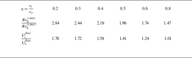


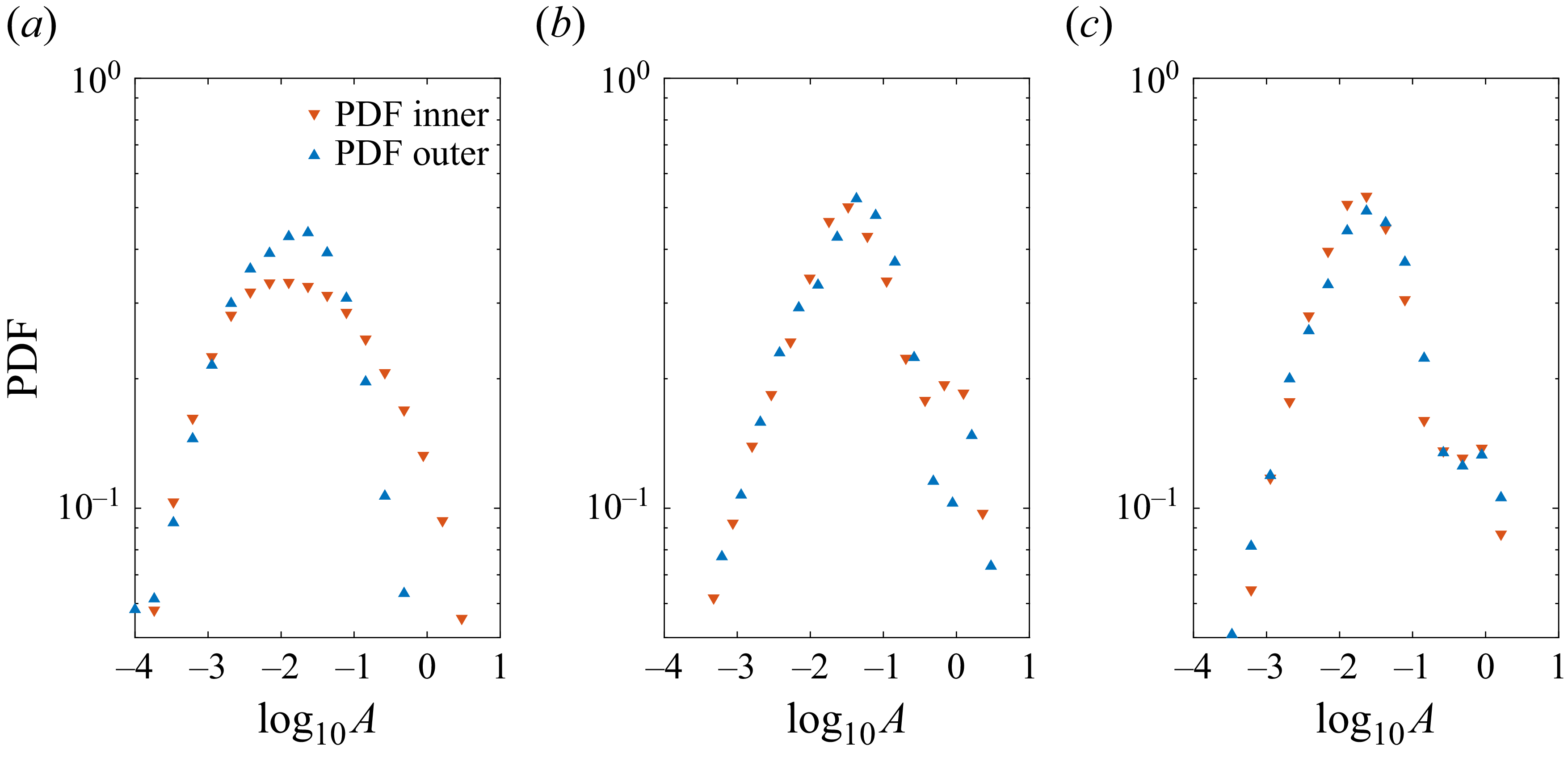


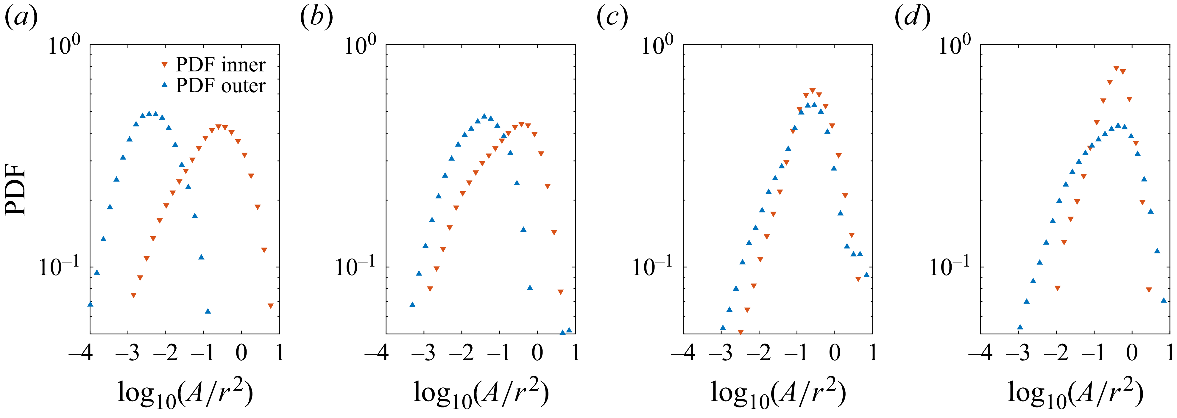


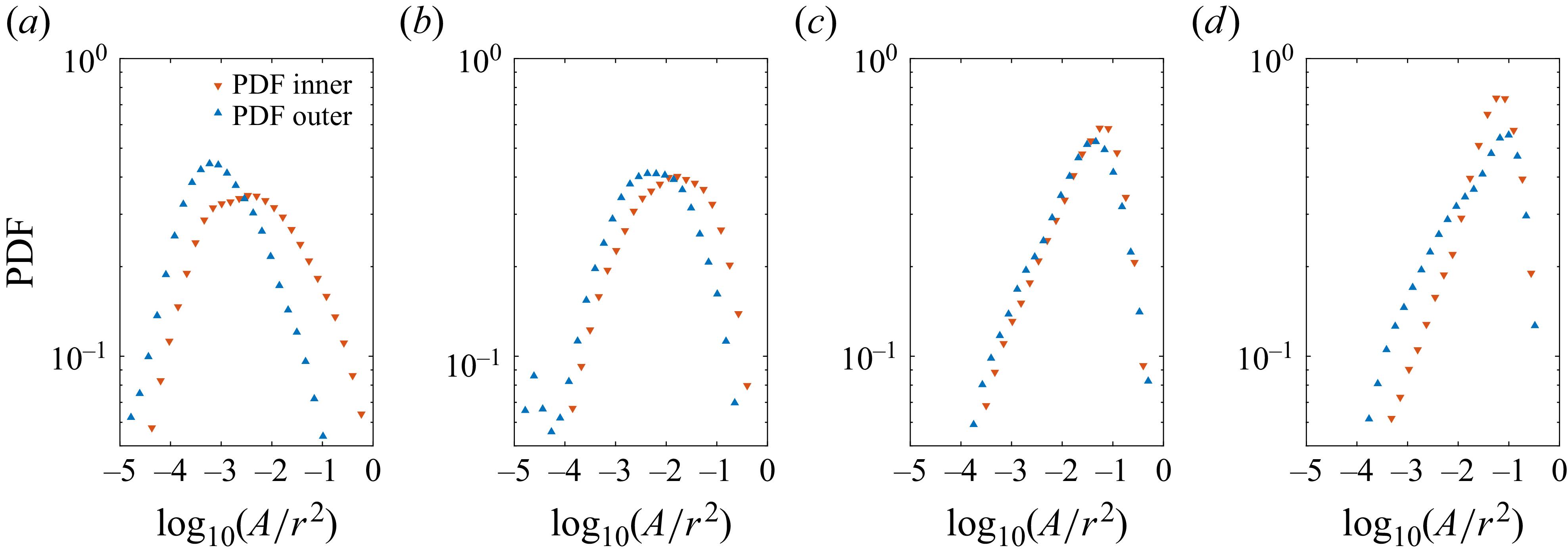


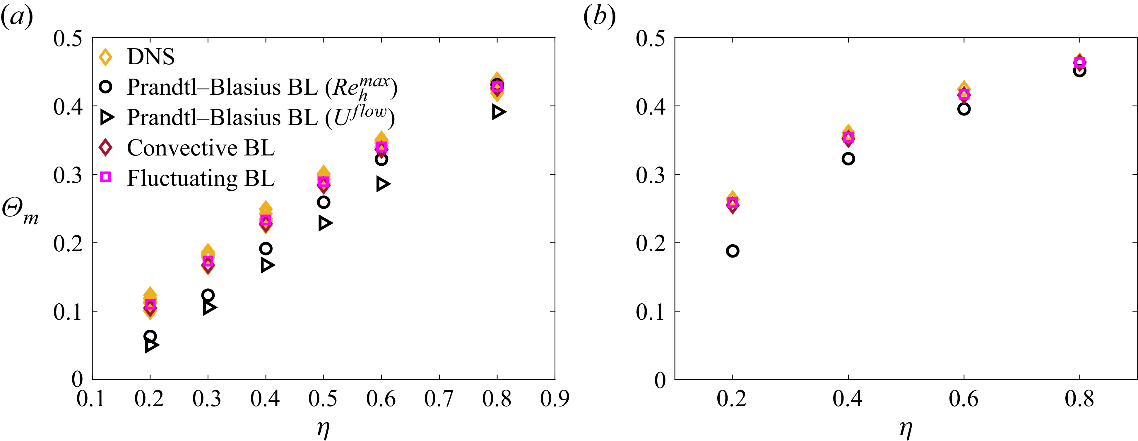


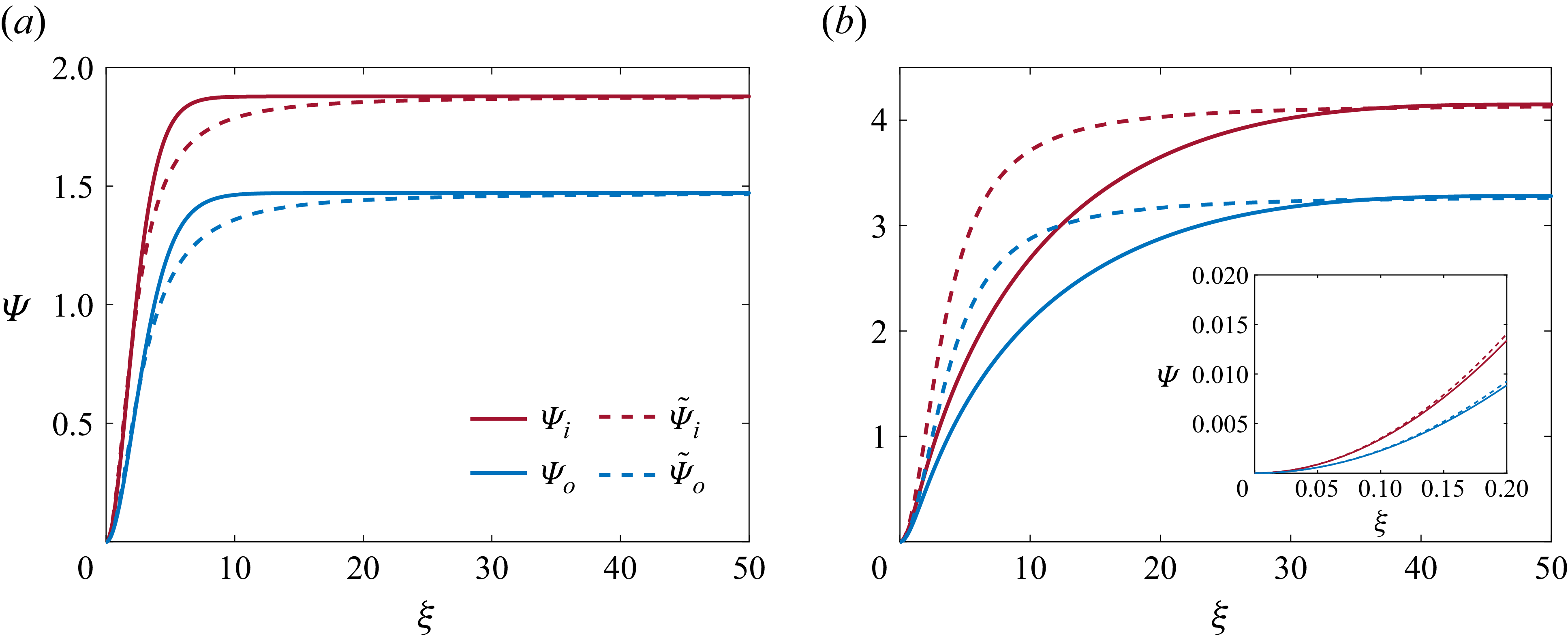


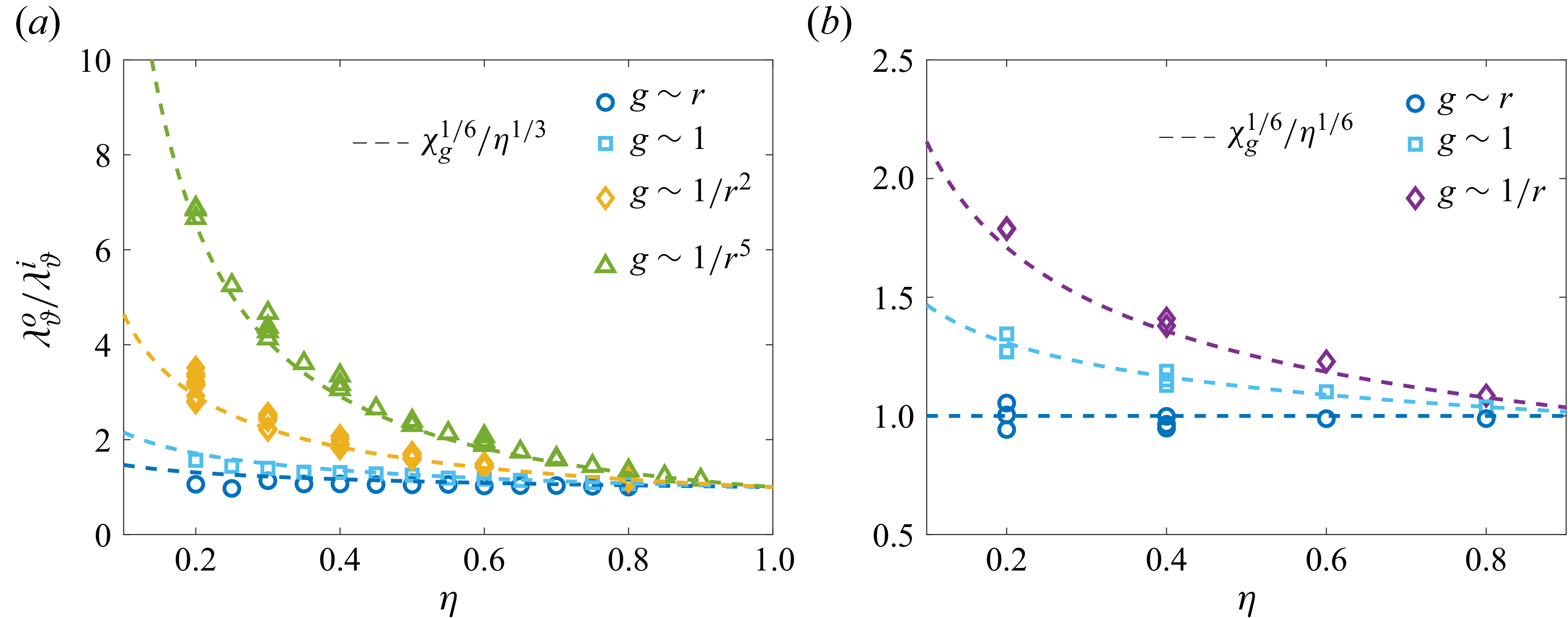


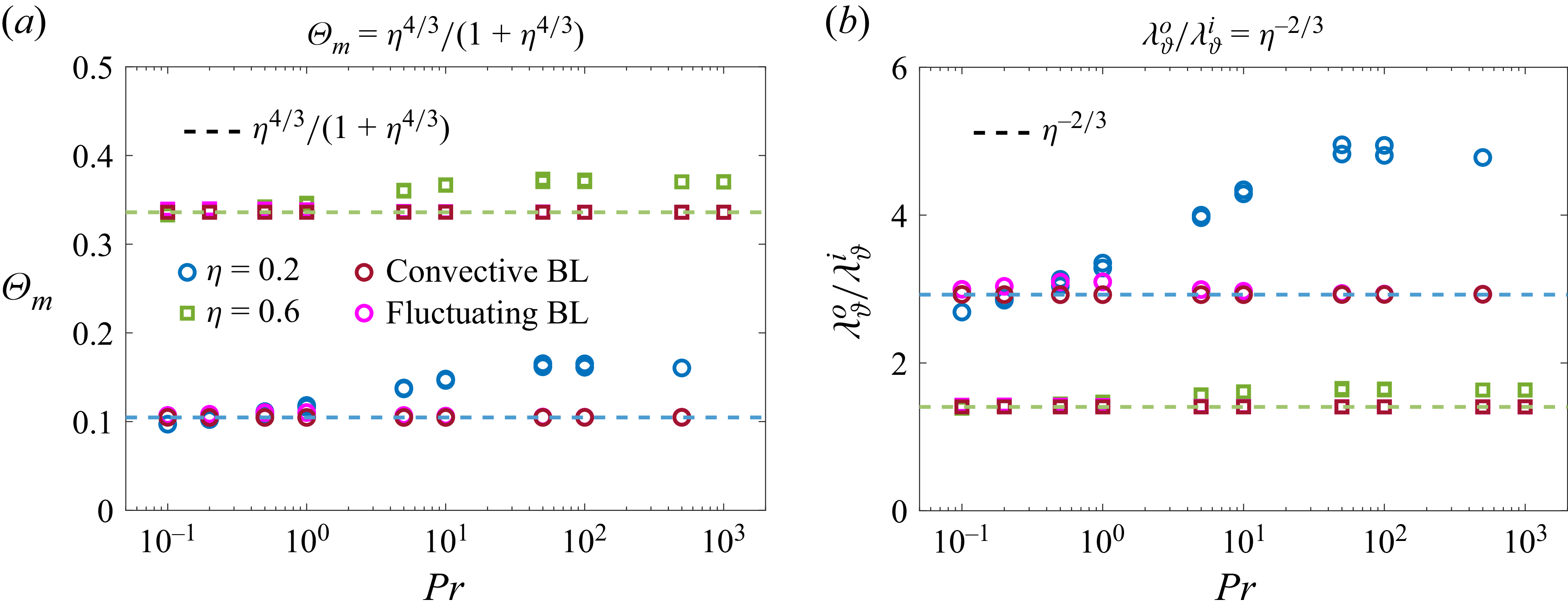


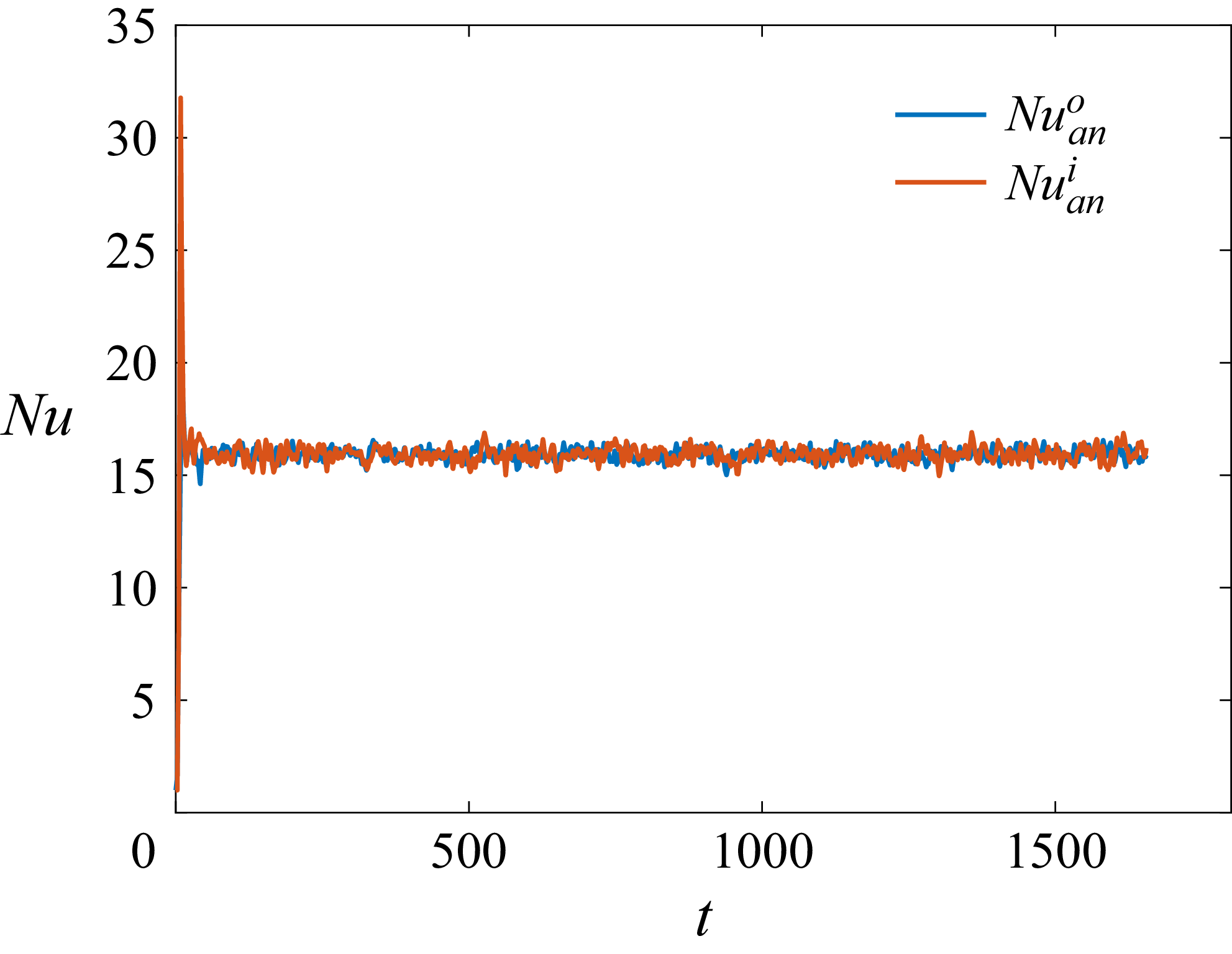


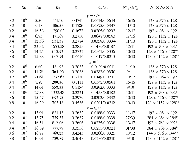


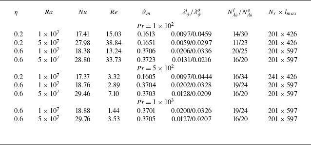


 Open access